Regional Characteristics of Unit Hydrographs and Storm

HyetographsTheodore G. Cleveland, Ph.D., P.E.

Instantaneous Unit Hydrograph Approach

• Unit hydrograph is one of several methods examined in this research.

• University of Houston has focused exclusively on this technique.

• Two major components– Analysis (Find IUH from rainfall-runoff data)– Synthesis (Estimate IUH from watershed

character)

Storm Analysis

• Central Texas Database• Analyze all storms using five different IUH model

equations.• Pick a “good” model• Aggregate model parameter values by station.• Re-run each storm using the aggregated values.• Test these results for acceptability• Interpret results• Conclusions and Recommendations

Central Texas Database

Different Unit Hydrograph Models

• Five IUH Models– Gamma– Rayleigh– Weibull – NRCS (DUH as an IUH)– Commons

Gamma-family

• Gamma, Rayleigh, and Weibull are all generalized gamma-distributions. The IUH model equation is

• Gamma when p=1; Rayleigh when p=2

)exp()( 1 p

pNp

pNp

p

p

t

t

t

t

t

tp

A

tq

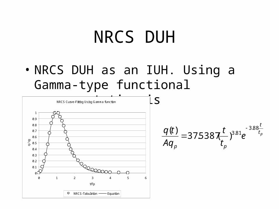
NRCS DUH

• NRCS DUH as an IUH. Using a Gamma-type functional representation is

pt

t

pp

et

t

Aq

tq 88.381.3)(5387.37

)(

NRCS Curve-Fitting Using Gamma function

0

0.1

0.2

0.3

0.4

0.5

0.6

0.7

0.8

0.9

1

0 1 2 3 4 5 6

t/Tp

q/qp

NRCS-Tabulation Equation

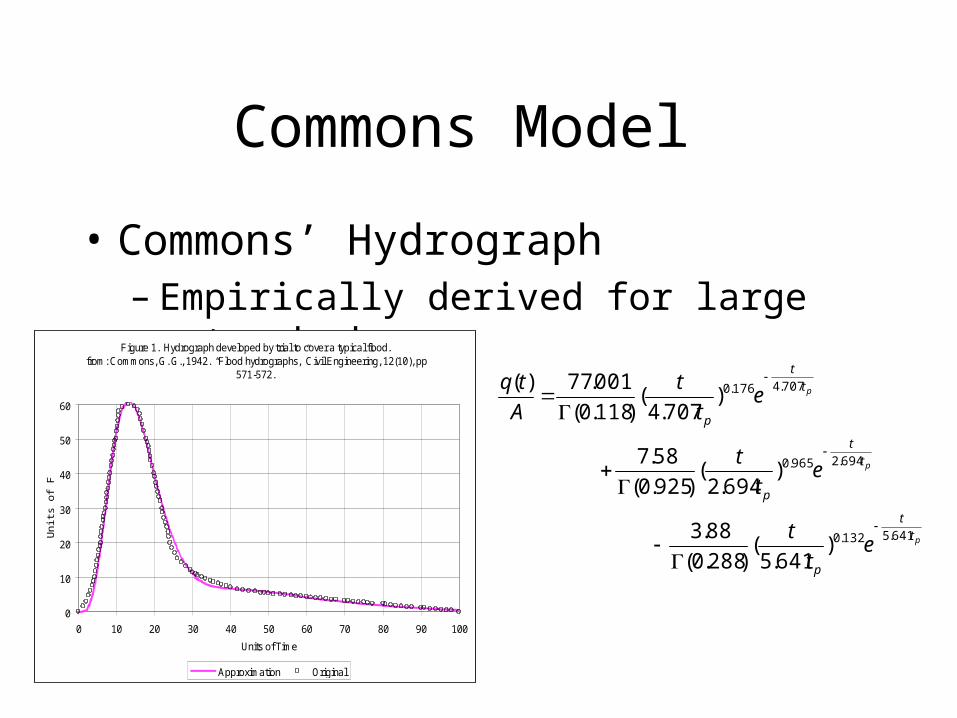
Commons Model

• Commons’ Hydrograph– Empirically derived for large watersheds

Figure 1. Hydrograph developed by trial to cover a typical flood. from: Commons, G. G., 1942. “Flood hydrographs,” Civil Engineering, 12(10), pp

571-572.

0

10

20

30

40

50

60

0 10 20 30 40 50 60 70 80 90 100

Units of Time

Uni

ts o

f Flo

w

Approximation Original

p

p

p

t

t

p

t

t

p

t

t

p

et

t

et

t

et

t

A

tq

641.5132.0

694.2965.0

707.4176.0

)641.5

()288.0(

88.3

)694.2

()925.0(

58.7

)707.4

()118.0(

001.77)(

Analyze Each Storm

• Supply observed precipitation data to the hydrograph function.

• Convolution of sequence of the IUH models to create a DRH.

• Compare observed runoff with DRH, adjust parameters in IUH to minimize some error function.

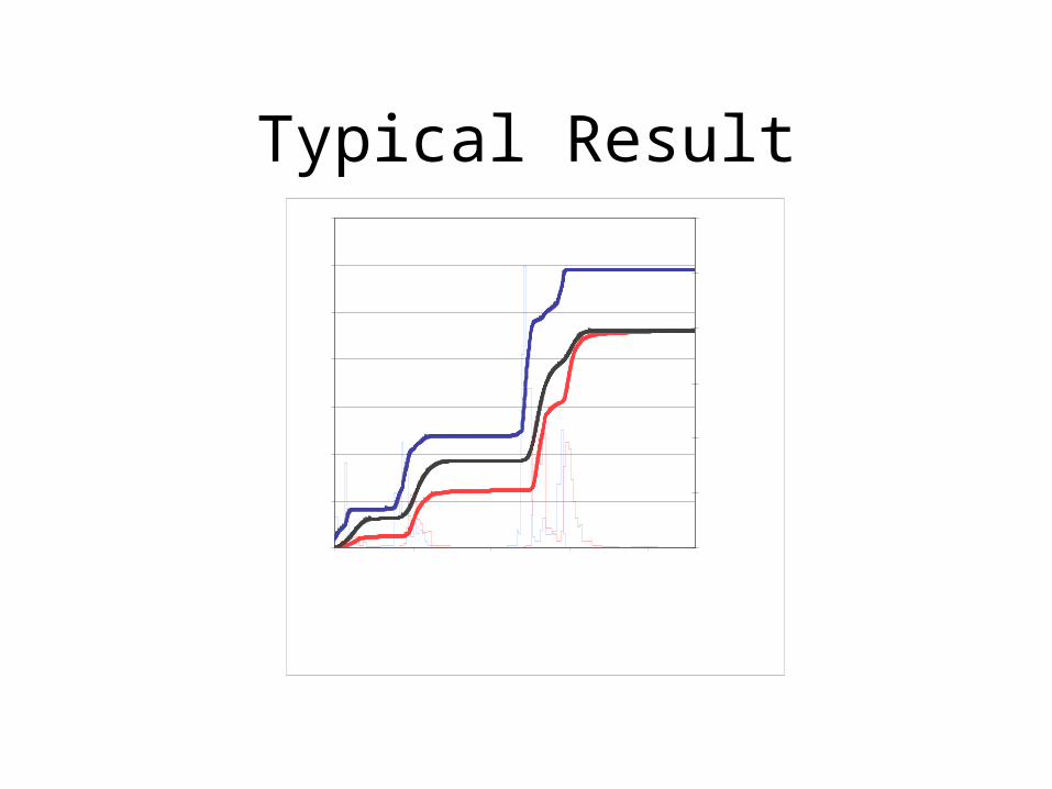
Typical Result

0

1

2

3

4

5

6

7

100 600 1100 1600 2100

Time (minutes)

Cu

mu

lati

ve D

epth

(in

ches

)

0.00E+00

1.00E-02

2.00E-02

3.00E-02

4.00E-02

5.00E-02

6.00E-02

Rat

e (i

nch

es/m

in)

ACC_PRECIP(IN) ACC_RUNOFF(IN)

ACC_MOD_RUNOFF(IN/MIN) RATE_PRECIP(IN/MIN)

RATE_RUNOFF(IN/MIN) RATE_MODEL(IN/MIN)

Figure 7.4 Plot of Observed and Model Runoff, Ash Creek, June 3, 1973 storm using the Weibull IUH model.

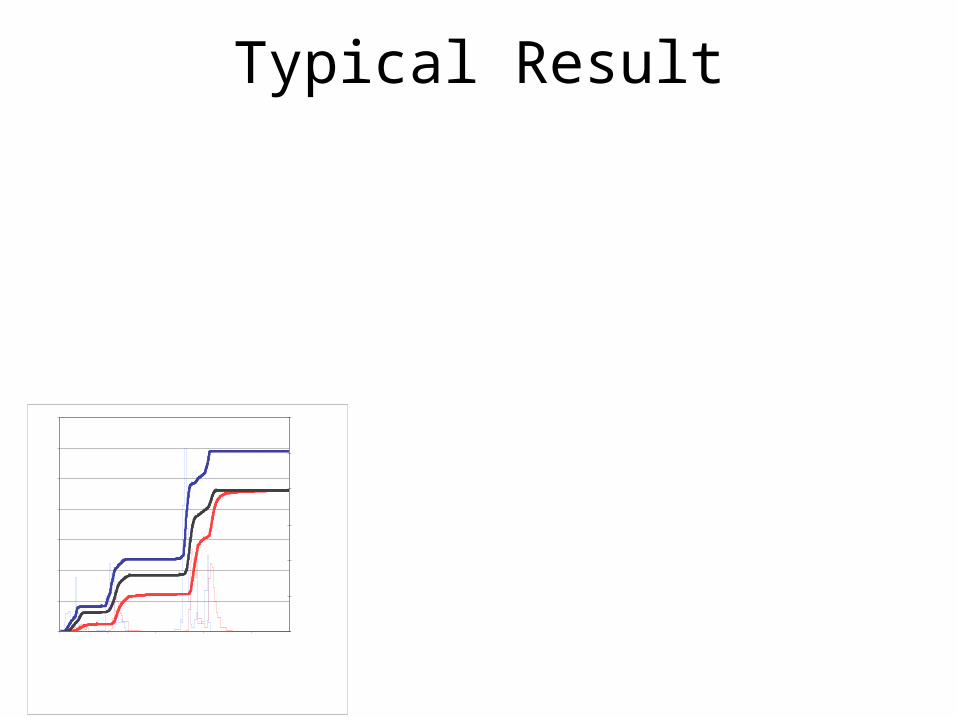
Typical Result

0

1

2

3

4

5

6

7

0 500 1000 1500 2000

Time (minutes)

Cu

mu

lati

ve D

epth

(in

ches

)

0.00E+00

1.00E-02

2.00E-02

3.00E-02

4.00E-02

5.00E-02

6.00E-02

Rat

e (i

nch

es/m

in)

ACC_PRECIP(IN) ACC_RUNOFF(IN)

ACC_MOD_RUNOFF(IN/MIN) RATE_PRECIP(IN/MIN)

RATE_RUNOFF(IN/MIN) RATE_MODEL(IN/MIN)

0

1

2

3

4

5

6

7

0 500 1000 1500 2000

Time (minutes)

Cu

mu

lati

ve D

epth

(in

ches

)

0.00E+00

1.00E-02

2.00E-02

3.00E-02

4.00E-02

5.00E-02

6.00E-02

Rat

e (i

nch

es/m

in)

ACC_PRECIP(IN) ACC_RUNOFF(IN)

ACC_MOD_RUNOFF(IN/MIN) RATE_PRECIP(IN/MIN)

RATE_RUNOFF(IN/MIN) RATE_MODEL(IN/MIN)

0

1

2

3

4

5

6

7

0 500 1000 1500 2000

Time (minutes)

Cu

mu

lati

ve D

epth

(in

ches

)

0.00E+00

1.00E-02

2.00E-02

3.00E-02

4.00E-02

5.00E-02

6.00E-02

Rat

e (i

nch

es/m

in)

ACC_PRECIP(IN) ACC_RUNOFF(IN)

ACC_MOD_RUNOFF(IN/MIN) RATE_PRECIP(IN/MIN)

RATE_RUNOFF(IN/MIN) RATE_MODEL(IN/MIN)

0

1

2

3

4

5

6

7

0 500 1000 1500 2000

Time (minutes)

Cu

mu

lati

ve D

epth

(in

ches

)

0.00E+00

1.00E-02

2.00E-02

3.00E-02

4.00E-02

5.00E-02

6.00E-02

Rat

e (i

nch

es/m

in)

ACC_PRECIP(IN) ACC_RUNOFF(IN)

ACC_MOD_RUNOFF(IN/MIN) RATE_PRECIP(IN/MIN)

RATE_RUNOFF(IN/MIN) RATE_MODEL(IN/MIN)

Commons

NRCS

Rayleigh

Gamma

Choosing a Model

• Establish acceptance criteria:– Averages

• Bias

• Fractional Bias

• Fractional Variance

• Normalized Mean Square Error

– Peak• Peak Relative Error:• Peak Temporal Bias:

PmPo ttTB

PoPmPo QQQQB /

N

iimiomo QQ

NQQBias

1,,

1

mo

mo

QQ

QQFB 2

qmqo

qmqoFV

22

22

2

mo

mo

QQ

QQNMSE

2

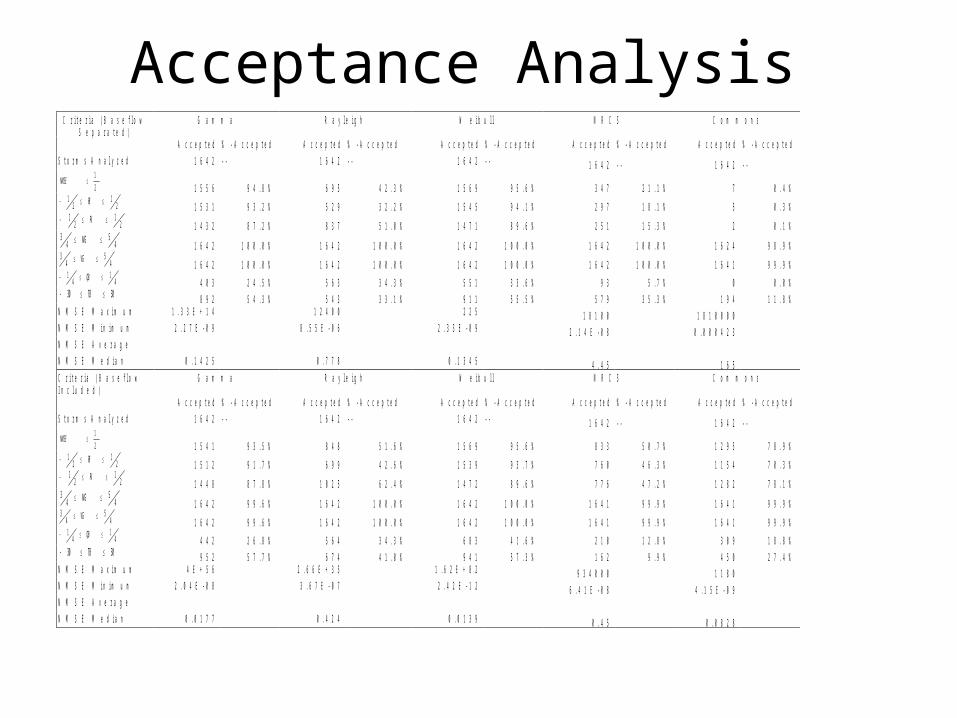
Acceptance AnalysisC r i t e r i a ( B a s e f l o w

S e p a r a t e d ) G a m m a R a y l e i g h W e i b u l l N R C S C o m m o n s

A c c e p t e d % - A c c e p t e d A c c e p t e d % - A c c e p t e d A c c e p t e d % - A c c e p t e d A c c e p t e d % - A c c e p t e d A c c e p t e d % - A c c e p t e d

S t o r m s A n a l y z e d 1 6 4 2 - - 1 6 4 2 - - 1 6 4 2 - - 1 6 4 2 - - 1 6 4 2 - -

2

1NMSE

1 5 5 6 9 4 . 8 % 6 9 5 4 2 . 3 % 1 5 6 9 9 5 . 6 % 3 4 7 2 1 . 1 % 7 0 . 4 %

21

21 FB

1 5 3 1 9 3 . 2 % 5 2 9 3 2 . 2 % 1 5 4 5 9 4 . 1 % 2 9 7 1 8 . 1 % 5 0 . 3 %

21

21 FV

1 4 3 2 8 7 . 2 % 8 3 7 5 1 . 0 % 1 4 7 1 8 9 . 6 % 2 5 1 1 5 . 3 % 2 0 . 1 %

45

43 MG

1 6 4 2 1 0 0 . 0 % 1 6 4 2 1 0 0 . 0 % 1 6 4 2 1 0 0 . 0 % 1 6 4 2 1 0 0 . 0 % 1 6 2 4 9 8 . 9 %

45

43 VG

1 6 4 2 1 0 0 . 0 % 1 6 4 2 1 0 0 . 0 % 1 6 4 2 1 0 0 . 0 % 1 6 4 2 1 0 0 . 0 % 1 6 4 1 9 9 . 9 %

41

41 QB

4 0 3 2 4 . 5 % 5 6 3 3 4 . 3 % 5 5 1 3 3 . 6 % 9 3 5 . 7 % 0 0 . 0 %

3030 TB 8 9 2 5 4 . 3 % 5 4 3 3 3 . 1 % 9 1 1 5 5 . 5 % 5 7 9 3 5 . 3 % 1 9 4 1 1 . 8 % N M S E M a x i m u m 1 . 3 3 E + 1 4 1 2 4 0 0 2 2 5 1 8 1 0 0 1 8 1 0 0 0 0 N M S E M i n i m u m 2 . 2 7 E - 0 9 8 . 5 5 E - 0 6 2 . 3 3 E - 0 9 2 . 1 4 E - 0 8 0 . 0 0 0 4 2 3 N M S E A v e r a g e N M S E M e d i a n 0 . 1 4 2 5 0 . 7 7 8 0 . 1 3 4 5 4 . 4 5 1 6 5 C r i t e r i a ( B a s e f l o w I n c l u d e d )

G a m m a R a y l e i g h W e i b u l l N R C S C o m m o n s

A c c e p t e d % - A c c e p t e d A c c e p t e d % - A c c e p t e d A c c e p t e d % - A c c e p t e d A c c e p t e d % - A c c e p t e d A c c e p t e d % - A c c e p t e d

S t o r m s A n a l y z e d 1 6 4 2 - - 1 6 4 2 - - 1 6 4 2 - - 1 6 4 2 - - 1 6 4 2 - -

2

1NMSE

1 5 4 1 9 3 . 5 % 8 4 8 5 1 . 6 % 1 5 6 9 9 5 . 6 % 8 3 3 5 0 . 7 % 1 2 9 5 7 8 . 9 %

21

21 FB

1 5 1 2 9 1 . 7 % 6 9 9 4 2 . 6 % 1 5 3 9 9 3 . 7 % 7 6 0 4 6 . 3 % 1 1 5 4 7 0 . 3 %

21

21 FV

1 4 4 8 8 7 . 8 % 1 0 2 5 6 2 . 4 % 1 4 7 2 8 9 . 6 % 7 7 6 4 7 . 2 % 1 2 8 2 7 8 . 1 %

45

43 MG

1 6 4 2 9 9 . 6 % 1 6 4 2 1 0 0 . 0 % 1 6 4 2 1 0 0 . 0 % 1 6 4 1 9 9 . 9 % 1 6 4 1 9 9 . 9 %

45

43 VG

1 6 4 2 9 9 . 6 % 1 6 4 2 1 0 0 . 0 % 1 6 4 2 1 0 0 . 0 % 1 6 4 1 9 9 . 9 % 1 6 4 1 9 9 . 9 %

41

41 QB

4 4 2 2 6 . 8 % 5 6 4 3 4 . 3 % 6 8 3 4 1 . 6 % 2 1 0 1 2 . 8 % 3 0 9 1 8 . 8 %

3030 TB 9 5 2 5 7 . 7 % 6 7 4 4 1 . 0 % 9 4 1 5 7 . 3 % 1 6 2 9 . 9 % 4 5 0 2 7 . 4 % N M S E M a x i m u m 4 E + 5 6 2 . 6 6 E + 3 5 1 . 6 2 E + 8 2 9 3 4 0 0 0 1 1 8 0 N M S E M i n i m u m 2 . 0 4 E - 0 8 3 . 6 7 E - 0 7 2 . 4 2 E - 1 2 6 . 4 1 E - 0 8 4 . 1 5 E - 0 9 N M S E A v e r a g e N M S E M e d i a n 0 . 0 1 7 7 0 . 4 2 4 0 . 0 1 3 9 0 . 4 5 0 . 0 8 2 8

Acceptance Analysis

• Aggregate model parameter values by station.– Test if parameter values depend on station or are

independent. (Dependent)

• Re-run each storm using the aggregated values.– (In-Progress)

• Test these results for acceptability– (Pending)

Interim Conclusions

• Parameter values vary by station and module. (Jonnalagadda, 2003)

• Weibull model is reasonable IUH model (He, 2004).References: Xin, He. 2004. Comparison of Gamma, Rayleigh, Weibull and NRCS Models with Observed Runoff Data for Central Texas Small Watersheds. Master's Thesis. Department of Civil and Environmental Engineering, University of Houston, Houston, Texas. 90p.Jonalagadda, Krishna, 2003. Determination of Instantaneous Unit Hydrographs for Small Watersheds of Central Texas. Master's Thesis. Department of Civil and Environmental Engineering, University of Houston, Houston, Texas. 132p.

Synthesis

• Evaluate methods to synthesize hydrographs in absence of data.

• Fundamental assumption: Watershed characteristics (slope, length, etc.) are predictors of hydrologic response and thus are predictors of IUH parameter values, and that there exists a UH.

Synthesis

• Determine watershed characteristics– Area, perimeter, slopes, lengths, etc.

• Relate regression models to IUH parameters to selected watershed characteristics.

• Use regression model to determine parameter values by station.

• Run each storm using these values.• Test results for acceptability• Interpret results• Make Conclusions and Recommendations

Watershed Characteristics

• These are measurements that can be made from a map, air photo, or possibly field visit.– Area, slope, etc.– Manual determination (University of Houston,

checked and corrected by Lamar)– Automated determination (USGS)

Regression Models• Power Law Model (representative)

• Weights determined by minimization of RMS error between “observed” IUH parameters and the power law model.

• Predict values of IUH model (t_bar,p,N) from watershed characteristics, then use resulting IUH.

SlopeStreamx

ShapeRatiox

PerimeterAreax

SlopeRawx

RatioAspectx

Areax

resNy

py

barty

xxxxxxwy wi

wi

wi

wi

wi

wioi

_

/

_

_

_

_

6

5

4

3

2

1

3

2

1

,6,5,4,3,2,1654321

Typical Interim Results

Tp(hrs) versus SQRT(Area)All Watersheds

0.1

1

10

100

0.1 1 10 100

SQRT(Area (mi 2))

Tim

e (h

rs)

Tp = 0.64*SQRT(Area)

Interim Conclusions

• Analysis of selected small, medium, and large watersheds in each module was used to test feasibility of approach

– The power-law model can produce parameter values that, when used as the IUH model could match peak discharge rates to within 15% of observed values, and match the arrival time of the peak within an hour.

References

Lazarescu, Ioana, 2003. Correlation of Geometric Properties of Small Watersheds in Central Texas with Observed Instantaneous Unit Hydrographs Master's Thesis. Department of Civil and Environmental Engineering, University of Houston, Houston, Texas. 84p.

Remaining Work

• Storm analysis– Aggregate results, perform comparisons and

acceptance tests. (in-progress)– Interpret results in raw form and transform into

conventional Qp,Tp,Tc format. (pending above)– Write research report. (in-progress)

Remaining Work

• Regionalization– Power-law model of entire data set (not just subset used

in Lazarescu’s thesis).– Interpret results, select most meaningful watershed

characteristic combinations. – Test with all storms, apply acceptance criteria.– Compare with NRCS methods to synthesize Unitgraphs

• 90 TR-20 models to be created this summer.

– Write research report with methodology and guidelines for use (Report started, quite empty).