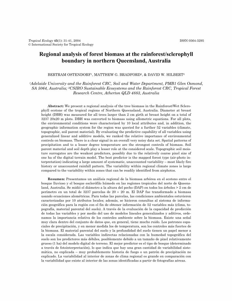
OSTENDORF, BRADFORD & HILBERT 31

Tropical Ecology 45(1): 31-41, 2004 ISSN 0564-3295 © International Society for Tropical Ecology

Regional analysis of forest biomass at the rainforest/sclerophyll boundary in northern Queensland, Australia

BERTRAM OSTENDORF1, MATTHEW G. BRADFORD2, & DAVID W. HILBERT2

1Adelaide University and the Rainforest CRC, Soil and Water Department, PMB1 Glen Osmond, SA 5064, Australia; 2CSIRO Sustainable Ecosystems and the Rainforest CRC, Tropical Forest

Research Centre, Atherton QLD 4883, Australia

Abstract: We present a regional analysis of the tree biomass in the Rainforest/Wet Sclero-phyll ecotone of the tropical regions of Northern Queensland, Australia. Diameter at breast height (DBH) was measured for all trees larger than 2 cm girth at breast height on a total of 3237 20x20 m plots. DBH was converted to biomass using allometric equations. For all plots, the environmental conditions were characterized by 10 local attributes and, in addition, the geographic information system for the region was queried for a further 52 variables (climate, topographic, soil parent material). By evaluating the predictive capability of all variables using generalized linear and additive models, we ranked the relative importance of environmental controls on biomass. There is a clear signal in an overall very noisy data set. Spatial patterns of precipitation and to a lesser degree temperature are the strongest controls of biomass. Soil parent material and soil depth play a lesser role at the considered scale. Topographic soil mois-ture surrogates are the weakest predictors, possibly due to the relatively coarse pixel size of one ha of the digital terrain model. The best predictor is the mapped forest type (air-photo in-terpretation) indicating a large amount of systematic, unaccounted variability – most likely fire history or unaccounted rainfall pattern. The variability within regional climate zones is large compared to the variability within zones that can be readily identified from airphotos.

Resumen: Presentamos un análisis regional de la biomasa arbórea en el ecotono entre el

bosque lluvioso y el bosque esclerófilo húmedo en las regiones tropicales del norte de Queens-land, Australia. Se midió el diámetro a la altura del pecho (DAP) en todos los árboles > 2 cm de perímetro en un total de 3237 parcelas de 20 × 20 m. El DAP fue transformado a biomasa usando ecuaciones alométricas. Para todas las parcelas, las condiciones ambientales estuvieron caracterizadas por 10 atributos locales; además, se hicieron consultas al sistema de informa-ción geográfica para la región con el fin de obtener información de 52 variables más (clima, to-pografía, material parental del suelo). A través de la evaluación de la capacidad de predicción de todas las variables y por medio del uso de modelos lineales generalizados y aditivos, orde-namos la importancia relativa de los controles ambiente sobre la biomasa. Existe una señal muy clara dentro del conjunto de datos que, en general, tiene mucho ruido. Los patrones espa-ciales de precipitación, y en menor medida los de temperatura, son los controles más fuertes de la biomasa. El material parental del suelo y la profundidad del suelo tienen un papel menor a la escala considerada. Las variables indirectas relacionadas con la humedad topográfica del suelo son los predictores más débiles, posiblemente debido a un tamaño de pixel relativamente grueso (1 ha) del modelo digital de terreno. El mejor predictor es el tipo de bosque (determinado a través de fotointerpretación), lo que indica que hay una gran cantidad de variabilidad siste-mática, no explicada – muy probablemente historia de fuego o un patrón de precipitación no explicado. La variabilidad al interior de zonas de clima regional es grande en comparación con la variabilidad que existe al interior de las zonas identificadas a partir de fotografías aéreas.

32 FOREST BIOMASS IN QUEENSLAND

Resumo: Apresenta-se uma análise regional da biomassa arbórea no ecotono Floresta de Chuvas / Esclerófita Húmida nas regiões tropicais do Norte de Queensland, Austrália. O diâmetro à altura do peito (DAP) foi medido para todas as árvores com diâmetro à altura do peito superior a 2 cm num total de 3237 em parcelas de 20*20 m. O DAP foi convertido em biomassa usando equações alométricas. Para todas as parcelas as condições ambientais foram caracterizadas com recurso a 10 atributos locais e, adicionalmente, o sistema de informação geográfica para a região foi consultado para extracção de mais de 52 variáveis (clima, to-pografia, rocha mãe do solo). Pela avaliação da capacidade preditiva de todas as variáveis, com recurso a modelos lineares e aditivos, ordenámos a importância relativa dos controles ambien-tais sobre a biomassa. Há sinais claros de uma forte dispersão dos dados. O padrão espacial da precipitação e em menor grau a temperatura são os principais parâmetros que controlam a biomassa. A rocha mãe do solo e a sua profundidade jogam um papel menor na escala consid-erada. A topografia e a correspondente humidade do solo foram os preditores mais fracos, pos-sivelmente devido ao grão elevado dos pixel do modelo de representação digital de um ha de terreno utilizado. O melhor preditor é o tipo florestal mapeado (foto-interpretada), indicando uma quantidade elevada e sistemática, de variabilidade não considerada – muito provavel-mente a história dos fogos ou padrões de precipitação. A variabilidade dentro das zonas climáticas regionais é fortemente comparável à variabilidade dentro das zonas que podem ser prontamente identificadas a partir das fotografias aéreas.

Key words: Australia, biomass, climate change, general linear model, generalized additive model, spa-

tial variability, tall open forests, topographic analysis, wet sclerophyll (Eucalypt and Aca-cia species), wet tropics.

Introduction

Understanding the carbon storage of the bio-sphere is important for its role in the global carbon cycle, and the need to predict biomass and primary productivity patterns has not lost its urgency since the pioneering work of Lieth (1972). Studies of re-gional vegetation patterns reveal that vegetation types may be sensitive to temperature changes as little as one degree (Box et al. 1999; Hilbert et al. 2001; Hilbert & Ostendorf 2001; Iverson et al. 1999). Our ability to measure carbon exchange rates with the atmosphere has been substantially improved, but what actually determines the spa-tial pattern of biomass is still not understood.

Tropical regions are receiving increased atten-tion due to their importance in the global carbon cycle (Justice et al. 2001; Nascimento & Laurance 2002). Assessment of the future state of the bio-sphere, including biomass, productivity and biodi-versity, however, ultimately relies on field data, and these are difficult to collect because of spatial and temporal variability (e.g. Ostendorf et al. 2001a). This is particularly evident for tropical

systems where remoteness and climate-related logistical difficulties add to the problem. A low number of objectively selected field locations often prohibits a regional analysis of environmental gradients. Brown & Lugo (1984) illustrated the difficulties in obtaining statistically sound biomass data and concluded that earlier estimates of the carbon content of tropical vegetation based on de-structive sampling were biased toward more pro-ductive plots. Understanding the causes of observ-able patterns will improve spatial sampling de-signs for future field studies and indicate the rela-tive importance of spatial surrogates, which may be used to interpolate and possibly extrapolate field data.

The tropical region of Northern Queensland, Australia provides a unique natural laboratory for several reasons. It exhibits steep climatic gradi-ents with annual precipitation of up to 8000 mm, gradients of more than 40 mm per km, and mean annual temperature ranges from 16 to 25°C. A large variety of different tropical and subtropical forest types (see Webb et al. 1959, 1968) occurs in close proximity. Furthermore, the Gondwanan ori-

OSTENDORF, BRADFORD & HILBERT 33

gin and richness of endemic species and the re-gion’s past economic potential for wood production and agriculture provide for a long history of eco-logical research at a regional scale.

The boundary between rainforest and wood-lands (sclerophyll forest types1) has been of par-ticular interest for land managers and ecologists in various tropical and subtropical regions. In Aus-tralia, this region provides habitat for several rare and endangered mammal and bird species (Winter et al. 1984). Since this boundary constitutes an ecotone, climate change may affect this vegetation belt most strongly (Hilbert et al. 2001; Hilbert & Ostendorf 2001). Ostendorf et al. (2001b) assessed the sensitivity of the model predictions to changes in model structure (including different spatial and ecological constraints on vegetation change) and found that vegetation types at the rainforest boundary are least predictable. Regional manage-ment and ecosystem conservation is challenging because of substantial knowledge gaps of the for-ests sensitivity to climate change, especially if one considers a possible increase of mean annual tem-perature by 2-4°C during the next 50 years (Walsh et al. 2000).

A comprehensive survey of forest structure was undertaken (Harrington et al. 2000) in the “Wet Tropics” region of Northern Queensland be-tween roughly –15 and –20° latitude. Basal area was recorded for all trees with a DBH >= 2 cm on a total of 3237 20x20 m plots at the rainforest boundary. A comprehensive set of site attributes was collected at each plot. Furthermore, vegetation was mapped using air photos and a regional classi-fication of different sclerophyll forest types. The small plot size was a compromise to obtain region-ally representative tree population information. In parallel, a comprehensive GIS was developed in-cluding a detailed digital terrain model (DTM), surfaces of climate and topographic variables and soil parent material.

In this paper we present a regional analysis of biomass in the rainforest/sclerophyll ecotone. We have conducted a statistical analysis of biomass and environmental conditions as represented by a set of 52 maps of environmental conditions and local plot descriptions. This allows a ranking of relative predictive capability of forest biomass for a comprehensive set of environmental variables.

Materials and methods

Study site The study region is the western edge of the

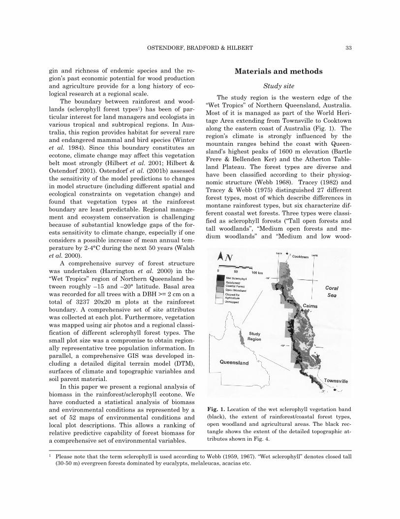
“Wet Tropics” of Northern Queensland, Australia. Most of it is managed as part of the World Heri-tage Area extending from Townsville to Cooktown along the eastern coast of Australia (Fig. 1). The region’s climate is strongly influenced by the mountain ranges behind the coast with Queen-sland’s highest peaks of 1600 m elevation (Bartle Frere & Bellenden Ker) and the Atherton Table-land Plateau. The forest types are diverse and have been classified according to their physiog-nomic structure (Webb 1968). Tracey (1982) and Tracey & Webb (1975) distinguished 27 different forest types, most of which describe differences in montane rainforest types, but six characterize dif-ferent coastal wet forests. Three types were classi-fied as sclerophyll forests (“Tall open forests and tall woodlands”, “Medium open forests and me-dium woodlands” and “Medium and low wood-

1 Please note that the term sclerophyll is used according to Webb (1959, 1967). “Wet sclerophyll” denotes closed tall (30-50 m) evergreen forests dominated by eucalypts, melaleucas, acacias etc.

Fig. 1. Location of the wet sclerophyll vegetation band(black), the extent of rainforest/coastal forest types,open woodland and agricultural areas. The black rec-tangle shows the extent of the detailed topographic at-tributes shown in Fig. 4.

34 FOREST BIOMASS IN QUEENSLAND

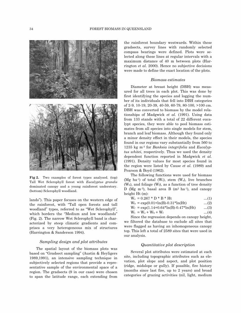
lands”). This paper focuses on the western edge of the rainforest, with “Tall open forests and tall woodland” types, referred to as “Wet Sclerophyll”, which borders the “Medium and low woodlands” (Fig. 2). The narrow Wet Sclerophyll band is char-acterized by steep climatic gradients and com-prises a very heterogeneous mix of structures (Harrington & Sanderson 1994).

Sampling design and plot attributes The spatial layout of the biomass plots was

based on “Gradsect sampling” (Austin & Heyligers 1989,1991), an intensive sampling technique in subjectively selected regions that provide a repre-sentative sample of the environmental space of a region. The gradsects (9 in our case) were chosen to span the latitude range, each extending from

the rainforest boundary westwards. Within these gradsects, survey lines with randomly selected compass bearings were defined. Plots were se-lected along these lines at regular intervals with a maximum distance of 40 m between plots (Har-rington et al. 2000). Hence no subjective decisions were made to define the exact location of the plots.

Biomass estimates Diameter at breast height (DBH) was meas-

ured for all trees in each plot. This was done by first identifying the species and logging the num-ber of its individuals that fell into DBH categories of 2-9, 10-19, 20-39, 40-59, 60-79, 80-100, >100 cm. DBH was converted to biomass by the model rela-tionships of Madgwick et al. (1991). Using data from 133 stands with a total of 22 different euca-lypt species, they were able to pool biomass esti-mates from all species into single models for stem, branch and leaf biomass. Although they found only a minor density effect in their models, the species found in our regions vary substantially from 560 to 1235 kg m-3 for Banksia integrifolia and Eucalyp-tus whitei, respectively. Thus we used the density dependent function reported in Madgwick et al. (1991). Density values for most species found in the region were listed by Cause et al. (1989) and Pearson & Boyd (1962).

The following functions were used for biomass (Mg ha-1) of total (Wt), stem (Ws), live branches (Wb), and foliage (Wf), as a function of tree density D (Mg m-3), basal area B (m2 ha-1), and canopy height Ht (m):

Ws = 0.267 * D * B * Ht …(1) Wb = exp(0.01+ln(B)-0.31*ln(Ht) …(2) Wf = exp(1.14+0.64*ln(B)-0.47*ln(Ht) …(3) Wt = Ws + Wb + Wf …(4) Since the regression depends on canopy height,

we filtered the database to exclude all sites that were flagged as having an inhomogeneous canopy top. This left a total of 2589 sites that were used in our analysis.

Quantitative plot description Several plot attributes were estimated at each

site, including topographic attributes such as ele-vation, plot slope and aspect, and plot position (ridge, midslope or gully). If possible, fire history (months since last fire, up to 2 years) and broad categories of grazing activities (nil, light, medium

Fig 2. Two examples of forest types analysed. (top)Tall Wet Sclerophyll forest with Eucalyptus grandisdominated canopy and a young rainforest understory.(bottom) Sclerophyll woodland.

OSTENDORF, BRADFORD & HILBERT 35

or heavy) were noted. Soil depth was recorded as “shallow” (<5 cm), “average” (5-100 cm) or “deep” (>100 cm), and soil parent-material classes were distinguished (granite, rhyollite, basalt, metamor-phic, alluvium). For more detail see Harrington et al. (2000).

Spatial data The spatial data layers in the geographic in-

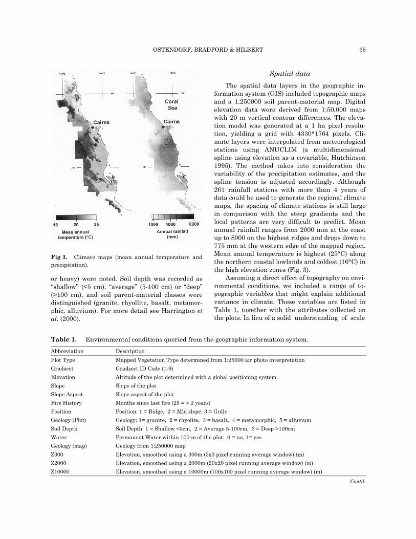
formation system (GIS) included topographic maps and a 1:250000 soil parent-material map. Digital elevation data were derived from 1:50,000 maps with 20 m vertical contour differences. The eleva-tion model was generated at a 1 ha pixel resolu-tion, yielding a grid with 4330*1764 pixels. Cli-mate layers were interpolated from meteorological stations using ANUCLIM (a multidimensional spline using elevation as a covariable, Hutchinson 1995). The method takes into consideration the variability of the precipitation estimates, and the spline tension is adjusted accordingly. Although 261 rainfall stations with more than 4 years of data could be used to generate the regional climate maps, the spacing of climate stations is still large in comparison with the steep gradients and the local patterns are very difficult to predict. Mean annual rainfall ranges from 2000 mm at the coast up to 8000 on the highest ridges and drops down to 775 mm at the western edge of the mapped region. Mean annual temperature is highest (25°C) along the northern coastal lowlands and coldest (16°C) in the high elevation zones (Fig. 3).

Assuming a direct effect of topography on envi-ronmental conditions, we included a range of to-pographic variables that might explain additional variance in climate. These variables are listed in Table 1, together with the attributes collected on the plots. In lieu of a solid understanding of scale

Fig 3. Climate maps (mean annual temperature andprecipitation).

Table 1. Environmental conditions queried from the geographic information system. Abbreviation Description Plot Type Mapped Vegetation Type determined from 1:25000 air photo interpretation Gradsect Gradsect ID Code (1-9) Elevation Altitude of the plot determined with a global positioning system Slope Slope of the plot Slope Aspect Slope aspect of the plot Fire History Months since last fire (25 = > 2 years) Position Position: 1 = Ridge, 2 = Mid slope, 3 = Gully Geology (Plot) Geology: 1= granite, 2 = rhyolite, 3 = basalt, 4 = metamorphic, 5 = alluvium Soil Depth Soil Depth: 1 = Shallow <5cm, 2 = Average 5-100cm, 3 = Deep >100cm Water Permanent Water within 100 m of the plot: 0 = no, 1= yes Geology (map) Geology from 1:250000 map Z300 Elevation, smoothed using a 300m (3x3 pixel running average window) (m) Z2000 Elevation, smoothed using a 2000m (20x20 pixel running average window) (m) Z10000 Elevation, smoothed using a 10000m (100x100 pixel running average window) (m)

Contd.

36 FOREST BIOMASS IN QUEENSLAND

Table 1 Contd.. Abbreviation Description T (mean) Annual Mean Temperature (°C) T (wet) Mean Temperature of Wettest Quarter (°C) T (dry) Mean Temperature of Driest Quarter (°C) T (warm) Mean Temperature of Warmest Quarter (°C) T (cold) Mean Temperature of Coldest Quarter (°C) P (mean) Annual Precipitation (mm) P (wet) Precipitation of Wettest Quarter (mm) P (dry) Precipitation of Driest Quarter (mm) P (warm) Precipitation of Warmest Quarter (mm) P (cold) Precipitation of Coldest Quarter (mm) Dist coast Distance to coast (m) Dist drainage Distance to drainage lines(m) Dist per Distance to perennial streams (m) cur 300 N Curvature in North/South direction using Z300 (0°); all slope estimates are dimensionless, curva-

ture estimates are in m-1 cur 2000 N Curvature in North/South direction using Z2000 (0°) cur 10000 N Curvature in North/South direction using Z10000 (0°) cur 300 NE Curvature in North-East/South-West direction using Z300 (45°) cur 2000 NE Curvature in North-East/South-West direction using Z2000 (45°) cur 10000 NE Curvature in North-East/South-West direction using Z10000 (45°) cur 300 W Curvature East/West (90°) using Z300 cur 2000 W Curvature East/West (90°) using Z2000 cur 10000 W Curvature East/West (90°) using Z10000 cur 300 SE Curvature in South-East/North-West direction (135°) using Z300 cur 2000 SE Curvature in South-East/North-West direction (135°) using Z2000 cur 10000 SE Curvature in South-East/North-West direction (135°) using Z10000 slp 300 N Slope towards North using Z300 slp 2000N Slope towards North using Z2000 slp 10000 N Slope towards North using Z10000 slp 300 NE Slope towards Northeast using Z300 slp 2000 NE Slope towards Northeast using Z2000 slp 10000 NE Slope towards Northeast using Z10000 slp 300 W Slope towards East using Z300 slp 2000 W Slope towards East using Z2000 slp 10000 W Slope towards East using Z10000 slp 300 SE Slope towards Southeast using Z300 slp 2000 SE Slope towards Southeast using Z2000 slp 10000 SE Slope towards Southeast using Z10000 drain.0 Drainage area; contributing area per contour length (m) drain 300 Drainage area (m) using Z300 (m) drain 2000 Drainage area (m) using Z2000 (m) drain 10000 Drainage area (m) using Z10000 (m) drain p Average annual discharge; volume rainfall per contour length (m2 yr-1) drain p 300 Average annual discharge using Z300 (m2 yr-1) drain p 2000 Average annual discharge using Z2000 (m2 yr-1) drain p 10000 Average annual discharge using Z10000 (m2 yr-1) Pot. solar rad. Potential solar irradiation on slopes, annual sum (GJ m-2)

OSTENDORF, BRADFORD & HILBERT 37

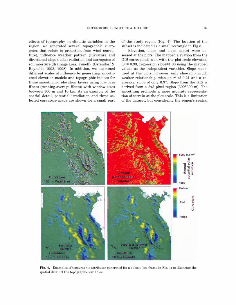
effects of topography on climatic variables in the region, we generated several topographic surro-gates that relate to protection from wind (curva-ture), influence weather pattern (curvature and directional slope), solar radiation and surrogates of soil moisture (drainage area, runoff) (Ostendorf & Reynolds 1993, 1998). In addition, we examined different scales of influence by generating smooth-ened elevation models and topographic indices for these smoothened elevation layers using low-pass filters (running-average filters) with window sizes between 300 m and 10 km. As an example of the spatial detail, potential irradiation and three se-lected curvature maps are shown for a small part

of the study region (Fig. 4). The location of the subset is indicated as a small rectangle in Fig 3.

Elevation, slope and slope aspect were as-sessed at the plots. The mapped elevation from the GIS corresponds well with the plot-scale elevation (r2 = 0.93, regression slope=1.03 using the mapped values as the independent variable). Slope meas-ured at the plots, however, only showed a much weaker relationship, with an r2 of 0.21 and a re-gression slope of only 0.37. Slope from the GIS is derived from a 3x3 pixel region (300*300 m). The smoothing prohibits a more accurate representa-tion of terrain at the plot scale. This is a limitation of the dataset, but considering the region’s spatial

Fig. 4. Examples of topographic attributes generated for a subset (see frame in Fig. 1) to illustrate the spatial detail of the topographic variables.

38 FOREST BIOMASS IN QUEENSLAND

extent of 20,000 km2, this compromise seemed ap-propriate.

Air-photo classification Air photos (at a scale of 1:25,000) were visually

interpreted. The vegetation was broadly classified based on characters including the presence or ab-sence of an understorey, canopy height and species dominance, This yielded 8 different forest types, described in detail in Harrington & Sanderson (1994).

Analysis method In order to evaluate the relative importance of

each environmental variable, we computed first one and successively multi-dimensional linear, quadratic regression and generalized additive re-gression models (GAM) using all variables listed in Table 1. Since several environmental variables are correlated with each other, we did not use auto-mated procedures such as stepwise regression, but conducted a residual analysis using a baseline model formulated using results from the univari-ate models. Categorical data are included as bi-nary dummy variables (multidimensional regres-sion). Using linear and non-linear regression methods, we can separate the linear and nonlinear effects of environmental conditions on biomass. The quadratic method was added to present re-sults from the simplest possible nonlinear method. The predictive capability is evaluated by compar-ing the percentage of deviance explained by the different models, which is equivalent to r2 values in the general linear models.

Generalized additive models are gaining promi-nence where the assumption of linearity is violated. They are non-parametric, allowing a smooth func-tion to be generated through the data cloud. For the GAM analysis we used a spline smoothing function of 3 degrees of freedom. In one dimension, the GAM with the settings used, is equivalent to a spline; in multiple dimensions, however, iterative solutions are found with additive degree of freedoms (Hastie & Tibshirani 1990).

Results and discussion

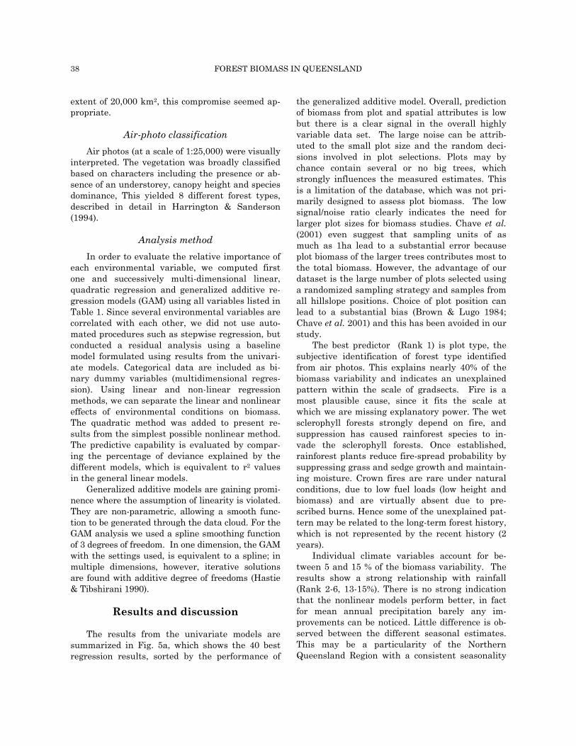
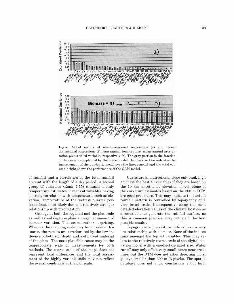
The results from the univariate models are summarized in Fig. 5a, which shows the 40 best regression results, sorted by the performance of

the generalized additive model. Overall, prediction of biomass from plot and spatial attributes is low but there is a clear signal in the overall highly variable data set. The large noise can be attrib-uted to the small plot size and the random deci-sions involved in plot selections. Plots may by chance contain several or no big trees, which strongly influences the measured estimates. This is a limitation of the database, which was not pri-marily designed to assess plot biomass. The low signal/noise ratio clearly indicates the need for larger plot sizes for biomass studies. Chave et al. (2001) even suggest that sampling units of as much as 1ha lead to a substantial error because plot biomass of the larger trees contributes most to the total biomass. However, the advantage of our dataset is the large number of plots selected using a randomized sampling strategy and samples from all hillslope positions. Choice of plot position can lead to a substantial bias (Brown & Lugo 1984; Chave et al. 2001) and this has been avoided in our study.

The best predictor (Rank 1) is plot type, the subjective identification of forest type identified from air photos. This explains nearly 40% of the biomass variability and indicates an unexplained pattern within the scale of gradsects. Fire is a most plausible cause, since it fits the scale at which we are missing explanatory power. The wet sclerophyll forests strongly depend on fire, and suppression has caused rainforest species to in-vade the sclerophyll forests. Once established, rainforest plants reduce fire-spread probability by suppressing grass and sedge growth and maintain-ing moisture. Crown fires are rare under natural conditions, due to low fuel loads (low height and biomass) and are virtually absent due to pre-scribed burns. Hence some of the unexplained pat-tern may be related to the long-term forest history, which is not represented by the recent history (2 years).

Individual climate variables account for be-tween 5 and 15 % of the biomass variability. The results show a strong relationship with rainfall (Rank 2-6, 13-15%). There is no strong indication that the nonlinear models perform better, in fact for mean annual precipitation barely any im-provements can be noticed. Little difference is ob-served between the different seasonal estimates. This may be a particularity of the Northern Queensland Region with a consistent seasonality

OSTENDORF, BRADFORD & HILBERT 39

of rainfall and a correlation of the total rainfall amount with the length of a dry period. A second group of variables (Rank 7-15) contains mainly temperature estimates or maps of variables having a strong correlation with temperature, such as ele-vation. Temperature of the wettest quarter per-forms best, most likely due to a relatively stronger relationship with precipitation.

Geology at both the regional and the plot scale as well as soil depth explain a marginal amount of biomass variation. This seems rather surprising. Whereas the mapping scale may be considered too coarse, the results are corroborated by the low in-fluence of both soil depth and soil parent material of the plots. The most plausible cause may be the inappropriate scale of measurements for both methods. The coarse scale of the maps does not represent local differences and the local assess-ment of the highly variable soils may not reflect the overall conditions at the plot scale.

Curvature and directional slope only rank high amongst the best 40 variables if they are based on the 10 km smoothened elevation model. None of the curvature estimates based on the 300 m DTM are good predictors. This may indicate that actual rainfall pattern is controlled by topography at a very broad scale. Consequently, using the most detailed elevation values of the climate location as a covariable to generate the rainfall surface, as this is common practice, may not yield the best possible results.

Topographic soil moisture indices have a very low relationship with biomass. None of the indices rank amongst the top 40 variables. This may re-late to the relatively coarse scale of the digital ele-vation model with a one-hectare pixel size. Water runoff may only affect very small zones near creek lines, but the DTM does not allow depicting moist gulleys smaller than 300 m (3 pixels). The spatial database does not allow conclusions about local

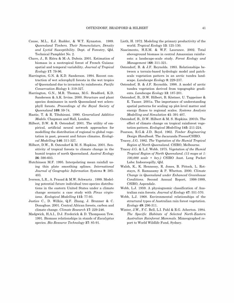
Fig 5. Model results of one-dimensional regressions (a) and three-dimensional regressions of mean annual temperature, mean annual precipi-tation plus a third variable, respectively (b). The gray portion is the fraction of the deviance explained by the linear model, the black section indicates the improvement of the quadratic model over the linear model and the total col-umn height shows the performance of the GAM-model.

40 FOREST BIOMASS IN QUEENSLAND

effects of topography-related water availability on biomass.

The analysis by multidimensional models (us-ing mean annual precipitation and temperature as a baseline model and adding successive variables) shows a general improvement (Fig. 5b) and largely corroborates the findings of the one-dimensional models related to the relative performance of vari-ables. Mean annual temperature and precipitation together explain 15, 16 and 18% for the linear, quadratic and additive models, respectively. All added variables improve the baseline model. The largest improvement is achieved by including ei-ther location (latitude and longitude) or gradsect. This indicates the existence of pattern at a broad scale that could not be explained by the environ-mental variables in the database, supporting the conclusions from the one-dimensional analysis.

The best model again includes plot vegetation type and explains 42.5% of the biomass variability. However, the improvement of 4.5% gained by add-ing rainfall and temperature to the one-dimensional model of plot type (37.9%) is lower than for most other variables. The climate layers explain relatively little additional variance. The good performance of plot type may, therefore, indi-cate that the observed vegetation pattern on air-photos may partly represent the true rainfall pat-tern. Climate station density is insufficient to cap-ture local rainfall pattern. Using the proximity to rainfall gauging stations to generate rainfall sur-faces may lead to errors, especially where the sta-tion density is low, as towards the drier areas with little agricultural potential. Precipitation for those gradsects that are close to stations of a higher ele-vation may, therefore, be overestimated. On the other hand, using detailed elevation as a covari-able may lead to errors in some valleys, where the mapped precipitation gradients follow elevation too closely and the precipitation shows much variation within a plot type. The way topography influences the regional climate appears to be little understood. It is noticeable in this context that curvature and directional slope still perform best at the 10 km scale, even with precipitation and temperature already included in the model. This also points to a systematic unexplained broad-scale influence of topography on climatic patterns.

Conclusions

Precipitation and temperature exert the strongest effect of biomass in these northern Aus-tralian forests. Soil parent material and broad categories of soil depth show lesser importance. Mapped (generalized or smoothened) vegetation types based on air-photos explain the largest amount of variance. Fire history appears to be a most important spatial variable, but historic fire patterns are not available. It is also noticeable that relatively broad patches are the best predictors. This in particular shows the importance of objec-tive spatial sampling designs for obtaining a re-gional estimates. The variability within regional climate zones is large compared to the variability within zones that can be readily identified using remote sensing methods but for which we can only guess its causes. This poses questions related to a source of error of climate estimates for plots where no long-term climate records are available directly at the site or in very close proximity.

More research related to the spatial scale of covariables used for interpolation of sparse climate station data seems necessary.

Acknowledgments

The authors gratefully acknowledge the sup-port of Graham Harrington, who initiated the field research and supported the work with many dis-cussions. The detailed suggestions of anonymous reviewers were highly appreciated.

References

Austin, M.P. & P.C. Heyligers. 1989. Vegetation survey design for conservation: gradsect sampling of forest in north-eastern New South Wales. Biological Con-servation 50: 13-32.

Austin, M.P. & P.C. Heyligers. 1991. New approach to vegetation survey design: gradsect sampling. pp. 31-36 In: C.R. Margules & M.P. Austin (ed.) Nature Conservation: Cost Effective Biological Surveys and Data Analysis. CSIRO Melbourne.

Brown L. & A.E. Lugo. 1984. Biomass of tropical forests: A new estimate based on forest volume. Science 223: 1290-1293.

Box, E.O., D.W. Crumpacker & E.D. Hardin. 1999. Pre-dicted effects of climatic change on distribution of ecologically important native tree and shrub species in Florida. Climatic Change 41: 213-248.

OSTENDORF, BRADFORD & HILBERT 41

Cause, M.L., E.J. Rudder, & W.T. Kynaston. 1989. Queensland Timbers. Their Nomenclature, Density and Lyctid Susceptibility. Dept. of Forestry, Qld. Technical Pamphlet No. 2.

Chave, J., B. Riéra & M.-A. Dubois. 2001. Estimation of biomass in a neotropical forest of French Guiana: spatial and temporal variability. Journal of Tropical Ecology 17: 79-96.

Harrington, G.N. & K.D. Sanderson. 1994. Recent con-traction of wet sclerophyll forests in the wet tropics of Queensland due to invasion by rainforests. Pacific Conservation Biology 1: 319-327.

Harrington, G.N., M.R. Thomas, M.G. Bradford, K.D. Sanderson & A.K. Irvine. 2000. Structure and plant species dominance in north Queensland wet sclero-phyll forests. Proceedings of the Royal Society of Queensland 109: 59-74.

Hastie, T. & R. Tibshirani. 1990. Generalized Additive Models. Chapman and Hall, London.

Hilbert, D.W. & B. Ostendorf. 2001. The utility of em-pirical, artificial neural network approaches for modelling the distribution of regional to global vege-tation in past, present and future climates. Ecologi-cal Modelling 146: 311-327.

Hilbert, D.W., B. Ostendorf & M. S. Hopkins. 2001. Sen-sitivity of tropical forests to climate change in the humid tropics of north Queensland. Austral Ecology 26: 590-603.

Hutchinson M.F. 1995. Interpolating mean rainfall us-ing thin plate smoothing splines. International Journal of Geographic Information Systems 9: 385-403.

Iverson, L.R., A. Prasad & M.W. Schwartz . 1999. Model-ing potential future individual tree-species distribu-tions in the eastern United States under a climate change scenario: a case study with Pinus virgin-iana. Ecological Modelling 115: 77-93.

Justice C., D. Wilkie, Q.F. Zhang, J. Brunner & C. Donoghue. 2001. Central African forests, carbon and climate change. Climate Research 17: 229-246.

Madgwick, H.A.I., D.J. Frederick & D. Thompsson Tew. 1991. Biomass relationships in stands of Eucalyptus species. Bio-Resource Technology 37: 85-91.

Lieth, H. 1972. Modeling the primary productivity of the world. Tropical Ecology 13: 125-130.

Nascimento, H.E.M. & W.F. Laurance. 2002. Total aboveground biomass in central Amazonian rainfor-ests: a landscape-scale study. Forest Ecology and Management 168: 311-321.

Ostendorf, B. & J.F. Reynolds. 1993. Relationships be-tween a terrain-based hydrologic model and patch-scale vegetation pattern in an arctic tundra land-scape. Landscape Ecology 8: 229-237.

Ostendorf, B. & J.F. Reynolds. 1998. A model of arctic tundra vegetation derived from topographic gradi-ents. Landscape Ecology 13: 187-201.

Ostendorf, B., D.W. Hilbert, B. Köstner, U. Tappeiner & E. Tasser. 2001a. The importance of understanding spatial patterns for scaling up plot-level matter and energy fluxes to regional scales. Systems Analysis Modelling and Simulation 41: 391-407.

Ostendorf, B., D.W. Hilbert & M. S. Hopkins. 2001b. The effect of climate change on tropical rainforest vege-tation pattern. Ecological Modelling 145: 211-224.

Pearson, R.G.& J.D. Boyd. 1962. Timber Engineering Design Handbook. The Jacaranda Preess/CSIRO.

Tracey, J.G. 1982. The Vegetation of the Humid Tropical Region of North Queensland. CSIRO, Melbourne.

Tracey J.G. & L.J. Webb. 1975. Vegetation of the Humid Tropical Region of North Queensland. (15 maps at 1: 100,000 scale + key.) CSIRO Aust. Long Pocket Labs: Indooroopilly, Qld.

Walsh, K., K. Hennessy, R. Jones, B. Pittock, L. Rot-stayn, S. Ramasamy & P. Whetton. 2000. Climate Change in Queensland under Enhanced Greenhouse Conditions. Second Annual Report, 1998-1999, CSIRO, Aspendale.

Webb, L.J. 1959. A physiognomic classification of Aus-tralian rain forests. Journal of Ecology 47: 551-570.

Webb, L.J. 1968. Environmental relationships of the structural types of Australian rain forest vegetation. Ecology 49: 296-311.

Winter, J.W., F.C. Bell, L.I. Pahl & R.G. Atherton. 1984. The Specific Habitats of Selected North-Eastern Australian Rainforest Mammals. Mimeographed re-port to World Wildlife Fund, Sydney.