REFLECTANCE-BASED PULSE OXIMETER FOR THE … · In this project, a reflectance-based pulse oximeter was ... which transmittance based pulse oximetry cannot ... components and a programmed

REFLECTANCE-BASED PULSE OXIMETER

FOR THE CHEST AND WRIST

A Major Qualifying Project Report:

Submitted to the Faculty

Of the

WORCESTER POLYTECHNIC INSTITUTE

In partial fulfillment of the requirements for the

Degree of Bachelor of Science

By

_________________________________________

Alexandra Fontaine

_________________________________________

Arben Koshi

_________________________________________

Danielle Morabito

_________________________________________

Nicolas Rodriguez

Submitted on:

Approved by:

________________________________________________________________

Professor Yitzhak Mendelson, Advisor, Dept. of Biomedical Engineering

i

Authorship

Section Author

Introduction Nicolas Rodriguez, Danielle Morabito, Alex

Fontaine, Arben Koshi

Literature Review Nicolas Rodriguez, Danielle Morabito, Alex

Fontaine, Arben Koshi

Design Approach Alex Fontaine, Danielle Morabito

Device Development Nicolas Rodriguez, Danielle Morabito

Methods Nicolas Rodriguez, Danielle Morabito

Final Design Arben Koshi, Nicolas Rodriguez, Danielle

Morabito

Results Alex Fontaine, Arben Koshi

Discussion Arben Koshi, Alex Fontaine

Summary Arben Koshi

Conclusion Arben Koshi

Future Improvements Arben Koshi, Nicolas Rodriguez

Appendix A Danielle Morabito

Appendix B Arben Koshi

Appendix C Alex Fontaine

Appendix D Arben Koshi

ii

Abstract Reflectance-based pulse oximetry is a technique used for noninvasively monitoring the oxygen saturation

(SpO2) and pulse rate (PR). However, there is little supporting evidence that it can accurately collect

measurements from the chest and wrist. In this project, a reflectance-based pulse oximeter was built and

used to collect measurements while sitting, standing, during self-induced hypoxia, and during self-

induced hyperventilation then compared to the measurements taken by a HOMEDIC Deluxe Pulse

Oximeter. The prototype was able to accurately measure within an error of + 1% and ±3% for SpO2 and

PR respectively from the wrist while an error of ±1% and +4% for SpO2 and PR respectively from the

chest.

iii

Acknowledgements We would like to thank Professor Mendelson for advising this project. We would also like to

acknowledge Dr. Adriana Hera and Lisa Wall for their support.

iv

Executive Summary Oxygen saturation (SpO2) is the measurement of oxyhemoglobin (HbO2) in arterial blood. SpO2 is an

important vital measurement because it shows the levels of blood oxygenation. Traditionally, SpO2 is

measured by invasively drawing blood samples. This method, however, is not ideal and it is unable to

provide clinicians with real-time measurements. With the need for a noninvasive way to measure SpO2,

pulse oximetry was developed. The use of this technology allows clinicians to determine SpO2 in patients

that are sedated, anesthetized, unconscious, or unable to regulate their own oxygen supply.

Reflectance-based pulse oximetry allows measurements to be taken from areas of the body in

which transmittance based pulse oximetry cannot be applied. In reflectance-based pulse oximetry, the

incident light is passed through the skin and is reflected off the subcutaneous tissue and bone. To this day,

being able to measure signals from the chest and wrist with one single device has not been successfully

achieved. Such a device would allow patients to measure SpO2 and pulse rate (PR) without hindering

their normal day-to-day activities.

The prototype pulse oximeter constructed during this project consists of two hardware

components and a programmed LabVIEW Virtual Instrument (VI). The hardware components consist of

the sensor and a circuit which produces, collects, and processes photoplethysmographic (PPG) signals.

The VI collects the PPG signals produced by the hardware and process them in order to produce

numerical results for PR and SpO2 . The optical sensor is made up of two Light Emitting Diodes (LEDs),

a red LED, with a peak emission wavelength of 660 nm, and an infrared emitter with a peak emission

wavelength of 940 nm. These LEDs are positioned next to each other in the center of a circular Printed

Circuit Board (PCB) and surrounded by 8 photodiodes (PD). The circuitry for the sensor consists of an

Arduino Duo Microprocessor which is programmed to light up the red and infrared LEDs intermittently at

a frequency of 100Hz. The PDs are connected in photovoltaic mode in order to produce a voltage output.

Operational amplifiers are utilized to amplify the photodiode output. Once amplified, the red and infrared

PPG signals obtained from the photodetectors are sent through two Sample-and-Hold circuits to separate

the signals into their respective alternating current (AC) and direct current (DC) components for further

filtering and amplification.

The four input signals sent to the LabVIEW software : AC red, AC infrared, DC red and DC

infrared access the VI via a National Instruments (NI) Data Acquisition (DAQ) system. The AC

components of the red and infrared PPGs are measured using a peak-to-peak detection algorithm, while

the DC components are measured by finding their respective averages. Once the signals are processed,

SpO2 is calculated by obtaining the ratio of the AC and DC components of the red PPG and dividing that

by the ratio of the AC and DC components of the infrared PPG. To calculate PR, the frequency of the

infrared AC signal is measured using frequency measurement parameters in LabVIEW and then

v

multiplied by 60 to display PR in beats per minute (bpm). To compare the measurants taken from the

pulse oximeter prototype, a transmission-type finger HOMEDICS Deluxe Pulse Oximeter was utilized as

reference. The reliability of the Deluxe Pulse Oximeter was tested against a Biopac ECG model 100C

module and was concluded that the HOMEDICS Deluxe Pulse Oximeter was provided accurate enough

measurements for pulse rate.

For testing, the sensor was strapped to the wrist and chest of each subject using a Velcro strap

while the HOMEDICS Deluxe Pulse Oximeter was placed on the subject’s index finger. The VI was set

up to collect, average and display SpO2 and PR data every 10 seconds throughout a 6 minute timespan

accounting for 36 measurements. At this point, a second individual that was monitoring the reference

device recorded the corresponding SpO2 and PR values displayed by the HOMEDICS pulse oximeter.

Subjects were tested on the chest and wrist while sitting, standing, during self-induced hyperventilation,

and during self-induced hypoxia.

While collecting data, it was noticed that the PR measurements collected from the chest had

significantly larger margins of error compared to those from the wrist. One possible explanation for this

discrepancy deals with the LabVIEW algorithm for PR calculation. Instead of doing peak-peak analysis,

we opted to use a search tool which graphs a power spectrum of the data and searches for the highest

amplitude frequency between 0.75Hz and 2.25Hz. This method is very effective at PR values ranging

between 45 and 135 bpm, but loses its accuracy at higher PR values. Measurements above 135 bpm were

detected by the reference, but not accurately detected by the prototype.

Margins of error obtained from the standing and sitting measurement tests on the wrist included

0.6%, and 0.2% for SpO2 and 0.2%, 1.1% for PR respectively. Measurements from the chest displayed

errors of 0.4% and 0.3% for SpO2 and 0.1%, and 0.7% for PR while standing and sitting respectively.

Based on this data, our prototype for a reflectance-based pulse oximeter for the chest and wrist was

successful in measuring PR and SpO2.

vi

Table of Contents

Authorship.................................................................................................................................................................. i

Abstract ...................................................................................................................................................................... ii

Acknowledgements ............................................................................................................................................... iii

Executive Summary .............................................................................................................................................. iv

Table of Figures .................................................................................................................................................. viii

Table of Tables ........................................................................................................................................................ x

Abbreviations .......................................................................................................................................................... xi

1 Introduction .................................................................................................................................................. 12

2 Literature Review ....................................................................................................................................... 13

Oxygen Saturation .............................................................................................................................. 13 2.1

Pulse Oximetry .................................................................................................................................... 13 2.2

2.2.1 Principle of a Pulse Oximeter ................................................................................................ 15

2.2.2 Methods of Light Detection .................................................................................................... 16

2.2.3 Photoplethysmogram ................................................................................................................ 17

2.2.4 Wavelength Optimization ....................................................................................................... 17

2.2.5 Limitations and Applications of Pulse Oximetry ............................................................. 17

Reflectance vs. Transmittance Pulse Oximetry ......................................................................... 18 2.3

New Studies for Pulse Oximeters .................................................................................................. 19 2.4

3 Design Approach ........................................................................................................................................ 21

Initial Client Statement ..................................................................................................................... 21 3.1

Clinical Need ....................................................................................................................................... 21 3.2

Design Parameters .............................................................................................................................. 21 3.3

3.3.1 Objectives .................................................................................................................................... 21

3.3.2 Constraints ................................................................................................................................... 22

3.3.3 Functions ...................................................................................................................................... 22

3.3.4 Design Specifications ............................................................................................................... 23

Revised Client Statement ................................................................................................................. 25 3.4

4 Device Development ................................................................................................................................. 27

Device Alternatives............................................................................................................................ 27 4.1

4.1.1 Sensor Design 1.......................................................................................................................... 27

4.1.2 Sensor Design 2.......................................................................................................................... 28

Software Design .................................................................................................................................. 29 4.2

5 Methods ......................................................................................................................................................... 30

vii

Photodetection Unit ........................................................................................................................... 30 5.1

PPG ......................................................................................................................................................... 30 5.2

Filter Design ........................................................................................................................................ 30 5.3

Software ................................................................................................................................................ 31 5.4

5.4.1 Incoming Signals ....................................................................................................................... 32

5.4.2 Filtering ........................................................................................................................................ 34

5.4.3 Frequency of Pulse Rate .......................................................................................................... 35

5.4.4 Pulse Rate Calculation ............................................................................................................. 36

5.4.5 Spectral Measurements ............................................................................................................ 37

5.4.6 SpO2 Calculation ........................................................................................................................ 39

5.4.7 Preliminary VI Test ................................................................................................................... 44

Experimentation/Testing .................................................................................................................. 48 5.5

6 Final Design ................................................................................................................................................. 51

Device Hardware ................................................................................................................................ 51 6.1

6.1.1 Sensor ............................................................................................................................................ 51

6.1.2 Circuitry ........................................................................................................................................ 52

Software ................................................................................................................................................ 56 6.2

7 Results ........................................................................................................................................................... 59

Comparison Graphs ........................................................................................................................... 61 7.1

Dynamic Response Plots .................................................................................................................. 73 7.2

Residual Plots ...................................................................................................................................... 91 7.3

8 Discussion..................................................................................................................................................... 98

10 Summary ..................................................................................................................................................... 101

11 Conclusion .................................................................................................................................................. 103

12 Future Improvements .............................................................................................................................. 104

References ............................................................................................................................................................ 106

Appendix A: Description of LabVIEW ....................................................................................................... 107

Appendix B: Bill of Materials ........................................................................................................................ 117

Appendix C: Data Sets ..................................................................................................................................... 118

Appendix D: Filter Bode Plots ....................................................................................................................... 128

viii

Table of Figures Figure 2.1: Arterial blood changing over time, PPG

[11] .................................................................................................................. 14 Figure 2.2: Optical absorption spectra of Hb, HbO2, MetHb, and BbCO

[11] ........................................................................... 15 Figure 2.3: Transmittance pulse oximetry ............................................................................................................................................. 18 Figure 2.4: Reflectance pulse oximetry ................................................................................................................................................... 18 Figure 2.5: Forehead pulse oximeter ....................................................................................................................................................... 19 Figure 3.1: Objective tree ............................................................................................................................................................................ 22 Figure 5.1: Unfiltered output of a PPG signal with an AC component riding on top of a DC component ..................... 30 Figure 5.2: Configuration of functions to separate incoming signals .......................................................................................... 33 Figure 5.4: Filter function and graph ...................................................................................................................................................... 35 Figure 5.5: Tone measurements output frequency .............................................................................................................................. 35 Figure 5.6: Configure tone measurements parameters ..................................................................................................................... 36 Figure 5.7: Functions used to calculate pulse rate ............................................................................................................................. 37 Figure 5.8: Amplitude and level measurements functions with numeric indicators ................................................................ 38 Figure 5.9: Configure amplitude and level measurements set to mean (DC) ............................................................................ 39 Figure 5.10: SpO2 calculation .................................................................................................................................................................... 40 Figure 5.11: The configuration of function that limit the displayed SpO2 .................................................................................. 41 Figure 5.12: VI Block Diagram ................................................................................................................................................................. 42 Figure 5.13: VI Front Panel........................................................................................................................................................................ 43 Figure 5.14: Front panel for the simulated hypoxia test with low amplitude ............................................................................ 45 Figure 5.15: Front panel for the simulated hypoxia test with high amplitude .......................................................................... 46 Figure 5.16: Block diagram for the simulated hypoxia test ............................................................................................................. 47 Figure 5.17: Application of the sensor to the wrist (left) and the chest (right) ......................................................................... 49 Figure 6.1: Top View of sensor module with photodiodes and LEDs. ......................................................................................... 51 Figure 6.2: Platform view of sensor module ......................................................................................................................................... 52 Figure 6.3: Block diagram of the prototype pulse oximeter ............................................................................................................ 53 Figure 6.4:LED driver timing diagram with 2.5ms time increments ............................................................................................ 54 Figure 6.5: Circuit design for pulse oximeter device ......................................................................................................................... 55 Figure 6.6: Block Diagram of Final VI ................................................................................................................................................... 57 Figure 6.7: Front Panel of Final VI ......................................................................................................................................................... 58 Figure 7.1: Example of corrupted PPG .................................................................................................................................................. 60 Figure 7.2: Comparison graph for the chest sitting tests. The solid line represents the regression line and the dashed

line represents the identity line. ................................................................................................................................................................. 62 Figure 7.3: Comparison graph for the chest standing tests. The solid line represents the regression line and the

dashed line represents the identity line. .................................................................................................................................................. 64 Figure 7.4: Comparison graph for the wrist sitting tests. The solid line represents the regression line and the dashed

line represents the identity line. ................................................................................................................................................................. 66 Figure 7.5: Comparison graph for the wrist standing tests. The solid line represents the regression line and the

dashed line represents the identity line. .................................................................................................................................................. 68 Figure 7.6: Comparison graph for hyperventilation tests ................................................................................................................ 70 Figure 7.7: Comparison graph for hypoxia tests. The solid line represents the regression line and the dashed line

represents the identity line. .......................................................................................................................................................................... 72 Figure 7.8: Oxygen saturation measurement validation plot for the chest standing test ...................................................... 74 Figure 7.9: Pulse rate measurement validation plot for the chest standing test ....................................................................... 75 Figure 7.10: Oxygen saturation measurement validation plot for the chest sitting test ......................................................... 77 Figure 7.11: Pulse rate measurement validation plot for the chest sitting test ......................................................................... 78 Figure 7.12: Pulse rate measurement validation plot 1 for hyperventilation test .................................................................... 80 Figure 7.13: Pulse rate measurement validation plot 2 for hyperventilation test .................................................................... 81 Figure 7.14: Pulse rate measurement validation plot for the wrist sitting test ......................................................................... 83 Figure 7.15: Oxygen saturation measurement validation plot for the wrist sitting test ......................................................... 84 Figure 7.16: Oxygen saturation measurement validation plot for the wrist standing test .................................................... 86 Figure 7.17: Pulse rate measurement validation plot for the wrist standing test ..................................................................... 87 Figure 7.18: Oxygen saturation measurement validation plot 1 for hypoxia test .................................................................... 89

ix

Figure 7.19: Oxygen saturation measurement validation plot 2 for hypoxia test .................................................................... 90 Figure 7.20: Residual plot for hyperventilation testing for data set 1 (dotted lines: + 2SD, solid line: average of

differences) ........................................................................................................................................................................................................ 92 Figure 7.21: Residual plot for hyperventilation testing for data set 2(dotted lines: + 2SD, solid line: average of

differences) ........................................................................................................................................................................................................ 93 Figure 7.22: Residual plot for hyperventilation testing for data set 3 (dotted lines: + 2SD, solid line: average of

differences) ........................................................................................................................................................................................................ 94 Figure 7.23: Residual plot for hypoxia testing for data set 1 (dotted lines: + 2SD, solid line: average of differences)

............................................................................................................................................................................................................................... 96 Figure 7.24: Residual plot for hypoxia testing for data set 2 (dotted lines: + 2SD, solid line: average of differences)

............................................................................................................................................................................................................................... 97

x

Table of Tables Table 3.1: Respironic's WristOx Ambulatory Finger Pulse Oximeter Specifications

[21] ...................................................... 23 Table 3.2: Santa Medical's Finger Pulse Oximeter Specifications

[7]............................................................................................ 24 Table 3.3: Crucial Medical Systems Finger Pulse Oximeter Specifications

[22]........................................................................ 24 Table 3.4: Project Specifications ............................................................................................................................................................... 25 Table 7.1: Calculated accuracy for the average SpO2 and PR for each data set ..................................................................... 59 Table 7.2: Prototype accuracy based on all data collected ............................................................................................................. 60

xi

Abbreviations O2: Oxygen

Hb: Hemoglobin

HbO2: Oxyhemoglobin

SpO2: Oxygen saturation

SaO2: Oxygen saturation measured invasively

PR: Pulse rate

COHb: Carboxyhemoglobin

MetHb: Methyl hemoglobin

PPG: Photoplethysmogram

VI: Virtual Instrument

12

1 Introduction One of the most important elements needed to sustain life is oxygen (O2) because it is used by cells to

turn sugars into useable energy. Oxyhemoglobin (HbO2) is the protein hemoglobin, found in red blood

cells, bounded to O2 that delivers 98% of oxygen to cells. The measurement and calculation of the

percentage of HbO2 in arterial blood is known as oxygen saturation (SpO2). [1]

Originally, SpO2 was measured by taking samples of blood and measuring O2 levels directly. This

method was invasive and was unable to provide real-time measurements. This measuring technique made

it impossible for SpO2 to be recognized as an important measure of wellness until a non-invasive method

of measuring SpO2 in real-time was established. [2]

The need for a non-invasive method of measuring SpO2 in real-time led to the development of

pulse oximetry. Pulse oximetry derives SpO2 and pulse rate (PR) from a photoplethysmogram (PPG). The

PPG is obtained by measuring changes in light absorbed by the blood. Red and infrared wavelengths are

used to obtain the PPG because these wavelengths are easily transmitted through tissues, allowing SpO2

to be calculated from the ratio of the absorption of the red and infrared light.

The first device used to continuously measure blood oxygen saturation of human blood in vivo

(SaO2) was built by Karl Matthes in 1935. [2]

However, it was not until 1983 that William New and Mark

Yelderman, after recognizing the need of an accurate oximeter in the operating room evaluated and

produced the pulse oximeter with aims to make it an intraoperative monitoring device. [2]

Pulse oximetry

allows for an accurate determination of O2 levels in patients that are sedated, anesthetized, unconscious,

and unable to regulate their own oxygen supply as well as provides information needed to avoid

irreversible tissue damage. [2]

Since the invention of pulse oximetry, the measurement of SpO2 has become an important part of the

medical world. Nevertheless, improvements such as the application of the reflectance-based technique to

measure SpO2 from multiple locations on the body are still to be developed. This project demonstrates the

use of reflectance-based pulse oximetry to obtain measurements for PR and SpO2 from the chest and

wrist. This development in pulse oximetry technology will pave the way for the development of new and

novel pulse oximeters that can be worn as accessories, are easily concealed under clothing, and more

acclimated to use outside of hospital settings.

13

2 Literature Review This is a thorough literature review covering the necessary background needed to fully understand this

project.

Oxygen Saturation 2.1SpO2 is the amount of O2 that is carried in the blood. In the human body, SpO2 is defined as the ratio of

HbO2 to the total concentration of Hb (reduced Hb + HbO2) present in the blood [1]

.

( )

(1)

Hb is the iron-containing protein in red blood cells that transports O2 to the tissues. This protein

forms an unstable and reversible bond with O2. Thus, Hb in its oxygenated state is called HbO2 and

exhibits a bright red color. Conversely, in its reduced state, it exhibits a purplish blue color [3]

. Hb can

carry up to four O2 molecules.

In calculating the absorption of light at a specific wavelength by a homogeneous substance, the

Beer-Lambert law can be used to show the basic relationship between the transmitted light intensity and

the incident light:

(2)

where ‘It’ is the intensity of transmitted light, ‘Io’ is incident light intensity, ‘ε’ is the extinction

coefficient (fraction of light absorbed at a specific wavelength), ‘c’ is the concentration of the sample, and

‘d’ is the length of the light path through the sample. However, this is difficult to use in pulse oximetry

because the light scattering through the tissue cannot be distinguished from that of blood [1]

.

Two independent equations can be derived to describe the absorption of light by both Hb and

HbO2 at two distinct wavelengths. These equations can then be solved to find the concentration of Hb and

HbO2 in blood and establish the relationship,

( )

( ) (3)

where A and B are functions of the extinction coefficients of Hb and HbO2 while ‘OD’ is the optical

density or the log(Io/It). The relationship above is the underlying principle used by commercial pulse

oximeters to measure SpO2. [1]

Pulse Oximetry 2.2Pulse oximetry was initially intended for monitoring hospitalized patients after surgery. However, after

recognizing the importance of an accurate oximetry device during surgery in operating rooms, non-

invasive pulse oximetry became a standard for anesthesiologists for intraoperative monitoring since 1990.

By the use of this technique, physicians can determine the SpO2 in patients that are sedated, anesthetized,

14

unconscious, and unable to regulate their own oxygen supply avoiding irreversible tissue damage [2]

.

It is not until 1935 that Karl Matthes used red and infrared wavelengths to build a device that

continuously measured SaO2 in vivo. Matthes stated that “the red light can pass through HbO2, but

reduced Hb absorbs it” [2]

. Non-invasive oximetry evolved even further when Robert Brinkman and

William Ziilstra began measuring SpO2 from the forehead with the use of reflected light. Brinkman and

Zijlstra made an additional modification when they divided the red signal by the infrared signal to show

continuous measurements of SpO2 [2,4]

. However, differentiating various types of Hb was still a problem.

This is when Robert Shaw invented an absolute reading ear oximeter in 1964. This device used eight

different wavelengths to identify the separate Hb species present in the blood. Although expensive, this

instrument was accurate down to 70% of SpO2 and it was commercialized for use in physiology

laboratories for pulmonary and cardiac applications. [2]

In 1970, research performed by Takuo Aoyagi and

his associates on dye-dylution techniques for measuring cardiac output led to the development of

photoplethysmogram (PPG) ,which optically generates time dependent volumetric changes in living

tissues leading to the development of pulse oximeter [1, 2]

. Here, the time dependent changes are associated

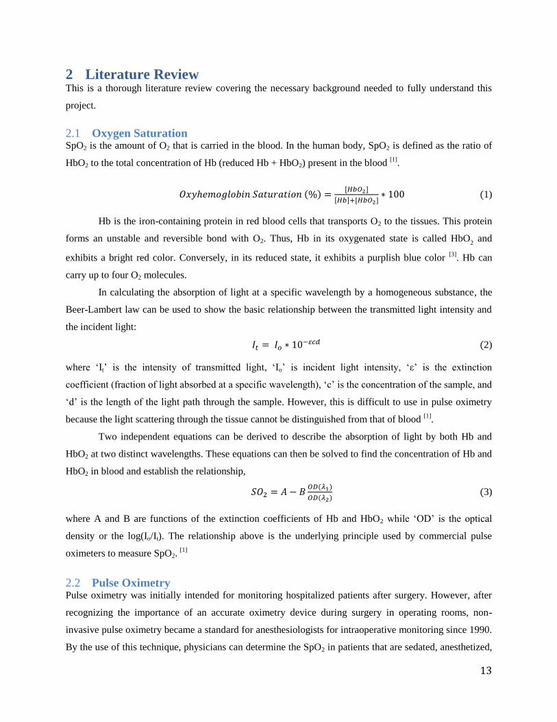
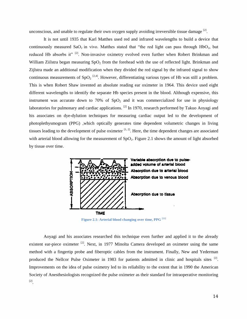
with arterial blood allowing for the measurement of SpO2. Figure 2.1 shows the amount of light absorbed

by tissue over time.

Figure 2.1: Arterial blood changing over time, PPG [11]

Aoyagi and his associates researched this technique even further and applied it to the already

existent ear-piece oximeter [2]

. Next, in 1977 Minolta Camera developed an oximeter using the same

method with a fingertip probe and fiberoptic cables from the instrument. Finally, New and Yederman

produced the Nellcor Pulse Oximeter in 1983 for patients admitted in clinic and hospitals sites [2]

.

Improvements on the idea of pulse oximetry led to its reliability to the extent that in 1990 the American

Society of Anesthesiologists recognized the pulse oximeter as their standard for intraoperative monitoring

[2].

15

2.2.1 Principle of a Pulse Oximeter A noninvasive pulse oximeter relies on an optical sensor to detect SpO2 and PR. This optical sensor is

made up of a red and an infrared LED as well as silicone photodiodes (PD) [5]

. In order to obtain SpO2,

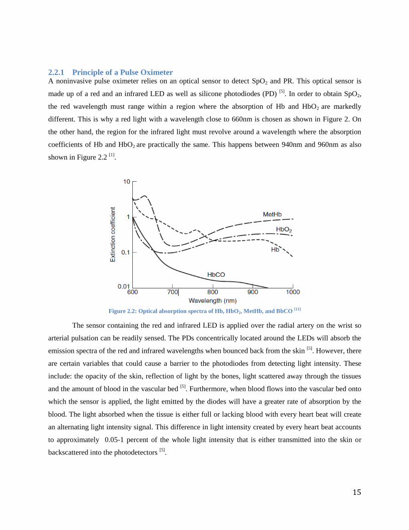
the red wavelength must range within a region where the absorption of Hb and HbO2 are markedly

different. This is why a red light with a wavelength close to 660nm is chosen as shown in Figure 2. On

the other hand, the region for the infrared light must revolve around a wavelength where the absorption

coefficients of Hb and HbO2 are practically the same. This happens between 940nm and 960nm as also

shown in Figure 2.2 [1]

.

Figure 2.2: Optical absorption spectra of Hb, HbO2, MetHb, and BbCO [11]

The sensor containing the red and infrared LED is applied over the radial artery on the wrist so

arterial pulsation can be readily sensed. The PDs concentrically located around the LEDs will absorb the

emission spectra of the red and infrared wavelengths when bounced back from the skin [5]

. However, there

are certain variables that could cause a barrier to the photodiodes from detecting light intensity. These

include: the opacity of the skin, reflection of light by the bones, light scattered away through the tissues

and the amount of blood in the vascular bed [5]

. Furthermore, when blood flows into the vascular bed onto

which the sensor is applied, the light emitted by the diodes will have a greater rate of absorption by the

blood. The light absorbed when the tissue is either full or lacking blood with every heart beat will create

an alternating light intensity signal. This difference in light intensity created by every heart beat accounts

to approximately 0.05-1 percent of the whole light intensity that is either transmitted into the skin or

backscattered into the photodetectors [5]

.

16

A pulse oximeter consists of a circuit that features a microprocessor used to light up the red and

infrared LEDs one at a time in a synchronous manner, so that when the red light is turned on the infrared

LED is turned off and vice versa [1]

. With the use of sample-and-hold circuits, the overlapped signal

acquired by the photodetector can be split into two different analog channels that correspond to the red

and infrared PPGs [1]

. The red and infrared PPG signals can be further amplified through the

implementation of high and a low pass filters so that the AC and DC components for each PPG signal can

be obtained [1]

. The new four signals can be processed through a virtual instrument (VI) designed in a

software program or a virtual instrument that calculates the ratio of AC red and DC red components and

divides it by the ratio of AC infrared and DC infrared to produce SPO2.

2.2.2 Methods of Light Detection As previously discussed, pulse oximetry relies on the PPG signals produced by the difference in the

amount of arterial blood, which in turn depends on the systolic and diastolic movements of the heart.

Measurement of light by the photodetectors can be performed either in transmission or reflection modes.

When the PPG is measured through transmission, the light source and the photodetectors are placed on

opposite sides of the vascular bed so that the light travels across the pulsating blood. Thus, this method is

limited to earlobes, feet, and fingertips. On the other side, reflectance pulse oximetry measures PPG

signals with LEDs and photodetectors placed on the same side of the sensor surface. This method allows

measurements to be taken from body parts where the transmission method cannot be used, for example on

the chest, wrist, and forehead. [6]

2.2.2.1 Distance Between LED and Photodiode In 1988, the effects of separation between the source and detector were studied

[5]. Although it is

understood that the farther away the photodiode and LED are from each other that the readings will

degrade, it was demonstrated that larger PPGs can be detected by mounting the photodiode further from

the LED. However, the tradeoff is that higher LED driving currents are required in order to overcome the

absorption of incident light due to a longer optical path length. Mendelson also shows that by mounting

more than one photodiode, a greater fraction of backscattered light can be collected and larger PPGs can

be recorded. [5]

Furthermore, in 2010, there was a similar conclusion regarding the gap sizes between the LEDs

and the photodiodes [7]

. It was found that the amount of light backscattered from the skin on the optical

module and that was absorbed by the PDs was directly proportional to the number of PDs surrounding the

LEDs. Thus, the more PDs, the more light would be absorbed.[8]

This research showed that 7mm was the

optimal distance between the LED and PD and produced the highest AC signal. Similar to Mendelson’s

17

research above, a higher current output obtained from a larger number of PDs was required in order to

obtain a stronger AC components.

2.2.3 Photoplethysmogram PPG is an optical measurement used to represent the volume of blood in vessels used to compute SpO2

and PR based on the light absorbance of blood. During the cardiac cycle, the amount of blood in tissue

varies in relation to each heartbeat, so a PPG signal is an optical representation of the cardiac cycle wave.

This results in a distinguishable AC component. The PPG is usually taken at peripheral sites such as the

finger, ear, or forehead. Since skin is perfused by blood, conventional pulse oximeters monitor the

perfusion of blood in the dermis and subcutaneous tissue of the skin. The AC component of the oximeter

signal is attributed to variation in blood volume and the DC component of the oximeter signal is generally

attributed to skin tissue absorption. [9;10;11]

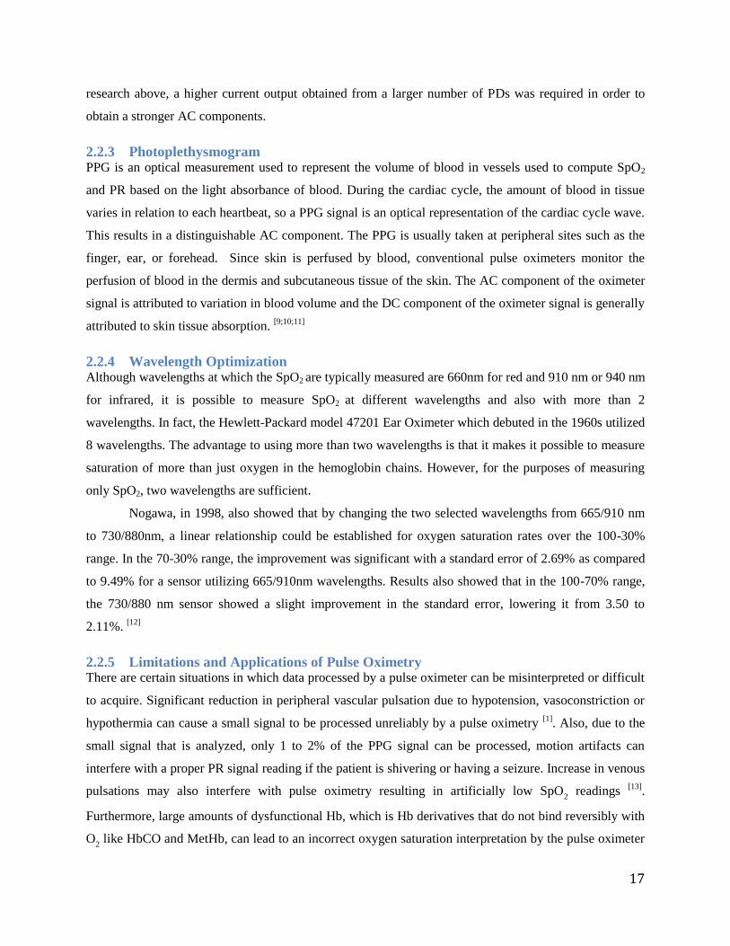
2.2.4 Wavelength Optimization Although wavelengths at which the SpO2 are typically measured are 660nm for red and 910 nm or 940 nm

for infrared, it is possible to measure SpO2 at different wavelengths and also with more than 2

wavelengths. In fact, the Hewlett-Packard model 47201 Ear Oximeter which debuted in the 1960s utilized

8 wavelengths. The advantage to using more than two wavelengths is that it makes it possible to measure

saturation of more than just oxygen in the hemoglobin chains. However, for the purposes of measuring

only SpO2, two wavelengths are sufficient.

Nogawa, in 1998, also showed that by changing the two selected wavelengths from 665/910 nm

to 730/880nm, a linear relationship could be established for oxygen saturation rates over the 100-30%

range. In the 70-30% range, the improvement was significant with a standard error of 2.69% as compared

to 9.49% for a sensor utilizing 665/910nm wavelengths. Results also showed that in the 100-70% range,

the 730/880 nm sensor showed a slight improvement in the standard error, lowering it from 3.50 to

2.11%. [12]

2.2.5 Limitations and Applications of Pulse Oximetry There are certain situations in which data processed by a pulse oximeter can be misinterpreted or difficult

to acquire. Significant reduction in peripheral vascular pulsation due to hypotension, vasoconstriction or

hypothermia can cause a small signal to be processed unreliably by a pulse oximetry [1]

. Also, due to the

small signal that is analyzed, only 1 to 2% of the PPG signal can be processed, motion artifacts can

interfere with a proper PR signal reading if the patient is shivering or having a seizure. Increase in venous

pulsations may also interfere with pulse oximetry resulting in artificially low SpO2 readings

[13].

Furthermore, large amounts of dysfunctional Hb, which is Hb derivatives that do not bind reversibly with

O2 like HbCO and MetHb, can lead to an incorrect oxygen saturation interpretation by the pulse oximeter

18

[1]. Compromised blood circulation, excessive contact pressure or weak PPG signals resulting from

insufficient contact pressures may also yield to measurement errors [14]

. Finally, one of the greatest

limitations of transmittance pulse oximetry is movement of the patient. By being attached to the finger

and the fact that extraneous movements can cause a change in absorbance of light by arterial blood flow,

a conventional pulse oximeter hinders the user to perform regular daily activities [14;15]

.

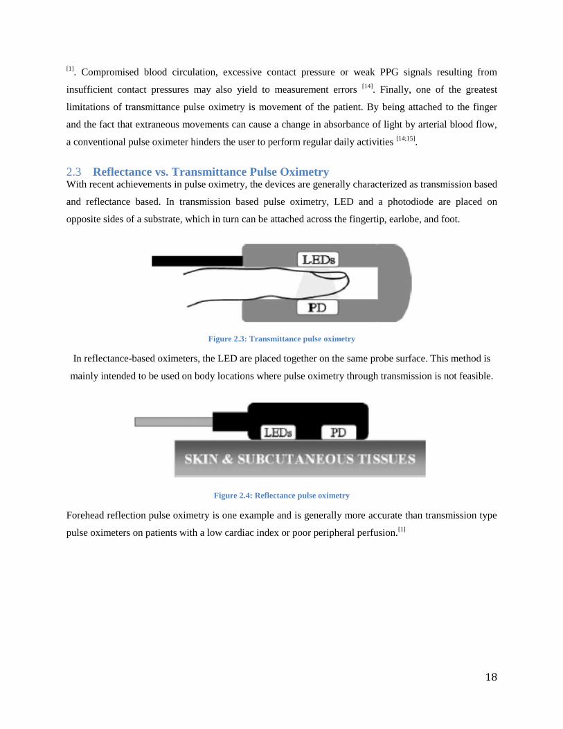
Reflectance vs. Transmittance Pulse Oximetry 2.3With recent achievements in pulse oximetry, the devices are generally characterized as transmission based

and reflectance based. In transmission based pulse oximetry, LED and a photodiode are placed on

opposite sides of a substrate, which in turn can be attached across the fingertip, earlobe, and foot.

Figure 2.3: Transmittance pulse oximetry

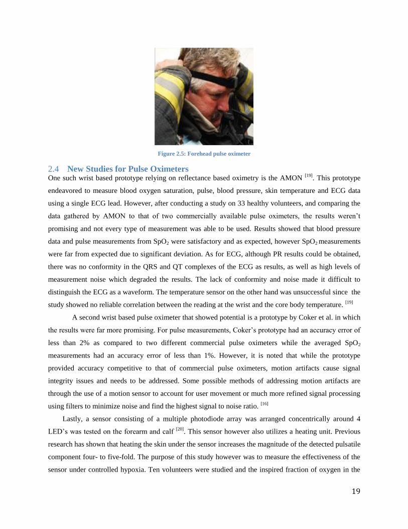
In reflectance-based oximeters, the LED are placed together on the same probe surface. This method is

mainly intended to be used on body locations where pulse oximetry through transmission is not feasible.

Figure 2.4: Reflectance pulse oximetry

Forehead reflection pulse oximetry is one example and is generally more accurate than transmission type

pulse oximeters on patients with a low cardiac index or poor peripheral perfusion.[1]

19

Figure 2.5: Forehead pulse oximeter

New Studies for Pulse Oximeters 2.4One such wrist based prototype relying on reflectance based oximetry is the AMON

[19]. This prototype

endeavored to measure blood oxygen saturation, pulse, blood pressure, skin temperature and ECG data

using a single ECG lead. However, after conducting a study on 33 healthy volunteers, and comparing the

data gathered by AMON to that of two commercially available pulse oximeters, the results weren’t

promising and not every type of measurement was able to be used. Results showed that blood pressure

data and pulse measurements from SpO2 were satisfactory and as expected, however SpO2 measurements

were far from expected due to significant deviation. As for ECG, although PR results could be obtained,

there was no conformity in the QRS and QT complexes of the ECG as results, as well as high levels of

measurement noise which degraded the results. The lack of conformity and noise made it difficult to

distinguish the ECG as a waveform. The temperature sensor on the other hand was unsuccessful since the

study showed no reliable correlation between the reading at the wrist and the core body temperature. [19]

A second wrist based pulse oximeter that showed potential is a prototype by Coker et al. in which

the results were far more promising. For pulse measurements, Coker’s prototype had an accuracy error of

less than 2% as compared to two different commercial pulse oximeters while the averaged SpO2

measurements had an accuracy error of less than 1%. However, it is noted that while the prototype

provided accuracy competitive to that of commercial pulse oximeters, motion artifacts cause signal

integrity issues and needs to be addressed. Some possible methods of addressing motion artifacts are

through the use of a motion sensor to account for user movement or much more refined signal processing

using filters to minimize noise and find the highest signal to noise ratio. [16]

Lastly, a sensor consisting of a multiple photodiode array was arranged concentrically around 4

LED’s was tested on the forearm and calf [20]

. This sensor however also utilizes a heating unit. Previous

research has shown that heating the skin under the sensor increases the magnitude of the detected pulsatile

component four- to five-fold. The purpose of this study however was to measure the effectiveness of the

sensor under controlled hypoxia. Ten volunteers were studied and the inspired fraction of oxygen in the

20

breathing gas mixture was gradually lowered from 100 to 12%. Measurements were simultaneously taken

from the forearm and calf then compared to SpO2 measurements obtained by a finger sensor. Though the

experiment was done while the volunteers were standing still and the results are not as ideal as the

forehead reflectance oximeters [20]

.

21

3 Design Approach Applying pulse oximetry technology to the chest and the wrist can provide the opportunity to create new

noninvasive devices that will be less restrictive to a wears’ movements and more comfortable. The

combination of a different placement and design could further the monitoring of vital signs in settings

other than hospitals.

Initial Client Statement 3.1Develop a wearable, noninvasive reflectance-based pulse oximeter prototype that demonstrates accurate

and precise measurements of arterial oxygen saturation and heart rate from the chest and/or wrist on

healthy volunteers.

Clinical Need 3.2Reflectance-based pulse oximetry allows measurements to be taken from areas of the body in which

transmittance-based pulse oximetry cannot be used. Using reflectance-based pulse oximetry, the

wavelengths are passed through the skin and reflect off the bone and tissue in the area of the

measurement. Being able to receive signals from the chest and wrist has not yet been successfully

achieved using reflectance-based pulse oximetry. It is difficult to receive signals from the chest and wrist

because the light needed to create the signal must be reflected back which makes the signal weaker and

more difficult to detect. Creating a method to obtain a PPG signal strong enough to process for SpO2 and

PR from the chest and wrist is the central dilemma behind this project. Achieving this could further the

development of new devices that could be worn during daily activities and as a method of protecting

servicemen in the field.

Design Parameters 3.3In this section are outlined the various aspects of project designed to address the clinical need behind a

reflectance-based pulse oximeter for the chest and wrist. These design parameters cover both the

qualitative and quantitative pieces of the final design.

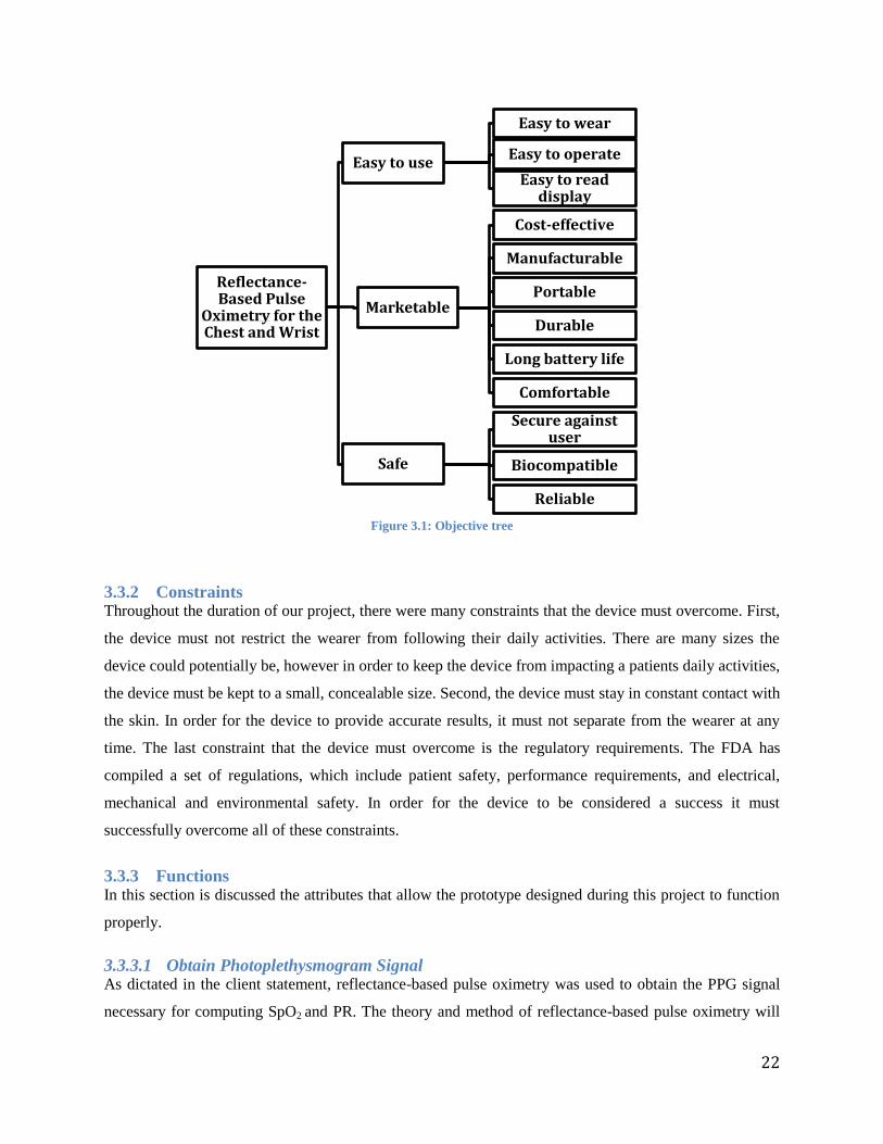
3.3.1 Objectives The objectives consisted of three categories: ‘Easy to use’, ‘Marketable’, and ‘Safe’. ‘Easy to use’

addresses the user friendly nature needed for the device to be useable by the large audience that is to be

targeted. To be easy to use the device must be easy to wear, operate, or read. ‘Marketable’ addresses the

need for the device to be successful and competitive on the market. This means that the device must be

cost-efficient, manufacturable, portable, durable, and comfortable. ‘Safe’ addresses that device must be

safe for the users. Thus the device must be secured against the user to avoid false measurements, be

composed of biocompatible materials as not to cause the user adverse reactions, and conduct reliable

readings.

22

Figure 3.1: Objective tree

3.3.2 Constraints Throughout the duration of our project, there were many constraints that the device must overcome. First,

the device must not restrict the wearer from following their daily activities. There are many sizes the

device could potentially be, however in order to keep the device from impacting a patients daily activities,

the device must be kept to a small, concealable size. Second, the device must stay in constant contact with

the skin. In order for the device to provide accurate results, it must not separate from the wearer at any

time. The last constraint that the device must overcome is the regulatory requirements. The FDA has

compiled a set of regulations, which include patient safety, performance requirements, and electrical,

mechanical and environmental safety. In order for the device to be considered a success it must

successfully overcome all of these constraints.

3.3.3 Functions In this section is discussed the attributes that allow the prototype designed during this project to function

properly.

3.3.3.1 Obtain Photoplethysmogram Signal As dictated in the client statement, reflectance-based pulse oximetry was used to obtain the PPG signal

necessary for computing SpO2 and PR. The theory and method of reflectance-based pulse oximetry will

Reflectance-Based Pulse

Oximetry for the Chest and Wrist

Easy to use

Easy to wear

Easy to operate

Easy to read display

Marketable

Cost-effective

Manufacturable

Portable

Durable

Long battery life

Comfortable

Safe

Secure against user

Biocompatible

Reliable

23

be used to do this from the chest and wrist.

3.3.3.2 Measure Heart Rate In the AC component from the obtained PPG signal, the pulsatile pattern on the top of the PPG signal

reflects the changing blood volume at the site of measurement with each cardiac beat. The signals are

passed through a bandpass filter with a cut-off of about 1.5 Hz, to separate the AC pulses from the DC

signals. The LabVIEW VI developed to process the PPG signal is then used to average the maximum

frequency to determine the rate of the cardiac beat in hertz. This value was then multiplied by 60 to find

the PR in beats per minute.

3.3.3.3 Measure Oxygen Saturation SpO2 is defined as the ratio of HbO2 to the total concentration of Hb present in the blood

[1]. After the

LabVIEW VI processes the PPG signal, it calculates the ratio of red to infrared light used in the

calculation for SpO2.

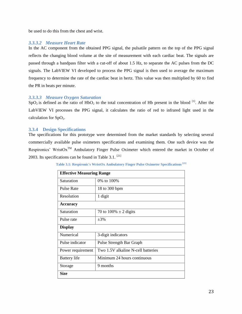
3.3.4 Design Specifications The specifications for this prototype were determined from the market standards by selecting several

commercially available pulse oximeters specifications and examining them. One such device was the

Respironics’ WristOxTM

Ambulatory Finger Pulse Oximeter which entered the market in October of

2003. Its specifications can be found in Table 3.1. [21]

Table 3.1: Respironic's WristOx Ambulatory Finger Pulse Oximeter Specifications [21]

Effective Measuring Range

Saturation 0% to 100%

Pulse Rate 18 to 300 bpm

Resolution 1 digit

Accuracy

Saturation 70 to 100% ± 2 digits

Pulse rate ±3%

Display

Numerical 3-digit indicators

Pulse indicator Pulse Strength Bar Graph

Power requirement Two 1.5V alkaline N-cell batteries

Battery life Minimum 24 hours continuous

Storage 9 months

Size

24

Weight ~0.88 ounces (24.95g)

Dimensions (w/o

sensor or strap)

1.75” wide x 2” high x 0.75” deep

4.45cm x 5.08cm x 1.905cm

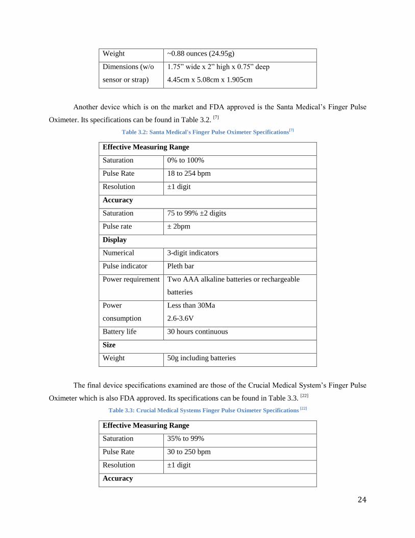
Another device which is on the market and FDA approved is the Santa Medical’s Finger Pulse

Oximeter. Its specifications can be found in Table 3.2. [7]

Table 3.2: Santa Medical's Finger Pulse Oximeter Specifications[7]




Resolution ±1 digit

Accuracy

Saturation 75 to 99% ±2 digits

Pulse rate ± 2bpm

Display


Pulse indicator Pleth bar

Power requirement Two AAA alkaline batteries or rechargeable

batteries

Power

consumption

Less than 30Ma

2.6-3.6V

Battery life 30 hours continuous

Size

Weight 50g including batteries

The final device specifications examined are those of the Crucial Medical System’s Finger Pulse

Oximeter which is also FDA approved. Its specifications can be found in Table 3.3. [22]

Table 3.3: Crucial Medical Systems Finger Pulse Oximeter Specifications [22]




Resolution ±1 digit

Accuracy

25

Saturation 70 to 99% ±2 digits

Pulse rate ± 2bpm

Display


Pulse indicator Bar graph and perfusion index

Power requirement Two AAA alkaline batteries

Power

consumption

Less than 30Ma

2.6-3.6V

Battery life 30 hours continuous

Size

Weight 1.8oz (50g) including batteries

Dimensions 58.5 x31 x32 mm

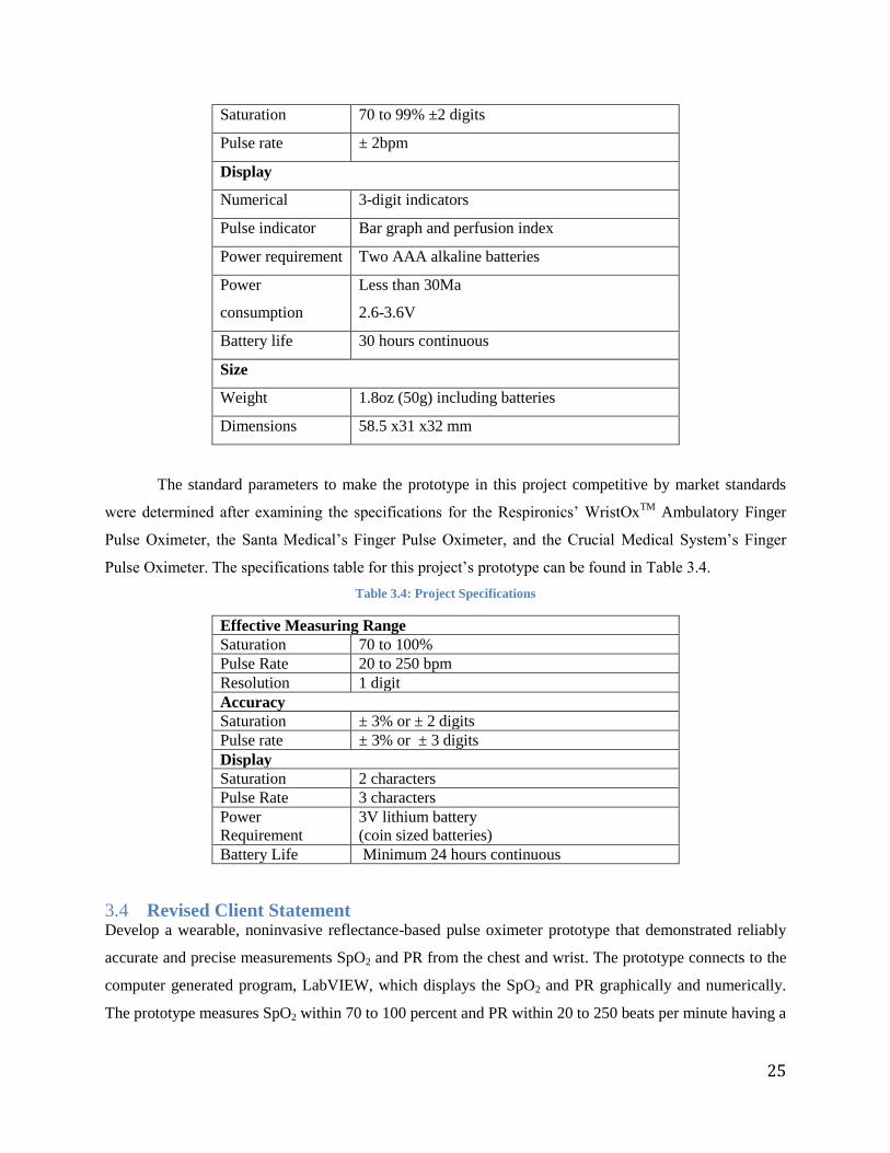
The standard parameters to make the prototype in this project competitive by market standards

were determined after examining the specifications for the Respironics’ WristOxTM

Ambulatory Finger

Pulse Oximeter, the Santa Medical’s Finger Pulse Oximeter, and the Crucial Medical System’s Finger

Pulse Oximeter. The specifications table for this project’s prototype can be found in Table 3.4.

Table 3.4: Project Specifications


Saturation 70 to 100%


Resolution 1 digit

Accuracy

Saturation ± 3% or ± 2 digits

Pulse rate ± 3% or ± 3 digits

Display

Saturation 2 characters

Pulse Rate 3 characters

Power

Requirement

3V lithium battery

(coin sized batteries)

Battery Life Minimum 24 hours continuous

Revised Client Statement 3.4Develop a wearable, noninvasive reflectance-based pulse oximeter prototype that demonstrated reliably

accurate and precise measurements SpO2 and PR from the chest and wrist. The prototype connects to the

computer generated program, LabVIEW, which displays the SpO2 and PR graphically and numerically.

The prototype measures SpO2 within 70 to 100 percent and PR within 20 to 250 beats per minute having a

26

resolution of 1 digit and accuracy within ±3% or ±3 digits. This prototype should weigh less than 150

grams. The prototype must not cause any harm, such as burning the skin or allergic reactions. In order to

provide the best results possible for SpO2 and PR, the prototype must remain in constant contact with the

skin. This prototype should be easy to use, requiring little to no training before use. Once the prototype is

completed, testing for this device was conducted on healthy volunteers to test the accuracy and precision

as well as proving that SpO2 and PR can be measured from the chest and wrist.

27

4 Device Development

Device Alternatives 4.1

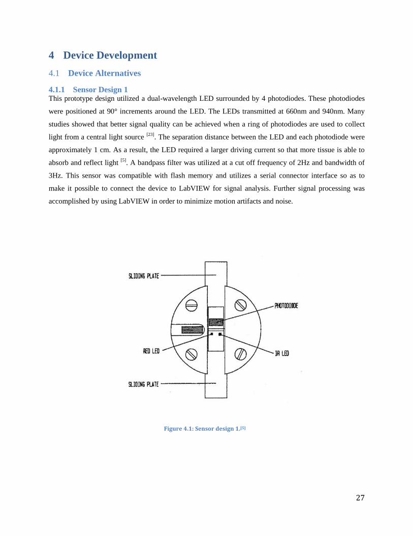
4.1.1 Sensor Design 1 This prototype design utilized a dual-wavelength LED surrounded by 4 photodiodes. These photodiodes

were positioned at 90° increments around the LED. The LEDs transmitted at 660nm and 940nm. Many

studies showed that better signal quality can be achieved when a ring of photodiodes are used to collect

light from a central light source [23]

. The separation distance between the LED and each photodiode were

approximately 1 cm. As a result, the LED required a larger driving current so that more tissue is able to

absorb and reflect light [5]

. A bandpass filter was utilized at a cut off frequency of 2Hz and bandwidth of

3Hz. This sensor was compatible with flash memory and utilizes a serial connector interface so as to

make it possible to connect the device to LabVIEW for signal analysis. Further signal processing was

accomplished by using LabVIEW in order to minimize motion artifacts and noise.

Figure 4.1: Sensor design 1.[5]

28

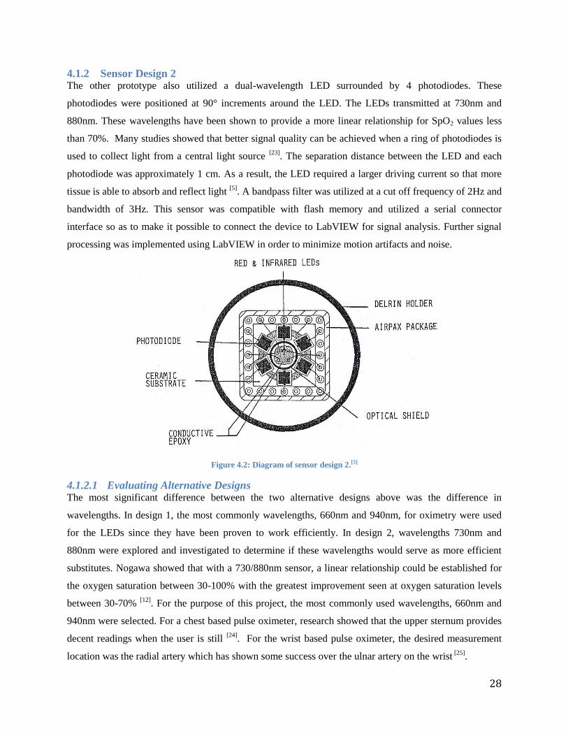
4.1.2 Sensor Design 2 The other prototype also utilized a dual-wavelength LED surrounded by 4 photodiodes. These

photodiodes were positioned at 90° increments around the LED. The LEDs transmitted at 730nm and

880nm. These wavelengths have been shown to provide a more linear relationship for SpO2 values less

than 70%. Many studies showed that better signal quality can be achieved when a ring of photodiodes is

used to collect light from a central light source [23]

. The separation distance between the LED and each

photodiode was approximately 1 cm. As a result, the LED required a larger driving current so that more

tissue is able to absorb and reflect light [5]

. A bandpass filter was utilized at a cut off frequency of 2Hz and

bandwidth of 3Hz. This sensor was compatible with flash memory and utilized a serial connector

interface so as to make it possible to connect the device to LabVIEW for signal analysis. Further signal

processing was implemented using LabVIEW in order to minimize motion artifacts and noise.

Figure 4.2: Diagram of sensor design 2.[5]

4.1.2.1 Evaluating Alternative Designs The most significant difference between the two alternative designs above was the difference in

wavelengths. In design 1, the most commonly wavelengths, 660nm and 940nm, for oximetry were used

for the LEDs since they have been proven to work efficiently. In design 2, wavelengths 730nm and

880nm were explored and investigated to determine if these wavelengths would serve as more efficient

substitutes. Nogawa showed that with a 730/880nm sensor, a linear relationship could be established for

the oxygen saturation between 30-100% with the greatest improvement seen at oxygen saturation levels

between 30-70% [12]

. For the purpose of this project, the most commonly used wavelengths, 660nm and

940nm were selected. For a chest based pulse oximeter, research showed that the upper sternum provides

decent readings when the user is still [24]

. For the wrist based pulse oximeter, the desired measurement

location was the radial artery which has shown some success over the ulnar artery on the wrist [25]

.

29

Software Design 4.2

The program used to compute SpO2 and PR from the PPG signals gathered by the sensor is LabVIEW

System Design Software from National Instruments. Each program created within LabVIEW is known as

a virtual instrument (VI).

30

5 Methods

Photodetection Unit 5.1The photodetection unit used in this project utilizes LEDs and photodiodes to collect backscattered light

that travels from the LED, through skin and tissue and is reflected off the bones and subcutaneous tissues

back into the photodiode. Our ability to measure the PPG and calculate SpO2 comes from the varying

absorption that occurs as the heart pumps blood through the arteries. For the photodetection unit to

properly work, the LED and photodiode must be close enough to each other so the photodiode can pick

up the greatest fraction of backscattered light for the highest possible output and signal to noise ratio.

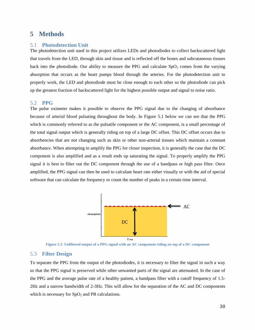
PPG 5.2The pulse oximeter makes it possible to observe the PPG signal due to the changing of absorbance

because of arterial blood pulsating throughout the body. In Figure 5.1 below we can see that the PPG

which is commonly referred to as the pulsatile component or the AC component, is a small percentage of

the total signal output which is generally riding on top of a large DC offset. This DC offset occurs due to

absorbencies that are not changing such as skin or other non-arterial tissues which maintain a constant

absorbance. When attempting to amplify the PPG for closer inspection, it is generally the case that the DC

component is also amplified and as a result ends up saturating the signal. To properly amplify the PPG

signal it is best to filter out the DC component through the use of a bandpass or high pass filter. Once

amplified, the PPG signal can then be used to calculate heart rate either visually or with the aid of special

software that can calculate the frequency or count the number of peaks in a certain time interval.

Figure 5.1: Unfiltered output of a PPG signal with an AC component riding on top of a DC component

Filter Design 5.3

To separate the PPG from the output of the photodiodes, it is necessary to filter the signal in such a way

so that the PPG signal is preserved while other unwanted parts of the signal are attenuated. In the case of

the PPG and the average pulse rate of a healthy patient, a bandpass filter with a cutoff frequency of 1.5-

2Hz and a narrow bandwidth of 2-3Hz. This will allow for the separation of the AC and DC components

which is necessary for SpO2 and PR calculations.

DC

AC

31

Software 5.4

Signals were digitized and sampled using LabVIEW DAQ Assistant with analog inputs collected by a

National Instrument’s Data Acquisition Board with a sampling frequency of 100Hz. The functions of the

software are described in Appendix A and can provide further detail into the design of the VI used for this

prototype.

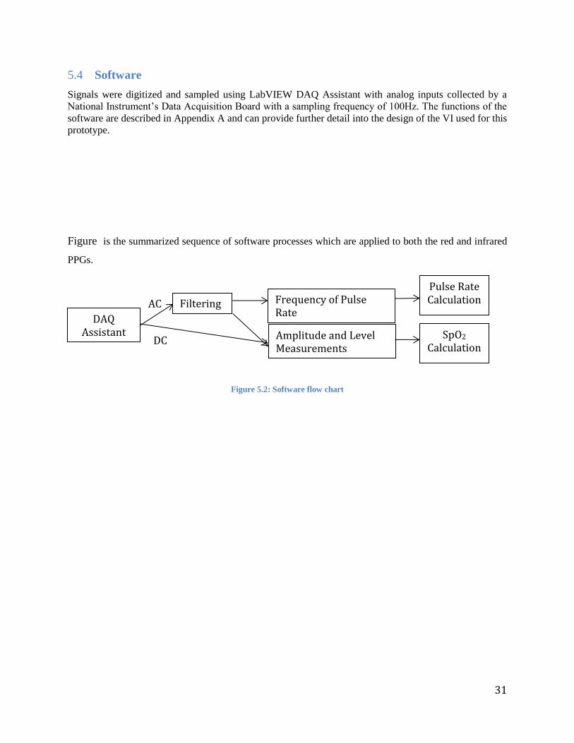
Figure is the summarized sequence of software processes which are applied to both the red and infrared

PPGs.

Figure 5.2: Software flow chart

DC

AC

DAQ Assistant

Filtering Frequency of Pulse Rate

Amplitude and Level Measurements

Pulse Rate Calculation

SpO2 Calculation

32

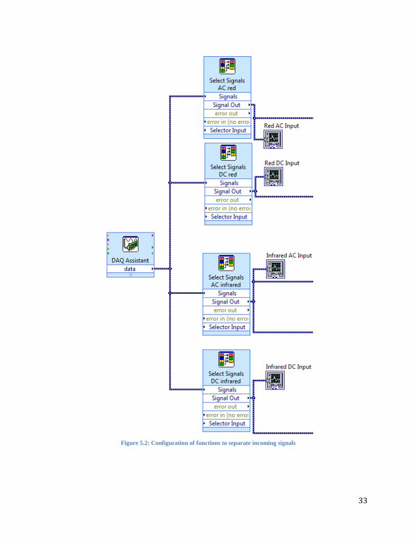
5.4.1 Incoming Signals

The first block in the Software Flow Chart, in Figure 5.2 is to address the installation of the external DAQ

Assistant and the completion of its internal task which includes identifying the connected external DAQ

Assistant with the DAQ Assistant function in the Block Diagram, each of the incoming signal channels,

and the sampling rate. Since the DAQ Assistant function combines the four incoming signals created by

the sensor into a single output called data, four Select Signals functions are used to separate and identify

the incoming signals. The Select Signal functions were used instead of a simple Split Signal function

because they could be set to single out a one specific signal while a Split Signal would separate the

signals, but provide no indication of which signal was being produced. To ensure that the DAQ Assistant

external and internal system was receiving the signals correctly, Waveform Graphs were implemented at

the output of each Select Signals which when the prototype was running would plot the AC and DC

components of the red and infrared signals and be compared to the readings of an oscilloscope.

33

Figure 5.2: Configuration of functions to separate incoming signals

34

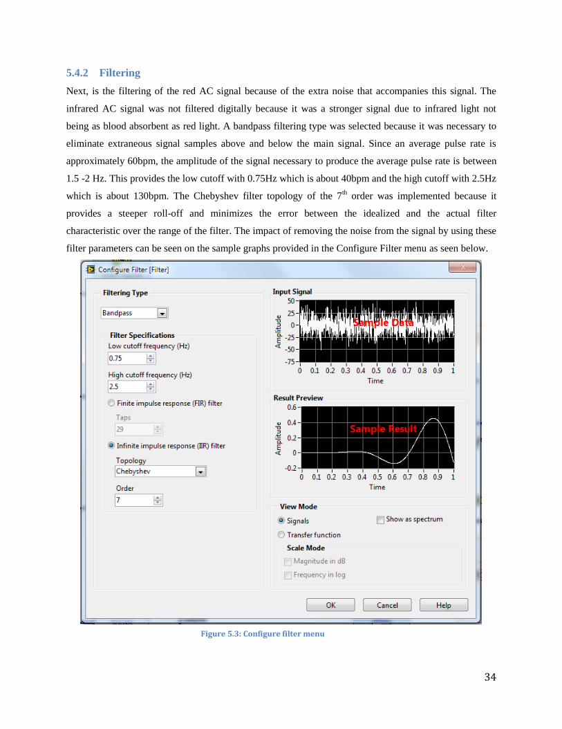
5.4.2 Filtering

Next, is the filtering of the red AC signal because of the extra noise that accompanies this signal. The

infrared AC signal was not filtered digitally because it was a stronger signal due to infrared light not

being as blood absorbent as red light. A bandpass filtering type was selected because it was necessary to

eliminate extraneous signal samples above and below the main signal. Since an average pulse rate is

approximately 60bpm, the amplitude of the signal necessary to produce the average pulse rate is between

1.5 -2 Hz. This provides the low cutoff with 0.75Hz which is about 40bpm and the high cutoff with 2.5Hz

which is about 130bpm. The Chebyshev filter topology of the 7th order was implemented because it

provides a steeper roll-off and minimizes the error between the idealized and the actual filter

characteristic over the range of the filter. The impact of removing the noise from the signal by using these

filter parameters can be seen on the sample graphs provided in the Configure Filter menu as seen below.

Figure 5.3: Configure filter menu

35

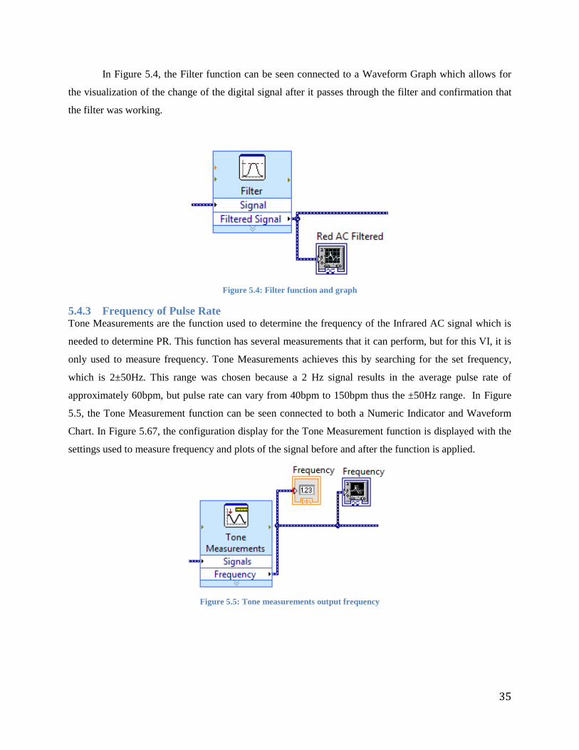
In Figure 5.4, the Filter function can be seen connected to a Waveform Graph which allows for

the visualization of the change of the digital signal after it passes through the filter and confirmation that

the filter was working.

Figure 5.4: Filter function and graph

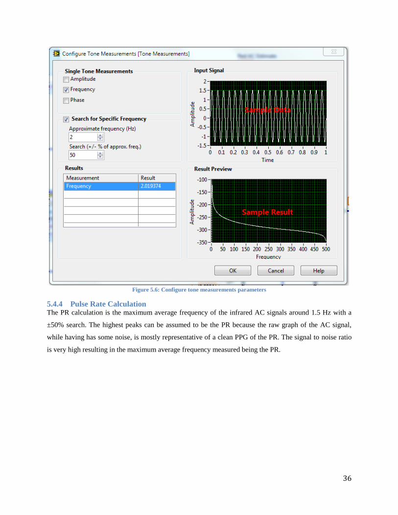
5.4.3 Frequency of Pulse Rate Tone Measurements are the function used to determine the frequency of the Infrared AC signal which is

needed to determine PR. This function has several measurements that it can perform, but for this VI, it is

only used to measure frequency. Tone Measurements achieves this by searching for the set frequency,

which is 2±50Hz. This range was chosen because a 2 Hz signal results in the average pulse rate of

approximately 60bpm, but pulse rate can vary from 40bpm to 150bpm thus the ±50Hz range. In Figure

5.5, the Tone Measurement function can be seen connected to both a Numeric Indicator and Waveform

Chart. In Figure 5.67, the configuration display for the Tone Measurement function is displayed with the

settings used to measure frequency and plots of the signal before and after the function is applied.

Figure 5.5: Tone measurements output frequency

36

Figure 5.6: Configure tone measurements parameters

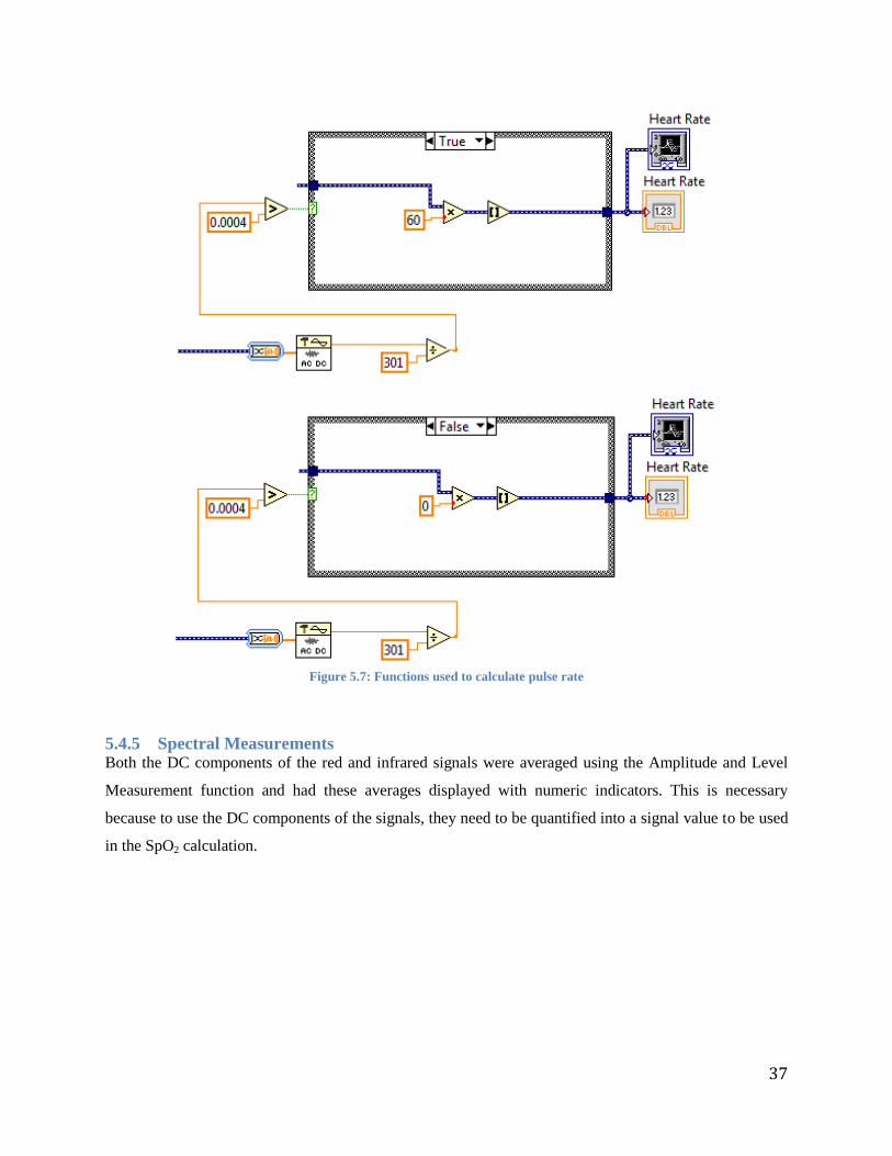
5.4.4 Pulse Rate Calculation The PR calculation is the maximum average frequency of the infrared AC signals around 1.5 Hz with a

±50% search. The highest peaks can be assumed to be the PR because the raw graph of the AC signal,

while having has some noise, is mostly representative of a clean PPG of the PR. The signal to noise ratio

is very high resulting in the maximum average frequency measured being the PR.

37

Figure 5.7: Functions used to calculate pulse rate

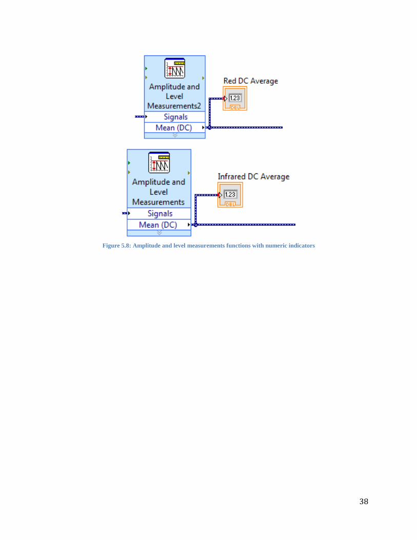
5.4.5 Spectral Measurements Both the DC components of the red and infrared signals were averaged using the Amplitude and Level

Measurement function and had these averages displayed with numeric indicators. This is necessary

because to use the DC components of the signals, they need to be quantified into a signal value to be used

in the SpO2 calculation.

38

Figure 5.8: Amplitude and level measurements functions with numeric indicators

39

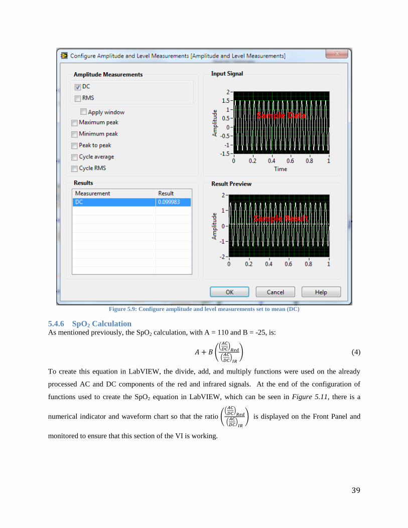
Figure 5.9: Configure amplitude and level measurements set to mean (DC)

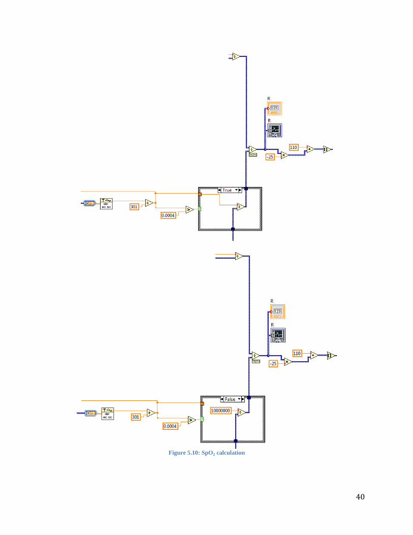
5.4.6 SpO2 Calculation As mentioned previously, the SpO2 calculation, with A = 110 and B = -25, is:

((

)

(

)

) (4)

To create this equation in LabVIEW, the divide, add, and multiply functions were used on the already

processed AC and DC components of the red and infrared signals. At the end of the configuration of

functions used to create the SpO2 equation in LabVIEW, which can be seen in Figure 5.11, there is a

numerical indicator and waveform chart so that the ratio ((

)

(

)

) is displayed on the Front Panel and

monitored to ensure that this section of the VI is working.

40

Figure 5.10: SpO2 calculation

41

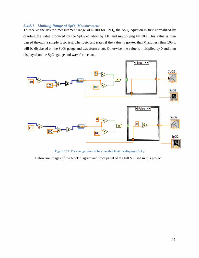
5.4.6.1 Limiting Range of SpO2 Measurement To receive the desired measurement range of 0-100 for SpO2, the SpO2 equation is first normalized by

dividing the value produced by the SpO2 equation by 110 and multiplying by 100. This value is then

passed through a simple logic test. The logic test states if the value is greater than 0 and less than 100 it

will be displayed on the SpO2 gauge and waveform chart. Otherwise, the value is multiplied by 0 and then

displayed on the SpO2 gauge and waveform chart.

Figure 5.11: The configuration of function that limit the displayed SpO2

Below are images of the block diagram and front panel of the full VI used in this project.

42

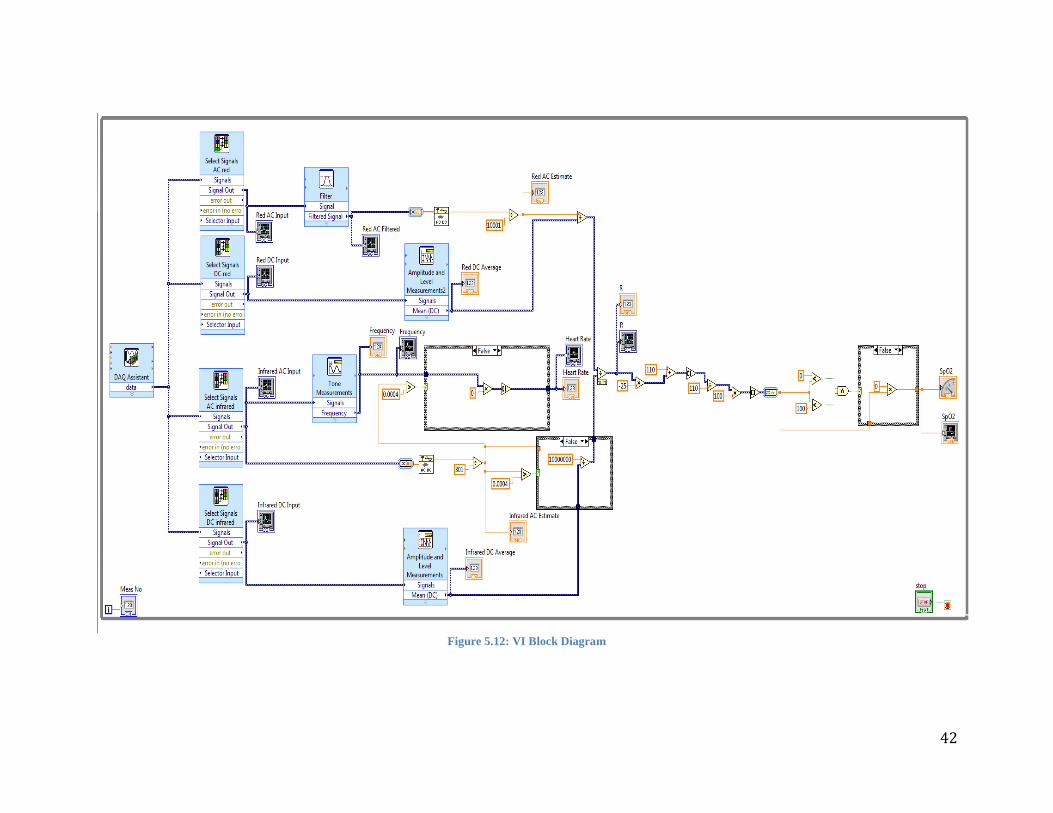
Figure 5.12: VI Block Diagram

43

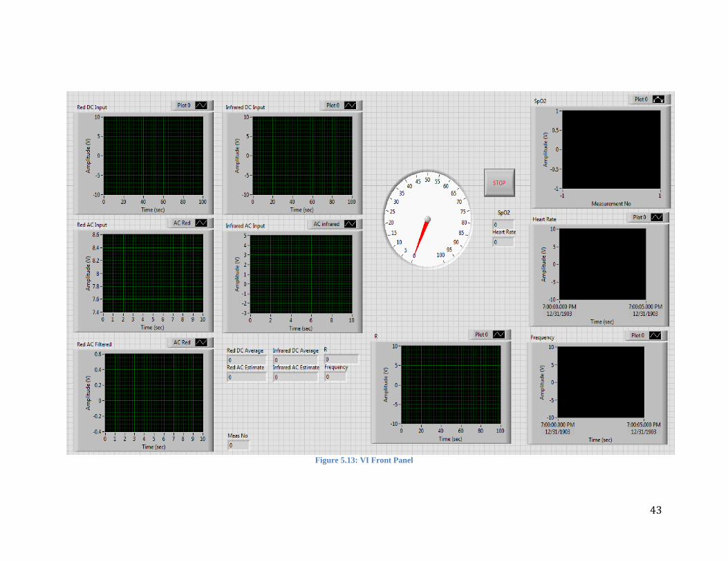
Figure 5.13: VI Front Panel

44

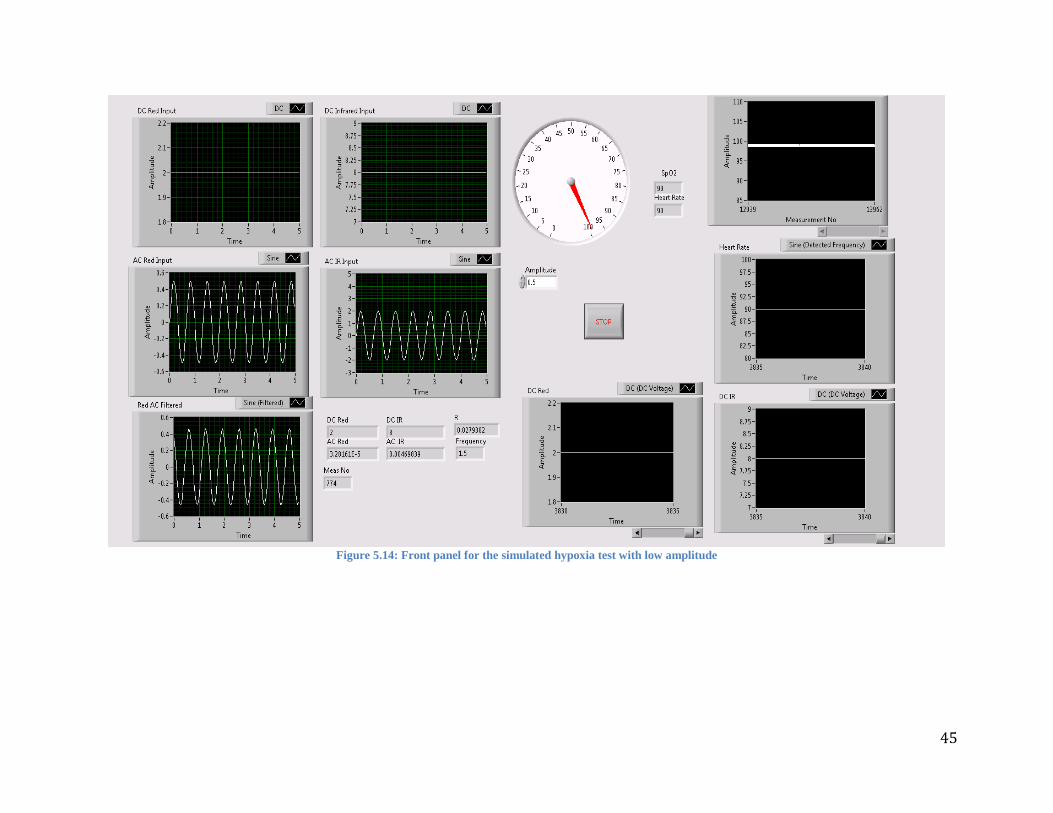
5.4.7 Preliminary VI Test To test the VI, four digitally simulated signals were used with a control, a function in LabVIEW that will

allow the manipulation of a variable while the VI is running, was placed on the amplitude of the red AC

signal. This control was used to manually increase the red AC signal’s amplitude causing the SpO2 to

decrease. This test of the VI replicated the oxygen decrease in the blood of a person who was hypoxic.

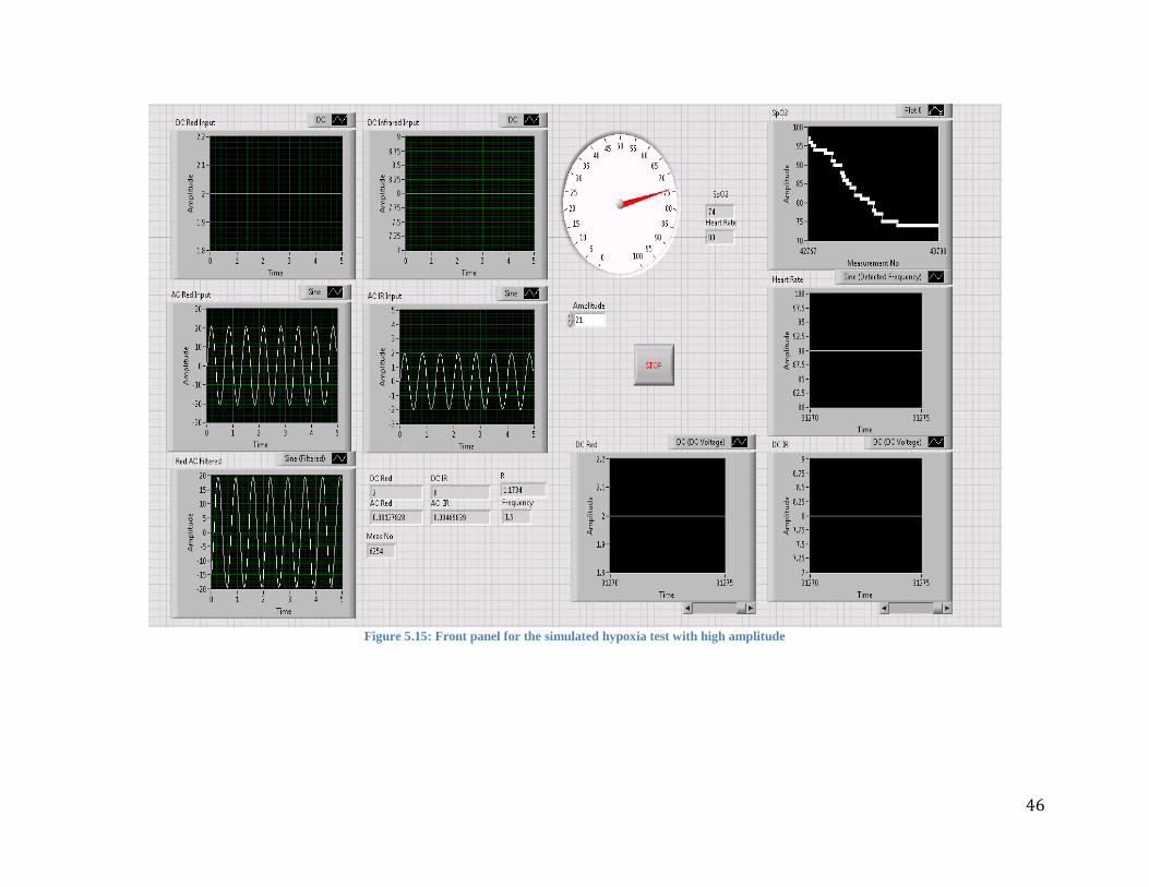
Below are images that demonstrate the success of this preliminary test of the VI. Figure 5.15,

depicts the VI at the start of the test with the amplitude control at 0.5, the control can be seen below the

SpO2 gage and to the left of the LabVIEW stop button. Since the amplitude control has not been changed

yet the SpO2 graph in the upper right of the figure is a straight line and the AC Red Input and Red AC

Filtered graphs have the relatively large amplitudes of 20Hz. As the amplitude control is slowly increased

to 21, the SpO2 graph in the upper right of Figure 5.16 shows a steady decrease and the AC Red Input and

Red AC Filtered graphs now have amplitudes of 0.4Hz.

The “R” indicator, which displays the ratio value calculated during the SpO2 calculation, is seen

to increase between the two figures, as it was expected, because it is necessary for the ratio to increase for

the resulting SpO2 to decrease. The other graphs and indicators do not show a change in between Figure

5.15 and 5.16 because this was a controlled tested with simulated input signals.

45

Figure 5.14: Front panel for the simulated hypoxia test with low amplitude

46

Figure 5.15: Front panel for the simulated hypoxia test with high amplitude

47

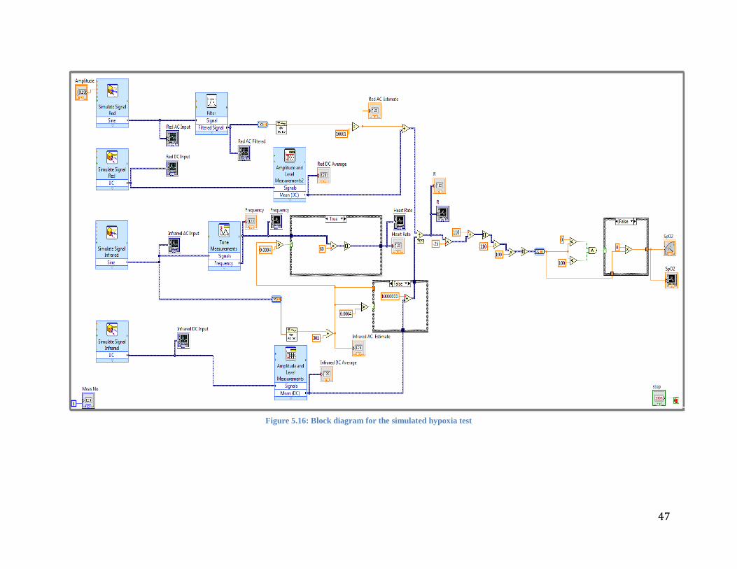
Figure 5.16: Block diagram for the simulated hypoxia test

48

Experimentation/Testing 5.5

5.5.1.1 ECG and Reference Pulse Oximeter Reliability Test For measurement and comparison purposes a HOMEDICS Deluxe Pulse Oximeter with transmission

method for the finger was utilized as a reference along with our pulse oximeter prototype. The reliability

of the reference pulse oximeter was tested against an ECG Biopac module model 100C.

Three ECG electrodes were connected to each subject’s right arm, left arm and left leg. Data

collected from the ECG electrodes were displayed by the AcqKnowledge software and changes in PR

were monitored on the screen using peak to peak analysis. The pulse oximeter was placed on the subject’s

index finger. The ECG Biopac module was turned on and one minute of data were collected while the PR

was monitored by the finger pulse oximeter at the same time. Accuracy and error percentages were

calculated from each measurement. We calculated the error to be less than +3%, which matches the finger

pulse oximeter’s specification sheet and deems it suitable to use as a reference.

5.5.1.2 Wrist Measurements The probe of an oscilloscope was connected to the AC infrared outlet of the circuit and to common

ground. The display of the oscilloscope was set up to segments of 500 milliseconds with amplitude of 2

volts so the blood pressure wave was clearly visualized. Since the AC component of the infrared outlet

from the circuit showed a more defined representation of the blood pressure curve than the AC red

component, the AC infrared component was utilized as a second visual reference for the testing phase of

the prototype.

The sensor was strapped tightly to the wrist of the subject by means of a Velcro strap to maintain

constant pressure while the subject was sitting with his/her arm resting on a table. Although we

encouraged the subjects to place the sensor directly over the radial artery, the specific location and

orientation of the sensor varied for each individual since PPG intensity can vary from person to person.

49

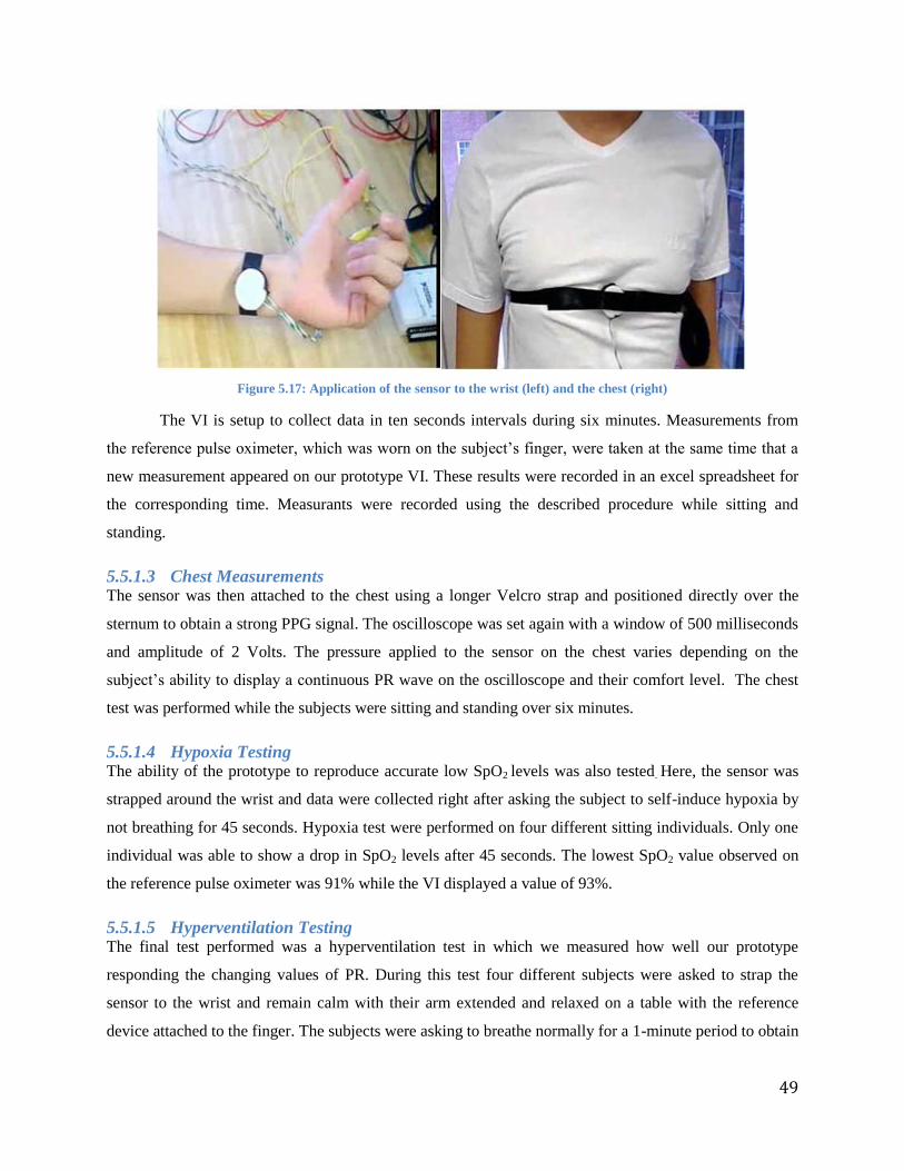
Figure 5.17: Application of the sensor to the wrist (left) and the chest (right)

The VI is setup to collect data in ten seconds intervals during six minutes. Measurements from

the reference pulse oximeter, which was worn on the subject’s finger, were taken at the same time that a

new measurement appeared on our prototype VI. These results were recorded in an excel spreadsheet for

the corresponding time. Measurants were recorded using the described procedure while sitting and

standing.

5.5.1.3 Chest Measurements The sensor was then attached to the chest using a longer Velcro strap and positioned directly over the

sternum to obtain a strong PPG signal. The oscilloscope was set again with a window of 500 milliseconds

and amplitude of 2 Volts. The pressure applied to the sensor on the chest varies depending on the

subject’s ability to display a continuous PR wave on the oscilloscope and their comfort level. The chest

test was performed while the subjects were sitting and standing over six minutes.

5.5.1.4 Hypoxia Testing The ability of the prototype to reproduce accurate low SpO2 levels was also tested. Here, the sensor was

strapped around the wrist and data were collected right after asking the subject to self-induce hypoxia by

not breathing for 45 seconds. Hypoxia test were performed on four different sitting individuals. Only one

individual was able to show a drop in SpO2 levels after 45 seconds. The lowest SpO2 value observed on

the reference pulse oximeter was 91% while the VI displayed a value of 93%.

5.5.1.5 Hyperventilation Testing The final test performed was a hyperventilation test in which we measured how well our prototype

responding the changing values of PR. During this test four different subjects were asked to strap the

sensor to the wrist and remain calm with their arm extended and relaxed on a table with the reference

device attached to the finger. The subjects were asking to breathe normally for a 1-minute period to obtain

50

a stable PR. After the initial minute, each subject was then asked to begin hyperventilating for about 4

minutes. After the hyperventilation period the subjects were asked to breathe normally again for an

additional minute to conclude the 6 min test and to show a declining PR. The results were compared to

the reference device and plotted data were produced and shown in the results section.

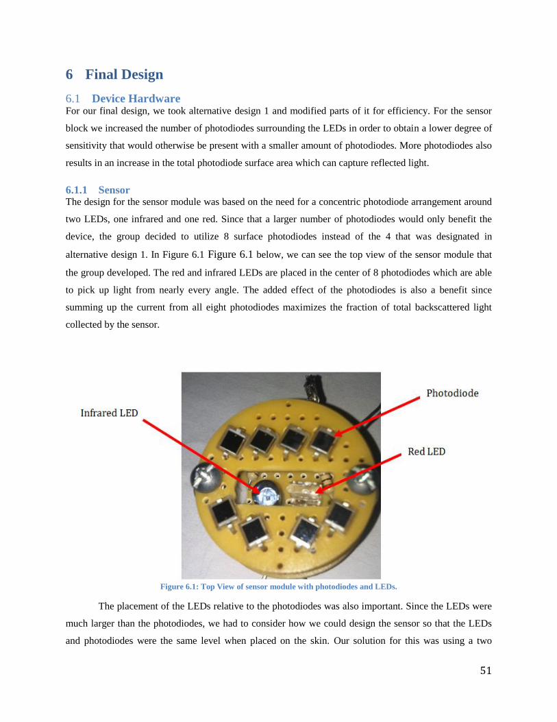
51

6 Final Design

Device Hardware 6.1For our final design, we took alternative design 1 and modified parts of it for efficiency. For the sensor

block we increased the number of photodiodes surrounding the LEDs in order to obtain a lower degree of

sensitivity that would otherwise be present with a smaller amount of photodiodes. More photodiodes also

results in an increase in the total photodiode surface area which can capture reflected light.

6.1.1 Sensor The design for the sensor module was based on the need for a concentric photodiode arrangement around

two LEDs, one infrared and one red. Since that a larger number of photodiodes would only benefit the

device, the group decided to utilize 8 surface photodiodes instead of the 4 that was designated in

alternative design 1. In Figure 6.1 Figure 6.1 below, we can see the top view of the sensor module that

the group developed. The red and infrared LEDs are placed in the center of 8 photodiodes which are able

to pick up light from nearly every angle. The added effect of the photodiodes is also a benefit since

summing up the current from all eight photodiodes maximizes the fraction of total backscattered light

collected by the sensor.

Figure 6.1: Top View of sensor module with photodiodes and LEDs.

The placement of the LEDs relative to the photodiodes was also important. Since the LEDs were

much larger than the photodiodes, we had to consider how we could design the sensor so that the LEDs

and photodiodes were the same level when placed on the skin. Our solution for this was using a two

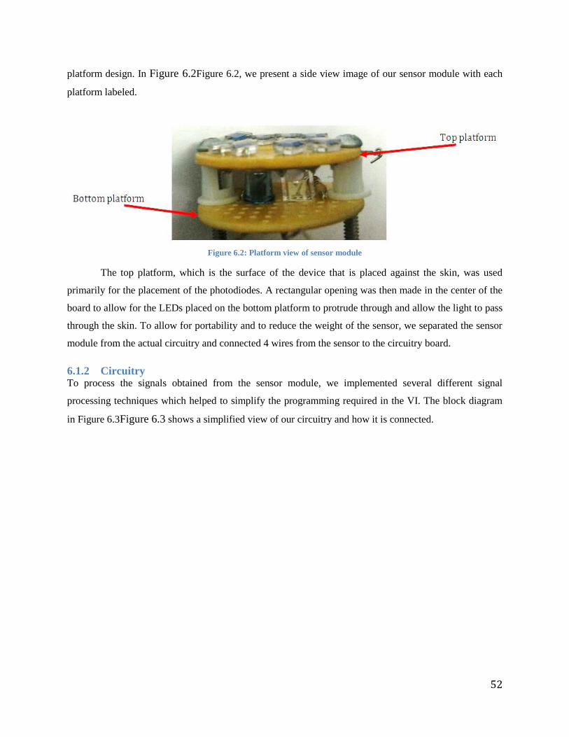
52

platform design. In Figure 6.2Figure 6.2, we present a side view image of our sensor module with each

platform labeled.

Figure 6.2: Platform view of sensor module

The top platform, which is the surface of the device that is placed against the skin, was used

primarily for the placement of the photodiodes. A rectangular opening was then made in the center of the

board to allow for the LEDs placed on the bottom platform to protrude through and allow the light to pass

through the skin. To allow for portability and to reduce the weight of the sensor, we separated the sensor

module from the actual circuitry and connected 4 wires from the sensor to the circuitry board.

6.1.2 Circuitry To process the signals obtained from the sensor module, we implemented several different signal

processing techniques which helped to simplify the programming required in the VI. The block diagram

in Figure 6.3Figure 6.3 shows a simplified view of our circuitry and how it is connected.

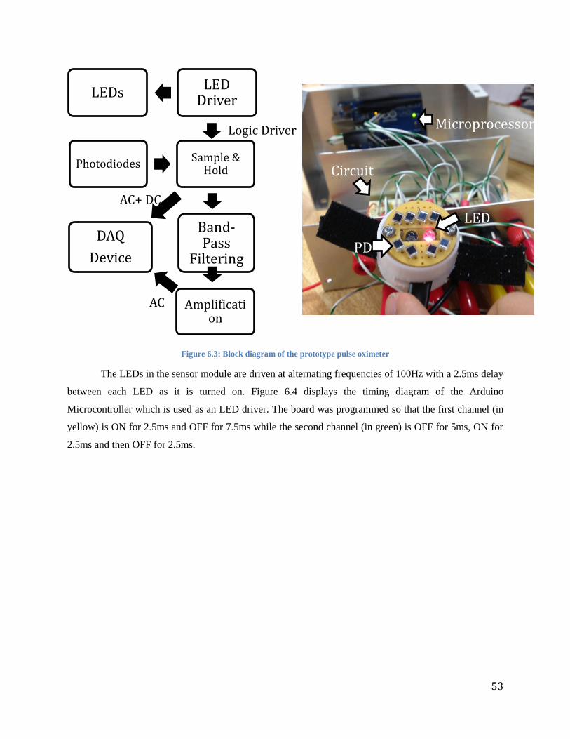
53

Figure 6.3: Block diagram of the prototype pulse oximeter

The LEDs in the sensor module are driven at alternating frequencies of 100Hz with a 2.5ms delay

between each LED as it is turned on. Figure 6.4 displays the timing diagram of the Arduino

Microcontroller which is used as an LED driver. The board was programmed so that the first channel (in

yellow) is ON for 2.5ms and OFF for 7.5ms while the second channel (in green) is OFF for 5ms, ON for

2.5ms and then OFF for 2.5ms.

AC+ DC

Logic Driver

AC

LEDs LED

Driver

Photodiodes Sample &

Hold

DAQ

Device

Band-Pass

Filtering

Amplification

PD

LED

Microprocessor

Circuit

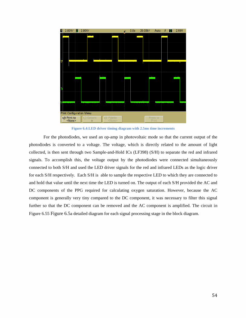
54

Figure 6.4:LED driver timing diagram with 2.5ms time increments

For the photodiodes, we used an op-amp in photovoltaic mode so that the current output of the

photodiodes is converted to a voltage. The voltage, which is directly related to the amount of light

collected, is then sent through two Sample-and-Hold ICs (LF398) (S/H) to separate the red and infrared

signals. To accomplish this, the voltage output by the photodiodes were connected simultaneously

connected to both S/H and used the LED driver signals for the red and infrared LEDs as the logic driver

for each S/H respectively. Each S/H is able to sample the respective LED to which they are connected to

and hold that value until the next time the LED is turned on. The output of each S/H provided the AC and

DC components of the PPG required for calculating oxygen saturation. However, because the AC

component is generally very tiny compared to the DC component, it was necessary to filter this signal

further so that the DC component can be removed and the AC component is amplified. The circuit in

Figure 6.55 Figure 6.5a detailed diagram for each signal processing stage in the block diagram.

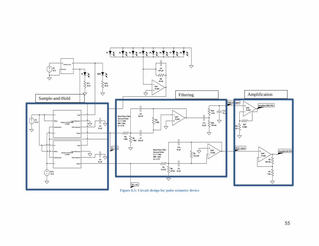
55

Figure 6.5: Circuit design for pulse oximeter device

Sample-and-Hold Filtering Amplification

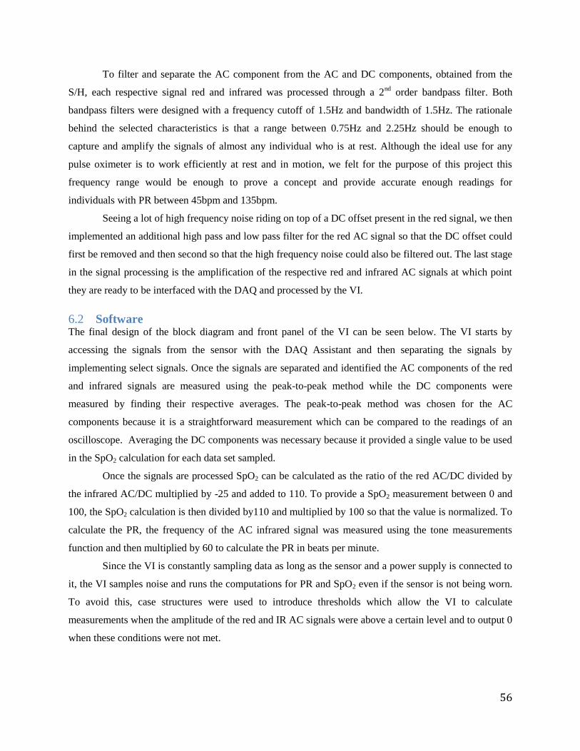
56

To filter and separate the AC component from the AC and DC components, obtained from the

S/H, each respective signal red and infrared was processed through a 2nd

order bandpass filter. Both

bandpass filters were designed with a frequency cutoff of 1.5Hz and bandwidth of 1.5Hz. The rationale

behind the selected characteristics is that a range between 0.75Hz and 2.25Hz should be enough to

capture and amplify the signals of almost any individual who is at rest. Although the ideal use for any

pulse oximeter is to work efficiently at rest and in motion, we felt for the purpose of this project this

frequency range would be enough to prove a concept and provide accurate enough readings for

individuals with PR between 45bpm and 135bpm.

Seeing a lot of high frequency noise riding on top of a DC offset present in the red signal, we then

implemented an additional high pass and low pass filter for the red AC signal so that the DC offset could

first be removed and then second so that the high frequency noise could also be filtered out. The last stage

in the signal processing is the amplification of the respective red and infrared AC signals at which point

they are ready to be interfaced with the DAQ and processed by the VI.

Software 6.2The final design of the block diagram and front panel of the VI can be seen below. The VI starts by

accessing the signals from the sensor with the DAQ Assistant and then separating the signals by

implementing select signals. Once the signals are separated and identified the AC components of the red

and infrared signals are measured using the peak-to-peak method while the DC components were

measured by finding their respective averages. The peak-to-peak method was chosen for the AC

components because it is a straightforward measurement which can be compared to the readings of an

oscilloscope. Averaging the DC components was necessary because it provided a single value to be used

in the SpO2 calculation for each data set sampled.

Once the signals are processed SpO2 can be calculated as the ratio of the red AC/DC divided by

the infrared AC/DC multiplied by -25 and added to 110. To provide a SpO2 measurement between 0 and

100, the SpO2 calculation is then divided by110 and multiplied by 100 so that the value is normalized. To

calculate the PR, the frequency of the AC infrared signal was measured using the tone measurements

function and then multiplied by 60 to calculate the PR in beats per minute.

Since the VI is constantly sampling data as long as the sensor and a power supply is connected to

it, the VI samples noise and runs the computations for PR and SpO2 even if the sensor is not being worn.

To avoid this, case structures were used to introduce thresholds which allow the VI to calculate

measurements when the amplitude of the red and IR AC signals were above a certain level and to output 0

when these conditions were not met.

57

Figure 6.6: Block Diagram of Final VI

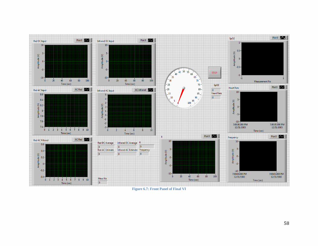
58

Figure 6.7: Front Panel of Final VI

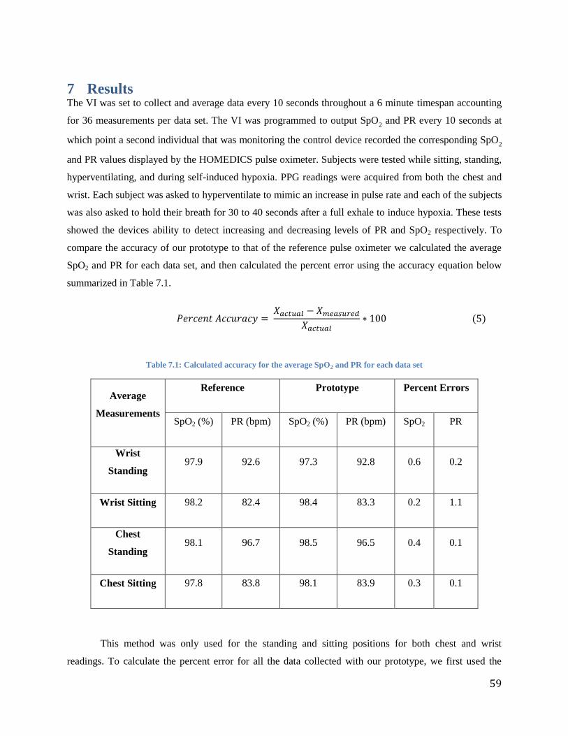
59

7 Results The VI was set to collect and average data every 10 seconds throughout a 6 minute timespan accounting

for 36 measurements per data set. The VI was programmed to output SpO2 and PR every 10 seconds at

which point a second individual that was monitoring the control device recorded the corresponding SpO2

and PR values displayed by the HOMEDICS pulse oximeter. Subjects were tested while sitting, standing,

hyperventilating, and during self-induced hypoxia. PPG readings were acquired from both the chest and

wrist. Each subject was asked to hyperventilate to mimic an increase in pulse rate and each of the subjects

was also asked to hold their breath for 30 to 40 seconds after a full exhale to induce hypoxia. These tests

showed the devices ability to detect increasing and decreasing levels of PR and SpO2 respectively. To

compare the accuracy of our prototype to that of the reference pulse oximeter we calculated the average

SpO2 and PR for each data set, and then calculated the percent error using the accuracy equation below

summarized in Table 7.1.

( )

Table 7.1: Calculated accuracy for the average SpO2 and PR for each data set

Average

Measurements

Reference Prototype Percent Errors

SpO2 (%) PR (bpm) SpO2 (%) PR (bpm) SpO2 PR

Wrist

Standing 97.9 92.6 97.3 92.8 0.6 0.2

Wrist Sitting 98.2 82.4 98.4 83.3 0.2 1.1

Chest

Standing 98.1 96.7 98.5 96.5 0.4 0.1

Chest Sitting 97.8 83.8 98.1 83.9 0.3 0.1

This method was only used for the standing and sitting positions for both chest and wrist

readings. To calculate the percent error for all the data collected with our prototype, we first used the

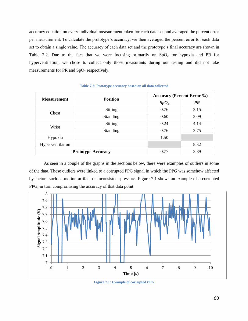
60

accuracy equation on every individual measurement taken for each data set and averaged the percent error

per measurement. To calculate the prototype’s accuracy, we then averaged the percent error for each data

set to obtain a single value. The accuracy of each data set and the prototype’s final accuracy are shown in

Table 7.2. Due to the fact that we were focusing primarily on SpO2 for hypoxia and PR for

hyperventilation, we chose to collect only those measurants during our testing and did not take

measurements for PR and SpO2 respectively.

Table 7.2: Prototype accuracy based on all data collected

Measurement Position Accuracy (Percent Error %)

SpO2 PR

Chest Sitting 0.76 3.15

Standing 0.60 3.09

Wrist Sitting 0.24 4.14

Standing 0.76 3.75

Hypoxia

1.50

Hyperventilation

5.32

Prototype Accuracy 0.77 3.89

As seen in a couple of the graphs in the sections below, there were examples of outliers in some

of the data. These outliers were linked to a corrupted PPG signal in which the PPG was somehow affected

by factors such as motion artifact or inconsistent pressure. Figure 7.1 shows an example of a corrupted

PPG, in turn compromising the accuracy of that data point.

Figure 7.1: Example of corrupted PPG

7

7.1

7.2

7.3

7.4

7.5

7.6

7.7

7.8

7.9

8

0 1 2 3 4 5 6 7 8 9 10

Sig

na

l A

mp

litu

de

(V

)

Time (s)

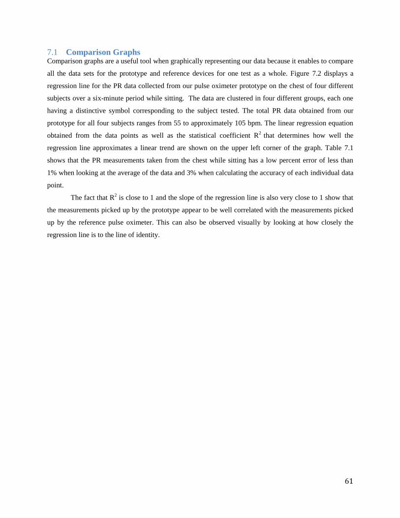
61

Comparison Graphs 7.1Comparison graphs are a useful tool when graphically representing our data because it enables to compare

all the data sets for the prototype and reference devices for one test as a whole. Figure 7.2 displays a

regression line for the PR data collected from our pulse oximeter prototype on the chest of four different

subjects over a six-minute period while sitting. The data are clustered in four different groups, each one

having a distinctive symbol corresponding to the subject tested. The total PR data obtained from our

prototype for all four subjects ranges from 55 to approximately 105 bpm. The linear regression equation

obtained from the data points as well as the statistical coefficient R2

that determines how well the

regression line approximates a linear trend are shown on the upper left corner of the graph. Table 7.1

shows that the PR measurements taken from the chest while sitting has a low percent error of less than

1% when looking at the average of the data and 3% when calculating the accuracy of each individual data

point.

The fact that R2 is close to 1 and the slope of the regression line is also very close to 1 show that

the measurements picked up by the prototype appear to be well correlated with the measurements picked

up by the reference pulse oximeter. This can also be observed visually by looking at how closely the

regression line is to the line of identity.

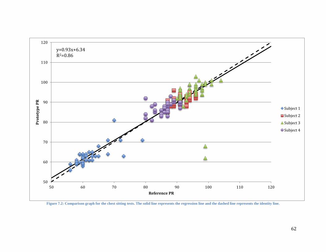
62

Figure 7.2: Comparison graph for the chest sitting tests. The solid line represents the regression line and the dashed line represents the identity line.

50

60

70

80

90

100

110

120

50 60 70 80 90 100 110 120

Pro

toty

pe

PR

Reference PR

Subject 1

Subject 2

Subject 3

Subject 4

y=0.93x+6.34 R2=0.86

63

In Figure 7.3, a comparison plot referencing the data collected from our prototype on the chest of

four different subjects while standing over a six minute period is displayed. The measuring scale ranges

from 80 to 120 bpm with increments of 5 bpm. The linear regression equation and best fit coefficient are

shown at the upper left corner. Similar to the regression line presented in Figure 7.2, the regression line in

this comparison graph shows a slope very close to 1. The statistical coefficient of determination R2, which

is used in the context of statistical modeling for predictions, is a measure of how good a predicted value

might be construed from the modeled values. A lower R2 also shows that the correlation coefficient

denoted as R, is lower than the sitting measurement shown in Figure 7.2.

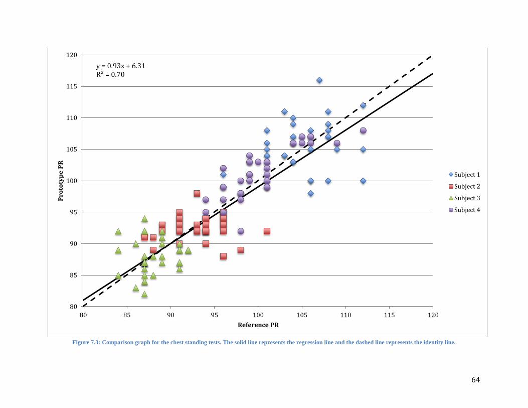
64

Figure 7.3: Comparison graph for the chest standing tests. The solid line represents the regression line and the dashed line represents the identity line.

80

85

90

95

100

105

110

115

120

80 85 90 95 100 105 110 115 120

Pro

toty

pe

PR

Reference PR

Subject 1

Subject 2

Subject 3

Subject 4

y = 0.93x + 6.31 R² = 0.70

65

Figure 7.4 displays a regression line for the PR data collected from our pulse oximeter prototype

on the wrist against the HOMEDICS reference finger pulse oximeter on four different subjects over a six

minute period while sitting. The data are clustered in four different groups, each one having a distinctive

symbol corresponding to the subject tested. The measuring scale ranges from 50 to 120 bpm with

increments of 10 bpm. The total PR data obtained from our prototype for all four subjects ranged from 52

to approximately 105 bpm. The graph displays the linear regression line and R2 on the upper left corner.

In this set of data we observed that the coefficient of variance, R2, and in turn the coefficient of

correlation, R, to be slightly lower than the values observed from the chest while sitting. When visually

comparing the regression line to the line of identity, we can conclude that these measurements were not as

accurate compared to the reference pulse oximeter.

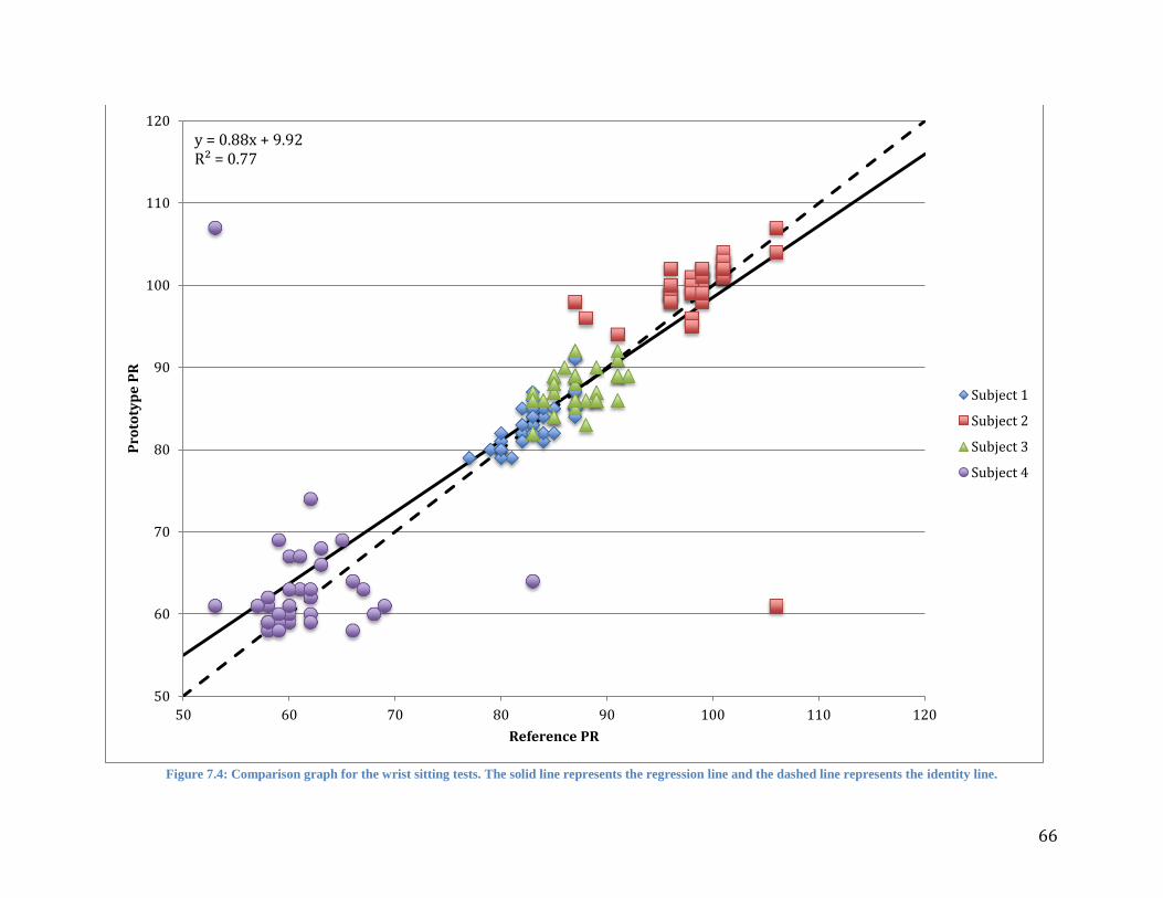
66

Figure 7.4: Comparison graph for the wrist sitting tests. The solid line represents the regression line and the dashed line represents the identity line.

50

60

70

80

90

100

110

120

50 60 70 80 90 100 110 120

Pro

toty

pe

PR

Reference PR

Subject 1

Subject 2

Subject 3

Subject 4

y = 0.88x + 9.92 R² = 0.77

67

In Figure 7.5 a comparison plot referencing the data collected from our prototype on the wrist of

four different subjects over a six minute period while standing is displayed. The measuring scale ranges

from 60 to 120 bpm with increments of 10 bpm. The linear regression equation and best fit coefficient

are shown on the upper left corner. When comparing the standing wrist measurements to the sitting wrist

measurements shown in Figure 7.4, we saw that the measurements obtained from the wrist while standing

appeared to be the least correlated data set. Visually, there appears to be more variations between the

identity line and the regression line than in other comparison graphs.

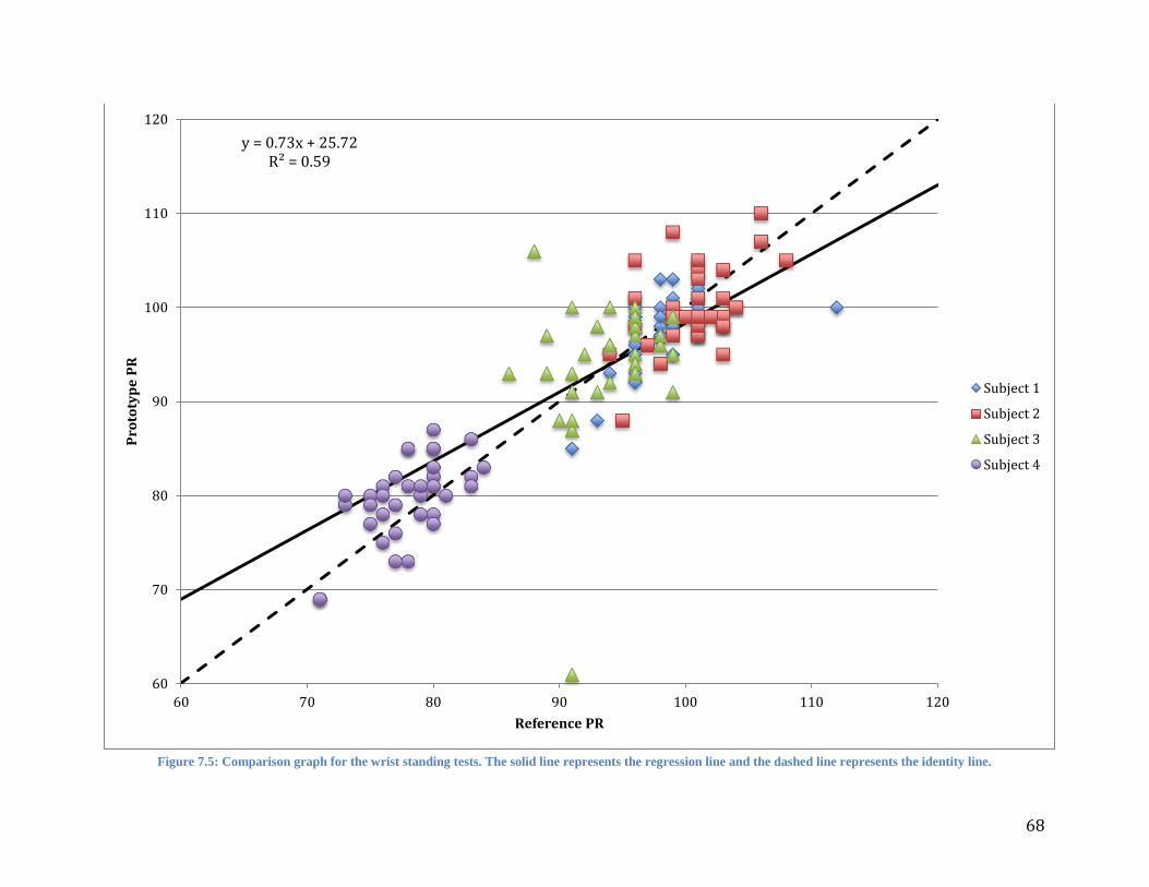
68

Figure 7.5: Comparison graph for the wrist standing tests. The solid line represents the regression line and the dashed line represents the identity line.

60

70

80

90

100

110

120

60 70 80 90 100 110 120

Pro

toty

pe

PR

Reference PR

Subject 1

Subject 2

Subject 3

Subject 4

y = 0.73x + 25.72 R² = 0.59

69

The plot displayed on Figure 7.6 shows the data points collected from our prototype on the wrist

of four different subjects over a six minute period with the HOMEDICS reference device attached to the

finger while hyperventilating. The measuring scale ranges from 50 to 140 bpm with increments of 10

bpm. The linear regression equation and best fit coefficient are shown at the upper left corner. One

characteristic that is quickly observed when looking at this graph is that there is a lower accuracy in these

measurements than in the previous graphs. This is visible in how the data points are distributed and the

distance between points. Another aspect of these graphs that was noticed was that there appeared to be

more outliers present in the data than in the other data sets.

70

Figure 7.6: Comparison graph for hyperventilation tests

50

60

70

80

90

100

110

120

130

140

70 80 90 100 110 120 130 140

Pro

toty

pe

PR

Reference PR

Subject 1

Subject 2

Subject 3

Subject 4

y = 0.8849x + 10.442 R² = 0.56421

71

The hypoxia testing graph shown in Figure 7.7 was performed on 2 subjects capable of holding

their breath for more than 40 seconds. SpO2 readings were collected by our prototype pulse oximeter as

well as by the reference HOMEDICS device. The measuring percentage scale ranged from 90 to 100 with

increments of 1%. Regression line equation and best fit line coefficient are given at the upper left corner.

For the purpose of plotting a regression line for SpO2 we found it very difficult to correctly plot a

regression line when the data had only a 10% range. Considering that for the majority of testing the

subjects maintained a SpO2 level of 97 or 98% we were only able to measure several small dips to assess

the responsiveness of our device to changing SpO2 levels. To correctly plot a regression line, one would

need to change the SpO2 levels over a larger range such as 70-100% in order to have a better idea of how

well our device compares to the reference pulse oximeter.

72

Figure 7.7: Comparison graph for hypoxia tests. The solid line represents the regression line and the dashed line represents the identity line.

90

91

92

93

94

95

96

97

98

99

100

90 91 92 93 94 95 96 97 98 99 100

Pro

toty

pe

Sp

O2

Reference SpO2

Subject 1

Subject 2

y = 0.33x + 64.84 R² = 0.17

73

Dynamic Response Plots 7.2 Dynamic response plots were utilized in analyzing the data because they show the prototype’s response to

changing levels of PR and SpO2 over time. These plots in particular were utilized for all of the

measurements to better understand how our device reacts to varying PR. The fact that the SpO2 levels

varied very little in most of the measurements doesn’t provide any real indication as to whether the

prototype is able to response to changing levels of SpO2. To address this, we performed hypoxia tests in

which we saw the SpO2 level drop to around 90 and plotted those results.

Figures 7.8 and 7.9 depict the SpO2 and PR measurements during the 6 minute testing period

respectively. Although the only information we can obtain from Figure 7.8 is that the SpO2 remained

constant throughout the entire measurement, Figure 7.9 shows the prototypes response to changing levels

of PR. One feature that was observed was that at times when the PR would ramp up, the prototype would

instead ramp downwards towards a smaller PR. In fact, it was observed that this occurred 5 times during

the measurement period.

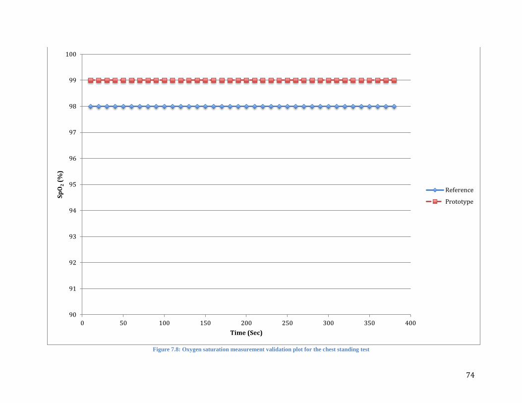
74

Figure 7.8: Oxygen saturation measurement validation plot for the chest standing test

90

91

92

93

94

95

96

97

98

99

100

0 50 100 150 200 250 300 350 400

Sp

O2 (

%)

Time (Sec)

Reference

Prototype

75

Figure 7.9: Pulse rate measurement validation plot for the chest standing test

90

95

100

105

110

115

120

0 50 100 150 200 250 300 350 400

PR

(b

pm

)

Time (Sec)

Reference

Prototype

76

Figures 7.10 and 7.11 display the dynamic response plots for the chest measurements of one

subject while sitting. Although it was observed that the prototype’s measurements bounced around 98%

and 99%, this still doesn’t give us any real interpretations as to how the prototype can handle different

values of SpO2. Figure 7.11 displays the changing PR measurements over time, depicts the variations in

PR of an individual at rest. We did notice from this chart that while our prototype appeared to be

following the general trend of data and PR variability, there was indeed quite a number of errors in the

measurements. Some cases of overshooting and undershooting were observed as well as certain data

points which appeared to almost be delayed PR values of the reference pulse oximeter.

77

Figure 7.10: Oxygen saturation measurement validation plot for the chest sitting test

90

91

92

93

94

95

96

97

98

99

100

0 50 100 150 200 250 300 350 400

Sp

O2(%

)

Time (Sec)

Reference

Prototype

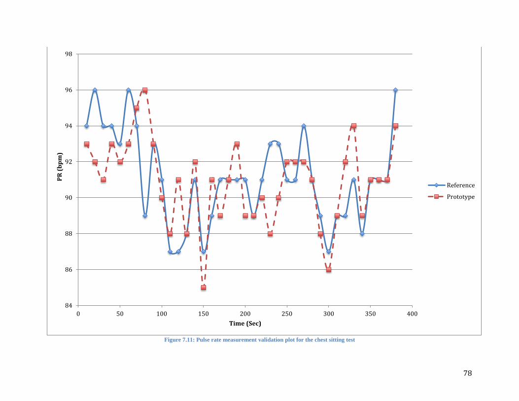
78

Figure 7.11: Pulse rate measurement validation plot for the chest sitting test

84

86

88

90

92

94

96

98

0 50 100 150 200 250 300 350 400

PR

(b

pm

)

Time (Sec)

Reference

Prototype

79

Figures 7.12 and 7.13 display the dynamic response plots for the hyperventilation trials. Both

figures display varying PR’s for two subjects during the 6 minute measurement period. Plot 1, depicted as

Figure 7.12 shows a very high correlation between the prototype and the reference pulse oximeter. This is

evident in the proximity of the data points between the prototype and reference pulse oximeter as well as

the general trend that the chart follows. However, it was noticed that at 80 seconds, there was an

unexplained drop in PR from the 75-80 range to a PR value of 53. The reason for this was believed to be

due to corrupted PPG signals during that 10 second duration of measurements. Figure 7.1 shows how a

corrupted PPG signal appears. Since our method for calculating PR is by searching for the highest

amplitude around a specific frequency, any high frequency noise presented either through ambient light

picked up by the sensor or by motion artifacts would slant the power spectrum of the signal which in turn

would provide false PR calculations for that interval of data. Figure 7.13 shows similar drops in PR as

well due to corrupted PPG signals. One difference observed in Figure 7.13 was that the data were not as

closely correlated as in Figure 7.12.

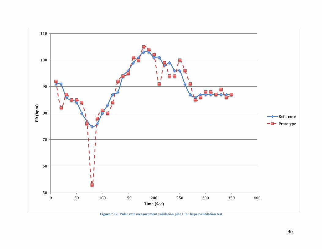
80

Figure 7.12: Pulse rate measurement validation plot 1 for hyperventilation test

50

60

70

80

90

100

110

0 50 100 150 200 250 300 350 400

PR

(b

pm

)

Time (Sec)

Reference

Prototype

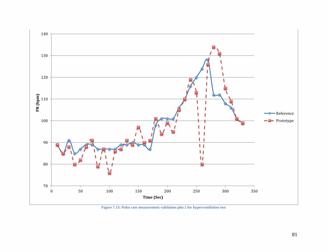
81

Figure 7.13: Pulse rate measurement validation plot 2 for hyperventilation test

70

80

90

100

110

120

130

140

0 50 100 150 200 250 300 350

PR

(b

pm

)

Time (Sec)

Reference

Prototype

82

Figures 7.14 and 7.15 depict the PR and SpO2 measurements during the 6 minute testing period

from the wrist as the subject was sitting, respectively. Figure 7.14 shows the prototypes response to

changing levels of PR. In general this set of data appears to be very closely correlated and only contains

one measurement in which the PR overshoots the reference by about 4bpm. In Figure 7.15 we can

observe a small dip at the beginning of the measurements in the SpO2 but otherwise, the SpO2 levels

stayed constant throughout the entire measurement.

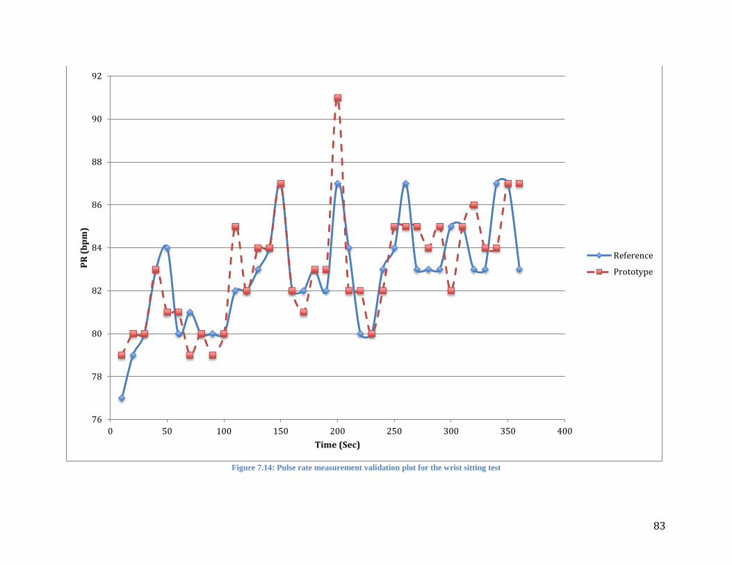
83

Figure 7.14: Pulse rate measurement validation plot for the wrist sitting test

76

78

80

82

84

86

88

90

92

0 50 100 150 200 250 300 350 400

PR

(b

pm

)

Time (Sec)

Reference

Prototype

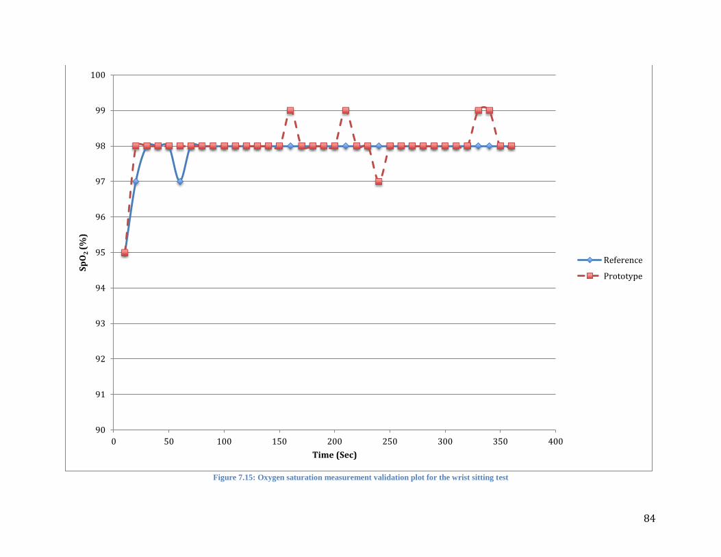
84

Figure 7.15: Oxygen saturation measurement validation plot for the wrist sitting test

90

91

92

93

94

95

96

97

98

99

100

0 50 100 150 200 250 300 350 400

Sp

O2

(%

)

Time (Sec)

Reference

Prototype

85

Figures 7.16 and 7.17 depict the SpO2 and PR measurements during the 6 minute testing period

from the wrist as the subject was standing. In Figure 7.16 we observe a constant bouncing of SpO2

between 98 and 99% for our prototype and a dip in SpO2 at around 2 minutes into the measurements.

Figure 7.17 shows the prototypes response to changing levels of PR while the subject was standing. Apart

from two moments of undershooting in which the value displayed on the prototype was lower than the

value displayed on the reference device, the rest of the data appeared to be slightly less well correlated

than when the subject was sitting.

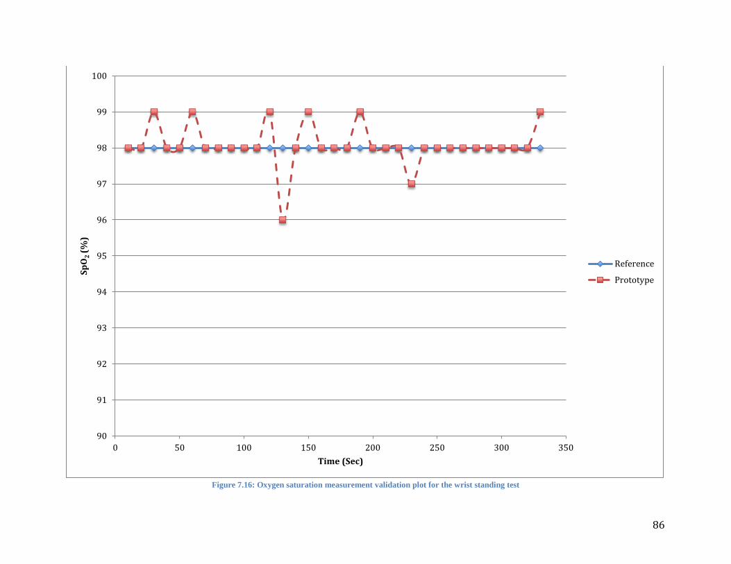
86

Figure 7.16: Oxygen saturation measurement validation plot for the wrist standing test

90

91

92

93

94

95

96

97

98

99

100

0 50 100 150 200 250 300 350

Sp

O2

(%

)

Time (Sec)

Reference

Prototype

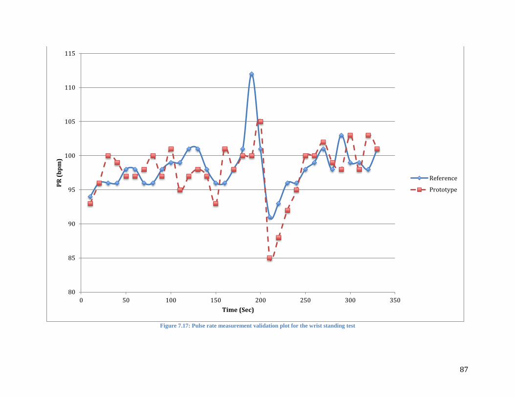
87

Figure 7.17: Pulse rate measurement validation plot for the wrist standing test

80

85

90

95

100

105

110

115

0 50 100 150 200 250 300 350

PR

(b

pm

)

Time (Sec)

Reference

Prototype

88

To accurately see how well our device responded to sudden drops in SpO2 we asked our subjects

to hold their breaths for 45 seconds in hopes that a drop in SpO2 could be observed. Figures 7.18 and 7.19

display two separate plots for induced hypoxia. In Figure 7.18 the moment of induced hypoxia can be

observed at around 120-160 seconds in which the SpO2 dropped from 99 to 91% in the reference pulse

oximeter and 97 to 93% for the prototype. While the drop in SpO2 for the prototype was not as sudden as

it was for the reference pulse oximeter, it does in fact validate the claim that our prototype does respond

to changing levels of SpO2. In Figure 7.19 we observe two moments of induced hypoxia, once at 150

seconds and later at 230 seconds. We also observed what appeared to be a delay between our prototype

and the reference pulse oximeter when the drops in SpO2 occurred.

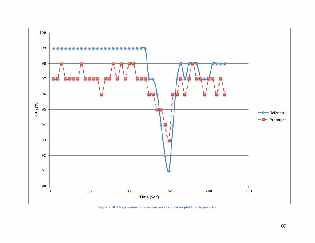
89

Figure 7.18: Oxygen saturation measurement validation plot 1 for hypoxia test

90

91

92

93

94

95

96

97

98

99

100

0 50 100 150 200 250

Sp

O2

(%

)

Time (Sec)

Reference

Prototype

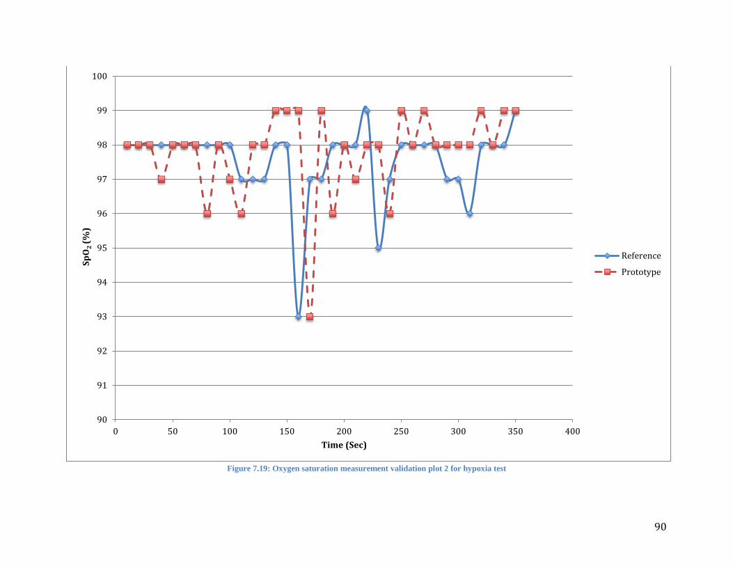
90

Figure 7.19: Oxygen saturation measurement validation plot 2 for hypoxia test

90

91

92

93

94

95

96

97

98

99

100

0 50 100 150 200 250 300 350 400

Sp

O2

(%

)

Time (Sec)

Reference

Prototype

91

Residual Plots 7.3

Residual plots were also utilized in analyzing the hypoxia and hyperventilation tests. To graph the

residual plots, we calculated the average between the observed measurements from the reference device

and our prototype, the difference between each observed measurement, the average of the difference

between each observed measurement number, and the standard deviation of the differences. Using these

calculations we then plotted the averages of the individual measurements on the horizontal axis and the

difference between measurements on the vertical axis. A solid black line was then plotted to represent the

average of the differences, and two dashed black lines to represent + 2 standard deviations around the

average of the difference of measurements. Figures 7.20, 7.21 and 7.22 show the residual plots for the

hyperventilation testing. All of these plots show that at least 95% of the data falls within the two standard

deviations meaning that the differences between the reference device and the prototype are normally

distributed. Although 95% of the data in each figure does fall within the two standard deviations, Figure

7.22 shows the best representation of a high correlation between the reference device and the prototype.

Most of the data shown in that plot is much closer to the average of the differences, shown as the black

solid line.

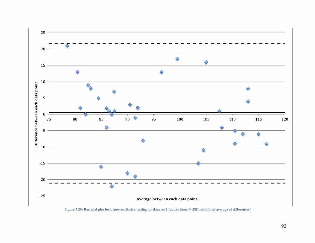
92

Figure 7.20: Residual plot for hyperventilation testing for data set 1 (dotted lines: + 2SD, solid line: average of differences)

-25

-20

-15

-10

-5

0

5

10

15

20

25

75 80 85 90 95 100 105 110 115 120

Dif

fere

nce

be

twe

en

ea

ch d

ata

po

int

Average between each data point

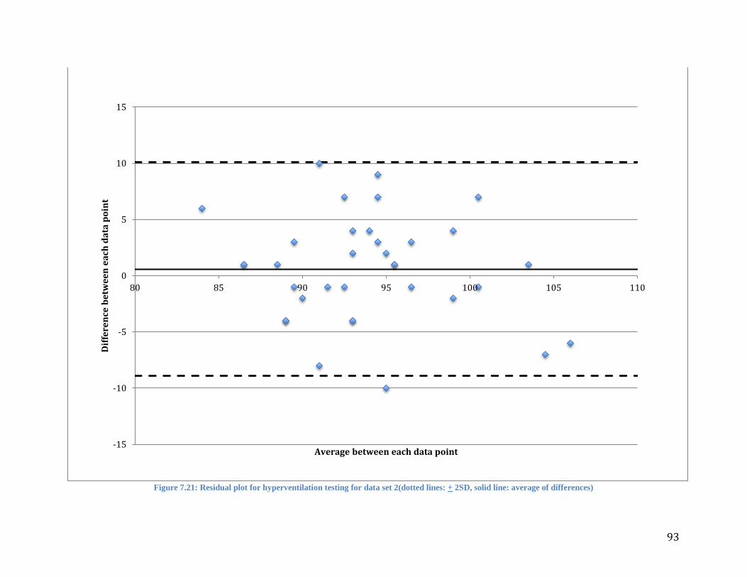
93

Figure 7.21: Residual plot for hyperventilation testing for data set 2(dotted lines: + 2SD, solid line: average of differences)

-15

-10

-5

0

5

10

15

80 85 90 95 100 105 110

Dif

fere

nce

be

twe

en

ea

ch d

ata

po

int


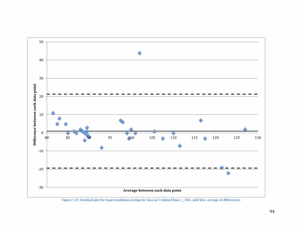
94

Figure 7.22: Residual plot for hyperventilation testing for data set 3 (dotted lines: + 2SD, solid line: average of differences)

-30

-20

-10

0

10

20

30

40

50

80 85 90 95 100 105 110 115 120 125 130

Dif

fere

nce

be

twe

en

ea

ch d

ata

po

int


95

Figures 7.23 and 7.24 show the residual plots for the hypoxia testing. The data in both plots

appear to be slanted to one side due to there not being a large enough SpO2 range to effectively measure.

However, one positive to note from these plots is that the majority of the residuals in both plots appear to

fall within two standard deviations of the average difference.

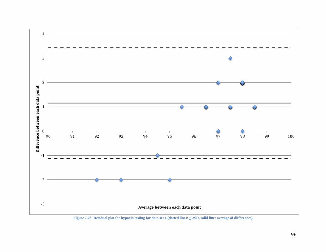
96

Figure 7.23: Residual plot for hypoxia testing for data set 1 (dotted lines: + 2SD, solid line: average of differences)

-3

-2

-1

0

1

2

3

4

90 91 92 93 94 95 96 97 98 99 100

Dif

fere

nce

be

twe

en

ea

ch d

ata

po

int


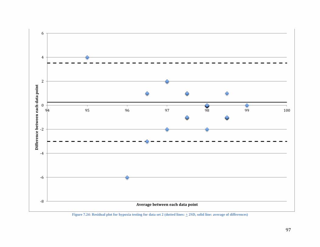
97

Figure 7.24: Residual plot for hypoxia testing for data set 2 (dotted lines: + 2SD, solid line: average of differences)

-8

-6

-4

-2

0

2

4

6

94 95 96 97 98 99 100

Dif

fere

nce

be

twe

en

ea

ch d

ata

po

int


98

8 Discussion When creating a device such as a pulse oximeter which requires the acquisition of signals such as PPGs, it

is difficult to ensure the integrity of the signals that are acquired. This causes the placement of the sensor

on the wrist and chest to be very important. We were able to obtain fairly strong PPGs from the wrist and

chest because of the stronger signals due to the high levels of bone and subcutaneous tissues in these

locations.

The summarized results suggest that recorded wrist measurements were more accurate than chest

measurements. For the standing and sitting measurement tests obtained from the wrist, the errors obtained

were 0.6%, and 0.2% for SpO2 and 0.2%, 1.1% for the PR, respectively. While the measurements from

the chest obtained errors of 0.4% and 0.3% for SpO2 and 0.1%, and 0.7% for the PR, respectively for the

same test conditions. There are many factors that could contribute to the difference in the percent errors

for the two different locations. When the sensor was placed on the wrist, it was placed over the radial

artery which could have given stronger signals as opposed to those gathered from the chest where the

sensor was simply placed over the sternum. One factor noticed was when the sensor is placed on the

chest, the device became subject to increased motion artifact from breathing. The motion the chest makes

when each subject took a breath in some cases moved the device on the skin and could have also

prevented it from being in constant contact with the skin. Another factor that could have affected this is

the pressure at which the device was strapped on. If there was too much or too little pressure, the signal

strength could change, in turn changing the results. For this device to be considered a success, the percent

error for all tests must remain at ±3. Although these factors did not affect the accuracy of the device in an

extremely negative way as displayed in the results, they were cause for a slightly higher percent error in

data taken from the chest. In these cases it was noticed the sensor would allow ambient light to be picked

up by the photodetectors. It was observed that when this occurred, the sensor output would completely

saturate due to the high amplification we utilized for signal analysis.

The standard tests of standing and sitting while taking measurements from the chest and wrist

showed that the prototype could accurately and continuously measure SpO2 and PR. While the hypoxia

and hyperventilation tests demonstrated that the prototype can respond to various SpO2 and PR

measurements respectively. The comparison graphs were used to plot each set of data for each test on one

graph together. In these graphs, the reference device was plotted against our prototype to see the

correlation between the two. Each different marker corresponds to a different subjects’ data taken. The

identity line represents a line with a slope of 1. This was useful to plot in the comparison charts because it

represents the slope our data is expected to follow when comparing devices as such. The regression line in

these plots models the relationship between the reference device and our prototype. In figures 7.2 and 7.3

99

displaying PR data, the regression line has a slope of .93 and .93 respectively. These slopes show the high

correlation between the reference device and our prototype for both the chest sitting and standing results

when measuring PR. In figures 7.4 and 7.5 displaying PR data, the regression lines have a slope of .89

and .73 respectively, also showing a high correlation between the reference device and our prototype for

the wrist sitting and standing when measuring PR. When testing the devices ability to detect changing PR

and SpO2, the group only took measurements from the wrist. This was decided because of the increased

accuracy in the measurements taken from the wrist. Figure 7.6 displays the PR data for the

hyperventilation testing. The slope of the regression line here is .88 showing that our device is able to

accurately detect changes in PR that would mimic those of exercise. Figure 7.7 displays the SpO2 data for

hypoxia testing. The slope of the regression line here is .33 which would normally indicate that the device

does not have a high correlation with the reference device however, because SpO2’s measurements are on

such a small scale, even the slightest of discrepancies would cause a big change in the slope of the

regression line. It is for examples like this that it was necessary to analyze the data in more than one way

and to have more than one form of graphical representation.

The dynamic response plots were used to see the prototypes response to PR and SpO2 as opposed

to the reference devices response over time. Each graph contains a line representing the prototype and a

line representing the reference device. While the plots here for the chest while sitting and standing and the

wrist while sitting and standing show that the measurements from our prototype remain in close proximity

to those of the reference device, the most valuable plots are those done for hyperventilation and hypoxia.

Figures 7.12 and 7.13 show that the prototype can react to changing levels of PR as fast as the reference

device does and with high accuracy. In figure 7.12 at about 75 seconds in and in figure 7.13 at about 250

seconds there are noticeable outliers in the PR measurement from the prototype. The outliers for each

subject went from a regular PR, around 90bpm, to values of about 40 or 50bpm. To verify whether this

was due to abnormal PPG data or the software, the PPG data gathered by the VI was re-examined for the

specific periods of time in which the outliers occurred. It was discovered that these outliers were

primarily due to corrupted PPG data. Figure 7.1 shows a portion of the PPG data with corrupted readings

which could be due to motion artifacts introduced by the subject through sudden movements. Another

possibility for the corrupted data could be related to the amount of pressure applied to the sensor when it

was placed on the subject. Figure 7.18 shows one drop in SpO2 during induced hypoxia at about 150

seconds while figure 7.19 shows two drops in SpO2 during induced hypoxia at 160 seconds and at 230

seconds. Both the prototype and the reference oximeter registered the drops in oxygen saturation, though

the drop observed by our prototype was less than that of the reference device. This test demonstrated the

prototype’s ability to detect a decrease in SpO2 with some degree of accuracy.

100

Residual plots were used to show by how much the prototype is likely to differ from the reference

device. These plots allow us to see if there are any large discrepancies between the reference device and

the prototype that would otherwise not be seen in the comparison charts. Figure 7.22 shows one of the

residual plots for hyperventilation testing. In this plot we can see that there is not a large difference in the

data gathered from the reference device and the prototype as all the data is fairly close to 0 and well

within the 2 standard deviation limits showing that our data is normally distributed. Figures 7.20 and 7.21

show the remaining two residual plots for hyperventilation. These two plots show a much larger range of

difference between the reference device and the prototype however, 95% of the values are within the 2

standard deviation limits and that the data is normally distributed as well. Figures 7.23 and 7.24 show the

residual plots for hypoxia testing. These two plots show that the differences between the reference device

and the prototype are very small ranging from a difference of either 1 or 2 and shows that 95% of these

data points are also within the 2 standard deviation limit showing that our data is normally distributed.

From the data presented in Table 7.2, the accuracy of the PR measurements ranged in percent

error between 3-5% for every single data set. From this it was concluded that while the tone

measurements function in LabVIEW is a simple and effective method for calculated PR, it introduces a

high degree of error since it is programmed to seek the highest amplitude frequency. For SpO2 a low

percent error was maintained for all the stationary measurements, but there was a decrease in accuracy

when the prototype was experiencing changing SpO2 levels. To ascertain a more precise accuracy for the

prototype, further testing should be done in which the SpO2 levels range from 70-100%.

101

10 Summary This project started with the goal of designing and building a wearable reflectance-based pulse oximeter

that could measure SpO2 and PR accurately from the chest and wrist. A literature search was the

conducted exploring pulse oximetry theory, application methods, and commercial products. After which,

alternative designs for a reflectance-based pulse oximeter were considered. Assessing the benefits of each

alternative design, a design consisting of 8 photodiodes positioned concentrically around 2 LEDs, one red

and one infrared at wavelengths of 660nm and 940nm, respectively, was selected. In the circuitry, an

Arduino Duo microprocessor was used as the LED driver and the logic driver. Sample-and-Hold circuits

were utilized to separate the appropriate signals for red and infrared light with analog bandpass filters

implemented to isolate the AC component of the PPG waveforms from the DC component. Stages of

operational amplifiers were also used to amplify the original signal created by the sensor and amplify the

AC signals which were representative of the PPG fluctuations.

The software for this project was developed in the program LabVIEW to further filter the signals

and calculate SpO2 and PR. For the calculation of PR, tone measurement function was used inside of

LabVIEW which searches for the highest amplitude signal around a custom set frequency. Expecting the

frequency of the range of PRs to lie between 1Hz and 3Hz, the function was set to search around 2Hz

with a window of + 50%. This method was very effective in calculating the PR frequency and chose to

stay with it rather than opting for a peak to peak analysis. The PR frequency was then multiplied by 60 to

have the final PR values in beats per minute.

For the calculation of SpO2 several functions inside of LabVIEW were used to obtain these

values. For the AC signals, a function called AC & DC estimator which effectively measured the

amplitude of every single amplified PPG fluctuation and then averaged this amplitude over 10 seconds

worth off PPG data. To obtain a DC value for both red and infrared signals, the amplitude and level

measurements function was used to average 10 seconds worth of data and come up with a constant value

for the DC. These methods were found to be satisfactory for calculating the red and infrared AC and DC

values due to the small variation in the signal once placed on the skin of an individual. Variations in the

signal were only noticeable if the sensor was moved or if the subject moved during testing. For

calculating SpO2, equation 2 was used with variables A= 110 and B = -25. The value for SpO2 was then

normalized so that it is out of 100% and then plotted on a chart as well as having a visual gauge as a

reference with a range from 0-100% SpO2.

Tests were performed using our prototype and a HOMEDICS Deluxe Pulse Oximeter as a

reference. For the chest measurements, the sensor was placed directly over the sternum while for the wrist

measurements the sensor was worn on the left arm over the radial artery. Depending on the signal

102

intensity for each subject there were variations in the specific location over the radial artery in which the

sensor was placed on to collect measurements. The pressure of the sensor on the skin was adjusted using a

Velcro strap which went around the wrist and chest. The testing performed allowed for the collection of

measurements from the chest and wrist while sitting and standing. Tests of hypoxia and hyperventilation

were also performed to observe the responds of the prototype to changing levels of SpO2 and PR. Many

of the subjects had trouble holding their breaths for the allotted 45 seconds thus the lowest SpO2 levels

observed were 91%. From the gradual increase and decrease of PR, the prototypes response to changing

PRs was observed. The VI was set to sample at 25 samples per second for 250 samples each

measurement. Every 10 seconds, the VI would display 10 seconds worth of PPG waveforms, as well as

the calculated PR and SpO2 for the last 10 seconds. To maintain the same sampling rate as the prototype,

the SpO2 was also sampled and PR values of the reference pulse oximeter every 10 seconds to coincide

with the results picked up by the VI.

Once all of the measurements were taken, the data were analyzed using several different

techniques. The averages of each data set were taken for both measurants from which the accuracy of the

prototype to that of the reference pulse oximeter was calculated and comparative graphs were created.

Regression lines were also calculated and plotted for each set of measurements and compared to an

identity line with a slope of 1 and a y-intercept of 0.

The hypoxia and hyperventilation measurements demonstrated how the device would perform

with changing SpO2 and PR levels. To this effect, dynamic response graphs were plotted for each

measurement. For the hypoxia and hyperventilation tests, respective prototype and reference pulse

oximeter SpO2 values over time were plotted. Induced hypoxia resulted in lowered levels of SpO2 and

showing a similar response in both the prototype and the reference pulse oximeter. During

hyperventilation, rising PR on each subject were observed with the prototype and reference pulse

oximeter. Lastly, residual plots were also created for the hypoxia and hyperventilation tests to investigate

how our device differs from the reference device. This was accomplished by calculating the difference

between the prototype and reference pulse oximeter for each measurement.

103

11 Conclusion Based on the experimental results derived several conclusions can be drawn. Through the testing

performed on the prototype pulse oximeter we observed that it is in fact possible to measure SpO2 and PR

from the wrist and chest with a reasonable level of accuracy. The SpO2 measurement contained an error

of less than +1% and the PR measurements less than +4%. However the prototype does still need some

improvement to increase the accuracy of the PR. Though simple to implement, the algorithm currently

being used in calculating PR did not provide the level of accuracy required for a FDA regulated

commercial device.

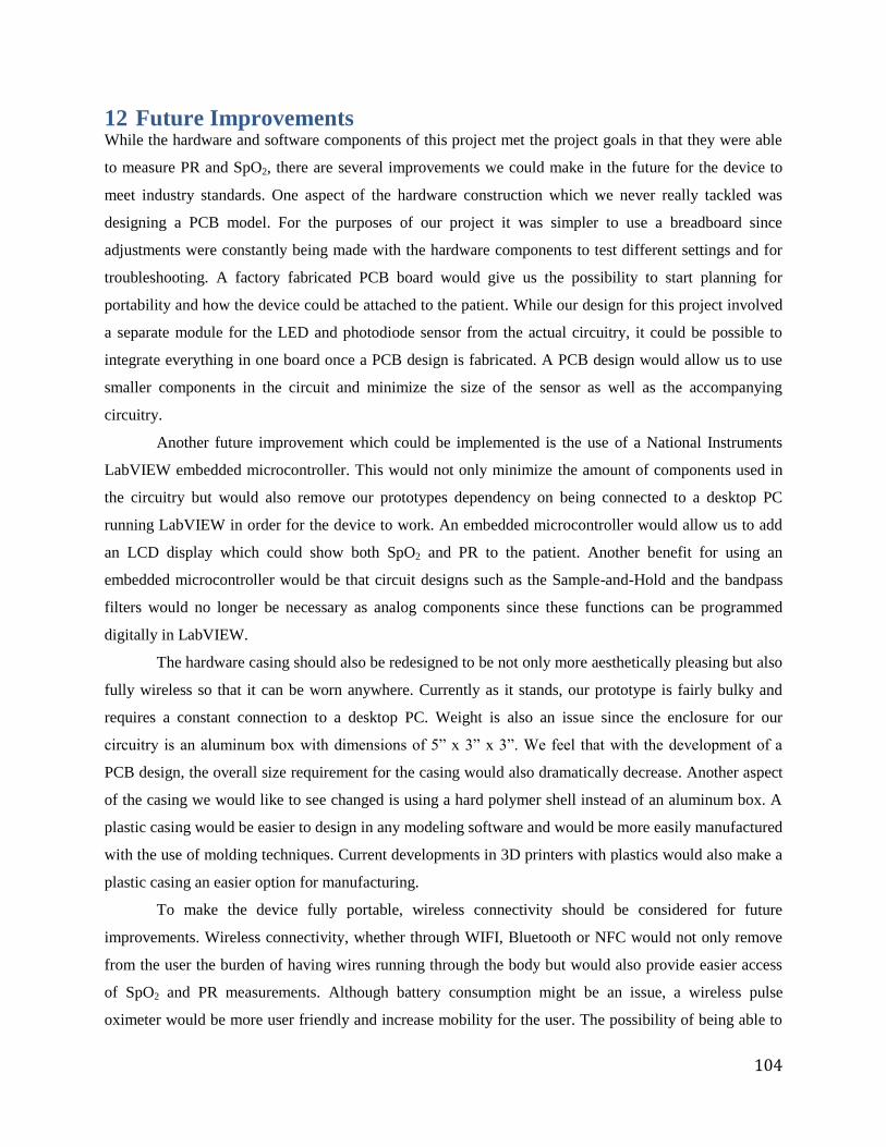
104

12 Future Improvements While the hardware and software components of this project met the project goals in that they were able

to measure PR and SpO2, there are several improvements we could make in the future for the device to

meet industry standards. One aspect of the hardware construction which we never really tackled was

designing a PCB model. For the purposes of our project it was simpler to use a breadboard since

adjustments were constantly being made with the hardware components to test different settings and for

troubleshooting. A factory fabricated PCB board would give us the possibility to start planning for

portability and how the device could be attached to the patient. While our design for this project involved

a separate module for the LED and photodiode sensor from the actual circuitry, it could be possible to

integrate everything in one board once a PCB design is fabricated. A PCB design would allow us to use

smaller components in the circuit and minimize the size of the sensor as well as the accompanying

circuitry.

Another future improvement which could be implemented is the use of a National Instruments

LabVIEW embedded microcontroller. This would not only minimize the amount of components used in

the circuitry but would also remove our prototypes dependency on being connected to a desktop PC

running LabVIEW in order for the device to work. An embedded microcontroller would allow us to add

an LCD display which could show both SpO2 and PR to the patient. Another benefit for using an

embedded microcontroller would be that circuit designs such as the Sample-and-Hold and the bandpass

filters would no longer be necessary as analog components since these functions can be programmed

digitally in LabVIEW.

The hardware casing should also be redesigned to be not only more aesthetically pleasing but also

fully wireless so that it can be worn anywhere. Currently as it stands, our prototype is fairly bulky and

requires a constant connection to a desktop PC. Weight is also an issue since the enclosure for our

circuitry is an aluminum box with dimensions of 5” x 3” x 3”. We feel that with the development of a

PCB design, the overall size requirement for the casing would also dramatically decrease. Another aspect

of the casing we would like to see changed is using a hard polymer shell instead of an aluminum box. A

plastic casing would be easier to design in any modeling software and would be more easily manufactured

with the use of molding techniques. Current developments in 3D printers with plastics would also make a

plastic casing an easier option for manufacturing.

To make the device fully portable, wireless connectivity should be considered for future

improvements. Wireless connectivity, whether through WIFI, Bluetooth or NFC would not only remove

from the user the burden of having wires running through the body but would also provide easier access

of SpO2 and PR measurements. Although battery consumption might be an issue, a wireless pulse

oximeter would be more user friendly and increase mobility for the user. The possibility of being able to

105

display these measurements on any smartphone or other portable wireless devices is another advancement

that could make this device increasingly valuable for patients and clinicians.

106

References

(1) Mendelson, Y. “Pulse Oximetry.” Wiley Encyclopedia of Biomedical Engineering (2006): vol. 5. Hoboken,

NJ: John Wiley & Sons, Inc. Print.

(2) Pole, Yash. "Evolution of the Pulse Oximeter." International Congress Series 1242 (2002): 137-44. Print.

(3) "Hemoglobin." Encyclopædia Britannica. Encyclopædia Britannica Online Academic Edition. Encyclopædia

Britannica Inc., 2012. Web. 15 Sep. 2012.

<http://www.britannica.com/EBchecked/topic/260923/hemoglobin>.

(4) Brinkman R., Zijlstra W.G., and Koopmans R.K, “A Method For Continuous Observation Of Percentage O2

Saturation In Patients,” Arch. Chir. Neerl. 1 (1950): 333 - 444. Print.

(5) Mendelson, Y., and B. D. Ochs. "Noninvasive Pulse Oximetry Utilizing Skin Reflectance

Photoplethysmography." IEEE transactions on bio-medical engineering (1988): 35, 10, 798-805. Print.

(6) Mendelson, Duckworth, and Comtois. “A wearable reflectance pulse oximeter for remote physiological

monitoring.” Conference Proc. IEEE Engineering Medical Biology Soc. (2006): 1:912-5. Print.

(7) Santa Medical. Finger pulse oximeter SM-110 with carry case and neck wrist cord.

(8) Mendelson, Y., et al. "Design and Evaluation of a New Reflectance Pulse Oximeter Sensor." Medical

instrumentation 22.4 (1988): 167. Print.

(9) Shelley K. and Shelley S., “Pulse Oximeter Waveform: Photoelectric Plethysmography,” Clinical

Monitoring, Carol Lake, R. Hines, and C. Blitt, Eds.: W.B. Saunders Company, (2001): 420-428. Print.

(10) Shelley K. H., Jablonka D. H., Awad A. A., Stout R. G., Rezkanna H., and Silverman D. G., “What Is the

Best Site for Measuring the Effect of Ventilation on the Pulse Oximeter Waveform?” Anesth Analg, (2006):

vol. 103, 372-377. Print.

(11) Reisner A, Shaltis. P. A., McCombie D., and Asada, H. H., “Utility of the Photoplethysmogram in

Circulatory Monitoring, Anesthesiology,” Anesthesiology, (2008): vol. 108, pp. 950-958. Print.

(12) Nogawa, M., Kaiwa, T., and Takatani, S., "A Novel Hybrid Reflectance Pulse Oximeter Sensor With

Improved Linearity And General Applicability to Various Portions of the Body," Engineering in Medicine

and Biology Society, (1998). Proceedings of the 20th Annual International Conference of the IEEE,

vol.4,.1858-1861.

(13) Tilakaratna, Prasanna. "Pulse Oximeter." Equipmentexplained.com. N.p., n.d. Web. 15 Sept. 2012.

<http://www.equipmentexplained.com/physics/respi_measurements/oxygen/oximeter/pulse_oximeter

.html>.

(14) Dresher RP, Mendelson Y., “Reflectance Forehead Pulse Oximetry: Effects of Contact Pressure During

Walking.” Conf Proc IEEE Eng Med Biol Soc. (2006); 1: 3529-32.

(15) Mardirossian, G., and Schneider R. E.. "Limitations of Pulse Oximetry." Anesthesia Progress 39.6 (1992):

194-6. Print.

(16) Cocker, B., Leung J., Cohen C., Goska B., Albright R., House S., and Chiang P.. "Wearable, Wireless

Reflectance-Sensing Pulse Oximeter." (2012): 2017-020.

(17) "Neonatal Pulse Oximetry Archives Tag Archive for Baby Heart Screening- Newborn Heart Defect

Screening." Baby Heart Screening Newborn Heart Defect Screening. N.p., n.d. Web. 23 Apr. 2013.

(18) Online Courses: Medical Equipment Technology, Support and Management. N.p., n.d. Web. 23 Apr. 2013.

(19) Anliker et al. “AMON: A Wearable Multiparameter Medical Monitoring and Alert System.” IEEETrans Inf

Technology Biomedical (2004): (4) 415-27. Print.

(20) Mendelson, Y., and M. J. McGinn. "Skin reflectance pulse oximetry: In vivo measurements from the

forearm and calf." Journal of Clinical Monitoring and Computing 7.1 (1991): 7-12.

(21) Respironics. WristOx™ Ambulatory Finger Pulse Oximeter.

(22) Crucial Medical Systems. Oled cms50d fingertip pulse oximeter and oxygen meter.

(23) Mendelson Y. and Pujary. “Photodetector Size Considerations in the Design of a Noninvasive Reflectance

Pulse Oximeter for Telemedicine Applications.” IEEE Xplore, (2003): 148-149. Print.

(24) Schreiner, C., Catherwood, P., & Anderson, J. “Blood Oxygen Level Measurement with a Chest-Based

Pulse Oximetry Prototype System.” Computing in Cardiology (2010). Print.

(25) Li, K., & Warren, S. “A Wireless Reflectance Pulse Oximeter with Digital Baseline Control for Unfiltered

Photoplethysmograms.” IEEE Transactions on Biomedical Circuit and Systems (2010). Print.

107

Appendix A: Description of LabVIEW Discussed below are the functions used in the construction of the program that was used in this study.

While loop is a structure that allows for the continuous sampling of input signals and the application of

the diagrams placed within it.

Figure A.1: While loop

When placed in the block diagram, the DAQ assistant launches creating a new task. The task was to

identify the signal provided by the external DAQ and set sampling parameters. The task can be edited by

double-clicking the DAQ assistant. For continuous measurement a while loop should be placed around

the DAQ assistant.

Figure A.2: DAQ Assistant

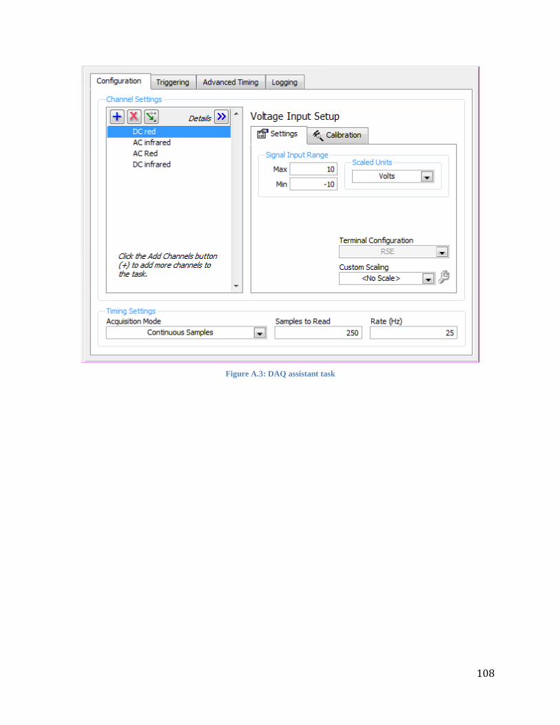
108

Figure A.3: DAQ assistant task

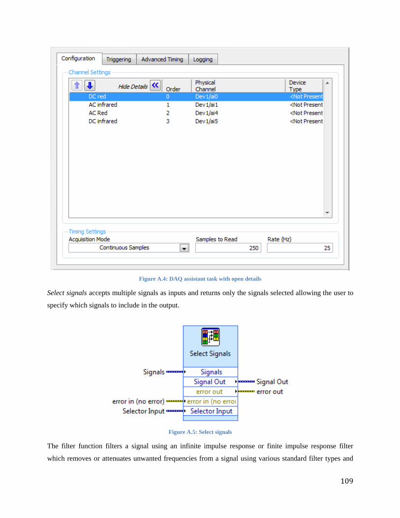
109

Figure A.4: DAQ assistant task with open details

Select signals accepts multiple signals as inputs and returns only the signals selected allowing the user to

specify which signals to include in the output.

Figure A.5: Select signals

The filter function filters a signal using an infinite impulse response or finite impulse response filter

which removes or attenuates unwanted frequencies from a signal using various standard filter types and

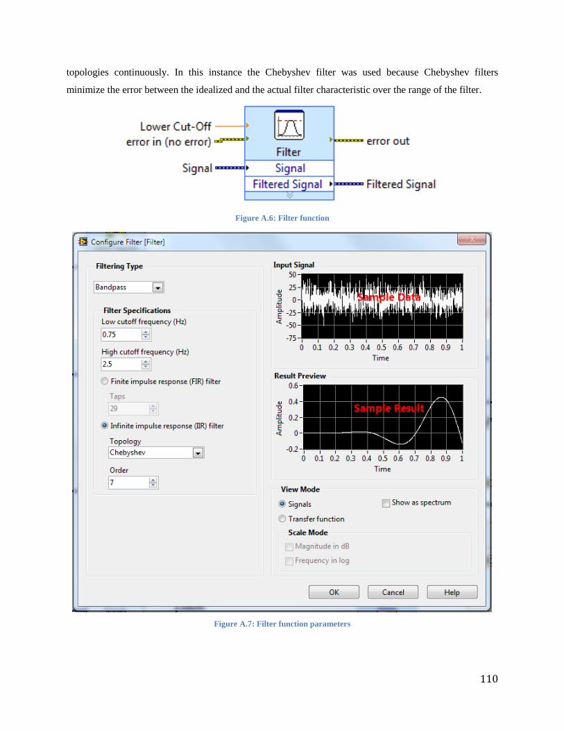
110

topologies continuously. In this instance the Chebyshev filter was used because Chebyshev filters

minimize the error between the idealized and the actual filter characteristic over the range of the filter.

Figure A.6: Filter function

Figure A.7: Filter function parameters

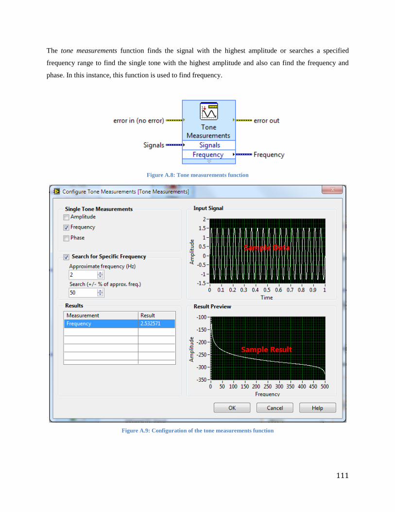
111

The tone measurements function finds the signal with the highest amplitude or searches a specified

frequency range to find the single tone with the highest amplitude and also can find the frequency and

phase. In this instance, this function is used to find frequency.

Figure A.8: Tone measurements function

Figure A.9: Configuration of the tone measurements function

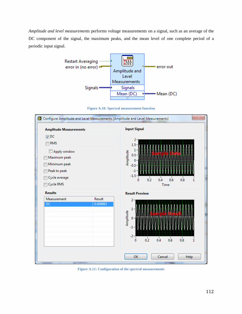
112

Amplitude and level measurements performs voltage measurements on a signal, such as an average of the

DC component of the signal, the maximum peaks, and the mean level of one complete period of a

periodic input signal.

Figure A.10: Spectral measurement function

Figure A.11: Configuration of the spectral measurements

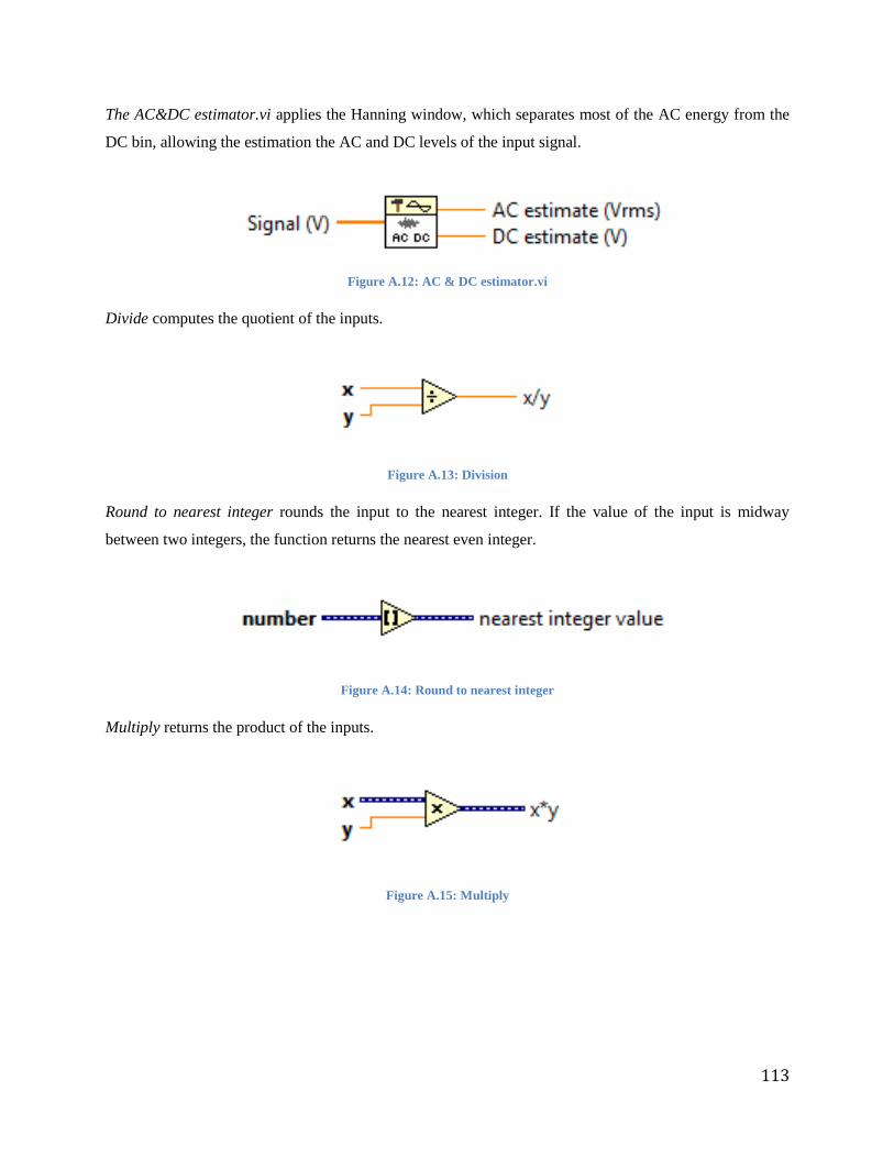
113

The AC&DC estimator.vi applies the Hanning window, which separates most of the AC energy from the

DC bin, allowing the estimation the AC and DC levels of the input signal.

Figure A.12: AC & DC estimator.vi

Divide computes the quotient of the inputs.

Figure A.13: Division

Round to nearest integer rounds the input to the nearest integer. If the value of the input is midway

between two integers, the function returns the nearest even integer.

Figure A.14: Round to nearest integer

Multiply returns the product of the inputs.

Figure A.15: Multiply

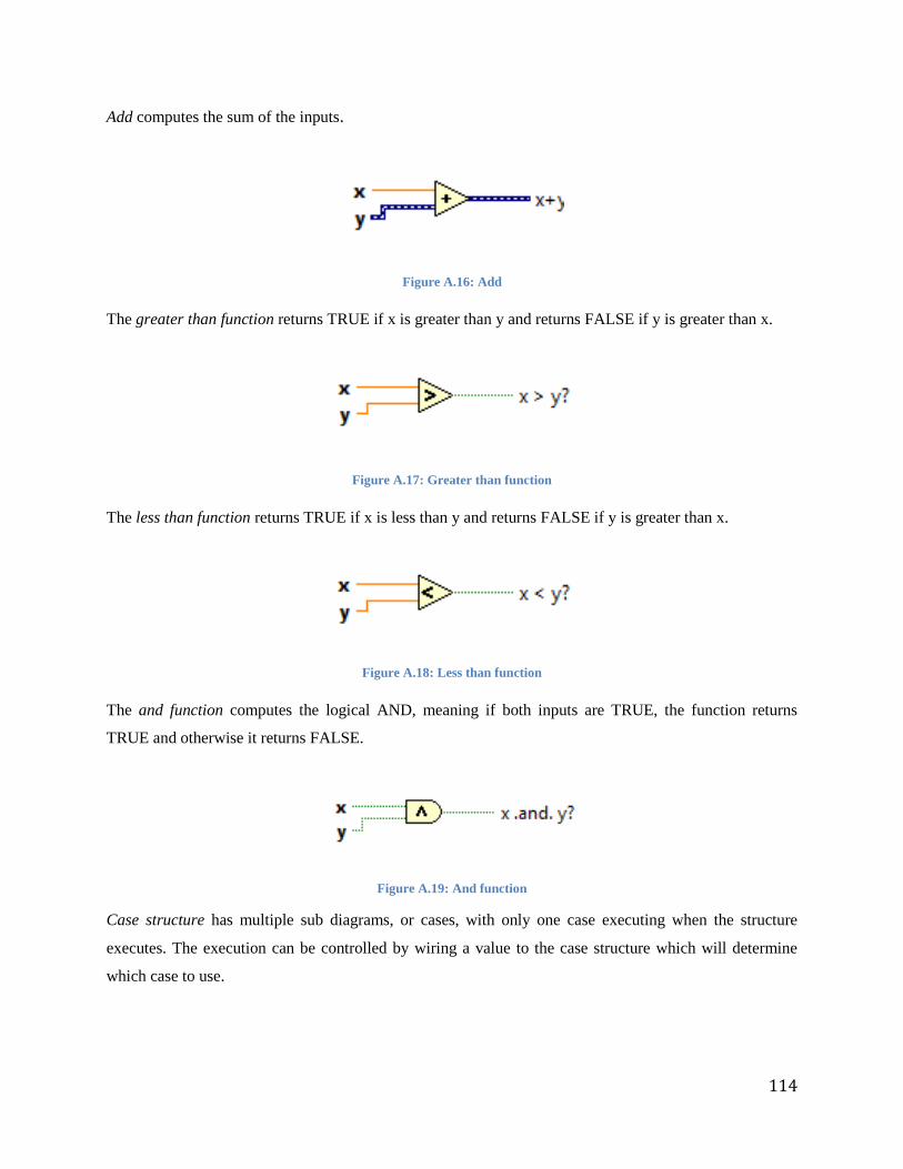
114

Add computes the sum of the inputs.

Figure A.16: Add

The greater than function returns TRUE if x is greater than y and returns FALSE if y is greater than x.

Figure A.17: Greater than function

The less than function returns TRUE if x is less than y and returns FALSE if y is greater than x.

Figure A.18: Less than function

The and function computes the logical AND, meaning if both inputs are TRUE, the function returns

TRUE and otherwise it returns FALSE.

Figure A.19: And function

Case structure has multiple sub diagrams, or cases, with only one case executing when the structure

executes. The execution can be controlled by wiring a value to the case structure which will determine

which case to use.

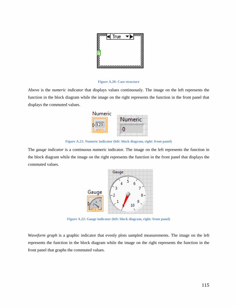
115

Figure A.20: Case structure

Above is the numeric indicator that displays values continuously. The image on the left represents the

function in the block diagram while the image on the right represents the function in the front panel that

displays the commuted values.

Figure A.21: Numeric indicator (left: block diagram, right: front panel)

The gauge indicator is a continuous numeric indicator. The image on the left represents the function in

the block diagram while the image on the right represents the function in the front panel that displays the

commuted values.

Figure A.22: Gauge indicator (left: block diagram, right: front panel)

Waveform graph is a graphic indicator that evenly plots sampled measurements. The image on the left

represents the function in the block diagram while the image on the right represents the function in the

front panel that graphs the commuted values.

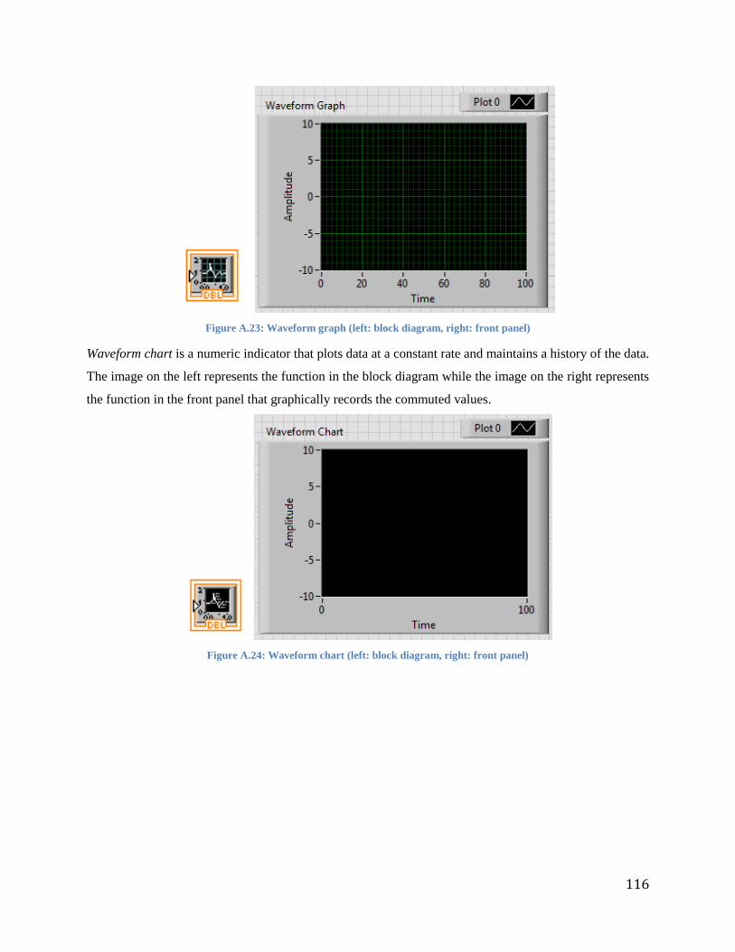
116

Figure A.23: Waveform graph (left: block diagram, right: front panel)

Waveform chart is a numeric indicator that plots data at a constant rate and maintains a history of the data.

The image on the left represents the function in the block diagram while the image on the right represents

the function in the front panel that graphically records the commuted values.

Figure A.24: Waveform chart (left: block diagram, right: front panel)

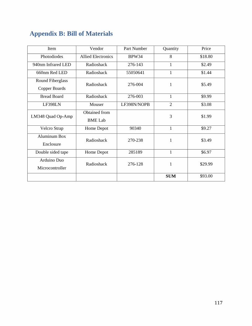
117

Appendix B: Bill of Materials

Item Vendor Part Number Quantity Price

Photodiodes Allied Electronics BPW34 8 $18.80

940nm Infrared LED Radioshack 276-143 1 $2.49

660nm Red LED Radioshack 55050641 1 $1.44

Round Fiberglass

Copper Boards Radioshack 276-004 1 $5.49

Bread Board Radioshack 276-003 1 $9.99

LF398LN Mouser LF398N/NOPB 2 $3.08

LM348 Quad Op-Amp Obtained from

BME Lab 3 $1.99

Velcro Strap Home Depot 90340 1 $9.27

Aluminum Box

Enclosure Radioshack 270-238 1 $3.49

Double sided tape Home Depot 285189 1 $6.97

Arduino Duo

Microcontroller Radioshack 276-128 1 $29.99

SUM $93.00

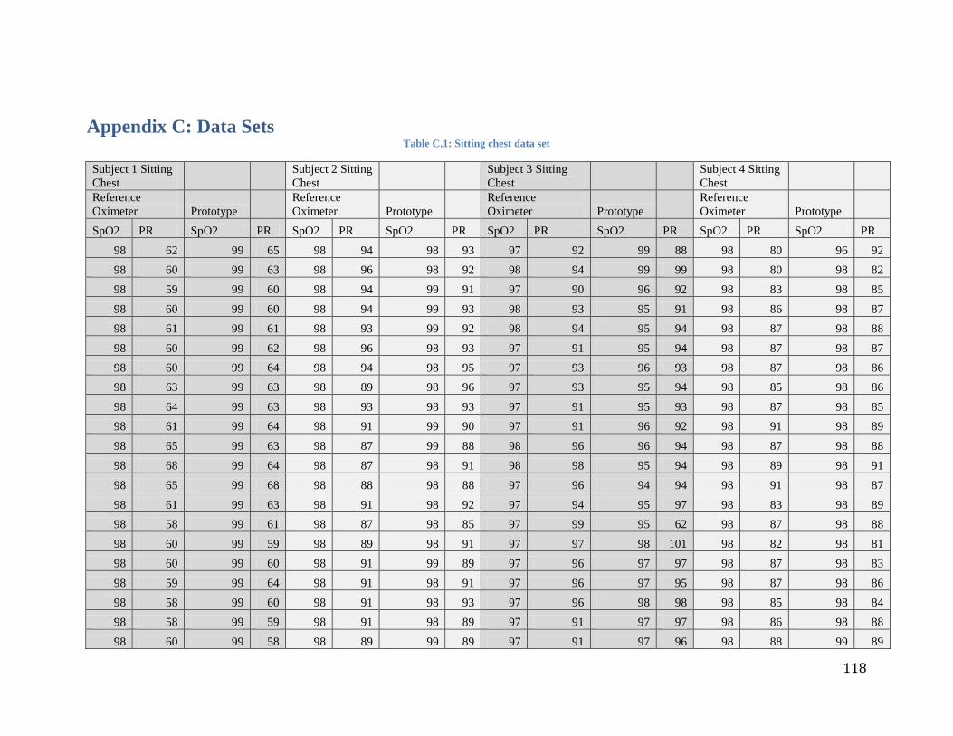
118

Appendix C: Data Sets Table C.1: Sitting chest data set

Subject 1 Sitting

Chest

Subject 2 Sitting

Chest

Subject 3 Sitting

Chest

Subject 4 Sitting

Chest

Reference

Oximeter Prototype

Reference

Oximeter Prototype

Reference

Oximeter Prototype

Reference

Oximeter Prototype

SpO2 PR SpO2 PR SpO2 PR SpO2 PR SpO2 PR SpO2 PR SpO2 PR SpO2 PR

98 62 99 65 98 94 98 93 97 92 99 88 98 80 96 92

98 60 99 63 98 96 98 92 98 94 99 99 98 80 98 82

98 59 99 60 98 94 99 91 97 90 96 92 98 83 98 85

98 60 99 60 98 94 99 93 98 93 95 91 98 86 98 87

98 61 99 61 98 93 99 92 98 94 95 94 98 87 98 88

98 60 99 62 98 96 98 93 97 91 95 94 98 87 98 87

98 60 99 64 98 94 98 95 97 93 96 93 98 87 98 86

98 63 99 63 98 89 98 96 97 93 95 94 98 85 98 86

98 64 99 63 98 93 98 93 97 91 95 93 98 87 98 85

98 61 99 64 98 91 99 90 97 91 96 92 98 91 98 89

98 65 99 63 98 87 99 88 98 96 96 94 98 87 98 88

98 68 99 64 98 87 98 91 98 98 95 94 98 89 98 91

98 65 99 68 98 88 98 88 97 96 94 94 98 91 98 87

98 61 99 63 98 91 98 92 97 94 95 97 98 83 98 89

98 58 99 61 98 87 98 85 97 99 95 62 98 87 98 88

98 60 99 59 98 89 98 91 97 97 98 101 98 82 98 81

98 60 99 60 98 91 99 89 97 96 97 97 98 87 98 83

98 59 99 64 98 91 98 91 97 96 97 95 98 87 98 86

98 58 99 60 98 91 98 93 97 96 98 98 98 85 98 84

98 58 99 59 98 91 98 89 97 91 97 97 98 86 98 88

98 60 99 58 98 89 99 89 97 91 97 96 98 88 99 89

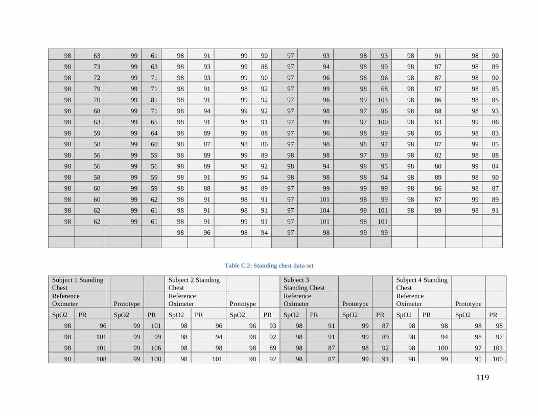
119

98 63 99 61 98 91 99 90 97 93 98 93 98 91 98 90

98 73 99 63 98 93 99 88 97 94 98 99 98 87 98 89

98 72 99 71 98 93 99 90 97 96 98 96 98 87 98 90

98 79 99 71 98 91 98 92 97 99 98 68 98 87 98 85

98 70 99 81 98 91 99 92 97 96 99 103 98 86 98 85

98 68 99 71 98 94 99 92 97 98 97 96 98 88 98 93

98 63 99 65 98 91 98 91 97 99 97 100 98 83 99 86

98 59 99 64 98 89 99 88 97 96 98 99 98 85 98 83

98 58 99 60 98 87 98 86 97 98 98 97 98 87 99 85

98 56 99 59 98 89 99 89 98 98 97 99 98 82 98 88

98 56 99 56 98 89 98 92 98 94 98 95 98 80 99 84

98 58 99 59 98 91 99 94 98 98 98 94 98 89 98 90

98 60 99 59 98 88 98 89 97 99 99 99 98 86 98 87

98 60 99 62 98 91 98 91 97 101 98 99 98 87 99 89

98 62 99 61 98 91 98 91 97 104 99 101 98 89 98 91

98 62 99 61 98 91 99 91 97 101 98 101

98 96 98 94 97 98 99 99

Table C.2: Standing chest data set

Subject 1 Standing

Chest

Subject 2 Standing

Chest

Subject 3

Standing Chest

Subject 4 Standing

Chest

Reference

Oximeter Prototype

Reference

Oximeter Prototype

Reference

Oximeter Prototype

Reference

Oximeter Prototype


98 96 99 101 98 96 96 93 98 91 99 87 98 98 98 98

98 101 99 99 98 94 98 92 98 91 99 89 98 94 98 97

98 101 99 106 98 98 98 89 98 87 98 92 98 100 97 103

98 108 99 108 98 101 98 92 98 87 99 94 98 99 95 100

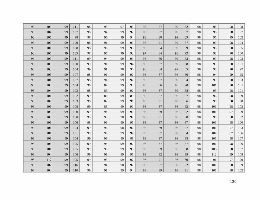
120

98 108 99 111 98 93 97 93 97 87 99 82 98 98 98 98

98 104 99 107 98 94 99 92 98 87 99 87 98 96 98 97

98 106 99 98 98 96 99 94 98 88 99 85 98 96 99 102

98 108 99 109 98 91 99 93 98 91 99 87 98 99 98 104

98 101 99 108 98 96 99 95 98 84 99 89 98 96 98 95

98 106 99 105 98 96 99 93 97 84 98 92 98 98 98 100

98 103 99 111 99 94 99 93 98 86 99 83 98 99 98 103

98 106 99 100 99 91 99 94 98 87 99 88 98 99 98 101

98 103 99 104 99 91 98 90 98 84 99 85 98 98 98 97

98 105 99 107 98 91 99 92 98 87 98 86 98 94 99 95

98 104 99 107 98 91 99 92 98 87 99 84 98 99 98 103

98 103 99 104 98 89 99 93 98 86 98 90 98 101 98 101

98 104 99 103 98 89 99 92 98 87 99 88 98 99 98 101

98 101 99 102 99 88 99 89 98 87 98 87 98 96 98 99

98 104 99 103 98 87 99 91 98 91 98 86 98 98 98 98

98 106 99 108 99 88 99 91 98 87 98 92 98 101 98 103

98 106 99 100 99 94 99 90 98 89 98 92 98 101 97 99

98 108 99 100 99 93 98 92 98 91 98 90 98 98 98 92

98 109 99 106 98 96 99 95 98 87 98 87 98 101 98 100

98 101 99 104 99 96 98 92 98 89 98 87 98 101 97 103

98 101 99 101 99 96 99 94 98 87 99 84 98 104 97 106

98 101 99 104 99 96 99 88 98 87 98 85 98 105 98 107

98 106 99 105 99 94 99 92 98 87 98 87 98 106 98 106

98 101 99 105 99 93 99 98 98 89 98 88 98 106 98 107

98 104 99 106 99 91 99 95 98 92 98 89 98 112 99 108

98 112 99 105 99 93 99 92 98 91 98 89 98 96 97 99

98 107 99 116 99 94 98 92 98 87 98 92 98 101 98 99

98 104 99 110 99 91 99 94 98 89 98 91 98 101 98 102

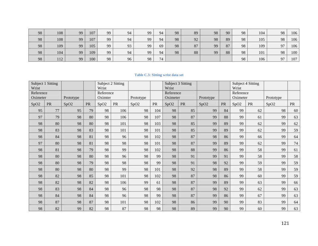
121

98 108 99 107 99 94 99 94 98 89 98 90 98 104 98 106

98 108 99 107 99 94 99 94 98 92 98 89 98 105 98 106

98 109 99 105 99 93 99 69 98 87 99 87 98 109 97 106

98 104 99 109 99 94 99 94 98 88 99 88 98 101 98 100

98 112 99 100 98 96 98 74

98 106 97 107

Table C.3: Sitting wrist data set

Subject 1 Sitting

Wrist

Subject 2 Sitting

Wrist

Subject 3 Sitting

Wrist

Subject 4 Sitting

Wrist

Reference

Oximeter Prototype

Reference

Oximter Prototype

Reference

Oximeter Prototype

Reference

Oximeter Prototype


95 77 95 79 98 106 98 104 98 85 99 84 99 62 98 60

97 79 98 80 98 106 98 107 98 87 99 88 99 61 99 63

98 80 98 80 98 101 98 103 98 85 99 89 99 62 99 62

98 83 98 83 98 101 98 101 98 85 99 89 99 62 99 59

98 84 98 81 98 96 98 102 98 87 98 86 99 66 99 64

97 80 98 81 98 98 98 101 98 87 99 89 99 62 99 74

98 81 98 79 98 99 98 102 98 88 99 86 99 58 99 61

98 80 98 80 98 96 98 99 98 91 99 91 99 58 99 58

98 80 98 79 98 98 98 99 98 91 98 92 99 59 99 59

98 80 98 80 98 99 98 101 98 92 98 89 99 58 99 59

98 82 98 85 98 101 98 102 98 87 98 86 99 60 99 59

98 82 98 82 98 106 99 61 98 87 99 89 99 63 99 66

98 83 98 84 98 96 98 98 98 87 98 92 99 62 99 63

98 84 98 84 98 96 98 99 98 87 99 86 99 67 99 63

98 87 98 87 98 101 98 102 98 86 99 90 99 83 99 64

98 82 99 82 98 87 98 98 98 89 99 90 99 60 99 63

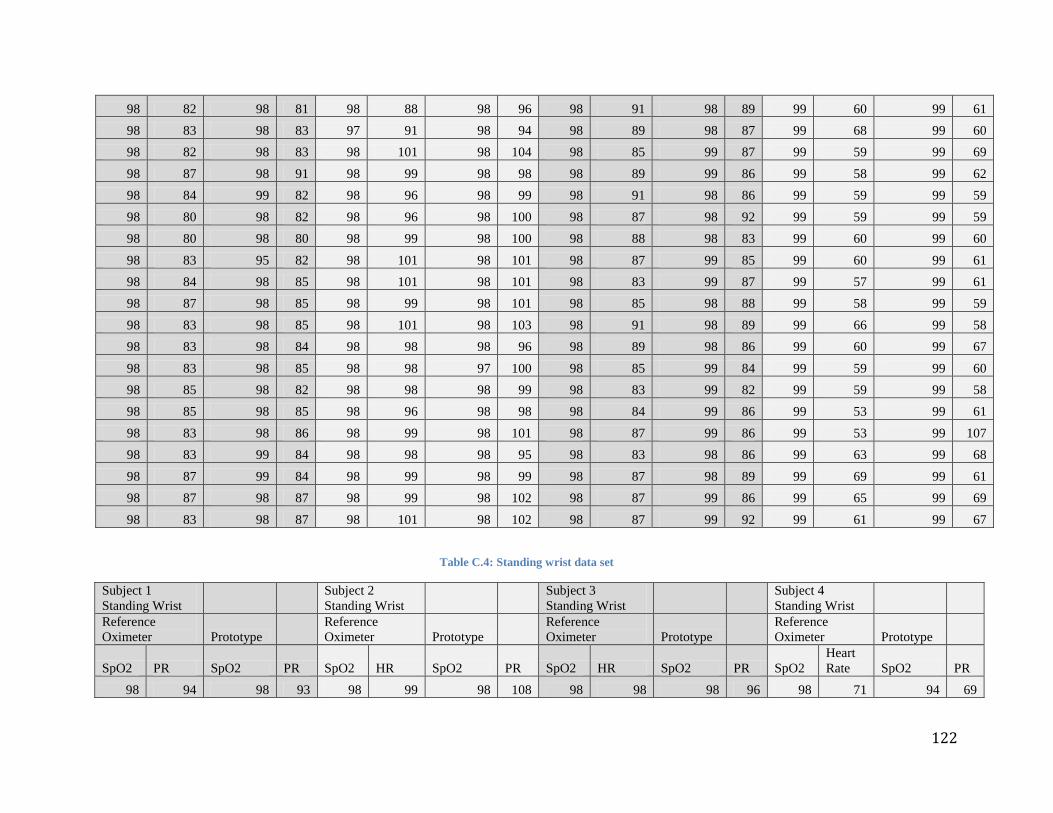
122

98 82 98 81 98 88 98 96 98 91 98 89 99 60 99 61

98 83 98 83 97 91 98 94 98 89 98 87 99 68 99 60

98 82 98 83 98 101 98 104 98 85 99 87 99 59 99 69

98 87 98 91 98 99 98 98 98 89 99 86 99 58 99 62

98 84 99 82 98 96 98 99 98 91 98 86 99 59 99 59

98 80 98 82 98 96 98 100 98 87 98 92 99 59 99 59

98 80 98 80 98 99 98 100 98 88 98 83 99 60 99 60

98 83 95 82 98 101 98 101 98 87 99 85 99 60 99 61

98 84 98 85 98 101 98 101 98 83 99 87 99 57 99 61

98 87 98 85 98 99 98 101 98 85 98 88 99 58 99 59

98 83 98 85 98 101 98 103 98 91 98 89 99 66 99 58

98 83 98 84 98 98 98 96 98 89 98 86 99 60 99 67

98 83 98 85 98 98 97 100 98 85 99 84 99 59 99 60

98 85 98 82 98 98 98 99 98 83 99 82 99 59 99 58

98 85 98 85 98 96 98 98 98 84 99 86 99 53 99 61

98 83 98 86 98 99 98 101 98 87 99 86 99 53 99 107

98 83 99 84 98 98 98 95 98 83 98 86 99 63 99 68

98 87 99 84 98 99 98 99 98 87 98 89 99 69 99 61

98 87 98 87 98 99 98 102 98 87 99 86 99 65 99 69

98 83 98 87 98 101 98 102 98 87 99 92 99 61 99 67

Table C.4: Standing wrist data set

Subject 1

Standing Wrist

Subject 2

Standing Wrist

Subject 3

Standing Wrist

Subject 4

Standing Wrist

Reference

Oximeter Prototype

Reference

Oximeter Prototype

Reference

Oximeter Prototype

Reference

Oximeter Prototype

SpO2 PR SpO2 PR SpO2 HR SpO2 PR SpO2 HR SpO2 PR SpO2

Heart

Rate SpO2 PR

98 94 98 93 98 99 98 108 98 98 98 96 98 71 94 69

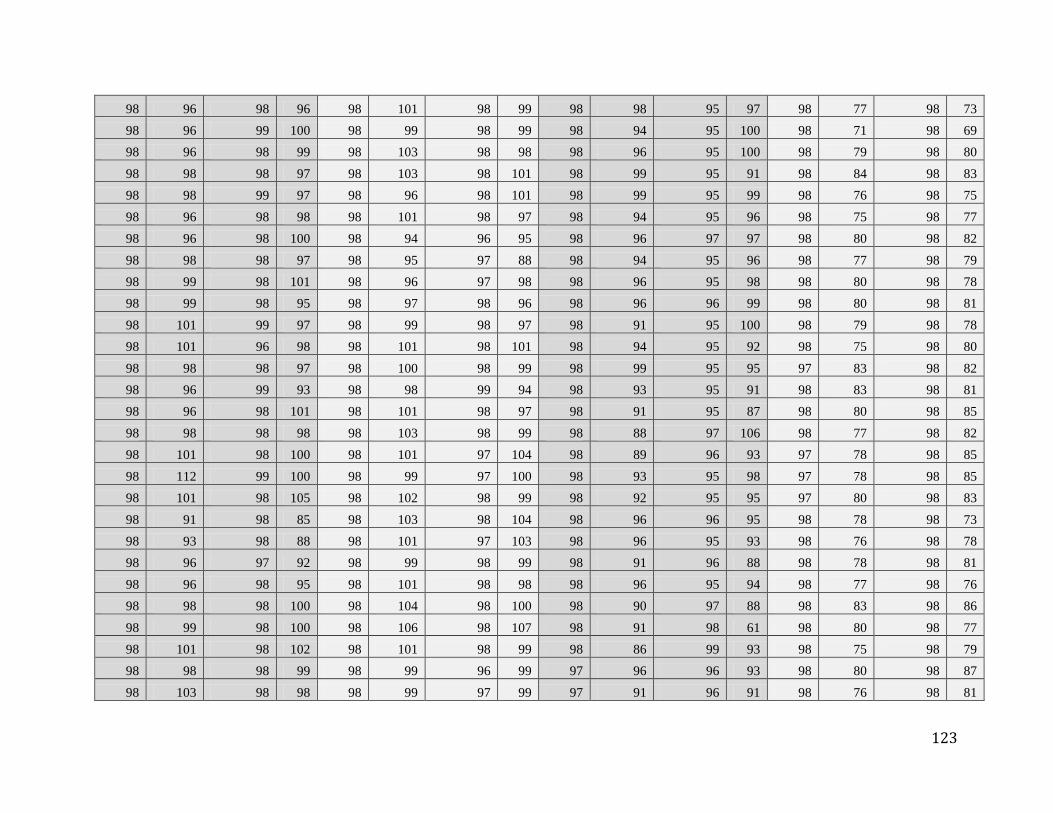
123

98 96 98 96 98 101 98 99 98 98 95 97 98 77 98 73

98 96 99 100 98 99 98 99 98 94 95 100 98 71 98 69

98 96 98 99 98 103 98 98 98 96 95 100 98 79 98 80

98 98 98 97 98 103 98 101 98 99 95 91 98 84 98 83

98 98 99 97 98 96 98 101 98 99 95 99 98 76 98 75

98 96 98 98 98 101 98 97 98 94 95 96 98 75 98 77

98 96 98 100 98 94 96 95 98 96 97 97 98 80 98 82

98 98 98 97 98 95 97 88 98 94 95 96 98 77 98 79

98 99 98 101 98 96 97 98 98 96 95 98 98 80 98 78

98 99 98 95 98 97 98 96 98 96 96 99 98 80 98 81

98 101 99 97 98 99 98 97 98 91 95 100 98 79 98 78

98 101 96 98 98 101 98 101 98 94 95 92 98 75 98 80

98 98 98 97 98 100 98 99 98 99 95 95 97 83 98 82

98 96 99 93 98 98 99 94 98 93 95 91 98 83 98 81

98 96 98 101 98 101 98 97 98 91 95 87 98 80 98 85

98 98 98 98 98 103 98 99 98 88 97 106 98 77 98 82

98 101 98 100 98 101 97 104 98 89 96 93 97 78 98 85

98 112 99 100 98 99 97 100 98 93 95 98 97 78 98 85

98 101 98 105 98 102 98 99 98 92 95 95 97 80 98 83

98 91 98 85 98 103 98 104 98 96 96 95 98 78 98 73

98 93 98 88 98 101 97 103 98 96 95 93 98 76 98 78

98 96 97 92 98 99 98 99 98 91 96 88 98 78 98 81

98 96 98 95 98 101 98 98 98 96 95 94 98 77 98 76

98 98 98 100 98 104 98 100 98 90 97 88 98 83 98 86

98 99 98 100 98 106 98 107 98 91 98 61 98 80 98 77

98 101 98 102 98 101 98 99 98 86 99 93 98 75 98 79

98 98 98 99 98 99 96 99 97 96 96 93 98 80 98 87

98 103 98 98 98 99 97 99 97 91 96 91 98 76 98 81

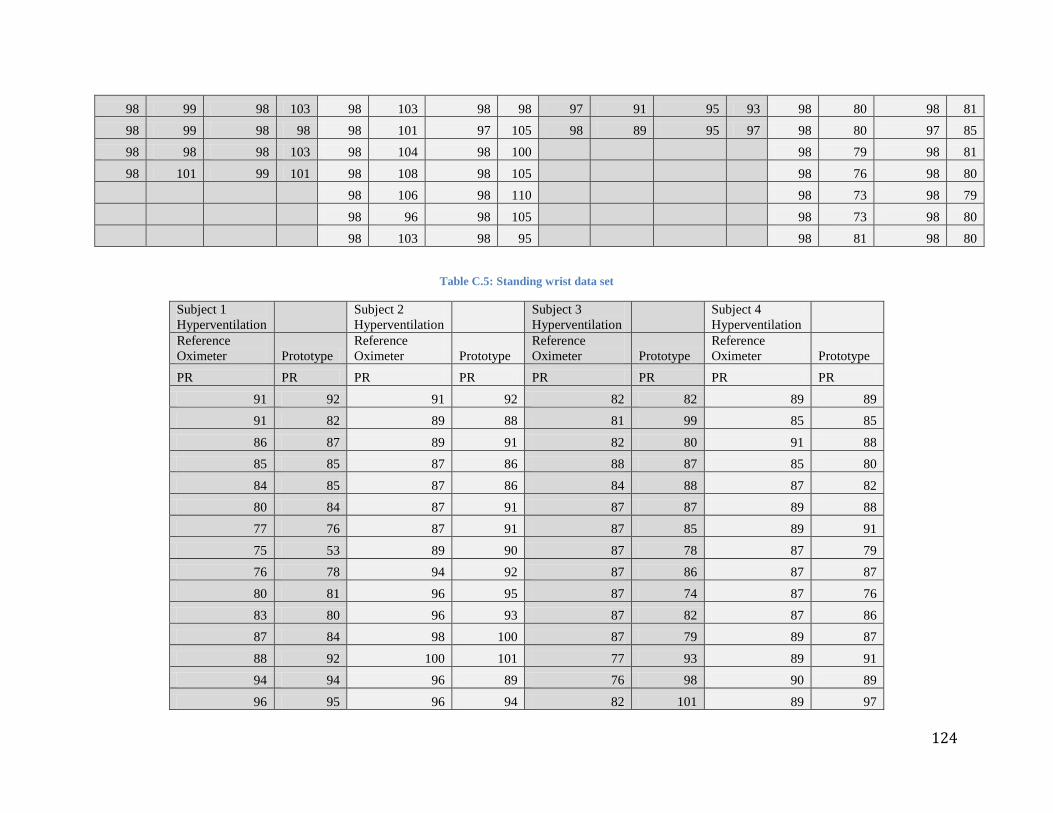
124

98 99 98 103 98 103 98 98 97 91 95 93 98 80 98 81

98 99 98 98 98 101 97 105 98 89 95 97 98 80 97 85

98 98 98 103 98 104 98 100

98 79 98 81

98 101 99 101 98 108 98 105

98 76 98 80

98 106 98 110

98 73 98 79

98 96 98 105

98 73 98 80

98 103 98 95

98 81 98 80

Table C.5: Standing wrist data set

Subject 1

Hyperventilation

Subject 2

Hyperventilation

Subject 3

Hyperventilation

Subject 4

Hyperventilation

Reference

Oximeter Prototype

Reference

Oximeter Prototype

Reference

Oximeter Prototype

Reference

Oximeter Prototype

PR PR PR PR PR PR PR PR

91 92 91 92 82 82 89 89

91 82 89 88 81 99 85 85

86 87 89 91 82 80 91 88

85 85 87 86 88 87 85 80

84 85 87 86 84 88 87 82

80 84 87 91 87 87 89 88

77 76 87 91 87 85 89 91

75 53 89 90 87 78 87 79

76 78 94 92 87 86 87 87

80 81 96 95 87 74 87 76

83 80 96 93 87 82 87 86

87 84 98 100 87 79 89 87

88 92 100 101 77 93 89 91

94 94 96 89 76 98 90 89

96 95 96 94 82 101 89 97

125

99 101 96 92 96 111 89 90

101 100 91 95 99 110 87 91

103 105 91 88 106 110 98 101

103 104 87 95 108 107 101 94

101 102 87 81 108 113 101 99

101 91 92 93 106 115 101 95

98 99 95 91 109 115 106 105

99 94 96 97 112 118 110 110

96 94 96 95 112 121 116 119

96 100 98 95 115 111 120 113

91 96 98 91 117 109 124 80

87 91 99 90 113 97 128 126

86 85 104 97 108 91 112 134

87 86 104 103 103 90 112 131

87 88 103 109 93 91 108 115

87 88 101 108 91 92 106 109

87 87 101 97 89 97 101 101

87 89 91 95 91 84 99 99

87 86 90 100 92 89

87 87 96 86 89 68

Table C.6: Hyperventilation data set

Subject 1

Subject 2

Reference Oximeter Prototype Reference Oximeter Prototype

SpO2 SpO2 SpO2 SpO2

99 97 98 98

99 97 98 98

99 98 98 98

126

99 97 98 97

99 97 98 98

99 97 98 98

99 97 98 98

99 98 98 96

99 97 98 98

99 97 98 97

99 97 97 96

99 97 97 98

99 96 97 98

99 97 98 99

99 97 98 99

99 98 93 99

99 97 97 93

99 98 97 99

99 97 98 94

99 98 98 98

99 98 98 97

99 97 99 98

99 97 95 98

99 97 97 96

97 96 98 99

97 96 98 98

96 95 98 99

94 95 98 98

92 94 97 98

91 93 97 98

94 96 96 98

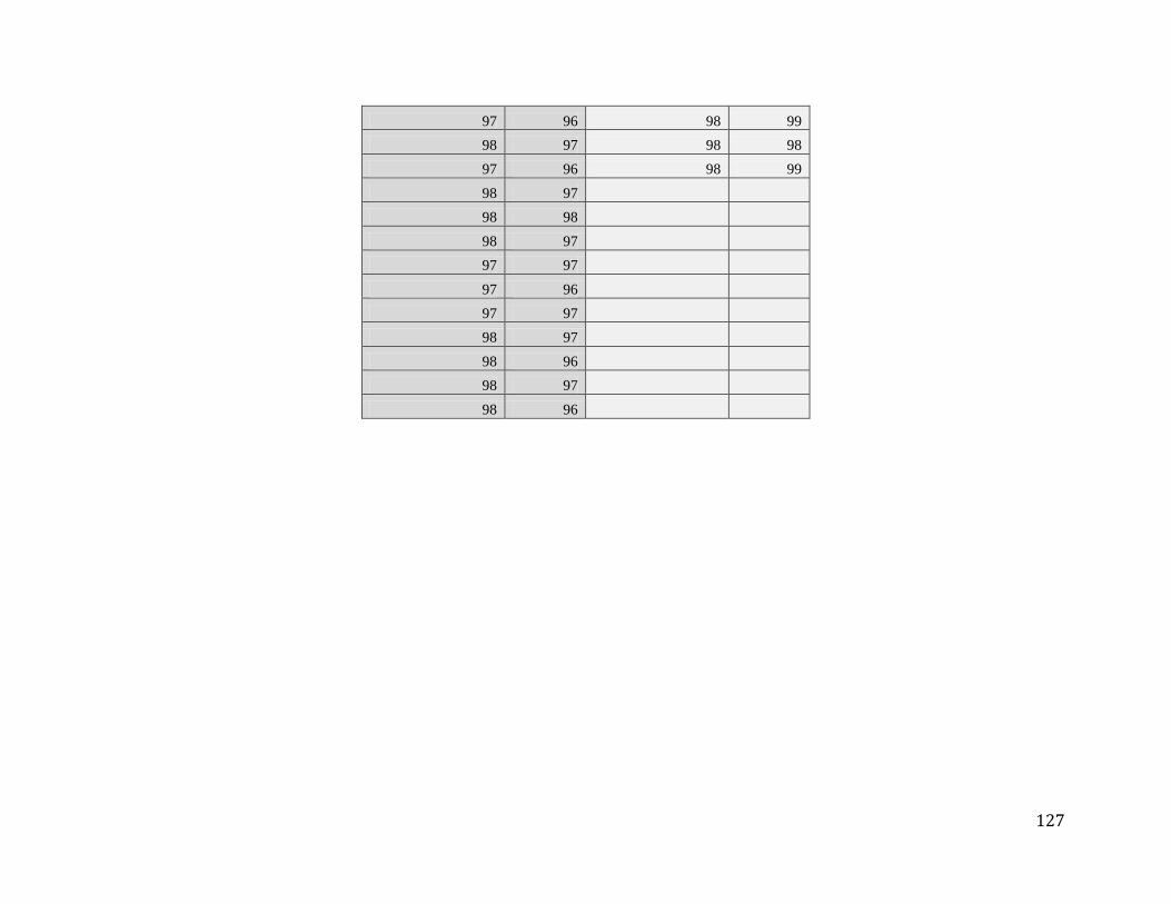
127

97 96 98 99

98 97 98 98

97 96 98 99

98 97

98 98

98 97

97 97

97 96

97 97

98 97

98 96

98 97

98 96

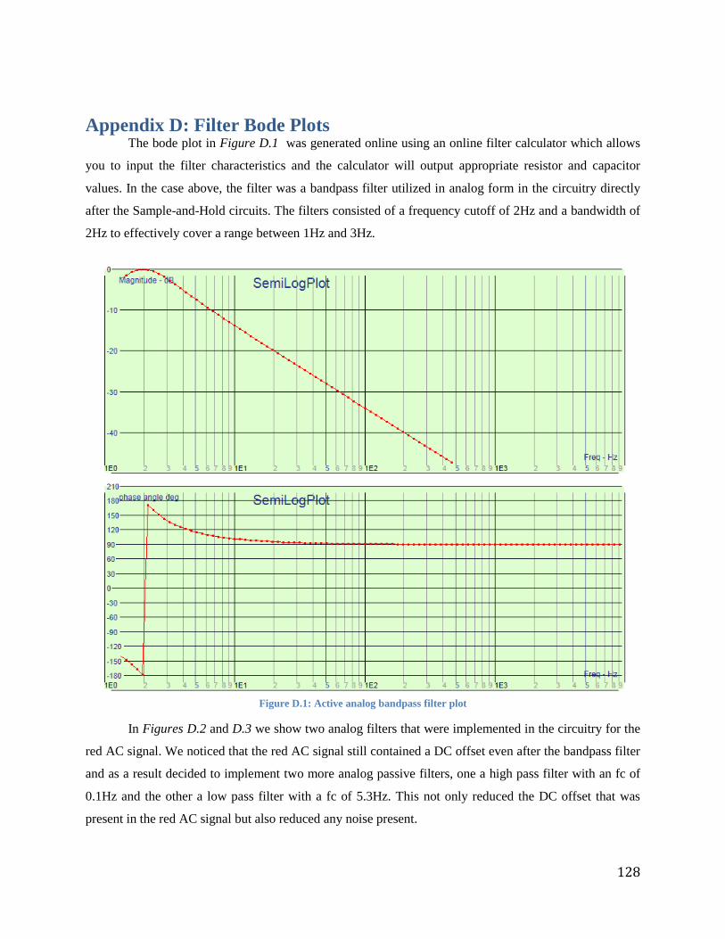
128

Appendix D: Filter Bode Plots The bode plot in Figure D.1 was generated online using an online filter calculator which allows

you to input the filter characteristics and the calculator will output appropriate resistor and capacitor

values. In the case above, the filter was a bandpass filter utilized in analog form in the circuitry directly

after the Sample-and-Hold circuits. The filters consisted of a frequency cutoff of 2Hz and a bandwidth of

2Hz to effectively cover a range between 1Hz and 3Hz.

Figure D.1: Active analog bandpass filter plot

In Figures D.2 and D.3 we show two analog filters that were implemented in the circuitry for the

red AC signal. We noticed that the red AC signal still contained a DC offset even after the bandpass filter

and as a result decided to implement two more analog passive filters, one a high pass filter with an fc of

0.1Hz and the other a low pass filter with a fc of 5.3Hz. This not only reduced the DC offset that was

present in the red AC signal but also reduced any noise present.

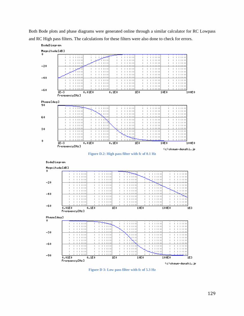
129

Both Bode plots and phase diagrams were generated online through a similar calculator for RC Lowpass

and RC High pass filters. The calculations for these filters were also done to check for errors.

Figure D.2: High pass filter with fc of 0.1 Hz

Figure D 3: Low pass filter with fc of 5.3 Hz

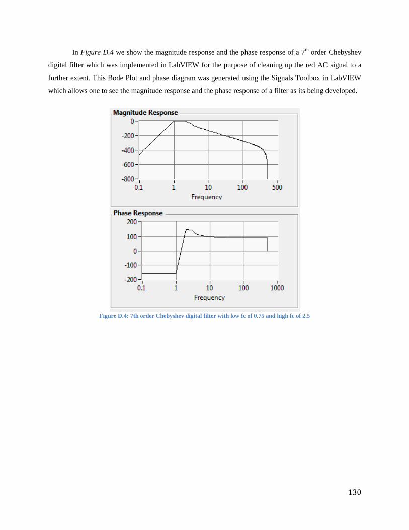
130

In Figure D.4 we show the magnitude response and the phase response of a 7th order Chebyshev

digital filter which was implemented in LabVIEW for the purpose of cleaning up the red AC signal to a

further extent. This Bode Plot and phase diagram was generated using the Signals Toolbox in LabVIEW

which allows one to see the magnitude response and the phase response of a filter as its being developed.

Figure D.4: 7th order Chebyshev digital filter with low fc of 0.75 and high fc of 2.5

Documents

REFLECTANCE-BASED PULSE OXIMETER FOR THE … · In this project, a reflectance-based pulse oximeter was ... which transmittance based pulse oximetry cannot ... components and a programmed