ref28

7/29/2019 ref28

http://slidepdf.com/reader/full/ref28 1/6

Enhanced Robot Audition Based on Microphone

Array Source Separation with Post-Filter

Jean-Marc Valin, Jean Rouat, François Michaud

LABORIUS – Research Laboratory on Mobile Robotics and Intelligent Systems

Department of Electrical Engineering and Computer Engineering

Université de Sherbrooke, Sherbrooke (Quebec) CANADA, J1K 2R1

{Jean-Marc.Valin, Jean.Rouat, Francois.Michaud}@USherbrooke.ca

Abstract— We propose a system that gives a mobile robotthe ability to separate simultaneous sound sources. A mi-crophone array is used along with a real-time dedicatedimplementation of Geometric Source Separation and a post-filter that gives us a further reduction of interferences fromother sources. We present results and comparisons for sep-aration of multiple non-stationary speech sources combined

with noise sources. The main advantage of our approach formobile robots resides in the fact that both the frequency-domain Geometric Source Separation algorithm and thepost-filter are able to adapt rapidly to new sources andnon-stationarity. Separation results are presented for threesimultaneous interfering speakers in the presence of noise.A reduction of log spectral distortion (LSD) and increase of signal-to-noise ratio (SNR) of approximately 10 dB and 14 dBare observed.

I. INTRODUCTION

Our hearing sense allows us to perceive all kinds of

sounds (speech, music, phone ring, closing a door, etc.)

in our world, whether we are moving or not. To operate

in human and natural settings, autonomous mobile robots

should be able to do the same. This requires the robots

not just to detect sounds, but also to localise their origin,

separate the different sound sources (since sounds may

occur simultaneously), and process all of this data to extract

useful information about the world.

Even though artificial hearing would be an important

sensing capability for autonomous systems, the research

topic is still in its infancy. Only a few robots are using

hearing capabilities: SAIL [1] uses one microphone to

develop online audio-driven behaviors; ROBITA [2] uses

two microphones to follow a conversation between two

persons; SIG [3], [4], [5] uses one pair of microphonesto collect sound from the external world, and another pair

placed inside the head to collect internal sounds (caused

by motors) for noise cancellation; Sony SDR-4X has

seven microphones; a service robot uses eight microphones

organised in a circular array to do speech enhancement and

recognition [6]. Even though robots are not limited to only

two ears, they still have not shown the capabilities of the

human hearing sense.

We address the problem of isolating sound sources

from the environment. The human hearing sense is very

good at focusing on a single source of interest despite all

kinds of interferences. We generally refer to this ability asthe cocktail party effect , where a human listener is able

Fig. 1. Overview of the separation system

to follow a conversation even when several people are

speaking at the same time. For a mobile robot, it would

mean being able to separate all sound sources present in

the environment at any moment.

Working toward that goal, our interest in this paper is to

describe a two-step approach for performing sound source

separation on a mobile robot equipped with an array of

eight low-cost microphones. The initial step consists of

a linear separation based on a simplified version of theGeometric Source Separation approach proposed by Parra

and Alvino [7] with a faster stochastic gradient estimation

and shorter time frames estimations. The second step is

a generalisation of beamformer post-filtering [8], [9] for

multiple sources and uses adaptive spectral estimation of

background noise and interfering sources to enhance the

signal produced during the initial separation. The novelty

of this post-filter resides in the fact that, for each source of

interest, the noise estimate is decomposed into stationary

and transient components assumed to be due to leakage

between the output channels of the initial separation stage.

The paper is organised as follows. Section II gives an

overview of the system. Section III presents the linear

separation algorithm and Section IV describes the proposed

post-filter. Results are presented in Section V, followed by

the conclusion.

II. SYSTEM OVERVIEW

The proposed sound separation algorithm as shown in

Figure 1 is composed of three parts:

1) A microphone array;

2) A linear source separation algorithm (LSS) imple-

mented as a variant of the Geometric Source Sepa-

ration (GSS) algorithm;3) A multi-channel post-filter.

7/29/2019 ref28


The microphone array is composed of a number of

omni-directional elements mounted on the robot. The

microphone signals are combined linearly in a first-pass

separation algorithm. The output of this initial separation

is then enhanced by a (non-linear) post-filter designed to

optimally attenuate the remaining noise and interference

from other sources.

We assume that these sources are detected and localised

by an algorithm such as [10] (our approach is not specific

to any localisation algorithm). We also assume that sources

may appear, disappear or move at any time. It is thus

necessary to maximise the adaptation rate for both the

LSS and the multi-channel post-filter. Mobile robotics also

imposes real-time constraints: the algorithmic delay must

be kept small and the complexity must be low enough for

the algorithm to process data in real-time on a conventional

processor.

III. LINEAR SOURCE SEPARATION

The LSS algorithm we propose in this section is based on

the Geometric Source Separation (GSS) approach proposed

by Parra and Alvino [7]. Unlike the Linearly Constrained

Minimum Variance (LCMV) beamformer that minimises

the output power subject to a distortionless constraint, GSS

explicitly minimises cross-talk, leading to faster adaptation.

The method is also interesting for use in the mobile

robotics context because it allows easy addition and re-

moval of sources. Using some approximations described in

Subsection III-B, it is also possible to implement separation

with relatively low complexity (i.e. complexity that grows

linearly with the number of microphones).

A. Geometric Source Separation

The method operates in the frequency domain. Let

S m(k, ) be the real (unknown) sound source m at time

frame and for discrete frequency k. We denote as s(k, )the vector corresponding to the sources S m(k, ) and ma-

trix A(k) is the transfer function leading from the sources

to the microphones. The signal received at the microphones

is thus given by:

x(k, ) = A(k)s(k, ) + n(k, ) (1)

where n(k, ) is the non-coherent background noise re-

ceived at the microphones. The matrix A(k) can be esti-

mated using the result of a sound localisation algorithm.

Assuming that all transfer functions have unity gain, theelements of A(k) can be expressed as:

aij(k) = e−2πkδij (2)

where δ ij is the time delay (in samples) to reach micro-

phone i from source j.

The separation result is then defined as y(k, ) =W(k, )x(k, ), where W(k, ) is the separation matrix

that must be estimated. This is done by providing two

constraints (the index is omitted for the sake of clarity):

1) Decorrelation of the separation algorithm outputs,

expressed as Ryy(k) − diag [Ryy(k)] = 01.

1Assuming non-stationary sources, second order statistics are sufficientfor ensuring independence of the separated sources.

2) The geometric constraint W(k)A(k) = I, which

ensures unity gain in the direction of the source of

interest and places zeros in the direction of interfer-

ences.

In theory, constraint 2) could be used alone for separation

(the method is referred to as LS-C2 in [7]), but in practice,

the method does not take into account reverberation or er-rors in localisation. It is also subject to instability if A(k) is

not invertible at a specific frequency. When used together,

constraints 1) and 2) are too strong. For this reason, we

propose “soft” constraints that are a combination of 1) and

2) in the context of a gradient descent algorithm.

Two cost functions are created by computing the square

of the error associated with constraints 1) and 2). These

cost functions are respectively defined as:

J 1(W(k)) = Ryy(k) − diag [Ryy(k)]2 (3)

J 2(W(k)) = W(k)A(k) − I2 (4)

where the matrix norm is defined as M

2

=traceMMH

and is equal to the sum of the square of all

elements in the matrix. The gradient of the cost functions

with respect to W(k) is equal to [7]:

∂J 1(W(k))

∂ W∗(k)= 4E(k)W(k)Rxx(k) (5)

∂J 2(W(k))

∂ W∗(k)= 2 [W(k)A(k) − I]A(k) (6)

where E(k) = Ryy(k) − diag [Ryy(k)].

The separation matrix W(k) is then updated as follows:

Wn+1(k) = Wn(k)−µα(k)∂J 1(W(k))

∂ W∗(k)+

∂J 2(W(k))

∂ W∗(k)

(7)

where α(f ) is an energy normalisation factor equal to

Rxx(k)−2

and µ is the adaptation rate.

B. Stochastic Gradient Adaptation

The difference between our algorithm and the original

GSS algorithm described in [7] is that instead of estimating

the correlation matrices Rxx(k) and Ryy(k) on several

seconds of data, our approach uses instantaneous estima-

tions. This is analogous to the approximation made in the

Least Mean Square (LMS) adaptive filter [11]. We thus

assume that:

Rxx(k) = x(k)x(k)H (8)

Ryy(k) = y(k)y(k)H (9)

It is then possible to rewrite the gradient∂J 1(W(k))∂ W∗(k)

as:

∂J 1(W(k))

∂ W∗(k)= 4 [E(k)W(k)x(k)]x(k)H (10)

which only requires matrix-by-vector products, greatly re-

ducing the complexity of the algorithm. The normalisation

factor α(k) can also be simplified as

x(k)2−2

. From

this work, the instantaneous estimation of the correlation

has not shown any reduction in accuracy and furthermoreeases real-time integration.

7/29/2019 ref28


Geometricsource

separation

Attenuationrule

Y m(k,l)

Stationarynoise

estimation

Interferenceleak

estimation

SNR & speechprobatilityestimation

+

S m(k,l) X n(k,l)

λmstat.(k ,l)

λmleak (k ,l)

^

λm(k ,l)

Fig. 2. Overview of the post-filter.X n(k, ), n = 0 . . . N − 1: Microphone inputs,Y m(k, ), m = 0 . . . M − 1: Inputs to the post-filter,

S m(k, ) = Gm(k, )Y m(k, ), m = 0 . . . M − 1: Post-filteroutputs.

C. Initialisation

The fact that sources can appear or disappear at any timeimposes constraints on the initialisation of the separation

matrix W(k). The initialisation must provide the follow-

ing:

• The initial weights for a new source;

• Acceptable separation (before adaptation).

Furthermore, when a source appears or disappears, other

sources must be unaffected.

One easy way to satisfy both constraints is to initialise

the column of W(k) corresponding to the new source mas:

wm,i(k) =ai,m(k)

N

(11)

This initialisation is equivalent to a delay-and-sum

beamformer, and is referred to as the I1 initialisation

method in [7].

IV. MULTI-CHANNEL POST-FILTER

In order to enhance the output of the GSS algorithm

presented in Section III, we derive a frequency-domain

post-filter that is based on the optimal estimator origi-

nally proposed by Ephraim and Malah [12], [13]. Several

approaches to microphone array post-filtering have been

proposed in the past. Most of these post-filters address

reduction of stationary background noise [14], [15]. Re-cently, a multi-channel post-filter taking into account non-

stationary interferences was proposed by Cohen [8]. The

novelty of our approach resides in the fact that, for a given

channel output of the GSS, the transient components of the

corrupting sources is assumed to be due to leakage from the

other channels during the GSS process. Furthermore, for a

given channel, the stationary and the transient components

are combined into a single noise estimator used for noise

suppression, as shown in Figure 2.

For this post-filter, we consider that all interferences

(except the background noise) are localised (detected by

the localisation algorithm) sources and we assume thatthe leakage between channels is constant. This leakage

is due to reverberation, localisation error, differences in

microphone frequency responses, near-field effects, etc.

Section IV-A describes the estimation of noise variances

that are used to compute the weighting function Gm by

which the outputs Y m of the LSS is multiplied to generate

a cleaned signal whose spectrum is denoted S m.

A. Noise estimation

The noise variance estimation λm(k, ) is expressed as:

λm(k, ) = λstat.m (k, ) + λleak

m (k, ) (12)

where λstat.m (k, ) is the estimate of the stationary compo-

nent of the noise for source m at frame for frequency k,

and λleakm (k, ) is the estimate of source leakage.

We compute the stationary noise estimate λstat.m (k, )

using the Minima Controlled Recursive Average (MCRA)

technique proposed by Cohen [16].

To estimate λleakm we assume that the interference from

other sources is reduced by a factor η (typically −10dB ≤

η ≤ −5dB) by the separation algorithm (LSS). The leakageestimate is thus expressed as:

λleakm (k, ) = η

M −1i=0,i=m

Z i(k, ) (13)

where Z m(k, ) is the smoothed spectrum of the mth

source, Y m(k, ), and is recursively defined (with αs = 0.7)

as:

Z m(k, ) = αsZ m(k, − 1) + (1 − αs)Y m(k, ) (14)

B. Suppression rule in the presence of speech

We now derive the suppression rule under H 1, thehypothesis that speech is present. From here on, unless

otherwise stated, the m index and the arguments are

omitted for clarity and the equations are given for each

m and for each .

The proposed noise suppression rule is based on mini-

mum mean-square error (MMSE) estimation of the spectral

amplitude in the loudness domain, |X (k)|1/2

. The choice

of the loudness domain over the spectral amplitude [12] or

log-spectral amplitude [13] is motivated by better results

obtained using this technique, mostly when dealing with

speech presence uncertainty (Section IV-C).

The loudness-domain amplitude estimator is defined by:

A(k) = (E [|S (k)|α

|Y (k) ])1

α = GH 1(k) |Y (k)| (15)

where α = 1/2 for the loudness domain and GH 1(k) is

the spectral gain assuming that speech is present.

The spectral gain for arbitrary α is derived from Equa-

tion 13 in [13]:

GH 1(k) =

υ(k)

γ (k)

Γ

1 +α

2

M

−α

2; 1; −υ(k)

1

α

(16)

where M (a; c; x) is the confluent hypergeometric function,

γ (k) |Y (k)|2 /λ(k) and ξ (k) E

|S (k)|2/λ(k) are

respectively the a posteriori SNR and the a priori SNR.We also have υ(k) γ (k)ξ (k)/ (ξ (k) + 1) [12].

7/29/2019 ref28


The a priori SNR ξ (k) is estimated recursively as:

ξ (k, l) = α pG2H 1(k, − 1)γ (k, − 1)

+ (1 − α p)max {γ (k, ) − 1, 0} (17)

using the modifications proposed in [16] to take into

account speech presence uncertainty.

C. Optimal gain modification under speech presence un-

certainty

In order to take into account the probability of speech

presence, we derive the estimator for the loudness domain:

A(k) = (E [Aα(k)| Y (k)])1

α (18)

Considering H 1, the hypothesis of speech presence for

source m, and H 0, the hypothesis of speech absence, we

obtain:

E [Aα(k)|Y (k)] = p(k)E [Aα(k)|H 1, Y (k)]

+ [1− p(k)]E [Aα(k)|H 0,Y (k)](19)

where p(k) is the probability of speech at frequency k.

The optimally modified gain is thus given by:

G(k) = p(k)Gα

H 1(k) + (1 − p(k))Gαmin

1α (20)

where GH 1(k) is defined in (16), and Gmin is the minimum

gain allowed when speech is absent. Unlike the log-

amplitude case, it is possible to set Gmin = 0 without

running into problems. For α = 1/2, this leads to:

G(k) = p2(k)GH 1(k) (21)

Setting Gmin = 0 means that there is no arbitrary limit

on attenuation. Therefore, when the signal is certain tobe non-speech, the gain can tend toward zero. This is

especially important when the interference is also speech

since, unlike stationary noise, residual babble noise always

results in musical noise.

The probability of speech presence is computed as:

p(k) =

1 +

q (k)

1 − q (k)(1 + ξ (k))exp(−υ(k))

−1(22)

where q (k) is the a priori probability of speech presence

for frequency k and is defined as:

q (k) = 1 − P local(k)P global(k)P frame (23)

where P local(k), P global(k) and P frame are defined in [16]

and correspond respectively to a speech measurement on

the current frame for a local frequency window, a larger

frequency and for the whole frame.

D. Initialisation

When a new source appears, post-filter state variables

need to be initialised. Most of these variables may safely

be set to zero. The exception is λstat.m (k, 0), the initial

stationary noise estimation for source m. The MCRA

algorithm requires several seconds to produce its first

estimate for source m, so it is necessary to find another way

to estimate the background noise until a better estimate isavailable. This initial estimate is thus computed using noise

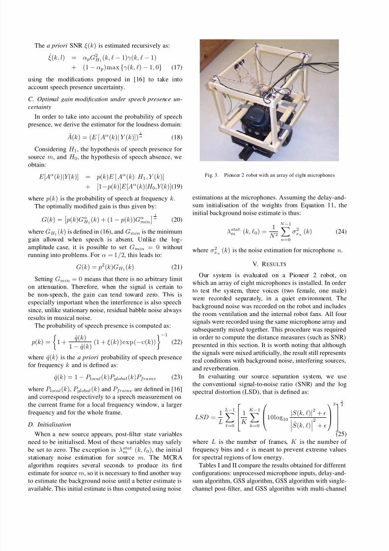
Fig. 3. Pioneer 2 robot with an array of eight microphones

estimations at the microphones. Assuming the delay-and-

sum initialisation of the weights from Equation 11, the

initial background noise estimate is thus:

λstat.m (k, 0) =

1

N 2

N −1n=0

σ2xn (k) (24)

where σ2xn (k) is the noise estimation for microphone n.

V. RESULTS

Our system is evaluated on a Pioneer 2 robot, on

which an array of eight microphones is installed. In order

to test the system, three voices (two female, one male)were recorded separately, in a quiet environment. The

background noise was recorded on the robot and includes

the room ventilation and the internal robot fans. All four

signals were recorded using the same microphone array and

subsequently mixed together. This procedure was required

in order to compute the distance measures (such as SNR)

presented in this section. It is worth noting that although

the signals were mixed artificially, the result still represents

real conditions with background noise, interfering sources,

and reverberation.

In evaluating our source separation system, we use

the conventional signal-to-noise ratio (SNR) and the logspectral distortion (LSD), that is defined as:

LSD =1

L

L−1=0

1

K

K −1k=0

10log10

|S (k, )|2 + S (k, )2 +

2

1

2

(25)

where L is the number of frames, K is the number of

frequency bins and is meant to prevent extreme values

for spectral regions of low energy.

Tables I and II compare the results obtained for different

configurations: unprocessed microphone inputs, delay-and-

sum algorithm, GSS algorithm, GSS algorithm with single-channel post-filter, and GSS algorithm with multi-channel

7/29/2019 ref28


TABLE I

SIGNAL-TO-NOISE RATIO (SNR) FOR EACH OF THE THREE

SEPARATED SOURCES.

SNR (dB) female 1 female 2 male 1

Microphone inputs -1.8 -3.7 -5.2

Delay-and-sum 7.3 4.4 -1.2

GSS 9.0 6.0 3.7

GSS+single channel 9.9 6.9 4.5GSS+multi-channel 12.1 9.5 9.4

TABLE II

LOG -SPECTRAL DISTORTION (LSD) FOR EACH OF THE THREE

SEPARATED SOURCES.

LSD (dB) female 1 female 2 male 1

Microphone inputs 17.5 15.9 14.8

Delay-and-sum 15.8 15.0 15.1

GSS 15.0 14.2 14.2

GSS+single channel 9.7 9.5 10.4

GSS+multi-channel 6.5 6.8 7.4

post-filter (proposed). It is worth noting that the delay-

and-sum algorithm corresponds to the initial value of

the separation matrix provided to our algorithm. While

it is clear that GSS performs better than delay-and-sum,

the latter still provides acceptable separation capabilities.

These results also show that our multi-channel post-filter

provides a significant improvement over both the single-

channel post-filter and plain GSS.

The signals amplitude for the first source (female) are

shown in Figure 5 and the spectrograms are shown in

Figure 4. Even though the task involves non-stationary

interference with the same frequency content as the sig-

nal of interest, we observe that our post-filter (unlike

the single-channel post-filter) is able to remove most of

the interference, while not causing excessive distortion to

the signal of interest. Informal subjective evaluation has

confirmed that the post-filter has a positive impact on both

quality and intelligibility of the speech2.

V I. CONCLUSION

In this paper we describe a microphone array linear

source separator and a post-filter in the context of mul-

tiple and simultaneous sound sources. The linear source

separator is based on a simplification of the geometric

source separation algorithm that performs instantaneousestimation of the correlation matrix Rxx(k). The post-filter

is based on a loudness-domain MMSE estimator in the

frequency domain with a noise estimate that is computed

as the sum of a stationary noise estimate and an estimation

of leakage from the geometric source separation algorithm.

The proposed post-filter is also sufficiently general to be

used in addition to most linear source separation algo-

rithms.

Experimental results show a reduction in log spectral

distortion of up to 11 dB and an increase of the signal-

to-noise ratio of 14 dB compared to the noisy signal

2Audio signals and spectrograms for all three sources are available at:http://www.speex.org/~jm/phd/separation/

0 1 2 3 4 5 6−2000

−1000

0

1000

2000

Time [s]

A m p l i t u d e

0 1 2 3 4 5 6−2000

−1000

0

1000

2000

Time [s]

A m p l i t u d e

0 1 2 3 4 5 6−2000

−1000

0

1000

2000

Time [s]

A m p l i t u d e

Fig. 5. Signal amplitude for separation of first source (female voice).top: signal at one microphone. middle: system output. bottom: reference(clean) signal.

inputs. Preliminary perceptive test and visual inspection

of spectrograms show us that the distortions introduced by

the system are acceptable to most listeners.

A possible next step for this work would consist of

directly optimizing the separation results for speech recog-

nition accuracy. Also, a possible improvement to the al-

gorithm would be to derive a method that automatically

adapts the leakage coefficient η to track the leakage of the

GSS algorithm.

ACKNOWLEDGMENT

François Michaud holds the Canada Research Chair(CRC) in Mobile Robotics and Autonomous Intelligent

Systems. This research is supported financially by the CRC

Program, the Natural Sciences and Engineering Research

Council of Canada (NSERC) and the Canadian Foun-

dation for Innovation (CFI). Special thanks to Dominic

Létourneau and Serge Caron for their help in this work.

REFERENCES

[1] Y. Zhang and J. Weng, “Grounded auditory development by a de-velopmental robot,” in Proceedings INNS/IEEE International Joint

Conference of Neural Networks, 2001, pp. 1059–1064.[2] Y. Matsusaka, T. Tojo, S. Kubota, K. Furukawa, D. Tamiya, K. Hay-

ata, Y. Nakano, and T. Kobayashi, “Multi-person conversation via

multi-modal interface - a robot who communicate with multi-user,”in Proceedings EUROSPEECH , 1999, pp. 1723–1726.[3] K. Nakadai, H. G. Okuno, and H. Kitano, “Real-time sound source

localization and separation for robot audition,” in Proceedings IEEE

International Conference on Spoken Language Processing, 2002, pp.193–196.

[4] H. G. Okuno, K. Nakadai, and H. Kitano, “Social interaction of humanoid robot based on audio-visual tracking,” in Proceedings of

Eighteenth International Conference on Industrial and Engineering

Applications of Artificial Intelligence and Expert Systems, 2002, pp.725–735.

[5] K. Nakadai, D. Matsuura, H. G. Okuno, and H. Kitano, “Applyingscattering theory to robot audition system: Robust sound sourcelocalization and extraction,” in Proceedings IEEE/RSJ International

Conference on Intelligent Robots and Systems, 2003, pp. 1147–1152.[6] C. Choi, D. Kong, J. Kim, and S. Bang, “Speech enhancement

and recognition using circular microphone array for service robots,”

in Proceedings IEEE/RSJ International Conference on Intelligent Robots and Systems, 2003, pp. 3516–3521.

7/29/2019 ref28


a) b)

c) d)

e) f)

Fig. 4. Spectrograms for separation of first source (female voice): a) signal at one microphone, b) delay-and-sum beamformer, c) GSS output, d)

GSS with single-channel post-filter, e) GSS with multi-channel post-filter, f) reference (clean) signal.

[7] L. C. Parra and C. V. Alvino, “Geometric source separation: Mergingconvolutive source separation with geometric beamforming,” IEEE

Transactions on Speech and Audio Processing, vol. 10, no. 6, pp.352–362, 2002.

[8] I. Cohen and B. Berdugo, “Microphone array post-filtering for non-stationary noise suppression,” in Proceedings IEEE International

Conference on Acoustics, Speech, and Signal Processing , 2002, pp.901–904.

[9] J.-M. Valin, J. Rouat, and F. Michaud, “Microphone array post-filter for separation of simultaneous non-stationary sources,” inProceedings IEEE International Conference on Acoustics, Speech,

and Signal Processing, 2004.

[10] J.-M. Valin, F. Michaud, B. Hadjou, and J. Rouat, “Localizationof simultaneous moving sound sources for mobile robot using afrequency-domain steered beamformer approach,” in Proceedings

IEEE International Conference on Robotics and Automation, 2004.

[11] S. Haykin, Adaptive Filter Theory, 4th ed. Prentice Hall, 2002.

[12] Y. Ephraim and D. Malah, “Speech enhancement using minimummean-square error short-time spectral amplitude estimator,” IEEE

Transactions on Acoustics, Speech and Signal Processing, vol.ASSP-32, no. 6, pp. 1109–1121, 1984.

[13] ——, “Speech enhancement using minimum mean-square errorlog-spectral amplitude estimator,” IEEE Transactions on Acoustics,

Speech and Signal Processing, vol. ASSP-33, no. 2, pp. 443–445,1985.

[14] R. Zelinski, “A microphone array with adaptive post-filtering fornoise reduction in reverberant rooms,” in Proceedings IEEE Inter-

national Conference on Acoustics, Speech, and Signal Processing,vol. 5, 1988, pp. 2578–2581.

[15] I. McCowan and H. Bourlard, “Microphone array post-filter fordiffuse noise field,” in Proceedings IEEE International Conference

on Acoustics, Speech, and Signal Processing, vol. 1, 2002, pp. 905–908.

[16] I. Cohen and B. Berdugo, “Speech enhancement for non-stationarynoise environments,” Signal Processing, vol. 81, no. 2, pp. 2403–2418, 2001.

Documents

ref28