Reduction of emissions along the maritime intermodal ... · PDF fileReduction of emissions along the maritime intermodal container chain: ... number of such documents, ... Reduction

This article was downloaded by: [Institutional Subscription Access]On: 25 July 2011, At: 02:01Publisher: RoutledgeInforma Ltd Registered in England and Wales Registered Number: 1072954 Registeredoffice: Mortimer House, 37-41 Mortimer Street, London W1T 3JH, UK

Maritime Policy & ManagementPublication details, including instructions for authors andsubscription information:http://www.tandfonline.com/loi/tmpm20

Reduction of emissions along themaritime intermodal container chain:operational models and policiesChristos Kontovas a & Harilaos N. Psaraftis ba School of Naval Architecture and Marine Engineering, NationalTechnical University of Athens, Athens, Greeceb Laboratory for Maritime Transport, School of Naval Architectureand Marine Engineering, Zografos, Greece

Available online: 06 Jul 2011

To cite this article: Christos Kontovas & Harilaos N. Psaraftis (2011): Reduction of emissions alongthe maritime intermodal container chain: operational models and policies, Maritime Policy &Management, 38:4, 451-469

To link to this article: http://dx.doi.org/10.1080/03088839.2011.588262

PLEASE SCROLL DOWN FOR ARTICLE

Full terms and conditions of use: http://www.tandfonline.com/page/terms-and-conditions

This article may be used for research, teaching and private study purposes. Anysubstantial or systematic reproduction, re-distribution, re-selling, loan, sub-licensing,systematic supply or distribution in any form to anyone is expressly forbidden.

The publisher does not give any warranty express or implied or make any representationthat the contents will be complete or accurate or up to date. The accuracy of anyinstructions, formulae and drug doses should be independently verified with primarysources. The publisher shall not be liable for any loss, actions, claims, proceedings,demand or costs or damages whatsoever or howsoever caused arising directly orindirectly in connection with or arising out of the use of this material.

http://www.tandfonline.com/loi/tmpm20

http://dx.doi.org/10.1080/03088839.2011.588262

http://www.tandfonline.com/page/terms-and-conditions

http://www.tandfonline.com/page/terms-and-conditions

MARIT. POL. MGMT., JULY 2011,VOL. 38, NO. 4, 451–469

Reduction of emissions along the maritimeintermodal container chain: operational modelsand policies

CHRISTOS KONTOVAS*y and HARILAOS N. PSARAFTISz

ySchool of Naval Architecture and Marine Engineering, NationalTechnical University of Athens, Athens, GreecezLaboratory for Maritime Transport, School of Naval Architectureand Marine Engineering, Zografos, Greece

Emissions from commercial shipping are currently the subject of intense scrutiny.Among the top fuel-consuming categories of ships and hence air polluters arecontainer vessels. The main reason is their high service speed. Lately, speedreduction has become a very popular operational measure to reduce fuelconsumption and can obviously be used to curb emissions. This paper examinessuch an operational scenario. Since time at sea increases with slow steaming, thereis a parallel and strong interest to investigate possible ways to decrease time inport. One way to do so is to reduce port service time. Another possible way tominimize disruption and maximize efficiency is the prompt berthing of vesselsupon arrival. To that effect, a related berthing policy is investigated as a measureto reduce waiting time. The objective of reducing emissions along the maritimeintermodal container chain is investigated vis-a-vis reduction in operational costsand other service attributes. Some illustrative examples are presented.

1. Introduction

Air pollution from ships has been at the center stage of discussion by the worldshipping community at least during the last decade. Looking at developments at theInternational Maritime Organization (IMO) level, thus far progress as regards airpollution from ships has been mixed and rather slow. On the positive side, inNovember 2008, the Marine Environment Protection Committee (MEPC) of theIMO unanimously adopted amendments to the MARPOL Annex VI regulationsthat deal with sulfur oxide (SOx) and nitrogen oxide (NOx) emissions. On the otherhand, carbon dioxide (CO2) is the most prevalent of Greenhouse Gases (GHGs) thatare responsible for climate change, but there are currently no regulations regardingCO2 emissions. Shipping has thus far escaped being included in the Kyoto globalemissions reduction target for CO2 and other GHGs. But it is clear that the time ofnon-regulation is rapidly approaching its end, and measures to curb future CO2

growth are being sought with a high sense of urgency. At the IMO, two groups ofmeasures are being currently discussed. The first relates to the so-called EnergyEfficiency Design Index, an index that aims to assess a ship’s energy efficiency. Thesecond relates to market-based measures for GHGs. A full discussion of either set ofmeasures is beyond the scope of this article, we note however that both relate to theship and not to the overall supply chain.

*To whom correspondence should be addressed. E-mail: [email protected]

Maritime Policy & Management ISSN 0308–8839 print/ISSN 1464–5254 online � 2011 Taylor & Francishttp://www.tandf.co.uk/journals

DOI: 10.1080/03088839.2011.588262

Dow

nloa

ded

by [

Inst

itutio

nal S

ubsc

ript

ion

Acc

ess]

at 0

2:01

25

July

201

1

Since fuel costs and emissions are directly proportional to one another (both beingdirectly proportional to the quantity fuel burned), it would appear that reducingboth would be a straightforward way toward an environmental ‘‘win–win’’ solution.In an operational setting, one of the obvious tools for such a speed reduction: sailslower, and you reduce both emissions and your fuel bill. Slow steaming has been astrategy much employed in difficult trading conditions, where fuel prices have steeplyincreased and freight rates have remained low. Slow steaming may also be seen atpresent as an answer to over-capacity. The downside, especially in a fast liner tradingoperation, is that the shippers might object to longer voyage times and that tomaintain the same throughput, it might be necessary to put extra ships on the route.

In parallel, and given that time at sea increases with slow steaming, there is anincreased interest to investigate possible ways to decrease time in port. One possibleway to minimize disruption and maximize efficiency is the prompt berthing of theirvessels upon arrival. Traditional practices implement the First-Come-First-Served(FCFS) service policy. But there may also be different and sometimes contradictingpolicies such as giving priority to larger vessels (that are more profitable) or tosmaller vessels that have shorter service time. Many customers have contracts withterminal operators that ensure them guaranteed berth-on-arrival service—that is, theactual berthing occurs within 2 h of arrival. A related strategy is a system in which aline could book a berthing time slot in advance and is guaranteed service in that slot(‘‘booking by rendezvous’’). By reducing speed and arriving at port in a given timewindow instead of arriving early and then having to wait to be served, a shipmay avoid a substantial amount of emissions, and, simultaneously, reduceoperational cost.

This paper examines the fuel cost and emissions reduction of some of thesescenarios. The objective of reducing emissions along the intermodal container chainis investigated vis-a-vis reduction in operational costs and other service attributes.Some illustrative examples are presented.

The rest of this paper is structured in the following way: Section 2 reports on therelevant background and describes the basics on emission calculations; Section 3investigates the effects of speed reduction; Section 4 examines the issue of port timein the quest to reduce emissions; Section 5 addresses possible ways to reduce servicetime of land-side operations regarding efficient container handling and transfer;Section 6 examines the benefits of alternative policies such as the ‘‘booking byrendezvous’’; and Section 7 addresses the conclusions.

2. Background and basic algebra

2.1. Relevant literatureFor anybody who wants to survey the state-of-the-art in this area, we first note thateven though the literature on the broad area of ship emissions is immense, it is mostlycentered on aspects that concern issues such as ship design, technology, propulsion,fuels, combustion, and the impact of emissions on weather and climate.

The 59th session of IMO’s Maritime Environment Protection Committee (MEPC59, July 2009) alone had 65 submissions on ship emissions by IMO member statesand observer organizations. MEPC 60 (March 2010) had 64 submissions and MEPC61 (September–October 2010) had 59 submissions. We collected and reviewed a largenumber of such documents, by focusing on relations linking parameters such asengine type and horsepower to produced emissions of various exhaust gases, and to

452 C. Kontovas and H. N. Psaraftis

Dow

nloa

ded

by [

Inst

itutio

nal S

ubsc

ript

ion

Acc

ess]

at 0

2:01

25

July

201

1

various other reported statistics (for instance, bunker consumption). Among thenumber of related IMO documents, perhaps the most seminal one from 2000 to mid-2008 was the 2000 IMO Study [1] in which an international consortium led byMarintek (Norway) delivered a report on GHG emissions from ships which includedan estimation of the 1996 emissions inventory and the examination of emissionreduction possibilities through technical, operational, and market-based approaches.In 2008, the report of Phase 1 on the updated IMO 2000 study on GHG emissionsfrom ships was presented [2].

Furthermore, outside IMO documents, detailed methodologies for constructingfuel-based inventories of ship emissions have been published amongst others byCorbett and Kohler [3], Endresen et al. [4, 5], Eyring et al. [6] and in Psaraftis andKontovas [7, 8]. All these documents include detailed methodologies on calculatingemissions and provide the basic relations that will be used in our estimations.

In spite of this immense literature, to our knowledge, little has been published onthe links between emissions and logistics. The IMO approach is, by definition, ship-centered, and no consideration to other components of the supply chain, such asports for instance, or to the entire chain itself, is given. The situation at the other endof the spectrum is similar: very little or nothing in the maritime logistics literaturedeals with emissions, most papers dealing with traditional cost and service criteria.

2.2. Fuel consumptionAir emissions are proportional to the fuel consumption of the main and auxiliaryengines (including boilers). Note that in this article, the reduction in fuelconsumption and emissions is estimated. Fuel consumption of auxiliary enginesdoes not depend much on the speed of the vessel and, therefore, has no effect whenestimating fuel reductions due to slow steaming.

For most ships, the main characteristics such as service speed, total installedpower, and total fuel consumption for the service speed in normal conditions areknown and can be found in databases that provide the characteristics of vessels. Twosuch databases have been extensively used in the literature: the IHS Fairplay Registerof Ships (previously known as Lloyds Register of Ships provided by the Lloyd’sRegister Fairplay) and the Lloyd’s List Intelligence database (previously known asthe Lloyd’s Marine Intelligence Unit LMIU database).

In general, fuel oil consumption of each engine (main engines and auxiliaries) isbased on installed power (P), load factors (L), and the time (t) that the engines areoperated and on the Brake Specific Fuel Consumption (BSFC). It is given as follows:

FC ðt=dayÞ ¼ BSFC ðg=kWhÞ � 10�6 t=g� Lð%Þ � PðkWÞ � t� 24 h=day

To start with, given the fact that the BSFC and the power (P) depend on the ship(and the installed engine), there exists no generic formula to estimate the fuelconsumption versus ship speed curve. Nearly in all emission-related studies, aconstant specific fuel consumption both for main engines and auxiliaries is assumed.For the main engine this is realistic only for very small speed reductions. MANDiesel [9] presents an example of reduced fuel consumption at low-load operation forlarge container vessels with 12K98MC-C6 engine. Sailing at 23 knots, the ship uses75% of Maximum Continuous Rating (MCR) and the engine has a specific fuelconsumption of 165.1 g/kWh. At 18.5 knots—that is 30% of MCR—the specific fuelconsumption increases to 174 g/kWh, which is a difference of 5.4%.

Reduction of emissions along the maritime intermodal container chain 453

Dow

nloa

ded

by [

Inst

itutio

nal S

ubsc

ript

ion

Acc

ess]

at 0

2:01

25

July

201

1

Given that fuel consumption FC is a function of the power provided by the main

engine and of the BSFC and assuming that the BSFC is constant, then the fuel

consumption becomes proportional to the total installed power. In most papers, a

cubic relation has been used. However, according to ship design textbooks, or speeds

greater than 20 knots, an exponent of 4 or greater has to be used [10]. This seems to

be consistent with engine manufacturer data that propose a relationship in the power

of 4.5 for large high-speed container vessels [11]. Notteboom and Cariou [12] used

regression analysis on data extracted from the IHS Fairplay Database and estimated

the relationship between speed and installed power for containerships. Thus, they

arrived at an exponent of 3.311—which is almost cubic.The cubic relationship between speed and installed power that is traditionally

assumed by naval architects based on hydrodynamics laws is not necessarily valid for

container vessels that normally run at service speeds above 20 knots. In the quest to

investigate such a relationship, we performed a regression analysis of about 4000

container vessels built from 1999 on (provided by IHS Fairplay online Sea-Web

database). Based on this regression, the installed power P needed to sail at a design

speed V (after removing statistical outliers) is given by the following relation:

P ¼ 0:00311V5:1465ðR2 ¼ 0:947Þ

Of course, the reader should be cautious in interpreting and using the above result

(particularly as regards the exponent of the speed), as this refers to the entire fleet

database and not to a specific ship. Note also that the total installed power in the

database refers to 100% MCR and to the design speed with a clean hull but this is

not always the case. Normally, design speed corresponds to somewhere between 75%

and 85% of MCR. A ship with a fouled hull and in rough weather will be subject to

extra resistance and will need more power to sail, thus a sea margin of 15% has to be

taken into account.Even though the above regression result cannot be used for a single ship,

combined with engine manufacturers reports, it can perhaps support the conjecture

that the exponent of the speed for containerships is higher than 3. Personal

communication with container line personnel tends to confirm such a conjecture.

2.3. Estimation of emissionsTo find the equivalent CO2 emissions that are produced, the bunker consumption

should be multiplied with an appropriate emissions factor (FCO2) since emissions are

directly related to fuel consumption. The emissions factor for CO2 depends on the

type of fuel used. In the early literature, however, an empirical emission factor of

3.17 that was not fuel-dependant has been extensively used. Lately, in most reports

separate emissions factors for Heavy Fuel Oil (HFO) and for Marine Diesel Oil

(MDO) are being used. For example, the update of the IMO 2000 study [1, 2], which

has been presented at MEPC 58, uses slightly lower coefficients, namely 3.082 for

MDO and Marine Gas Oil (MGO) and 3.021 for HFOs.In order to ensure harmonization of the emissions factor used by parties under the

United Nations Framework Convention on Climate Change and the Kyoto

Protocol, the Carbon to Carbon Dioxide (CO2) conversion factors used by the

IMO should correspond to the factors used by the Intergovernmental Panel on

Climate Change (IPCC).


Dow

nloa

ded

by [

Inst

itutio

nal S

ubsc

ript

ion

Acc

ess]

at 0

2:01

25

July

201

1

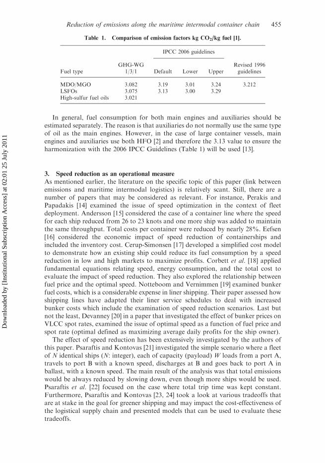
In general, fuel consumption for both main engines and auxiliaries should beestimated separately. The reason is that auxiliaries do not normally use the same typeof oil as the main engines. However, in the case of large container vessels, mainengines and auxiliaries use both HFO [2] and therefore the 3.13 value to ensure theharmonization with the 2006 IPCC Guidelines (Table 1) will be used [13].

3. Speed reduction as an operational measure

As mentioned earlier, the literature on the specific topic of this paper (link betweenemissions and maritime intermodal logistics) is relatively scant. Still, there are anumber of papers that may be considered as relevant. For instance, Perakis andPapadakis [14] examined the issue of speed optimization in the context of fleetdeployment. Andersson [15] considered the case of a container line where the speedfor each ship reduced from 26 to 23 knots and one more ship was added to maintainthe same throughput. Total costs per container were reduced by nearly 28%. Eefsen[16] considered the economic impact of speed reduction of containerships andincluded the inventory cost. Cerup-Simonsen [17] developed a simplified cost modelto demonstrate how an existing ship could reduce its fuel consumption by a speedreduction in low and high markets to maximize profits. Corbett et al. [18] appliedfundamental equations relating speed, energy consumption, and the total cost toevaluate the impact of speed reduction. They also explored the relationship betweenfuel price and the optimal speed. Notteboom and Vernimmen [19] examined bunkerfuel costs, which is a considerable expense in liner shipping. Their paper assessed howshipping lines have adapted their liner service schedules to deal with increasedbunker costs which include the examination of speed reduction scenarios. Last butnot the least, Devanney [20] in a paper that investigated the effect of bunker prices onVLCC spot rates, examined the issue of optimal speed as a function of fuel price andspot rate (optimal defined as maximizing average daily profits for the ship owner).

The effect of speed reduction has been extensively investigated by the authors ofthis paper. Psaraftis and Kontovas [21] investigated the simple scenario where a fleetof N identical ships (N: integer), each of capacity (payload) W loads from a port A,travels to port B with a known speed, discharges at B and goes back to port A inballast, with a known speed. The main result of the analysis was that total emissionswould be always reduced by slowing down, even though more ships would be used.Psaraftis et al. [22] focused on the case where total trip time was kept constant.Furthermore, Psaraftis and Kontovas [23, 24] took a look at various tradeoffs thatare at stake in the goal for greener shipping and may impact the cost-effectiveness ofthe logistical supply chain and presented models that can be used to evaluate thesetradeoffs.

Table 1. Comparison of emission factors kg CO2/kg fuel [1].

Fuel typeGHG-WG

1/3/1

IPCC 2006 guidelines

Default Lower UpperRevised 1996guidelines

MDO/MGO 3.082 3.19 3.01 3.24 3.212LSFOs 3.075 3.13 3.00 3.29High-sulfur fuel oils 3.021


Dow

nloa

ded

by [

Inst

itutio

nal S

ubsc

ript

ion

Acc

ess]

at 0

2:01

25

July

201

1

Our generic approach assumes a container vessel that departs from port A andarrives at port B. There is no need to know the number of ports that the vessel stops

in between. The vessel has covered a total distance of L nm from A to B carrying a

payload W with an average (or constant) speed of V0 (in knots). Port B can be thesame with port A—in that case we are talking about a roundtrip. We also assume

that fuel consumptions are known.

3.1. The impact of speed reduction on total trip timeWe will first investigate the impact of speed reduction on total time. The time thatthe vessel spends at sea depends only on speed while time at port depends on many

factors, such as amount of cargo to be handled, loading and unloading speed, etc.

For the time being, we assume that the time in port is known.The times that the vessel spends at sea and in port are expressed as follows:

At sea: Total time at sea T0 ¼L

24 � V0ðdaysÞ

In port: Total time in port t0 (days).

Thus, the total time is the sum of these two.Now suppose that the ship operator wants to investigate the scenario of speed

reduction. This may be for cost-related reasons or for environmental reasons (todecrease CO2 emissions), or for any other reason as described in Section 3.2.

Reducing speed means that the ship will now sail at a new speed V which will be afraction of the original speed (V¼ aV0 where 05a51) and, hence, there will be an

increase of the total time at sea, T ¼ L24V ¼

T0

a .It is obvious that if time in port remains the same (port time difference t� t0

equals 0), there will be a need to add a number of additional vessels (possiblyfractional) in order to maintain the same throughput per year. In theory, even if

more ships are added in a specific route, it has been proven that this is beneficial forthe operator (but only in terms of bunker costs alone) and for the environment

(reduced emissions). Whether or not speed reduction is overall more profitable to the

operator depends on the additional costs of deploying the extra vessels. Speedreduction will also entail increased in-transit inventory costs, to be borne by the

charterer, and these are proportional to the value of the cargo. For an analysis ofrelated scenarios, see Refs [22, 24].

On the other hand, if time in port could be reduced (t5t0), and in fact if ‘‘t’’ is

such that the total time, including time in port, remains the same Tþ t ¼ T0 þ t0ð Þ,

then there will be no need to add extra ships.It should be realized that reducing port time may not be possible, as this would

depend on a variety of factors that may concern either the ship, or the port itself, or

both. But if time in port can be reduced at all, it can be a crucial factor to reducingship total emissions. To our knowledge, this has not been investigated much in the

literature. An attempt to investigate such scenarios was done by Psaraftis et al. [22].It should be noted that even if the total time cannot be kept constant, any reduction

in port time leads to a decrease of fuel consumption and, thus, to CO2 emissions.

The issue of port time in the quest to reduce emissions will be analyzed into detail inSection 4 and ways to achieve this with optimization of land-side operations and

berthing priority service policies in Sections 5 and 6, respectively.


Dow

nloa

ded

by [

Inst

itutio

nal S

ubsc

ript

ion

Acc

ess]

at 0

2:01

25

July

201

1

3.2. Effect on fuel consumptionIn the above scenario, the daily fuel consumption and the time in port are assumed

known. Furthermore, the time that the ship spends at sea can be calculated given

that distance and speed are known. Thus, the following are known:

At sea:Fuel consumption F0 (tons per day)

Total time at sea T0 ¼L

24 � V0ðdaysÞ

In port:Fuel consumption f (tons per day)Total time in port t0 (days).

The total fuel consumption for this trip is FC0 ¼ F0 � T0 þ f � t0:

As discussed above, after speed reduction, the new speed V will be a fraction of

the original speed (V¼ aV0, where 05a51) and hence there will be an increase of the

time at sea,

T ¼L

24V¼

T0

a:

Realistic values for the speed reduction factor ‘‘a’’ can be in the range 0.8–0.95,

which imply a speed reduction in the range of 5–20%. In general, for such small

speed reductions, the effect of speed change on fuel consumption is assumed cubic

for the same ship. However, many vessels are reported to sail as low as half of the

normal speed. In very low-load cases and in the case of container vessels (having a

design speed of more than 20 knots), a more case-specific speed-to-power

relationship has to be derived (Section 2.2).Generally speaking, the fuel consumption at the reduced speed F can be

approximated as follows:

F

F0¼

V

V0

� �n

given that F0 ¼ kVn0, where k and n are known constants:

Reductions in fuel consumption, emissions, and bunker cost will be presented as a

function of n. Note that as discussed in Section 2.2, for the case of container vessels,

a value of n greater than 3 has to be used.We can compute the difference in fuel consumption for the above scenario as

follows:

At sea:

Dðconsumption at seaÞ ¼ F �T�F0 �T0 ¼ F �L

24 �V�F0 �

L

24 �V0

¼V¼aV0 L

24 �V0F �

1

a�F0

� �¼

FF0¼ V

V0

� �n

L

24 �V0

V

V0

� �n

F0 �1

a�F0

� �

¼L

24 �V0anF0 �

1

a�F0

� �


Dow

nloa

ded

by [

Inst

itutio

nal S

ubsc

ript

ion

Acc

ess]

at 0

2:01

25

July

201

1

In port:

Dðconsumption at portÞ ¼ f � t� f � t0 ¼ f � t� t0ð Þ:

Thus, the total fuel consumption decrease due to slow steaming is

DðFuel consumptionÞ ¼L

24 � V0F0 an�1 � 1� �

þ f � t� t0ð Þ: ð1Þ

Note that the first addend is negative since, by definition, parameter ‘‘a’’ liesbetween 0 and 1 and L, F0 and V0 are always positive.

In the case where time in port is constant, t� t0 is equal to 0 and it decreases(t5t0). This leads to a negative t� t0. Thus, according to (1), for both cases’ speedreduction leads to a decrease in fuel consumption per trip.

3.3. Effect on CO2 emissionsTo find the equivalent CO2 emissions reduction, the reduction in bunker consump-tion has to be multiplied with the appropriate emissions factor (FCO2

) since emissionsare directly related to fuel consumption. As discussed in Section 2.3, in this paper weuse a factor of 3.13, see Ref. [13].

Thus, using Equation (1), the reduction in CO2 emissions is:

DðCO2 emissionsÞ ¼ FCO2�

L

24 � V0F0 an�1 � 1� �

þ f � t� t0ð Þ

� ð2Þ

Note that since the change in fuel consumption is always negative (Section 3.2),there is always a reduction in fuel emissions and in the case where time in port can bedecreased, the reduction is greater than in the case where time in port is keptconstant.

In addition, note that, in general, emissions at sea are much more than emissionsin port. The exact numbers depend on the ship type and size. While in port, shipsconsume much fewer fuel than while sailing and the time that the vessels spend at seais only a small portion of the total trip time for large trips.

3.4. Effect on fuel costsThe fuel cost reduction can be estimated by assuming that the price of the fuel usedby the ship is known and equal to p (assumed constant during the year). Even thoughit is assumed a constant in our analysis, p is very much market-related, and, as such,may fluctuate widely in time, as historical experience has shown. For example,following the economic crisis of mid-2008, in June 2008, the average prices in thePort of Rotterdam for Low-Sulfur Fuel Oil (LSFO; LS 380) and MDO were 644.5and 1126.0 USD/ton, respectively. Prices then collapsed and came to as low as 193.5USD/ton (LSFO) and 420.0 (MDO) in December 2008. Since then, prices have beenincreasing. In January 2010, the average prices are 463.50 and 586USD/ton forLSFO and MDO, respectively.

In any case, the assumption of a constant price causes no loss of generality, as anaverage price can be used. Also, as the ship will generally consume different kinds offuels during the trip and in port assuming a unique fuel price is obviously asimplification. But this causes no loss of generality either, as an average price can beassumed for the general case.


Dow

nloa

ded

by [

Inst

itutio

nal S

ubsc

ript

ion

Acc

ess]

at 0

2:01

25

July

201

1

Using Equation (1), the reduction in fuel is:

Dðfuel costsÞ ¼ p �L

24 � V0F0 an�1 � 1� �

þ f � t� t0ð Þ

� : ð3Þ

4. Container ports: time considerations

As discussed above, the issue of port time in the quest of emissions reduction is veryimportant. First of all, fuel consumption is proportional to the amount of time that avessel spends at sea and in port. Thus, any reduction in the time that a vessel spendsin port yields a reduction in fuel consumption, emissions, and bunker costs. This istrue even in the absence of other operational measures such as speed reduction.In addition, as we discussed before, measures to reduce time in port are, also, verydesirable when implementing speed reduction measures and in extreme cases, thismay help to keep constant total trip times.

It should be realized that reducing port time may not be possible, as this woulddepend on a variety of factors that may concern either the ship, or the port itself, orboth. For example, in the case of ferries [22], especially those engaged in short seashipping, reducing port time comes at no extra cost, as the time that ship stays idle inport can be easily reduced. We can easily implement this under the assumption thatthe speed reduction will only lead to a small increase in total time so that passengerswill still prefer using a ferry instead of other transportation modes, which is a logicalassumption. Furthermore, this is feasible since ferries engaged in domestic sails andshort sea shipping tend to spend a lot of time idle waiting for the next scheduled trip.Plus, reduced speed can lead to reduced fuel costs whose savings can be passed on tothe passenger in terms of reduced ticket prices.

On the other hand, container ports are more advance in structures and proceduresthan other ports and most operations are done in very efficient ways; thus, there isonly a little room for improvement. But if time in port can be reduced at all, it can bea crucial factor to reduce ship total emissions. Note that reduction of port time isalso desirable by port operators since it brings more money to the port by being ableto serve more vessels. Thus, there is an extra incentive for reducing time in port.

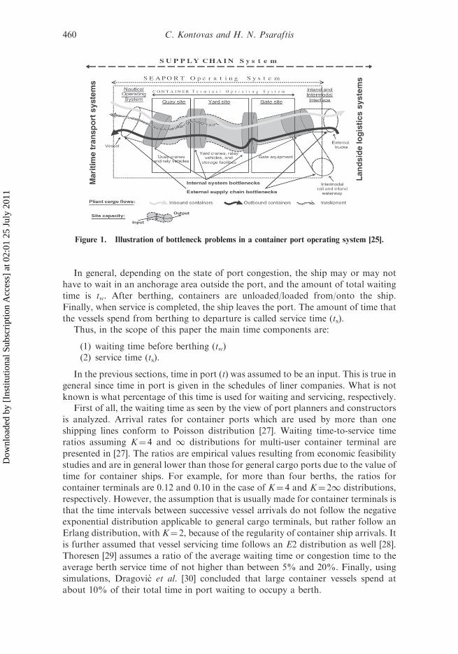
4.1. The container terminal and port time componentsBichou [25] presents the major bottlenecks in a container port (Figure 1). Some ofthese are outside the scope of our study. For instance, once the ship has completedthe loading/unloading procedures she is ready to depart. Transporting the unloadedcontainers to the yard and transhipping them to land-based vehicles are outside thescope of this paper since the time consumed in the above procedures is not includedin the vessel’s turnaround time.

A list of procedures, mainly based on [26] are used in order to identify areas andoperations that are time consuming. There are four possible states for a vessel:arriving, berthing, loading and unloading and, finally, departing. When a vessel thatcarries cargo is approaching the port, she may berth immediately or wait for one ofthe reasons illustrated in the following figure, the most important of which is that theberth may not be available. After berthing, there are also several reasons that canprevent the immediate start of loading or unloading operations. One of them isrelated to the cargo-handling equipment, which may be allocated elsewhere.


Dow

nloa

ded

by [

Inst

itutio

nal S

ubsc

ript

ion

Acc

ess]

at 0

2:01

25

July

201

1

In general, depending on the state of port congestion, the ship may or may not

have to wait in an anchorage area outside the port, and the amount of total waiting

time is tw. After berthing, containers are unloaded/loaded from/onto the ship.

Finally, when service is completed, the ship leaves the port. The amount of time that

the vessels spend from berthing to departure is called service time (ts).Thus, in the scope of this paper the main time components are:

(1) waiting time before berthing (tw)(2) service time (ts).

In the previous sections, time in port (t) was assumed to be an input. This is true in

general since time in port is given in the schedules of liner companies. What is not

known is what percentage of this time is used for waiting and servicing, respectively.First of all, the waiting time as seen by the view of port planners and constructors

is analyzed. Arrival rates for container ports which are used by more than one

shipping lines conform to Poisson distribution [27]. Waiting time-to-service time

ratios assuming K¼ 4 and 1 distributions for multi-user container terminal are

presented in [27]. The ratios are empirical values resulting from economic feasibility

studies and are in general lower than those for general cargo ports due to the value of

time for container ships. For example, for more than four berths, the ratios for

container terminals are 0.12 and 0.10 in the case of K¼ 4 and K¼ 21 distributions,

respectively. However, the assumption that is usually made for container terminals is

that the time intervals between successive vessel arrivals do not follow the negative

exponential distribution applicable to general cargo terminals, but rather follow an

Erlang distribution, with K¼ 2, because of the regularity of container ship arrivals. It

is further assumed that vessel servicing time follows an E2 distribution as well [28].

Thoresen [29] assumes a ratio of the average waiting time or congestion time to the

average berth service time of not higher than between 5% and 20%. Finally, using

simulations, Dragovic et al. [30] concluded that large container vessels spend at

about 10% of their total time in port waiting to occupy a berth.

Figure 1. Illustration of bottleneck problems in a container port operating system [25].


Dow

nloa

ded

by [

Inst

itutio

nal S

ubsc

ript

ion

Acc

ess]

at 0

2:01

25

July

201

1

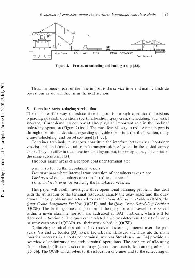
Thus, the biggest part of the time in port is the service time and mainly landsideoperations as we will discuss in the next section.

5. Container ports: reducing service time

The most feasible way to reduce time in port is through operational decisionsregarding quayside operations (berth allocation, quay cranes scheduling, and vesselstowage). Cargo-handling equipment also plays an important role in the loading/unloading operation (Figure 2) itself. The most feasible way to reduce time in port isthrough operational decisions regarding quayside operations (berth allocation, quaycranes scheduling, and vessel stowage) [31, 32].

Container terminals in seaports constitute the interface between sea (containervessels) and land (trucks and trains) transportation of goods in the global supplychain. They do differ in size, function, and layout but, in principle, they all consist ofthe same sub-systems [34].

The four major areas of a seaport container terminal are:

Quay area for berthing container vesselsTransport area where internal transportation of containers takes placeYard area where containers are transferred to and storedTruck and train area for servicing the land-based vehicles.

This paper will briefly investigate three operational planning problems that dealwith the utilization of the terminal resources, namely the quay space and the quaycranes. These problems are referred to as the Berth Allocation Problem (BAP), theQuay Crane Assignment Problem (QCAP), and the Quay Crane Scheduling Problem(QCSP). The berthing time and position at the quay for each vessel to be servedwithin a given planning horizon are addressed in BAP problems, which will bediscussed in Section 6. The quay crane related problems determine the set of cranesto serve each vessel (QCAP) and their work schedule (QCSP).

Optimizing terminal operations has received increasing interest over the pastyears. Vis and de Koster [33] review the relevant literature and illustrate the mainlogistics processes in a container terminal, whereas Steenken et al. [34] provide anoverview of optimization methods terminal operations. The problem of allocatingships to berths (discrete case) or to quays (continuous case) is dealt among others in[35, 36]. The QCSP which refers to the allocation of cranes and to the scheduling of

Figure 2. Process of unloading and loading a ship [33].


Dow

nloa

ded

by [

Inst

itutio

nal S

ubsc

ript

ion

Acc

ess]

at 0

2:01

25

July

201

1

stevedoring operations can be solved with the use of dynamic programming asproposed in [37], or be addressed with a greedy randomized adaptive searchprocedure like the one analyzed in [38]. A branch and cut procedure for this class ofproblems is reported in [39] and the so-called ‘‘double cycling’’ procedures forloading and unloading are described [40]. Furthermore, yard operations such asstorage policies and the design of re-marshalling are also of great importance. Leeet al. [41] address a yard storage allocation problem to reduce traffic congestion and[42] presents a model for container re-marshalling. For a review of the operationresearch literature of problems related to container terminal management, the readermay refer among others to Vis and de Koster [33] and Steenken et al. [34]. Anotherliterature survey of this broad class of problems, with some 157 related references, ispresented in Stahlblock and Voss [43]. Recently, Bierwirth and Meisel [44] present asurvey of berth allocation and QCSPs in container terminals with particular focuson integrated solution approaches. Finally, following the trend of automation ofseaport container terminals, several studies have investigated automation oncontainer-handling systems. For more information, the reader is referred toGunther and Kim [45].

6. Container ports: reducing waiting time under an alternative service policy

This section deals with service policies that affect the waiting time before berthing.Port managers in container terminals attempt to reduce costs by efficiently utilizingport resources. Among all the resources, berths are the most important resources andgood berth scheduling improves customers’ satisfaction and increases port through-put, thus, leads to higher revenues. The usage of berths is scheduled by an intuitivetrial-and-error method and varies from terminal to terminal.

Also, terminal operators usually have different priorities for different types ofvessels. The priorities can be considered in BAP by converting them into costcoefficients of the penalty cost for vessels in the objective function. The mostcommonly used berthing priority policies are:

(1) FCFS(2) Minimizing total completion time(3) Maximization of total profit—Giving priority to bigger vessels(4) Berthing closest to stack(5) Priority service to big customers.

The traditional BAPs focus on the FCFS policy. In practice, this is the mostcommonly used policy for ports worldwide except for the case where ports have fixedassignments/berths to shipping lines. Another priority of the port manager may be tominimize total completion time. Allocating vessels to berths by simply minimizingthe total time can lead to problems where vessels with smaller handling volumevessels (e.g., feeders) are receiving higher priorities than vessels with larger handlingvolumes which end up serviced at the end of the queues at each berth. Maximizationof total profits can be achieved by giving priority to bigger vessels (that are moreprofitable than the smaller ones) or to smaller vessels (e.g., feeders) that have lessservice time and thus more ships are serviced in a given time. Other ports try to berthships close to the storage location of the containers to be loaded.

In the recent scientific literature, very little has been written on the interface ofBAP and emissions. Imai et al. [46] tried to modify the existing formulation of the


Dow

nloa

ded

by [

Inst

itutio

nal S

ubsc

ript

ion

Acc

ess]

at 0

2:01

25

July

201

1

BAP in order to treat calling vessels at various service priorities, however, withoutrelating this to minimization of port emissions. Recently, in [47], the discrete spaceand dynamic BSP where vessel arrival time is optimized to account for theminimization of port-related emissions, waiting time of vessels and delayeddepartures were studied. Alvarez et al. [48] present a hybrid simulation–optimizationapproach for evaluating berthing priority and speed optimization policies in amarine terminal and compare three berthing priority policies: FCFS, standardizedestimated arrival time, and global Optimization of Speed Berth, and EquipmentAllocations (GOSBEA).

Lately, many customers have contracts with the terminal operators that ensurethem guaranteed Berth-On-Arrival (BOA) service— that is, the actual berthingoccurs within two hours of arrival. In this case, the objective of berth scheduling is tominimize the penalty cost resulting from delays in the departures of those vessels andthe additional handling costs resulting from non-optimal locations of vessels.Carriers usually inform the terminal operator on the Expected Arrival Time (ETA)and the requested departure time of vessels. Based on the information, the terminaloperator tries to meet the requested departure time of all other vessels. However,when the arrival rate of vessels is high or when unexpected arrivals occur, it is notpossible to complete services as pre-scheduled.

A related strategy is a policy in which a line could book a berthing time slot inadvance and guaranteed service in that slot. In a seminal paper, Psaraftis [49]describes his experience from the real world when he was put in charge of the PiraeusPort Authority (PPA). The PPA was thinking of switching from the common policyof FCFS (first come, first served) to a system in which a line could book a berthingtime slot in advance and to be guaranteed service in that slot. The originalmotivation was that this system would streamline utilization of cranes during peakperiods and would effectively increase the capacity of the terminal. This scheme isreferred to as ‘‘Booking by rendezvous’’.

The rationale for such a scheme can be understood by the fact that demand for aterminal’s resources is by no means constant, as it is subject to the randomness ofship arrivals. To have adequate reserve capacity so as to meet peaks in demandwithout congestion, the terminal would have to invest into additional cargo-handlingequipment, more piers, etc, which is a decision of strategic nature involving highinvestment costs. Before such a decision is contemplated, a natural considerationwould be to see if the peaks in demand can be streamlined by an appropriatereallocation of traffic. Such a streamlining would reduce congestion and also reduceport costs due to overtime pay, among other things.

Streamlining the peaks in demand is the main objective of the ‘‘booking byrendezvous’’ system. The scheme is a way to minimize disruption, smoothen portdemand peaks and maximize efficiency with the prompt berthing of vessels uponarrival. According to the scheme, a ship books service in advance, by declaring thatthe ship would arrive at the terminal at a prespecified date and time. If the ship ispunctual in the rendezvous, the terminal guarantees berthing on arrival, bypassingother ships that have not booked, with a pre-arranged number of gantry cranes. Ifthe ship misses the rendezvous, it is back in the queue together with all other ships.

In Piraeus, the system was implemented for the container terminal and the carterminal for the first time in 1999, and involved the allocation of one-third of bothterminals to the scheme, and an advance notice of no less than 5 days before arrival(and in special cases 3 days). It is clear that the scheme was geared more to large


Dow

nloa

ded

by [

Inst

itutio

nal S

ubsc

ript

ion

Acc

ess]

at 0

2:01

25

July

201

1

mainline ships coming from distant destinations rather than smaller feeder ships, asthe latter are unable to predict with accuracy their schedule 5 days in advance, as thisdepends on the situation in previous ports. There was high demand for the scheme byshipping companies, with request to extend it by lowering the required notice of5 days, something that was not possible at the time. With the acquisition of 4 moregantry cranes, in 2002, the system was abolished, only to be introduced again inlater years but not on a permanent basis. Other ports also have this scheme orvariants of it.

Thus, given the ‘‘booking by rendezvous’’ the time in port is reduced by tw.Therefore, the reduction in port time is: Dt ¼ t� t0 ¼ �tw and the relative reductionin fuel consumption, costs, and emissions can be calculated as follows (Section 3).

In port (reductions by using the ‘‘Booking by rendezvous’’)

DðFuel consumptionÞ ¼ �f � tw ð4Þ

Dðfuel costsÞ ¼ �p � f � tw ð5Þ

DðCO2 emissionsÞ ¼ �FCO2� f � tw: ð6Þ

We shall now attempt to analyze the effect of this system as a way to help theimplementation of speed reduction measures. Clearly, it would not make sense for acontainer vessel to speed to a port only to have to wait there because of congestion. Ifthe ship can book by rendezvous, savings in fuel (and emissions) can be realized andcongestion can be avoided at the same time.

Let us assume that a vessel is engaged in the container market. Assume also asbefore that after the implementation of speed reduction (time at sea increases), thetime in port is reduced by tw. Given that the reduction in port time is t� t0 ¼ �tw,Equations (1)–(3) can be used to estimate the reduction in fuel consumption, fuelcosts, and emissions as follows:

DðFuel consumptionÞ ¼L

24 � V0F0 an�1 � 1� �

� f � tw ð7Þ

Dðfuel costsÞ ¼ p �L

24 � V0F0 an�1 � 1� �

� f � tw

� ð8Þ

DðCO2 emissionsÞ ¼ FCO2�

L

24 � V0F0 an�1 � 1� �

� f � tw

� : ð9Þ

As one may notice, the first addend is negative since, by definition, parameter ‘‘a’’lies between 0 and 1 and L, F0, and V0 are always positive thus there will always be areduction in fuel consumption, bunker cost, and emissions. Finally, note that theliner company is benefited by this scheme since there is a reduction in fuel costs andthe port increases port throughput, thus, leading to higher revenues. In this ‘‘win–win’’ scenario, the environment and society are also benefited from the reduction inCO2 emissions.

6.1. An exampleOur example is based on a real route, the North Europe–Asia route AE1 routeserved by the CKYH alliance (Figure 3). The AE1 route covers nine ports on the


Dow

nloa

ded

by [

Inst

itutio

nal S

ubsc

ript

ion

Acc

ess]

at 0

2:01

25

July

201

1

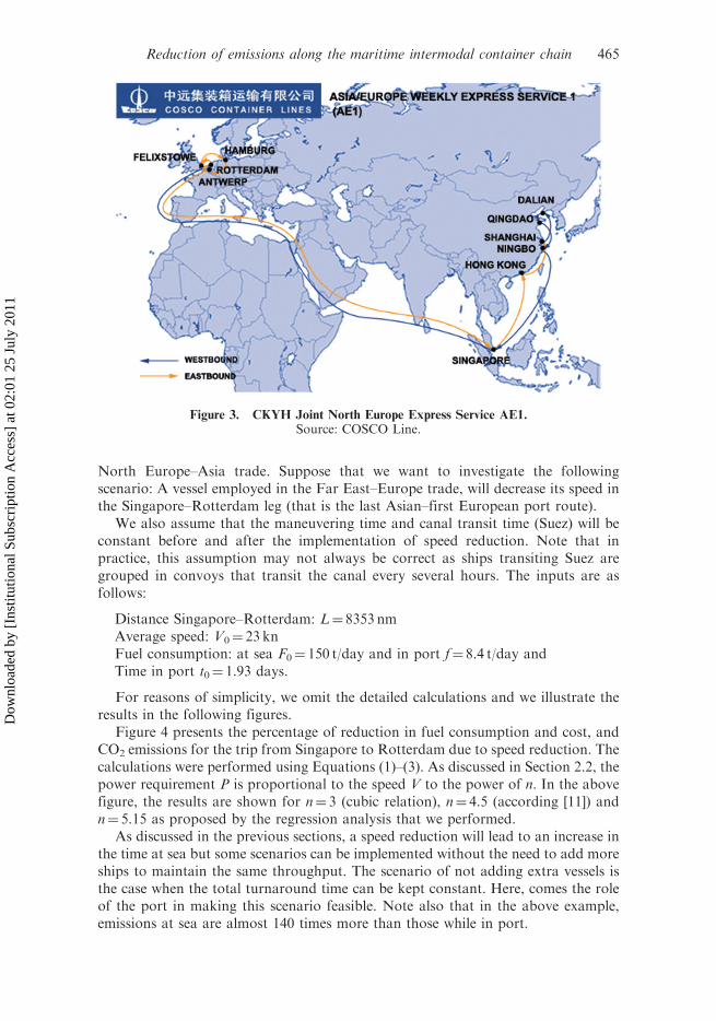
North Europe–Asia trade. Suppose that we want to investigate the followingscenario: A vessel employed in the Far East–Europe trade, will decrease its speed inthe Singapore–Rotterdam leg (that is the last Asian–first European port route).

We also assume that the maneuvering time and canal transit time (Suez) will beconstant before and after the implementation of speed reduction. Note that inpractice, this assumption may not always be correct as ships transiting Suez aregrouped in convoys that transit the canal every several hours. The inputs are asfollows:

Distance Singapore–Rotterdam: L¼ 8353 nmAverage speed: V0¼ 23 knFuel consumption: at sea F0¼ 150 t/day and in port f¼ 8.4 t/day andTime in port t0¼ 1.93 days.

For reasons of simplicity, we omit the detailed calculations and we illustrate theresults in the following figures.

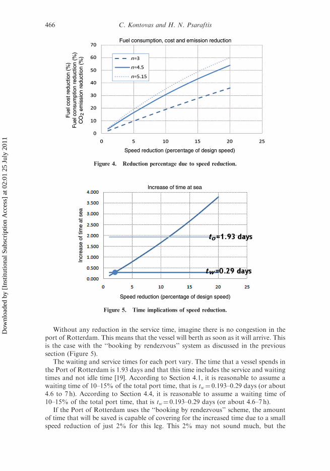
Figure 4 presents the percentage of reduction in fuel consumption and cost, andCO2 emissions for the trip from Singapore to Rotterdam due to speed reduction. Thecalculations were performed using Equations (1)–(3). As discussed in Section 2.2, thepower requirement P is proportional to the speed V to the power of n. In the abovefigure, the results are shown for n¼ 3 (cubic relation), n¼ 4.5 (according [11]) andn¼ 5.15 as proposed by the regression analysis that we performed.

As discussed in the previous sections, a speed reduction will lead to an increase inthe time at sea but some scenarios can be implemented without the need to add moreships to maintain the same throughput. The scenario of not adding extra vessels isthe case when the total turnaround time can be kept constant. Here, comes the roleof the port in making this scenario feasible. Note also that in the above example,emissions at sea are almost 140 times more than those while in port.

Figure 3. CKYH Joint North Europe Express Service AE1.Source: COSCO Line.


Dow

nloa

ded

by [

Inst

itutio

nal S

ubsc

ript

ion

Acc

ess]

at 0

2:01

25

July

201

1

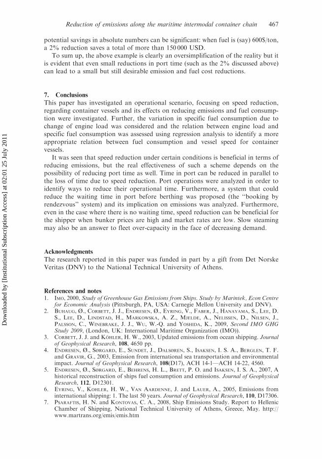
Without any reduction in the service time, imagine there is no congestion in theport of Rotterdam. This means that the vessel will berth as soon as it will arrive. Thisis the case with the ‘‘booking by rendezvous’’ system as discussed in the previoussection (Figure 5).

The waiting and service times for each port vary. The time that a vessel spends inthe Port of Rotterdam is 1.93 days and that this time includes the service and waitingtimes and not idle time [19]. According to Section 4.1, it is reasonable to assume awaiting time of 10–15% of the total port time, that is tw¼ 0.193–0.29 days (or about4.6 to 7 h). According to Section 4.4, it is reasonable to assume a waiting time of10–15% of the total port time, that is tw¼ 0.193–0.29 days (or about 4.6–7 h).

If the Port of Rotterdam uses the ‘‘booking by rendezvous’’ scheme, the amountof time that will be saved is capable of covering for the increased time due to a smallspeed reduction of just 2% for this leg. This 2% may not sound much, but the

Figure 5. Time implications of speed reduction.

Figure 4. Reduction percentage due to speed reduction.


Dow

nloa

ded

by [

Inst

itutio

nal S

ubsc

ript

ion

Acc

ess]

at 0

2:01

25

July

201

1

potential savings in absolute numbers can be significant: when fuel is (say) 600$/ton,a 2% reduction saves a total of more than 150 000 USD.

To sum up, the above example is clearly an oversimplification of the reality but itis evident that even small reductions in port time (such as the 2% discussed above)can lead to a small but still desirable emission and fuel cost reductions.

7. Conclusions

This paper has investigated an operational scenario, focusing on speed reduction,regarding container vessels and its effects on reducing emissions and fuel consump-tion were investigated. Further, the variation in specific fuel consumption due tochange of engine load was considered and the relation between engine load andspecific fuel consumption was assessed using regression analysis to identify a moreappropriate relation between fuel consumption and vessel speed for containervessels.

It was seen that speed reduction under certain conditions is beneficial in terms ofreducing emissions, but the real effectiveness of such a scheme depends on thepossibility of reducing port time as well. Time in port can be reduced in parallel tothe loss of time due to speed reduction. Port operations were analyzed in order toidentify ways to reduce their operational time. Furthermore, a system that couldreduce the waiting time in port before berthing was proposed (the ‘‘booking byrendezvous’’ system) and its implication on emissions was analyzed. Furthermore,even in the case where there is no waiting time, speed reduction can be beneficial forthe shipper when bunker prices are high and market rates are low. Slow steamingmay also be an answer to fleet over-capacity in the face of decreasing demand.

Acknowledgments

The research reported in this paper was funded in part by a gift from Det NorskeVeritas (DNV) to the National Technical University of Athens.

References and notes1. IMO, 2000, Study of Greenhouse Gas Emissions from Ships. Study by Marintek, Econ Centre

for Economic Analysis (Pittsburgh, PA, USA: Carnegie Mellon University and DNV).2. BUHAUG, Ø., CORBETT, J. J., ENDRESEN, Ø., EYRING, V., FABER, J., HANAYAMA, S., LEE, D.

S., LEE, D., LINDSTAD, H., MARKOWSKA, A. Z., MJELDE, A., NELISSEN, D., NILSEN, J.,PALSSON, C., WINEBRAKE, J. J., WU, W.-Q. and YOSHIDA, K., 2009, Second IMO GHGStudy 2009, (London, UK: International Maritime Organization (IMO)).

3. CORBETT, J. J. and KOHLER, H. W., 2003, Updated emissions from ocean shipping. Journalof Geophysical Research, 108, 4650 pp.

4. ENDRESEN, Ø., SØRGARD, E., SUNDET, J., DALSØREN, S., ISAKSEN, I. S. A., BERGLEN, T. F.and GRAVIR, G., 2003, Emission from international sea transportation and environmentalimpact. Journal of Geophysical Research, 108(D17), ACH 14-1––ACH 14-22, 4560.

5. ENDRESEN, Ø., SØRGARD, E., BEHRENS, H. L., BRETT, P. O. and ISAKSEN, I. S. A., 2007, Ahistorical reconstruction of ships fuel consumption and emissions. Journal of GeophysicalResearch, 112, D12301.

6. EYRING, V., KOHLER, H. W., VAN AARDENNE, J. and LAUER, A., 2005, Emissions frominternational shipping: 1. The last 50 years. Journal of Geophysical Research, 110, D17306.

7. PSARAFTIS, H. N. and KONTOVAS, C. A., 2008, Ship Emissions Study. Report to HellenicChamber of Shipping, National Technical University of Athens, Greece, May. http://www.martrans.org/emis/emis.htm


Dow

nloa

ded

by [

Inst

itutio

nal S

ubsc

ript

ion

Acc

ess]

at 0

2:01

25

July

201

1

8. PSARAFTIS, H. N. and KONTOVAS, C. A., 2009, CO2 emissions statistics for the worldcommercial fleet. WMU Journal of Maritime Affairs, 8(1), 1–25.

9. MAN DIESEL, 2008, Low Container Ship Speed Facilitated by Versatile ME/ME-CEngines. MAN Diesel A/S Report, Copenhagen, Denmark, January.

10. BARRASS, C. B., 2004, Ship Design and Performance for Masters and Mates (Oxford:Elsevier).

11. MAN DIESEL, 2006, Ship Propulsion – Basic Principles of Ship Propulsion. MAN DieselA/S Report, Copenhagen, Denmark, August.

12. NOTTEBOOM, T. and CARIOU, P., 2009, Fuel surcharge practices of container shippinglines: Is it about cost recovery or revenue-making? In Proceedings of the IAME2009Conference, International Association of Maritime Economists, June 2009, Copenhagen.

13. IMO, 2008, Liaison with the Secretariats of UNFCCC and IPCC concerning the Carbonto CO2 conversion Factor. MEPC 58/4/3.

14. PERAKIS, A. N. and PAPADAKIS, N., 1987, Fleet deployment optimization models, part 1.Maritime Policy and Management, 14(2), 127–144.

15. ANDERSSON, L., 2008, Economies of Scale with Ultra Large Container Vessels. MBAassignment no 3, The Blue MBA, Copenhagen Business School.

16. EEFSEN, T., 2008, Container Shipping: Speed, Carbon Emissions and Supply Chain.MBA assignment no 2, The Blue MBA, Copenhagen Business School.

17. CERUP-SIMONSEN, B., 2008, Effects of Energy Cost and Environmental Demands onFuture Shipping Markets. MBA assignment no 3, The Blue MBA, Copenhagen BusinessSchool.

18. CORBETT, J., WANG, H. and WINEBRAKE, J., 2009, Impacts of speed reductions on vessel-based emissions for international shipping. In Proceedings of Transportation ResearchBoard Annual Meeting, Washington, DC.

19. NOTTEBOOM, T. E. and VERNIMMEN, B., 2009, The effect of high fuel costs on liner serviceconfiguration in container shipping. Journal of Transport Geography, 17, 325–337.

20. DEVANNEY, J. W., 2010, The impact of bunker prices on VLCC spot rates. In Proceedingsof the 3rd International Symposium on Ship Operations, Management and Economics,SNAME Greek Section, October 7–8, Athens, Greece.

21. PSARAFTIS, H. N. and KONTOVAS, C. A., 2009, Ship emissions: Logistics and othertradeoffs. In Proceedings of the 10th International Marine Design Conference (IMDC2009), Trondheim, Norway, May.

22. PSARAFTIS, H. N., KONTOVAS, C. A. and KAKALIS, N., 2009, Speed reduction as anemissions reduction measure for fast ships. In Proceedings of the 10th InternationalConference on Fast Transportation (FAST 2009), October 5–8, Athens, Greece.

23. PSARAFTIS, H. N. and KONTOVAS, C. A., 2009, Green maritime logistics: Cost-effectiveness of speed reductions and other emissions reduction measures. InProceedings of the International Symposium on Maritime Logistics and Supply ChainSystems 2009, April 23–24, Singapore.

24. PSARAFTIS, H. N. and KONTOVAS, C. A., 2010, Balancing the economic and environmentalperformance of maritime transportation. Transportation Research Part D, 15(8),458–462.

25. BICHOU, K., 2006, Review of performance approaches and a supply chain framework toport performance benchmarking. In Port Governance and Port Performance, edited byM. Brooks and K. Cullinane, Research in Transportation Economics, Vol. 17 (London:Elsevier), pp. 567–99.

26. AGERSCHOU, H. (ed.), 1983, Planning and Design of Ports and Marine Terminals (London,UK: John Wiley).

27. AGERSCHOU, H. (ed.), 2004, Planning and Design of Ports and Marine Terminals (London,UK: Thomas Telford Ltd).

28. TSINKER, G. P., 2004, Port Engineering: Planning, Construction, Maintenance, andSecurity (Hoboken, NJ: Wiley).

29. THORESEN, C., 2003, Port Designer’s Handbook (London, UK: Thomas Telford Ltd).30. DRAGOVIC, B., PARK, N. K., RADMILOVIC, Z. R. and MARAS, V., 2005, Simulation

modeling of ship-berth link with priority service. Maritime Economics and Logistics, 7(4),316–335.


Dow

nloa

ded

by [

Inst

itutio

nal S

ubsc

ript

ion

Acc

ess]

at 0

2:01

25

July

201

1

31. NOTTEBOOM, T. E., 2006, The time factor in liner shipping services. Maritime Economicsand Logistics, 8, 19–39.

32. LAINE, J. T. and VEPSALAINEN, A. P. J., 1994, Economies of speed in sea transportation.International Journal of Phcal Distribution and Logistic Management, 24(8), 33–41.

33. VIS, I. and DE KOSTER, R., 2003, Transshipment of containers at a container terminal: Anoverview. European Journal of Operational Research, 147, 1–16.

34. STEENKEN, D., VOSS, S. and STAHLBOCK, R., 2004, Container terminal operation andoperations research – a classification and literature review. OR Spectrum, 26, 3–49.

35. CORDEAU, J., GAUDIOSO, M., LAPORTE, G. and MOCCIA, L., 2007, The service allocationproblem at the Gioia Tauro maritime terminal. European Journal of OperationalResearch, 176, 1167–1184.

36. WANG, F. and LIM, A., 2007, A stochastic beam search for the berth allocation problem.Decision Support Systems, 42, 2186–2196.

37. LIM, A., RODRIGUES, B., XIAO, F. and ZHU, Y., 2004, Crane scheduling with spatialconstraints. Naval Research Logistics, 51, 386–406.

38. KIM, K. H. and PARK, Y. M., 2004, A crane scheduling method for port containerterminal. European Journal of Operational Research, 156, 752–768.

39. MOCCIA, L., CORDEAU, J.-F., GAUDIOSO, M. and LAPORTE, G., 2006, A branch and cutalgorithm for the quay crane scheduling problem in a container terminal. Naval ResearchLogistics, 53, 45–59.

40. GOODCHILD, A. V. and DAGANZO, C. F., 2006, Double cycling strategies for containerships and their effect on ship loading and unloading operation. Transportation Science,40, 473–483.

41. LEE, L., CHEW, E., TAN, K. and HAN, Y., 2006, An optimization model for storage yardmanagement in transshipment hubs. OR Spectrum, 28, 539–561.

42. LEE, Y. and HSU, N.-Y., 2007, An optimization model for the container pre-marshallingproblem. Computers and Operations Research, 34, 3295–3313.

43. STAHLBLOCK, R. and VOSS, S., 2007, Vehicle routing problems and container terminaloperations – An update of research. In The Vehicle Routing Problem: Latest Advancesand New Challenges, edited by B. Golden, S. Raghavan and E. Wasil (New York:Springer Verlag).

44. BIERWIRTH, C. and MEISEL, F., 2010, A survey of berth allocation and quay cranescheduling problems in container terminals. European Journal of Operational Research,202, 615–627.

45. GUNTHER, H. O. and KIM, K. H., 2005, Container Terminals and Automated TransportSystems (New York: Springer Verlag).

46. IMAI, A., NISHIMURA, E. and PAPADIMITRIOU, S., 2003, Berth allocation with servicepriority. Transportation Research Part B, 37, 437–457.

47. GOLIAS, M., SAHARIDIS, G., BOILE, M., THEOFANIS, S. and IERAPETRITOU, M., 2009, Theberth allocation problem: Optimizing vessel arrival time. Maritime Economics andLogistics, 11, 358–377.

48. ALVAREZ, J. F., LONGVA, T. and ENGEBRETHSEN, S., 2010, A methodology to assess vesselberthing and speed optimization policies. Maritime Economics and Logistics, 12,327–346.

49. PSARAFTIS, H. N., 1998, When a port calls . . . an operations researcher answers. OR/MSToday, 25(2), 38–41.


Dow

nloa

ded

by [

Inst

itutio

nal S

ubsc

ript

ion

Acc

ess]

at 0

2:01

25

July

201

1

Documents

Reduction of emissions along the maritime intermodal ... · PDF fileReduction of emissions along the maritime intermodal container chain: ... number of such documents, ... Reduction