Embed Size (px)
Citation preview
Melissa MolnarOhio University, Athens, Ohio
C. John MarekGlenn Research Center, Cleveland, Ohio
Reduced Equations for Calculatingthe Combustion Rates of Jet-Aand Methane Fuel
NASA/TM—2003-212702
November 2003
https://ntrs.nasa.gov/search.jsp?R=20030112865 2018-05-14T22:36:59+00:00Z

The NASA STI Program Office . . . in Profile
Since its founding, NASA has been dedicated tothe advancement of aeronautics and spacescience. The NASA Scientific and TechnicalInformation (STI) Program Office plays a key partin helping NASA maintain this important role.
The NASA STI Program Office is operated byLangley Research Center, the Lead Center forNASA’s scientific and technical information. TheNASA STI Program Office provides access to theNASA STI Database, the largest collection ofaeronautical and space science STI in the world.The Program Office is also NASA’s institutionalmechanism for disseminating the results of itsresearch and development activities. These resultsare published by NASA in the NASA STI ReportSeries, which includes the following report types:
∑ TECHNICAL PUBLICATION. Reports ofcompleted research or a major significantphase of research that present the results ofNASA programs and include extensive dataor theoretical analysis. Includes compilationsof significant scientific and technical data andinformation deemed to be of continuingreference value. NASA’s counterpart of peer-reviewed formal professional papers buthas less stringent limitations on manuscriptlength and extent of graphic presentations.
∑ TECHNICAL MEMORANDUM. Scientificand technical findings that are preliminary orof specialized interest, e.g., quick releasereports, working papers, and bibliographiesthat contain minimal annotation. Does notcontain extensive analysis.
∑ CONTRACTOR REPORT. Scientific andtechnical findings by NASA-sponsoredcontractors and grantees.
∑ CONFERENCE PUBLICATION. Collectedpapers from scientific and technicalconferences, symposia, seminars, or othermeetings sponsored or cosponsored byNASA.
∑ SPECIAL PUBLICATION. Scientific,technical, or historical information fromNASA programs, projects, and missions,often concerned with subjects havingsubstantial public interest.
∑ TECHNICAL TRANSLATION. English-language translations of foreign scientificand technical material pertinent to NASA’smission.
Specialized services that complement the STIProgram Office’s diverse offerings includecreating custom thesauri, building customizeddatabases, organizing and publishing researchresults . . . even providing videos.
For more information about the NASA STIProgram Office, see the following:
∑ Access the NASA STI Program Home Pageat http://www.sti.nasa.gov
∑ E-mail your question via the Internet [email protected]
∑ Fax your question to the NASA AccessHelp Desk at 301–621–0134
∑ Telephone the NASA Access Help Desk at301–621–0390
∑ Write to: NASA Access Help Desk NASA Center for AeroSpace Information 7121 Standard Drive Hanover, MD 21076
Melissa MolnarOhio University, Athens, Ohio
C. John MarekGlenn Research Center, Cleveland, Ohio
Reduced Equations for Calculatingthe Combustion Rates of Jet-Aand Methane Fuel
NASA/TM—2003-212702
November 2003
National Aeronautics andSpace Administration
Glenn Research Center

Available from
NASA Center for Aerospace Information7121 Standard DriveHanover, MD 21076
National Technical Information Service5285 Port Royal RoadSpringfield, VA 22100
This report contains preliminaryfindings, subject to revision as
analysis proceeds.
Available electronically at http://gltrs.grc.nasa.gov
The Propulsion and Power Program atNASA Glenn Research Center sponsored this work.
NASA/TM�2003-212702 1
Reduced Equations for Calculating the Combustion Rates of Jet-A and Methane Fuel
Melissa Molnar Ohio University
Athens, Ohio 45701
C. John Marek National Aeronautics and Space Administration
Glenn Research Center Cleveland, Ohio 44135
ABSTRACT
Simplified kinetic schemes for Jet-A and methane fuels were developed to be used in numerical combustion codes, such as the National Combustor Code (NCC) that is being developed at Glenn. These kinetic schemes presented here result in a correlation that gives the chemical kinetic time as a function of initial overall cell fuel/air ratio, pressure and temperature. The correlations would then be used with the turbulent mixing times to determine the limiting properties and progress of the reaction.
A similar correlation was also developed using data from the NASA�s Chemical Equilibrium Applications (CEA) code to determine the equilibrium concentration of carbon monoxide as a function of fuel air ratio, pressure and temperature.
The NASA Glenn GLSENS kinetics code calculates the reaction rates and rate constants for each species in a kinetic scheme for finite kinetic rates. These reaction rates and the values obtained from the equilibrium correlations were then used to calculate the necessary chemical kinetic times. Chemical kinetic time equations for fuel, carbon monoxide and NOx were obtained for both Jet-A fuel and methane. Introduction
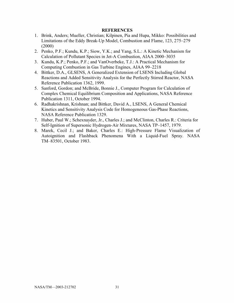
Reaction rates are kinetically limited at low temperatures and mixing limited at very high temperatures. According to the Magnussen model (reference 1), the fuel oxidation rate will be determined by the maximum of either the kinetic time or the turbulent mixing times of the fuel and air. However, for large numerical solutions it is very tedious to use complete classical calculations to compare both the kinetic and turbulent mixing times to determine the region of the reaction. Conventional chemical kinetic schemes are extremely time consuming for two and three dimensional computer calculations for combustors. Large mechanisms with many intermediate species and very fast radical reactions cause the equations to be stiff (extremely fast compared to the overall rate, requiring a large number of small time steps), making them very difficult to integrate. Calculations for these extensive mechanisms are repetitive and complex. Using the simplified kinetic scheme developed here to calculate the three chemical kinetic times greatly reduces the amount of time required to compare kinetic reaction times with turbulent mixing times and will reduce the time required to obtain a converged solution. The advantage of computing the chemical kinetic time for only the species of interest is
NASA/TM�2003-212702 2
that we have only the differential equations of interest to solve, resulting in a much smaller set of equations.
This method is for use in Computational Fluid Dynamics (CFD) calculations where chemical kinetics is important. The current version of NCC requires the user to decide to use either chemical kinetics or the turbulent mixing rates. Following conventional methods would not allow for the calculation of both in a reasonable amount of time. The derived method allows for a quick and easy comparison over the complete spectrum of conditions. This scheme is intended for use in numerical combustion codes, but it can also be used as a quick and accurate method to calculate chemical reaction rates.
We have also curve fitted the equilibrium concentrations of CO, O2, and NOx using data generated by the NASA Chemical Equilibrium Application code (CEA). The CO equilibrium correlation was then used in the calculation of the chemical kinetic time. Although this research focused on Jet-A Fuel and methane, this method may be used for any system. Jet-A fuel was represented as C12H23 , using Krishna Kundu�s twenty three step mechanism (reference 2 and 3). GLSENS (reference 4) was used to integrate the system of equations, at over 400 conditions to derive the rate expressions. It may be reasoned that the presented equations are only as good as the overall mechanism that calculates the data. However, performing the calculations in the conventional manner is also only as good as the mechanism equations and constants that go into them. Simple Time Model The simple model derived here is to be used with the Magnussen mixing model of combustion (reference 1). The turbulent mixing time is shown as a function of the reaction�s turbulent kinetic energy and dissipation rate.
Net rate ),,( kineticf
oxygenfuelr r
yk
Ayk
Amin ϖεεϖ = (1)
Where εA
k equals the turbulent mixing time, τm. The mixing constant, A, is usually
given as 4.0. The factor kineticϖ
fuely is the chemical kinetic time τc.
In order to obtain the chemical source term rϖ , a comparison is made of the mixing rate,
mτ1 and the chemical kinetic rate
cτ1
, and the lowest rate or the longest time is used in
the expression; see Figure 1. This may also be represented by the following relationship: τ = max (τm, τc) (2)
NASA/TM�2003-212702 3
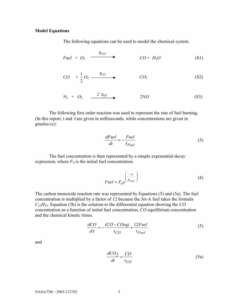
Model Equations The following equations can be used to model the chemical system.
τFuel Fuel + O2 CO + H2O (S1)
CO + 21 O2 CO2 (S2)
N2 + O2 2NO (S3) The following first order reaction was used to represent the rate of fuel burning.
(In this report, t and τ are given in milliseconds, while concentrations are given in gmoles/cc):
(3)
The fuel concentration is then represented by a simple exponential decay
expression, where F0 is the initial fuel concentration. (4) The carbon monoxide reaction rate was represented by Equations (5) and (5a). The fuel concentration is multiplied by a factor of 12 because the Jet-A fuel takes the formula C12H23. Equation (5b) is the solution to the differential equation showing the CO concentration as a function of initial fuel concentration, CO equilibrium concentration and the chemical kinetic times. (5) and
COτ
COdt
2dCO= (5a)
−
= Fuel
t
oeFFuel τ
FuelCO τFuel
τCOeq)(CO
ddCO 12+−−=
τ
Fuel
Fueldt
dFuelτ
−=
τCO
2 τNO
NASA/TM�2003-212702 4
f
COf
COo
COf
COoeqCOeq
τt
eτττ12F)
τττ12FCO0)(CO(tτ
t
eCOCO−
−+
−−−=
−
=− (5b)
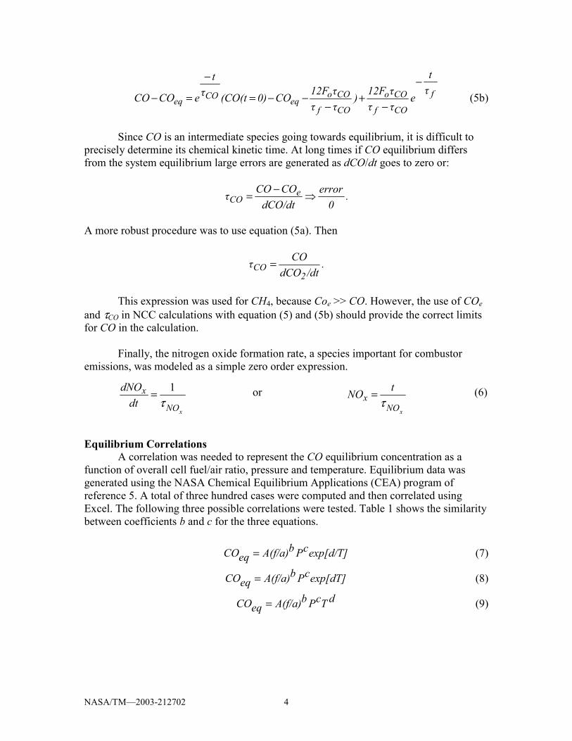
Since CO is an intermediate species going towards equilibrium, it is difficult to precisely determine its chemical kinetic time. At long times if CO equilibrium differs from the system equilibrium large errors are generated as dCO/dt goes to zero or:
.0
errordCO/dt
COCOτ eCO ⇒
−=
A more robust procedure was to use equation (5a). Then
./dtdCO
COτ2
CO =
This expression was used for CH4, because Coe >> CO. However, the use of COe and τCO in NCC calculations with equation (5) and (5b) should provide the correct limits for CO in the calculation. Finally, the nitrogen oxide formation rate, a species important for combustor emissions, was modeled as a simple zero order expression. or (6) Equilibrium Correlations A correlation was needed to represent the CO equilibrium concentration as a function of overall cell fuel/air ratio, pressure and temperature. Equilibrium data was generated using the NASA Chemical Equilibrium Applications (CEA) program of reference 5. A total of three hundred cases were computed and then correlated using Excel. The following three possible correlations were tested. Table 1 shows the similarity between coefficients b and c for the three equations.
exp[d/T]cPbA(f/a)eqCO = (7)
exp[dT]cPbA(f/a)eqCO = (8)
dTcPbA(f/a)eqCO = (9)
xNO
xdt
dNOτ
1=xNO
xtNO
τ=
NASA/TM�2003-212702 5
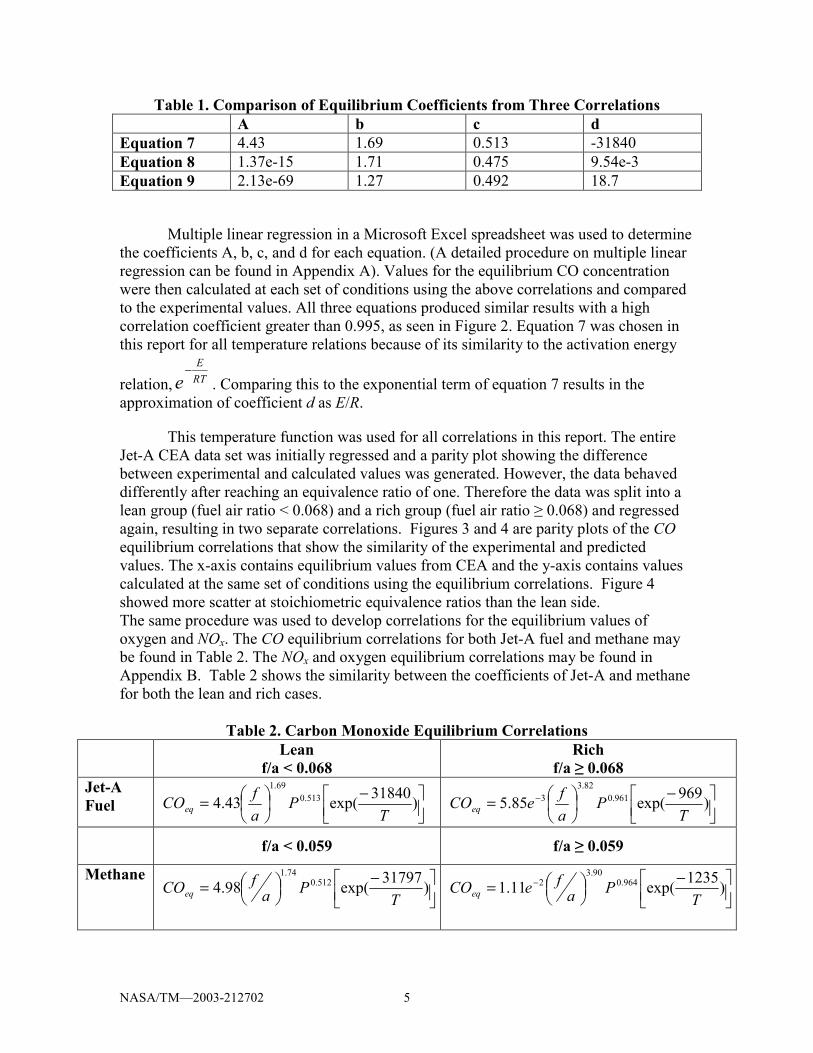
Table 1. Comparison of Equilibrium Coefficients from Three Correlations A b c d Equation 7 4.43 1.69 0.513 -31840 Equation 8 1.37e-15 1.71 0.475 9.54e-3 Equation 9 2.13e-69 1.27 0.492 18.7
Multiple linear regression in a Microsoft Excel spreadsheet was used to determine the coefficients A, b, c, and d for each equation. (A detailed procedure on multiple linear regression can be found in Appendix A). Values for the equilibrium CO concentration were then calculated at each set of conditions using the above correlations and compared to the experimental values. All three equations produced similar results with a high correlation coefficient greater than 0.995, as seen in Figure 2. Equation 7 was chosen in this report for all temperature relations because of its similarity to the activation energy
relation, RTE
e−
. Comparing this to the exponential term of equation 7 results in the approximation of coefficient d as E/R.
This temperature function was used for all correlations in this report. The entire Jet-A CEA data set was initially regressed and a parity plot showing the difference between experimental and calculated values was generated. However, the data behaved differently after reaching an equivalence ratio of one. Therefore the data was split into a lean group (fuel air ratio < 0.068) and a rich group (fuel air ratio ≥ 0.068) and regressed again, resulting in two separate correlations. Figures 3 and 4 are parity plots of the CO equilibrium correlations that show the similarity of the experimental and predicted values. The x-axis contains equilibrium values from CEA and the y-axis contains values calculated at the same set of conditions using the equilibrium correlations. Figure 4 showed more scatter at stoichiometric equivalence ratios than the lean side. The same procedure was used to develop correlations for the equilibrium values of oxygen and NOx. The CO equilibrium correlations for both Jet-A fuel and methane may be found in Table 2. The NOx and oxygen equilibrium correlations may be found in Appendix B. Table 2 shows the similarity between the coefficients of Jet-A and methane for both the lean and rich cases.
Table 2. Carbon Monoxide Equilibrium Correlations
Lean f/a < 0.068
Rich f/a ≥ 0.068
Jet-A Fuel
−
= )31840exp(43.4 513.0
69.1
TP
afCOeq
−
= − )969exp(85.5 961.0
82.33
TP
afeCOeq
f/a < 0.059 f/a ≥ 0.059
Methane
−
= )31797exp(98.4 512.0
74.1
TPa
fCOeq
−
= − )1235exp(11.1 964.0
90.32
TPa
feCOeq
NASA/TM�2003-212702 6
Determination of the Chemical Kinetic Time With the approach derived here, a simple direct comparison can be made between
the mixing and chemical kinetic times and the minimum rate used for the computation as shown in Figure 1. The integration was performed for 400 cases shown below for Jet-A and methane fuels.
Pressure 1 to 40 atmospheres (increments of 10 atmospheres) Temperature 1000 to 2500K (increments of 500K) Equivalence ratios 0.3 to 1.0 (increments of 0.1) 1.0 to 2.0 (increments of 0.1) Calculations were performed isothermally using GLSENS for each condition over
a time of 0 to 10 milliseconds. By computing the progress isothermally, the chemical rate constants were fixed and the chemical kinetic time was determined as a unique value of temperature, pressure and initial fuel/air ratio. GLSENS computes the cumulative rate of reaction for each species from all equations in the mechanism, so it is a simple matter to then compute the chemical kinetic time for each species. For the fuel equation (3) the chemical kinetic time is given as
−=
dtdFuelFuel
fτ (10)
This simple calculation was done using additional steps in the GLSENS code (see Appendix E). Values for the chemical kinetic time were calculated for each concentration at each output time and each set of conditions. The trapezoidal rule (using 1/τ ) was then used to calculate the best value of the chemical kinetic time for each set of conditions and the final numbers regressed over the complete set of cases to obtain the final correlation. The fuel, CO, and NOx correlations are of the same form as the equilibrium correlations.
A correlation could then be developed that determines the chemical kinetic time as a function of the overall cell fuel air ratio, pressure and temperature. The data was correlated using the same method as previously mentioned for the equilibrium equations. Two correlations for each of the three species, one for the lean side and one for the rich side, were obtained.
NASA/TM�2003-212702 7
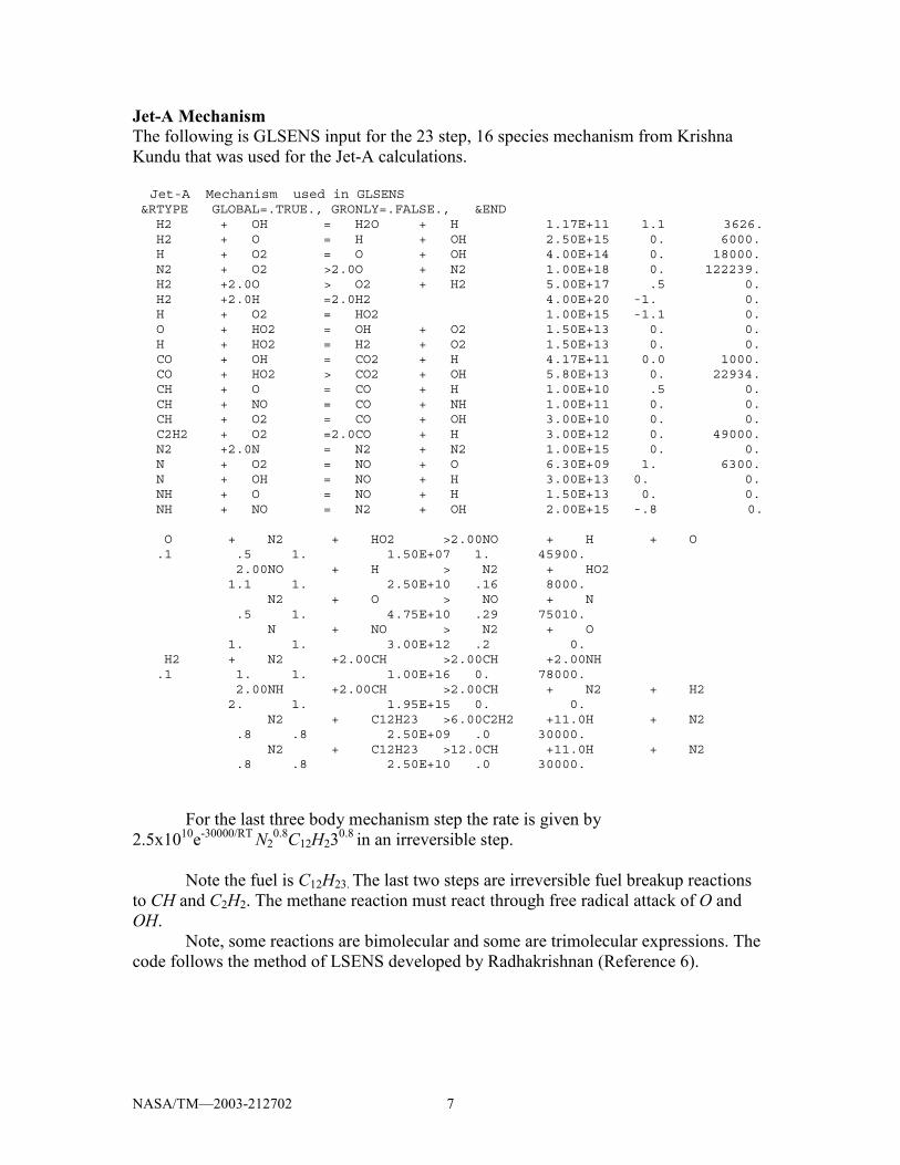
Jet-A Mechanism The following is GLSENS input for the 23 step, 16 species mechanism from Krishna Kundu that was used for the Jet-A calculations. Jet-A Mechanism used in GLSENS &RTYPE GLOBAL=.TRUE., GRONLY=.FALSE., &END H2 + OH = H2O + H 1.17E+11 1.1 3626. H2 + O = H + OH 2.50E+15 0. 6000. H + O2 = O + OH 4.00E+14 0. 18000. N2 + O2 >2.0O + N2 1.00E+18 0. 122239. H2 +2.0O > O2 + H2 5.00E+17 .5 0. H2 +2.0H =2.0H2 4.00E+20 -1. 0. H + O2 = HO2 1.00E+15 -1.1 0. O + HO2 = OH + O2 1.50E+13 0. 0. H + HO2 = H2 + O2 1.50E+13 0. 0. CO + OH = CO2 + H 4.17E+11 0.0 1000. CO + HO2 > CO2 + OH 5.80E+13 0. 22934. CH + O = CO + H 1.00E+10 .5 0. CH + NO = CO + NH 1.00E+11 0. 0. CH + O2 = CO + OH 3.00E+10 0. 0. C2H2 + O2 =2.0CO + H 3.00E+12 0. 49000. N2 +2.0N = N2 + N2 1.00E+15 0. 0. N + O2 = NO + O 6.30E+09 1. 6300. N + OH = NO + H 3.00E+13 0. 0. NH + O = NO + H 1.50E+13 0. 0. NH + NO = N2 + OH 2.00E+15 -.8 0. O + N2 + HO2 >2.00NO + H + O .1 .5 1. 1.50E+07 1. 45900. 2.00NO + H > N2 + HO2 1.1 1. 2.50E+10 .16 8000. N2 + O > NO + N .5 1. 4.75E+10 .29 75010. N + NO > N2 + O 1. 1. 3.00E+12 .2 0. H2 + N2 +2.00CH >2.00CH +2.00NH .1 1. 1. 1.00E+16 0. 78000. 2.00NH +2.00CH >2.00CH + N2 + H2 2. 1. 1.95E+15 0. 0. N2 + C12H23 >6.00C2H2 +11.0H + N2 .8 .8 2.50E+09 .0 30000. N2 + C12H23 >12.0CH +11.0H + N2 .8 .8 2.50E+10 .0 30000.
For the last three body mechanism step the rate is given by 2.5x10¹⁰e-30000/RT N2
0.8C12H230.8 in an irreversible step.
Note the fuel is C12H23. The last two steps are irreversible fuel breakup reactions to CH and C2H2. The methane reaction must react through free radical attack of O and OH.
Note, some reactions are bimolecular and some are trimolecular expressions. The code follows the method of LSENS developed by Radhakrishnan (Reference 6).
NASA/TM�2003-212702 8
Jet-A Results
The chemical kinetic time equations for Jet-A fuel may be found in Table 3.
Table 3. Jet -A Chemical Kinetic Time Correlations Species Lean Rich
Fuel ]T
14446exp[(P)(f/a)3.17eτ 0.6780.2725fuel
−−= ]T
15586exp[0.639(P)0.596(f/a)53.48efuelτ −−=
CO ]T
9535exp[0.743(P)0.349)0.0591(f/aCOτ −−= ]T
8009exp[0.781(P)0.570)0.0654(f/aCOτ −−=
NOx ]T
27513exp[(P)786(f/a)τ 1.560.28NOx
−−= ]T
26288exp[(P)981(f/a)τ 1.610.372NOx
−−=
These correlations show that the chemical kinetic time decreases with increasing pressure, resulting in a faster reaction. Parity plots for each chemical kinetic time equation were generated to show how close the simple model value for the chemical kinetic time was to the expected value. These plots can be found in Figures 5-10. The fuel and NOx plots show a strong correlation, however there is a greater amount of scatter in the CO plots. Figures 11-13 show the break in the chemical kinetic time function at an equivalence ratio of one. Concentration versus time is plotted in Figures 14-19 at temperatures of 1500K and 2500K for equivalence ratios of 0.5, 1.0, and 1.5. These plots are a comparison of the concentration given by the full mechanism and the concentration calculated by using the simple models. There was a fairly smooth transition between the lean and rich sides of the reaction. Auto ignition times using the simple model and a given formula were calculated and compared. The auto ignition time for the simple model is based on the recommendation of reference 7, where the time required for ignition is for 5 percent of the fuel to react.
τt
oeFFuel−
= (11) If 95.0=
oFFuel then 051.0=τ
t and Fuelignitionautot τ05.0= . (12)
Note that τfuel decreases as f/a decreases. We used an f/a of 0.02 with the lean equation. The formula for calculating the auto ignition time for Jet-A (reference 8) is given by:
=⋅ −
RTeatmondsmilliP 15300exp4.3)sec( 3τ (13)
Figure 20, a plot of auto ignition time versus temperatures, shows that the auto ignition time given by the simple model is fairly close to the auto ignition time given by the accepted formula. The two curves intersect at approximately 900K and then separate.
NASA/TM�2003-212702 9
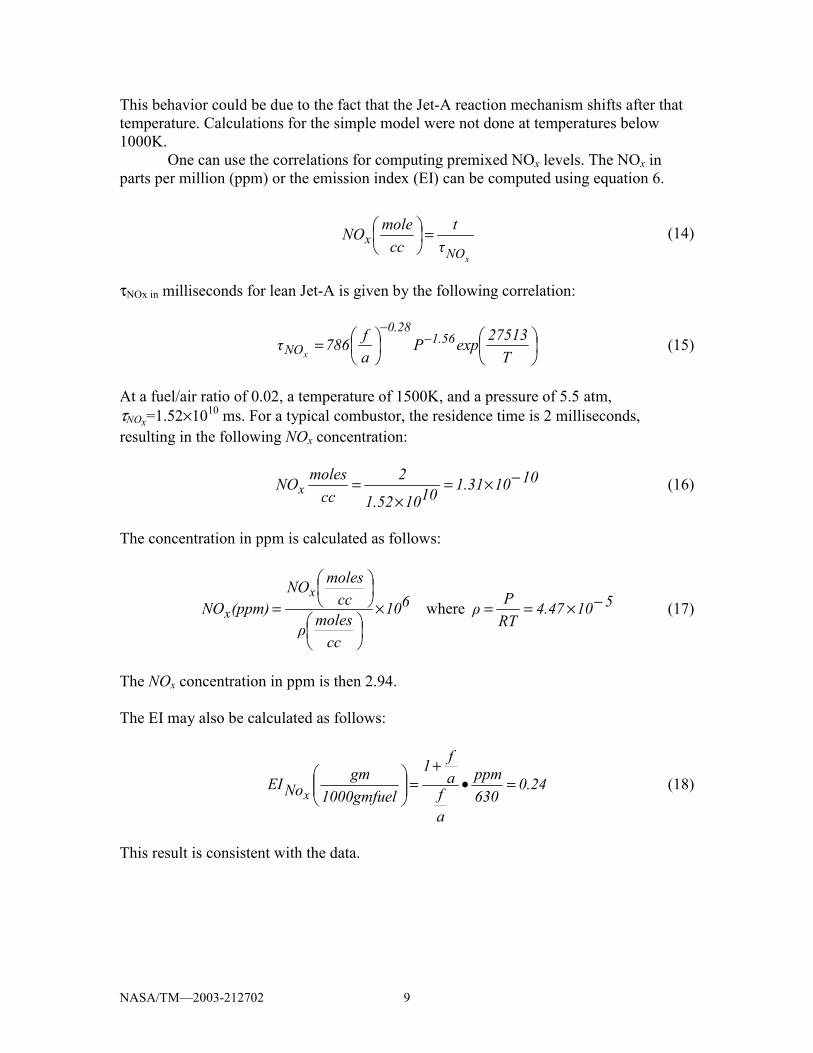
This behavior could be due to the fact that the Jet-A reaction mechanism shifts after that temperature. Calculations for the simple model were not done at temperatures below 1000K.
One can use the correlations for computing premixed NOx levels. The NOx in parts per million (ppm) or the emission index (EI) can be computed using equation 6.
(14) τNOx in milliseconds for lean Jet-A is given by the following correlation:
= −
−
T27513expP
af786τ 1.56
0.28
NOx (15)
At a fuel/air ratio of 0.02, a temperature of 1500K, and a pressure of 5.5 atm, τNOx=1.52×10¹⁰ ms. For a typical combustor, the residence time is 2 milliseconds, resulting in the following NOx concentration:
10101.3110101.52
2cc
molesNOx−×=
×= (16)
The concentration in ppm is calculated as follows:
610
ccmolesρ
ccmolesNO
(ppm)NOx
x ×
= where 5104.47RTPρ −×== (17)
The NOx concentration in ppm is then 2.94. The EI may also be calculated as follows:
0.24630ppm
af
af1
1000gmfuelgm
NoEIx
=•+
=
(18)
This result is consistent with the data.
xNOx τ
tcc
moleNO =
NASA/TM�2003-212702 10
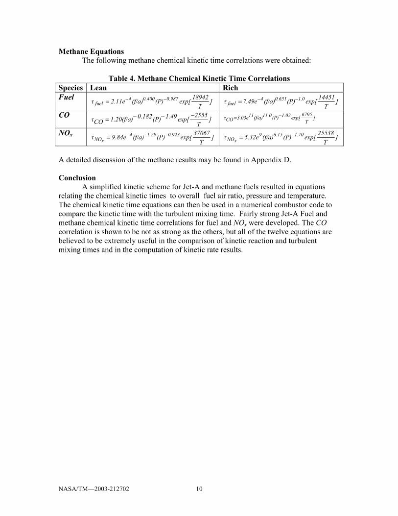
Methane Equations The following methane chemical kinetic time correlations were obtained:
Table 4. Methane Chemical Kinetic Time Correlations Species Lean Rich Fuel ]
T18942exp[(P)(f/a)2.11eτ 0.9870.4004
fuel−−= ]
T14451exp[(P)(f/a)7.49eτ 1.00.6514
fuel−−=
CO ]T
2555exp[1.49(P)0.1821.20(f/a)COτ −−−= ]T
6795exp[1.02(P)11.0(f/a)113.03eCOτ −=
NOx ]T
37067exp[(P)(f/a)9.84eτ 0.9231.294NOx
−−−= ]T
25538exp[(P)(f/a)5.32eτ 1.706.159NOx
−=
A detailed discussion of the methane results may be found in Appendix D. Conclusion
A simplified kinetic scheme for Jet-A and methane fuels resulted in equations relating the chemical kinetic times to overall fuel air ratio, pressure and temperature. The chemical kinetic time equations can then be used in a numerical combustor code to compare the kinetic time with the turbulent mixing time. Fairly strong Jet-A Fuel and methane chemical kinetic time correlations for fuel and NOx were developed. The CO correlation is shown to be not as strong as the others, but all of the twelve equations are believed to be extremely useful in the comparison of kinetic reaction and turbulent mixing times and in the computation of kinetic rate results.
NASA/TM�2003-212702 11
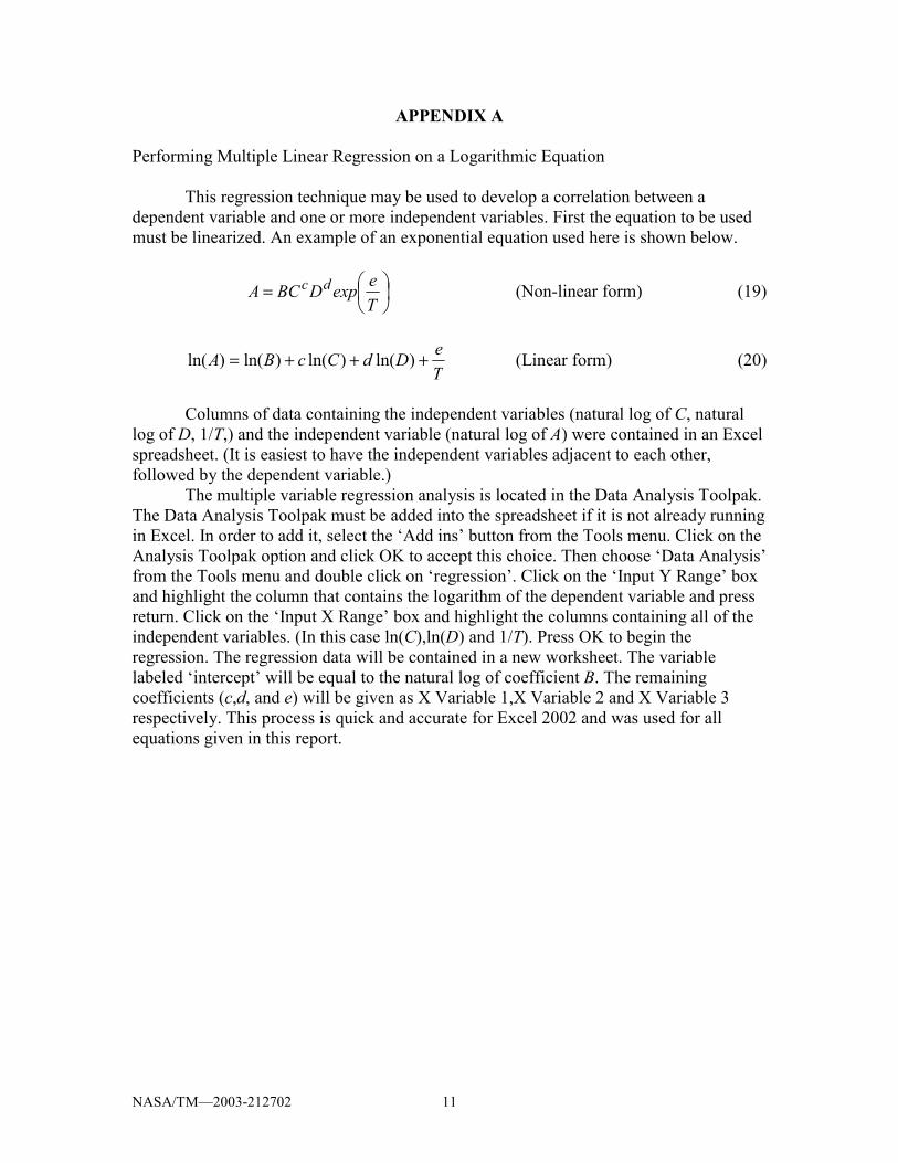
APPENDIX A Performing Multiple Linear Regression on a Logarithmic Equation
This regression technique may be used to develop a correlation between a dependent variable and one or more independent variables. First the equation to be used must be linearized. An example of an exponential equation used here is shown below.
=
TeexpDBCA dc (Non-linear form) (19)
TeDdCcBA +++= )ln()ln()ln()ln( (Linear form) (20)
Columns of data containing the independent variables (natural log of C, natural
log of D, 1/T,) and the independent variable (natural log of A) were contained in an Excel spreadsheet. (It is easiest to have the independent variables adjacent to each other, followed by the dependent variable.)
The multiple variable regression analysis is located in the Data Analysis Toolpak. The Data Analysis Toolpak must be added into the spreadsheet if it is not already running in Excel. In order to add it, select the �Add ins� button from the Tools menu. Click on the Analysis Toolpak option and click OK to accept this choice. Then choose �Data Analysis� from the Tools menu and double click on �regression�. Click on the �Input Y Range� box and highlight the column that contains the logarithm of the dependent variable and press return. Click on the �Input X Range� box and highlight the columns containing all of the independent variables. (In this case ln(C),ln(D) and 1/T). Press OK to begin the regression. The regression data will be contained in a new worksheet. The variable labeled �intercept� will be equal to the natural log of coefficient B. The remaining coefficients (c,d, and e) will be given as X Variable 1,X Variable 2 and X Variable 3 respectively. This process is quick and accurate for Excel 2002 and was used for all equations given in this report.

NASA/TM�2003-212702 13
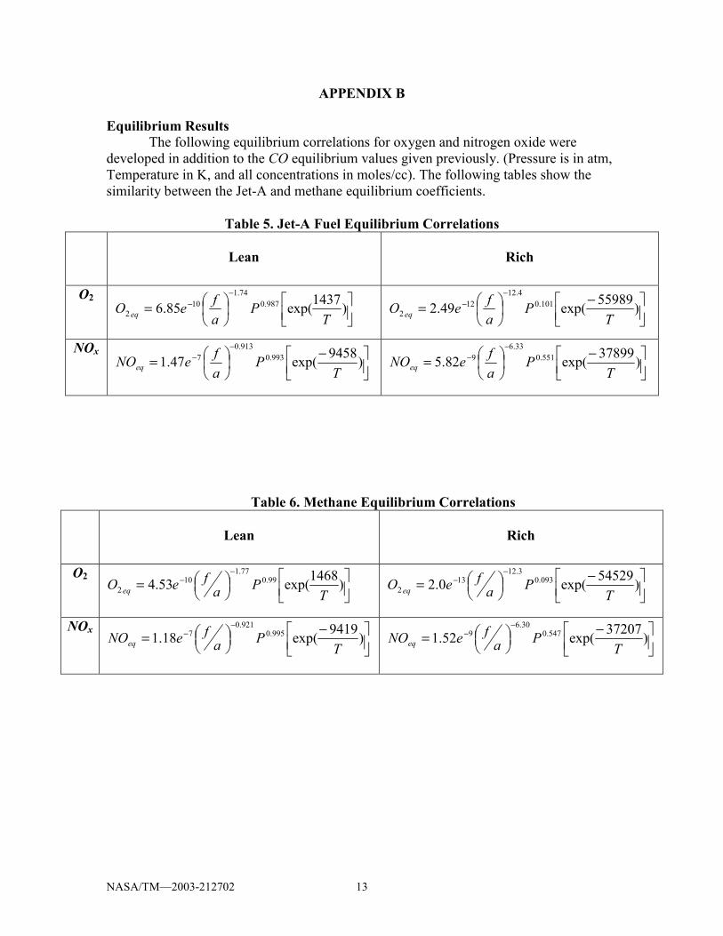
APPENDIX B Equilibrium Results
The following equilibrium correlations for oxygen and nitrogen oxide were developed in addition to the CO equilibrium values given previously. (Pressure is in atm, Temperature in K, and all concentrations in moles/cc). The following tables show the similarity between the Jet-A and methane equilibrium coefficients.
Table 5. Jet-A Fuel Equilibrium Correlations
Lean
Rich
O2
=
−− )1437exp(85.6 987.0
74.110
2 TP
afeO eq
−
=
−− )55989exp(49.2 101.0
4.1212
2 TP
afeO eq
NOx
−
=
−− )9458exp(47.1 993.0
913.07
TP
afeNOeq
−
=
−− )37899exp(82.5 551.0
33.69
TP
afeNOeq
Table 6. Methane Equilibrium Correlations
Lean
Rich
O2
=
−− )1468exp(53.4 99.0
77.110
2 TPa
feO eq
−
=
−− )54529exp(0.2 093.0
3.1213
2 TPa
feO eq
NOx
−
=
−− )9419exp(18.1 995.0
921.07
TPa
feNOeq
−
=
−− )37207exp(52.1 547.0
30.69
TPa
feNOeq

NASA/TM�2003-212702 15
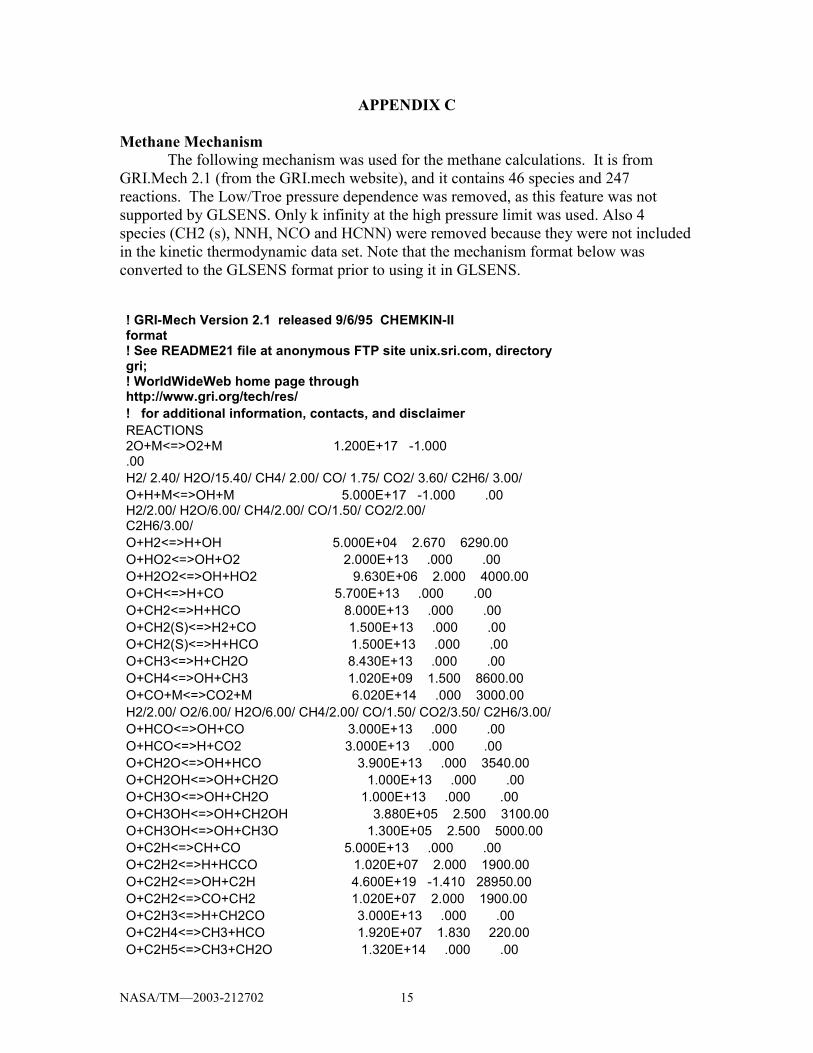
APPENDIX C Methane Mechanism
The following mechanism was used for the methane calculations. It is from GRI.Mech 2.1 (from the GRI.mech website), and it contains 46 species and 247 reactions. The Low/Troe pressure dependence was removed, as this feature was not supported by GLSENS. Only k infinity at the high pressure limit was used. Also 4 species (CH2 (s), NNH, NCO and HCNN) were removed because they were not included in the kinetic thermodynamic data set. Note that the mechanism format below was converted to the GLSENS format prior to using it in GLSENS. ! GRI-Mech Version 2.1 released 9/6/95 CHEMKIN-II format ! See README21 file at anonymous FTP site unix.sri.com, directory gri; ! WorldWideWeb home page through http://www.gri.org/tech/res/ ! for additional information, contacts, and disclaimer REACTIONS 2O+M<=>O2+M 1.200E+17 -1.000 .00 H2/ 2.40/ H2O/15.40/ CH4/ 2.00/ CO/ 1.75/ CO2/ 3.60/ C2H6/ 3.00/ O+H+M<=>OH+M 5.000E+17 -1.000 .00 H2/2.00/ H2O/6.00/ CH4/2.00/ CO/1.50/ CO2/2.00/ C2H6/3.00/ O+H2<=>H+OH 5.000E+04 2.670 6290.00 O+HO2<=>OH+O2 2.000E+13 .000 .00 O+H2O2<=>OH+HO2 9.630E+06 2.000 4000.00 O+CH<=>H+CO 5.700E+13 .000 .00 O+CH2<=>H+HCO 8.000E+13 .000 .00 O+CH2(S)<=>H2+CO 1.500E+13 .000 .00 O+CH2(S)<=>H+HCO 1.500E+13 .000 .00 O+CH3<=>H+CH2O 8.430E+13 .000 .00 O+CH4<=>OH+CH3 1.020E+09 1.500 8600.00 O+CO+M<=>CO2+M 6.020E+14 .000 3000.00 H2/2.00/ O2/6.00/ H2O/6.00/ CH4/2.00/ CO/1.50/ CO2/3.50/ C2H6/3.00/ O+HCO<=>OH+CO 3.000E+13 .000 .00 O+HCO<=>H+CO2 3.000E+13 .000 .00 O+CH2O<=>OH+HCO 3.900E+13 .000 3540.00 O+CH2OH<=>OH+CH2O 1.000E+13 .000 .00 O+CH3O<=>OH+CH2O 1.000E+13 .000 .00 O+CH3OH<=>OH+CH2OH 3.880E+05 2.500 3100.00 O+CH3OH<=>OH+CH3O 1.300E+05 2.500 5000.00 O+C2H<=>CH+CO 5.000E+13 .000 .00 O+C2H2<=>H+HCCO 1.020E+07 2.000 1900.00 O+C2H2<=>OH+C2H 4.600E+19 -1.410 28950.00 O+C2H2<=>CO+CH2 1.020E+07 2.000 1900.00 O+C2H3<=>H+CH2CO 3.000E+13 .000 .00 O+C2H4<=>CH3+HCO 1.920E+07 1.830 220.00 O+C2H5<=>CH3+CH2O 1.320E+14 .000 .00
NASA/TM�2003-212702 16
O+C2H6<=>OH+C2H5 8.980E+07 1.920 5690.00 O+HCCO<=>H+2CO 1.000E+14 .000 .00 O+CH2CO<=>OH+HCCO 1.000E+13 .000 8000.00 O+CH2CO<=>CH2+CO2 1.750E+12 .000 1350.00 O2+CO<=>O+CO2 2.500E+12 .000 47800.00 O2+CH2O<=>HO2+HCO 1.000E+14 .000 40000.00 H+O2+M<=>HO2+M 2.800E+18 -.860 .00 O2/ .00/ H2O/ .00/ CO/ .75/ CO2/1.50/ C2H6/1.50/ N2/ .00/ H+2O2<=>HO2+O2 3.000E+20 -1.720 .00 H+O2+H2O<=>HO2+H2O 9.380E+18 -.760 .00 H+O2+N2<=>HO2+N2 3.750E+20 -1.720 .00 H+O2<=>O+OH 8.300E+13 .000 14413.00 2H+M<=>H2+M 1.000E+18 -1.000 .00 H2/ .00/ H2O/ .00/ CH4/2.00/ CO2/ .00/ C2H6/3.00/ 2H+H2<=>2H2 9.000E+16 -.600 .00 2H+H2O<=>H2+H2O 6.000E+19 -1.250 .00 2H+CO2<=>H2+CO2 5.500E+20 -2.000 .00 H+OH+M<=>H2O+M 2.200E+22 -2.000 .00 H2/ .73/ H2O/3.65/ CH4/2.00/ C2H6/3.00/ H+HO2<=>O+H2O 3.970E+12 .000 671.00 H+HO2<=>O2+H2 2.800E+13 .000 1068.00 H+HO2<=>2OH 1.340E+14 .000 635.00 H+H2O2<=>HO2+H2 1.210E+07 2.000 5200.00 H+H2O2<=>OH+H2O 1.000E+13 .000 3600.00 H+CH<=>C+H2 1.100E+14 .000 .00 H+CH2(+M)<=>CH3(+M) 2.500E+16 -.800 .00 LOW / 3.200E+27 -3.140 1230.00/ TROE/ .6800 78.00 1995.00 5590.00 / H2/2.00/ H2O/6.00/ CH4/2.00/ CO/1.50/ CO2/2.00/ C2H6/3.00/ H+CH2(S)<=>CH+H2 3.000E+13 .000 .00 H+CH3(+M)<=>CH4(+M) 1.270E+16 -.630 383.00 LOW / 2.477E+33 -4.760 2440.00/ TROE/ .7830 74.00 2941.00 6964.00 / H2/2.00/ H2O/6.00/ CH4/2.00/ CO/1.50/ CO2/2.00/ C2H6/3.00/ H+CH4<=>CH3+H2 6.600E+08 1.620 10840.00 H+HCO(+M)<=>CH2O(+M) 1.090E+12 .480 -260.00 LOW / 1.350E+24 -2.570 1425.00/ TROE/ .7824 271.00 2755.00 6570.00 / H2/2.00/ H2O/6.00/ CH4/2.00/ CO/1.50/ CO2/2.00/ C2H6/3.00/ H+HCO<=>H2+CO 7.340E+13 .000 .00 H+CH2O(+M)<=>CH2OH(+M) 5.400E+11 .454 3600.00 LOW / 1.270E+32 -4.820 6530.00/ TROE/ .7187 103.00 1291.00 4160.00 / H2/2.00/ H2O/6.00/ CH4/2.00/ CO/1.50/ CO2/2.00/ C2H6/3.00/ H+CH2O(+M)<=>CH3O(+M) 5.400E+11 .454 2600.00 LOW / 2.200E+30 -4.800 5560.00/ TROE/ .7580 94.00 1555.00 4200.00 /
NASA/TM�2003-212702 17
H2/2.00/ H2O/6.00/ CH4/2.00/ CO/1.50/ CO2/2.00/ C2H6/3.00/ H+CH2O<=>HCO+H2 2.300E+10 1.050 3275.00 H+CH2OH(+M)<=>CH3OH(+M) 1.800E+13 .000 .00 LOW / 3.000E+31 -4.800 3300.00/ TROE/ .7679 338.00 1812.00 5081.00 / H2/2.00/ H2O/6.00/ CH4/2.00/ CO/1.50/ CO2/2.00/ C2H6/3.00/ H+CH2OH<=>H2+CH2O 2.000E+13 .000 .00 H+CH2OH<=>OH+CH3 1.200E+13 .000 .00 H+CH2OH<=>CH2(S)+H2O 6.000E+12 .000 .00 H+CH3O(+M)<=>CH3OH(+M) 5.000E+13 .000 .00 LOW / 8.600E+28 -4.000 3025.00/ TROE/ .8902 144.00 2838.00 45569.00 / H2/2.00/ H2O/6.00/ CH4/2.00/ CO/1.50/ CO2/2.00/ C2H6/3.00/ H+CH3O<=>H+CH2OH 3.400E+06 1.600 .00 H+CH3O<=>H2+CH2O 2.000E+13 .000 .00 H+CH3O<=>OH+CH3 3.200E+13 .000 .00 H+CH3O<=>CH2(S)+H2O 1.600E+13 .000 .00 H+CH3OH<=>CH2OH+H2 1.700E+07 2.100 4870.00 H+CH3OH<=>CH3O+H2 4.200E+06 2.100 4870.00 H+C2H(+M)<=>C2H2(+M) 1.000E+17 -1.000 .00 LOW / 3.750E+33 -4.800 1900.00/ TROE/ .6464 132.00 1315.00 5566.00 / H2/2.00/ H2O/6.00/ CH4/2.00/ CO/1.50/ CO2/2.00/ C2H6/3.00/ H+C2H2(+M)<=>C2H3(+M) 5.600E+12 .000 2400.00 LOW / 3.800E+40 -7.270 7220.00/ TROE/ .7507 98.50 1302.00 4167.00 / H2/2.00/ H2O/6.00/ CH4/2.00/ CO/1.50/ CO2/2.00/ C2H6/3.00/ H+C2H3(+M)<=>C2H4(+M) 6.080E+12 .270 280.00 LOW / 1.400E+30 -3.860 3320.00/ TROE/ .7820 207.50 2663.00 6095.00 / H2/2.00/ H2O/6.00/ CH4/2.00/ CO/1.50/ CO2/2.00/ C2H6/3.00/ H+C2H3<=>H2+C2H2 3.000E+13 .000 .00 H+C2H4(+M)<=>C2H5(+M) 1.080E+12 .454 1820.00 LOW / 1.200E+42 -7.620 6970.00/ TROE/ .9753 210.00 984.00 4374.00 / H2/2.00/ H2O/6.00/ CH4/2.00/ CO/1.50/ CO2/2.00/ C2H6/3.00/ H+C2H4<=>C2H3+H2 1.325E+06 2.530 12240.00 H+C2H5(+M)<=>C2H6(+M) 5.210E+17 -.990 1580.00 LOW / 1.990E+41 -7.080 6685.00/ TROE/ .8422 125.00 2219.00 6882.00 / H2/2.00/ H2O/6.00/ CH4/2.00/ CO/1.50/ CO2/2.00/ C2H6/3.00/ H+C2H5<=>H2+C2H4 2.000E+12 .000 .00 H+C2H6<=>C2H5+H2 1.150E+08 1.900 7530.00 H+HCCO<=>CH2(S)+CO 1.000E+14 .000 .00
NASA/TM�2003-212702 18
H+CH2CO<=>HCCO+H2 5.000E+13 .000 8000.00 H+CH2CO<=>CH3+CO 1.130E+13 .000 3428.00 H+HCCOH<=>H+CH2CO 1.000E+13 .000 .00 H2+CO(+M)<=>CH2O(+M) 4.300E+07 1.500 79600.00 LOW / 5.070E+27 -3.420 84350.00/ TROE/ .9320 197.00 1540.00 10300.00 / H2/2.00/ H2O/6.00/ CH4/2.00/ CO/1.50/ CO2/2.00/ C2H6/3.00/ OH+H2<=>H+H2O 2.160E+08 1.510 3430.00 2OH(+M)<=>H2O2(+M) 7.400E+13 -.370 .00 LOW / 2.300E+18 -.900 -1700.00/ TROE/ .7346 94.00 1756.00 5182.00 / H2/2.00/ H2O/6.00/ CH4/2.00/ CO/1.50/ CO2/2.00/ C2H6/3.00/ 2OH<=>O+H2O 3.570E+04 2.400 -2110.00 OH+HO2<=>O2+H2O 2.900E+13 .000 -500.00 OH+H2O2<=>HO2+H2O 1.750E+12 .000 320.00 DUPLICATE OH+H2O2<=>HO2+H2O 5.800E+14 .000 9560.00 DUPLICATE OH+C<=>H+CO 5.000E+13 .000 .00 OH+CH<=>H+HCO 3.000E+13 .000 .00 OH+CH2<=>H+CH2O 2.000E+13 .000 .00 OH+CH2<=>CH+H2O 1.130E+07 2.000 3000.00 OH+CH2(S)<=>H+CH2O 3.000E+13 .000 .00 OH+CH3(+M)<=>CH3OH(+M) 6.300E+13 .000 .00 LOW / 2.700E+38 -6.300 3100.00/ TROE/ .2105 83.50 5398.00 8370.00 / H2/2.00/ H2O/6.00/ CH4/2.00/ CO/1.50/ CO2/2.00/ C2H6/3.00/ OH+CH3<=>CH2+H2O 5.600E+07 1.600 5420.00 OH+CH3<=>CH2(S)+H2O 2.501E+13 .000 .00 OH+CH4<=>CH3+H2O 1.000E+08 1.600 3120.00 OH+CO<=>H+CO2 4.760E+07 1.228 70.00 OH+HCO<=>H2O+CO 5.000E+13 .000 .00 OH+CH2O<=>HCO+H2O 3.430E+09 1.180 -447.00 OH+CH2OH<=>H2O+CH2O 5.000E+12 .000 .00 OH+CH3O<=>H2O+CH2O 5.000E+12 .000 .00 OH+CH3OH<=>CH2OH+H2O 1.440E+06 2.000 -840.00 OH+CH3OH<=>CH3O+H2O 6.300E+06 2.000 1500.00 OH+C2H<=>H+HCCO 2.000E+13 .000 .00 OH+C2H2<=>H+CH2CO 2.180E-04 4.500 -1000.00 OH+C2H2<=>H+HCCOH 5.040E+05 2.300 13500.00 OH+C2H2<=>C2H+H2O 3.370E+07 2.000 14000.00 OH+C2H2<=>CH3+CO 4.830E-04 4.000 -2000.00 OH+C2H3<=>H2O+C2H2 5.000E+12 .000 .00 OH+C2H4<=>C2H3+H2O 3.600E+06 2.000 2500.00 OH+C2H6<=>C2H5+H2O 3.540E+06 2.120 870.00 OH+CH2CO<=>HCCO+H2O 7.500E+12 .000 2000.00 2HO2<=>O2+H2O2 1.300E+11 .000 -1630.00 DUPLICATE
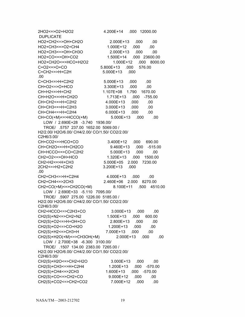
NASA/TM�2003-212702 19
2HO2<=>O2+H2O2 4.200E+14 .000 12000.00 DUPLICATE HO2+CH2<=>OH+CH2O 2.000E+13 .000 .00 HO2+CH3<=>O2+CH4 1.000E+12 .000 .00 HO2+CH3<=>OH+CH3O 2.000E+13 .000 .00 HO2+CO<=>OH+CO2 1.500E+14 .000 23600.00 HO2+CH2O<=>HCO+H2O2 1.000E+12 .000 8000.00 C+O2<=>O+CO 5.800E+13 .000 576.00 C+CH2<=>H+C2H 5.000E+13 .000 .00 C+CH3<=>H+C2H2 5.000E+13 .000 .00 CH+O2<=>O+HCO 3.300E+13 .000 .00 CH+H2<=>H+CH2 1.107E+08 1.790 1670.00 CH+H2O<=>H+CH2O 1.713E+13 .000 -755.00 CH+CH2<=>H+C2H2 4.000E+13 .000 .00 CH+CH3<=>H+C2H3 3.000E+13 .000 .00 CH+CH4<=>H+C2H4 6.000E+13 .000 .00 CH+CO(+M)<=>HCCO(+M) 5.000E+13 .000 .00 LOW / 2.690E+28 -3.740 1936.00/ TROE/ .5757 237.00 1652.00 5069.00 / H2/2.00/ H2O/6.00/ CH4/2.00/ CO/1.50/ CO2/2.00/ C2H6/3.00/ CH+CO2<=>HCO+CO 3.400E+12 .000 690.00 CH+CH2O<=>H+CH2CO 9.460E+13 .000 -515.00 CH+HCCO<=>CO+C2H2 5.000E+13 .000 .00 CH2+O2<=>OH+HCO 1.320E+13 .000 1500.00 CH2+H2<=>H+CH3 5.000E+05 2.000 7230.00 2CH2<=>H2+C2H2 3.200E+13 .000 .00 CH2+CH3<=>H+C2H4 4.000E+13 .000 .00 CH2+CH4<=>2CH3 2.460E+06 2.000 8270.00 CH2+CO(+M)<=>CH2CO(+M) 8.100E+11 .500 4510.00 LOW / 2.690E+33 -5.110 7095.00/ TROE/ .5907 275.00 1226.00 5185.00 / H2/2.00/ H2O/6.00/ CH4/2.00/ CO/1.50/ CO2/2.00/ C2H6/3.00/ CH2+HCCO<=>C2H3+CO 3.000E+13 .000 .00 CH2(S)+N2<=>CH2+N2 1.500E+13 .000 600.00 CH2(S)+O2<=>H+OH+CO 2.800E+13 .000 .00 CH2(S)+O2<=>CO+H2O 1.200E+13 .000 .00 CH2(S)+H2<=>CH3+H 7.000E+13 .000 .00 CH2(S)+H2O(+M)<=>CH3OH(+M) 2.000E+13 .000 .00 LOW / 2.700E+38 -6.300 3100.00/ TROE/ .1507 134.00 2383.00 7265.00 / H2/2.00/ H2O/6.00/ CH4/2.00/ CO/1.50/ CO2/2.00/ C2H6/3.00/ CH2(S)+H2O<=>CH2+H2O 3.000E+13 .000 .00 CH2(S)+CH3<=>H+C2H4 1.200E+13 .000 -570.00 CH2(S)+CH4<=>2CH3 1.600E+13 .000 -570.00 CH2(S)+CO<=>CH2+CO 9.000E+12 .000 .00 CH2(S)+CO2<=>CH2+CO2 7.000E+12 .000 .00
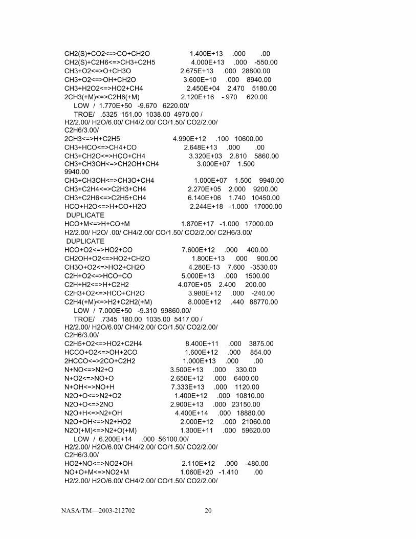
NASA/TM�2003-212702 20
CH2(S)+CO2<=>CO+CH2O 1.400E+13 .000 .00 CH2(S)+C2H6<=>CH3+C2H5 4.000E+13 .000 -550.00 CH3+O2<=>O+CH3O 2.675E+13 .000 28800.00 CH3+O2<=>OH+CH2O 3.600E+10 .000 8940.00 CH3+H2O2<=>HO2+CH4 2.450E+04 2.470 5180.00 2CH3(+M)<=>C2H6(+M) 2.120E+16 -.970 620.00 LOW / 1.770E+50 -9.670 6220.00/ TROE/ .5325 151.00 1038.00 4970.00 / H2/2.00/ H2O/6.00/ CH4/2.00/ CO/1.50/ CO2/2.00/ C2H6/3.00/ 2CH3<=>H+C2H5 4.990E+12 .100 10600.00 CH3+HCO<=>CH4+CO 2.648E+13 .000 .00 CH3+CH2O<=>HCO+CH4 3.320E+03 2.810 5860.00 CH3+CH3OH<=>CH2OH+CH4 3.000E+07 1.500 9940.00 CH3+CH3OH<=>CH3O+CH4 1.000E+07 1.500 9940.00 CH3+C2H4<=>C2H3+CH4 2.270E+05 2.000 9200.00 CH3+C2H6<=>C2H5+CH4 6.140E+06 1.740 10450.00 HCO+H2O<=>H+CO+H2O 2.244E+18 -1.000 17000.00 DUPLICATE HCO+M<=>H+CO+M 1.870E+17 -1.000 17000.00 H2/2.00/ H2O/ .00/ CH4/2.00/ CO/1.50/ CO2/2.00/ C2H6/3.00/ DUPLICATE HCO+O2<=>HO2+CO 7.600E+12 .000 400.00 CH2OH+O2<=>HO2+CH2O 1.800E+13 .000 900.00 CH3O+O2<=>HO2+CH2O 4.280E-13 7.600 -3530.00 C2H+O2<=>HCO+CO 5.000E+13 .000 1500.00 C2H+H2<=>H+C2H2 4.070E+05 2.400 200.00 C2H3+O2<=>HCO+CH2O 3.980E+12 .000 -240.00 C2H4(+M)<=>H2+C2H2(+M) 8.000E+12 .440 88770.00 LOW / 7.000E+50 -9.310 99860.00/ TROE/ .7345 180.00 1035.00 5417.00 / H2/2.00/ H2O/6.00/ CH4/2.00/ CO/1.50/ CO2/2.00/ C2H6/3.00/ C2H5+O2<=>HO2+C2H4 8.400E+11 .000 3875.00 HCCO+O2<=>OH+2CO 1.600E+12 .000 854.00 2HCCO<=>2CO+C2H2 1.000E+13 .000 .00 N+NO<=>N2+O 3.500E+13 .000 330.00 N+O2<=>NO+O 2.650E+12 .000 6400.00 N+OH<=>NO+H 7.333E+13 .000 1120.00 N2O+O<=>N2+O2 1.400E+12 .000 10810.00 N2O+O<=>2NO 2.900E+13 .000 23150.00 N2O+H<=>N2+OH 4.400E+14 .000 18880.00 N2O+OH<=>N2+HO2 2.000E+12 .000 21060.00 N2O(+M)<=>N2+O(+M) 1.300E+11 .000 59620.00 LOW / 6.200E+14 .000 56100.00/ H2/2.00/ H2O/6.00/ CH4/2.00/ CO/1.50/ CO2/2.00/ C2H6/3.00/ HO2+NO<=>NO2+OH 2.110E+12 .000 -480.00 NO+O+M<=>NO2+M 1.060E+20 -1.410 .00 H2/2.00/ H2O/6.00/ CH4/2.00/ CO/1.50/ CO2/2.00/
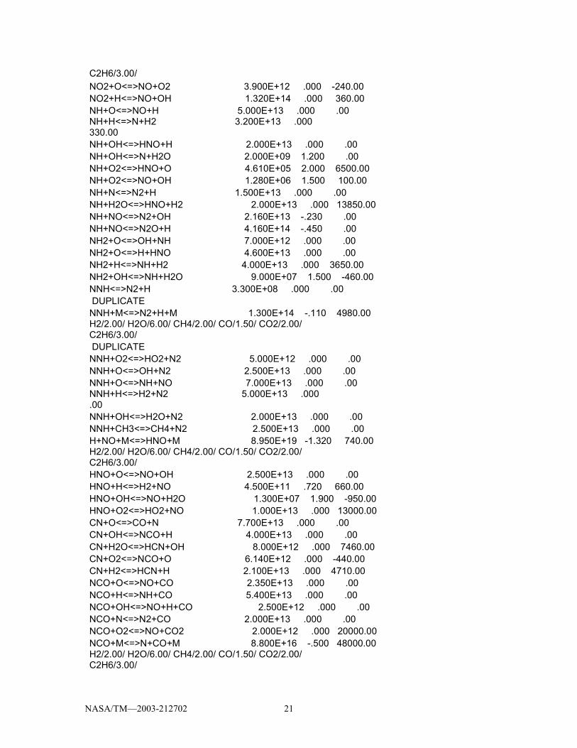
NASA/TM�2003-212702 21
C2H6/3.00/ NO2+O<=>NO+O2 3.900E+12 .000 -240.00 NO2+H<=>NO+OH 1.320E+14 .000 360.00 NH+O<=>NO+H 5.000E+13 .000 .00 NH+H<=>N+H2 3.200E+13 .000 330.00 NH+OH<=>HNO+H 2.000E+13 .000 .00 NH+OH<=>N+H2O 2.000E+09 1.200 .00 NH+O2<=>HNO+O 4.610E+05 2.000 6500.00 NH+O2<=>NO+OH 1.280E+06 1.500 100.00 NH+N<=>N2+H 1.500E+13 .000 .00 NH+H2O<=>HNO+H2 2.000E+13 .000 13850.00 NH+NO<=>N2+OH 2.160E+13 -.230 .00 NH+NO<=>N2O+H 4.160E+14 -.450 .00 NH2+O<=>OH+NH 7.000E+12 .000 .00 NH2+O<=>H+HNO 4.600E+13 .000 .00 NH2+H<=>NH+H2 4.000E+13 .000 3650.00 NH2+OH<=>NH+H2O 9.000E+07 1.500 -460.00 NNH<=>N2+H 3.300E+08 .000 .00 DUPLICATE NNH+M<=>N2+H+M 1.300E+14 -.110 4980.00 H2/2.00/ H2O/6.00/ CH4/2.00/ CO/1.50/ CO2/2.00/ C2H6/3.00/ DUPLICATE NNH+O2<=>HO2+N2 5.000E+12 .000 .00 NNH+O<=>OH+N2 2.500E+13 .000 .00 NNH+O<=>NH+NO 7.000E+13 .000 .00 NNH+H<=>H2+N2 5.000E+13 .000 .00 NNH+OH<=>H2O+N2 2.000E+13 .000 .00 NNH+CH3<=>CH4+N2 2.500E+13 .000 .00 H+NO+M<=>HNO+M 8.950E+19 -1.320 740.00 H2/2.00/ H2O/6.00/ CH4/2.00/ CO/1.50/ CO2/2.00/ C2H6/3.00/ HNO+O<=>NO+OH 2.500E+13 .000 .00 HNO+H<=>H2+NO 4.500E+11 .720 660.00 HNO+OH<=>NO+H2O 1.300E+07 1.900 -950.00 HNO+O2<=>HO2+NO 1.000E+13 .000 13000.00 CN+O<=>CO+N 7.700E+13 .000 .00 CN+OH<=>NCO+H 4.000E+13 .000 .00 CN+H2O<=>HCN+OH 8.000E+12 .000 7460.00 CN+O2<=>NCO+O 6.140E+12 .000 -440.00 CN+H2<=>HCN+H 2.100E+13 .000 4710.00 NCO+O<=>NO+CO 2.350E+13 .000 .00 NCO+H<=>NH+CO 5.400E+13 .000 .00 NCO+OH<=>NO+H+CO 2.500E+12 .000 .00 NCO+N<=>N2+CO 2.000E+13 .000 .00 NCO+O2<=>NO+CO2 2.000E+12 .000 20000.00 NCO+M<=>N+CO+M 8.800E+16 -.500 48000.00 H2/2.00/ H2O/6.00/ CH4/2.00/ CO/1.50/ CO2/2.00/ C2H6/3.00/
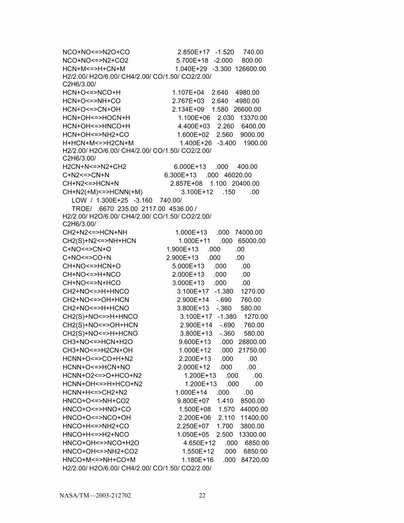
NASA/TM�2003-212702 22
NCO+NO<=>N2O+CO 2.850E+17 -1.520 740.00 NCO+NO<=>N2+CO2 5.700E+18 -2.000 800.00 HCN+M<=>H+CN+M 1.040E+29 -3.300 126600.00 H2/2.00/ H2O/6.00/ CH4/2.00/ CO/1.50/ CO2/2.00/ C2H6/3.00/ HCN+O<=>NCO+H 1.107E+04 2.640 4980.00 HCN+O<=>NH+CO 2.767E+03 2.640 4980.00 HCN+O<=>CN+OH 2.134E+09 1.580 26600.00 HCN+OH<=>HOCN+H 1.100E+06 2.030 13370.00 HCN+OH<=>HNCO+H 4.400E+03 2.260 6400.00 HCN+OH<=>NH2+CO 1.600E+02 2.560 9000.00 H+HCN+M<=>H2CN+M 1.400E+26 -3.400 1900.00 H2/2.00/ H2O/6.00/ CH4/2.00/ CO/1.50/ CO2/2.00/ C2H6/3.00/ H2CN+N<=>N2+CH2 6.000E+13 .000 400.00 C+N2<=>CN+N 6.300E+13 .000 46020.00 CH+N2<=>HCN+N 2.857E+08 1.100 20400.00 CH+N2(+M)<=>HCNN(+M) 3.100E+12 .150 .00 LOW / 1.300E+25 -3.160 740.00/ TROE/ .6670 235.00 2117.00 4536.00 / H2/2.00/ H2O/6.00/ CH4/2.00/ CO/1.50/ CO2/2.00/ C2H6/3.00/ CH2+N2<=>HCN+NH 1.000E+13 .000 74000.00 CH2(S)+N2<=>NH+HCN 1.000E+11 .000 65000.00 C+NO<=>CN+O 1.900E+13 .000 .00 C+NO<=>CO+N 2.900E+13 .000 .00 CH+NO<=>HCN+O 5.000E+13 .000 .00 CH+NO<=>H+NCO 2.000E+13 .000 .00 CH+NO<=>N+HCO 3.000E+13 .000 .00 CH2+NO<=>H+HNCO 3.100E+17 -1.380 1270.00 CH2+NO<=>OH+HCN 2.900E+14 -.690 760.00 CH2+NO<=>H+HCNO 3.800E+13 -.360 580.00 CH2(S)+NO<=>H+HNCO 3.100E+17 -1.380 1270.00 CH2(S)+NO<=>OH+HCN 2.900E+14 -.690 760.00 CH2(S)+NO<=>H+HCNO 3.800E+13 -.360 580.00 CH3+NO<=>HCN+H2O 9.600E+13 .000 28800.00 CH3+NO<=>H2CN+OH 1.000E+12 .000 21750.00 HCNN+O<=>CO+H+N2 2.200E+13 .000 .00 HCNN+O<=>HCN+NO 2.000E+12 .000 .00 HCNN+O2<=>O+HCO+N2 1.200E+13 .000 .00 HCNN+OH<=>H+HCO+N2 1.200E+13 .000 .00 HCNN+H<=>CH2+N2 1.000E+14 .000 .00 HNCO+O<=>NH+CO2 9.800E+07 1.410 8500.00 HNCO+O<=>HNO+CO 1.500E+08 1.570 44000.00 HNCO+O<=>NCO+OH 2.200E+06 2.110 11400.00 HNCO+H<=>NH2+CO 2.250E+07 1.700 3800.00 HNCO+H<=>H2+NCO 1.050E+05 2.500 13300.00 HNCO+OH<=>NCO+H2O 4.650E+12 .000 6850.00 HNCO+OH<=>NH2+CO2 1.550E+12 .000 6850.00 HNCO+M<=>NH+CO+M 1.180E+16 .000 84720.00 H2/2.00/ H2O/6.00/ CH4/2.00/ CO/1.50/ CO2/2.00/
NASA/TM�2003-212702 23
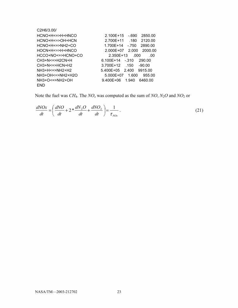
C2H6/3.00/ HCNO+H<=>H+HNCO 2.100E+15 -.690 2850.00 HCNO+H<=>OH+HCN 2.700E+11 .180 2120.00 HCNO+H<=>NH2+CO 1.700E+14 -.750 2890.00 HOCN+H<=>H+HNCO 2.000E+07 2.000 2000.00 HCCO+NO<=>HCNO+CO 2.350E+13 .000 .00 CH3+N<=>H2CN+H 6.100E+14 -.310 290.00 CH3+N<=>HCN+H2 3.700E+12 .150 -90.00 NH3+H<=>NH2+H2 5.400E+05 2.400 9915.00 NH3+OH<=>NH2+H2O 5.000E+07 1.600 955.00 NH3+O<=>NH2+OH 9.400E+06 1.940 6460.00 END
Note the fuel was CH4. The NOx was computed as the sum of NO, N2O and NO2 or
NOxdtdNO
dtOdN
dtdNO
dtdNOx
τ1*2 22 =
++= . (21)

NASA/TM�2003-212702 25
APPENDIX D Methane Results Figures 21 and 22 are parity plots showing the strength of the lean and rich equilibrium correlations for CO. These charts show very strong CO equilibrium correlations for methane, similar to those for the Jet-A fuel.
The chemical kinetic time correlations developed for methane may be found in Table (4). Parity plots for the chemical kinetic times are given in Figures 23-28. Values on the x-axis represent chemical kinetic times in milliseconds calculated in GLSENS using the complete mechanism, and values on the y-axis represent chemical kinetic times calculated by this report�s simple model. The fuel and NOx parity plots show a fairly tight fitting curve, with a minimal amount of scattering. The CO parity plots show a larger amount of scattering. However, the resulting correlations are still believed to be useful in calculating the chemical kinetic times at various sets of conditions.

NASA/TM�2003-212702 27
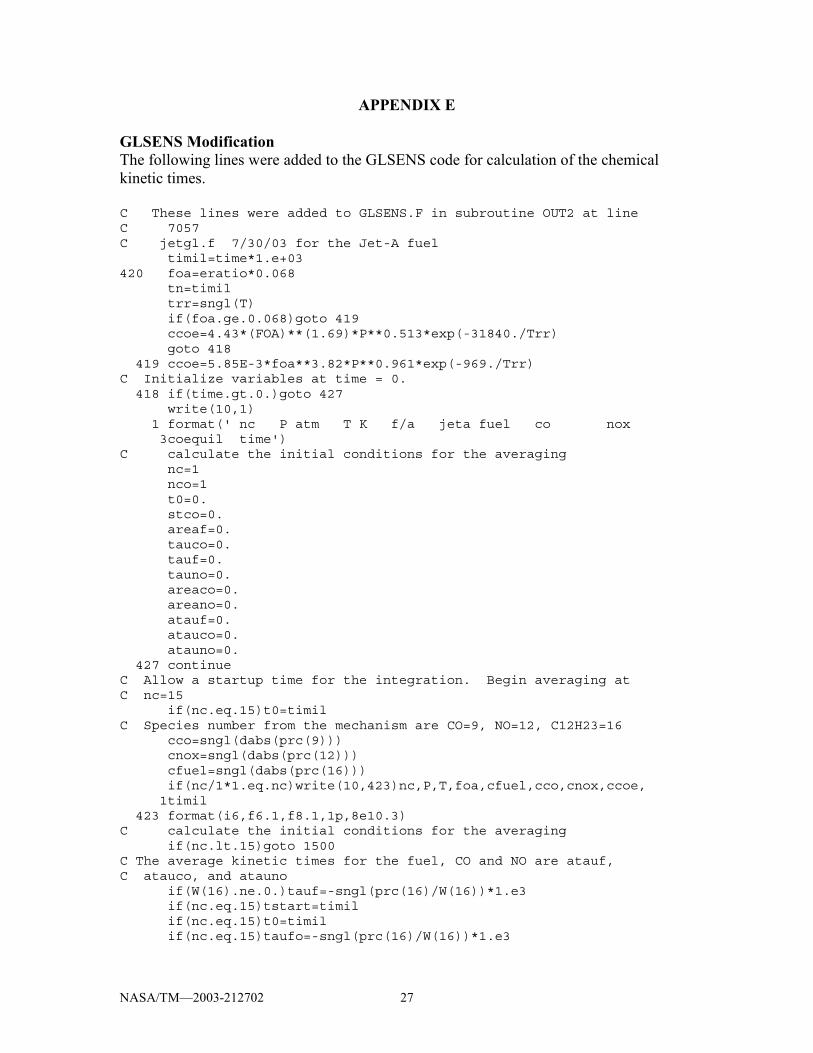
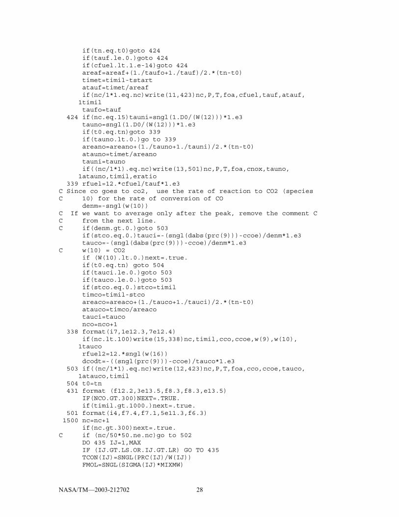
APPENDIX E GLSENS Modification The following lines were added to the GLSENS code for calculation of the chemical kinetic times. C These lines were added to GLSENS.F in subroutine OUT2 at line C 7057 C jetgl.f 7/30/03 for the Jet-A fuel timil=time*1.e+03 420 foa=eratio*0.068 tn=timil trr=sngl(T) if(foa.ge.0.068)goto 419 ccoe=4.43*(FOA)**(1.69)*P**0.513*exp(-31840./Trr) goto 418 419 ccoe=5.85E-3*foa**3.82*P**0.961*exp(-969./Trr) C Initialize variables at time = 0. 418 if(time.gt.0.)goto 427 write(10,1) 1 format(' nc P atm T K f/a jeta fuel co nox 3coequil time') C calculate the initial conditions for the averaging nc=1 nco=1 t0=0. stco=0. areaf=0. tauco=0. tauf=0. tauno=0. areaco=0. areano=0. atauf=0. atauco=0. atauno=0. 427 continue C Allow a startup time for the integration. Begin averaging at C nc=15 if(nc.eq.15)t0=timil C Species number from the mechanism are CO=9, NO=12, C12H23=16 cco=sngl(dabs(prc(9))) cnox=sngl(dabs(prc(12))) cfuel=sngl(dabs(prc(16))) if(nc/1*1.eq.nc)write(10,423)nc,P,T,foa,cfuel,cco,cnox,ccoe, 1timil 423 format(i6,f6.1,f8.1,1p,8e10.3) C calculate the initial conditions for the averaging if(nc.lt.15)goto 1500 C The average kinetic times for the fuel, CO and NO are atauf, C atauco, and atauno if(W(16).ne.0.)tauf=-sngl(prc(16)/W(16))*1.e3 if(nc.eq.15)tstart=timil if(nc.eq.15)t0=timil if(nc.eq.15)taufo=-sngl(prc(16)/W(16))*1.e3
NASA/TM�2003-212702 28
if(tn.eq.t0)goto 424 if(tauf.le.0.)goto 424 if(cfuel.lt.1.e-14)goto 424 areaf=areaf+(1./taufo+1./tauf)/2.*(tn-t0) timet=timil-tstart atauf=timet/areaf if(nc/1*1.eq.nc)write(11,423)nc,P,T,foa,cfuel,tauf,atauf, 1timil taufo=tauf 424 if(nc.eq.15)tauni=sngl(1.D0/(W(12)))*1.e3 tauno=sngl(1.D0/(W(12)))*1.e3 if(t0.eq.tn)goto 339 if(tauno.lt.0.)go to 339 areano=areano+(1./tauno+1./tauni)/2.*(tn-t0) atauno=timet/areano tauni=tauno if((nc/1*1).eq.nc)write(13,501)nc,P,T,foa,cnox,tauno, 1atauno,timil,eratio 339 rfuel=12.*cfuel/tauf*1.e3 C Since co goes to co2, use the rate of reaction to CO2 (species C 10) for the rate of conversion of CO denm=-sngl(w(10)) C If we want to average only after the peak, remove the comment C C from the next line. C if(denm.gt.0.)goto 503 if(stco.eq.0.)tauci=-(sngl(dabs(prc(9)))-ccoe)/denm*1.e3 tauco=-(sngl(dabs(prc(9)))-ccoe)/denm*1.e3 C w(10) = CO2 if (W(10).lt.0.)next=.true. if(t0.eq.tn) goto 504 if(tauci.le.0.)goto 503 if(tauco.le.0.)goto 503 if(stco.eq.0.)stco=timil timco=timil-stco areaco=areaco+(1./tauco+1./tauci)/2.*(tn-t0) atauco=timco/areaco tauci=tauco nco=nco+1 338 format(i7,1e12.3,7e12.4) if(nc.lt.100)write(15,338)nc,timil,cco,ccoe,w(9),w(10), 1tauco rfuel2=12.*sngl(w(16)) dcodt=-((sngl(prc(9)))-ccoe)/tauco*1.e3 503 if((nc/1*1).eq.nc)write(12,423)nc,P,T,foa,cco,ccoe,tauco, 1atauco,timil 504 t0=tn 431 format (f12.2,3e13.5,f8.3,f8.3,e13.5) IF(NCO.GT.300)NEXT=.TRUE. if(timil.gt.1000.)next=.true. 501 format(i4,f7.4,f7.1,5e11.3,f6.3) 1500 nc=nc+1 if(nc.gt.300)next=.true. C if (nc/50*50.ne.nc)go to 502 DO 435 IJ=1,MAX IF (IJ.GT.LS.OR.IJ.GT.LR) GO TO 435 TCON(IJ)=SNGL(PRC(IJ)/W(IJ)) FMOL=SNGL(SIGMA(IJ)*MIXMW)
NASA/TM�2003-212702 29
WRITE (LWRITE,175) DSPNM(IJ),PRC(IJ),FMOL,W(IJ) GO TO 435 430 WRITE (LWRITE,185) IJ,RATE(IJ),PRX(IJ),EQUIL(IJ) C430 continue 435 CONTINUE C The variables atauf, atauco and atauno are saved in a common C block and printed in main after the completion of the complete C time integration as ln(foa), ln(p), 1./T, Ln(atauf), C ln(atauco), and ln(atauno) for processing by Excel regression 502 IF (WELSTR) GO TO 446 C WRITE (LWRITE,440) DSNAM(1),FF(LSP1),DSNAM(2),FF(LSP2) 440 FORMAT (/,4X,'DERIVATIVES (CGS UNITS): ',2(A8,4X,1PE12.5,4X))

NASA/TM�2003-212702 31
REFERENCES 1. Brink, Anders; Mueller, Christian; Kilpinen, Pia and Hupa, Mikko: Possibilities and
Limitations of the Eddy Break-Up Model, Combustion and Flame, 123, 275�279 (2000)
2. Penko, P.F.; Kundu, K.P.; Siow, Y.K.; and Yang, S.L.: A Kinetic Mechanism for Calculation of Pollutant Species in Jet-A Combustion, AIAA 2000�3035
3. Kundu, K.P.; Penko, P.F.; and VanOverbeke, T.J.: A Practical Mechanism for Computing Combustion in Gas Turbine Engines, AIAA 99�2218
4. Bittker, D.A., GLSENS, A Generalized Extension of LSENS Including Global Reactions and Added Sensitivity Analysis for the Perfectly Stirred Reactor, NASA Reference Publication 1362, 1999.
5. Sanford, Gordon; and McBride, Bonnie J., Computer Program for Calculation of Complex Chemical Equilibrium Composition and Applications, NASA Reference Publication 1311, October 1994.
6. Radhakrishnan, Krishnan; and Bittker, David A., LSENS, A General Chemical Kinetics and Sensitivity Analysis Code for Homogeneous Gas-Phase Reactions, NASA Reference Publication 1329.
7. Huber, Paul W.; Schexnayder, Jr., Charles J.; and McClinton, Charles R.: Criteria for Self-Ignition of Supersonic Hydrogen-Air Mixtures, NASA TP�1457, 1979.
8. Marek, Cecil J.; and Baker, Charles E.: High-Pressure Flame Visualization of Autoignition and Flashback Phenomena With a Liquid-Fuel Spray. NASA TM�83501, October 1983.

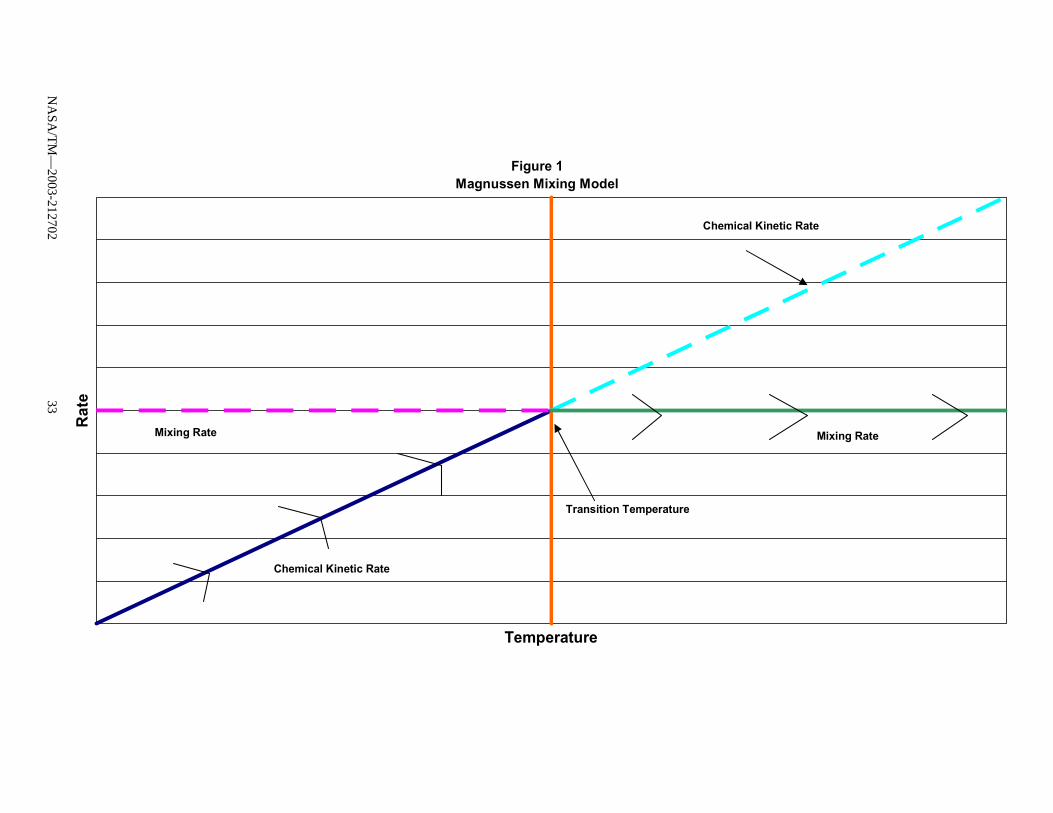
Figure 1 Magnussen Mixing Model
Temperature
Rat
e
Chemical Kinetic Rate
Mixing Rate
Transition Temperature
Mixing Rate
Chemical Kinetic Rate
NA
SA/T
M—
2003-21270233
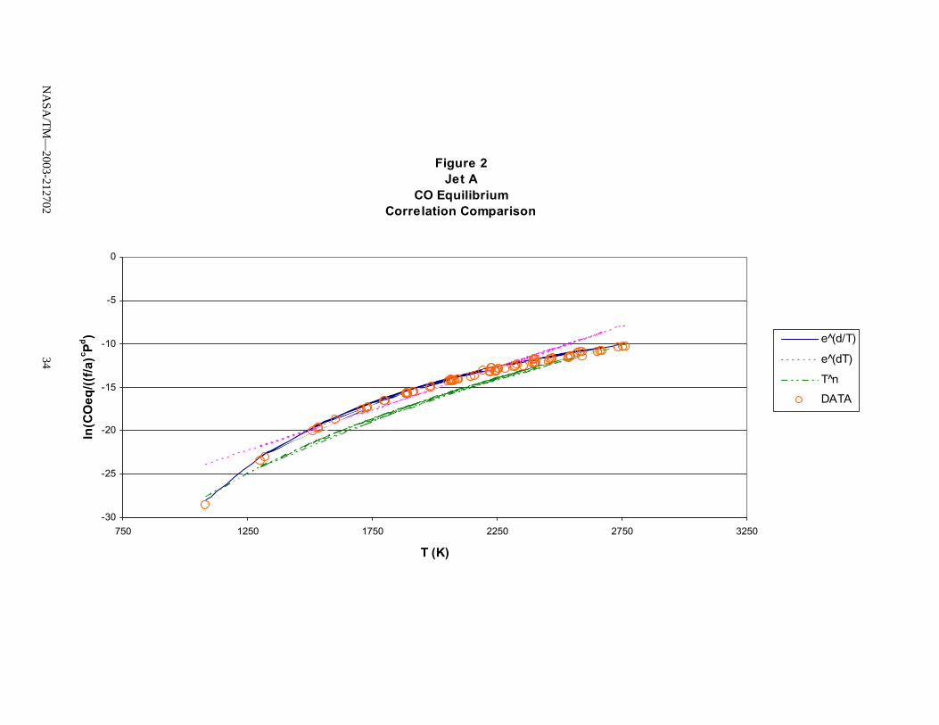
Figure 2 Jet A
CO EquilibriumCorrelation Comparison
-30
-25
-20
-15
-10
-5
0
750 1250 1750 2250 2750 3250
T (K)
ln(C
Oeq
/((f/a
)c Pd ) e (̂d/T)
e (̂dT)
T n̂
DATA
NA
SA/T
M—
2003-21270234
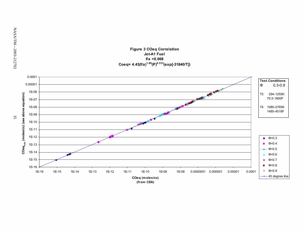
Figure 3 COeq CorrelationJet-A1 Fuelf/a <0.068
Coeq= 4.43(f/a)1.69(P)0.513(exp[-31840/T])
1E-16
1E-15
1E-14
1E-13
1E-12
1E-11
1E-10
1E-09
1E-08
1E-07
1E-06
0.00001
0.0001
1E-16 1E-15 1E-14 1E-13 1E-12 1E-11 1E-10 1E-09 1E-08 0.0000001 0.000001 0.00001 0.0001
COeq (moles/cc)(from CEA)
CO
eqca
lc (m
oles
/cc)
(see
abo
ve e
quat
ion)
Φ=0.3
Φ=0.4
Φ=0.5
Φ=0.6
Φ=0.7
Φ=0.8
Φ=0.9
45 degree line
Test ConditionsΦ 0.3-0.9
T3 294-1255K 70.5-1800F
T4 1080-2765K 1485-4518F
NA
SA/T
M—
2003-21270235
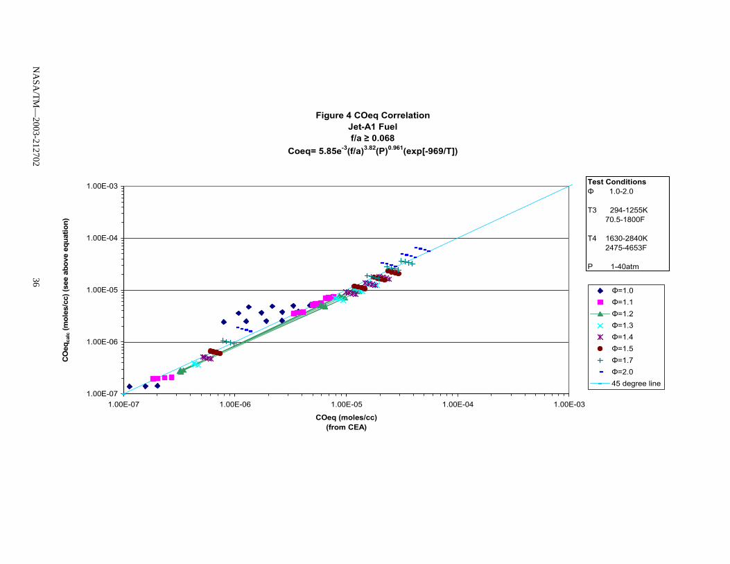
Figure 4 COeq CorrelationJet-A1 Fuelf/a ≥ 0.068
Coeq= 5.85e-3(f/a)3.82(P)0.961(exp[-969/T])
1.00E-07
1.00E-06
1.00E-05
1.00E-04
1.00E-03
1.00E-07 1.00E-06 1.00E-05 1.00E-04 1.00E-03
COeq (moles/cc) (from CEA)
CO
eqca
lc (m
oles
/cc)
(see
abo
ve e
quat
ion)
Φ=1.0Φ=1.1Φ=1.2Φ=1.3Φ=1.4Φ=1.5Φ=1.7Φ=2.045 degree line
Test ConditionsΦ 1.0-2.0
T3 294-1255K 70.5-1800F
T4 1630-2840K 2475-4653F
P 1-40atm
NA
SA/T
M—
2003-21270236
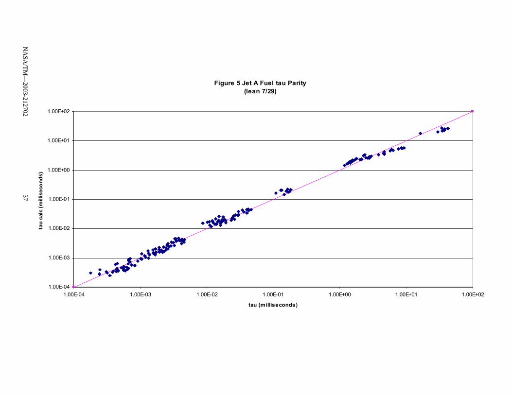
Figure 5 Jet A Fuel tau Parity (lean 7/29)
1.00E-04
1.00E-03
1.00E-02
1.00E-01
1.00E+00
1.00E+01
1.00E+02
1.00E-04 1.00E-03 1.00E-02 1.00E-01 1.00E+00 1.00E+01 1.00E+02
tau (milliseconds)
tau
calc
(mill
isec
onds
)
NA
SA/T
M—
2003-21270237
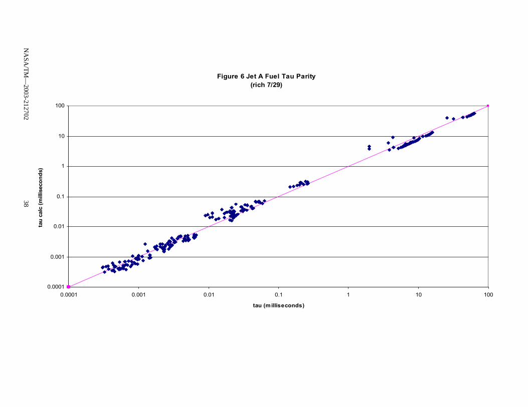
Figure 6 Jet A Fuel Tau Parity (rich 7/29)
0.0001
0.001
0.01
0.1
1
10
100
0.0001 0.001 0.01 0.1 1 10 100
tau (milliseconds)
tau
calc
(mill
isec
onds
)
NA
SA/T
M—
2003-21270238
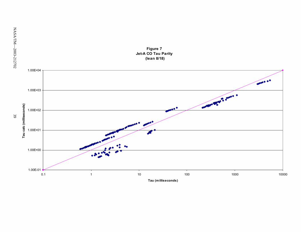
Figure 7Jet-A CO Tau Parity
(lean 8/18)
1.00E-01
1.00E+00
1.00E+01
1.00E+02
1.00E+03
1.00E+04
0.1 1 10 100 1000 10000
Tau (milliseconds)
Tau
calc
(mill
isec
onds
)
NA
SA/T
M—
2003-21270239
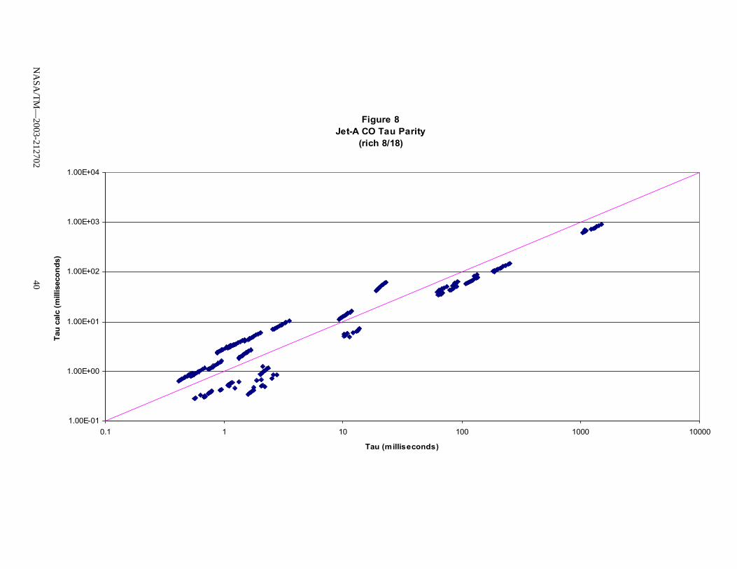
Figure 8Jet-A CO Tau Parity
(rich 8/18)
1.00E-01
1.00E+00
1.00E+01
1.00E+02
1.00E+03
1.00E+04
0.1 1 10 100 1000 10000
Tau (milliseconds)
Tau
calc
(mill
isec
onds
)
NA
SA/T
M—
2003-21270240
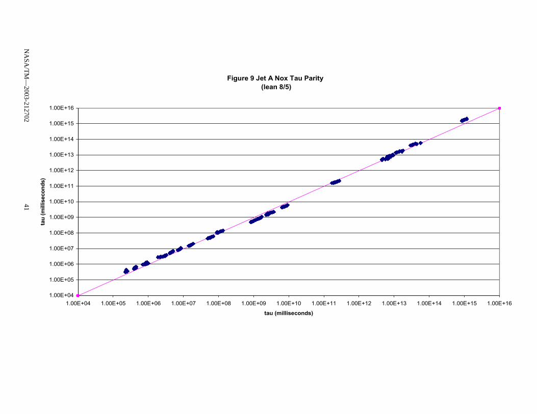
Figure 9 Jet A Nox Tau Parity (lean 8/5)
1.00E+04
1.00E+05
1.00E+06
1.00E+07
1.00E+08
1.00E+09
1.00E+10
1.00E+11
1.00E+12
1.00E+13
1.00E+14
1.00E+15
1.00E+16
1.00E+04 1.00E+05 1.00E+06 1.00E+07 1.00E+08 1.00E+09 1.00E+10 1.00E+11 1.00E+12 1.00E+13 1.00E+14 1.00E+15 1.00E+16
tau (milliseconds)
tau
(mill
isec
onds
)
NA
SA/T
M—
2003-21270241
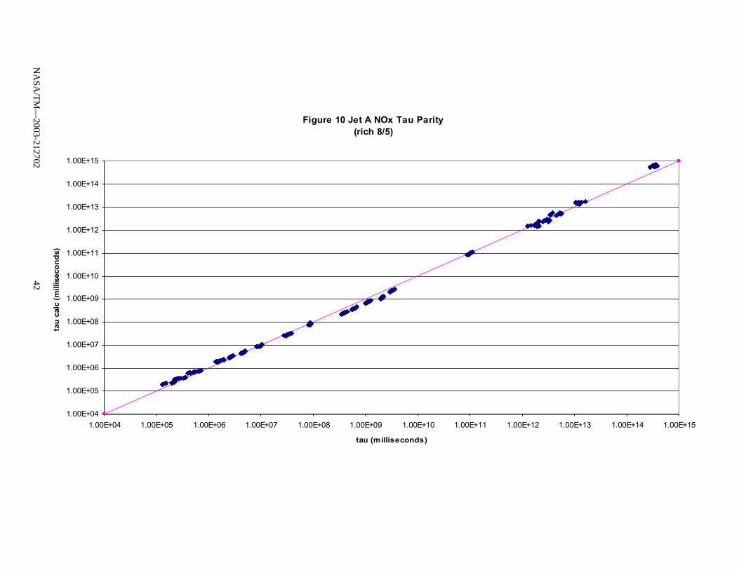
Figure 10 Jet A NOx Tau Parity (rich 8/5)
1.00E+04
1.00E+05
1.00E+06
1.00E+07
1.00E+08
1.00E+09
1.00E+10
1.00E+11
1.00E+12
1.00E+13
1.00E+14
1.00E+15
1.00E+04 1.00E+05 1.00E+06 1.00E+07 1.00E+08 1.00E+09 1.00E+10 1.00E+11 1.00E+12 1.00E+13 1.00E+14 1.00E+15
tau (milliseconds)
tau
calc
(mill
isec
onds
)
NA
SA/T
M—
2003-21270242
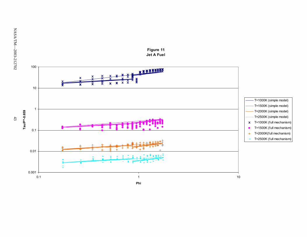
Figure 11 Jet A Fuel
0.001
0.01
0.1
1
10
100
0.1 1 10
Phi
Tau/
P-̂0
.659
T=1000K (simple model)
T=1500K (simple model)
T=2000K (simple model)
T=2500K (simple model)
T=1000K (full mechanism)
T=1500K (full mechanism)
T=2000K(full mechanism)
T=2500K (full mechanism)
NA
SA/T
M—
2003-21270243
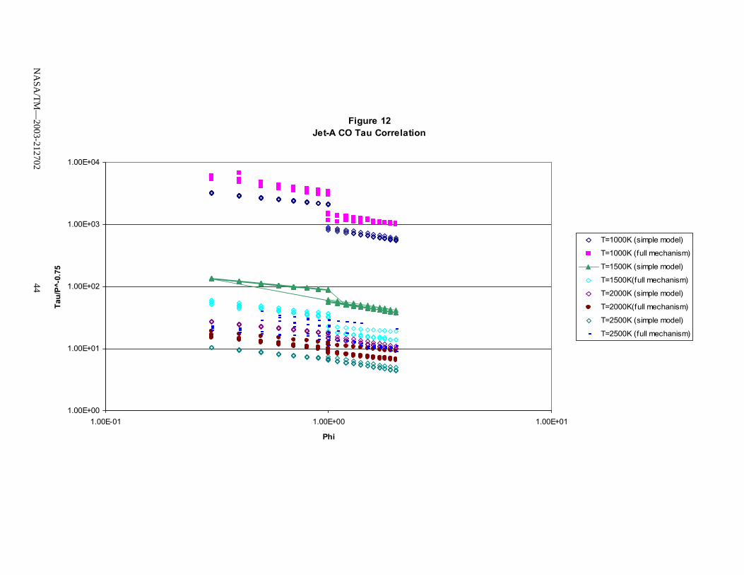
Figure 12Jet-A CO Tau Correlation
1.00E+00
1.00E+01
1.00E+02
1.00E+03
1.00E+04
1.00E-01 1.00E+00 1.00E+01
Phi
Tau/
P^-0
.75
T=1000K (simple model)
T=1000K (full mechanism)
T=1500K (simple model)
T=1500K(full mechanism)
T=2000K (simple model)
T=2000K(full mechanism)
T=2500K (simple model)
T=2500K (full mechanism)
NA
SA/T
M—
2003-21270244
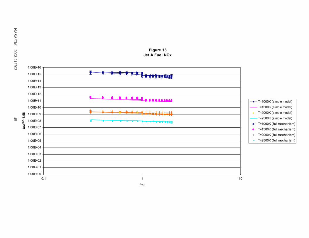
Figure 13Jet A Fuel NOx
1.00E+00
1.00E+01
1.00E+02
1.00E+03
1.00E+04
1.00E+05
1.00E+06
1.00E+07
1.00E+08
1.00E+09
1.00E+10
1.00E+11
1.00E+12
1.00E+13
1.00E+14
1.00E+15
1.00E+16
0.1 1 10
Phi
tau/
P-̂1
.58
T=1000K (simple model)
T=1500K (simple model)
T=2000K (simple model)
T=2500K (simple model)
T=1000K (full mechanism)
T=1500K (full mechanism)
T=2000K (full mechanism)
T=2500K (full mechanism)
NA
SA/T
M—
2003-21270245
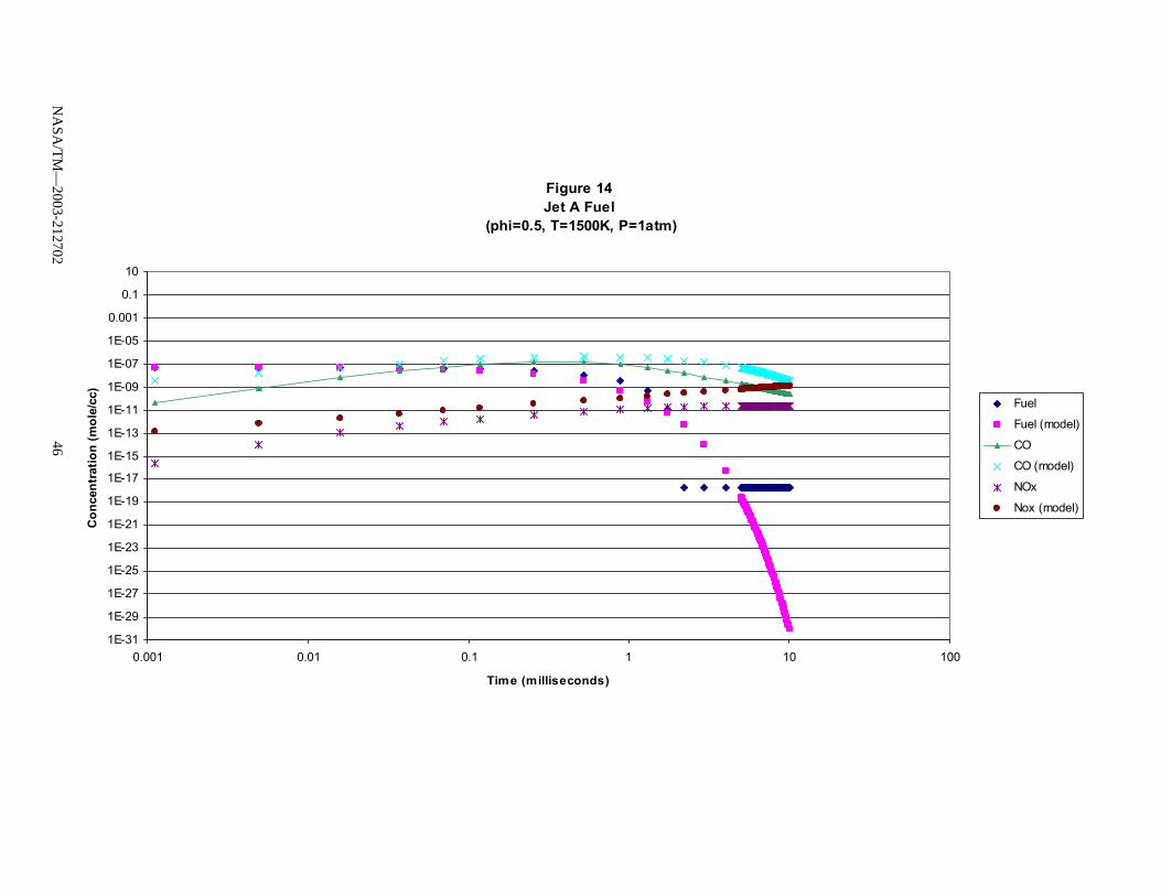
Figure 14Jet A Fuel
(phi=0.5, T=1500K, P=1atm)
1E-31
1E-29
1E-27
1E-25
1E-23
1E-21
1E-19
1E-17
1E-15
1E-13
1E-11
1E-09
1E-07
1E-05
0.001
0.1
10
0.001 0.01 0.1 1 10 100
Time (milliseconds)
Con
cent
ratio
n (m
ole/
cc)
Fuel
Fuel (model)
CO
CO (model)
NOx
Nox (model)
NA
SA/T
M—
2003-21270246
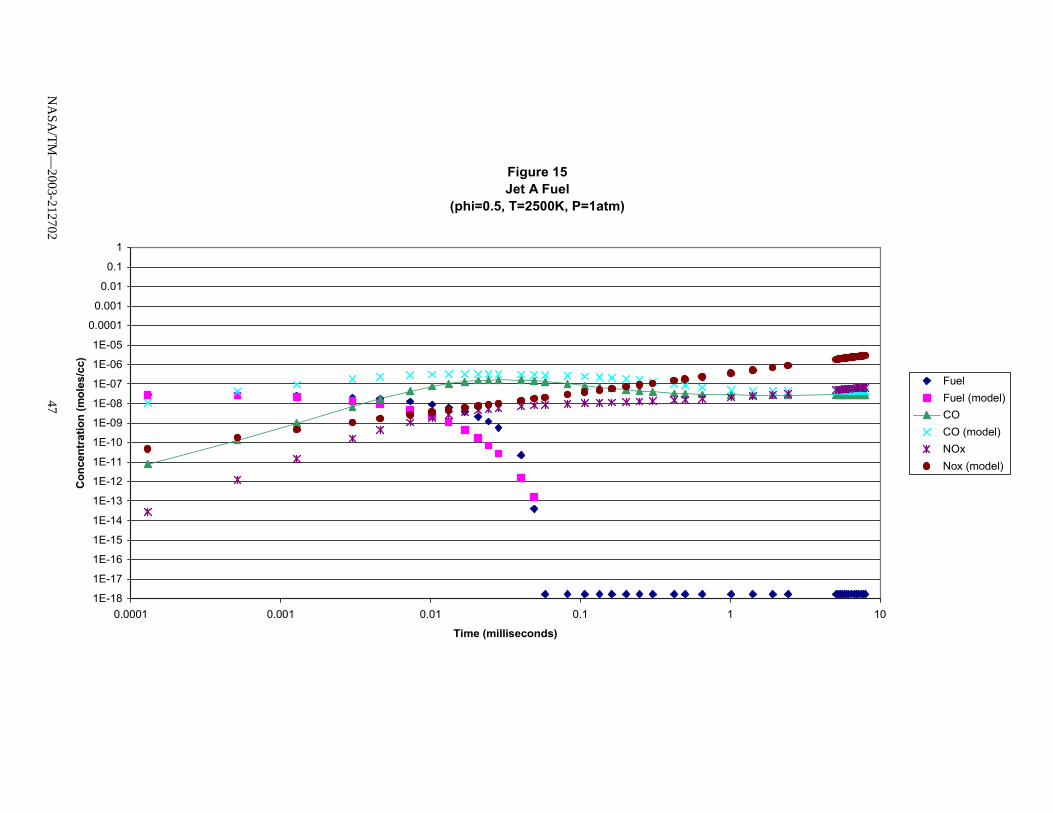
Figure 15Jet A Fuel
(phi=0.5, T=2500K, P=1atm)
1E-18
1E-17
1E-16
1E-15
1E-14
1E-13
1E-12
1E-11
1E-10
1E-09
1E-08
1E-07
1E-06
1E-05
0.0001
0.001
0.01
0.1
1
0.0001 0.001 0.01 0.1 1 10
Time (milliseconds)
Con
cent
ratio
n (m
oles
/cc)
Fuel Fuel (model)CO CO (model)NOxNox (model)
NA
SA/T
M—
2003-21270247
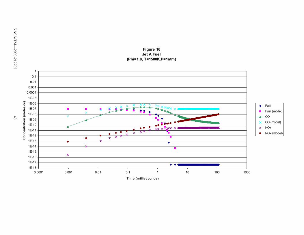
Figure 16Jet A Fuel
(Phi=1.0, T=1500K,P=1atm)
1E-18
1E-171E-16
1E-151E-14
1E-13
1E-121E-11
1E-101E-09
1E-08
1E-071E-06
1E-05
0.00010.001
0.010.1
1
0.0001 0.001 0.01 0.1 1 10 100 1000
Time (milliseconds)
Con
cent
ratio
n (m
oles
/cc)
Fuel
Fuel (model)
CO
CO (model)
NOx
NOx (model)
NA
SA/T
M—
2003-21270248
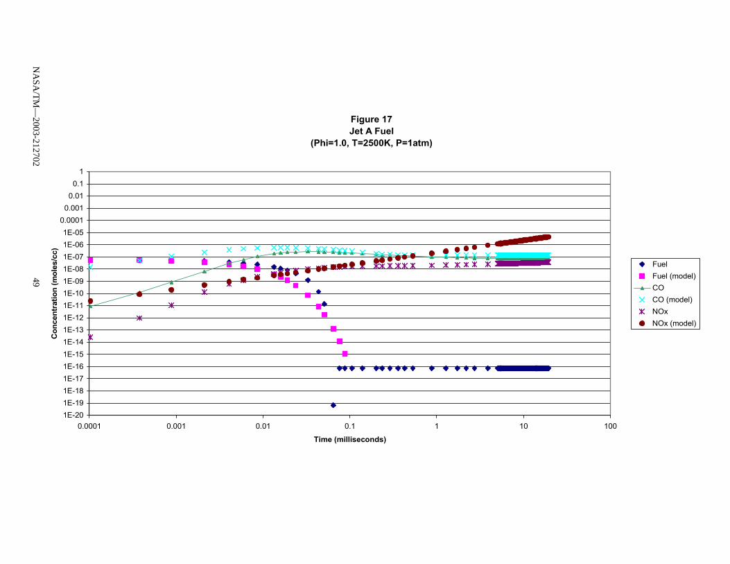
Figure 17Jet A Fuel
(Phi=1.0, T=2500K, P=1atm)
1E-201E-191E-181E-171E-161E-151E-141E-131E-121E-111E-101E-091E-081E-071E-061E-05
0.00010.0010.010.1
1
0.0001 0.001 0.01 0.1 1 10 100
Time (milliseconds)
Con
cent
ratio
n (m
oles
/cc)
Fuel Fuel (model)COCO (model)NOxNOx (model)
NA
SA/T
M—
2003-21270249
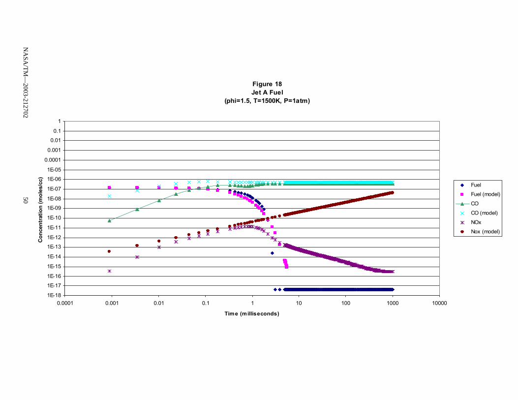
Figure 18Jet A Fuel
(phi=1.5, T=1500K, P=1atm)
1E-18
1E-17
1E-16
1E-15
1E-14
1E-13
1E-12
1E-11
1E-10
1E-09
1E-08
1E-07
1E-06
1E-05
0.0001
0.001
0.01
0.1
1
0.0001 0.001 0.01 0.1 1 10 100 1000 10000
Time (milliseconds)
Con
cent
ratio
n (m
oles
/cc)
Fuel
Fuel (model)
CO
CO (model)
NOx
Nox (model)
NA
SA/T
M—
2003-21270250
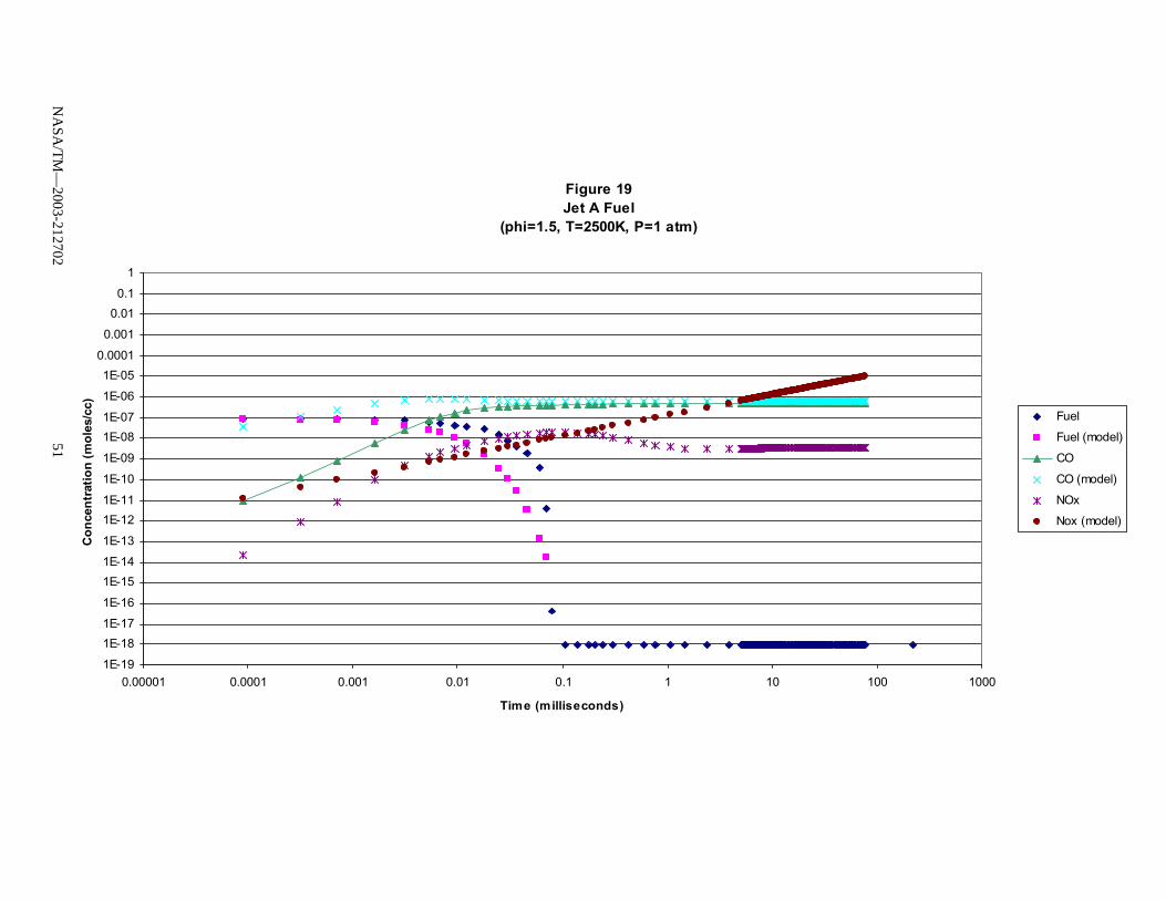
Figure 19Jet A Fuel
(phi=1.5, T=2500K, P=1 atm)
1E-19
1E-181E-17
1E-16
1E-151E-14
1E-13
1E-121E-11
1E-10
1E-09
1E-081E-07
1E-06
1E-050.0001
0.001
0.010.1
1
0.00001 0.0001 0.001 0.01 0.1 1 10 100 1000
Time (milliseconds)
Con
cent
ratio
n (m
oles
/cc)
Fuel
Fuel (model)
CO
CO (model)
NOx
Nox (model)
NA
SA/T
M—
2003-21270251
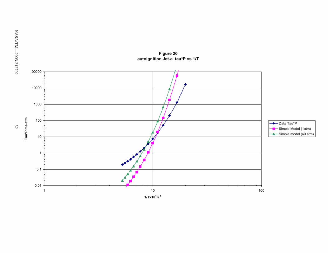
Figure 20autoignition Jet-a tau*P vs 1/T
0.01
0.1
1
10
100
1000
10000
100000
1 10 100
1/Tx104K-1
Tau*
P m
s-at
m
Data Tau*PSimple Model (1atm)Simple model (40 atm)
NA
SA/T
M—
2003-21270252
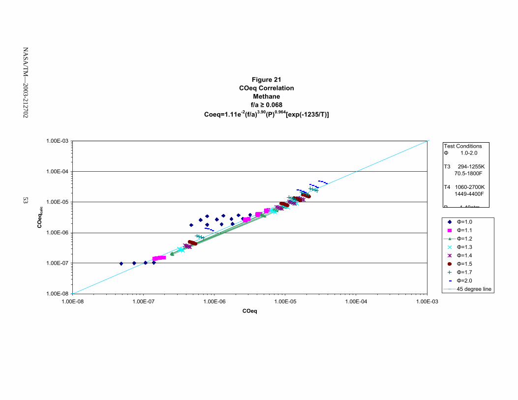
Figure 21COeq Correlation
Methanef/a ≥ 0.068
Coeq=1.11e-2(f/a)3.90(P)0.964[exp(-1235/T)]
1.00E-08
1.00E-07
1.00E-06
1.00E-05
1.00E-04
1.00E-03
1.00E-08 1.00E-07 1.00E-06 1.00E-05 1.00E-04 1.00E-03
COeq
CO
eqca
lc
Φ=1.0Φ=1.1Φ=1.2Φ=1.3Φ=1.4Φ=1.5Φ=1.7Φ=2.045 degree line
Test ConditionsΦ 1.0-2.0
T3 294-1255K 70.5-1800F
T4 1060-2700K 1449-4400F
P 1 40atm
NA
SA/T
M—
2003-21270253
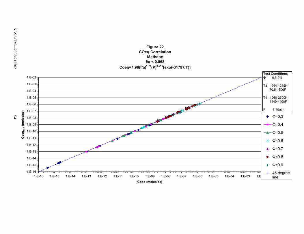
Figure 22COeq Correlation
Methanef/a < 0.068
Coeq=4.98(f/a)1.74(P)0.512[exp(-31797/T)]
1.E-16
1.E-15
1.E-14
1.E-13
1.E-12
1.E-11
1.E-10
1.E-09
1.E-08
1.E-07
1.E-06
1.E-05
1.E-04
1.E-03
1.E-02
1.E-16 1.E-15 1.E-14 1.E-13 1.E-12 1.E-11 1.E-10 1.E-09 1.E-08 1.E-07 1.E-06 1.E-05 1.E-04 1.E-03 1.E-02
Coeq (moles/cc)
Coe
q cal
c (m
oles
/cc)
Φ=0.3
Φ=0.4
Φ=0.5
Φ=0.6
Φ=0.7
Φ=0.8
Φ=0.9
45 degreeline
Test ConditionsΦ 0.3-0.9
T3 294-1255K 70.5-1800F
T4 1060-2700K 1449-4400F
P 1-40atm
NA
SA/T
M—
2003-21270254

Figure 23CH4 Fuel Tau Parity
(lean 7/31 cut off data)
1.00E-04
1.00E-03
1.00E-02
1.00E-01
1.00E+00
1.00E+01
1.00E+02
1.00E+03
1.00E+04
1.00E+05
1.00E-04 1.00E-03 1.00E-02 1.00E-01 1.00E+00 1.00E+01 1.00E+02 1.00E+03 1.00E+04 1.00E+05
tau (milliseconds)
tau
calc
(mill
isec
onds
)
NA
SA/T
M—
2003-21270255
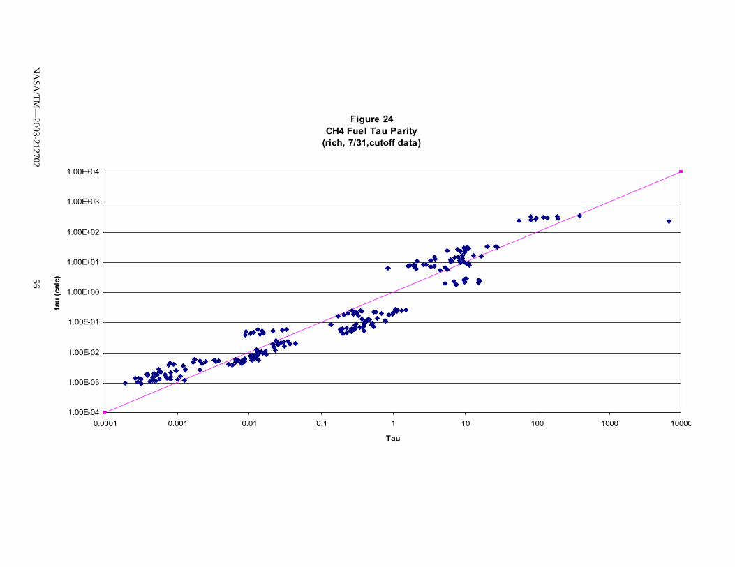
Figure 24CH4 Fuel Tau Parity
(rich, 7/31,cutoff data)
1.00E-04
1.00E-03
1.00E-02
1.00E-01
1.00E+00
1.00E+01
1.00E+02
1.00E+03
1.00E+04
0.0001 0.001 0.01 0.1 1 10 100 1000 10000
Tau
tau
(cal
c)
NA
SA/T
M—
2003-21270256
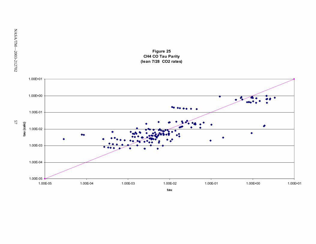
Figure 25CH4 CO Tau Parity
(lean 7/28 CO2 rates)
1.00E-05
1.00E-04
1.00E-03
1.00E-02
1.00E-01
1.00E+00
1.00E+01
1.00E-05 1.00E-04 1.00E-03 1.00E-02 1.00E-01 1.00E+00 1.00E+01
tau
tau
(cal
c)
NA
SA/T
M—
2003-21270257
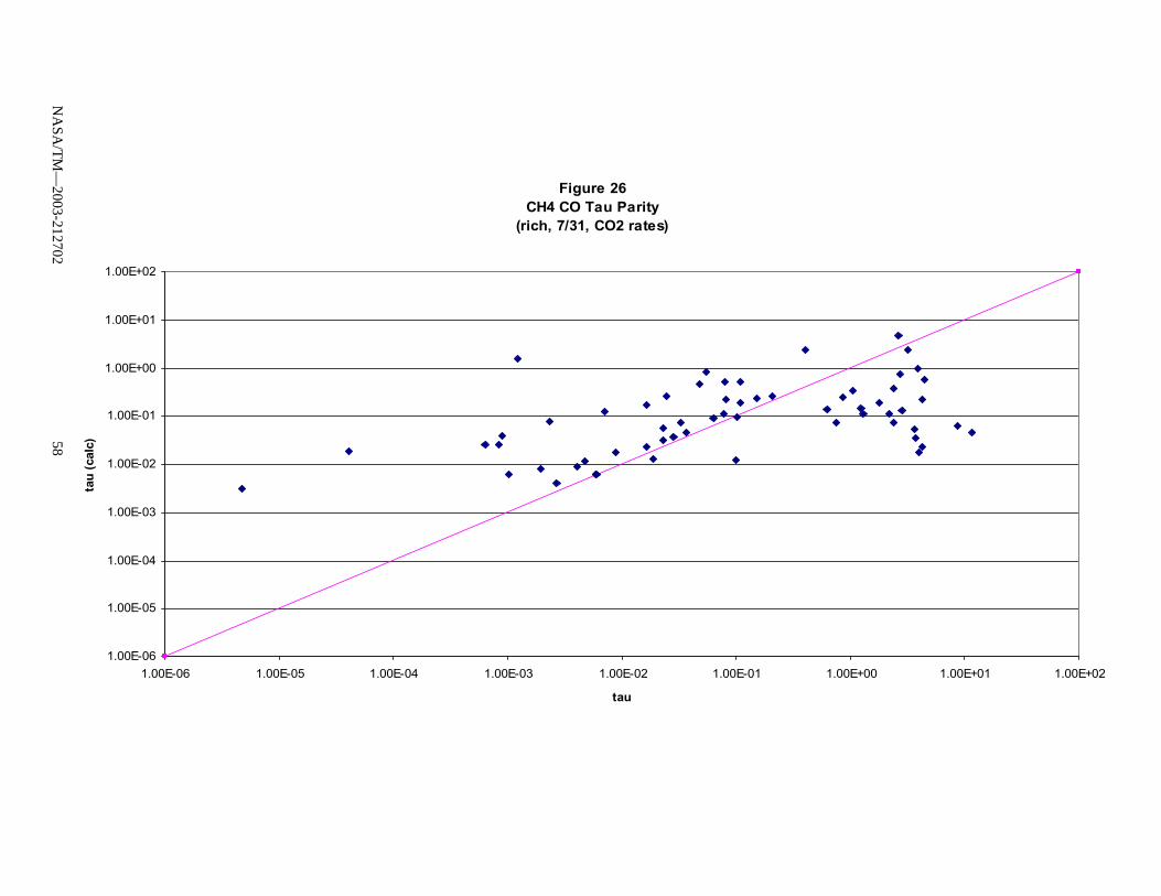
Figure 26CH4 CO Tau Parity
(rich, 7/31, CO2 rates)
1.00E-06
1.00E-05
1.00E-04
1.00E-03
1.00E-02
1.00E-01
1.00E+00
1.00E+01
1.00E+02
1.00E-06 1.00E-05 1.00E-04 1.00E-03 1.00E-02 1.00E-01 1.00E+00 1.00E+01 1.00E+02
tau
tau
(cal
c)
NA
SA/T
M—
2003-21270258
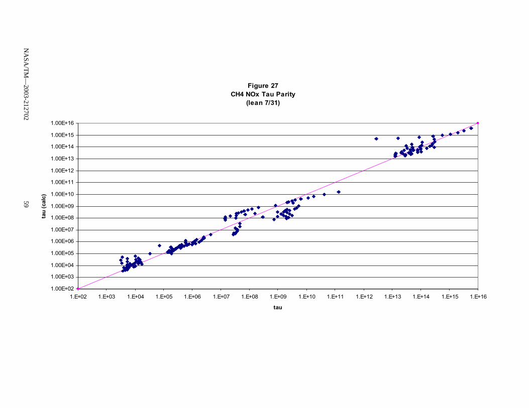
Figure 27CH4 NOx Tau Parity
(lean 7/31)
1.00E+02
1.00E+03
1.00E+04
1.00E+05
1.00E+06
1.00E+07
1.00E+08
1.00E+09
1.00E+10
1.00E+11
1.00E+12
1.00E+13
1.00E+14
1.00E+15
1.00E+16
1.E+02 1.E+03 1.E+04 1.E+05 1.E+06 1.E+07 1.E+08 1.E+09 1.E+10 1.E+11 1.E+12 1.E+13 1.E+14 1.E+15 1.E+16
tau
tau
(cal
c)
NA
SA/T
M—
2003-21270259
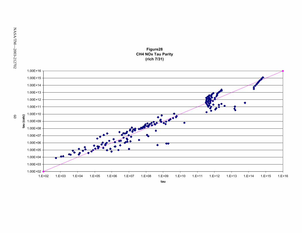
Figure28CH4 NOx Tau Parity
(rich 7/31)
1.00E+02
1.00E+03
1.00E+04
1.00E+05
1.00E+06
1.00E+07
1.00E+08
1.00E+09
1.00E+10
1.00E+11
1.00E+12
1.00E+13
1.00E+14
1.00E+15
1.00E+16
1.E+02 1.E+03 1.E+04 1.E+05 1.E+06 1.E+07 1.E+08 1.E+09 1.E+10 1.E+11 1.E+12 1.E+13 1.E+14 1.E+15 1.E+16
tau
tau
(cal
c)
NA
SA/T
M—
2003-21270260
This publication is available from the NASA Center for AeroSpace Information, 301–621–0390.
REPORT DOCUMENTATION PAGE
2. REPORT DATE
19. SECURITY CLASSIFICATION OF ABSTRACT
18. SECURITY CLASSIFICATION OF THIS PAGE
Public reporting burden for this collection of information is estimated to average 1 hour per response, including the time for reviewing instructions, searching existing data sources,gathering and maintaining the data needed, and completing and reviewing the collection of information. Send comments regarding this burden estimate or any other aspect of thiscollection of information, including suggestions for reducing this burden, to Washington Headquarters Services, Directorate for Information Operations and Reports, 1215 JeffersonDavis Highway, Suite 1204, Arlington, VA 22202-4302, and to the Office of Management and Budget, Paperwork Reduction Project (0704-0188), Washington, DC 20503.
NSN 7540-01-280-5500 Standard Form 298 (Rev. 2-89)Prescribed by ANSI Std. Z39-18298-102
Form Approved
OMB No. 0704-0188
12b. DISTRIBUTION CODE
8. PERFORMING ORGANIZATION REPORT NUMBER
5. FUNDING NUMBERS
3. REPORT TYPE AND DATES COVERED
4. TITLE AND SUBTITLE
6. AUTHOR(S)
7. PERFORMING ORGANIZATION NAME(S) AND ADDRESS(ES)
11. SUPPLEMENTARY NOTES
12a. DISTRIBUTION/AVAILABILITY STATEMENT
13. ABSTRACT (Maximum 200 words)
14. SUBJECT TERMS
17. SECURITY CLASSIFICATION OF REPORT
16. PRICE CODE
15. NUMBER OF PAGES
20. LIMITATION OF ABSTRACT
Unclassified Unclassified
Technical Memorandum
Unclassified
National Aeronautics and Space AdministrationJohn H. Glenn Research Center at Lewis FieldCleveland, Ohio 44135–3191
1. AGENCY USE ONLY (Leave blank)
10. SPONSORING/MONITORING AGENCY REPORT NUMBER
9. SPONSORING/MONITORING AGENCY NAME(S) AND ADDRESS(ES)
National Aeronautics and Space AdministrationWashington, DC 20546–0001
Available electronically at http://gltrs.grc.nasa.gov
November 2003
NASA TM—2003-212702
E–14205
WBS–22–708–87–16
60
Reduced Equations for Calculating the Combustion Rates of Jet-Aand Methane Fuel
Melissa Molnar and C. John Marek
Chemical kinetics; Methane; Jet-A; Time constants
Unclassified -UnlimitedSubject Categories: 07 and 28 Distribution: Nonstandard
Melissa Molnar, Ohio University, Department of Chemical Engineering, Athens, Ohio 45701 and Summer Intern atOhio Aerospace Institute; and C. John Marek, NASA Glenn Research Center. Responsible person, C. John Marek,organization code 5830, 216–433–3584.
Simplified kinetic schemes for Jet-A and methane fuels were developed to be used in numerical combustion codes, suchas the National Combustor Code (NCC) that is being developed at Glenn. These kinetic schemes presented here result in acorrelation that gives the chemical kinetic time as a function of initial overall cell fuel/air ratio, pressure, and temperature.The correlations would then be used with the turbulent mixing times to determine the limiting properties and progress ofthe reaction. A similar correlation was also developed using data from NASA’s Chemical Equilibrium Applications (CEA)code to determine the equilibrium concentration of carbon monoxide as a function of fuel air ratio, pressure, and tempera-ture. The NASA Glenn GLSENS kinetics code calculates the reaction rates and rate constants for each species in a kineticscheme for finite kinetic rates. These reaction rates and the values obtained from the equilibrium correlations were thenused to calculate the necessary chemical kinetic times. Chemical kinetic time equations for fuel, carbon monoxide, andNOx were obtained for both Jet-A fuel and methane.