Embed Size (px)
Citation preview

Reduced Complexity Signal Detectionand Channel Estimation for Iterative
MIMO-OFDM Systems
Licai Fang
This thesis is presented for the degree of Doctor of PhilosophySchool of Electrical, Electronic and Computer Engineering
May 2016

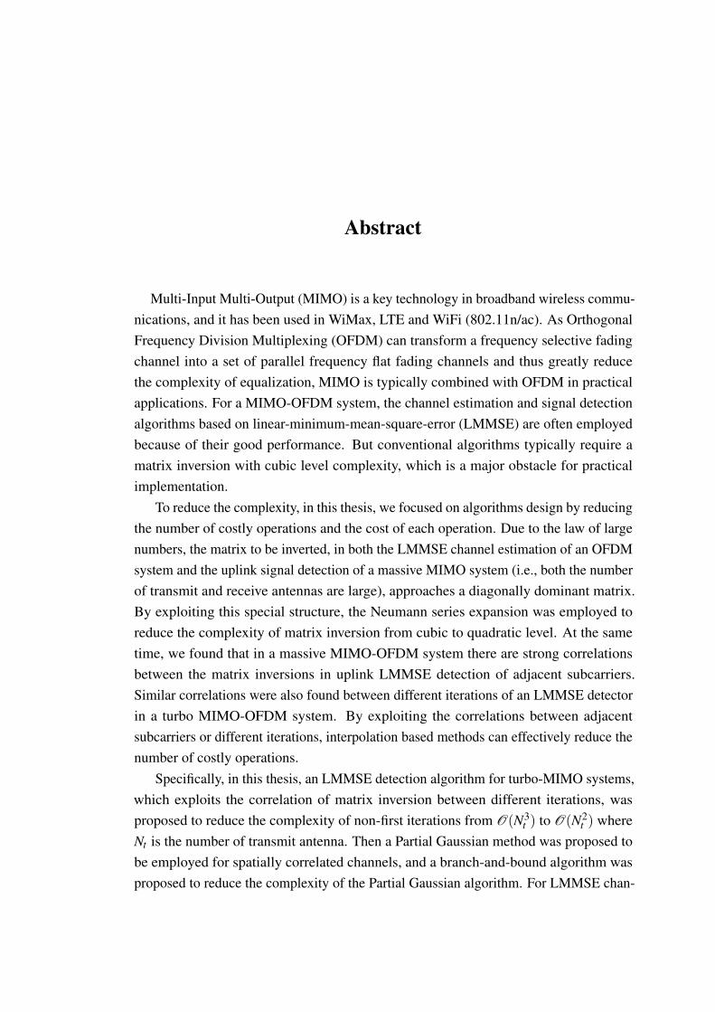
Abstract
Multi-Input Multi-Output (MIMO) is a key technology in broadband wireless commu-nications, and it has been used in WiMax, LTE and WiFi (802.11n/ac). As OrthogonalFrequency Division Multiplexing (OFDM) can transform a frequency selective fadingchannel into a set of parallel frequency flat fading channels and thus greatly reducethe complexity of equalization, MIMO is typically combined with OFDM in practicalapplications. For a MIMO-OFDM system, the channel estimation and signal detectionalgorithms based on linear-minimum-mean-square-error (LMMSE) are often employedbecause of their good performance. But conventional algorithms typically require amatrix inversion with cubic level complexity, which is a major obstacle for practicalimplementation.
To reduce the complexity, in this thesis, we focused on algorithms design by reducingthe number of costly operations and the cost of each operation. Due to the law of largenumbers, the matrix to be inverted, in both the LMMSE channel estimation of an OFDMsystem and the uplink signal detection of a massive MIMO system (i.e., both the numberof transmit and receive antennas are large), approaches a diagonally dominant matrix.By exploiting this special structure, the Neumann series expansion was employed toreduce the complexity of matrix inversion from cubic to quadratic level. At the sametime, we found that in a massive MIMO-OFDM system there are strong correlationsbetween the matrix inversions in uplink LMMSE detection of adjacent subcarriers.Similar correlations were also found between different iterations of an LMMSE detectorin a turbo MIMO-OFDM system. By exploiting the correlations between adjacentsubcarriers or different iterations, interpolation based methods can effectively reduce thenumber of costly operations.
Specifically, in this thesis, an LMMSE detection algorithm for turbo-MIMO systems,which exploits the correlation of matrix inversion between different iterations, wasproposed to reduce the complexity of non-first iterations from O(N3
t ) to O(N2t ) where
Nt is the number of transmit antenna. Then a Partial Gaussian method was proposed tobe employed for spatially correlated channels, and a branch-and-bound algorithm wasproposed to reduce the complexity of the Partial Gaussian algorithm. For LMMSE chan-

iv
nel estimation of OFDM systems, a low complexity algorithm based on Neumann seriesexpansion was investigated. This proposed algorithm can achieve mean-square error(MSE) performance close to the optimal LMMSE estimator but with only O(N logL)complexity where N is the number of subcarriers and L is the number of time domainchannel coefficients taps. With the aid of turbo processing, we also proposed a data-aidedchannel estimator which can track time-varying channels caused by terminals movement(up to 100 km/hour) with very low pilot overhead.
We also investigated medium-sized massive MIMO systems. A low cost LMMSEdetection algorithm based on Neumann series expansion for uplink applications wasproposed. Compared to alternative algorithms, the algorithm can significantly reducethe total detection complexity to O(KNtNr) where Nr is the number of receive antennaand K (typically K < 3) is the number of Neumann series expansion. The computationsaving comes from the fact that proposed algorithm can not only avoid computing matrixinversion but also replace matrix-matrix multiplications with matrix-vector multiplica-tions.

List of Publications
[1] L. Fang, and D. Huang. Neumann Series Expansion Based LMMSE ChannelEstimation for OFDM Systems. IEEE Communications Letters, vol. 20, no. 4, pp.748-751, April 2016. (Chapter 4)
[2] L. Fang, L. Xu, and D. Huang. Low complexity iterative MMSE-PIC detec-tion for medium-size massive MIMO. IEEE Wireless Communications Letters,5(1):108–111, Feb 2016. (Chapter 5)
[3] Licai Fang, Lu Xu, Qinghua Guo, Defeng Huang, and S. Nordholm. A lowcomplexity iterative soft-decision feedback MMSE-PIC detection algorithm formassive MIMO. In 2015 IEEE International Conference on Acoustics, Speech andSignal Processing (ICASSP), pages 2939–2943, 2015. (Chapter 2)
[4] Licai Fang, Lu Xu, Qinghua Guo, D.D. Huang, and S. Nordholm. A hybrid iterativeMIMO detection algorithm: Partial Gaussian approach with integer programming.In 2014 IEEE/CIC International Conference on Communications in China (ICCC),pages 463–468, 2014. (Chapter 3)


Acknowledgements
First, I would like to thank my supervisors Prof. David (Defeng) Huang andDr. Qinghua Guo for their support, for giving me the opportunity to pursue my Ph.D.Without their directions, enlightenments and encouragements, this thesis would havebeen impossible.
Then I would like to thank the colleagues in the Signal Processing Wireless Commu-nication Laboratory (SPWCL) research group at the University of Western Australia,namely, Dr. Lu Xu, Dr. Jindan Yang, Dr. Hang Li and Dr. T.-U. I. Khandoker. Theirinsightful academic discussion is invaluable to my research.
Most importantly, my sincere thanks go to my wife Dr. Wei Hou and our families.Their consistent supports are the main driving force for me to finish this thesis duringmy 40s.


Table of contents
List of Publications v
List of figures xiii
List of tables xv
1 Introduction 11.1 Background . . . . . . . . . . . . . . . . . . . . . . . . . . . . . . . . 1
1.1.1 MIMO . . . . . . . . . . . . . . . . . . . . . . . . . . . . . . 11.1.2 Turbo Principle . . . . . . . . . . . . . . . . . . . . . . . . . . 31.1.3 OFDM . . . . . . . . . . . . . . . . . . . . . . . . . . . . . . 4
1.2 Turbo MIMO-OFDM System . . . . . . . . . . . . . . . . . . . . . . . 51.2.1 Channel . . . . . . . . . . . . . . . . . . . . . . . . . . . . . . 61.2.2 LDPC Encoder and Decoder . . . . . . . . . . . . . . . . . . . 81.2.3 Soft Mapper and Soft Demapper . . . . . . . . . . . . . . . . . 111.2.4 Signal Detection . . . . . . . . . . . . . . . . . . . . . . . . . 151.2.5 Channel Estimation . . . . . . . . . . . . . . . . . . . . . . . . 19
1.3 Motivations and Contributions . . . . . . . . . . . . . . . . . . . . . . 221.3.1 Signal Detection . . . . . . . . . . . . . . . . . . . . . . . . . 221.3.2 Channel Estimation . . . . . . . . . . . . . . . . . . . . . . . . 24
1.4 Notations . . . . . . . . . . . . . . . . . . . . . . . . . . . . . . . . . 26
2 A Low Complexity Soft-Decision Feedback MMSE-PIC Detection Algo-rithm 272.1 System Model . . . . . . . . . . . . . . . . . . . . . . . . . . . . . . . 282.2 Gaussian Model Based MMSE Detection Algorithm . . . . . . . . . . 292.3 Complexity Reduction . . . . . . . . . . . . . . . . . . . . . . . . . . 30
2.3.1 Low Complexity Matrix Inversion . . . . . . . . . . . . . . . . 302.3.2 A Heuristic Approach to Solve the Stability Problem . . . . . . 32

x Table of contents
2.3.3 Computational Complexity Comparison . . . . . . . . . . . . . 32
2.3.4 Iterative Method to Improve First-pass Performance . . . . . . 33
2.4 Simulation Results . . . . . . . . . . . . . . . . . . . . . . . . . . . . 34
2.4.1 Simulation Setup . . . . . . . . . . . . . . . . . . . . . . . . . 34
2.4.2 BER Performance . . . . . . . . . . . . . . . . . . . . . . . . 35
2.5 Conclusion . . . . . . . . . . . . . . . . . . . . . . . . . . . . . . . . 36
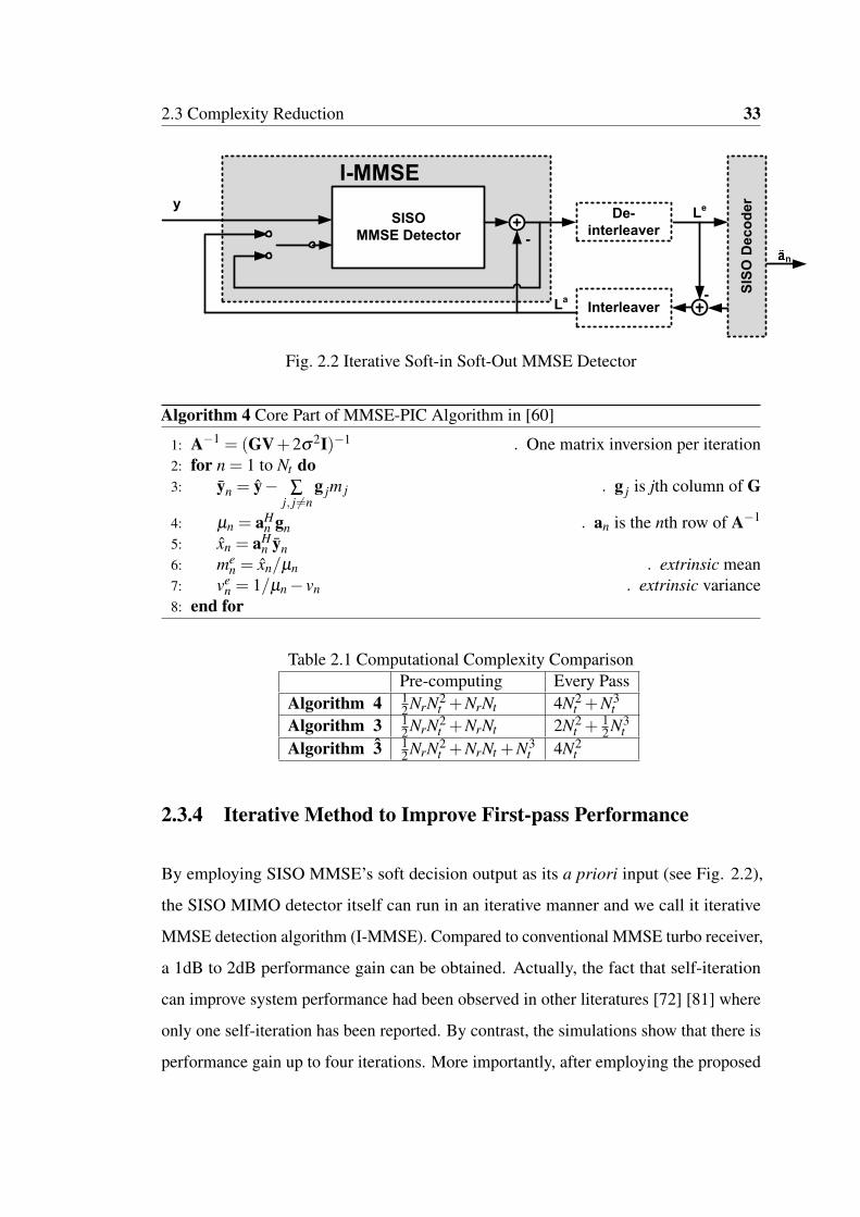
3 MIMO Detection Algorithm: Partial Gaussian Approach with Integer Pro-gramming 393.1 Introduction . . . . . . . . . . . . . . . . . . . . . . . . . . . . . . . . 39
3.2 System Model . . . . . . . . . . . . . . . . . . . . . . . . . . . . . . . 40
3.3 Partial Gaussian Approach with Integer Programming . . . . . . . . . . 42
3.3.1 PGA Detection Algorithm . . . . . . . . . . . . . . . . . . . . 42
3.3.2 Simplified Marginalization Calculation . . . . . . . . . . . . . 42
3.3.3 Resolving QIP with the Branch-and-Bound algorithm . . . . . . 45
3.4 Simulation Results . . . . . . . . . . . . . . . . . . . . . . . . . . . . 47
3.4.1 Simulation Setup . . . . . . . . . . . . . . . . . . . . . . . . . 47
3.4.2 BER Performance . . . . . . . . . . . . . . . . . . . . . . . . 48
3.4.3 Complexity . . . . . . . . . . . . . . . . . . . . . . . . . . . . 49
3.5 Conclusion . . . . . . . . . . . . . . . . . . . . . . . . . . . . . . . . 49
4 A Low Cost LMMSE Channel Estimator for OFDM Systems 514.1 Introduction . . . . . . . . . . . . . . . . . . . . . . . . . . . . . . . . 51
4.2 System Model . . . . . . . . . . . . . . . . . . . . . . . . . . . . . . . 52
4.3 LMMSE Channel Estimation . . . . . . . . . . . . . . . . . . . . . . . 53
4.4 Newmann Series Expansion Based Channel Estimation . . . . . . . . . 54
4.4.1 Neumann Series Expansion . . . . . . . . . . . . . . . . . . . 54
4.4.2 Computational Complexity Comparison . . . . . . . . . . . . . 56
4.5 Simulation Results . . . . . . . . . . . . . . . . . . . . . . . . . . . . 56
4.5.1 Mean-Square Error (MSE) Performance for Time-Invariant Chan-nels . . . . . . . . . . . . . . . . . . . . . . . . . . . . . . . . 57
4.5.2 Bit Error Rate (BER) Performance for Iterative Systems . . . . 58
4.6 Discussion . . . . . . . . . . . . . . . . . . . . . . . . . . . . . . . . . 60
4.6.1 The Power Delay Profile (PDP) . . . . . . . . . . . . . . . . . 60
4.6.2 The Assumption of Quasi-static Channel . . . . . . . . . . . . 60
4.7 Conclusion . . . . . . . . . . . . . . . . . . . . . . . . . . . . . . . . 61

Table of contents xi
5 Low Complexity Iterative MMSE-PIC Detection for Medium-Size MassiveMIMO 635.1 Introduction . . . . . . . . . . . . . . . . . . . . . . . . . . . . . . . . 635.2 System Model . . . . . . . . . . . . . . . . . . . . . . . . . . . . . . . 655.3 MMSE Detection Based on Neumann Series Expansion . . . . . . . . . 66
5.3.1 Neumann Series Expansion . . . . . . . . . . . . . . . . . . . 685.3.2 Computational Complexity Comparison . . . . . . . . . . . . . 685.3.3 Discussion . . . . . . . . . . . . . . . . . . . . . . . . . . . . 69
5.4 Simulation Results . . . . . . . . . . . . . . . . . . . . . . . . . . . . 695.5 Conclusion . . . . . . . . . . . . . . . . . . . . . . . . . . . . . . . . 71
6 A Novel Interpolation Algorithm for Massive MIMO OFDM System Detec-tion 736.1 Introduction . . . . . . . . . . . . . . . . . . . . . . . . . . . . . . . . 736.2 System Model and Soft-output MMSE Detector . . . . . . . . . . . . . 746.3 MMSE Detection Based on Interpolation . . . . . . . . . . . . . . . . . 76
6.3.1 Correlation of Matrix Inversion for Massive MIMO-OFDMSystems . . . . . . . . . . . . . . . . . . . . . . . . . . . . . . 76
6.3.2 Interpolation Based Matrix Inversion . . . . . . . . . . . . . . 796.3.3 Computational Complexity Comparison . . . . . . . . . . . . . 80
6.4 BER Performance . . . . . . . . . . . . . . . . . . . . . . . . . . . . . 826.5 Conclusion . . . . . . . . . . . . . . . . . . . . . . . . . . . . . . . . 82
7 Summary and Future Work 857.1 Summary . . . . . . . . . . . . . . . . . . . . . . . . . . . . . . . . . 857.2 Future Work . . . . . . . . . . . . . . . . . . . . . . . . . . . . . . . . 86
7.2.1 Channel estimation for MIMO-OFDM systems . . . . . . . . . 867.2.2 Channel estimation for Massive MIMO . . . . . . . . . . . . . 867.2.3 Uplink Signal Detection for Massive MIMO-OFDM . . . . . . 87
Appendix A Proof of the Equality of Algorithm 1 and Algorithm 2 89
Bibliography 93


List of figures
1.1 An Iterative MIMO-OFDM Communication System . . . . . . . . . . 51.2 QC-LDPC Base Parity Check Matrix . . . . . . . . . . . . . . . . . . . 81.3 4-PAM Constellation Diagram . . . . . . . . . . . . . . . . . . . . . . 14
2.1 Iterative Detection and Decoding of a MIMO Communication System . 292.2 Iterative Soft-in Soft-Out MMSE Detector . . . . . . . . . . . . . . . . 332.3 BER Performance Comparison Between Exact Implementation and
Proposed Approximation for a 16×16 MIMO System. . . . . . . . . . 342.4 BER Performance Comparison Between Different Number of Self-
iterations for 32×32 MIMO. . . . . . . . . . . . . . . . . . . . . . . . 352.5 BER Performance Comparison Between Different Number of Self-
iterations for 16×16 MIMO. . . . . . . . . . . . . . . . . . . . . . . . 372.6 BER Performance Comparison Between Different Number of Self-
iterations for 4×4 MIMO. . . . . . . . . . . . . . . . . . . . . . . . . 38
3.1 Iterative Detection and Decoding of a MIMO Communication System . 403.2 An example of the proposed branch and bound algorithm where d is the
tree level, lb means low bound, ub means upper bound and m∗ is thevector that minimizes f (m). Because the first heuristic solution happensto be the final solution, there are only 6 nodes visited. . . . . . . . . . . 46
3.3 BER performances of 16-QAM 40×40 MIMO with correlation factorρ = 0.5 and ρ = 0.8. . . . . . . . . . . . . . . . . . . . . . . . . . . . 48
3.4 BER performance comparison between PGA-Exact and PGA-IP under16-QAM 40×40 MIMO correlated channel (ρ = 0.4) . . . . . . . . . . 50
4.1 MSE performance with different L at SNR of 14dB . . . . . . . . . . . 554.2 MSE performance for the 10-tap COST259_RAx channel . . . . . . . . 574.3 BER performance for 10-tap COST259_RAx Channel at speed of 100
km/hour . . . . . . . . . . . . . . . . . . . . . . . . . . . . . . . . . . 59

xiv List of figures
4.4 MSE Under Channel No.1-6 . . . . . . . . . . . . . . . . . . . . . . . 62
5.1 BER performance comparison for exact MMSE, proposed and SORbased [1] with MIMO size of K ×M = 16×128 . . . . . . . . . . . . . 70
6.1 Correlations of Ch(d) and Cg(d) of adjacent subcarriers with N = 64,Nt = 20, different ρ and different subcarrier distance d. . . . . . . . . . 77
6.2 Correlations of Ch(d) and Cg(d) of adjacent subcarriers (with differentd) under different channel models with N = 64, Nt = 20 and ρ = 8. . . 79
6.3 Complexity comparison with ρ = 8, N = 128 and I = 5 . . . . . . . . . 816.4 BER performance comparison for exact MMSE, Matched filter, Pro-
posed Vpn with exact Hn and Proposed Vp
n with interpolated Hn forNt ×Nr = 16×128 MIMO. . . . . . . . . . . . . . . . . . . . . . . . . 83

List of tables
2.1 Computational Complexity Comparison . . . . . . . . . . . . . . . . . 33
3.1 Average CPU run time (s) comparison between MMSE_PIC, PGA_IPand PGA_Exact for detecting 2000bits with 3 iterations under 40×40MIMO with 16-QAM on a X86 Linux PC . . . . . . . . . . . . . . . . 49
4.1 Simulated Channel Models [2] . . . . . . . . . . . . . . . . . . . . . . 61
5.1 Computational Complexity Comparison . . . . . . . . . . . . . . . . . 69
6.1 Simulated Channel Models [2] . . . . . . . . . . . . . . . . . . . . . . 786.2 Computational Complexity Comparison . . . . . . . . . . . . . . . . . 80


Chapter 1
Introduction
1.1 Background
1.1.1 MIMO
In late 1980’s, the multiple-input multiple-output antenna (MIMO) systems was pro-
posed for wireless communications. By using multiple antennas at both transmitter
and receiver side, MIMO can create multiple parallel channels using the same radio
spectrum [3] [4]. MIMO techniques can improve communications performance by either
increasing reliability or maximizing throughput. In order to increase reliability, some
form of space-time coding (STC) is typically employed to combat multipath scatting
by creating spatial diversity [5]. While for improving throughput, spatial multiplexing
techniques [6] [7] are employed to exploit multipath scatting. It was shown that the
achievable transmitting rate of MIMO systems scales as min(Nt ,Nr)log(1+SNR) and
the link outage scales as SNRNtNr [8] where Nt and Nr are the numbers of transmitter
and receiver antennas, respectively.
MU-MIMO
For the cellular systems, the conventional MIMO technology has some limitations
because the terminals can not employ many antennas due to the cost, power and size

2 Introduction
constraint. Another issue of conventional MIMO is the propagation limitations; in case
of LOS (line-of-sight) propagation, channel rank loss or antenna correlation, the spatial
multiplexing gain in conventional MIMO will be severely degraded [9]. To achieve the
gain of multiple access capacity and overcome above two issues, the multi-user MIMO
(MU-MIMO) scheme had been proposed and researched in recent years. By treating
every user’s terminal as a virtual MIMO antenna, the MIMO spatial multiplexing gain
can be preserved. Although the individual users will not experience increased throughput
by MU-MIMO, but the overall system performance will improve dramatically. So many
state-of-the-art wireless communication standards have adopted MU-MIMO, like 3GPP
long-term evolution advanced (3GPP LTE-A)(Release 10) [10], IEEE 802.16m (WiMAX
Profile 2.0) [11] and Wifi (802.11ac) [12].
Massive MIMO
With the maturing of MU-MIMO, by making the number of antennas much larger at Base
Station side, comes the concept of massive MIMO, which is characterized with hundreds
of antennas at Base Station and can serve tens of terminals simultaneously. Massive
MIMO can reap all the benefits of conventional MIMO and MU-MIMO in a much
greater scale [13] [14]. Firstly, high energy efficiency can be obtained by focusing the
energy with extreme sharpness into small regions in space. Specifically, by appropriately
shaping the signals sent out by the antennas, all radio wave fronts collectively emitted by
all antennas interfere constructively at the intended terminals, but destructively almost
everywhere else. [15] illustrated that the energy focus effect by comparing M = 10
transmit antennas (M-element Uniform Linear Array (ULA)) and M = 100 antennas. It
shows that when the number of transmit antenna at the transmitter is 100, by applying
spatial precoding, the field strength can be focused to a point rather than in a certain
direction as done in conventional MIMO or MU-MIMO. This energy focus property can
greatly reduce the interference between spatially separated users and reduce the total
radiated signal power, thereby the Base Station can benefit from this property to greatly
reduce the total output RF power. At the same time, based on information theory [15],

1.1 Background 3
massive MIMO can increase the spectral efficiency 10+ times from the aggressive spatial
multiplexing.
Besides the above base station scenario where the communication is multipoint-
to-point for uplink or point-to-multipoint for downlink, there is also point-to-point
applications like the back-haul connections between base stations. For this kind of
configuration, a large number of antennas can be used both at transmit and receive base
stations.
It is also worth noting that when the number of receive antennas at the base station is
large and much larger than the total number of transmit antennas in user terminals, a
simple detection algorithm such as a matched filter can achieve very good performance,
as with the assumption of i.i.d. entries for channel matrix H, the channel vectors become
orthogonal to each other and HHH converges to a scaled identity matrix. But from
practical implementation point of view, medium size antenna arrays are also of interest.
1.1.2 Turbo Principle
Nearly at the same time as the emerging of MIMO technology, the invention of turbo
codes and iterative decoding [16] paved the way for achieving system performance
close to the Shannon limit. By exchanging information between several decoding
units iteratively, the system performance was shown to be close to optimal decoding,
but with feasible complexity. Then the “turbo principle” [16] was used to improve
performance of other tasks in the wireless receiver, e.g., equalization [17] [18] [19],
channel estimation [20], multi-user detection [21] and MIMO detection [22] [23] [24].
For a coded communication system, as the complexity of the optimal receiver is
exponential in the length of the data transmitted, most practical receivers include two
separate blocks: signal detection and channel decoding. The signal detectors have been
designed to process the received observations to account for the effects of the channel
and to estimate the transmitted channel symbols that best fit the observed data. Then the
soft information (in the form of Log-Likelihood Ratio (LLR)) is passed to the channel
decoder for decoding.

4 Introduction
Applying the “turbo principle” to this kind of receiver, comes the iterative detection
and decoding (IDD) system. In IDD, a soft-input and soft-out detector is required which
can accept soft information from the decoder and output soft information to the decoder.
In general, only extrinsic information can be exchanged between the detector and the
decoder [25].
“Turbo principle” can also be applied to the task of channel estimation. In order to
track channel variation caused by movement of terminals, data-aided scheme is often
employed. For slow fading channel with preamble-type pilots, the channel coefficients
copied from last symbol can be improved by exploiting the soft or hard information
feedback from the decoder as the virtual pilot [26]. Similarly, for superimposed-type
pilot, it is common to perform iterative channel estimation and decoding by exploiting
data fed back from the channel decoder [20].
1.1.3 OFDM
Most modern wireless communication systems are broadband systems which have high
data rates. As a result, the symbol rate is much higher than the channel coherence
bandwidth and thus the channel is frequency selective. The major issue about frequency
selective fading is the inter-symbol interference (ISI), which is caused by the fact that the
symbol period is shorter than the delay spread. To combat with ISI, one way is to employ
equalization with single carrier. As the computational complexity of equalization is
quite high, another popular technique for coping with frequency-selective fading effects
is using orthogonal frequency division multiplexing (OFDM).
The idea behind OFDM is to split a broadband signal that experiences frequency-
selective fading into multiple narrow sub-bands (subcarrier) so that each subcarrier
experiences flat fading. Because the bandwidths of the sub-bands is less than the
coherence bandwidth of the channel, each sub-stream is far less vulnerable to the ISI
than the original input stream. At the same time, although each OFDM subcarrier
is narrowband , the bandwidth of the OFDM symbol is greater than the coherence
bandwidth of a frequency selective channel. To mitigate the effects of the ISI between
1.2 Turbo MIMO-OFDM System 5
OFDM symbols, guard intervals are inserted between OFDM symbols so that time
dispersion of current OFDM symbol will not interfere with subsequent OFDM symbols.
In practice, an OFDM symbol is obtained by taking the inverse discrete Fourier trans-
form (IDFT) of a block of modulation symbols at the transmitter. Then at the receiver
the forward discrete Fourier transform (DFT) is performed to restore the modulated
symbols. As both the IDFT and DFT can be implemented using fast Fourier transform
(FFT) algorithms, OFDM is considered as a low cost technique.
1.2 Turbo MIMO-OFDM System
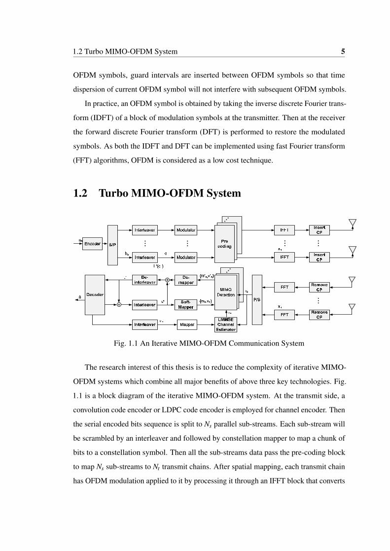
Fig. 1.1 An Iterative MIMO-OFDM Communication System
The research interest of this thesis is to reduce the complexity of iterative MIMO-
OFDM systems which combine all major benefits of above three key technologies. Fig.
1.1 is a block diagram of the iterative MIMO-OFDM system. At the transmit side, a
convolution code encoder or LDPC code encoder is employed for channel encoder. Then
the serial encoded bits sequence is split to Ns parallel sub-streams. Each sub-stream will
be scrambled by an interleaver and followed by constellation mapper to map a chunk of
bits to a constellation symbol. Then all the sub-streams data pass the pre-coding block
to map Ns sub-streams to Nt transmit chains. After spatial mapping, each transmit chain
has OFDM modulation applied to it by processing it through an IFFT block that converts

6 Introduction
a block of modulated constellation points to a time domain block of symbols followed
by adding the cyclic prefix (CP). The resulting baseband sequence of symbols in each
chain are then passed to the analog and RF blocks before being applied to a transmit
antenna.
At the receive side, after the CP of the data received on every receive antenna is
removed, FFT will be performed to generate the frequency domain symbols. Then
the channel estimator estimates the frequency domain channel coefficients based on
the received pilot data. With the frequency domain channel coefficients, the MIMO
detection is performed on every subcarrier. The detected data is then de-mapped to
soft information (typically in LLR format) and sent to the channel decoder. In an IDD
system, the decoded bits (or soft information) will be sent back (after re-mapping them
to symbols) to the channel estimator and/or the symbol detector to purify the results of
last iteration.
1.2.1 Channel
The nature of the wireless environment results in the transmitted signal experiencing var-
ious forms of corruption including noise and fading. The background noise and thermal
noise of the channel are the major contributors of noise which is commonly modelled
as additive white Gaussian noise (AWGN). Fading, which is the variation of the signal
amplitude over time and frequency, may either be due to multipath propagation, referred
to as multi-path fading, or to shadowing from obstacles that affect the propagation of a
radio wave, referred to as shadow fading.
The fading phenomenon can be broadly classified into two different types: large-
scale fading and small-scale fading. The large-scale fading is characterized by average
path loss and shadowing. On the other hand, small-scale fading refers to the result of
multipath propagation. In a wireless environment, the transmitted signal may be scattered
into multiple paths as a result of reflection and refraction off environmental obstacles and
atmospheric effects. An attenuated version of the transmitted signal propagates through
each path and arrives at the receiver at different times. Consequently, the received signal

1.2 Turbo MIMO-OFDM System 7
is distorted by one symbol interfering with subsequent symbols, which is commonly
referred as inter symbol interference (ISI).
Characteristics of a multipath fading channel are often specified by a power delay
profile (PDP). Using a PDP, different signal paths are characterized by their relative delay
(τi) and average power (P(τi)). Then the RMS delay spread στ can be calculated by the
square root of the second central moment of PDP as στ =√
τ2 − τ2 where the mean
excess delay τ is given by the first moment of PDP as τ = ∑k τkP(τk)∑k P(τk)
and τ2 =∑k τ2
k P(τk)
∑k P(τk).
In general, the coherence bandwidth, denoted as Bc, is inversely-proportional to the
RMS delay spread, that is, Bc ≈ 1στ
.
Fading Due to Time Dispersion
Due to time dispersion, a transmit signal may undergo fading over a frequency domain
either in a selective or non-selective manner, which is referred to as frequency-selective
fading and frequency-flat fading. For the given channel frequency response, frequency
selectivity is generally governed by signal bandwidth. When the signal bandwidth (Bs ∝
1/Ts, Ts is the symbol period) is narrow compared with the coherence bandwidth (Bc)
of the channel, the signal experiences flat fading; otherwise, it experiences frequency-
selective fading.
Fading Due to Frequency Dispersion
Variation in the time domain is closely related to movement of the transmitter or receiver,
which incurs a spread in the frequency domain, known as a Doppler shift. The maximum
Doppler shift can be calculated by fm = vmax fC/c0 where vmax is the maximum velocity
between the receiver antenna and the transmitter antenna, fC is the frequency of carrier
and c0 is the speed of electromagnetic wave. Depending on the extent of the Doppler
spread, the received signal undergoes fast or slow fading. When the coherence time
Tc ≈ 1fm
is smaller than the symbol period Ts (Ts > Tc), a channel impulse response
quickly varies within the symbol period. Under this condition, the transmit signal is
subject to fast fading.

8 Introduction
1.2.2 LDPC Encoder and Decoder
Low-density parity-check (LDPC) codes are linear block codes which can provide near-
capacity performance. They were proposed by Gallager in his dissertation [27] in 1960.
Then in 1981 Tanner generalized LDPC codes and introduced a graphical representation
of LDPC codes in [28]. In mid-1990’s Mackay, Luby and others [29] [30] [31] also
independently discovered the advantages of spare parity-check matrices. The most
obvious character of LDPC codes is that the parity-check matrix has a low density of 1’s
for binary LDPC codes. For a LDPC code with (n− k)×n parity-check matrix H, if the
number of 1’s in each column wc equals to the number of 1’s in each row wr, this code
is called regular LDPC code and otherwise called irregular LDPC code with the code
rate of k/n.
A special subclass of LDPC codes, called Quasi-Cyclic LDPC (QC-LDPC) codes
has received much attention because of their superb error correction performance [27].
QC-LDPC codes is characterized that a cyclic shift of one codeword results in another
codeword and due to this regular structure their encoding is proved to be linear with
code length. As QC-LDPC has near capacity performance and can be decoded by
low-complexity iterative decoding algorithm, it has been adopted by many industrial
standards like IEEE 802.11n, IEEE 802.11ac and IEEE 802.16e, as an error correction
code [32] [12] [33].
LDPC Encoder Algorithm
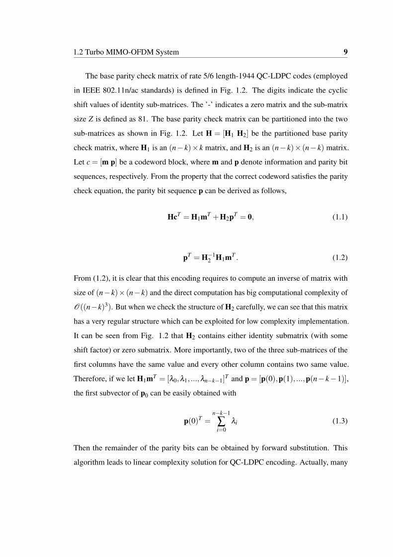
Fig. 1.2 QC-LDPC Base Parity Check Matrix
1.2 Turbo MIMO-OFDM System 9
The base parity check matrix of rate 5/6 length-1944 QC-LDPC codes (employed
in IEEE 802.11n/ac standards) is defined in Fig. 1.2. The digits indicate the cyclic
shift values of identity sub-matrices. The ’-’ indicates a zero matrix and the sub-matrix
size Z is defined as 81. The base parity check matrix can be partitioned into the two
sub-matrices as shown in Fig. 1.2. Let H = [H1 H2] be the partitioned base parity
check matrix, where H1 is an (n− k)× k matrix, and H2 is an (n− k)× (n− k) matrix.
Let c = [m p] be a codeword block, where m and p denote information and parity bit
sequences, respectively. From the property that the correct codeword satisfies the parity
check equation, the parity bit sequence p can be derived as follows,
HcT = H1mT +H2pT = 0, (1.1)
pT = H−12 H1mT . (1.2)
From (1.2), it is clear that this encoding requires to compute an inverse of matrix with
size of (n−k)× (n−k) and the direct computation has big computational complexity of
O((n−k)3). But when we check the structure of H2 carefully, we can see that this matrix
has a very regular structure which can be exploited for low complexity implementation.
It can be seen from Fig. 1.2 that H2 contains either identity submatrix (with some
shift factor) or zero submatrix. More importantly, two of the three sub-matrices of the
first columns have the same value and every other column contains two same value.
Therefore, if we let H1mT = [λ0,λ1, ...,λn−k−1]T and p = [p(0),p(1), ...,p(n− k−1)],
the first subvector of p0 can be easily obtained with
p(0)T =n−k−1
∑i=0
λi (1.3)
Then the remainder of the parity bits can be obtained by forward substitution. This
algorithm leads to linear complexity solution for QC-LDPC encoding. Actually, many

10 Introduction
efforts now focus on how to improve encoding throughput and reduce implementation
complexity at the same time [34] [35].
LDPC Decoder Algorithm
Based on the Tanner graph representation of LDPC codes, the iterative massage passing
algorithm (MPA) is typically exploited to do the decoding. Tanner graph is a kind
of bipartite graph whose nodes can be separated into two types, and edges may only
connect two nodes of different types. These two nodes in Tanner graph are the variable
nodes (v-node) and the check nodes (c-node). The Tanner graph is drawn based on
the following rule: check node j is connected to variable node i whenever element h ji
of parity check matrix H is a 1. So, it is easy to know that there are m = n− k check
nodes for check equations and n variable nodes for code bits. The task of LDPC decoder
is to compute the a posteriori probability (APP) for a bit in the transmit codeword
c = [c0,c1, ...,cn−1] equals 1 given the received word y = [y0,y1, ...,yn] in LLR:
L(ci) = log(
Pr(ci = 0|y)Pr(ci = 1|y)
). (1.4)
When drawing a Tanner graph, typically we put the c-nodes above the v-nodes. Then
the message passing from a v-node i to a c-node j is noted as m↑i j. This extrinsic
information message is the probability of Pr(ci = b | input message), b ∈ {0,1} which
comes from channel input and all its neighbours excluding the c-node itself. In the
reverse direction, the message passing from a c-node to a v-node m↓ ji is the probability
of Pr(check equation f j is satisfied | input message). Now we introduce the following
notations [36]:
• Vj=v-nodes connected to c-node f j
• Ci=c-nodes connected to v-node ci
• Mv(i) = messages from all v-nodes except node ci
• Mc( j) = messages from all c-nodes except node f j
1.2 Turbo MIMO-OFDM System 11
• Pi = Pr(ci = 1 | yi)
• Si = event that the check equations involving ci are satisfied
• qi j(b) = Pr(ci = b | Si,yi,Mc( j)
), where b ∈ {0,1}. For LLR format, m↑i j =
log[qi j(0)]/qi j(1)]
• r ji(b) = Pr(check equation f j is satisfied | ci = b,Mv(i)
), where b ∈ {0,1}. For
LLR format, m↓ ji = log[r ji(0)/r ji(1)
]Then, the MPA can be summarized as follows,
• Step 1: Initialization: For every v-node, initialize pi = Pr(ci = 1|yi), then qi j(0) =
1− pi and qi j(1) = pi for each hi j = 1. Under AWGN channel, pi = 1/(1+
exp(2yi/σ2)).
• Step 2: For each c-node, update r ji by r ji(0) = 12 +
12 ∏
i′∈V j\i(1− 2qi′ j(1)) and
r ji(1) = 1− r ji(0).
• Step 3: Update qi j by qi j(0)=Ki j(1−Pi) ∏j′∈Ci\ j
r j′i(0), qi j(1)=Ki jPi ∏j′∈Ci\ j
r j′i(1)
and Ki j is selected to ensure that qi j(1)+qi j(0) = 1.
• Step 4: Update Qi by Qi(0) = Ki(1−Pi) ∏j∈Ci
r ji(0) and Qi(1) = KiPi ∏j∈Ci
r ji(1)
and Ki j is selected to ensure that Qi(1)+Qi(0) = 1.
• Step 5: Hard decision: For i = 0,1, ...,n− 1, if Qi(1) > Qi(0) then ci = 1; else
ci = 0.
• Step 6: If cHT = 0 or reaching the maximum iteration number, stop; else, go to
Step 2.
1.2.3 Soft Mapper and Soft Demapper
Soft Mapper
The function of a soft mapper module is to calculate the symbol mean and variance
from the extrinsic LLRs of code bits coming from the Soft-Input Soft-Output (SISO)

12 Introduction
decoder [37]. The soft mapper calculates {mn,vn} based on extrinsic LLR L(cn) using
the following equations:
mn = E(xn) =2Q
∑i=1
αi p(xn = αi) (1.5)
vn =Cov(xn,xn) =2Q
∑i=1
|αi|2 p(xn = αi)−m2n (1.6)
where each constellation symbol αi corresponds to a binary vector si = [si,1,si,2, ...,si,Q]T ,
and the symbol’s probability p(xn = αi) can be calculated as:
p(xn = αi) =Q
∏j=1
p(cn, j = si, j) (1.7)
while p(cn, j = si, j) is the probability of a code bit, which is normally represented by
LLR:
L j = lnp(cn, j = 0)p(cn, j = 1)
= lnp(cn, j = 0)
1− p(cn, j = 0). (1.8)
With (1.5) - (1.7), the computational complexity is O(Q2Q). When high order mod-
ulation is exploited, the computational complexity is high and the low complexity
algorithms can be found in [38] and [39].
Soft Demapper
In a coded system, the soft output from the equalizer (or detector) typically can greatly
improve the system BER performance compared to hard output. The symbol output
from equalizer (or detector) should be demapped to bit information in LLR format
which is the input requirement from most of the channel decoders like the Turbo code
or the LDPC code. When the soft output symbols are assumed as Gaussian distributed,
they can be described by their mean vector m and auto-covariance diagonal matrix V.
The task of the demapper is to compute the LLR for each code bit cn,q, which can be
1.2 Turbo MIMO-OFDM System 13
expressed as [18]
L(cn,q) = lnP(cn,q = 0|y)P(cn,q = 1|y)
= ln
∑xn∈A 0
q
P(xn|y)
∑xn∈A 1
q
P(xn|y)(1.9)
where A 0q (A 1
q ) denotes the subset of all αi ∈A corresponding to a binary subsequence
with the qth bit given by 0 (1). When IDD is adopted, only extrinsic information will be
passed to the channel decoder. The extrinsic LLR [17]
Le(cn,q) = L(cn,q)−La(cn,q)
= ln
∑xn∈A 0
q
P(y|xn)P(xn)
∑xn∈A 1
q
P(y|xn)P(xn)−La(cn,q)
(1.10)
will be the input to the decoder, where La(cn,q) is the output extrinsic LLR of the decoder
in the last iteration and P(xn) can be calculated from La(cn,q). The probability of the data
symbol xn being the constellation point αi is given by P(xn = αi) ∝ exp(− |αi−me
n|2ve
n
).
After some manipulation, we can get
Le(cn,q) = ln
∑αi∈A 0
q
exp(− |αi−me
n|2ve
n
)∏
q′ =qP(cn,q′ = si,q′)
∑αi∈A 1
q
exp(− |αi−me
n|2ve
n
)∏
q′ =qP(cn,q′ = si,q′)
(1.11)
Directly computing LLR in (1.11) needs exhaustively search every constellation point
which results high computational complexity if high order constellation is employed.
To reduce this complexity, quite a lot of works can be referred although they are
implemented in different background [38] [40]. The basic idea of these methods are
using the regularity of constellation points and employing the approximation used by
max_log_map algorithm in [41] to change the exhaustively search to a piecewise linear
combination. If we ignore the a priori information which has been found with little

14 Introduction
performance penalty and apply this approximation, (1.11) can be represented as
Le(cn,q)≈ ln
∑αi∈A 0
q
exp(− |αi−me
n|2ve
n
)∑
αi∈A 1q
exp(− |αi−me
n|2ve
n
)≈ 1
ven
maxαi∈A 0
q
(−|αi −men|2)−
1ve
nmax
αi∈A 1q
(−|αi −men|2)
=1ve
n
[min
αi∈A 1q
(|αi −men|2)− min
αi∈A 0q
(|αi −men|2)
](1.12)
Fig. 1.3 is a 4-PAM constellation diagram and the men is located in the × point. It is
0010 0111
5
3
5
15
1�
5
3✁
Fig. 1.3 4-PAM Constellation Diagram
easy to see that the results of the two min operation in (1.12) are the white constellation
point and the black one, and thus (1.12) can be easily calculated as follows:
Le(cn,0) =
1√5ve
n(4me
n −8) (men ≥ 0)
1√5ve
n(−4me
n −8) (men < 0)
(1.13)
and
Le(cn,1) =
1√5ve
n(8me
n −8) (men ≥ 2)
1√5ve
n(4me
n) (|men|< 2)
1√5ve
n(8me
n +8) (men ≤−2).
(1.14)

1.2 Turbo MIMO-OFDM System 15
1.2.4 Signal Detection
After the data symbols are transmitted over a MIMO channel and corrupted by AWGN,
the receiver receives superimposed and noised version of these symbols. The data
detection block is responsible for recovering those corrupted data symbols based on
certain estimation criterion. At the receiver side, in order to improve performance,
iterative detection and decoding can be employed based on the “turbo principle”. From
the iterative receiver diagram Fig. 1.1, it can be seen that the SISO decoder and the SISO
detector iteratively exchange soft extrinsic information between them.
The following is a brief review of conventional detection methods. If there is no
a-priori information available, the ML (Maximum Likelihood) method can be employed
while the MAP (Maximum a-Posteriori ) method can be employed if the a-priori in-
formation is available. But, both ML and MAP based methods suffer from the huge
computational complexity which is exponential in the number of transmit antenna Nt
and modulation constellation size Q. In order to reduce complexity, linear methods such
as zero forcing (ZF) or Minimum Mean Square Error (MMSE) can be employed. In
the family of non-linear detection algorithms, Sphere Decoding (SD) based search algo-
rithms have been deeply studied [42] [43]. Basically, SD algorithms have exponential
average complexity [3], and most importantly the complexity depends on channel status
and received SNR. In order to make the complexity deterministic, Fixed-Complexity
Sphere Decoder (FCSD) has been proposed with medium complexity and near ML per-
formance [43] [44]. Another non-linear detection is called Partial Gaussian method [45].
This algorithm has low and fixed computational complexity and near MAP performance
by using an adjustable parameter M. The basic idea behind this method is taking M
important symbols as discrete symbols but others as continuous. The continuous symbols
can be assumed to be Gaussian distributed which makes the whole computational com-
plexity very low. The last type of detection algorithm is based on factor graph [46] [47]
[17] [48] [49] [50] [51] [52].
In this thesis, we will focus on MIMO spatial multiplexing technique which can
transmit data at a higher speed than the system employing spatial diversity. Consider

16 Introduction
a MIMO-OFDM system with spatial multiplexing technique in Fig. 1.1 which has Nt
antennas at the transmit side, Nr antennas at the receiver side and N subcarriers. The
cyclic prefixes (CP) are inserted before the IFFT of x(n) to ensure the orthogonality
among the subcarriers and prevent inter-symbol interference (ISI) between consecutive
OFDM symbols. Considering a quasi-static channel which is constant during one OFDM
symbol, this OFDM system can be described as a set of parallel frequency flat additive
white Gaussian noise (AWGN) channels. Then the channel H can be denoted by a matrix
sized Nr ×Nt with its (i, j)th entry hi j denoting the channel gain between the ith transmit
antenna and the jth receive antenna where j ∈ [1,2, ...,Nr] and i ∈ [1,2, ...,Nt ]. So, for
every subcarrier, a length-Nr observation vector y at the receive side can be written as
y = Hx+w (1.15)
where w denotes a length-Nr circularly symmetric additive white Gaussian noise (AWGN)
vector with zero-mean and covariance of σ2I. It is worth noting that there are totally N
such equations in a MIMO-OFDM system.
Conventional Detection Algorithms
Linear signal detection algorithms like ZF and MMSE treat all other transmitted signals
as interferences and minimize or nullify these interferences when detecting the desired
signals. Specifically, according to the system model of (1.15), the ZF detection algorithm
can be described as:
xZF = (HHH)−1HHy (1.16)
while MMSE algorithm can be listed as
xMMSE = (HHH+σ2I)−1HHy (1.17)
where x is the detected transmit symbols. The noise enhancement effect of the above
two algorithms is significant when the condition number of the channel matrix is large

1.2 Turbo MIMO-OFDM System 17
(the minimum singular value is very small) [53] while the effect of noise enhancement
in MMSE algorithm is less critical than that in ZF algorithm.
In order to improve performance, Maximum likelihood (ML) is often employed
which calculates the Euclidean distance between the received signal vector and the
product of all possible transmitted signal vectors with the given channel H and finds the
one with the minimum distance. Mathematically, the ML algorithm can be described as:
xML = arg minx∈A Nt
(||y−Hx||2). (1.18)
It is obvious that the complexity of ML algorithm is exponential in Nt which is too
complex for a practical implementation, but its performance is much better than afore-
mentioned ZF and MMSE algorithms, especially for small-size MIMO. But for large
MIMO system, linear detection algorithms such as MMSE-PIC can have near optimal
performance [54]. To reduce the computational complexity of ML algorithm, search
based algorithms like Sphere Decoding (SD) can be exploited. After applying QL
decomposition to H (H = QL, QT Q = I and L is lower triangular), the problem (1.18)
can be visualized as a decision tree with Nt layers [55] as follows:
min{x1,x2,...,xNt }
f1(x1)+ f2(x1,x2)+ ...+ fNt (x1,x2, ...,xNt ) (1.19)
where fk(x1,x2, ...,xk) = (yk − ∑kl=1 Lk,lxl)
2 and y = Qy. The basic idea under SD
algorithm is to use efficient tree traversal algorithms to eliminate the number of nodes
visited and thus reduce the total complexity.
Soft-In Soft-Out Detection Algorithms for Turbo MIMO-OFDM Systems
The more reliable feedback from the decoder is a good information source to perform
interference cancellation. A lot of multi-user detection algorithms can be applied to
MIMO detection like the minimum mean square error parallel interference cancellation
(MMSE-PIC) algorithms [56] [57]. These algorithm involves a matrix inversion when
detecting every symbol. To reduce the complexity, an iterative method to implement

18 Introduction
the MMSE filter was proposed in [58]. Then [59] presented a method which needs pre-
computing one matrix inversion only and then detects every symbol with low complexity
incremental calculations. In 2011, [60] proposed a well optimized version of MMSE-PIC
with only one matrix inversion for detecting a block of data and implemented it in ASIC
which has been widely cited as the state-of-the-art MIMO detection implementation
benchmark. This algorithm is listed in Algorithm 1:
Algorithm 1 MMSE-PIC MIMO Detection Algorithm
Input: y,H, La
Output: Le ◃ extrinsic LLR value for every bit1: Compute the Gram matrix G = HHH and the matched filter output yMF = HHy.2: Compute the a priori soft-symbols m and variances V with (1.5) and (1.6).3: Perform PIC based on yMF according to yMF
i = HH yi = yMF −∑ j, j =i g jm j, j =1, ...,Nt where g j denotes the jth column of G.
4: Compute the matrix inversion of A−1 = (GV+σ2INt )−1.
5: Compute the MMSE filter outputs as µi = aHi gi and xi = aH
i yi, i = 1, ...,Nt , whereaH
i is the ith row of A−1.6: Compute the extrinsic variance and extrinsic mean by7: ve
i = 1/µi −18: me
n = xi/µi9: Compute LLRs Le(ci,q) with (1.12), i = 1, ...,Nt , q = 1, ...,Q.
Also in 2011, [17] proposed a generic method to implement a Soft-Input Soft-Output
(SISO) detector, where the a posteriori distribution of a multivariate Gaussian vector
was calculated first, followed by the calculation of the extrinsic information of each
individual variable. The calculation of multiple variables together naturally enables
sharing of computational units, thereby reducing system complexity. This algorithm is
described in Algorithm 2;
After applying this algorithm to MIMO detection, we found that although [17]
and [60] have very different formulae, they actually can generate the same extrinsic
mean and variance and thus the same soft-output to the channel decoder. The proof is
given in Appendix A.

1.2 Turbo MIMO-OFDM System 19
Algorithm 2 Gaussian model based MMSE detectionInput: y,H, La
Output: Le ◃ extrinsic LLR value for every bit1: Compute the Gram matrix G = HHH.2: Compute the a priori soft-symbols m and variances V with (1.5) and (1.6).3: Calculate the a posteriori mean mp and variance Vp by4: Vp = (V−1 + 1
2σ2 G)−1
5: mp = m+ 12σ2 Vp(HHy−Gm).
6: Calculate the extrinsic mean men and variance ve
n by7: ve
n = ( 1vp
n− 1
vn)−1
8: men = ve
n(mp
nvp
n− mn
vn).
9: Compute the LLRs Le(ci,q) with (1.12), i = 1, ...,Nt , q = 1, ...,Q.
1.2.5 Channel Estimation
In OFDM systems, a long enough cyclic prefixes (CP) insertion before the IFFT can
ensure the orthogonality among the subcarriers and prevent inter-symbol interference
(ISI) between consecutive OFDM symbols. Considering a quasi-static channel which
is constant during one OFDM symbol, this OFDM channel can be described as a set
of parallel additive white Gaussian noise (AWGN) channels. The orthogonality allows
each subcarrier component of the received signal to be expressed as the product of the
transmitted signal and channel frequency response at the subcarrier. Then the channel
can be estimated by using a preamble or pilot symbols known to both transmitter and
receiver for pilot subcarriers, then various interpolation techniques can be applied to
estimate the channel response of the subcarriers between pilot subcarriers. Depending on
the arrangement of pilots, four different types of pilot structures are typically employed.
• 1: Block Type: OFDM pilot symbols at all subcarriers are transmitted periodically.
Typically, a time domain interpolation is performed to get the whole channel
information. It is suitable for frequency-selective slow fading channels .
• 2: Comb Type: Every OFDM symbol has pilot tones at the periodically-located
subcarriers. It is suitable for fast-fading channels.

20 Introduction
• 3: Lattice Type: As a combination of block type and comb type, pilot tones are
inserted along both the time and frequency axes with given periods.
• 4: Superimposed Pilot: Low power of training (pilots) signal is added to the data
signal at the transmitter. The data-aided scheme, where the signal from the detector
or the channel decoder, is typically exploited to do interference cancellation for
the channel estimation.
Channel Estimation for OFDM System
After dropping the CP and performing FFT, the received frequency domain signal for
OFDM symbol n is given by
y(n) = X(n)η(n)+w(n) (1.20)
where y(n) denotes a length-N observation vector, X(n) ≡ diag{x(n)} denotes an
N × N diagonal matrix with x(n) (data transmitted in nth OFDM symbol, x(n) =
[x1,x2, · · · ,xN ]T ) on its diagonal, η(n) is the frequency domain channel coefficients and
w(n) denotes a length-N circularly symmetric AWGN vector with PDF C N (w;0,σ2I).
For notation simplicity, from now on we omit the time index n.
Pilot based channel estimation When training symbols are available the least-
square (LS ) and minimum-mean-square-error (MMSE) techniques are widely used for
channel estimation.
• HLS = X−1y, LS channel estimation.
• HMMSE = NFPFHXH(NXFPFHXH + σ2I)−1y, MMSE channel estimation,
where P is the channel power profile, F is the DFT matrix with the (k, l)th element
given by (F)k,l =√
Ne− j 2πklN with j =
√−1.
Although LS channel estimation has very low complexity, it suffers from noise
enhancement issue. In order to improve the performance of OFDM channel estimation,

1.2 Turbo MIMO-OFDM System 21
the DFT based channel estimation algorithm can be employed. Specifically, after taking
IDFT of the estimated frequency domain channel coefficients, we get the time domain
channel coefficients with length N. But the actual time domain coefficients only have
the length of L and typically L < N. By assigning the coefficients to zero for those with
index larger than L and transforming them back to frequency domain, we get the channel
estimation with better performance.
The MMSE channel estimation algorithm is much robust from noise enhancement but
the matrix inversion requires O(N3) complexity. To reduce the cubic complexity, there
are many algorithms have been proposed such as [61] [62] and [63] using windowed
discrete Fourier transform (WDFT) methods and [64] using Dual-Diagonal LMMS
algorithm.
Channel Estimation for MIMO-OFDM System
Classical channel estimation techniques for OFDM cannot be used in MIMO-OFDM
system directly, since the received signal is a superposition of signals transmitted from
different antennas for each OFDM subcarrier. The Expectation-Maximization (EM)
algorithm can convert a multiple-input channel estimation problem into a number of
single-input channel estimation problems [65].
MIMO-OFDM System Model In Fig. 1.1, the received signal on the mRth receive
antenna at time n after performing a DFT can be expressed as:
y(n)mR = X(n)FhmR(n)+w (1.21)
where y(n)mR = [ymR,1,ymR,2, ...,ymR,N ], X = [X1,X2, ...,XNT ] are the transmitted sym-
bols, XmT includes the symbols transmitted over N subcarriers from the mT th trans-
mit antenna on its diagonal, F = INT
⊗F and F is the truncated DFT matrix, with
[F]u,s = 1√N
e− j2πus/N , and u = 0, ...,N −1,s = 0, ...,L−1, hmR= [hT
1,mR, ...,hT
NT ,mR]T is
the time domain channel vector, with hmT ,mR= [hmT ,mR,0, ...,hmT ,mR,l, ...,hmT ,mR,L−1].

22 Introduction
LS for MIMO-OFDM The LS channel estimate for (1.21) is expressed as
hmR(n) = (FHXH(n)X(n)F)−1FHXH(n)y(n)mR (1.22)
Obviously, the matrix to be inverted is with the size of NT L×NT L and involves the
complexity of O(N3T L3).
1.3 Motivations and Contributions
1.3.1 Signal Detection
In massive MIMO applications [54], as the number of transmit antennas Nt is very large,
many of the conventional MIMO detection algorithms like Sphere Decoding (SD) [42]
have prohibitive complexity. As a result, new algorithms were proposed to reduce the
complexity [66]-[67]. In [66] and [68], two local neighborhood search methods known
as likelihood ascent search (LAS) and reactive tabu search (RTS) were presented. Both
can achieve near-optimal performance for BPSK or QPSK modulations but perform
poorly with high-order quadrature amplitude modulation (QAM). To further improve the
performance for high-order QAM, layered tabu search (LTS) was presented in [67] but
with much higher complexity. Interestingly, when turbo-processing is employed, recent
research shows that for massive MIMO and under well conditioned channels, the linear
detection method such as iterative minimum mean-squared error with soft interference
cancellation can achieve near optimal performance [54]. Together with the iterative
detection and decoding (IDD) technology, linear detection algorithm like the minimum
mean square error parallel interference cancellation (MMSE-PIC) algorithm [56] [57] is
attractive because of its low complexity and good bit error rate (BER) performance. To
reduce the burden of performing matrix inversion for detecting every symbol in MMSE-
PIC algorithm, some reduced complexity algorithms have been proposed [58] [59] and
implemented in ASIC [60] [69] which require only one matrix inversion to detect one
block of receive data.

1.3 Motivations and Contributions 23
For iterative MIMO detection application, the matrix inversion has to be computed
for every iteration because the a priori variance is different for every iteration. As
this matrix inversion varies only according to this a priori variance between different
iterations, it is possible that the second and the subsequent iterations can exploit the
matrix inversion result of the first pass thereby reducing the total complexity. Chapter 2
will focus on this topic.
With more and more antennas are employed in modern communication systems, the
physical limitation forces the system designer to reduce the space between different
antennas and thus leads to correlated channels. The spatial correlation between antennas
should be taken into account when performing signal detection. We found that for a turbo
massive MIMO system, the MMSE-PIC performs poorly under correlated channels and
the Partial Gaussian Algorithm (PGA) in [45] can handle correlation channel effectively.
But due to the marginalization of M discrete symbols in PGA is exponential in MQ (Q
is the number of bits in a symbol), it is obvious that with larger M (say M ≥ 3) PGA
algorithm will have high computational complexity. So in Chapter 3, we proposed an
approximation method and a search algorithm to reduce this complexity. Extensive
simulation shows that the approximation only causes marginal performance loss and the
proposed branch-and-bound algorithm has roughly 5% of the exact PGA algorithm’s
complexity.
Although the matched filter algorithm is optimal and with low complexity when
a large number of antennas are employed by the base station, for practical medium-
size massive MIMO, more complex algorithms have to be used for good performance.
Together with the IDD technology, MMSE-PIC algorithm [60] is attractive for detection
of medium-size massive MIMO signals. But the algorithm proposed in [60] still needs
cubic level complexity when detecting a block of data. To reduce this complexity,
[70] and [71] employ Neumann series expansion to avoid matrix inversion involved in
MMSE filter calculation. Then in [72] the authors proposed to use similar method to
perform 3GPP-LTE uplink signal detection and proved the convergence of the Neumann
series expansion.These works can all successfully avoid computing matrix inversion

24 Introduction
directly, and reduce complexity from O(N3t ) to O(N2
t ) where Nt is the total number of
antennas of end terminals. But they all need the pre-computed Gram matrix as an input.
The Gram matrix computation involves complexity of N2t Nr/2 which is much higher
than the matrix inversion of N3t /2 in massive MIMO uplink detection where Nr ≫ Nt
and Nr is the number of antennas in base station. This means that they cannot reduce the
total detection complexity significantly. This motives us to study the method that how
to reduce the total complexity. In Chapter 5, we proposed a novel detection algorithm
which can avoid both matrix inversion and matrix-matrix multiplication. The proposed
algorithm has the complexity of O(KNtNr) where K is the terms number of Neumann
series expansion (typically k ≤ 5).
Then we consider a medium-size massive MIMO-OFDM system. As the matched
filter detection algorithm cannot achieve good enough bit error rate (BER) performance,
the MMSE-PIC based Soft-Input Soft-Output (SISO) detector is often used for signal
detection of every data subcarrier. But because the number of tones N is typically large
and the MMSE-PIC algorithm involves cubic level complexity from a matrix inversion
and Gram calculation, the tone by tone (per subcarrier) detection methods still incur very
high computational complexity. Although there are works which can perform matrix
inversion using interpolation method, they were all designed for small-size MIMO and
cannot be easily extended to massive MIMO applications. In Chapter 6, we will exploit
the strong correlation between the MMSE matrix inversions of adjacent subcarriers and
propose a linear interpolation method to compute the matrix inversions thus significantly
reducing the number of matrix inversion required. Extensive simulations show that
the proposed algorithm can reduce the complexity to the matched filter level but with
significantly better BER performance than it.
1.3.2 Channel Estimation
Accurate channel estimation is an essential requirement for high performance signal
detection at the receiver. In an OFDM system, the frequency selective channel is of-
ten assumed time invariant within one OFDM symbol and the frequency correlation

1.3 Motivations and Contributions 25
among different subcarriers is often exploited to reduce the computational complexity
of the channel estimator. If the channel power delay profile (PDP) is available, the
linear-minimum-mean-square-error (LMMSE) estimation is typically employed with
the aid of pilot signals (and/or data fed back from the detector or the channel decoder).
However, directly implementing such an estimator typically involves a matrix inversion
with cubic complexity of channel length. To reduce the cubic complexity, windowed
discrete Fourier transform (WDFT) methods were proposed in [61] [62] [63] to achieve
a complexity of O(N logN) (N is the number of subcarriers) but with significant per-
formance loss. In [73], using the law of large numbers, an approximation to the matrix
inversion was proposed to reduce the complexity to O(N logN). However, this incurs a
mean-square error (MSE) floor in the high signal-to-noise ratio (SNR) region. In [64], a
Dual-Diagonal LMMSE channel estimation for OFDM systems was proposed and the
corresponding MSE was analyzed. With this method, the channel estimation can be
achieved with complexity of O(N logN) and the MSE performance is close to the exact
LMMSE algorithm from low to medium SNR. But for high SNR, both the simulation
results and MSE analysis showed that there is still some performance loss. Recently,
basis expansion model (BEM) algorithms based on discrete prolate spheroidal (DPS)
sequences have attracted much interest as they need no channel statistics but the knowl-
edge of the maximum delay spread and the maximum Doppler spread. Assuming that the
CIR is invariant within one OFDM symbol, a low complexity Linear MMSE estimation
of time-frequency variant channels for MIMO-OFDM systems was proposed in [74]
by replacing a two-dimensional Slepian-basis expansion with two serially concatenated
one-dimensional Slepian-basis expansions. Then in [75], the time variant CIR within
one OFDM symbol was taken into account and algorithms with complexity of O(N2)
were proposed. These DPS based algorithms were well designed for fast-fading environ-
ment. For block fading channels, [76] proposed several DPS based algorithms with low
complexity.
In this thesis, by employing the fact that the matrix to be inverted in MMSE channel
estimation is diagonally dominant1, we proposed to use a K terms Neumann series
26 Introduction
expansion in Chapter 4 to approximate the inversion. In this way, the matrix inversion
can be implemented with Fast Fourier Transform (FFT) or Inverse Fast Fourier Transform
(IFFT) operations with L inputs or L outputs, thus has the complexity of O(N logL)
where L is the number of time domain channel taps. It is worth noting that the proposed
channel estimation algorithm has close MSE performance as the exact implementation
from low to high SNR. In this chapter, we also found that with the knowledge of the
number of channel taps (i.e. L) and SNR, an uniform distributed PDP can be used to
replace the exact PDP with marginal performance loss, which is desirable because the
exact PDP is typically difficult to obtain.
1.4 Notations
The notations used in this thesis are as follows. Lower and upper case letters denote
scalars. Bold lower and upper case letters represent column vectors and matrices,
respectively. As customary, given a matrix Q we will let Qi j denote its entry in ith row
and jth column, and vi is used to present the ith element of a vector v. We use ∝ to
denote equality of functions up to a scale factor. The superscriptions “T ” and “H” denote
the transpose and conjugate transpose, respectively. Let IN denote an N ×N identity
matrix, E[·] the expectation operation and tr{·} the trace operation. The function of
diag{a} returns a diagonal matrix with vector a being the main diagonal and {M}diag
returns M with the off-diagonal elements of M set to be zero. The probability density
function (PDF) of a continuous random variable and the probability mass function of a
discrete random variable are represented by p(·) and P(·), respectively.
1A square matrix A is called diagonally dominant if |Aii| ≥ ∑ j =i |Ai j| for all i, where Ai j denotes theentry in the ith row and jth column.

Chapter 2
A Low Complexity Soft-Decision
Feedback MMSE-PIC Detection
Algorithm
In [17], a generic method to implement a Soft-Input Soft-Output (SISO) detector was
proposed, where the a posteriori distribution of a multivariate Gaussian vector was
calculated first, followed by the calculation of the extrinsic information of each individual
variable. The calculation of multiple variables together naturally enables sharing of
computational units, thereby reducing system complexity. So in this chapter, we firstly
employ [17] to implement the MMSE-PIC in MIMO applications, which can reduce
system complexity as the matrix to be inverted is a Hermitian positive definite (HPD)
matrix with size Nt ×Nt (Nr and Nt are the number of receive antennas and transmit
antennas, respectively). A HPD matrix enables us to use the more computational efficient
matrix inversion method.
In order to reduce the complexity of the second and subsequent iterations, we derive
a new method to calculate the matrix inversion by a linear combination of two matrices
which have been computed in the first pass (from the detector to the decoder). With this
method, we can reduce the complexity of matrix inversion from O(N3t ) to O(N2
t ) along
with small performance penalty. Compared to other matrix inversion approximation

28 A Low Complexity Soft-Decision Feedback MMSE-PIC Detection Algorithm
methods, the proposed method does not rely on any special requirement of the random
channel matrix.
The power of turbo processing comes from the more and more reliable a priori infor-
mation from the decoder, but for the first pass, there is no such information available.
At the same time, as the employed iterations between the decoder and the detector will
inevitably reduce the throughput and increase the system latency, for high speed appli-
cations it is difficult to perform IDD when they run at the highest throughput [60] [77].
Considering this, it is desirable to improve the first pass performance. So, we propose a
self-iteration method, which feeds back the detector’s soft decision output directly to
its a priori input, to improve the performance of the detector. By employing a low cost
approximation of matrix inversion, the method of self-iteration is attractive due to the
fact that with only a slight increase of complexity, a performance gain of 1dB to 2dB
can be achieved. It is worth noting that this self-iteration method is also applicable to
non-turbo systems to improve system performance.
The remainder of this chapter is organized as follows. Section 2.1 describes the
turbo-MIMO system model. Then the Gaussian model based MMSE detection algorithm
is detailed in Section 2.2. In Section 2.3, we introduce a proposal of how to reduce the
complexity of matrix inversion and the self-iteration method to improve the first pass
BER performance. Simulation results are shown in Section 2.4.
2.1 System Model
As shown in Fig. 2.1, we consider a single carrier coded MIMO system with Nr receive
antennas and Nt transmit antennas. The received signal at the receiver is as follows
y = Hx+w (2.1)
where y denotes a length-Nr observation vector, H denotes an Nr ×Nt MIMO system
transfer matrix, w denotes a length-Nr circularly symmetric additive white Gaussian
noise (AWGN) vector with PDF C N (w;0,2σ2I), and x = [x1,x2, · · · ,xNt ]T is mapped

2.2 Gaussian Model Based MMSE Detection Algorithm 29
SISO Decoder
✝n
MIM
O D
ete
cto
r
Interleaver
De-interleaver
-
-
y
La
Le
Channel Encoder
an MIMO Modulator
Inter-leaver
...
bncn
Fig. 2.1 Iterative Detection and Decoding of a MIMO Communication System
from an interleaved code sequence c, i.e., each xn ∈ A = {α1,α2, · · · ,α2Q}(|A |= 2Q)
corresponds to a length-Q subsequence of c denoted by cn = [cn,1,cn,2, · · ·,cn,Q]T .
The task of the detector is to compute the log-likelihood ratio (LLR) for each code
bit cn,q, which can be expressed as [19]
L(cn,q) = lnP(cn,q = 0|y)P(cn,q = 1|y)
= ln
∑xn∈A 0
q
P(xn|y)
∑xn∈A 1
q
P(xn|y)(2.2)
where A 0q (A 1
q ) denotes the subset of all αi ∈A corresponding to a binary subsequence
with the qth bit given by 0 (1). The extrinsic LLR [17]
Le(cn,q) = L(cn,q)−La(cn,q)
= ln
∑xn∈A 0
q
P(y|xn)P(xn)
∑xn∈A 1
q
P(y|xn)P(xn)−La(cn,q)
(2.3)
will be the input to the decoder, where La(cn,q) is the output extrinsic LLR of the decoder
in the last iteration and P(xn) can be calculated from La(cn,q).
2.2 Gaussian Model Based MMSE Detection Algorithm
Let G = HHH and y = HHy, the linear MMSE detection algorithm in [17] is shown in
Algorithm 3 . Due to the use of the interleaver, different bits of a symbol can be assumed

30 A Low Complexity Soft-Decision Feedback MMSE-PIC Detection Algorithm
to be independent, and thus P(xn = αi) = ∏Qj=1 p(cn, j = si, j) where p(cn, j = si, j) is
calculated from the a priori LLR of Laj with the LLR definition of La
j = ln p(cn, j=0)p(cn, j=1) .
Algorithm 3 Gaussian model based MMSE detectionInput: y,G, La
Output: Le ◃ extrinsic LLR value for every bit1: Calculate a priori mean m and variance V2: mn = ∑
αi∈AαiP(xn = αi) ◃ m = [m1,m2, · · · ,mNt ]
T
3: vn = ∑αi∈A
|αi −mn|2 P(xn = αi) ◃ V = diag[v1,v2, · · · ,vNt ]
4: Calculate a posteriori mean mp and variance Vp
5: m = Gm6: Vp = (V−1 + 1
2σ2 G)−1
7: mp = m+ 12σ2 Vp(y− m)
8: Calculate extrinsic mean men and variance ve
n9: ve
n = ( 1vp
n− 1
vn)−1 ◃ vp
n is the nth diagonal element of Vp
10: men = ve
n(mp
nvp
n− mn
vn) ◃ mp
n is the nth element of mp
11: Calculate extrinsic LLR Le
12: Le(cn,q) = ln∑
αi∈A 0q
exp(− |αi−me
n|2ven
)∏
q′ =q
P(cn,q′=s
i,q′ )
∑
αi∈A 1q
exp(− |αi−me
n|2ven
)∏
q′ =q
P(cn,q′=s
i,q′ )
It is worth noting that the LLR calculation in Line 12 can be further simplified by
exploiting the constellation regularity after applying the log_max approximation and
ignoring the a priori terms like [38].
2.3 Complexity Reduction
2.3.1 Low Complexity Matrix Inversion
It can be seen that the matrix inversion in Line 6 of Algorithm 3 contributes the major
complexity of N3t /2. If Nr and Nt are large enough (e.g. greater than 200 [78]), matrix G
tends to be an identity matrix from random matrix theory, which makes the computational
complexity of this matrix inversion trivial. On the other hand, if Nr is much bigger
than Nt (like Nr/Nt > 8 [71]), matrix G becomes diagonal dominant, then the 2-term

2.3 Complexity Reduction 31
Neumann series can be employed to approximate this matrix inversion with complexity
of O(N2t ). We aim to find a more generic method which does not depend on any special
requirement for the size of this random matrix H. As [18], by averaging the diagonal
elements of V, we have V = kI where k = ∑n vnNt
. So, Line 6 of Algorithm 3 can be
rewritten as
Vp = (kI+1
2σ2 G)−1 (2.4)
where k = 1/k = 1/(∑n vn/Nt). For the first pass, there is no a priori information
available, thus we assume m to be a zero vector and V to be the identity matrix I. So, we
change (2.4) to
Vp =((I+
12σ2 G)+(k−1)I
)−1
= (A+(k−1)I)−1(2.5)
where A = I+ 12σ2 G. Thus, we can represent (2.5) as a function of k as Vp = f (k). By
using the approximation of f (k) = f (1)+ f′(1)(k−1) and the derivative of a matrix in-
verse dM−1
dk′=−M−1 dM
dk′M−1, we have a direct formula to compute this matrix inversion
as
Vp = A−1 − (k−1)A−1A−1. (2.6)
We can pre-compute E1 = A−1 and E2 = A−1A−1 and save them in memory. Then the
matrix inversion can be calculated by linear combination of these two fixed matrices as
Vp = E1 − (k−1)E2. (2.7)
Using this method, we reduce the complexity of matrix inversion from O(N3t ) to O(N2
t ).
It is worth noting that [59] also proposed an approximation method which incrementally
calculates the second and subsequent pass matrix inversion based on a pre-computed
exact matrix inversion result, but the method is only applicable to constant envelope
constellations. And in [79], a singular value decomposition (SVD) based matrix inversion
method was proposed, but this method needs linear combination of Nt pre-computed
matrices and thus has higher computational complexity than the proposed method.

32 A Low Complexity Soft-Decision Feedback MMSE-PIC Detection Algorithm
2.3.2 A Heuristic Approach to Solve the Stability Problem
As the approximation of f (x) = f (1)+ f′(1)(k−1) has an error term of O((k−1)2), to
achieve a high accuracy (k−1) must be small enough (|k−1|< 1). But unfortunately
this constraint cannot always be met because when the a priori information becomes
more and more reliable, vn will be less than 0.5, leading to a unstable BER performance.
Heuristically, we propose to revise k as k = 1/(∑n vn/Nt + 0.5), thus Line 6 of Algo-
rithm 3 is replaced with the following: Hereafter, we refer this updated algorithm as
1: k = 1/(∑n vn/Nt +0.5)2: Vp = E1 − (k−1)E2
Algorithm 3.
2.3.3 Computational Complexity Comparison
In [60], a well optimized MMSE-PIC algorithm, which employs only one matrix inver-
sion to detect a length-Nr received data block for every iteration, has been proposed and
implemented in ASIC and now it has been widely cited as a MMSE-PIC implementation
benchmark. The core part of this algorithm is listed in Algorithm 4 which is equiva-
lent to Line 4 to Line 10 of Algorithm 31. From Algorithm 4, it is easy to see that
the computational complexity of Line 1 is N2t +N3
t as the matrix to be inverted is not
Hermitian. By contrast, the complexity of the matrix inversion in Algorithm 3 is N3t /2
by using LDL decomposition and modified backwards substitution [80]. As HHH is a
Hermitian matrix, we assume that this matrix multiplication has a complexity of NrN2t /2.
We summarize the complexity of above mentioned algorithms in Table 2.1. From
this table, Algorithm 3 and Algorithm 4 have the same pre-computing complexity.
But for every pass Algorithm 3 has only half of the complexity of Algorithm 4. At the
same time, compared to Algorithm 4, the proposed Algorithm 3 has great computation
saving for the second and subsequent pass processing while maintaining the same level
of pre-computing complexity.1Please see Appendix I for the proof of this equivalent.
2.3 Complexity Reduction 33
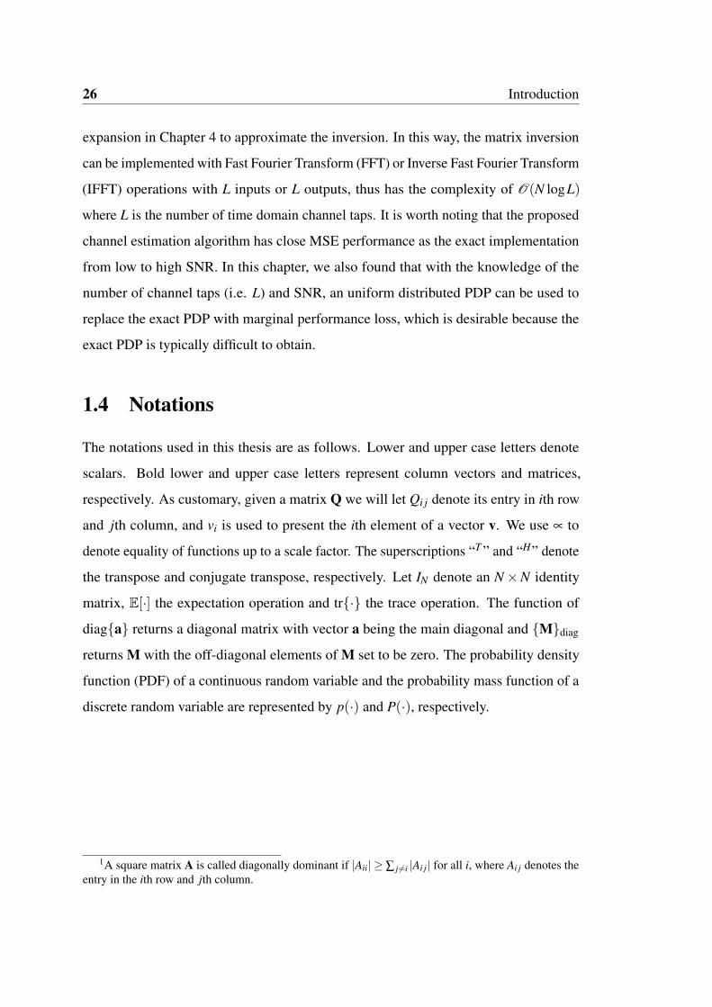
SISO
MMSE Detector
SIS
O D
ec
od
er
n
Interleaver
De-
interleaver-
-
y
La
Le
Fig. 2.2 Iterative Soft-in Soft-Out MMSE Detector
Algorithm 4 Core Part of MMSE-PIC Algorithm in [60]
1: A−1 = (GV+2σ2I)−1 ◃ One matrix inversion per iteration2: for n = 1 to Nt do3: yn = y− ∑
j, j =ng jm j ◃ g j is jth column of G
4: µn = aHn gn ◃ an is the nth row of A−1
5: xn = aHn yn
6: men = xn/µn ◃ extrinsic mean
7: ven = 1/µn − vn ◃ extrinsic variance
8: end for
Table 2.1 Computational Complexity ComparisonPre-computing Every Pass
Algorithm 4 12NrN2
t +NrNt 4N2t +N3
tAlgorithm 3 1
2NrN2t +NrNt 2N2
t +12N3
tAlgorithm 3 1
2NrN2t +NrNt +N3
t 4N2t
2.3.4 Iterative Method to Improve First-pass Performance
By employing SISO MMSE’s soft decision output as its a priori input (see Fig. 2.2),
the SISO MIMO detector itself can run in an iterative manner and we call it iterative
MMSE detection algorithm (I-MMSE). Compared to conventional MMSE turbo receiver,
a 1dB to 2dB performance gain can be obtained. Actually, the fact that self-iteration
can improve system performance had been observed in other literatures [72] [81] where
only one self-iteration has been reported. By contrast, the simulations show that there is
performance gain up to four iterations. More importantly, after employing the proposed

34 A Low Complexity Soft-Decision Feedback MMSE-PIC Detection Algorithm
0 5 10 15 20 25 30
10−4
10−3
10−2
10−1
SNR per receive antenna (dB)
BE
R
Iter0Exact Iter2Approx Iter2Exact Iter4Approx Iter4
4−QAM 16−QAM 64−QAM
Fig. 2.3 BER Performance Comparison Between Exact Implementation and ProposedApproximation for a 16×16 MIMO System.
low complexity matrix inversion, I-MMSE seems more attractive because of its much
lower complexity cost of 4N2t for the second and subsequent pass calculation.
2.4 Simulation Results
2.4.1 Simulation Setup
We consider a Rayleigh slow fading random channel so H does not change over a
codeword. The elements of H are independent and identically Gaussian distributed with
zero mean and variance 1. During simulation, we assume perfect channel information
is available in the detection module. A rate-1/2, regular (3,6) low-density parity-check
(LDPC) code with codeword length of 2000 bits is employed as the channel code and the
maximum number of iterations of the decoder is 25. The square quadrature amplitude

2.4 Simulation Results 35
modulations (2Q-QAM) with Gray mapping are used. For each signal-to-noise (SNR)
value, we run at least 100000 codewords in the Monte Carlo simulations. We set the
scaling factor of output LLR to 0.7 [82]. In the simulations, there are clipping both
in soft-output part and soft-input part of the detector. The soft-in clipping threshold2
for the a priori LLR is ±2, and soft-output module constrains the output LLR range to
[−50,50].
2.4.2 BER Performance
0 5 10 15 20 25 30
10−4
10−3
10−2
10−1
SNR per receive antenna (dB)
BE
R
MMSE−PIC Iter0I−MMSE (1) Iter0I−MMSE (2) Iter0I−MMSE (4) Iter0MMSE−PIC Iter1MMSE−PIC Iter2I−MMSE (1) Iter2I−MMSE (2) Iter2I−MMSE (4) Iter2
4−QAM 64−QAM16−QAM
Fig. 2.4 BER Performance Comparison Between Different Number of Self-iterations for32×32 MIMO.
Fig. 2.3 shows the performance comparison between exact implementation (Algorithm
3) and the proposed approximation (Algorithm 3) of a 16× 16 MIMO system with
4-QAM, 16-QAM and 64-QAM signaling. The legend of Iter=0 stands for the the first2This clipping threshold can also help resolve the numerical stability issue of Line 10 of Algorithm 3
when the a priori variance vn is close to zero.

36 A Low Complexity Soft-Decision Feedback MMSE-PIC Detection Algorithm
pass without the a priori information. The legend of Iter=2 stands for performance
after running two outer loops (between the decoder and the detector). It is clear that
this approximation has nearly no performance loss for 4-QAM signaling, but has small
performance loss for 16-QAM and 64-QAM compared to the exact one. For IDD sys-
tems employing I-MMSE algorithm, there exist two iterative loops. The self-iteration
of detector is the inner loop. The outer loop from the decoder to the detector is the
same as that in a typical turbo system. Through extensive simulation we have found
that the self-iteration method has only marginal performance gain beyond the first outer
pass, thus we only perform the inner loop for the first outer pass. Then we compare
performances between I-MMSE (using Algorithm 3 together with low complexity inner
loop) and the conventional MMSE-PIC (using Algorithm 3) for MIMO systems with
different sizes and various modulation signaling. In Fig. 2.4, the number in the bracket
denotes the number of self-iterations and IterX denotes X outer iterations. It is clear
that the proposed method can significantly improve the first pass system performance
(1dB to 2dB at BER of 10−4). It can also be seen that with more than two self-iterations
there is still performance gain although after four self-iterations the performance gain is
marginal. The simulations show that similar performance gain can also be obtained in
other sized MIMO systems like 16×16 in Fig. 2.5 and 4×4 in Fig. 2.6.
2.5 Conclusion
In this chapter, we firstly employed a low complexity Gaussian model based MMSE
algorithm to perform the MMSE-PIC detection. This algorithm can detect a length-
Nr received data block with only one Hermitian matrix inversion, and the matrix to
be inverted has the size of Nt ×Nt which is especially preferable for massive MIMO
uplink applications where Nt << Nr. Then we proposed a generic method to reduce the
computational complexity of the matrix inversion from O(N3t ) to O(N2
t ) without the
dependence on the size of the random channel matrix. At last, a self-iteration method

2.5 Conclusion 37
0 5 10 15 20 25 30
10−4
10−3
10−2
10−1
SNR per receive antenna (dB)
BE
R
MMSE−PIC Iter0I−MMSE (1) Iter0I−MMSE (2) Iter0I−MMSE (4) Iter0MMSE−PIC Iter1MMSE−PIC Iter2I−MMSE (1) Iter2I−MMSE (2) Iter2I−MMSE (4) Iter2
4−QAM 16−QAM 64−QAM
Fig. 2.5 BER Performance Comparison Between Different Number of Self-iterations for16×16 MIMO.
was proposed to improve a turbo receiver’s first pass performance by 1dB to 2dB with
only a small complexity increase.

38 A Low Complexity Soft-Decision Feedback MMSE-PIC Detection Algorithm
0 5 10 15 20 25 30 35
10−4
10−3
10−2
10−1
SNR per receive antenna (dB)
BE
R
MMSE−PIC Iter0I−MMSE (1) Iter0I−MMSE (2) Iter0I−MMSE (4) Iter0MMSE−PIC Iter1MMSE−PIC Iter2I−MMSE (1) Iter2I−MMSE (2) Iter2I−MMSE (4) Iter2
64−QAM16−QAM
4−QAM
Fig. 2.6 BER Performance Comparison Between Different Number of Self-iterations for4×4 MIMO.

Chapter 3
MIMO Detection Algorithm: Partial
Gaussian Approach with Integer
Programming
3.1 Introduction
As mentioned in Chapter 1, the minimum mean square error parallel interference can-
cellation (MMSE-PIC) algorithm can achieve near optimal performance for massive
MIMO and under well conditioned channels. But high density antennas deployment
may reduce the space between different antennas and thus leads to correlated channel.
The MMSE-PIC algorithm performs poorly under correlated channels. The spatial
correlation between antennas should be taken into account when performing signal
detection.
Recently, we have proposed a Partial Gaussian Approach (PGA) which is very effec-
tive in turbo equalization [45]. The basic idea behind this method is taking M important
symbols as discrete symbols but others as continuous and the continuous symbols can be
assumed to be Gaussian distributed which makes the whole computational complexity
low.
40 MIMO Detection Algorithm: Partial Gaussian Approach with Integer Programming
Channel
Encoder
an MIMO
Modulator
SISO
Decodern
MIM
O D
ete
cto
r
Interleaver
Interle
aver
De-interleaver
...
...
--
bn cn
y
La
Le
Channel
Encoder
MIMO
Modulator
Interle
aver SISO
DecoderInterleaver
De-interleaver-
-
...
Fig. 3.1 Iterative Detection and Decoding of a MIMO Communication System
In this chapter, we investigate the application of PGA for detection of massive MIMO
systems. Simulation results show that under correlated channel PGA has impressive
performance than MMSE-PIC (e.g. under heavily correlated 40×40 MIMO with 16-
QAM signaling, a 5 dB gain can be observed). Due to the marginalization of M discrete
symbols in PGA is exponential in MQ (Q is the number of bits in a symbol), we find that
with larger M (say M ≥ 3) PGA algorithm will have high computational complexity.
In order to reduce the complexity, firstly we apply the “max-log" algorithm and ap-
proximate the APP calculation with the minimization of a quadratic function with integer
variables, thereby reformulating the marginalization problem into a quadratic integer
programming (QIP) problem. Then we implement the depth-first branch-and-bound
algorithm to solve this QIP problem. Simulation results show that the approximation
only causes marginal performance penalty and the proposed branch-and-bound algorithm
has roughly 5% of the exact PGA algorithm’s complexity.
The remainder of this chapter is organized as follows. Section 3.2 describes the
iterative detection system model. Then the Partial Gaussian Approach and the proposed
complexity reduction algorithm are presented in Section 3.3. Simulation results are
shown in Section 3.4.
3.2 System Model
As shown in Fig. 3.1, we consider the uplink of a multiuser MIMO system with Nr
receive antennas at the Base Station and Nt users each with one transmit antenna. The

3.2 System Model 41
received signal in the coded system is represented as
y = Hx+w (3.1)
where y denotes a length-Nr observation vector, H denotes an Nr ×Nt MIMO system
transfer matrix, w denotes a length-Nr circularly symmetric additive white Gaussian
noise (AWGN) vector with PDF N (w;0,σ2I), and x = [x1,x2, · · · ,xNt ]T is mapped
from an interleaved code sequence c, i.e., each xn ∈ A = {α1,α2, · · · ,α2Q}(|A |= 2Q)
corresponds to a length-Q subsequence of c denoted by cn = [cn,1,cn,2, · · ·,cn,Q]T .
The task of the detector is to compute the log-likelihood ratios (LLR) for each code
bit cn,q, which can be expressed as [37]
L(cn,q) = lnP(cn,q = 0|y)P(cn,q = 1|y)
= ln∑xn∈A 0
qP(xn|y)
∑xn∈A 1q
P(xn|y)(3.2)
where A 0q (A 1
q ) denotes the subset of all αi ∈A corresponding to a binary subsequence
with the qth bit given by 0 (1). The extrinsic LLR [17]
Le(cn,q) = L(cn,q)−La(cn,q) (3.3)
will be input to the decoder, where La(cn,q) is the output extrinsic LLR of the decoder in
the last iteration. The key task of the detector is to compute the a posteriori probability
(APP) P(xn|y) for each symbol xn. According to Bayes’ rule, we have
P(xn|y) = ∑x\xn
P(x|y) ∝ ∑x\xn
P(x)P(y|x) (3.4)
where the length-(Nt −1) vector x\xn consists of the elements of x except xn. Given x, y
is Gaussian distributed, i.e., p(y|x) = N (y;Hx,σ2I) (3.4) can then be rewritten as
P(xn|y) ∝ ∑x\xn
P(x)exp[− (y−Hx)H(y−Hx)
σ2
](3.5)

42 MIMO Detection Algorithm: Partial Gaussian Approach with Integer Programming
3.3 Partial Gaussian Approach with Integer Program-
ming
3.3.1 PGA Detection Algorithm
We summarize the PGA detection algorithm [45] in Algorithm 5. After marginalizing
out the contribution from the continuous symbols, the approximate APP of xn in (3.5)
can be represented as the marginalization over M(M ≪ Nt) discrete received symbols as
follows:
P(xn|y) ∝ ∑xD\xn
P(xD)exp[−(xD − z)HZ(xD − z)] (3.6)
where the operation of ∑xD\xncan be performed by enumerating all M data points, and
z and Z are defined in Line 10 and Line 11 in Algorithm 5. It is easy to see that the
total complexity of this marginalization (Line 12) is O(2Q(M+1)), and when M is large
(e.g. larger than 3), it is still too complex for hardware implementation for high order
signaling like 64-QAM.
3.3.2 Simplified Marginalization Calculation
For separable complex symbol constellations such as squared quadrature amplitude
modulation (QAM), the constellation can be separated into two real-valued PAM signals.
Thus we can get a real-valued system model as:
yr = Hrxr +wr (3.7)
where yr = [ℜ(yT ),ℑ(yT )]T , xr = [ℜ(xT ),ℑ(xT )]T , wr = [ℜ(wT ),ℑ(wT )]T and
Hr =
ℜ(H) −ℑ(H)
ℑ(H) ℜ(H)
.
In above equations, ℜ(·) and ℑ(·) represent the real part and the imaginary part
of a complex number, respectively. This way, we can reduce the number of bits in a
modulated symbol to Q = Q2 , thus reduce the complexity.

3.3 Partial Gaussian Approach with Integer Programming 43
As in [60], by ignoring P(xDr ) in (3.6), P(xn|yr) can be approximated by
P(xn|yr) ∝ ∑xD
r \xn
exp[−(xDr − zr)
T Zr(xDr − zr)]. (3.8)
Then, after applying the approximation of ln(ea + eb) ≈ max(a,b) , (3.8) can be
Algorithm 5 Partial Gaussian Approach
Input: y,H,M, La
Output: Le ◃ extrinsic LLR value for every bit1: Calculate a priori mean m and variance V by2: mi = ∑α∈A αP(xi = α)3: Vi = ∑α∈A |α −mi|2 P(xi = α)4: Calculate Vector c and Matrix C by5: C = V−1 + 1
σ2 HHH6: c = C−1[V−1m+ 1
σ2 HHy]7: for n = 1 to Nt do8: Set matrix S by selecting most important M symbols based on HHH [45]9: Calculate Vector z and Matrix Z by
10: Z = (SCST )−1 − (VD)−1
11: z = Z−1[(SCST )−1Sc− (VD)−1mD]12: Calculate P(xn|y) using (3.6) for all xn13: for q = 1 to Q do14: Calculate LLR L(cn,q) using (3.2)15: Calculate Le(cn,q) with (3.3)16: end for17: end for
changed to
P(xn|yr) ∝ exp(−min[(xDr − zr)
T Zr(xDr − zr)]). (3.9)
In Line 12 of Algorithm 5, there are 2Q APP P(xn|yr) should be calculated and each xn
has an enumerated value from the set ˆA = {(2Q −1), · · · ,3,1,−1,−3, · · · ,−(2Q −1)}.
Without loss of generality, we assume that the first variable xD0 of xD
r is the variable of
interest (i.e., xn in (3.8)), thus the scope of the search in the minimizing operation in
(3.9) covers M variables (elements xD1 to xD
M of xDr ).
As each element of xDr (say xD
i ) belongs to the set ˆA , let mi =12(2
Q −1− xi), then
mi ∈ [0,1, · · · ,2Q−1] is the index of the constellation point corresponding to xDi . With a

44 MIMO Detection Algorithm: Partial Gaussian Approach with Integer Programming
little bit of algebra, (3.9) can be reformulated as a quadratic function (after ignoring the
constant factor) as follows:
P(xn|yr) ∝ exp(−min(mT Zm+LT m+C)) (3.10)
where m = [m1, · · · ,mM]T , Z is obtained by deleting the first row and first column of
Algorithm 6 QIP with Branch-and-Bound
Input: Function f (m) = mT Zm+LT m+COutput: Integer vector r minimizing f (m)
1: for d = 1 to M do2: Get Zd by deleting Z’s first d rows and first d columns;3: Calculate the inverse matrices Z−1
d ;4: end for5: m∗ =−1
2(Z−1L); ◃ Minimizing f (m)
6: Set lb = f (m∗); ub = f (r∗); d = 0;7: Rounding m∗ to an initial feasible solution r∗;8: while d ≥ 0 do9: if 0 < d < M then
10: Compute L and C using (3.14);11: Compute m∗ =−1
2(Z−1d L);
12: Set lb = frd(m∗);
13: end if14: if d = M then ◃ Accessing leaf node15: Set lv = f (rM);16: if ub ≥ lv then17: Set r = rM; ub = lv;18: end if19: Set lb = ub;20: end if21: if lb < ub then ◃ Branch on md+122: Set d = d +1; rd = ⌊m∗
1⌉;23: else ◃ Always holds if d = M24: Set d = d −1; ◃ Prune current node25: if d > 0 then ◃ Enumerate next node26: Assign rd based on [83];27: end if28: end if29: end while

3.3 Partial Gaussian Approach with Integer Programming 45
Zr, while C and each element of L can be obtained by:
L j−1 =−M
∑i=0
Z j,iki +2Z0, jxD0 , j ∈ [1, · · · ,M]
C =14
M
∑i=0
M
∑j=0
k jZ j,iki +L0xD0 + xD
0 Z0,0xD0
(3.11)
where ki = 2Q −1− zi with zi representing the ith element of zr and Z j,i is the ( j, i)th
element of matrix Zr.
3.3.3 Resolving QIP with the Branch-and-Bound algorithm
An effective algorithm to handle integer programming is the branch-and-bound algo-
rithm [84]. In our massive MIMO detection application, as the box constraint is typically
not big, e.g. [0,1,2,3] for 16-QAM and [0,1, · · · ,7] for 64-QAM, we select the branching
strategy that consists of fixing a single variable to an integer value in the box constraint
each time. After fixing d variables, we get a reduced function (with M−d variables) as
frd(x) : RM−d → R := f (r1, · · · ,rd,x1, · · · ,xM−d) (3.12)
where {r1, · · · ,rd} (denoted by rd) are the values of those fixed variables. This reduced
function still has a quadratic form of
frd(x) = xT Zdx+ LT x+C (3.13)
where the matrix Zd is obtained from Z by deleting the first d rows and the first d
columns, while C and the elements of the vector L can be calculated by:
C =C+d
∑i=1
Liri +d
∑i=1
d
∑j=1
Zi, jrir j,
L j−d = L j +2d
∑i=1
Zi, jri, j ∈ [d +1, · · · ,M]
(3.14)

46 MIMO Detection Algorithm: Partial Gaussian Approach with Integer Programming
with Zi, j representing the (i, j)th element of Z.
We adopt the well-known Schnorr-Euchner method [83] as enumeration rule and set
the continuous minimum f (x∗) of the reduced function (3.13) as the lower bound. The
initial upper bound is a heuristics based feasible solution, which is a mapping of every
element of m∗ (m∗ =−12(Z
−1L))
to the closest integer in the set of [0,1, · · · ,2Q −1].
Then the upper bound will be tightened after visiting a leaf node with smaller target
function value (Step 4 in Fig. 3.2). When the lower bound is above the upper bound, the
current node will be pruned (Step 5 and 6 in Fig. 3.2) and the next enumeration value
based on the enumeration rule will be attempted. The proposed algorithm is presented in
Algorithm 6.
Fig. 3.2 An example of the proposed branch and bound algorithm where d is the treelevel, lb means low bound, ub means upper bound and m∗ is the vector that minimizesf (m). Because the first heuristic solution happens to be the final solution, there are only6 nodes visited.

3.4 Simulation Results 47
3.4 Simulation Results
3.4.1 Simulation Setup
We use the following correlated complex channel model [85]
H = (RRx)1/2Hw(RT x)
1/2 (3.15)
where RRx and RT x are covariance matrices representing the receive antenna correlation
and transmit antenna correlation, (·)1/2 denote a square root matrix and the elements
of Hw is independent and identically Gaussian distributed with zero mean and variance
one. The channel H is considered as a Rayleigh slow fading channel which means that
H does not change over a codeword. For multiuser uplink application scenario, it is
reasonable to assume that different users are located far away which causes nearly no
transmit side correlation, i.e. RT X = I. We assume
RRx =
1 ρ ρ4 · · · ρ(Nr−1)2
ρ 1 ρ · · · ...
ρ4 ρ 1 . . . ρ4
... . . . . . . . . . ρ
ρ(Nr−1)2 · · · ρ4 ρ 1
(3.16)
where ρ ∈ [0,1] is the fading correlation between two adjacent receive antenna elements
and it is approximated by:
ρ(d)≈ exp(−23 ·△2 ·d2) (3.17)
where △ is the angular spread and d is the distance in wavelengths between the antenna
elements. A rate-1/2, regular (3,6) LDPC code with codeword length 2000 bits is
employed as the channel code. The maximum iteration number of the decoder is 25. The
square 2Q-QAM modulation with Gray mapping is used. During simulation, we assume
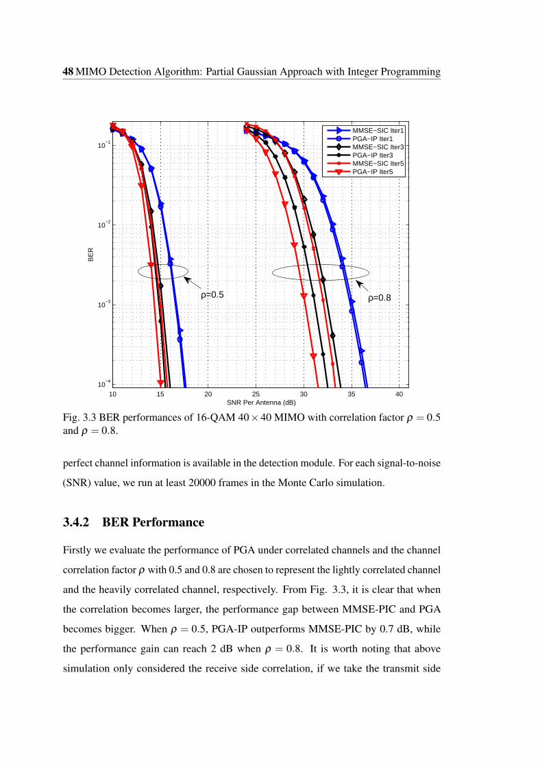
48 MIMO Detection Algorithm: Partial Gaussian Approach with Integer Programming
10 15 20 25 30 35 4010
−4
10−3
10−2
10−1
SNR Per Antenna (dB)
BE
R
MMSE−SIC Iter1PGA−IP Iter1MMSE−SIC Iter3PGA−IP Iter3MMSE−SIC Iter5PGA−IP Iter5
ρ=0.5 ρ=0.8
Fig. 3.3 BER performances of 16-QAM 40×40 MIMO with correlation factor ρ = 0.5and ρ = 0.8.
perfect channel information is available in the detection module. For each signal-to-noise
(SNR) value, we run at least 20000 frames in the Monte Carlo simulation.
3.4.2 BER Performance
Firstly we evaluate the performance of PGA under correlated channels and the channel
correlation factor ρ with 0.5 and 0.8 are chosen to represent the lightly correlated channel
and the heavily correlated channel, respectively. From Fig. 3.3, it is clear that when
the correlation becomes larger, the performance gap between MMSE-PIC and PGA
becomes bigger. When ρ = 0.5, PGA-IP outperforms MMSE-PIC by 0.7 dB, while
the performance gain can reach 2 dB when ρ = 0.8. It is worth noting that above
simulation only considered the receive side correlation, if we take the transmit side

3.5 Conclusion 49
Table 3.1 Average CPU run time (s) comparison between MMSE_PIC, PGA_IP andPGA_Exact for detecting 2000bits with 3 iterations under 40×40 MIMO with 16-QAMon a X86 Linux PC
SNR (dB) 16 17 18 19 20 21 22PGA_EXACT 11.7639 11.7474 11.7556 11.7683 11.7826 11.7798 11.8237
PGA_IP 0.6972 0.6943 0.6874 0.6821 0.6786 0.6779 0.6816MMSE_PIC 0.1158 0.1152 0.1123 0.1083 0.1029 0.0999 0.0983
spatial correlation into account (such as multiple antennas are employed in a single
terminal), PGA-IP has much bigger gain over MMSE-PIC (e.g. 5 dB has been observed
if RT x = RRx and ρ = 0.7). Then, in order to validate the effectiveness of our proposed
PGA-IP algorithm, we compare the BER performance between the PGA-IP and the
exact implementation of PGA. Form Fig. 3.4, it is easily seen that the PGA-IP only
incurs marginal performance loss at the first iteration.
3.4.3 Complexity
PGA in Algorithm 5 is a fixed complexity algorithm, but PGA-IP has a variable com-
plexity because the branch-and-bound algorithm is a kind of data-driven tree search
algorithm. With simulation, we found that the average number of nodes visited is about
8 for every xn of 64-QAM with M = 3 which is much lower than the full search of
23×3 = 512 nodes. From Table 3.1, it is clear that the computational complexity of the
proposed PGA-IP algorithm is much lower than the exact PGA algorithm. We also list
the run time of MMSE-PIC as a reference. We can see that the complexity of PGA-IP
algorithm is only several times higher than the reduced complexity MMSE-PIC which
adopts [17] for iterative MMSE and [38] to reduce the complexity of LLR calculation.
3.5 Conclusion
In this chapter, we have presented the PGA-IP detection algorithm to handle correlated
massive MIMO channel and the simulation results show that it can outperform MMSE-
PIC about 1.5 dB. In order to reduce complexity, a novel algorithm based on Integer

50 MIMO Detection Algorithm: Partial Gaussian Approach with Integer Programming
11 12 13 14 15 16 17 18 19 20 21
10−4
10−3
10−2
10−1
SNR Per Antenna (dB)
BE
R
PGA−Exact Iter1PGA−IP Iter1PGA−Exact Iter2PGA−IP Iter2
Fig. 3.4 BER performance comparison between PGA-Exact and PGA-IP under 16-QAM40×40 MIMO correlated channel (ρ = 0.4)
Programming has been proposed. By computational complexity simulation, we could
see under massive MIMO scenario, PGA-IP detection has nearly the similar complexity
level as the MMSE-PIC algorithm but with better performance.

Chapter 4
A Low Cost LMMSE Channel
Estimator for OFDM Systems
4.1 Introduction
In this chapter, we focus on how to reduce the complexity of the traditional LMMSE
channel estimator for slow fading channels in an OFDM system. The proposed algorithm
can be used in data-aided channel estimation in an iterative system where the estimated
data or decoded data are employed as the virtual pilot. A preamble-type of pilots
based frame structure is employed to provide the initial LMMSE channel estimation.
For the channel estimation, we firstly reformulate the conventional LMMSE channel
estimation to a form that has small sized L×L matrix inversion where L is the number
of non-zero time domain channel taps. Then by exploiting the fact that this small sized
matrix is diagonally dominant due to the law of large numbers, we propose to use
a K terms Neumann series expansion to approximate its inversion. In this way, the
LMMSE estimator can be achieved by a cascade of matrix vector products, which can
be implemented with Fast Fourier Transform (FFT) or Inverse Fast Fourier Transform
(IFFT) operations with L inputs or L outputs, thus has the complexity of O(N logL).
Simulation results show that with small K (K ≤ 2), the performance of the proposed

52 A Low Cost LMMSE Channel Estimator for OFDM Systems
approximation is close to the exact LMMSE implementation from low to high SNR for
both pilot-aided channel estimation and data-aided channel estimation.
The remainder of this chapter is organized as follows. Section 4.2 describes the
OFDM system model. Then the conventional LMMSE channel estimation algorithm is
presented in Section 4.3. In Section 4.4, we propose to use Neumann series expansion to
perform LMMSE channel estimation with low complexity. Simulation results are shown
in Section 4.5 and Section 4.6 concludes this chapter.
4.2 System Model
We consider a coded OFDM system with N subcarriers. The data vector of the nth
OFDM symbol x(n) = [x1,x2, · · · ,xN ]T , which is mapped from an interleaved code
sequence c, i.e., each xi ∈ A = {α1,α2, · · · ,α2Q}(|A |= 2Q) corresponds to a length-Q
subsequence of c denoted by ci = [ci,1,ci,2, · · ·,ci,Q]T , is stacked into one OFDM symbol.
The cyclic prefixes (CP) are inserted before the IFFT of x(n) to ensure the orthogonality
among the subcarriers and prevent inter-symbol interference (ISI) between consecutive
OFDM symbols. Considering a quasi-static channel which is constant during one OFDM
symbol, this OFDM system can be described as a set of parallel additive white Gaussian
noise (AWGN) channels. After dropping the CP and performing FFT, the received
frequency domain signal for OFDM symbol n is given by
y(n) = X(n)η(n)+w(n) (4.1)
where y(n) denotes a length-N observation vector, X(n)≡ diag{x(n)} denotes an N ×
N diagonal matrix with x(n) on its diagonal, η(n) is the frequency domain channel
coefficients and w(n) denotes a length-N circularly symmetric AWGN vector with PDF
C N (w;0,σ2I). For notation simplicity, from now on we omit the time index n.

4.3 LMMSE Channel Estimation 53
The time domain channel coefficients h = [h1,h2, ...,hL]T is related to the frequency
domain channel coefficients η with
η = FLh (4.2)
where FL is a truncated DFT matrix (sized N ×L) with the (k, l)-th element given by
FL(k, l) = exp(− j 2πklN )/
√N with j =
√−1. We assume that the power delay profile
(PDP) of a multipath channel is known1, which can be exploited by the channel es-
timator. The channel coefficients [hi] have zero mean and the covariance E[hhH ] =
diag{p1, ..., pL} ≡ P is regarded as the PDP, where pi is the average power of the i-th
delay path.
4.3 LMMSE Channel Estimation
From (4.1), the LMMSE estimation of frequency domain channel coefficients η can be
computed by [87]
η = CηyC−1yy y (4.3)
where Cηy and Cyy are the covariance matrix of η and y, and the auto-covariance matrix
of y, respectively. Based on the definition of the covariance matrix of two vectors a and
b
Cab = E[(a−E[a])(b−E[b])H], (4.4)
we have
Cηy = CηηXH = NFLPFHL XH (4.5)
and
Cyy = XCηηXH +σ2IN = NXFLPFH
L XH +σ2IN (4.6)
From (4.3), (4.5) and (4.6), it can be seen that directly computing frequency domain
channel coefficients needs an N ×N matrix inversion with O(N3) complexity.
1PDP can also be estimated with low complexity of O(L2)), see [86]

54 A Low Cost LMMSE Channel Estimator for OFDM Systems
Considering that the number of non-zero time domain channel delay taps L can be
much less than the number of subcarriers N, using matrix inversion lemma, (4.3) can be
reformulated to
η = NFLPFHL XH(NXFLPFH
L XH +σ2IN)
−1y
= NFL√
P(N√
PH
FHL XHXFL
√P+σ
2IL)−1√P
HFH
L XHy.(4.7)
As P is a positive definite diagonal real-valued matrix, it is easy to get that√
PH=
√P = diag{√p1,
√p2, · · · ,
√pL}. As a result, (4.7) involves a matrix inversion (sized
L×L) and FFT (IFFT) with computational complexity of O(N logL+L3). At the same
time, by the law of large numbers, it is easy to see that matrix FHL XHXFL is diagonally
dominant, which can be exploited to enable Neumann series expansion to approximate
the matrix inversion, thereby reducing the complexity.
Algorithm 7 LMMSE Channel Estimation for OFDMInput: y,P,X ◃ X is the pilot or feedback dataOutput: η ◃ Frequency domain channel coefficients
1: D = NPtr{XHX}+σ2IL2: v =
√PFH
L XHy3: v0 = D−1v ◃ Initialize Neumann series expansion4: s0 = v05: for i = 1 to K do6: vi = vi−1 −ND−1√PHFH
L XHXFL√
Pvi−1 −σ2D−1vi−17: si = si−1 +vi8: end for9: η = NFL
√PsK
4.4 Newmann Series Expansion Based Channel Estima-
tion
4.4.1 Neumann Series Expansion
Neumann series expansion [88] can be employed to approximate matrix inversion with
the summation of a series of matrix multiplications. For a diagonal dominant matrix M,

4.4 Newmann Series Expansion Based Channel Estimation 55
let D = {M}diag. A K terms Neumann series expansion of M can be written as
M−1 ≈K
∑i=0
(I−D−1M)iD−1. (4.8)
It is easy to see that the multiplication of M−1 and a vector v can be computed by K
loops as
v0 = D−1v, s0 = v0
for i = 1 to K do
vi = (I−D−1M)vi−1
si = si−1 +vi
end for
(4.9)
with M−1v ≈ sK . With (4.9), only matrix-vector multiplications are required, which can
greatly reduce the computational complexity.
4 6 8 10 12 14 16
10−4
10−3
L
MS
E
DPS LMMSE
Dual−Diagonal
Proposed K=1
Proposed K=2
Proposed K=3
Exact LMMSE
Fig. 4.1 MSE performance with different L at SNR of 14dB

56 A Low Cost LMMSE Channel Estimator for OFDM Systems
Let M = N√
PHFHL XHXFL
√P+σ2IL and v =
√PHFH
L XHy and plug them into
(4.9), then (4.7) can be computed by Algorithm 7. In this algorithm, line 1 uses the fact
that {FHL NFL}diag = tr{N}IL for any diagonal matrix N.
4.4.2 Computational Complexity Comparison
In Algorithm 7, the matrices D, X, P are all diagonal. So lines 1, 3, 4, and 7 have
trivial complexity. For Line 2 and Line 9, an IFFT (with L outputs) and an FFT
(with L inputs) can be employed, respectively. Then in Line 6, the computation of
N√
PHFHL XHXFL
√Pvi−1 can be implemented by an FFT with L inputs, followed by an
IFFT with L outputs. In summary, the total complexity of the proposed LMMSE channel
estimation for OFDM system is dominated by 2(K +1) FFTs (or IFFTs) with L inputs
or L outputs. Note that the complexity of FFT or IFFT with L inputs or L outputs can be
computed with complexity of O(N logL) [89].
In [64], the authors have proved that the WDFT based technique [61] [62] [63] can
be treated as special cases of their proposed Dual-Diagonal algorithm. So we focus on
Dual-Diagonal LMMSE algorithm for complexity comparison. For the dual-diagonal
LMMSE algorithm, the frequency domain channel coefficients η = FBFHAy, where
both A and B are diagonal matrices, and F is an N×N DFT matrix, therefore the number
of FFT (IFFT) required is two. Based on the fast algorithm in Appendix I of [64], there
are also two FFTs needed to compute the matrix B. As a result, the total number of N
point FFTs (IFFTs) of the Dual-Diagonal LMMSE algorithm [64] is four, which has the
computational complexity of O(N logN).
4.5 Simulation Results
We consider an OFDM system with N = 128 subcarriers, the carrier frequency is 2.4
GHz and the symbol duration is 0.25 µs. The CP is set to be one-eighth of the number
of subcarriers. The modulation is 64-QAM with Gray mapping. We constrain the total

4.5 Simulation Results 57
0 2 4 6 8 10 12 14 16
10−4
10−3
10−2
10−1
SNR (dB)
MS
E
Proposed K=1
Dual−Diagonal LMMSE
Proposed K=2
Proposed K=3
Exact LMMSE
Fig. 4.2 MSE performance for the 10-tap COST259_RAx channel
transmit power to one, and set the noise variance at receive side to σ2, then the average
received signal-to-noise ratio (SNR) is given by 1/σ2.
4.5.1 Mean-Square Error (MSE) Performance for Time-Invariant
Channels
In order to determine the required minimum K under different channel length, we
select a channel model with the PDP given by pi = Γe−0.1(i−1), i ∈ [1,L] where Γ is
a normalization factor (∑i pi = 1). Fig. 4.1 shows the MSE performance of the exact
LMMSE, the Dual-Diagonal LMMSE [64], the DPS based LMMSE [74]-[76]2 and the
2For the application scenario of this chapter, the DPS algorithm is reduced to one dimension. Thecomplexity of the exact DPS is O(N3). In [76], the complexity is reduced to O(IN) based on space-alternating expectation maximization (SAGE), where I is the number of DPS sequences and is in the orderof L.

58 A Low Cost LMMSE Channel Estimator for OFDM Systems
proposed algorithm with different L at SNR of 14dB. We treat all transmit data as pilot
in order to get the upper bound of the MSE performance.
It is obvious that the proposed algorithm outperforms both the Dual-Diagonal
LMMSE [64] and the DPS based LMMSE [76] even with K = 1. At the same time, for
the proposed algorithm with K = 2, there is small MSE performance loss compared with
the exact LMMSE when L is greater than 8, and with K = 3 the proposed algorithm
has nearly the same performance as the exact LMMSE algorithm for all channel length.
The DPS based LMMSE algorithm has the worst performance as it only requires the
maximum normalized delay spread as the input, but all other algorithms require the
exact channel power profile.
Then we use the 10-tap COST259_RAx [90] channel to compare the MSE per-
formance in Fig. 4.2. It can be seen that the proposed method has nearly the same
performance as the exact LMMSE with K = 3 while there is small performance loss in
high SNR region with K = 2. It is also obvious that even with K = 2 the proposed algo-
rithm outperforms the Dual-Diagonal LMMSE algorithm and the DPS based LMMSE
algorithm from low to high SNR range.
4.5.2 Bit Error Rate (BER) Performance for Iterative Systems
As in Section V.A of [26], we consider an iterative channel estimation scheme, where
the hard decision from the output of the channel decoder is employed as the virtual
pilot. We employ a frame structure that every frame contains 25 OFDM symbols and
the first symbol is the pilot symbol to provide the initial LMMSE channel estimation
for the iterative channel estimation scheme3. With slow fading assumption, the channel
coefficients of the last OFDM symbol are used for the current symbol detection, then
the hard decision fed back from the decoder is mapped to a data symbol, which is
exploited to update the channel estimation. Although we assume that the channel is
static within one OFDM symbol in the design of the channel estimation, the channel
coefficients generated in the simulations changed at every sampling time according to
Jakes model [91] and the received singal was generated using the time-varying channel.

4.5 Simulation Results 59
11 12 13 14 15 16 17 18
10−4
10−3
10−2
10−1
SNR (dB)
BE
R
DPS Iter0
DPS Iter1
Dual−Diagonal Iter0
Proposed Iter0
Exact LMMSE Iter0
Dual−Diagonal Iter1
Proposed Iter1
Exact LMMSE Iter1
Fig. 4.3 BER performance for 10-tap COST259_RAx Channel at speed of 100 km/hour
For the Jakes model, the relative speed between the transmitter and the receiver is
assumed to be 100 km/hour. In the simulations, we used the 10-tap COST259_RAx
channel model [90]. A rate-1/2, regular (3,6) low-density parity-check (LDPC) code
with codeword length of 768 bits was also used. For the LDPC decoder, the maximum
number of iterations between the variable nodes and the check nodes was 25.
Fig. 4.3 shows the BER performance of the system with exact LMMSE, Dual-
Diagonal LMMSE [64], DPS based LMMSE [76] and the proposed LMMSE approx-
imation. It is clear that the proposed algorithm with K = 2 nearly has the same BER
performance as the exact LMMSE algorithm and always better than the Dual-Diagonal
method and the DPS based LMMSE algorithm.
3Besides the preamble-type pilot in our example, the proposed algorithm can be easily applied to othertypes of pilots.

60 A Low Cost LMMSE Channel Estimator for OFDM Systems
4.6 Discussion
4.6.1 The Power Delay Profile (PDP)
For the LMMSE channel estimation algorithm, there is a limitation that it requires the
PDP as a input which is typically difficult to obtain. This means that the PDP exploited
in the proposed algorithm may not be the same as that experienced by the transmit signal.
But fortunately, we have found that with the knowledge of the number of channel taps
(i.e. L) and SNR only, we can get close MSE performance to the exactly known PDP
case by artificially using an uniform distributed PDP for the proposed algorithm.
In order to validate this result under different channels, we have simulated the
channel models shown in Table 4.1 and the MSE performances are shown in Fig. 4.4. In
the simulations, the uniform PDP is defined as pi = 1/L, i ∈ [1, ...,L], the exponential
PDP 1 is defined as pi = Q1e−0.1(i−1), i ∈ [1, ...,L] where Q1 is a normalization factor
(∑i pi = 1), and the exponential PDP 2 is defined as pi = Q2e−0.5(i−1), i ∈ [1, ...,L] where
Q2 is also a normalization factor. Fig. 4.4 shows the MSE performance comparison
between the exact PDP, the uniform PDP, the exponential PDP 1 and the exponential
PDP 2 under different channel models. It is easy to see that the uniform PDP nearly has
the same MSE performance as the exact PDP.
It is worth noting that the above finding was also reported and analysed in [92]
4.6.2 The Assumption of Quasi-static Channel
While we assume that the channel is static within one OFDM symbol in the design of
the channel estimation, the channel coefficients generated in the simulations changed
at every sampling time according to Jakes model. Thus the maximum Doppler spread
normalized by the duration of one OFDM symbol is an important design factor for
our proposed channel tracking scheme to work properly. If this Doppler spread is too
big, there is too big difference between the channel coefficients of two subsequent
OFDM symbols and thus the channel tracking mechanism will fail. The Doppler spread

4.7 Conclusion 61
Table 4.1 Simulated Channel Models [2]No. Channel Model PDP in dB
1COST259_RAx
Rural ara, 10-tap channel3GPP_TR_25.943
−5.2−6.4−8.4−9.3−10−13.1−15.3−18.5−20.4−22.4
2COST207_TU12
Typical urban, 12-tap channel−4−30−2.6−3−5−7−5
−6.5−8.6−11−10
3COST207_HT
THilly terrain, 6-tap channel 0−2−4−7−6−12
4ITU_Vehicular_A
ITU Vehicular A, 6-tap channel 0−1−9−10−15−20
5ITU_Pedestrian_A
4-tap channel 0−9.7−19.2−22.8
6ITU_Pedestrian_B
6-tap channel 0−0.9−4.9−8−7.8−23.9
normalized by the duration of one OFDM symbol can be calculated by:
fdmax =vmax fC
c0Ts
=vmax fC
c0(N +NCP)Tsample
(4.10)
where vmax is the maximum movement speed, c0 = 3.0×10⁸m/s is the speed of light, fC
is the carrier frequency, Ts is the OFDM symbol length, N is the number of subcarriers,
NCP is the length of CP and Tsample is the sample rate. For above simulations, for
vmax = 100 km/h the the Doppler spread normalized by the duration of one OFDM
symbol is 0.008.
4.7 Conclusion
In this chapter, we have proposed a low complexity LMMSE channel estimation algo-
rithm for OFDM systems by approximating the matrix inversion with Neumann series
expansion. This enables the channel estimation to be implemented with L-point input
FFT or L-point output IFFT, which have the complexity of O(N logL). Extensive sim-
ulation results show that under different channel models, the proposed algorithm can

62 A Low Cost LMMSE Channel Estimator for OFDM Systems
0 5 10 15
10−4
10−3
10−2
10−1
Channel NO.6
Channel NO.6Channel NO.6
0 5 10 15
10−4
10−3
10−2
10−1
Channel NO.5
Channel NO.5Channel NO.5
0 5 10 15
10−4
10−3
10−2
10−1
Channel NO.4
Channel NO.4Channel NO.4
0 5 10 15
10−4
10−3
10−2
10−1
Channel NO.3
Channel NO.3Channel NO.3
0 5 10 15
10−4
10−3
10−2
10−1
Channel NO.2
Channel NO.2Channel NO.2
0 5 10 15
10−4
10−3
10−2
10−1
Channel NO.1
Channel NO.1Channel NO.1
Exact
Uniform
Exp 1
Exp 2
Exact
Uniform
Exp 1
Exp 2
Exact
Uniform
Exp 1
Exp 2
Exact
Uniform
Exp 1
Exp 2
Exact
Uniform
Exp 1
Exp 2
Exact
Uniform
Exp 1
Exp 2
Fig. 4.4 MSE Under Channel No.1-6
achieve good MSE performance from low to high SNR range, and nearly the same
BER performance as the exact LMMSE algorithm. We also found that using a uniform
distributed PDP only incurs marginal performance loss but can relaxing the requirement
from the exact PDP to the maximum number of time domain channel taps.
Chapter 5
Low Complexity Iterative MMSE-PIC
Detection for Medium-Size Massive
MIMO
5.1 Introduction
When the number of receive antennas at the base station becomes large, in particular,
much larger than the number of total transmit antennas in user terminals, a simple
detection algorithm such as a matched filter can achieve very good performance, as
with the assumption of i.i.d. entries for channel matrix H, the channel vectors become
orthogonal to each other and HHH converges to a scaled identity matrix. But for practical
medium-size massive MIMO, matched filter based detection algorithm suffers perfor-
mance loss [72]. Therefore, alternative linear detection algorithms such as the minimum
mean square error parallel interference cancellation (MMSE-PIC) algorithm [60] are
often employed due to their relatively low complexity and good bit error rate (BER) per-
formance. However, the MMSE-PIC still requires complexity of O(K3) for calculating
a matrix inversion and O(K2M) for calculating the Gram matrix, where K is the number
of transmit antennas and M is the number of receive antennas.
64 Low Complexity Iterative MMSE-PIC Detection for Medium-Size Massive MIMO
To reduce the complexity, [70] and [71] employed Neumann series expansion to
approximate the matrix inversion by a matrix polynomial. Then in [72] the authors
proposed to use the same method to perform 3GPP-LTE uplink signal detection and
proved the convergence of the Neumann series expansion. Different from using Neumann
series expansion, in [1] an iterative method based on successive overrelaxation (SOR)
is employed to calculate the product of the inversion of a matrix and a vector, which
can converge to the exact solution. These work can successfully reduce the complexity
of computing matrix inversion from O(K3) to O(K2). But they all require the pre-
computed Gram matrix as an input. In massive MIMO with M ≫ K, the Gram matrix
computation involves computational complexity of O(K2M), which is much higher than
the O(K3) complexity of matrix inversion .
In this chapter, based on the MMSE detection algorithm [17], we exploit Neumann
series expansion to reduce the total complexity of MMSE-PIC for massive MIMO. With
the proposed method, computational complexity is reduced by avoiding direct matrix
inversion and replacing the matrix-matrix multiplication of Gram matrix with matrix-
vector multiplications. Specifically, we propose to employ an L (typically L ≤ 3) terms
Neumann series expansion for calculating the means of data symbols to be detected, and
a first order approximation for calculating the variances and thus reducing the complexity
from O(K2M+K3) to O(LKM) with marginal performance loss when L = 3 for MIMO
size of K×M = 16×128. We also investigate the application of the proposed algorithm
in an iterative detection and decoding (IDD) system, where the symbol detector and the
channel decoder work iteratively. We found that with one iteration between the decoder
and the detector, the proposed approximation algorithm with L = 3 can achieve the same
performance as the exact MMSE-PIC algorithm.
The remainder of this chapter is organized as follows. Section 5.2 describes the
turbo-MIMO system model. Then in Section 5.3, we propose to use Neumann series
expansion to perform MMSE detection without computing the Gram matrix. Simulation
results are shown in Section 5.4 and Section 5.5 concludes this chapter.

5.2 System Model 65
5.2 System Model
Consider a multiuser massive MIMO system with M receive antennas at the base station
and K single-antenna user terminals. Let x = [x1,x2, . . . ,xK]T denote the transmit vector
comprising the symbols transmitted simultaneously by all users in one channel use where
xn ∈ A = {α1,α2, . . . ,α2Q}(|A |= 2Q) denotes transmitted symbol from user n, then
each xn corresponds to a length-Q subsequence of c denoted by cn = [cn,1,cn,2, · · ·,cn,Q]T.
Let H = [h1,h2, . . . ,hK] denote the channel gain matrix, where hn = [h1n,h2n, . . . ,hMn]T
is the channel gain vector from user n to the base station, and h jn denotes the channel
gain from the n-th user to the j-th receive antenna at the base station. Assuming rich
scattering, adequate spatial separation between the base station antenna elements and
perfect user power control, h jn,∀ j are assumed to be i.i.d. complex Gaussian distributed
with zero mean and variance one. Thus a length-M observation vector y at the base
station can be written as
y = Hx+w (5.1)
where w denotes a length-M circularly symmetric additive white Gaussian noise (AWGN)
vector with zero-mean and covariance of σ2I.
The task of the Soft-In Soft-Out (SISO) detector is to compute the extrinsic log-
likelihood ratio (LLR) for each code bit cn,q, which is the input to the decoder and can
be expressed as [17]
Le(cn,q) = ln
∑xn∈A 0
q
P(y|xn)P(xn)
∑xn∈A 1
q
P(y|xn)P(xn)−La(cn,q) (5.2)
where La(cn,q) is the output extrinsic LLR of the decoder, xn ∈ A 0q (A
1q ) represents
constellations whose q-th bit is 0(1) and P(xn) is the a priori probability of xn which
can be calculated from La(cn,q).

66 Low Complexity Iterative MMSE-PIC Detection for Medium-Size Massive MIMO
5.3 MMSE Detection Based on Neumann Series Expan-
sion
We employ the method proposed in [17] to perform MIMO MMSE detection. With
this algorithm, it is easy to reformulate the matrix to be inverted with the size of K ×K
which is preferable for massive MIMO applications with M ≫ K. The core part of this
algorithm is to compute the a posteriori mean mp and variance Vp of x by
Vp = (V−1 +1
σ2 HHH)−1, (5.3)
mp = m+1
σ2 Vp(HHy−HHHm), (5.4)
where m and V are the a priori mean and variance of x, respectively, and they can be
calculated from the feedback of the decoder1. Then the extrinsic mean men and variance
ven of the n-th element of x (which are used to generate soft-out LLR) can be calculated
by
ven = (
1vp
n− 1
vn)−1, (5.5)
men = ve
n(mp
n
vpn− mn
vn), (5.6)
where vn, vpn are the (n,n)-th elements of matrix V and Vp, respectively, and mn, mp
n are
the n-th elements of vector m and mp, respectively. It is easy to see that (5.3) and (5.4)
require a computational complexity of O(K2M) for calculating HHH and O(K3) for
calculating the matrix inverse.
1At the beginning of the IDD, there is no feedback from the decoder. Assuming that the constellationof the modulation is with zero mean and normalized with unit power and data streams from differenttransmit antennas are statistically independent, we have m be a zero vector and V be the identity matrixIK with size K ×K.

5.3 MMSE Detection Based on Neumann Series Expansion 67
Algorithm 8 Reduced Complexity Neumann Series expansion based MMSE detection
Input: y, H, La
Output: Le ◃ extrinsic LLR value for every bit1: Calculate a priori mean m and variance V from La
2: mn = ∑αi∈A
αiP(xn = αi)
3: vn = ∑αi∈A
|αi −mn|2 P(xn = αi)
4: Calculate a posteriori mean mp
5: D = diag(V−1 + 1σ2 HHH)
6: v0 = D−1(HHy−HHHm)7: s0 = v08: for i = 1 to L do9: vi = vi−1 −D−1(V−1 + 1
σ2 HHH)vi−110: si = si−1 +vi11: end for12: mp = m+ 1
σ2 sL13: Approximate the diagonal elements of Vp
14: vpn = dn ◃ dn is the (n,n)-th element of D−1
15: Calculate extrinsic mean men and variance ve
n16: ve
n = ( 1vp
n− 1
vn)−1
17: men = ve
n(mp
nvp
n− mn
vn)
18: Calculate extrinsic LLR Le
19: Le(cn,q) = ln∑
αi∈A 0q
exp(− |αi−me
n |2ven
)∏
q′ =q
P(cn,q′
=si,q′
)
∑
αi∈A 1q
exp(− |αi−me
n |2ven
)∏
q′ =q
P(cn,q′
=si,q′
)

68 Low Complexity Iterative MMSE-PIC Detection for Medium-Size Massive MIMO
5.3.1 Neumann Series Expansion
The convergence of Neumann series expansion for detection has been proved in [72]. It
has been shown in [72] that, for large ρ = M/K, the Gram matrix G = HHH tends to be
diagonally dominant, which enables the convergence of the Neumann series expansion.
Let us decompose the regularized Gram matrix A = V−1+ 1σ2 G to A = D+E, where
D is the main diagonal of A. As V is a diagonal matrix, the complexity of computing D
is the same as computing the diagonal elements of G. We can then approximate A−1 in
the Neumann series as
A−1 ≈L
∑i=0
(IK −D−1A
)iD−1
=L
∑i=0
(IK −D−1V−1 − 1
σ2 D−1G)iD−1.
(5.7)
Using A−1 of (5.7) to replace Vp and plugging it into the representation of mp of (5.4),
it can be seen that only matrix-vector multiplications are needed for calculating mp and
the calculation of the Gram matrix G itself is avoided. But we should note that in (5.5)
and (5.6) the diagonal elements of Vp are also required to compute the extrinsic mean
and variance. To reduce the complexity, we propose to use the first order approximation
(L = 0) of (5.7) for computing the diagonal elements of Vp (i.e. Vp ≈ D−1).
From (5.7), it is obvious that the multiplication of A−1 and a vector v can be
computed by L loops. The proposed MIMO MMSE detection algorithm with Neumann
series expansion is summarized in Algorithm 8. We note that when L = 0, the proposed
algorithm coincides with the matched filter detector as mp = 1σ2 D−1HHy (Note that we
assume m is a zero vector at the beginning of IDD).
5.3.2 Computational Complexity Comparison
We focus on the number of real-valued multiplications needed and only count quadratic
or beyond terms. For the real-valued system model, the matrix size of H is 2K×2M, y is
a length-2M vector and m is a length-2K vector. Note that using the symmetric property

5.4 Simulation Results 69
of matrix G and Vp can reduce the complexity by a half. Table 5.1 is a summary
of complexity comparison between MMSE, the proposed algorithm, Neumann series
expansion based algorithm in [70] and SOR based algorithm in [1]. In the table, the
term 4K2M corresponds to the computing of Gram matrix G. Note that for SOR based
algorithm in [1], the number of iterations Ls may be smaller than that of Neumann series
expansion.
Table 5.1 Computational Complexity ComparisonAlgorithm Number of multiplicationsExact MMSE [17] 8K2 +4K3 +4(K2 +K)MProposed (16+8L)KMNeumann series based [70] 4K2M+8(L−2)K3
SOR based [1] 4K2M+4LsK2
5.3.3 Discussion
In contrast to [70], [71], and [72], which also use the Neumann series expansion to
approximate matrix inversion, the proposed methods avoid direct matrix inversion and
replace the matrix-matrix multiplication by matrix-vector multiplications, which result
in considerable saving in computations.
The method proposed in [1], after optimizing a parameter by off-line exhaustive
searching, can converge faster than Neumann series expansion. But it requires each
element of matrix G as its input, which means that HHH has to be computed explicitly,
thus it cannot reduce the total complexity significantly.
5.4 Simulation Results
We consider a Rayleigh block fading random channel where H does not change over a
codeword. During simulations, we assume that perfect channel information is available
in the detection module. A rate-1/2, regular (3,6) low-density parity-check (LDPC) code
with codeword length of 2000 bits is employed as the channel code and the maximum
number of iterations of the decoder is 25. The constellation of 64-QAM with Gray

70 Low Complexity Iterative MMSE-PIC Detection for Medium-Size Massive MIMO
−2 −1.5 −1 −0.5 0 0.5 1 1.5 2
10−4
10−3
10−2
10−1
SNR per receive antenna (dB)
BE
R
Proposed (L=0)Proposed (L=0) VarProposed (L=1)Proposed (L=1) VarProposed (L=2)Proposed (L=2) VarSOR (L
s=2)
Proposed (L=3)Proposed (L=3) VarExactProposed (L=3) IDD
Fig. 5.1 BER performance comparison for exact MMSE, proposed and SOR based [1]with MIMO size of K ×M = 16×128
mapping is used. We constrain the total transmitter power to one, and set the noise
variance at each receive antenna to σ2. Then the average received signal-to-noise ratio
(SNR) at each receive antenna is given by 1/σ2. For each SNR value, we simulate at
least 100000 codewords. In the simulations, clipping is applied to both the soft-output
and the soft-input of the detector. The soft-in clipping threshold2 for the a priori LLR is
±2, and soft-output module constrains the output LLR range to [−50,50].
Fig. 5.1 shows the BER performance comparison between the exact MMSE detec-
tion [17], the proposed algorithm and the SOR based algorithm [1]. The MIMO size
is K ×M = 16×128. It is easy to see that the performance of the matched filter (with
legend Proposed (L=0)) is poor. At the same time, with a larger L the approximation is
more accurate and when L = 3 the proposed algorithm can approach the performance
2This clipping threshold can also help resolve the numerical stability issue of Line 16 and Line 17 ofAlgorithm 8 when the a priori variance vn is close to zero.

5.5 Conclusion 71
of the exact algorithm within 0.3dB. It can also be seen that an extra IDD iteration
(with legend Proposed (L=3) IDD) achieves slightly better performance than the exact
MMSE-PIC algorithm without IDD.
To evaluate the performance loss caused by the first order approximation of Vp, we
use (5.7) to explicitly compute the matrix inversion and assign the diagonal elements
to vpn (as in [70]) and the performances are shown in Fig. 5.1 with legends ending with
Var. It is obvious that the proposed approximation to variance only leads to a small
performance penalty.
5.5 Conclusion
In this chapter, we have proposed to use Neumann series expansion to reduce the
complexity of the MMSE-PIC algorithm for massive MIMO applications with M ≫
K. Firstly, an L terms Neumann series was employed to avoid computing the matrix
inversion by replacing it with a cascade of matrix-vector multiplications. Then, a first-
order approximation was employed to compute the diagonal elements of the a posteriori
variance matrix for calculating LLR, which helps to avoid computing the Gram matrix
explicitly. Simulation results showed that with a small L the proposed approximation
methods lead to marginal performance loss compared with the exact implementation,
but with considerable complexity saving.


Chapter 6
A Novel Interpolation Algorithm for
Massive MIMO OFDM System
Detection
6.1 Introduction
The aforementioned detection algorithms can be applied to flat-fading channels (e.g.
signal detection at each subcarrier of an OFDM system). In this chapter, we will focus
on the detection of all subcarriers of a massive MIMO-OFDM system. As the number of
subcarriers N in a MIMO-OFDM system is typically large, the receiver will have very
high computational complexity if we apply the aforementioned algorithms for every
subcarrier.
In OFDM systems, as the frequency domain coefficients are typically highly corre-
lated, interpolation is often employed to reduce the complexity. For MMSE detection,
the matrix inversion is the main contributor to the complexity. There are several works
which use the interpolation method to compute the matrix inversion. For example, [93]
and [94] exploited the fact that the adjoint and the determinant of a matrix can be repre-
sented in a polynomial form and thus they can be interpolated. Then based on the results
of [93] and [94], [95] proposed a Gaussian approximation for phase shifted interpola-
74 A Novel Interpolation Algorithm for Massive MIMO OFDM System Detection
tion method. Recently, [96] proposed a Banachiewicz formula based matrix inversion
with low complexity. But all these interpolation based algorithms were designed for
small-size MIMO and cannot be easily extended to massive MIMO applications.
In this chapter, from the asymptotic property of Gram matrix we conjecture that
there might be strong correlation between the (regularized) Gram matrix inversions of
adjacent subcarriers for medium-size massive MIMO, which was verified by simulations.
By exploiting this strong correlation, we proposed a linear interpolation based MMSE
detection algorithm which can significantly reduce the number of matrix inversion
required. Extensive simulations show that with the same level of complexity as the
matched filter, the proposed algorithm only incurs small BER performance loss compared
to the exact MMSE detector.
The remainder of this chapter is organized as follows. Section 6.2 describes the
massive MIMO-OFDM system model and soft output MMSE detection algorithm.
Then in Section 6.3, the strong correlation of the matrix inversion for massive MIMO is
evaluated and a linear interpolation algorithm is proposed to compute the matrix inversion
with low complexity. Simulation results are shown in Section 6.4 and conclusion is
given in Section 6.5.
6.2 System Model and Soft-output MMSE Detector
Considering a coded massive MIMO-OFDM system with Nr receive antennas, Nt trans-
mit antennas and N subcarriers, the multipath channel can be mapped to N flat-fading
channels. For subcarrier n = 1, . . . ,N, the received signal at the base station can be
modelled as
yn = Hnxn +wn (6.1)
where yn denotes a length-Nr observation vector, Hn denotes an Nr ×Nt MIMO system
transfer matrix of subcarrier n, wn denotes a length-Nr circularly symmetric additive
white Gaussian noise (AWGN) vector with zero means and covariance of σ2I, and xn =
[x1,x2, . . . ,xN t]T is the data symbol vector transmitted on subcarrier n which is mapped

6.2 System Model and Soft-output MMSE Detector 75
from an interleaved code sequence c, i.e., each xi ∈ A = {α1,α2, . . . ,α2Q}(|A |= 2Q)
corresponds to a length-Q subsequence of c denoted by ci = [ci,1,ci,2, . . . ,ci,Q]T .
The task of a soft-output detector is to compute the extrinsic log-likelihood ratio
(LLR) for each code bit. We apply the LMMSE algorithm in [17] to the MIMO detection.
As we only concern the conventional MMSE detection, after setting V = INt and m a
zero vector, the a posteriori mean mp and variance Vp of x can be calculated by [17]
Vpn = (INt +
1σ2 HH
n Hn)−1, (6.2)
mpn =
1σ2 Vp
nHHn yn, (6.3)
Then the extrinsic mean men,i and variance ve
n,i of the i-th element of xn can be calculated
by
ven,i = (
1vp
n,i−1)−1, (6.4)
men,i = ve
n,imp
n,i
vpn,i
, (6.5)
where vpn,i is the (i, i)-th element of matrix Vp
n and mpn,i is the i-th element of vector mp
n,
respectively. At last, the LLR can be calculated by:
Le(ci,q) = ln
∑α j∈A 0
q
exp(− |α j−me
n,i|2ve
n
)∑
α j∈A 1q
exp(− |α j−me
n,i|2ve
n,i
) (6.6)
where α j ∈ A 0q (A
1q ) represents constellations whose q-th bit is 0(1). It is worth noting
that (6.6) can be simplified by exploiting the constellation regularity [38]. It is easy to
see that (6.2) and (6.3) require computational complexity of O(N2t Nr) for calculating
HHH and O(N3t ) for calculating the matrix inversion.

76 A Novel Interpolation Algorithm for Massive MIMO OFDM System Detection
6.3 MMSE Detection Based on Interpolation
It is obvious that with large number of subcarriers N, the brute-force tone-by-tone
detection incurs prohibitive complexity. To reduce the complexity, one method is to
exploit the correlation between adjacent subcarriers to compute matrix inversion by
using interpolation. This idea was investigated in several works [93]-[96]. In [93], [94]
and [95], interpolation based matrix inversion algorithms were proposed by employing
the fact that even though the inverse of a polynomial matrix is generally not polynomial,
the adjoint and the determinant is polynomial, which allows efficient inversion of the
individual matrices through interpolation. But as mentioned in [93] and [94], these
methods are only useful for limited matrix size as the adjoint matrix is difficult to obtain
for arbitrary matrix size. In [96], an interpolation based matrix inversion algorithm based
on Banachiewicz formula for the inverse of a partitioned matrix was proposed for 4×4
MIMO. But this algorithm is difficult to be extended to massive MIMO applications.
In this section, by theoretical analysis and simulation results we will show that
the matrix inversion of Gram matrix required by a zero forceing (ZF) detector or a
regularized Gram matrix required by an MMSE detector has strong correlation between
adjacent subcarriers for massive MIMO-OFDM systems. Then we will propose a low
complexity detection algorithm which computes the inversion matrix from the base tones
by linear interpolation.
6.3.1 Correlation of Matrix Inversion for Massive MIMO-OFDM
Systems
It is well known that for massive MIMO where Nt ≪ Nr, the Gram matrix Gn = HHn Hn
becomes a diagonally dominant matrix and approaches a scaled identity matrix when
both Nt and Nr approach infinite. This implies that the matrix inversions G−1n of adjacent
subcarriers have the strongest correlation when Nt and Nr approach infinite. This fact
inspires us to consider that when Nt and Nr are not so big, there should still be some
correlation between G−1n of adjacent subcarriers. In the following, we use simulation

6.3 MMSE Detection Based on Interpolation 77
−10 −5 0 5 100.5
0.55
0.6
0.65
0.7
0.75
0.8
0.85
0.9
0.95
1
d
Cor
rela
tion
Channel Correlation Ch(d)
Correlation Cg(d) ρ=6
Correlation Cg(d) ρ=8
Correlation Cg(d) ρ=10
Correlation Cg(d) ρ=12
Fig. 6.1 Correlations of Ch(d) and Cg(d) of adjacent subcarriers with N = 64, Nt = 20,different ρ and different subcarrier distance d.
to confirm this conjecture. As in [97], the channel correlation coefficients between
subcarrier n and subcarrier n+d (assuming modulo addition) are defined as
Ch(d) =E[|hH(n+d)h(n)|2
]√E[||hH(n+d)||2
]E[||h(n)||2
] (6.7)
where h(n) = vec(Hn) is the vector obtained by stacking the columns of Hn one on top
of the other, and n ∈ [1,N].

78 A Novel Interpolation Algorithm for Massive MIMO OFDM System Detection
Similarly, the correlation coefficients between G−1n and G−1
n+d can be defined as
Cg(d) =E[|gH(n+d)g(n)|2
]√E[||gH(n+d)||2
]E[||g(n)||2
] . (6.8)
where g(n) = vec(G−1n ).
Fig. 6.1 shows the correlations Ch(d) and Cg(d) under different subcarrier distance d
for different sized MIMO (Nt = 20 and with different ρ =Nr/Nt) with N = 64 subcarriers.
It is obvious that when the distance d becomes larger the correlations of Ch(d) and Cg(d)
decreases accordingly as expected. On the other hand, the correlation Cg(d) between
adjacent tones drops much slower than Ch(d) does. At the same time, the correlation
coefficient dropping rate (according to the increased d) is smaller for massive MIMO
systems with bigger ρ than those with smaller ρ .
Table 6.1 Simulated Channel Models [2]No. Channel Model Delay in ns
1COST207_TU6alt
Alt typical urban 6-tap 0 200 500 1600 2300 5000
2COST259_RAxRural ara, 10-tap
3GPP_TR_25.943
0 42 101 129 149245 312 410 469 528
3COST207_TU12
Typical urban, 12-tap0 200 400 600 800 1200 1400
1800 2400 3000 3200 5000
4COST207_HT
THilly terrain, 6-tap 0 200 400 600 15000 17200
5ITU_Pedestrian_A
ITU Pedestria A, 4-tap 0 110 190 410
6ITU_Vehicular_A
ITU Vehicular A, 6-tap 0 310 710 1090 1730 2510
In order to evaluate the correlations under different channel models, the correlations
of Ch(d) and Cg(d) of adjacent subcarriers are simulated for the channels listed in Table
6.1 and the results are shown in Fig. 6.2.
From this figure, it is clear that for the channels with small L (taps of time domain
coefficients), the correlations of both Ch(d) and Cg(d) between adjacent subcarriers
are large. For channels with the same L (like channel No. 2, No. 3 and No. 4), the
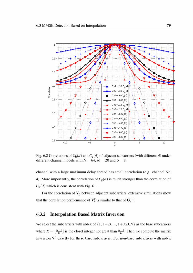
6.3 MMSE Detection Based on Interpolation 79
−10 −5 0 5 100.3
0.4
0.5
0.6
0.7
0.8
0.9
1
d
Cor
rela
tion
Ch2−L10 Ch(d)
Ch2−L10 Cg(d)
Ch1−L6 Ch(d)
Ch1−L6 Cg(d)
Ch3−L12 Ch(d)
Ch3−L12 Cg(d)
Ch4−L6 Ch(d)
Ch4−L6 Cg(d)
Ch5−L4 Ch(d)
Ch5−L4 Cg(d)
Ch6−L6 Ch(d)
Ch6−L6 Cg(d)
Fig. 6.2 Correlations of Ch(d) and Cg(d) of adjacent subcarriers (with different d) underdifferent channel models with N = 64, Nt = 20 and ρ = 8.
channel with a large maximum delay spread has small correlation (e.g. channel No.
4). More importantly, the correlation of Cg(d) is much stronger than the correlation of
Ch(d) which is consistent with Fig. 6.1.
For the correlation of Vp between adjacent subcarriers, extensive simulations show
that the correlation performance of Vpn is similar to that of G−1
n .
6.3.2 Interpolation Based Matrix Inversion
We select the subcarriers with index of {1,1+D, ...,1+KD,N} as the base subcarriers
where K = ⌊N−1D ⌋ is the closet integer not great than N−1
D . Then we compute the matrix
inversion Vp exactly for these base subcarriers. For non-base subcarriers with index

80 A Novel Interpolation Algorithm for Massive MIMO OFDM System Detection
inside the range (1,1+KD), the matrix inversion can be computed by linear interpolation
asVp
kD+1+d = (1− dD)Vp
kD+1 +dD
Vp(k+1)D+1,
d ∈ (1,D) and k ∈ (0,K).
(6.9)
For the subcarriers with index between 1+KD and N, the matrix inversion can be
computed by linear interpolation as
VpKD+1+d = (1− d
D1)Vp
KD+1 +d
D1Vp
N ,
d ∈ (1,D1)
(6.10)
where D1 = N −KD−1.
6.3.3 Computational Complexity Comparison
We focus on the number of complex-valued multiplications needed and only count
quadratic or beyond terms. Note that the symmetric property of matrix Gn and Vpn can
be exploited to reduce the complexity by a half. We use the complexity of matched filter
as the benchmark which has the complexity of O(NrNt) for every tone. We choose [17]
for exact implementation for base tones and using interpolation of (6.9) to compute the
matrix inversion for adjacent subcarriers.
Table 6.2 is the summary of complexity comparison between the exact MMSE, the
matched filter, [98] and the proposed algorithm. In the table, the term N2t Nr corresponds
to the computing of Gram matrix G and I is the terms number of Neumann Series
expansion in [98]. To illustrate the complexity difference, Fig. 6.3 is shown for
Table 6.2 Computational Complexity ComparisonAlgorithm Number of MultiplicationsExact MMSE [17] N(N3
t +N2t Nr +4NtNr)
Matched Filter N(NtNr)Low Complexity [98] N[(5+2I)NtNr]
ProposedND(N
3t +N2
t Nr +4NtNr)(N − N
D)(N2t +2NtNr)
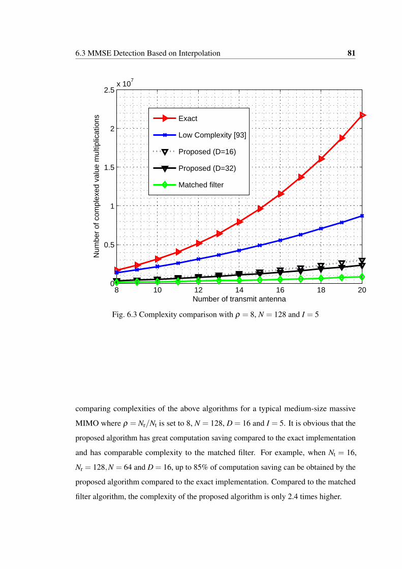
6.3 MMSE Detection Based on Interpolation 81
8 10 12 14 16 18 200
0.5
1
1.5
2
2.5x 10
7
Number of transmit antenna
Num
ber
of c
ompl
exed
val
ue m
ultip
licat
ions
Exact
Low Complexity [93]
Proposed (D=16)
Proposed (D=32)
Matched filter
Fig. 6.3 Complexity comparison with ρ = 8, N = 128 and I = 5
comparing complexities of the above algorithms for a typical medium-size massive
MIMO where ρ = Nr/Nt is set to 8, N = 128, D = 16 and I = 5. It is obvious that the
proposed algorithm has great computation saving compared to the exact implementation
and has comparable complexity to the matched filter. For example, when Nt = 16,
Nr = 128,N = 64 and D = 16, up to 85% of computation saving can be obtained by the
proposed algorithm compared to the exact implementation. Compared to the matched
filter algorithm, the complexity of the proposed algorithm is only 2.4 times higher.

82 A Novel Interpolation Algorithm for Massive MIMO OFDM System Detection
6.4 BER Performance
Based on the profile of channel No.1 in Table 6.1, we firstly generate the time domain
channel coefficients for every path between transmit antennas and receive antennas.
Then FFTs are performed to get the frequency domain channel coefficients. Based
on these coefficients, the frequency domain channel gain matrix of every subcarrier
Hn can be obtained. A rate-1/2, regular (3,6) low-density parity-check (LDPC) code
with codeword length of 10000 bits is employed as the channel code and the maximum
number of iterations of the decoder is 25. The signal modulation of 64-QAM with Gray
mapping is used. For each signal-to-noise (SNR) value, we simulate at least 10000
codewords. In the simulations, there are clipping in soft-output part of the detector (LLR
is constrained to range [−50,50]).
Fig. 6.4 shows the BER performance comparison between the exact MMSE detec-
tion [17], the matched filter, the proposed algorithm with exact Hn (with D = 16,32)
and proposed algorithm with interpolated Hn for non-base subcarriers. The MIMO size
is Nt ×Nr = 16× 128, and the number of subcarrier is set to 256. It is obvious that
the performance of the matched filter algorithm is poor. When computing (5.4) with
proposed algorithm and exact Hn, the BER performance is nearly the same as the exact
one when D = 16, while there is about 0.4dB SNR performance loss when D = 32.
Interpolated Hn in non-base subcarriers also causes some performance loss, e.g. a 0.2dB
performance loss can be observed when using interpolated Hn and Vpn.
6.5 Conclusion
In this chapter, through theoretical analysis and simulations, we found that the matrix
inversion of the Gram matrix G−1n or the regularized Gram matrix (Gn +σ2I)−1 is
strongly correlated between adjacent subcarriers in a massive MIMO-OFDM system.
Then we proposed to use linear interpolation to compute the matrix inversion at non-base
subcarriers. Simulation results showed that the proposed approximation method leads to
marginal performance loss but with considerable complexity saving.

6.5 Conclusion 83
8 8.5 9 9.5 10 10.5 11 11.5 1210
−4
10−3
10−2
10−1
100
SNR (dB)
BE
R
ExactMatche filter
Interp Vnp + exact H
n (D=16)
InterP Vnp +InterP H
n(D=16)
Interp Vnp + exact H
n (D=32)
Fig. 6.4 BER performance comparison for exact MMSE, Matched filter, Proposed Vpn
with exact Hn and Proposed Vpn with interpolated Hn for Nt ×Nr = 16×128 MIMO.


Chapter 7
Summary and Future Work
7.1 Summary
In this thesis, we designed a low complexity channel estimation algorithm for OFDM
systems and various low complexity MIMO detection algorithms. To exploit the correla-
tion between different iterations, an algorithm has been proposed in Chapter 2 to reduce
the matrix inversion from cubic to quadratic level for the second and subsequent itera-
tions. Chapter 3 presents a low complexity PGA algorithm which can deal with channel
spatial correlation effectively. Then a Neumann series expansion based LMMSE channel
estimation algorithm was proposed in Chapter 4 which can reduce the complexity to
O(N logL) where N is the number of subcarriers and L is the number of time domain
channel coefficient taps. In Chapter 5, a Neumann series expansion based LMMSE
algorithm is proposed for massive MIMO uplink detection. With this algorithm, the
total complexity of detecting a length-Nr block is reduced to O(KNtNr) where K is the
number of term in Neumann series expansion and typically it is less than 5. Considering
that the per-tone uplink detection has prohibitive computational complexity in a mas-
sive MIMO-OFDM system, we propose a novel interpolation algorithm to reduce the
complexity of the matrix inversion required by a ZF or MMSE detector in Chapter 61.

86 Summary and Future Work
Compared to the matched filter which has the lower bound complexity, the proposed
algorithm has comparable complexity but has much better BER performance.
7.2 Future Work
7.2.1 Channel estimation for MIMO-OFDM systems
It is most likely that the proposed method in Chapter 4 can be applied to MIMO-OFDM
system and still keep low complexity. Based on the literature survey, a time domain
SAGE algorithm in [99] [100] can reduce the complexity to O(INNtNrL) , where I is
the number of SAGE iterations which is typically less than 4. But as this algorithm
performs channel estimation tap by tap, the estimation latency is huge. By employing
proposed algorithm in a SAGE framework, it is expected that the total complexity can
be reduced to O(INNtNr logL) and the latency can be dramatically reduced because of
employing FFT operation. Specifically, by implementing the single antenna LS channel
estimation ((5) in [99]) with proposed algorithm in Chapter 4, the matrix inversion can
be replaced by L-point input FFT and L-point output IFFT.
7.2.2 Channel estimation for Massive MIMO
The pilot contamination is a key issue for massive MIMO technology [101] [102] [103].
There are two reference papers are closely related to our work. The first one [104]
employs preamble based pilots and uses iterative method to perform data-aided channel
estimation. As virtually, all the data can be assumed as pilots, the effect of pilot contam-
ination can be greatly eliminated. Then the second one [105] employs superimposed
pilots and also performs channel estimation in an iterative manner. The superimposed
pilots can naturally reduce the pilot overhead as all time and frequency resources can
be employed to transmit data. As the length of pilot is of the same length as the data,
it can effectively combat with pilot contamination. When the authors perform channel
1A manuscript based on the main idea of Chapter 6 is being prepared and is planned to be submitted tothe Communication Letter.

7.2 Future Work 87
estimation in [104], they use the approximation of A−1 = diag{A}−1 to perform trivial
matrix inversion which incurs big performance loss as it neglected all non-diagonal
elements. It is hopeful that by employing Neumann series expansion to perform this
matrix inversion, there should be performance gain with small complexity increase.
Similar technique can also be applied to the superimposed pilots case to further reduce
complexity.
7.2.3 Uplink Signal Detection for Massive MIMO-OFDM
In Chapter 6, we have proposed an interpolation based low complexity algorithm for
massive MIMO-OFDM system. But the algorithm can only be applied to conventional
soft-output LMMSE based detector. It cannot be used directly in an IDD system for the
second and subsequent iterations, because the a priori variance is different for different
iteration. From Chapter 2, we know that the matrix inversion between different iterations
are highly correlated and thus can also be interpolated to get low complexity in IDD
system. As a result, a potential future work could be to combine the methods in both
Chapter 2 and Chapter 6 to form a low complexity IDD massive MIMO-OFDM uplink
detector.


Appendix A
Proof of the Equality of Algorithm 1
and Algorithm 2
By using the matrix inversion lemma, Line 4 and 5 in Algorithm 2 can be rewritten to
Vp = V−VHHV−1z HV (A.1)
mp = m−VHHV−1z (y−Hm) (A.2)
where Vz = HVHH +2σ2I. Using hn to denote the nth column of H, we get
vpn = vn − v2
nhHn V−1
z hn (A.3)
mpn = mn − vnhH
n V−1z (y−Hm). (A.4)
Then using Line 7 and Line 8 in Algorithm 2 we have
men =
hHn V−1
z (y−Hm+mnhn)
hHn V−1
z hn(A.5)

90 Proof of the Equality of Algorithm 1 and Algorithm 2
ven =
1hH
n V−1z hn
− vn. (A.6)
Now we will show that hHn V−1
z is a scale version of hHn V−1
n = hHn(2σ2I+HVHH)−1 in
Algorithm 1 (V is the same as V with Vi,i = 1). Obviously, Vn = Vz+(1−vn)hnhHn . By
using the Sherman-Morrison-Woodbury formula of (A+uvH)−1 = A−1 − A−1uvHA−1
1+vHA−1u
we get
hHn V−1
n = hHn V−1
z −hH
n (1− vn)V−1z hnhH
n V−1z
1+(1− vn)hHn V−1
z hn
= hHn V−1
z −(1− vn)(hH
n V−1z hn)(hH
n V−1z )
1+(1− vn)hHn V−1
z hn.
(A.7)
As hHn V−1
z hn is a scalar, (A.7) can be rewritten to
hHn V−1
n =hH
n V−1z
1+(1− vn)hHn V−1
z hn. (A.8)
By noting 11+(1−vn)hH
n V−1z hn
to kn, we get hHn V−1
n = knhHn V−1
z . Then we can represent men
in Algorithm 1 as
men =
xn
µn=
fHn y
fHn hn
=hH
n V−1n (y−hm+mnhn)
hHn V−1
n hn
. (A.9)
In (A.9) by substituting hHn V−1
n with knhHn V−1
z and cancelling the scalar kn, we get the
same result as (A.5).
Now we will show that ven of Algorithm 1 is the same as that in Algorithm 2. From
Line 7 of Algorithm 1, we get
ven =
1fHn hn
−1 =1
hHn V−1
n hn
−1. (A.10)
After substituting (A.8) to (A.10), we get
ven =
1hH
n V−1z
1+(1−vn)hHn V−1
z hnhn
−1 =1
hHn V−1
z hn− vn. (A.11)

91
This is exactly the same as (A.6). Thus, while Algorithm 2 and Algorithm 1 have
different formulae, they actually generate the same extrinsic mean and variance.


Bibliography
[1] Xinyu Gao, Linglong Dai, Yuting Hu, Zhongxu Wang, and Zhaocheng Wang.
Matrix inversion-less signal detection using sor method for uplink large-scale
MIMO systems. In Global Communications Conference (GLOBECOM), 2014
IEEE, pages 3291–3295, 2014.
[2] http://itpp.sourceforge.net/. General specifica-
tion of a time-domain multipath channel. URL
http://itpp.sourceforge.net/4.3.1/classitpp_1_1Channel__Specification.html.
[3] J.H. Winters. On the capacity of radio communication systems with diversity in a
Rayleigh fading environment. IEEE J. Sel. Areas Commun., 5(5):871–878, 1987.
[4] Gerard J Foschini and Michael J Gans. On limits of wireless communications in
a fading environment when using multiple antennas. Wireless personal communi-
cations, 6(3):311–335, 1998.
[5] S. Alamouti. A simple transmit diversity technique for wireless communications.
IEEE J. Sel. Areas Commun., 16(8):1451–1458, 1998.
[6] Gerard J. Foschini. Layered space-time architecture for wireless communication
in a fading environment when using multi-element antennas, 1996. Bell Labs
Technical Journal.
[7] P.W. Wolniansky, G.J. Foschini, G.D. Golden, and R. Valenzuela. V-BLAST: an
architecture for realizing very high data rates over the rich-scattering wireless

94 Bibliography
channel. In Signals, Systems, and Electronics, 1998. ISSSE 98. 1998 URSI
International Symposium on, pages 295–300, 1998.
[8] David Tse and Pramod Viswanath. Fundamentals of wireless communication.
Cambridge university press, 2005.
[9] D. Gesbert, M. Kountouris, R.W. Heath, Chan-Byoung Chae, and T. Salzer.
Shifting the MIMO paradigm. IEEE Signal Process. Mag., 24(5):36–46, 2007.
[10] IEEE LAN/MAN Standards Committee. Overview of 3gpp release 10 v0.0.8.
(2010) online.
[11] IEEE LAN/MAN Standards Committee. System requirements. (2010).
[12] IEEE approved draft standard for it - telecommunications and information ex-
change between systems - LAN/man - specific requirements - part 11: Wireless
LAN medium access control and physical layer specifications - amd 4: En-
hancements for very high throughput for operation in bands below 6GHz. IEEE
P802.11ac/D7.0 September 2013, pages 1–456, December 2013.
[13] J. Hoydis, S. ten Brink, and M. Debbah. Massive MIMO: How many antennas
do we need? In Communication, Control, and Computing (Allerton), 2011 49th
Annual Allerton Conference on, pages 545–550, 2011.
[14] Hoon Huh, G. Caire, H.C. Papadopoulos, and Sean A. Ramprashad. Achieving
large spectral efficiency with tdd and not-so-many base-station antennas. In
Antennas and Propagation in Wireless Communications (APWC), 2011 IEEE-
APS Topical Conference on, pages 1346–1349, 2011.
[15] Hien Quoc Ngo, E.G. Larsson, and T.L. Marzetta. Energy and spectral efficiency
of very large multiuser MIMO systems. IEEE Trans. Commun., 61(4):1436–1449,
2013.
[16] J. Hagenauer, E. Offer, and L. Papke. Iterative decoding of binary block and
convolutional codes. IEEE Trans. Inf. Theory, 42(2):429–445, 1996.

Bibliography 95
[17] Qinghua Guo and D.D. Huang. A concise representation for the soft-in soft-out
lmmse detector. IEEE Commun. Lett., 15(5):566–568, 2011.
[18] M. Tuchler, R. Koetter, and A.C. Singer. Turbo equalization: principles and new
results. IEEE Trans. Commun., 50(5):754–767, 2002.
[19] M. Tuchler, A.C. Singer, and R. Koetter. Minimum mean squared error equal-
ization using a priori information. IEEE Trans. Signal Process., 50(3):673–683,
2002.
[20] Qinghua Guo, Li Ping, and Defeng Huang. A low-complexity iterative channel
estimation and detection technique for doubly selective channels. IEEE Trans.
Wireless Commun., 8(8):4340–4349, 2009.
[21] Joachim Hagenauer. The turbo principle in mobile communications. In Proc.
International Symposium on Nonlinear Theory and its Applications, Xi’an, China,
2002.
[22] Bertrand M Hochwald and Stephan Ten Brink. Achieving near-capacity on a
multiple-antenna channel. Communications, IEEE Transactions on, 51(3):389–
399, 2003.
[23] Simon Haykin, Mathini Sellathurai, Yvo De Jong, and Tricia Willink. Turbo-
mimo for wireless communications. Communications Magazine, IEEE, 42(10):48–
53, 2004.
[24] Y.L.C. de Jong and T.J. Willink. Iterative tree search detection for MIMO wireless
systems. IEEE Trans. Commun., 53(6):930–935, 2005.
[25] R. Koetter, A.C. Singer, and M. Tu{}chler. Turbo equalization. IEEE Signal
Process. Mag., 21(1):67–80, 2004.
[26] Yinsheng Liu, Zhenhui Tan, Hongjie Hu, L.J. Cimini, and G.Y. Li. Channel
estimation for OFDM. IEEE Communications Surveys & Tutorials, 16(4):1891–
1908, 2014.

96 Bibliography
[27] Robert G Gallager. Low-density parity-check codes. Information Theory, IRE
Transactions on, 8(1):21–28, 1962.
[28] R Michael Tanner. A recursive approach to low complexity codes. Information
Theory, IEEE Transactions on, 27(5):533–547, 1981.
[29] David JC MacKay and Radford M Neal. Good codes based on very sparse
matrices. In Cryptography and Coding, pages 100–111. Springer, 1995.
[30] David JC MacKay. Good error-correcting codes based on very sparse matrices.
Information Theory, IEEE Transactions on, 45(2):399–431, 1999.
[31] Noga Alon and Michael Luby. A linear time erasure-resilient code with nearly
optimal recovery. Information Theory, IEEE Transactions on, 42(6):1732–1736,
1996.
[32] IEEE draft standard for information technology–telecommunications and infor-
mation exchange between systems–local and metropolitan area networks–specific
requirements part 11: Wireless LAN medium access control (MAC) and physical
layer (PHY) specifications amendment 5: Enhancements for higher throughput.
IEEE Unapproved Draft Std P802.11n/D9.0 Mar 2009, 2009.
[33] IEEE LAN/MAN Standards Committee et al. Ieee standard for local and
metropolitan area networks part 16: Air interface for fixed broadband wireless
access systems. IEEE Std 802.16TM-2004, 2004.
[34] Yongmin Jung, Chulho Chung, Jaeseok Kim, and Yunho Jung. 7.7Gbps en-
coder design for IEEE 802.11n/ac QC-LDPC codes. In SoC Design Conference
(ISOCC), 2012 International, pages 215–218, November 2012.
[35] A. Mahdi and V. Paliouras. A low complexity-high throughput QC-LDPC encoder.
IEEE Transactions on Signal Processing, 62(10):2696–2708, May 2014.
[36] William E. Ryan. An introduction to ldpc codes. URL
http://www.telecom.tuc.gr/ alex/papers/ryan.pdf.

Bibliography 97
[37] M. Tuchler and A.C. Singer. Turbo equalization: An overview. IEEE Trans. Inf.
Theory, 57(2):920–952, 2011.
[38] A. Tomasoni, M. Ferrari, D. Gatti, F. Osnato, and S. Bellini. A low complexity
turbo MMSE receiver for w-LAN MIMO systems. In Communications, 2006.
ICC ’06. IEEE International Conference on, volume 9, pages 4119–4124, 2006.
[39] Licai Fang, Qinghua Guo, Defeng Huang, and S. Nordholm. A low cost soft map-
per for turbo equalization with high order modulation. In SoC Design Conference
(ISOCC), 2012 International, pages 305–308, 2012.
[40] Qi Wang, Qiuliang Xie, Zhaocheng Wang, Sheng Chen, and L. Hanzo. A universal
low-complexity symbol-to-bit soft demapper. IEEE Transactions on Vehicular
Technology, 63(1):119–130, January 2014.
[41] Patrick Robertson, Emmanuelle Villebrun, and Peter Hoeher. A comparison of
optimal and sub-optimal map decoding algorithms operating in the log domain. In
Communications, 1995. ICC’95 Seattle,’Gateway to Globalization’, 1995 IEEE
International Conference on, volume 2, pages 1009–1013. IEEE, 1995.
[42] E. Agrell, T. Eriksson, A. Vardy, and K. Zeger. Closest point search in lattices.
IEEE Trans. Inf. Theory, 48(8):2201–2214, 2002.
[43] L.G. Barbero and J.S. Thompson. Fixing the complexity of the sphere decoder
for MIMO detection. IEEE Trans. Wireless Commun., 7(6):2131–2142, 2008.
[44] L.G. Barbero and J.S. Thompson. Extending a fixed-complexity sphere decoder
to obtain likelihood information for turbo-MIMO systems. IEEE Trans. Veh.
Technol., 57(5):2804–2814, 2008.
[45] Qinghua Guo, Licai Fang, Defeng Huang, and S. Nordholm. A soft-in soft-out
detection approach using partial Gaussian approximation. In Wireless Communi-
cations & Signal Processing (WCSP), 2012 International Conference on, pages
1–6, 2012.

98 Bibliography
[46] H.-A. Loeliger. An introduction to factor graphs. IEEE Signal Process. Mag.,
21(1):28–41, 2004.
[47] H.-A. Loeliger, J. Dauwels, Junli Hu, S. Korl, Li Ping, and F.R. Kschischang. The
factor graph approach to model-based signal processing. Proc. IEEE, 95(6):1295–
1322, 2007.
[48] P. Som, T. Datta, N. Srinidhi, A. Chockalingam, and B.S. Rajan. Low-complexity
detection in large-dimension MIMO-ISI channels using graphical models. IEEE
J. Sel. Topics Signal Process., 5(8):1497–1511, 2011.
[49] J. Soler-Garrido, R.J. Picchocki, and D. McNamara. Analog MIMO detection
on the basis of belief propagation. In Circuits and Systems, 2006. MWSCAS ’06.
49th IEEE International Midwest Symposium on, volume 2, pages 50–54, 2006.
[50] Xiumei Yang, Yong Xiong, and Fan Wang. An adaptive MIMO system based on
unified belief propagation detection. In Communications, 2007. ICC ’07. IEEE
International Conference on, pages 4156–4161, 2007.
[51] M. Suneel, P. Som, A. Chockalingam, and B.S. Rajan. Belief propagation based
decoding of large non-orthogonal STBCs. In Information Theory, 2009. ISIT
2009. IEEE International Symposium on, pages 2003–2007, 2009.
[52] P. Som, T. Datta, A. Chockalingam, and B.S. Rajan. Improved large-MIMO
detection based on damped belief propagation. In Information Theory (ITW 2010,
Cairo), 2010 IEEE Information Theory Workshop on, pages 1–5, 2010.
[53] Yong Soo Cho, Jaekwon Kim, Won Young Yang, and Chung G Kang. MIMO-
OFDM wireless communications with MATLAB. John Wiley & Sons, 2010.
[54] F. Rusek, D. Persson, Buon Kiong Lau, E.G. Larsson, T.L. Marzetta, O. Edfors,
and F. Tufvesson. Scaling up MIMO: Opportunities and challenges with very
large arrays. IEEE Signal Process. Mag., 30(1):40–60, 2013.

Bibliography 99
[55] E.G. Larsson. MIMO detection methods: How they work [lecture notes]. IEEE
Signal Process. Mag., 26(3):91–95, 2009.
[56] Xiaodong Wang and H.V. Poor. Iterative (turbo) soft interference cancellation
and decoding for coded CDMA. IEEE Trans. Commun., 47(7):1046–1061, 1999.
[57] M. Witzke, S. Baro, F. Schreckenbach, and J. Hagenauer. Iterative detection of
MIMO signals with linear detectors. In Signals, Systems and Computers, 2002.
Conference Record of the Thirty-Sixth Asilomar Conference on, volume 1, pages
289–293, 2002.
[58] D.N. Liu and M.P. Fitz. Low complexity affine MMSE detector for iterative
detection-decoding MIMO OFDM systems. IEEE Trans. Commun., 56(1):150–
158, 2008.
[59] Seunghwan Choi, Jongkyung Kim, and Jong-Soo Seo. A simplified MMSE
detection for iterative receivers in multiple antenna systems. In Broadband Multi-
media Systems and Broadcasting (BMSB), 2011 IEEE International Symposium
on, pages 1–5, 2011.
[60] C. Studer, S. Fateh, and D. Seethaler. ASIC implementation of soft-input soft-
output MIMO detection using MMSE parallel interference cancellation. IEEE J.
Solid-State Circuits, 46(7):1754–1765, 2011.
[61] J.-J. van de Beek, O. Edfors, M. Sandell, S.K. Wilson, and P. Ola Borjesson. On
channel estimation in OFDM systems. In Vehicular Technology Conference, 1995
IEEE 45th, volume 2, pages 815–819, 1995.
[62] Koichi Ishihara, Kazuaki Takeda, and Fumiyuki Adachi. Iterative channel estima-
tion for frequency-domain equalization of dsss signals. IEICE transactions on
communications, 90(5):1171–1180, 2007.

100 Bibliography
[63] Chan-Tong Lam, D.D. Falconer, and F. Danilo-Lemoine. Iterative frequency
domain channel estimation for dft-precoded ofdm systems using in-band pilots.
IEEE J. Sel. Areas Commun., 26(2):348–358, 2008.
[64] Nian Geng, Xiaojun Yuan, and Li Ping. Dual-diagonal lmmse channel estimation
for OFDM systems. IEEE Trans. Signal Process., 60(9):4734–4746, 2012.
[65] Yongzhe Xie and C. N. Georghiades. Two em-type channel estimation algorithms
for OFDM with transmitter diversity. IEEE Transactions on Communications,
51(1):106–115, January 2003.
[66] K. Vardhan, S.K. Mohammed, A. Chockalingam, and B.S. Rajan. A low-
complexity detector for large MIMO systems and multicarrier CDMA systems.
IEEE J. Sel. Areas Commun., 26(3):473–485, 2008.
[67] N. Srinidhi, T. Datta, A. Chockalingam, and B.S. Rajan. Layered tabu search
algorithm for large-MIMO detection and a lower bound on ML performance.
IEEE Trans. Commun., 59(11):2955–2963, 2011.
[68] B.S. Rajan, S.K. Mohammed, A. Chockalingam, and N. Srinidhi. Low-complexity
near-ML decoding of large non-orthogonal STBCs using reactive tabu search. In
Information Theory, 2009. ISIT 2009. IEEE International Symposium on, pages
1993–1997, 2009.
[69] M. Wu, C. Dick, J.R. Cavallaro, and C. Studer. Iterative detection and decoding
in 3GPP LTE-based massive MIMO systems. In Signal Processing Conference
(EUSIPCO), 2014 Proceedings of the 22nd European, pages 96–100, 2014.
[70] M. Wu, Bei Yin, A. Vosoughi, C. Studer, J.R. Cavallaro, and C. Dick. Approxi-
mate matrix inversion for high-throughput data detection in the large-scale MIMO
uplink. In Circuits and Systems (ISCAS), 2013 IEEE International Symposium
on, pages 2155–2158, 2013.

Bibliography 101
[71] Bei Yin, M. Wu, C. Studer, J.R. Cavallaro, and C. Dick. Implementation trade-offs
for linear detection in large-scale MIMO systems. In Acoustics, Speech and Signal
Processing (ICASSP), 2013 IEEE International Conference on, pages 2679–2683,
2013.
[72] M. Wu, Bei Yin, Guohui Wang, C. Dick, J.R. Cavallaro, and C. Studer. Large-
scale MIMO detection for 3GPP LTE: Algorithms and FPGA implementations.
IEEE J. Sel. Topics Signal Process., 8(5):916–929, 2014.
[73] S. Ohno, S. Munesada, and E. Manasseh. Low-complexity approximate lmmse
channel estimation for OFDM systems. In Signal & Information Processing
Association Annual Summit and Conference (APSIPA ASC), 2012 Asia-Pacific,
pages 1–4, 2012.
[74] Pierluigi Salvo Rossi, Ralf R MüLler, and Ove Edfors. Linear mmse estimation
of time–frequency variant channels for mimo-ofdm systems. Signal Processing,
91(5):1157–1167, 2011.
[75] F. Pena-Campos, R. Carrasco-Alvarez, O. Longoria-Gandara, and R. Parra-
Michel. Estimation of fast time-varying channels in OFDM systems using
two-dimensional prolate. IEEE Trans. Wireless Commun., 12(2):898–907, 2013.
[76] P. Hammarberg, F. Rusek, and O. Edfors. Channel estimation algorithms for
OFDM-idma: Complexity and performance. IEEE Trans. Wireless Commun.,
11(5):1722–1732, 2012.
[77] D. Auras, R. Leupers, and G.H. Ascheid. A novel reduced-complexity soft-input
soft-output MMSE MIMO detector: Algorithm and efficient VLSI architecture.
In Communications (ICC), 2014 IEEE International Conference on, pages 4722–
4728, 2014.
[78] P. Suthisopapan, K. Kasai, A. Meesomboon, and V. Imtawil. Achieving near
capacity of non-binary LDPC coded large MIMO systems with a novel ultra low-

102 Bibliography
complexity soft-output detector. IEEE Trans. Wireless Commun., 12(10):5185–
5199, 2013.
[79] Yuan Yang and Hai-lin Zhang. A simplified mmse-based iterative receiver for
mimo systems. Journal of Zhejiang University SCIENCE A, 10(10):1389–1394,
2009.
[80] A. Krishnamoorthy and D. Menon. Matrix inversion using cholesky decom-
position. In Signal Processing: Algorithms, Architectures, Arrangements, and
Applications (SPA), 2013, pages 70–72, 2013.
[81] M. Senst and G. Ascheid. How the framework of expectation propagation yields
an iterative IC-lmmse MIMO receiver. In Global Telecommunications Conference
(GLOBECOM 2011), 2011 IEEE, pages 1–6, 2011.
[82] J. Vogt and A. Finger. Improving the max-log-MAP turbo decoder. Electronics
Letters, 36(23):1937–1939, 2000.
[83] Claus-Peter Schnorr and Martin Euchner. Lattice basis reduction: improved prac-
tical algorithms and solving subset sum problems. Mathematical programming,
66(1-3):181–199, 1994.
[84] Christoph Buchheim, Alberto Caprara, and Andrea Lodi. An effective branch-
and-bound algorithm for convex quadratic integer programming. Mathematical
programming, 135(1-2):369–395, 2012.
[85] George Tsoulos. MIMO system technology for wireless communications. CRC
press, 2006.
[86] Young-Jin Kim and Gi-Hong Im. Pilot-symbol assisted power delay profile
estimation for MIMO-OFDM systems. IEEE Commun. Lett., 16(1):68–71, 2012.
[87] M Kay Steven. Fundamentals of statistical signal processing. PTR Prentice-Hall,
Englewood Cliffs, NJ, 1993.

Bibliography 103
[88] GW Stewart. Matrix algorithms: Basic decompositions (volume 1). Society for
Industrial and Applied Math, 1998.
[89] H.V. Sorensen and C.S. Burrus. Efficient computation of the DFT with only a
subset of input or output points. IEEE Trans. Signal Process., 41(3):1184–1200,
1993.
[90] Henrik Asplund, Andrés Alayón Glazunov, Andreas F Molisch, Klaus I Pedersen,
and Martin Steinbauer. The cost 259 directional channel model-part ii: macrocells.
Wireless Communications, IEEE Transactions on, 5(12):3434–3450, 2006.
[91] William C Jakes and Donald C Cox. Microwave mobile communications. Wiley-
IEEE Press, 1994.
[92] Liang Lin, Niu Kai, Xu Wenjun, Tian Baoyu, Gong Ping, and Sun Shaohui.
Channel estimate with PDP assumption and interference RS knowledge in LTE
system. In Communication Technology (ICCT), 2012 IEEE 14th International
Conference on, pages 496–500, 2012.
[93] M. Borgmann and H. Bolcskei. Interpolation-based efficient matrix inversion for
MIMO-OFDM receivers. In Signals, Systems and Computers, 2004. Conference
Record of the Thirty-Eighth Asilomar Conference on, volume 2, pages 1941–1947,
2004.
[94] Andreas Burg, Helmut Bölcskei, Moritz Borgmann, Davide Cescato, and Jan
Hansen. Method for calculating functions of the channel matrices in linear
mimo-ofdm data transmission, June 22 2010. US Patent 7,742,536.
[95] Jian A. Zhang, Xiaojing Huang, Hajime Suzuki, and Zhuo Chen. Gaussian
approximation based interpolation for channel matrix inversion in MIMO-OFDM
systems. IEEE Trans. Wireless Commun., 12(3):1407–1417, 2013.

104 Bibliography
[96] A. Salari, S.M. Fakhraie, and A. Abbasfar. Algorithm and FPGA implementation
of interpolation-based soft output mmse mimo detector for 3GPP LTE. IET
Communications, 8(4):492–499, 2014.
[97] Jihoon Choi and R.W. Heath. Interpolation based transmit beamforming for
MIMO-OFDM with limited feedback. IEEE Trans. Signal Process., 53(11):4125–
4135, 2005.
[98] L. Fang, L. Xu, and D. Huang. Low complexity iterative MMSE-PIC detection
for medium-size massive MIMO. IEEE Wireless Communications Letters, to be
published. Early Access.
[99] J. Ylioinas, M.R. Raghavendra, and M. Juntti. Avoiding matrix inversion in dd
sage channel estimation in MIMO-OFDM with m-QAM. In Vehicular Technology
Conference Fall (VTC 2009-Fall), 2009 IEEE 70th, pages 1–5, 2009.
[100] J. Ylioinas and M. Juntti. Iterative joint detection, decoding, and channel estima-
tion in turbo-coded MIMO-OFDM. IEEE Trans. Veh. Technol., 58(4):1784–1796,
2009.
[101] J. Jose, A. Ashikhmin, T.L. Marzetta, and S. Vishwanath. Pilot contamination and
precoding in multi-cell tdd systems. IEEE Trans. Wireless Commun., 10(8):2640–
2651, 2011.
[102] B. Gopalakrishnan and N. Jindal. An analysis of pilot contamination on multi-user
MIMO cellular systems with many antennas. In Signal Processing Advances in
Wireless Communications (SPAWC), 2011 IEEE 12th International Workshop on,
pages 381–385, 2011.
[103] N. Krishnan, R.D. Yates, and N.B. Mandayam. Cellular systems with many
antennas: Large system analysis under pilot contamination. In Communication,
Control, and Computing (Allerton), 2012 50th Annual Allerton Conference on,
pages 1220–1224, 2012.

Bibliography 105
[104] Junjie Ma and Li Ping. Data-aided channel estimation in large antenna systems.
IEEE Trans. Signal Process., 62(12):3111–3124, 2014.
[105] Han Zhang, Shan Gao, Dong Li, Hongbin Chen, and Liang Yang. On superim-
posed pilot for channel estimation in multi-cell multiuser mimo uplink: large
system analysis. 2015.


![Reduced minimax state estimation · 2016. 12. 28. · Vivien Mallet, Sergiy Zhuk. Reduced minimax state estimation. [Research Report] ... L’archive ouverte pluridisciplinaire HAL,](https://img.pdfslide.us/doc/110x75/61428e04d9e4dc11f47f2006/reduced-minimax-state-estimation-2016-12-28-vivien-mallet-sergiy-zhuk-reduced.jpg)