REDD QGIS workshop - Using RADAR imagery to map Forests

The purpose of this practical is to introduce the process of using L-band RADAR imagery to

map changes in carbon stocks in Miombo Woodland. It centres on an area from Southern

Malawi as a case study.

Specifically we will be looking at abrupt/severe biomass loss events between 2007 and 2010.

Within this practical we use the following definitions:

- Forested Land: Land with Biomass > 10tC/ha

- Abrupt/severe forest loss events: Land that was forested in 2007 but that has lost at

least 50% of its biomass between 2007 and 2010.

If performing this process in the future for your organisation, it is important to:

a) Carefully define forest (in terms of biomass) for the particular country/project.

b) Understand what extent of biomass change is of interest (e.g. a loss of 50% or a loss

of 10%?)

By default, due to the image processing required, this practical will also introduce:

- Working with Raster datasets in QGIS (importing and setting their properties)

- Merging geographically adjacent Raster datasets using QGIS’ GDAL plugin

- Using QGIS’ Raster Calculator to create new Raster datasets

- Reclassifying Raster Datasets

- Exploring Raster values within pre-defined areas (i.e. polygon features) using QGIS’

Zonal Statistics plugin

It assumes a basic knowledge of RADAR theory, how RADAR is used to identify types of

land cover & land cover change, how terrain influences the returned signal…and

consequently, why we need to correct RADAR imagery produced for the impact of terrain.

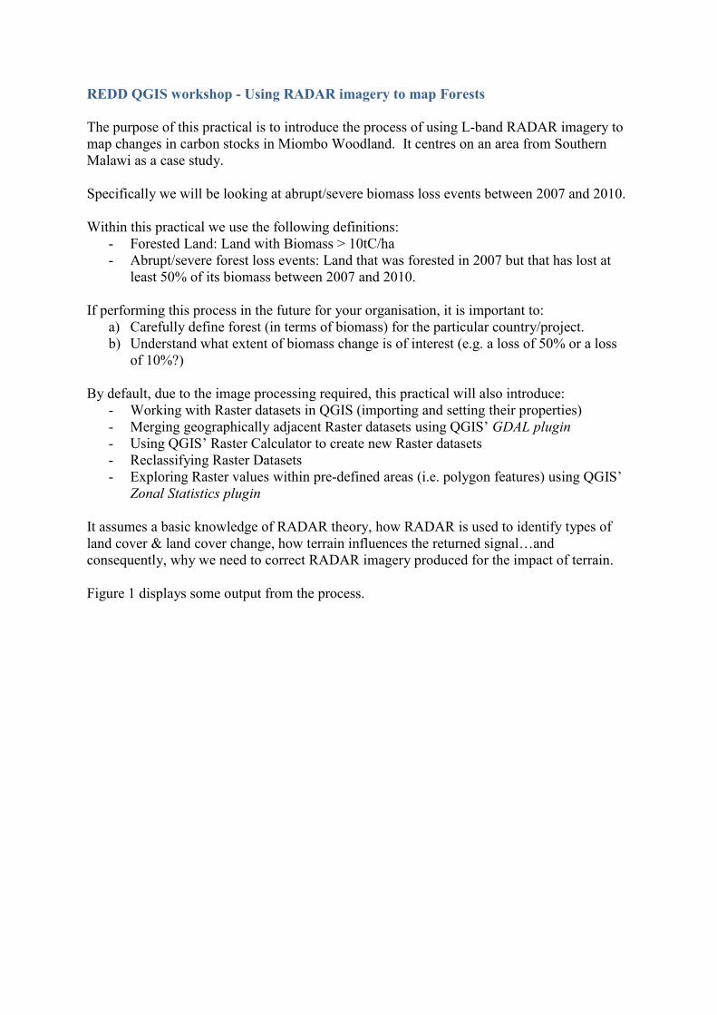
Figure 1 displays some output from the process.

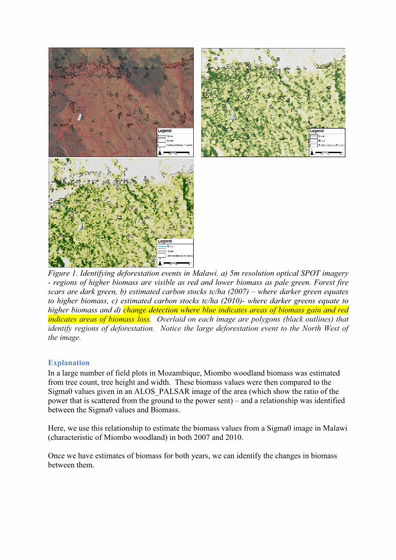
Figure 1. Identifying deforestation events in Malawi. a) 5m resolution optical SPOT imagery

- regions of higher biomass are visible as red and lower biomass as pale green. Forest fire

scars are dark green, b) estimated carbon stocks tc/ha (2007) – where darker green equates

to higher biomass, c) estimated carbon stocks tc/ha (2010)- where darker greens equate to

higher biomass and d) change detection where blue indicates areas of biomass gain and red

indicates areas of biomass loss. Overlaid on each image are polygons (black outlines) that

identify regions of deforestation. Notice the large deforestation event to the North West of

the image.

Explanation

In a large number of field plots in Mozambique, Miombo woodland biomass was estimated

from tree count, tree height and width. These biomass values were then compared to the

Sigma0 values given in an ALOS_PALSAR image of the area (which show the ratio of the

power that is scattered from the ground to the power sent) – and a relationship was identified

between the Sigma0 values and Biomass.

Here, we use this relationship to estimate the biomass values from a Sigma0 image in Malawi

(characteristic of Miombo woodland) in both 2007 and 2010.

Once we have estimates of biomass for both years, we can identify the changes in biomass

between them.

The Process

Figure 2 below outlines the processing-chain that is used to create the biomass maps and

change maps. Take time to familiarise yourself with each stage of the process and ask

questions if you are unsure of any stage.

Figure 2: Flow chart to summarise the components of the image processing chain used to

identify areas of deforestation. The configuration file holds information about which settings

should be applied in MapReady.

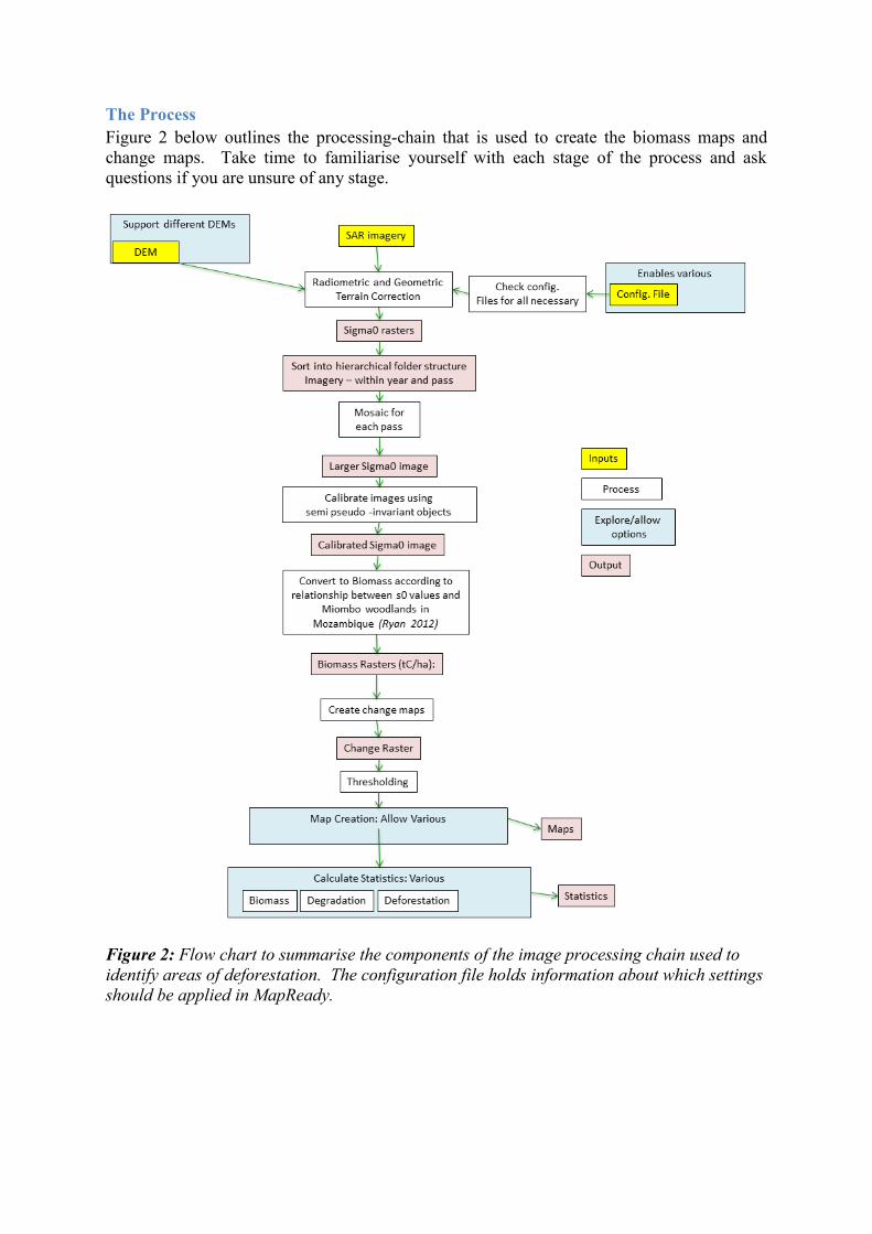
Worked Example

Area of Interest

The satellite scene used in this case study lies to the West of Blantyre City, covering the

Mwanza district entirely, and parts of the Blantyre, Chikwawa and Ntcheu districts.

Figure 3. Study Area: The extent of the study area (red) on a base map of Malawi, its

districts (yellow), primary roads (black) and cities (black)

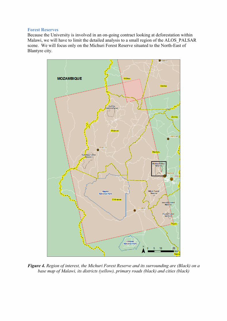
Forest Reserves

Because the University is involved in an on-going contract looking at deforestation within

Malawi, we will have to limit the detailed analysis to a small region of the ALOS_PALSAR

scene. We will focus only on the Michuri Forest Reserve situated to the North-East of

Blantyre city.

Figure 4. Region of interest, the Michuri Forest Reserve and its surrounding are (Black) on a

base map of Malawi, its districts (yellow), primary roads (black) and cities (black)

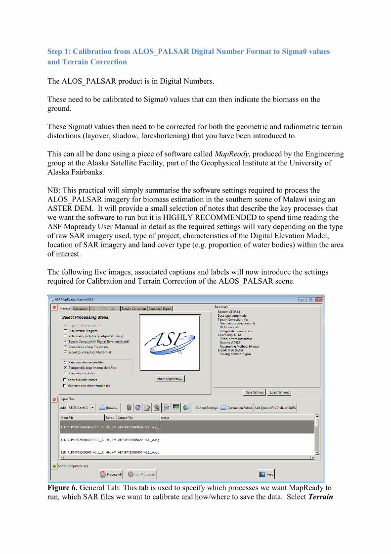
Step 1: Calibration from ALOS_PALSAR Digital Number Format to Sigma0 values

and Terrain Correction

The ALOS_PALSAR product is in Digital Numbers.

These need to be calibrated to Sigma0 values that can then indicate the biomass on the

ground.

These Sigma0 values then need to be corrected for both the geometric and radiometric terrain

distortions (layover, shadow, foreshortening) that you have been introduced to.

This can all be done using a piece of software called MapReady, produced by the Engineering

group at the Alaska Satellite Facility, part of the Geophysical Institute at the University of

Alaska Fairbanks.

NB: This practical will simply summarise the software settings required to process the

ALOS_PALSAR imagery for biomass estimation in the southern scene of Malawi using an

ASTER DEM. It will provide a small selection of notes that describe the key processes that

we want the software to run but it is HIGHLY RECOMMENDED to spend time reading the

ASF Mapready User Manual in detail as the required settings will vary depending on the type

of raw SAR imagery used, type of project, characteristics of the Digital Elevation Model,

location of SAR imagery and land cover type (e.g. proportion of water bodies) within the area

of interest.

The following five images, associated captions and labels will now introduce the settings

required for Calibration and Terrain Correction of the ALOS_PALSAR scene.

Figure 6. General Tab: This tab is used to specify which processes we want MapReady to

run, which SAR files we want to calibrate and how/where to save the data. Select Terrain

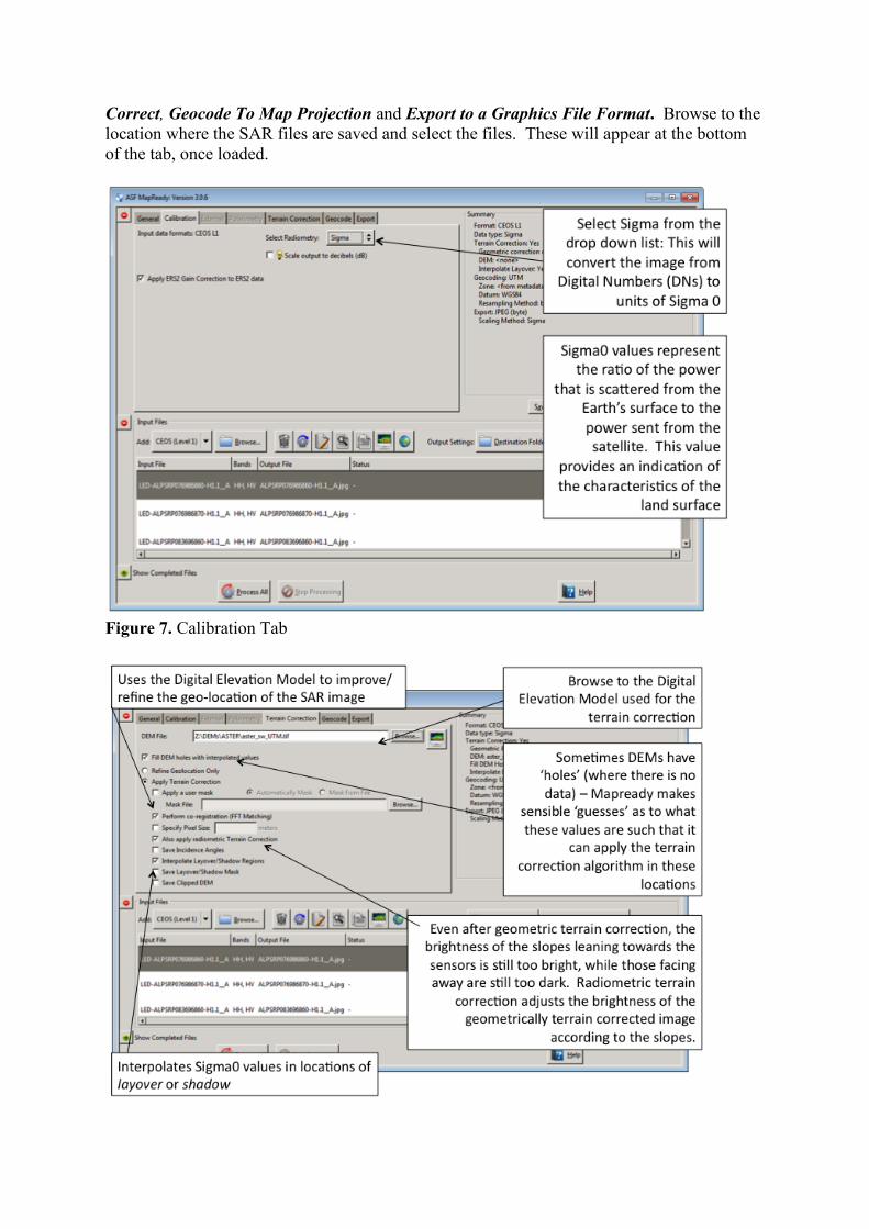
Correct, Geocode To Map Projection and Export to a Graphics File Format. Browse to the

location where the SAR files are saved and select the files. These will appear at the bottom

of the tab, once loaded.

Figure 7. Calibration Tab

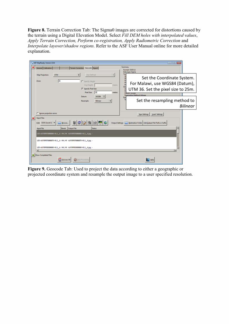
Figure 8. Terrain Correction Tab: The Sigma0 images are corrected for distortions caused by

the terrain using a Digital Elevation Model. Select Fill DEM holes with interpolated values,

Apply Terrain Correction, Perform co-registration, Apply Radiometric Correction and

Interpolate layover/shadow regions. Refer to the ASF User Manual online for more detailed

explanation.

Figure 9. Geocode Tab: Used to project the data according to either a geographic or

projected coordinate system and resample the output image to a user specified resolution.

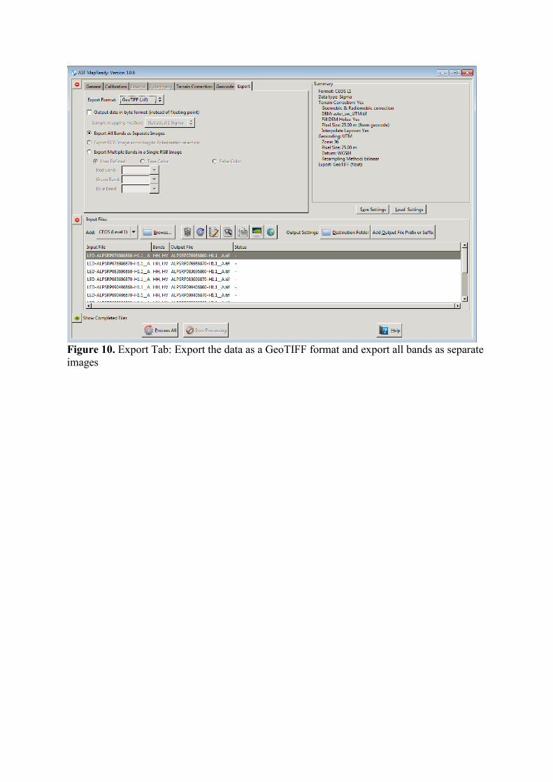
Figure 10. Export Tab: Export the data as a GeoTIFF format and export all bands as separate

images

The Sigma0 images are separated in the Data Folder according to the year that they were

taken, and the time of year they were taken (the ‘pass’). To begin, we need to merge the

Sigma0 images from each pass. We will first import the images from each pass, and then

merge them. Only import and merge images from one pass at a time or you it will become

confusing which images belong to which pass and QGIS will slow down.

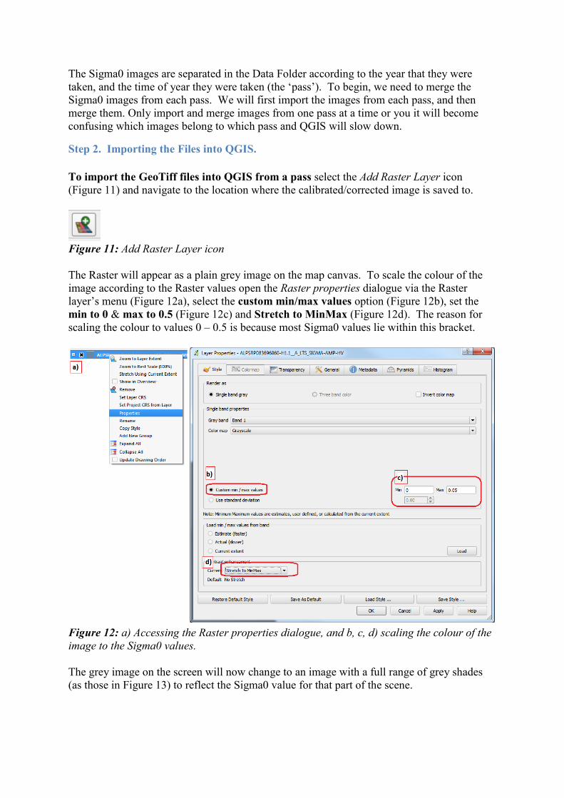
Step 2. Importing the Files into QGIS.

To import the GeoTiff files into QGIS from a pass select the Add Raster Layer icon

(Figure 11) and navigate to the location where the calibrated/corrected image is saved to.

Figure 11: Add Raster Layer icon

The Raster will appear as a plain grey image on the map canvas. To scale the colour of the

image according to the Raster values open the Raster properties dialogue via the Raster

layer’s menu (Figure 12a), select the custom min/max values option (Figure 12b), set the

min to 0 & max to 0.5 (Figure 12c) and Stretch to MinMax (Figure 12d). The reason for

scaling the colour to values 0 – 0.5 is because most Sigma0 values lie within this bracket.

Figure 12: a) Accessing the Raster properties dialogue, and b, c, d) scaling the colour of the

image to the Sigma0 values.

The grey image on the screen will now change to an image with a full range of grey shades

(as those in Figure 13) to reflect the Sigma0 value for that part of the scene.

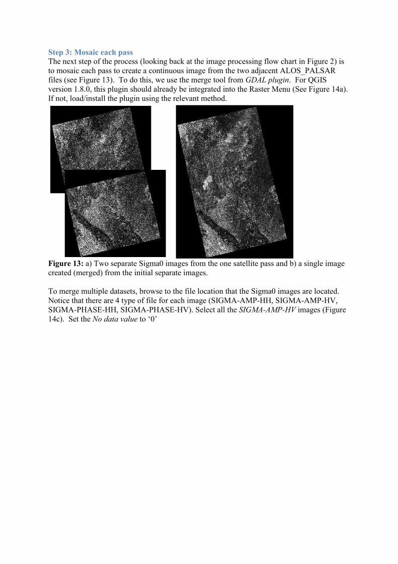
Step 3: Mosaic each pass

The next step of the process (looking back at the image processing flow chart in Figure 2) is

to mosaic each pass to create a continuous image from the two adjacent ALOS_PALSAR

files (see Figure 13). To do this, we use the merge tool from GDAL plugin. For QGIS

version 1.8.0, this plugin should already be integrated into the Raster Menu (See Figure 14a).

If not, load/install the plugin using the relevant method.

Figure 13: a) Two separate Sigma0 images from the one satellite pass and b) a single image

created (merged) from the initial separate images.

To merge multiple datasets, browse to the file location that the Sigma0 images are located.

Notice that there are 4 type of file for each image (SIGMA-AMP-HH, SIGMA-AMP-HV,

SIGMA-PHASE-HH, SIGMA-PHASE-HV). Select all the SIGMA-AMP-HV images (Figure

14c). Set the No data value to ‘0’

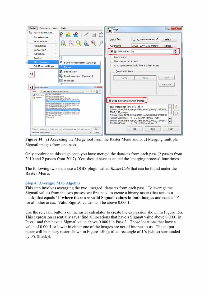
Figure 14. a) Accessing the Merge tool from the Raster Menu and b, c) Merging multiple

Sigma0 images from one pass.

Only continue to this stage once you have merged the datasets from each pass (2 passes from

2010 and 2 passes from 2007). You should have executed the ‘merging process’ four times.

The following two steps use a QGIS plugin called RasterCalc that can be found under the

Raster Menu.

Step 4: Average: Map Algebra

This step involves averaging the two ‘merged’ datasets from each pass. To average the

Sigma0 values from the two passes, we first need to create a binary raster (that acts as a

mask) that equals ‘1’ where there are valid Sigma0 values in both images and equals ‘0’

for all other areas. Valid Sigma0 values will be above 0.0001.

Use the relevant buttons on the raster calculator to create the expression shown in Figure 15a.

This expression essentially says ‘find all locations that have a Sigma0 value above 0.0001 in

Pass 1 and that have a Sigma0 value above 0.0001 in Pass 2’. Those locations that have a

value of 0.0001 or lower in either one of the images are not of interest to us. The output

raster will be binary raster shown in Figure 15b (a tilted rectangle of 1’s (white) surrounded

by 0’s (black)).

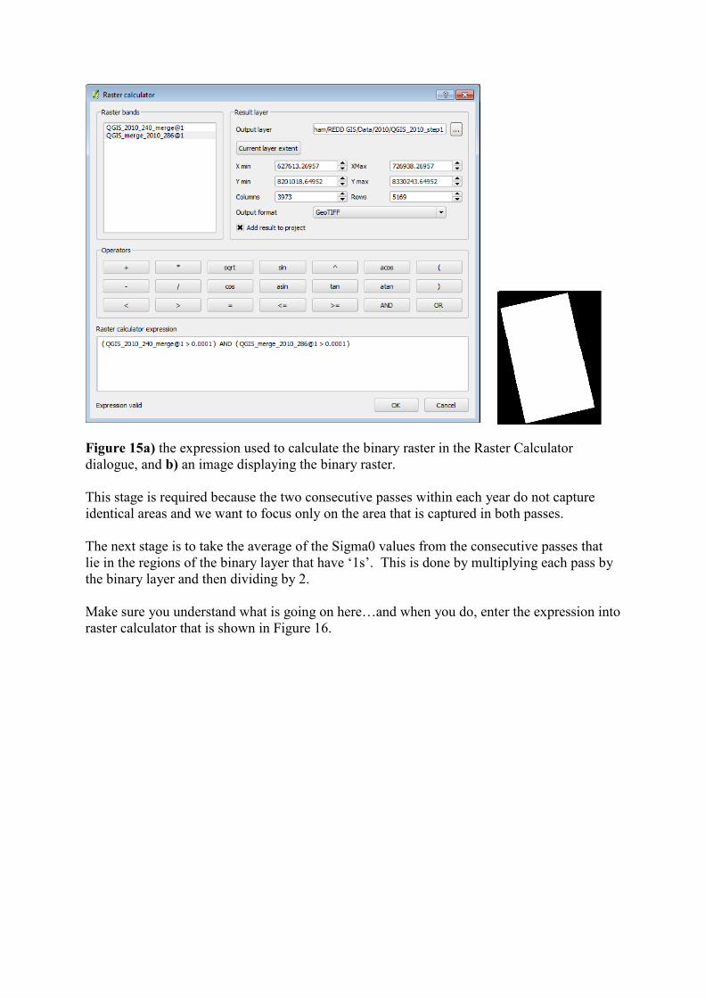
Figure 15a) the expression used to calculate the binary raster in the Raster Calculator

dialogue, and b) an image displaying the binary raster.

This stage is required because the two consecutive passes within each year do not capture

identical areas and we want to focus only on the area that is captured in both passes.

The next stage is to take the average of the Sigma0 values from the consecutive passes that

lie in the regions of the binary layer that have ‘1s’. This is done by multiplying each pass by

the binary layer and then dividing by 2.

Make sure you understand what is going on here…and when you do, enter the expression into

raster calculator that is shown in Figure 16.

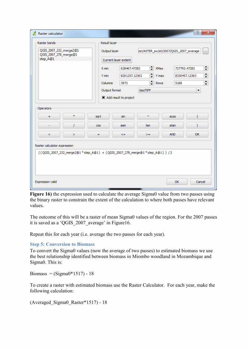
Figure 16) the expression used to calculate the average Sigma0 value from two passes using

the binary raster to constrain the extent of the calculation to where both passes have relevant

values.

The outcome of this will be a raster of mean Sigma0 values of the region. For the 2007 passes

it is saved as a ‘QGIS_2007_average’ in Figure16.

Repeat this for each year (i.e. average the two passes for each year).

Step 5: Conversion to Biomass

To convert the Sigma0 values (now the average of two passes) to estimated biomass we use

the best relationship identified between biomass in Miombo woodland in Mozambique and

Sigma0. This is:

Biomass = (Sigma0*1517) - 18

To create a raster with estimated biomass use the Raster Calculator. For each year, make the

following calculation:

(Averaged_Sigma0_Raster*1517) - 18

Step 6: Creating a change map

Now that we have a Raster of estimated biomass in 2007 and another for 2010, we want to

understand how much change there has been in the three year period between. To do this, we

divide the 2010 Biomass Map by the 2007 Biomass Map. This will create a Raster of values

that span between 0 and 2. Cells that have a value near 1 have not changed much between

2007 and 2010 (neither a loss nor gain in Biomass). Cells that have a value between 1 and 2

have gained biomass between 2007 and 2010. Cells that have a value between 0 and 1 have

lost biomass between 2007 and 2010.

Calculate the change map using the raster calculator. Within the expression box enter:

Biomass_Raster_2010/Biomass_Raster_2007