Embed Size (px)
Citation preview
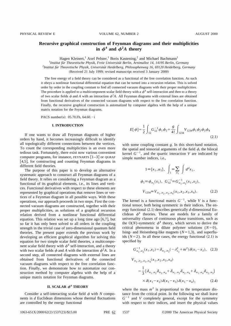
Recursive graphical construction of Feynman diagrams and their multiplicitiesin f4 and f2A theory
Hagen Kleinert,1 Axel Pelster,1 Boris Kastening,2 and Michael Bachmann1
1Institut fur Theoretische Physik, Freie Universitat Berlin, Arnimallee 14, 14195 Berlin, Germany2Institut fur Theoretische Physik, Universitat Heidelberg, Philosophenweg 16, 69120 Heidelberg, Germany
~Received 21 July 1999; revised manuscript received 3 January 2000!
The free energy of a field theory can be considered as a functional of the free correlation function. As suchit obeys a nonlinear functional differential equation that can be turned into a recursion relation. This is solvedorder by order in the coupling constant to find all connected vacuum diagrams with their proper multiplicities.The procedure is applied to a multicomponent scalar field theory with a f4 self-interaction and then to a theoryof two scalar fields f and A with an interaction f2A . All Feynman diagrams with external lines are obtainedfrom functional derivatives of the connected vacuum diagrams with respect to the free correlation function.Finally, the recursive graphical construction is automatized by computer algebra with the help of a uniquematrix notation for the Feynman diagrams.
PACS number~s!: 05.70.Fh, 64.60.2i
I. INTRODUCTION
If one wants to draw all Feynman diagrams of higherorders by hand, it becomes increasingly difficult to identifyall topologically different connections between the vertices.To count the corresponding multiplicities is an even moretedious task. Fortunately, there exist now various convenientcomputer programs, for instance, FEYNARTS @1–3# or QGRAF
@4,5#, for constructing and counting Feynman diagrams indifferent field theories.
The purpose of this paper is to develop an alternativesystematic approach to construct all Feynman diagrams of afield theory. It relies on considering a Feynman diagram as afunctional of its graphical elements, i.e., its lines and verti-ces. Functional derivatives with respect to these elements arerepresented by graphical operations that remove lines or ver-tices of a Feynman diagram in all possible ways. With theseoperations, our approach proceeds in two steps. First the con-nected vacuum diagrams are constructed, together with theirproper multiplicities, as solutions of a graphical recursionrelation derived from a nonlinear functional differentialequation. This relation was set up a long time ago @6,7#, butso far it has only been solved to all orders in the couplingstrength in the trivial case of zero-dimensional quantum fieldtheories. The present paper extends the previous work bydeveloping an efficient graphical algorithm for solving thisequation for two simple scalar field theories, a multicompo-nent scalar field theory with f4 self-interaction, and a theorywith two scalar fields f and A with the interaction f2A . In asecond step, all connected diagrams with external lines areobtained from functional derivatives of the connectedvacuum diagrams with respect to the free correlation func-tion. Finally, we demonstrate how to automatize our con-struction method by computer algebra with the help of aunique matrix notation for Feynman diagrams.
II. SCALAR f4 THEORY
Consider a self-interacting scalar field f with N compo-nents in d Euclidean dimensions whose thermal fluctuationsare controlled by the energy functional
E@f#5
1
2 E12G12
21f1f21
g
4! E1234V1234f1f2f3f4
~2.1!
with some coupling constant g. In this short-hand notation,the spatial and tensorial arguments of the field f, the bilocalkernel G21, and the quartic interaction V are indicated bysimple number indices, i.e.,
1[$x1 ,a1%, E1[(
a1
E ddx1 ,
f1[fa1~x1!, G12
21[Ga1 ,a2
21 ~x1 ,x2!,
V1234[Va1 ,a2 ,a3 ,a4~x1 ,x2 ,x3 ,x4!. ~2.2!
The kernel is a functional matrix G21, while V is a func-tional tensor, both being symmetric in their indices. The en-ergy functional ~2.1! describes generically d-dimensional Eu-clidean f4 theories. These are models for a family ofuniversality classes of continuous phase transitions, such asthe O(N)-symmetric f4 theory, which serves to derive thecritical phenomena in dilute polymer solutions (N50),Ising- and Heisenberg-like magnets (N51,3), and superflu-ids (N52). In all these cases, the energy functional ~2.1! isspecified by
Ga1 ,a2
21 ~x1 ,x2!5da1 ,a2~2]x1
21m2!d~x12x2!, ~2.3!
Va1 ,a2 ,a3 ,a4~x1 ,x2 ,x3 ,x4!
5
1
3$da1 ,a2
da3 ,a41da1 ,a3
da2 ,a41da1 ,a4
da2 ,a3%
3d~x12x2!d~x12x3!d~x12x4!, ~2.4!
where the mass m2 is proportional to the temperature dis-tance from the critical point. In the following we shall leaveG21 and V completely general, except for the symmetrywith respect to their indices, and insert the physical values
PHYSICAL REVIEW E AUGUST 2000VOLUME 62, NUMBER 2
PRE 621063-651X/2000/62~2!/1537~23!/$15.00 1537 ©2000 The American Physical Society
~2.3! and ~2.4! at the end. By using natural units in which theBoltzmann constant kB times the temperature T equals unity,the partition function is determined as a functional integralover the Boltzmann weight e2E@f#
Z5E Df e2E@f# ~2.5!
and may be evaluated perturbatively as a power series in thecoupling constant g. From this we obtain the negative freeenergy W5ln Z as an expansion
W5 (p50
`1
p! S 2g
4! D p
W ~p !. ~2.6!
The coefficients W (p) may be displayed as connectedvacuum diagrams constructed from lines and vertices. Eachline represents a free correlation function
~2.7!
which is the functional inverse of the kernel G21 in theenergy functional ~2.1!, defined by
E2G12G23
215d13 . ~2.8!
The vertices represent an integral over the interaction
~2.9!
To construct all connected vacuum diagrams contributing toW (p) to each order p in perturbation theory, one connects pvertices with 4p legs in all possible ways according to Fey-nman’s rules, which follow from Wick’s expansion of corre-lation functions into a sum of all pair contractions. Thisyields an increasing number of Feynman diagrams, each witha certain multiplicity that follows from combinatorics. In to-tal there are 4!pp! ways of ordering the 4p legs of the pvertices. This number is reduced by permutations of the legsand the vertices that leave a vacuum diagram invariant. De-noting the number of self-, double, triple, and fourfold con-nections with S, D, T, F, there are 2!S, 2!D, 3!T, 4!F legpermutations. An additional reduction arises from the num-ber N of vertex permutations, leaving the vacuum diagramsunchanged, where the vertices remain attached to the linesemerging from them in the same way as before. The result-ing multiplicity of a connected vacuum diagram in the f4
theory is therefore given by the formula @9,10#
M f4E50
5
4!pp!
2!S1D3!T4!FN. ~2.10!
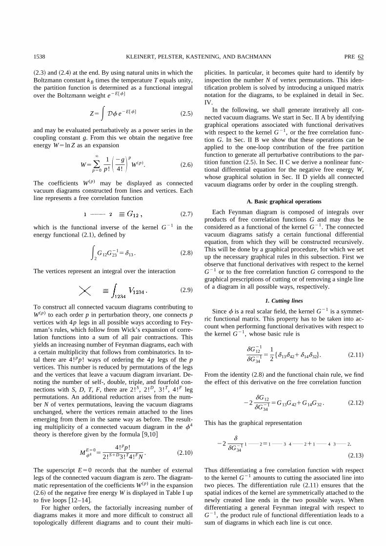
The superscript E50 records that the number of externallegs of the connected vacuum diagram is zero. The diagram-matic representation of the coefficients W (p) in the expansion~2.6! of the negative free energy W is displayed in Table I upto five loops @12–14#.
For higher orders, the factorially increasing number ofdiagrams makes it more and more difficult to construct alltopologically different diagrams and to count their multi-
plicities. In particular, it becomes quite hard to identify byinspection the number N of vertex permutations. This iden-tification problem is solved by introducing a uniqued matrixnotation for the diagrams, to be explained in detail in Sec.IV.
In the following, we shall generate iteratively all con-nected vacuum diagrams. We start in Sec. II A by identifyinggraphical operations associated with functional derivativeswith respect to the kernel G21, or the free correlation func-tion G. In Sec. II B we show that these operations can beapplied to the one-loop contribution of the free partitionfunction to generate all perturbative contributions to the par-tition function ~2.5!. In Sec. II C we derive a nonlinear func-tional differential equation for the negative free energy W,whose graphical solution in Sec. II D yields all connectedvacuum diagrams order by order in the coupling strength.
A. Basic graphical operations
Each Feynman diagram is composed of integrals overproducts of free correlation functions G and may thus beconsidered as a functional of the kernel G21. The connectedvacuum diagrams satisfy a certain functional differentialequation, from which they will be constructed recursively.This will be done by a graphical procedure, for which we setup the necessary graphical rules in this subsection. First weobserve that functional derivatives with respect to the kernelG21 or to the free correlation function G correspond to thegraphical prescriptions of cutting or of removing a single lineof a diagram in all possible ways, respectively.
1. Cutting lines
Since f is a real scalar field, the kernel G21 is a symmet-ric functional matrix. This property has to be taken into ac-count when performing functional derivatives with respect tothe kernel G21, whose basic rule is
dG1221
dG3421 5
1
2$d13d421d14d32%. ~2.11!
From the identity ~2.8! and the functional chain rule, we findthe effect of this derivative on the free correlation function
22dG12
dG3421 5G13G421G14G32 . ~2.12!
This has the graphical representation
22d
dG3421 1 251 3 4 211 4 3 2.
~2.13!
Thus differentiating a free correlation function with respectto the kernel G21 amounts to cutting the associated line intotwo pieces. The differentiation rule ~2.11! ensures that thespatial indices of the kernel are symmetrically attached to thenewly created line ends in the two possible ways. Whendifferentiating a general Feynman integral with respect toG21, the product rule of functional differentiation leads to asum of diagrams in which each line is cut once.
1538 PRE 62KLEINERT, PELSTER, KASTENING, AND BACHMANN
With this graphical operation, the product of two fieldscan be rewritten as a derivative of the energy functional withrespect to the kernel
f1f252dE@f#
dG1221 , ~2.14!
as follows directly from ~2.1! and ~2.11!. Applying the sub-stitution rule ~2.14! to the functional integral for the fullyinteracting two-point function
G1251
Z E Df f1f2e2E@f#, ~2.15!
we obtain the fundamental identity
G12522dW
dG1221 . ~2.16!
Thus, by cutting a line of the connected vacuum diagrams inall possible ways, we obtain all diagrams of the fully inter-acting two-point function. Analytically this has a Taylor se-ries expansion in powers of the coupling constant g similarto ~2.6!
G125 (p50
`1
p! S 2g
4! D p
G12~p ! ~2.17!
with coefficients
G12~p !
522dW ~p !
dG1221 . ~2.18!
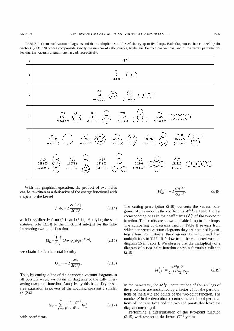
The cutting prescription ~2.18! converts the vacuum dia-grams of pth order in the coefficients W (p) in Table I to thecorresponding ones in the coefficients G12
(p) of the two-pointfunction. The results are shown in Table II up to four loops.The numbering of diagrams used in Table II reveals fromwhich connected vacuum diagrams they are obtained by cut-ting a line. For instance, the diagrams 15.1–15.5 and theirmultiplicities in Table II follow from the connected vacuumdiagram 15 in Table I. We observe that the multiplicity of adiagram of a two-point function obeys a formula similar to~2.10!:
M f4E52
5
4!pp!2!
2!S1D3!TN. ~2.19!
In the numerator, the 4!pp! permutations of the 4p legs ofthe p vertices are multiplied by a factor 2! for the permuta-tions of the E52 end points of the two-point function. Thenumber N in the denominator counts the combined permuta-tions of the p vertices and the two end points that leave thediagram unchanged.
Performing a differentiation of the two-point function~2.15! with respect to the kernel G21 yields
TABLE I. Connected vacuum diagrams and their multiplicities of the f4 theory up to five loops. Each diagram is characterized by thevector ~S,D,T,F;N! whose components specify the number of self-, double, triple, and fourfold connections, and of the vertex permutationsleaving the vacuum diagram unchanged, respectively.
PRE 62 1539RECURSIVE GRAPHICAL CONSTRUCTION OF FEYNMAN . . .
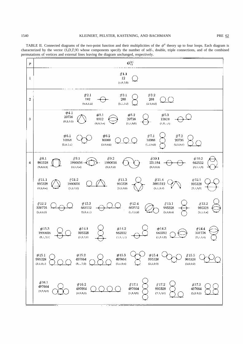
TABLE II. Connected diagrams of the two-point function and their multiplicities of the f4 theory up to four loops. Each diagram ischaracterized by the vector ~S,D,T;N! whose components specify the number of self-, double, triple connections, and of the combinedpermutations of vertices and external lines leaving the diagram unchanged, respectively.
1540 PRE 62KLEINERT, PELSTER, KASTENING, AND BACHMANN

22dG12
dG3421 5G12342G12G34 , ~2.20!
where G1234 denotes the fully interacting four-point function
G123451
Z E Df f1f2f3f4e2E@f#. ~2.21!
The term G12G34 in ~2.20! subtracts a certain set of discon-nected diagrams from G1234 . By subtracting all disconnecteddiagrams from G1234 , we obtain the connected four-pointfunction
G1234c [G12342G12G342G13G242G14G23 ~2.22!
in the form
G1234c
522dG12
dG3421 2G13G242G14G23 . ~2.23!
The first term contains all diagrams obtained by cutting aline in the diagrams of the two-point function G12 . The sec-ond and third terms remove from these the disconnected dia-grams. In this way we obtain the perturbative expansion
G1234c
5 (p51
`1
p! S 2g
4! D p
G1234c ,~p ! ~2.24!
with coefficients
G1234c ,~p !
522dG12
~p !
dG3421 2 (
q50
p S pq D ~G13
~p2q !G24~q !
1G14~p2q !G23
~q !!.
~2.25!
They are listed diagrammatically in Table III up to threeloops. As before in Table II, the multiple numbering in TableIII indicates the origin of each diagram of the connectedfour-point function. For instance, the diagram 11.2.2, 11.4.3,14.1.2, 14.3.3 in Table III stems together with its multiplicityfrom the diagrams 11.2, 11.4, 14.1, 14.3 in Table II.
The multiplicity of each diagram of a connected four-point function obeys a formula similar to ~2.19!:
M f4E54
5
4!pp!4!
2!S1D3!TN. ~2.26!
This multiplicity decomposes into equal parts if the spatialindices 1, 2, 3, 4 are assigned to the E54 end points of theconnected four-point function, for instance:
~2.27!
Generalizing the multiplicities ~2.10!, ~2.19!, and ~2.26! forconnected vacuum diagrams, two- and four-point functionsto an arbitrary connected correlation function with an evennumber E of end points, we see that
M f4E
5
4!pp!E!
2!S1D3!T4!FN, ~2.28!
where N counts the number of combined permutations ofvertices and external lines which leave the diagram un-changed.
2. Removing lines
We now study the graphical effect of functional deriva-tives with respect to the free correlation function G, wherethe basic differentiation rule ~2.11! becomes
dG12
dG345
1
2$d13d421d14d32%. ~2.29!
We represent this graphically by extending the elements ofFeynman diagrams by an open dot with two labeled line endsrepresenting the delta function:
1 –+– 25d12 ~2.30!
Thus we can write the differentiation ~2.29! graphically asfollows:
d
d3 41 25
1
2$1 –+– 3 4 –+– 211 –+– 4 3 –+– 2%. ~2.31!
Differentiating a line with respect to the free correlationfunction removes the line, leaving in a symmetrized way thespatial indices of the free correlation function on the verticesto which the line was connected.
The effect of this derivative is illustrated by studying thediagrammatic effect of the operator
L5E12
G12
d
dG12. ~2.32!
Applying L to a connected vacuum diagram in W (p), thefunctional derivative d/dG12 generates diagrams in each ofwhich one of the 2p lines of the original vacuum diagram isremoved. Subsequently, the removed lines are again rein-serted, so that the connected vacuum diagrams W (p) areeigenfunctions of L , whose eigenvalues 2p count the lines ofthe diagrams:
LW ~p !52pW ~p !. ~2.33!
PRE 62 1541RECURSIVE GRAPHICAL CONSTRUCTION OF FEYNMAN . . .
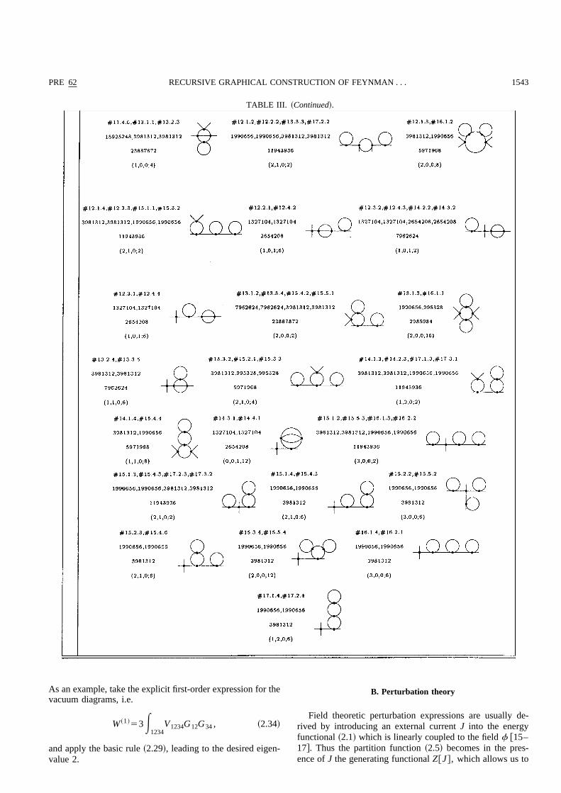
TABLE III. Connected diagrams of the four-point function and their multiplicities of the f4 theory up to three loops. Each diagram ischaracterized by the vector ~S, D, T; N! whose components specify the number of self-, double, triple connections, and of the combinedpermutations of vertices and external lines leaving the diagram unchanged, respectively.
1542 PRE 62KLEINERT, PELSTER, KASTENING, AND BACHMANN
As an example, take the explicit first-order expression for thevacuum diagrams, i.e.
W ~1 !53E
1234V1234G12G34 , ~2.34!
and apply the basic rule ~2.29!, leading to the desired eigen-value 2.
B. Perturbation theory
Field theoretic perturbation expressions are usually de-rived by introducing an external current J into the energyfunctional ~2.1! which is linearly coupled to the field f @15–17#. Thus the partition function ~2.5! becomes in the pres-ence of J the generating functional Z@J# , which allows us to
TABLE III. ~Continued!.
PRE 62 1543RECURSIVE GRAPHICAL CONSTRUCTION OF FEYNMAN . . .
find all free n-point functions from functional derivativeswith respect to this external current J. In the normal phase ofa f4 theory, the expectation value of the field f is zero andonly correlation functions of an even number of fields arenonzero. To calculate all of these, it is possible to substitutetwo functional derivatives with respect to the current J byone functional derivative with respect to the kernel G21.This reduces the number of functional derivatives in eachorder of perturbation theory by one-half and has the addi-tional advantage that the introduction of the current J be-comes superfluous.
1. Current approach
Recall briefly the standard perturbative treatment, inwhich the energy functional ~2.1! is artificially extended by asource term
E@f ,J#5E@f#2E1J1f1 . ~2.35!
The functional integral for the generating functional
Z@J#5E Df e2E@f ,J# ~2.36!
is first explicitly calculated for a vanishing coupling constantg, yielding
Z ~0 !@J#5expH 2
1
2Tr ln G21
1
1
2 E12G12 J1J2J ,
~2.37!
where the trace of the logarithm of the kernel is defined bythe series ~see p. 16 in Ref. @18#!
Tr ln G215 (
n51
`~21 !n11
n E1...n
$G1221
2d12%¯$Gn121
2dn1%.
~2.38!
If the coupling constant g does not vanish, one expands thegenerating functional Z@J# in powers of the quartic interac-tion V , and reexpresses the resulting powers of the fieldwithin the functional integral ~2.36! as functional derivativeswith respect to the current J. The original partition function~2.5! can thus be obtained from the free generating func-tional ~2.37! by the formula
Z5expH 2
g
4! E1234V1234
d4
dJ1dJ2dJ3dJ4J Z ~0 !@J#U
J50
.
~2.39!
Expanding the exponential in a power series, we arrive at theperturbation expansion
Z5H 11
2g
4! E1234
V1234
d4
dJ1dJ2dJ3dJ4
1
1
2 S 2g
4! D 2E12345678
V1234V5678
3
d8
dJ1dJ2dJ3dJ4dJ5dJ6dJ7dJ81 . . .J Z ~0 !@J#U
J50
,
~2.40!
in which the pth order contribution for the partition functionrequires the evaluation of 4p functional derivatives with re-spect to the current J.
2. Kernel approach
The derivation of the perturbation expansion simplifies, ifwe use functional derivatives with respect to the kernel G21
in the energy functional ~2.1! rather than with respect to thecurrent J. This allows us to substitute the previous expres-sion ~2.39! for the partition function by
Z5expH 2
g
6 E1234V1234
d2
dG1221dG34
21J eW~0 !, ~2.41!
where the zeroth order of the negative free energy has thediagrammatic representation
~2.42!
Expanding again the exponential in a power series, we obtain
Z5H 11
2g
6 E1234
V1234
d2
dG1221dG34
21
1
1
2 S 2g
6 D 2E12345678
V1234V5678
3
d4
dG1221dG34
21dG5621dG78
21 1 . . .J eW~0 !. ~2.43!
Thus we need only half as many functional derivatives thanin ~2.40!. Taking into account ~2.11!, ~2.12!, and ~2.38!, weobtain
dW ~0 !
dG1221 52
1
2G12 ,
d2W ~0 !
dG1221dG34
21 5
1
4$G13G241G14G23%,
~2.44!
such that the partition function Z becomes
Z5H 11
2g
4!3E
1234V1234G12G341
1
2 S 2g
4! D 2
3E12345678
V1234V5678 @9G12G34G56G78
124G15G26G37G48172G12G35G46G78#1 . . .J eW~0 !.
~2.45!
This has the diagrammatic representation
1544 PRE 62KLEINERT, PELSTER, KASTENING, AND BACHMANN
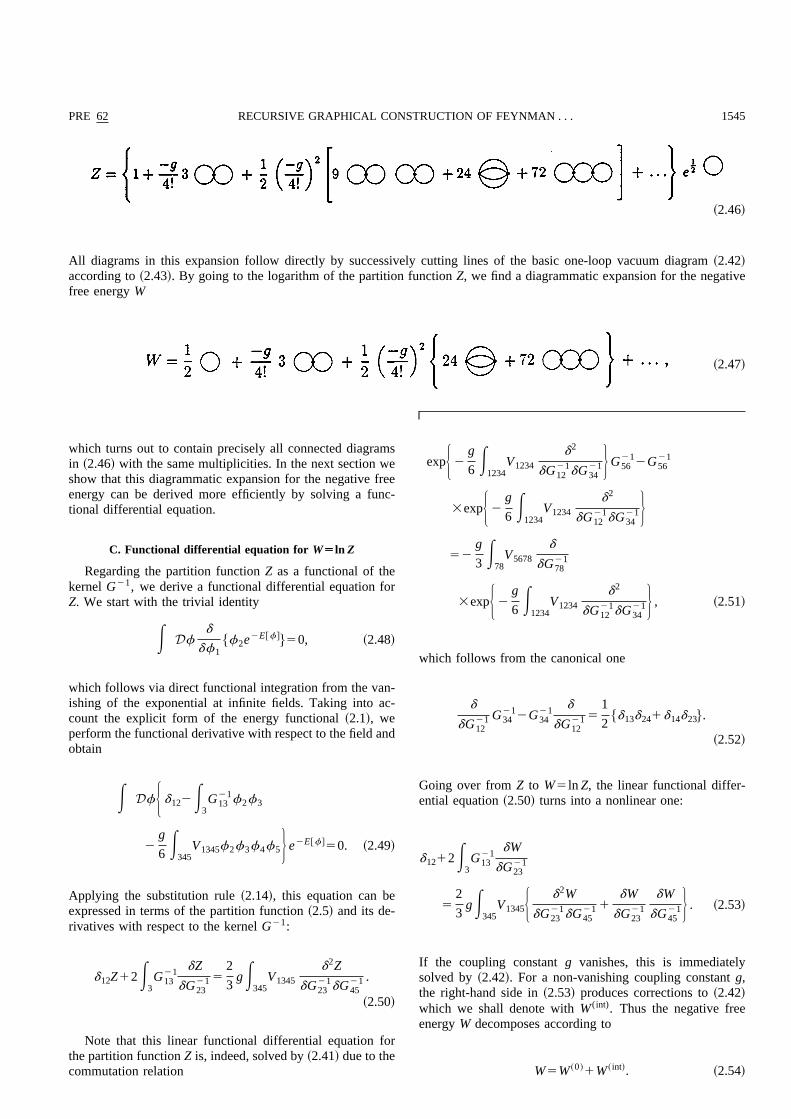
~2.46!
All diagrams in this expansion follow directly by successively cutting lines of the basic one-loop vacuum diagram ~2.42!according to ~2.43!. By going to the logarithm of the partition function Z, we find a diagrammatic expansion for the negativefree energy W
~2.47!
which turns out to contain precisely all connected diagramsin ~2.46! with the same multiplicities. In the next section weshow that this diagrammatic expansion for the negative freeenergy can be derived more efficiently by solving a func-tional differential equation.
C. Functional differential equation for WÄln Z
Regarding the partition function Z as a functional of thekernel G21, we derive a functional differential equation forZ. We start with the trivial identity
E Dfd
df1$f2e2E@f#%50, ~2.48!
which follows via direct functional integration from the van-ishing of the exponential at infinite fields. Taking into ac-count the explicit form of the energy functional ~2.1!, weperform the functional derivative with respect to the field andobtain
E DfH d122E3G13
21f2f3
2
g
6 E345V1345f2f3f4f5J e2E@f#
50. ~2.49!
Applying the substitution rule ~2.14!, this equation can beexpressed in terms of the partition function ~2.5! and its de-rivatives with respect to the kernel G21:
d12Z12E3G13
21 dZ
dG2321 5
2
3gE
345V1345
d2Z
dG2321dG45
21 .
~2.50!
Note that this linear functional differential equation forthe partition function Z is, indeed, solved by ~2.41! due to thecommutation relation
expH 2
g
6 E1234V1234
d2
dG1221dG34
21J G5621
2G5621
3expH 2
g
6 E1234V1234
d2
dG1221dG34
21J52
g
3 E78V5678
d
dG7821
3expH 2
g
6 E1234V1234
d2
dG1221dG34
21J , ~2.51!
which follows from the canonical one
d
dG1221 G34
212G34
21 d
dG1221 5
1
2$d13d241d14d23%.
~2.52!
Going over from Z to W5ln Z, the linear functional differ-ential equation ~2.50! turns into a nonlinear one:
d1212E3G13
21 dW
dG2321
5
2
3gE
345V1345H d2W
dG2321dG45
21 1
dW
dG2321
dW
dG4521J . ~2.53!
If the coupling constant g vanishes, this is immediatelysolved by ~2.42!. For a non-vanishing coupling constant g,the right-hand side in ~2.53! produces corrections to ~2.42!which we shall denote with W (int). Thus the negative freeenergy W decomposes according to
W5W ~0 !1W ~ int!. ~2.54!
PRE 62 1545RECURSIVE GRAPHICAL CONSTRUCTION OF FEYNMAN . . .
Inserting this into ~2.53! and taking into account ~2.44!, weobtain the following functional differential equation for theinteraction negative free energy W (int):
E12
G1221 dW ~ int!
dG1221
5
g
4 E1234V1234G12G342
g
3 E1234V1234G12
dW ~ int!
dG3421
1
g
3 E1234V1234H d2W ~ int!
dG1221dG34
21 1
dW ~ int!
dG1221
dW ~ int!
dG3421 J .
~2.55!
With the help of the functional chain rule, the first and sec-ond derivatives with respect to the kernel G21 are rewrittenas
d
dG1221 52E
34G13G24
d
dG34~2.56!
and
d2
dG1221dG34
21 5E5678
G15G26G37G48
d2
dG56dG78
1
1
2 E56$G13G25G461G14G25G36
1G23G15G461G24G15G36%d
dG56,
~2.57!
respectively, so that the functional differential equation~2.55! for W (int) takes the form ~compare Eq. ~51! in Ref. @7#!
E12
G12
dW ~ int!
dG1252
g
4 E1234V1234G12G34
2gE123456
V1234G12G35G46
dW ~ int!
dG56
2
g
3 E12345678V1234G15G26G37G48
3H d2W ~ int!
dG56dG781
dW ~ int!
dG56
dW ~ int!
dG78J .
~2.58!
D. Recursion relation and graphical solution
We now convert the functional differential equation~2.58! into a recursion relation by expanding W (int) into apower series in g:
W ~ int!5 (
p51
`1
p! S 2g
4! D p
W ~p !. ~2.59!
Using the property ~2.33! that the coefficient W (p) satisfiesthe eigenvalue problem of the line numbering operator~2.32!, we obtain the recursion relation
W ~p11 !512E
123456V1234G12G35G46
dW ~p !
dG56
14E12345678
V1234G15G26G37G48
d2W ~p !
dG56dG78
14 (q51
p21 S pq D E
12345678V1234G15G26G37G48
3
dW ~p2q !
dG56
dW ~q !
dG78~2.60!
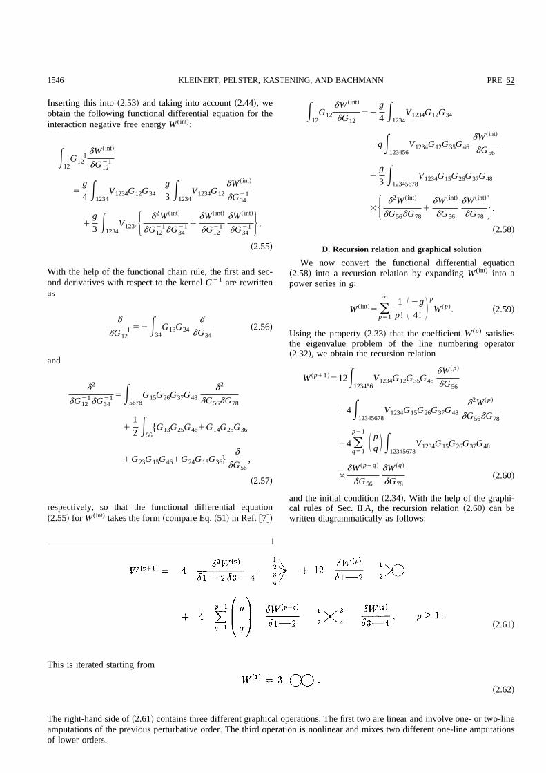
and the initial condition ~2.34!. With the help of the graphi-cal rules of Sec. II A, the recursion relation ~2.60! can bewritten diagrammatically as follows:
~2.61!
This is iterated starting from
~2.62!
The right-hand side of ~2.61! contains three different graphical operations. The first two are linear and involve one- or two-lineamputations of the previous perturbative order. The third operation is nonlinear and mixes two different one-line amputationsof lower orders.
1546 PRE 62KLEINERT, PELSTER, KASTENING, AND BACHMANN
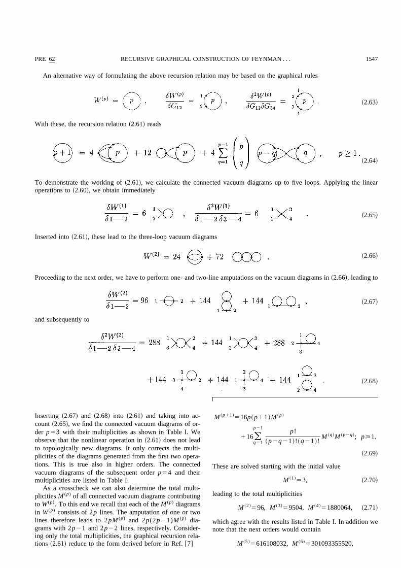
An alternative way of formulating the above recursion relation may be based on the graphical rules
~2.63!
With these, the recursion relation ~2.61! reads
~2.64!
To demonstrate the working of ~2.61!, we calculate the connected vacuum diagrams up to five loops. Applying the linearoperations to ~2.60!, we obtain immediately
~2.65!
Inserted into ~2.61!, these lead to the three-loop vacuum diagrams
~2.66!
Proceeding to the next order, we have to perform one- and two-line amputations on the vacuum diagrams in ~2.66!, leading to
~2.67!
and subsequently to
~2.68!
Inserting ~2.67! and ~2.68! into ~2.61! and taking into ac-count ~2.65!, we find the connected vacuum diagrams of or-der p53 with their multiplicities as shown in Table I. Weobserve that the nonlinear operation in ~2.61! does not leadto topologically new diagrams. It only corrects the multi-plicities of the diagrams generated from the first two opera-tions. This is true also in higher orders. The connectedvacuum diagrams of the subsequent order p54 and theirmultiplicities are listed in Table I.
As a crosscheck we can also determine the total multi-plicities M (p) of all connected vacuum diagrams contributingto W (p). To this end we recall that each of the M (p) diagramsin W (p) consists of 2p lines. The amputation of one or twolines therefore leads to 2pM (p) and 2p(2p21)M (p) dia-grams with 2p21 and 2p22 lines, respectively. Consider-ing only the total multiplicities, the graphical recursion rela-tions ~2.61! reduce to the form derived before in Ref. @7#
M ~p11 !516p~p11 !M ~p !
116(q51
p21p!
~p2q21 !!~q21 !!M ~q !M ~p2q !; p>1.
~2.69!
These are solved starting with the initial value
M ~1 !53, ~2.70!
leading to the total multiplicities
M ~2 !596, M ~3 !
59504, M ~4 !51880064, ~2.71!
which agree with the results listed in Table I. In addition wenote that the next orders would contain
M ~5 !5616108032, M ~6 !
5301093355520,
PRE 62 1547RECURSIVE GRAPHICAL CONSTRUCTION OF FEYNMAN . . .
M ~7 !5205062331760640 ~2.72!
connected vacuum diagrams.
III. SCALAR f2A THEORY
For the sake of generality, let us also study the situationwhere the quartic interaction of the f4 theory is generated bya scalar field A from a cubic f2 A interaction. The associatedenergy functional
E@f ,A#5E ~0 !@f ,A#1E ~ int!@f ,A# ~3.1!
decomposes into the free part
E ~0 !@f ,A#5
1
2 E12G12
21f1f21
1
2 E12H12
21A1A2 ~3.2!
and the interaction
E ~ int!@f ,A#5
Ag
2 E123
V123f1f2A3 . ~3.3!
Indeed, as the field A appears only quadratically in ~3.1!, thefunctional integral for the partition function
Z5E DfDAe2E@f ,A# ~3.4!
can be exactly evaluated with respect to the field A, yielding
Z5E Df e2E~eff!@f# ~3.5!
with the effective energy functional
E ~eff!@f#52
1
2Tr ln H21
1
1
2 E12G12
21f1f2
2
g
8 E123456V125V346H56f1f2f3f4 . ~3.6!
Apart from a trivial shift due to the negative free energy ofthe field A, the effective energy functional ~3.6! coincideswith that of a f4 theory in Eq. ~2.1! with the quartic inter-action
V1234523E56
V125V346H56 . ~3.7!
If we supplement the previous Feynman rules ~2.7!, ~2.9! bythe free correlation function of the field A
~3.8!
and the cubic interaction
~3.9!
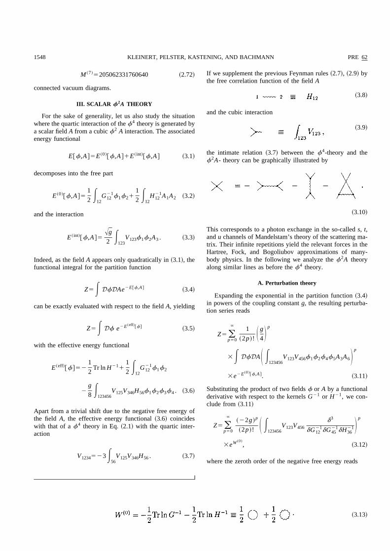
the intimate relation ~3.7! between the f4-theory and thef2A- theory can be graphically illustrated by
~3.10!
This corresponds to a photon exchange in the so-called s, t,and u channels of Mandelstam’s theory of the scattering ma-trix. Their infinite repetitions yield the relevant forces in theHartree, Fock, and Bogoliubov approximations of many-body physics. In the following we analyze the f2A theoryalong similar lines as before the f4 theory.
A. Perturbation theory
Expanding the exponential in the partition function ~3.4!in powers of the coupling constant g, the resulting perturba-tion series reads
Z5 (p50
`1
~2p !! S g
4 D p
3E DfDAS E123456
V123V456f1f2f4f5A3A6D p
3e2E~0 !@f ,A#. ~3.11!
Substituting the product of two fields f or A by a functionalderivative with respect to the kernels G21 or H21, we con-clude from ~3.11!
Z5 (p50
`~22g !p
~2p !! S E123456
V123V456
d3
dG1221dG45
21dH3621D p
3eW~0 !, ~3.12!
where the zeroth order of the negative free energy reads
~3.13!
1548 PRE 62KLEINERT, PELSTER, KASTENING, AND BACHMANN
Inserting ~3.13! in ~3.12!, the first-order contribution to thenegative free energy yields
W ~1 !52E
123456V123V456H36G14G25
1E123456
V123V456H36G12G45 , ~3.14!
which corresponds to the Feynman diagrams
~3.15!
B. Functional differential equation for WÄln Z
The derivation of a functional differential equation for thenegative free energy W requires the combination of two in-dependent steps. Consider first the identity
E DfDAd
df1$f2e2E@f ,A#%50, ~3.16!
which immediately yields with the energy functional ~3.1!
d12Z12E3G13
21 dZ
dG2321 12AgE
34V134
d $^A4&Z%
dG2321 50,
~3.17!
where ^A& denotes the expectation value of the field A. Inorder to close the functional differential equation, we con-sider the second identity
E DfDAd
dA1e2E@f ,A#
50, ~3.18!
which leads to
^A1&Z5AgE234
V234H14
dZ
dG2321 . ~3.19!
Inserting ~3.19! in ~3.17!, we result in the desired functionaldifferential equation for the negative free energy W5ln Z:
d1212E2G13
21 dW
dG2321 522gE
34567V134V567
3H47H d2W
dG2321dG56
21 1
dW
dG2321
dW
dG5621J .
~3.20!
A subsequent separation ~2.54! of the zeroth-order ~3.13!leads to a functional differential equation for the interactionpart of the free energy W (int):
E12
G1221 dW ~ int!
dG1221 52
g
4 E123456V123V456H36
3$G12G4512G14G25%
1gE123456
V123V456G12H36
dW ~ int!
dG4521
2gE123456
V123V456H36H d2W ~ int!
dG1221dG45
21
1
dW ~ int!
dG1221
dW ~ int!
dG4521 J . ~3.21!
Taking into account the functional chain rules ~2.56!, ~2.57!,the functional derivatives with respect to G21 in ~3.21! canbe rewritten in terms of G:
E12
G12
dW ~ int!
dG125
g
4 E123456V123V456H36$G12G4512G14G25%
1gE123456
V123V456H36$G12G47G58
12G14G27G58%dW ~ int!
dG78
1gE1234567891
V123V456
3H36G17G28G39G41
3H d2W ~ int!
dG78dG911
dW ~ int!
dG78
dW ~ int!
dG91J . ~3.22!
C. Recursion relation and graphical solution
The functional differential equation ~3.22! is now solvedby the power series
W ~ int!5 (
p51
`1
~2p !! S g
4 D p
W ~p !. ~3.23!
Using the property ~2.33! that the coefficients W (p) satisfythe eigenvalue condition of the operator ~2.32!, we obtainboth the recursion relation
W ~p11 !54~2p11 !H E
12345678V123V456H36~G12G47G58
12G14G27G58!dW ~p !
dG781E
1234567891V123V456
3H36G17G28G39G41
3F d2W ~p !
dG78dG911 (
q51
p21 S 2p2q D dW ~p2q !
dG78
dW ~q !
dG91G J~3.24!
and the initial value ~3.14!. Using the Feynman rules ~2.7!,~3.8!, and ~3.9!, the recursion relation ~3.24! reads graphi-cally
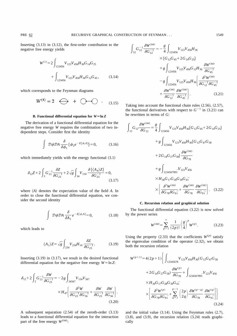
PRE 62 1549RECURSIVE GRAPHICAL CONSTRUCTION OF FEYNMAN . . .
~3.25!
which is iterated starting from ~3.15!. In analogy to ~2.64!, this recursion relation can be cast in a closed diagrammatic way byusing the alternative graphical rules ~2.63!:
~3.26!
We illustrate the procedure of solving the recursion relation ~3.25! by constructing the three-loop vacuum diagrams. Applyingone or two functional derivatives to ~3.15!, we have
~3.27!
This is inserted into ~3.25! to yield the three-loop diagramsshown in Table IV with their multiplicities. The table alsocontains the subsequent four-loop results, which we shall notderive here in detail. Observe that the multiplicity of a con-nected vacuum diagram in the f2A theory is given by aformula similar to ~2.10! in the f4 theory:
M f2AE50
5
~2p !!4p
2!S1DN. ~3.28!
Here S and D denote the number of self- and double connec-tions, and N represents again the number of vertex permuta-tions leaving the vacuum diagram unchanged.
The connected vacuum diagrams of the f2A theory inTable IV can, of course, be converted to corresponding onesof the f4 theory in Table I, by shrinking wiggly lines to apoint and dividing the resulting multiplicity by 3 in accor-dance with ~3.10!. This relation between connected vacuumdiagrams in f4 and f2A theory is emphasized by the num-bering used in Table IV. For instance, the shrinking convertsthe five diagrams 4.1–4.5 in Table IV to the diagram 4 inTable I. Taking into account the different combinatorial fac-tors in the expansion ~2.6! and ~3.23! as well as the factor 3in the shrinkage ~3.10!, the multiplicity M f4
E50 of a f4 dia-gram results from the corresponding one M f2A
E50 of the f2Apartner diagrams via the rule
M f4E50
5
1
~2p21 !!!M f2A
E50. ~3.29!
IV. COMPUTER GENERATION OF DIAGRAMS
Continuing the solution of the graphical recursion rela-tions ~2.61! and ~3.25! to higher loops becomes an arduoustask. We therefore automatize the procedure by computeralgebra. Here we restrict ourselves to the f4 theory becauseof its relevance for critical phenomena.
A. Matrix representation of diagrams
To implement the procedure on a computer we must rep-resent Feynman diagrams in the f4 theory by algebraic sym-bols. For this we use matrices as defined in Refs. @8–10#. Letp be the number of vertices of a given diagram and labelthem by indices from 1 to p. Set up an adjacency matrix Mwhose elements M i j ~0<i , j<p! specify the number of linesjoining the vertices i and j. The diagonal elements M ii (i.0) count the number of self-connections of the ith vertex.External lines of a diagram are labeled as if they were con-nected to a single additional dummy vertex with number 0.The matrix element M 00 is set to zero by convention. Theoff-diagonal elements lie in the interval 0<M i j<4, whilethe diagonal elements for i.0 are restricted by 0<M ii<2.We observe that the sum of the matrix elements M i j in eachbut the zeroth row or column equals 4, where the diagonalelements count twice,
(j50
p
M i j1M ii5(j50
p
M j i1M ii54. ~4.1!
The matrix M is symmetric and is thus specified by
1550 PRE 62KLEINERT, PELSTER, KASTENING, AND BACHMANN
(p11)(p12)/221 elements. Each matrix characterizes aunique diagram and determines its multiplicity via formula~2.28!. From the matrix M we read off directly the number ofself-, double, triple, fourfold connections S, D, T, F and thenumber of external legs E5S i51
p M 0i . It also permits us tocalculate the number N. For this we observe that the matrixM is not unique, since so far the vertex numbering is arbi-trary. In fact, N is the number of combined permutations ofvertices and external lines that leave the matrix M un-changed @compare to the statement after ~2.28!#. If nM de-notes the number of different matrices representing the samediagram, the number N is given by
N5
p!
nM)i51
p
M 0i!, ~4.2!
where the matrix elements M 0i count the number of externallegs connected to the ith vertex. One way to determine thenumber nM is to repeatedly perform the p(p21)/2 ex-changes of pairs of rows and columns except the zeroth ones,until no new matrix is generated anymore. For larger matri-ces this way of determining nM is quite tedious. Below wewill give a better approach. Inserting Eq. ~4.2! into the for-mula ~2.28!, we obtain the multiplicity of the diagram repre-sented by M. This may be used to crosscheck the multiplici-ties obtained before when solving the graphical recursionrelation ~2.61!.
So far, the vertex numbering has been arbitrary, makingthe matrix representation of a diagram nonunique. Toachieve uniqueness, we customize to our problem the proce-dure introduced in @11#. First we group the vertices in a
given diagram into different classes, which are defined bythe four tuples ~E, S, D, T! containing the number of externallegs, self-, double, and triple connections of a vertex. Theclasses are sorted by increasing numbers of E, then S, then D,then T. In general, there can still be vertices that coincide inall four numbers and whose ordering is therefore still arbi-trary. To achieve unique ordering among these vertices, weassociate with each matrix a number whose digits are com-posed of the matrix elements M i j(0< j<i<p), i.e., we formthe number with the (p11)(p12)/221 elements
M 10M 11uM 20M 21M 22uM 30M 31M 32M 33u. . .M pp . ~4.3!
To guide the eye, we have separated the digits stemmingfrom different rows by vertical lines. The smallest of thesenumbers compatible with the vertex ordering introducedabove is chosen to represent the diagram uniquely. Insteadwe could have also allowed all vertex permutations and iden-tified the number ~4.3! with a unique representation of agiven diagram. However, for most diagrams containing sev-eral vertices, this would drastically inflate the number of ad-missible matrices and therefore the effort for finding aunique representation.
Now we can also give an improved procedure for findingnM . Let nM8 be the number of different matrices compatiblewith the vertex ordering by the four tuples introduced above.Let there be c classes of vertices and k1 , . . . ,kc vertices be-longing to each class. Then we have
nM5
p!
) j51c k j!
nM8 ~4.4!
TABLE IV. Connected vacuum diagrams and their multiplicities of the f2A theory up to four loops. Each diagram is characterized bythe vector ~S, D; N! whose components specify the number of self- and double connections as well as the vertex permutations leaving thevacuum diagram unchanged, respectively.
PRE 62 1551RECURSIVE GRAPHICAL CONSTRUCTION OF FEYNMAN . . .
or, together with ~4.2!,
N5
1
nM8S )
j51
c
k j! D S )i51
p
M 0i! D . ~4.5!
As an example, consider the following diagram of thefour-point function with p53 vertices:
~4.6!
Its vertices are grouped into c52 classes with k152 verticesbelonging to the first class characterized by the four tuple(E ,S ,D ,T)5(1,0,1,0) and k251 vertex belonging to thesecond class (E ,S ,D ,T)5(2,0,0,0). When labeling the ver-tices in view of the unique matrix representation, the vertexin the second class comes last because of the higher numberof external legs. Exchanging the other two vertices in thefirst class does not change the adjacency matrix anymore dueto the reflection symmetry of the diagram ~4.6!. Thus itsunique matrix representation reads
S 0 1 1 2
1 0 2 1
1 2 0 1
2 1 1 0
D , ~4.7!
with rows and columns indexed from 0 to 3. According toEq. ~4.3!, the matrix ~4.7! yields the number
10u120u2110. ~4.8!
As there is nm8 51 matrix compatible with the vertex orderingby the four tuples, the number N of vertex permutations ofthe diagram ~4.6! is determined from ~4.5! as 4 ~compare thecorresponding entry in Table III!.
A more complicated example is provided by the followingdiagram of the two-point function with p54 vertices:
~4.9!
Here we have again c52 classes, the first one is(E ,S ,D ,T)5(0,0,2,0) with k152 vertices and the secondone (E ,S ,D ,T)5(1,0,1,0) with k252 vertices. Exchangingboth vertices in each class leads now to nM8 52 differentmatrices
S 0 0 0 1 1
0 0 2 2 0
0 2 0 0 2
1 2 0 0 1
1 0 2 1 0
D , S 0 0 0 1 1
0 0 2 0 2
0 2 0 2 0
1 0 2 0 1
1 2 0 1 0
D .
~4.10!
For the unique matrix representation we have to choose thelast matrix as it leads to the smaller number
00u020u1020u12010. ~4.11!
From Eq. ~4.5! we read off that the number N of vertexpermutations of the diagram ~4.9! is 2 ~compare the corre-sponding entry in Table II!.
The matrix M contains, of course, all information on thetopological properties of a diagram @9,10#. For this we definethe submatrix M by removing the zeroth row and columnfrom M. This allows us to recognize the connectedness of adiagram: A diagram is disconnected if there is a vertex num-bering for which M is a block matrix. Furthermore a vertexis a cut vertex, i.e., a vertex which links two otherwise dis-connected parts of a diagram, if the matrix M has an almostblock form for an appropriate numbering of vertices in whichthe blocks overlap only on some diagonal element M ii , i.e.,the matrix M takes block form if the ith row and column areremoved. Similarly, the matrix M allows us to recognize aone-particle-reducible diagram, which falls into two piecesby cutting a certain line. Removing a line amounts to reduc-ing the associated matrix elements in the submatrix M byone. If the resulting matrix M has block form for a certainvertex ordering, the diagram is one-particle reducible.
B. Practical generation
We are now prepared for the computer generation ofFeynman diagrams. First the vacuum diagrams are generatedfrom the recursion relation ~2.61!. From these the diagramsof the connected two- and four-point functions are obtainedby cutting or removing lines. We used a MATHEMATICA pro-gram to perform this task. The resulting unique matrix rep-resentations of the diagrams up to the order p54 are listedin Tables V–VII. They are the same as those derived beforeby hand in Tables I–III. Higher-order results up to p56,containing all diagrams that are relevant for the five-looprenormalization of f4 theory in d542e dimensions@10,20#, are made available on the internet @19#, where alsothe program can be found.
1. Connected vacuum diagrams
The computer solution of the recursion relation ~2.61! ne-cessitates to keep an exact record of the labeling of externallegs of intermediate diagrams which arise from differentiat-ing a vacuum diagram with respect to a line once or twice.To this end we have to extend our previous matrix represen-tation of diagrams where the external legs are labeled as ifthey were connected to a simple additional vertex with num-ber 0. For each matrix representing a diagram we define anassociated vector that contains the labels of the external legsconnected to each vertex. This vector has the length of thedimension of the matrix and will be added to the matrix as anextra left column, separated by a vertical line. Consider, asan example, the diagram ~4.6! of the four-point function withp53 vertices, where the spatial indices 1, 2, 3, 4 are as-signed in a particular order:
~4.12!
In our extended matrix notation, such a diagram can be rep-resented in total by six matrices:
1552 PRE 62KLEINERT, PELSTER, KASTENING, AND BACHMANN
S $ % 0 2 1 1
$1,2% 2 0 1 1
$3% 1 1 0 2
$1% 1 1 2 0
D , S $ % 0 1 2 1
$3% 1 0 1 2
$1,2% 2 1 0 1
$4% 1 2 1 0
D , S $ % 0 1 1 2
$3% 1 0 2 1
$4% 1 2 0 1
$1,2% 2 1 1 0
D ,
S $ % 0 2 1 1
$1,2% 2 0 1 1
$4% 1 1 0 2
$3% 1 1 2 0
D , S $ % 0 1 2 1
$4% 1 0 1 2
$1,2% 2 1 0 1
$3% 1 2 1 0
D , S $ % 0 1 1 2
$4% 1 0 2 1
$3% 1 2 0 1
$1,2% 2 1 1 0
D . ~4.13!
When constructing of the vacuum diagrams from the recursion relation ~2.61!, starting from the two-loop diagram ~2.62!, wehave to represent three different elementary operations in our extended matrix notation:
~i! Taking one or two derivatives of a vacuum diagram with respect to a line. For example, we apply this operation to thevacuum diagram 2 in Table I
TABLE V. Unique matrix representation of all connected vacuum diagrams of f4 theory up to the orderp54. The number in the first column corresponds to their graphical representation in Table I. The matrixelements M i j represent the numbers of lines connecting two vertices i and j, omitting M i050 for simplicity.The running numbers of the vertices are listed on top of each column in the first two rows. The furthercolumns contain the vector ~S, D, T, F; N! characterizing the topology of the diagram, the multiplicity M, andthe weight W5M /@(4!)pp!# . The graphs are ordered according to their number of self-connections, thendouble connections, then triple connections, then fourfold connections, then the number ~4.3!.
PRE 62 1553RECURSIVE GRAPHICAL CONSTRUCTION OF FEYNMAN . . .
~4.14!
This has the matrix representation
d2
dG12dG34S $% 0 0 0
$% 0 0 4
$% 0 4 0D 52
d
dG12F S $% 0 1 1
$3% 1 0 3
$4% 1 3 0D 1S $% 0 1 1
$4% 1 0 3
$3% 1 3 0D G
53F S $% 0 2 2
$1,3% 2 0 2
$2,4% 2 2 0D 1S $% 0 2 2
$2,3% 2 0 2
$1,4% 2 2 0D 1S $% 0 2 2
$1,4% 2 0 2
$2,3% 2 2 0D
1S $% 0 2 2
$2,4% 2 0 2
$1,3% 2 2 0D G . ~4.15!
TABLE VI. Unique matrix representation of all diagrams of the connected two-point function of f4 theory up to the order p54. Thenumbers in the first column correspond to their graphical representation in Table II. The matrix elements M i j represent the numbers of linesconnecting two vertices i and j. The running numbers of the vertices are listed on top of each column in the first two rows. The furthercolumns contain the vector ~S, D, T; N! characterizing the topology of the diagram, the multiplicity M, and the weight W5M /@(4!)pp!# . Thegraphs are ordered according to their number of self-connections, then double connections, then triple connections, then the number ~4.3!.
1554 PRE 62KLEINERT, PELSTER, KASTENING, AND BACHMANN
The first and fourth matrix as well as the second and third matrix represent the same diagram in ~4.14!, as can be seen bypermuting rows and columns of either matrix.
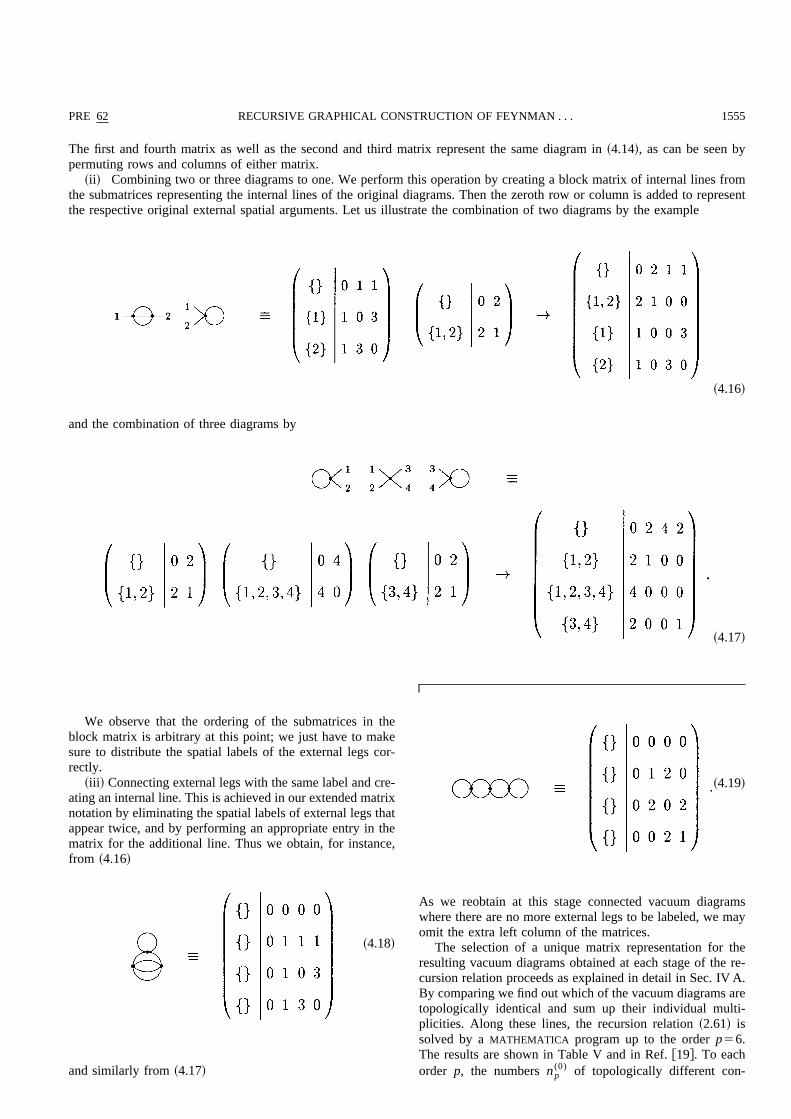
~ii! Combining two or three diagrams to one. We perform this operation by creating a block matrix of internal lines fromthe submatrices representing the internal lines of the original diagrams. Then the zeroth row or column is added to representthe respective original external spatial arguments. Let us illustrate the combination of two diagrams by the example
~4.16!
and the combination of three diagrams by
~4.17!
We observe that the ordering of the submatrices in theblock matrix is arbitrary at this point; we just have to makesure to distribute the spatial labels of the external legs cor-rectly.
~iii! Connecting external legs with the same label and cre-ating an internal line. This is achieved in our extended matrixnotation by eliminating the spatial labels of external legs thatappear twice, and by performing an appropriate entry in thematrix for the additional line. Thus we obtain, for instance,from ~4.16!
~4.18!
and similarly from ~4.17!
~4.19!
As we reobtain at this stage connected vacuum diagramswhere there are no more external legs to be labeled, we mayomit the extra left column of the matrices.
The selection of a unique matrix representation for theresulting vacuum diagrams obtained at each stage of the re-cursion relation proceeds as explained in detail in Sec. IV A.By comparing we find out which of the vacuum diagrams aretopologically identical and sum up their individual multi-plicities. Along these lines, the recursion relation ~2.61! issolved by a MATHEMATICA program up to the order p56.The results are shown in Table V and in Ref. @19#. To eachorder p, the numbers np
(0) of topologically different con-
PRE 62 1555RECURSIVE GRAPHICAL CONSTRUCTION OF FEYNMAN . . .

nected vacuum diagrams are
~4.20!
A direct comparison with other, already established com-puter programs like FEYNARTS @1–3# or QGRAF @4,5# showsthat the automatization of the graphical recursion relation~2.61! in terms of our MATHEMATICA code is inefficient. Ac-cording to our experience, the major part of the CPU timeneeded for the generation of high-loop order diagrams is de-voted to the reordering of vertices to obtain the unique ma-trix representation of a diagram—a problem faced also byother graph-generating methods. After implementation of adedicated algorithm for the vertex ordering written for in-stance in Fortran or C, we would therefore expect CPU times
for the time-consuming high-loop diagrams which are com-parable to those of other programs.
2. Two- and four-point functions G12 and G1234c
from cutting lines
Having found all connected vacuum diagrams, we derivefrom these the diagrams of the connected two- and four-pointfunctions by using the relations ~2.18! and ~2.25!. In thematrix representation, cutting a line is essentially identical toremoving a line as explained above, except that we nowinterpret the labels that represent the external spatial labels assitting on the end of lines. Since we are not going to distin-guish between trivially ‘‘crossed’’ diagrams that are relatedby exchanging external labels in our computer implementa-tion, we need no longer carry around external spatial labels.Thus we omit the extra left column of the matrix represent-ing a diagram when generating vacuum diagrams. As an ex-ample, consider cutting a line in diagram 3 inTable I
~4.21!
which has the matrix representation
2
d
dG21 S 0 0 0
0 1 2
0 2 1D 52S 0 1 1
1 1 1
1 1 1D 1S 0 2 0
2 0 2
0 2 1D 1S 0 0 2
0 1 2
2 2 0D . ~4.22!
Here the plus signs and multiplication by 2 have a set theoretical meaning and are not to be understood as matrix algebraoperations. The last two matrices represent, incidentally, the same diagram in ~4.21! as can be seen by exchanging the last tworows and columns of either matrix.
To create the connected four-point function, we also have to consider second derivatives of vacuum diagrams with respectto G21. If an external line is cut, an additional external line will be created, which is not connected to any vertex. It can beinterpreted as a self-connection of the zeroth vertex, which collects the external lines. This may be accommodated in thematrix notation by letting the matrix element M 00 count the number of lines not connected to any vertex. For example, takingthe derivative of the first diagram in Eq. ~4.21! gives
~4.23!
with the matrix notation
2
d
dG21 S 0 1 1
1 1 1
1 1 1D 5S 0 3 1
3 0 1
1 1 1D 1S 0 1 3
1 1 1
3 1 0D
1S 0 2 2
2 1 0
2 0 1D 12S 1 1 1
1 1 1
1 1 1D .
~4.24!
The first two matrices represent the same diagram as can beseen from Eq. ~4.23!. The last two matrices in Eq. ~4.24!correspond to disconnected diagrams: the first one becauseof the absence of a connection between the two vertices, thesecond one because of the disconnected line represented bythe entry M 0051. In the full expression for the two-loopcontribution G1234
c ,(2) to the four-point function in Eq. ~2.25! alldisconnected diagrams arising from cutting a line in G12
(2) arecanceled by diagrams resulting from the sum. Therefore wemay omit the sum, take only the first term and discard alldisconnected diagrams it creates. This is particularly usefulfor treating low orders by hand. If we include the sum, weuse the prescription of combining diagrams into one as de-
1556 PRE 62KLEINERT, PELSTER, KASTENING, AND BACHMANN
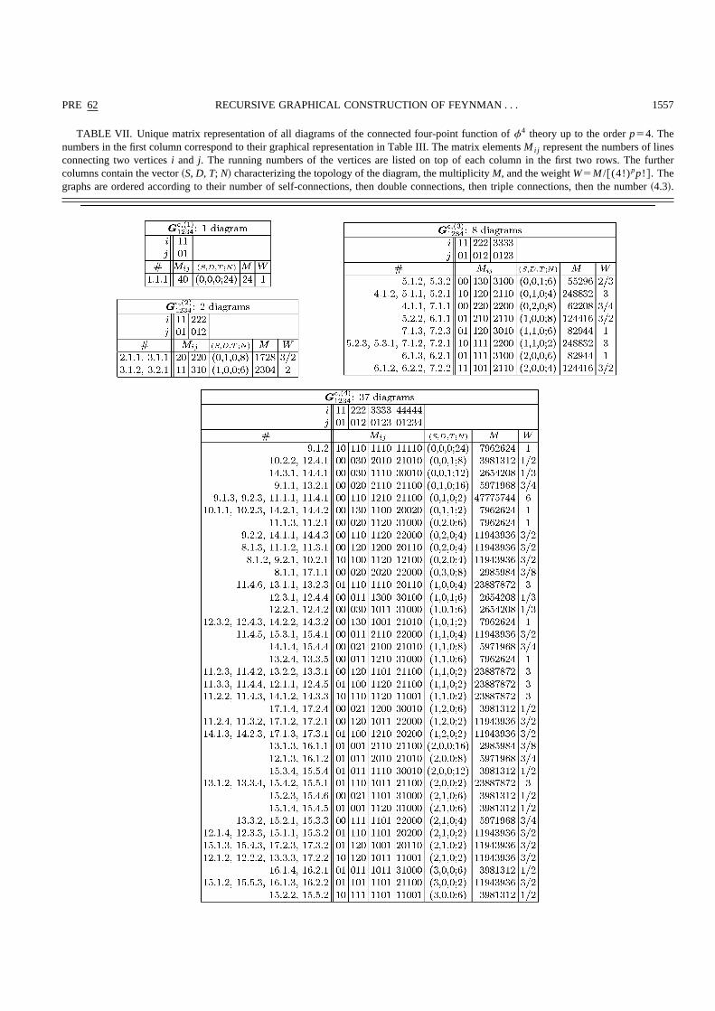
TABLE VII. Unique matrix representation of all diagrams of the connected four-point function of f4 theory up to the order p54. Thenumbers in the first column correspond to their graphical representation in Table III. The matrix elements M i j represent the numbers of linesconnecting two vertices i and j. The running numbers of the vertices are listed on top of each column in the first two rows. The furthercolumns contain the vector ~S, D, T; N! characterizing the topology of the diagram, the multiplicity M, and the weight W5M /@(4!)pp!# . Thegraphs are ordered according to their number of self-connections, then double connections, then triple connections, then the number ~4.3!.
PRE 62 1557RECURSIVE GRAPHICAL CONSTRUCTION OF FEYNMAN . . .
scribed above in Sec. IV B, except that we now omit theextra vector with the labels of spatial arguments.
3. Two- and four-point functions G12 and G1234c
from removing lines
Instead of cutting lines of connected vacuum diagramsonce or twice, the perturbative coefficients of G12 and G1234
c
can also be obtained graphically by removing lines. Indeed,from ~2.16!, ~2.44!, ~2.54!, and ~2.56! we get for the two-point function
G125G1212E34
G13G24
dW ~ int!
dG34, ~4.25!
so that we have for p.0
G12~p !
52E34
G13G24
dW ~p !
dG34~4.26!
at our disposal to compute the coefficients G12(p) from remov-
ing one line in the connected vacuum diagrams W (p) in allpossible ways. The corresponding matrix operations areidentical to the ones for cutting a line so that in this respectthere is no difference between both procedures to obtainG12 .
Combining ~4.25! with ~2.12!, ~2.23!, and ~2.56!, we getfor the connected four-point function
G1234c
54E5678
G15G26G37G48
d2W ~ int!
dG56dG78
24E5678
G15G27~G36G481G46G38!dW ~ int!
dG56
dW ~ int!
dG78,
~4.27!
which is equivalent to
G1234c ,~p !
54E5678
G15G26G37G48
d2W ~p !
dG56dG78
24 (q51
p21 S pq D E
5678G15G27~G36G481G46G38!
3
dW ~q !
dG56
dW ~p2q !
dG78. ~4.28!
Again, the sum serves only to subtract disconnected dia-grams that are created by the first term, so we may choose toomit the second term and to discard the disconnected dia-grams in the first term.
Now the problem of generating diagrams is reduced to thegeneration of vacuum diagrams and subsequently takingfunctional derivatives with respect to G12 . An advantage ofthis approach is that external lines do not appear at interme-diate steps. So when one uses the cancellation of discon-nected terms as a cross check, there are less operations to beperformed than with cutting. At the end one just interpretsexternal labels as sitting on external lines. Since all necessaryoperations on matrices have already been introduced, we
omit examples here and just note that we can again omitexternal labels if we are not distinguishing between trivially‘‘crossed’’ diagrams.
The generation of diagrams of the connected two- andfour-point functions has been implemented in both possibleways. Cutting or removing one or two lines in the connectedvacuum diagrams up to the order p56 leads to the followingnumbers np
(2) and np(4) of topologically different diagrams of
G12(p) and G1234
c ,(p) :
~4.29!
V. OUTLOOK
Using the example of f4 and f2A theory, we have devel-oped in this work a new method to generate all topologicallydifferent Feynman diagrams together with their proper mul-tiplicities without any combinatorial considerations. Solvinga graphical recursion relation leads to the connected vacuumdiagrams and a subsequent cutting of their lines results in theconnected diagrams. Although our automatization in termsof a MATHEMATICA code @19# turned out to be inefficient incomparison with other, already established programs likeFEYNARTS @1–3# or QGRAF @4,5#, the construction method assuch is conceptually attractive as it immediately followsfrom the functional integral approach to field theory. As de-tailed in Sec. IV B, we expect that a sophisticated implemen-tation of our program will be as efficient as existing codes.
In separate publications our method is applied to generatethe Feynman diagrams of quantum electrodynamics @21# andone-particle irreducible diagrams in the ordered phase of f4
theory, where the energy functional contains a mixture ofcubic and quartic interactions @22,23#. The work @22# alsosuggests the capability of our new method beyond a meregeneration of graphs. For example, a formal proof of the factthat W generates connected graphs and that the effective en-ergy G generates one-particle irreducible graphs could be es-tablished. Also, a simple all-orders resummation of perturba-tion theory is presented there. We believe that our methodhas great potential in formalizing physically interesting re-summations without concern over combinatorics of graphsexplicitly, a frequent source of errors in the history of resum-mations.
It is hoped that our method will eventually be combinedwith efficient numerical algorithms for actually evaluatingFeynman diagrams, e.g., for a more accurate determinationof universal quantities in critical phenomena.
ACKNOWLEDGEMENTS
We are grateful to Dr. Bruno van den Bossche and FlorianJasch for contributing various useful comments. M.B. andB.K. acknowledge support by the Studienstiftung des deut-schen Volkes and the Deutsche Forschungsgemeinschaft~DFG!, respectively.
1558 PRE 62KLEINERT, PELSTER, KASTENING, AND BACHMANN
@1# J. Kulbeck, M. Bohm, and A. Denner, Comput. Phys. Com-mun. 60, 165 ~1991!.
@2# T. Hahn, e-print hep-ph/9905354.@3# http://www-itp.physik.uni-karlsruhe.de/feynarts@4# P. Nogueira, J. Comput. Phys. 105, 279 ~1993!.@5# ftp://gtae2.ist.utl.pt/pub/qgraf@6# H. Kleinert, Fortschr. Phys. 30, 187 ~1982!.@7# H. Kleinert, Fortschr. Phys. 30, 351 ~1982!.@8# B. R. Heap, J. Math. Phys. 7, 1582 ~1966!.@9# J. Neu, M.S. thesis ~in German!, Freie Universitat Berlin,
1990.@10# H. Kleinert and V. Schulte-Frohlinde, Critical Properties of f4
Theories ~World Scientific, Singapore, 2000!.@11# J. F. Nagle, J. Math. Phys. 7, 1588 ~1966!.@12# B. Kastening, Phys. Rev. D 54, 3965 ~1996!.@13# B. Kastening, Phys. Rev. D 57, 3567 ~1998!.@14# S. A. Larin, M. Monnigmann, M. Strosser, and V. Dohm,
Phys. Rev. B 58, 3394 ~1998!.@15# D. J. Amit, Field Theory, the Renormalization Group and
Critical Phenomena ~McGraw-Hill, New York, 1978!.@16# C. Itzykson and J.-B. Zuber, Quantum Field Theory ~McGraw-
Hill, New York, 1985!.@17# J. Zinn-Justin, Quantum Field Theory and Critical Phenom-
ena, 3rd ed. ~Oxford University, New York, 1996!.@18# H. Kleinert, Gauge Fields in Condensed Matter, Vol. I, Super-
flow and Vortex Lines ~World Scientific, Singapore, 1989!.@19# http://www.physik.fu-berlin.de/~kleinert/294/programs.@20# H. Kleinert, J. Neu, V. Schulte-Frohlinde, K. G. Chetyrkin,
and S. A. Larin, Phys. Lett. B 272, 39 ~1991!; 319, 545~E!
~1993!.@21# M. Bachmann, H. Kleinert, and A. Pelster, Phys. Rev. D 61,
085017 ~2000!.@22# B. Kastening, Phys. Rev. E 61, 3501 ~2000!.@23# A. Pelster and H. Kleinert, e-print hep-th/0006153.
PRE 62 1559RECURSIVE GRAPHICAL CONSTRUCTION OF FEYNMAN . . .