Rectangular Layouts and Contact Graphsadambuchsbaum.com/papers/rectlay.pdf · Rectangular Layouts and Contact Graphs ... architectural design, ... Previous works considered concepts

Rectangular Layouts and Contact Graphs

ADAM L. BUCHSBAUM and EMDEN R. GANSNER and CECILIA M. PROCOPIUC

AT&T Labs

and

SURESH VENKATASUBRAMANIAN

University of Utah

Contact graphs of isothetic rectangles unify many concepts from applications including VLSI andarchitectural design, computational geometry, and GIS. Minimizing the area of their correspondingrectangular layouts is a key problem. We study the area-optimization problem and show that itis NP-hard to find a minimum-area rectangular layout of a given contact graph. We presentO(n)-time algorithms that construct O(n2)-area rectangular layouts for general contact graphsand O(n log n)-area rectangular layouts for trees. (For trees, this is an O(log n)-approximationalgorithm.) We also present an infinite family of graphs (rsp., trees) that require Ω(n2) (rsp.,Ω(n log n)) area.

We derive these results by presenting a new characterization of graphs that admit rectangularlayouts using the related concept of rectangular duals. A corollary to our results relates the classof graphs that admit rectangular layouts to rectangle of influence drawings.

Categories and Subject Descriptors: F.2.2 [Nonnumerical Algorithms and Problems]: Com-putations on discrete structures; G.2.2 [Graph Theory]: Graph algorithms

General Terms: Algorithms, Theory

Additional Key Words and Phrases: contact graphs, rectangular duals, rectangular layouts

1. INTRODUCTION

Given a set of objects in some space, the associated contact graph contains a vertexfor each object and an edge implied by each pair of objects that touch in someprescribed fashion. While contact graphs have been extensively studied for objectssuch as curves, line segments, and even strings (surveyed by Hlineny [1998] andHlineny and Kratochvıl [2001]), as has the more general class of intersection graphs(surveyed by Brandstadt et al. [1999] and McKee and McMorris [1999]), the litera-ture on closed shapes is relatively sparse. Koebe’s Theorem [1936] states that anyplanar graph (and only a planar graph) can be expressed as the contact graph ofdisks in the plane. (This result was lost and recently rediscovered independently by

Authors’ addresses: Adam L. Buchsbaum, Emden R. Gansner, and Ceclia M. Pro-copiuc, AT&T Labs, Shannon Laboratory, 180 Park Ave., Florham Park, NJ 07932, USA;alb,erg,[email protected]. Suresh Venkatasubramanian, School of Computing, 50 S. Cen-tral Campus Drive, Salt Lake City, UT 84112, USA; [email protected] work of the fourth author was completed while he was a member of AT&T Labs.Permission to make digital/hard copy of all or part of this material without fee for personalor classroom use provided that the copies are not made or distributed for profit or commercialadvantage, the ACM copyright/server notice, the title of the publication, and its date appear, andnotice is given that copying is by permission of the ACM, Inc. To copy otherwise, to republish,to post on servers, or to redistribute to lists requires prior specific permission and/or a fee.c© 2007 ACM 0000-0000/2007/0000-0001 $5.00

ACM Journal Name, Vol. V, No. N, October 2007, Pages 1–29.

2 · Adam L. Buchsbaum et al.

Andreev and Thurston; Sachs [1994] provides a history.) More recently, de Fraysseixet al. [1994] show that any planar graph can be represented as a triangle contactgraph but not vice-versa. In this paper, we consider contact graphs of isotheticrectangles.

Contact graphs of rectangles find critical applications in areas including VLSIdesign [Lai and Leinwand 1988; Sur-Kolay and Bhattacharya 1988; 1991; Taniet al. 1991; Yeap and Sarrafzadeh 1995], architectural design [Steadman 1976],and, in other formulations, computational geometry [de Berg et al. 1992; Overmarsand Wood 1988] and geographic information systems [Gabriel and Sokal 1969].Previous works considered concepts similar to contact graphs but used a varietyof notions like rectangular duality [He 1993; Kozminski and Kinnen 1985; 1988;Lai and Leinwand 1990] and concepts from graph drawing such as orthogonal,rectilinear, visibility, and proximity layouts [Di Battista et al. 1994; Di Battistaet al. 1999; Rosenstiehl and Tarjan 1986] as well as rectangular drawings [He 2001;Rahman et al. 1998; 2000; Rahman et al. 2004] to achieve their results. Our workis the first to deal directly with contact graphs of rectangles, yielding a simplerfoundation for study.

We call a collection of rectangles that realizes a given contact graph G a rectangu-lar layout: a set of disjoint, isothetic rectangles corresponding to the vertices of G,such that two rectangles are adjacent if and only if the implied edge exists in G. Theassociated optimization problem is to find a rectangular layout minimizing somecriterion such as area, width, or height. This problem is inherently intriguing, withmany enticing subproblems and variations. It arises in practice in the design of aninterface to a relational database system used in AT&T to allow customers to modeland administer the equipment and accounts in their telecommunications networks.This system allows users to specify their own schemas using entity-relationshipmodels [Ramakrishnan and Gehrke 2000]. The system then presents the databaseentities as rectangular buttons. Clicking on a button provides information relatedto the corresponding entity type: e.g., detailed descriptions of the entity attributesor information about specific records. Experience indicates the benefit of juxtapos-ing buttons that correspond to related entities. Viewing the database schema asthe obvious graph, with entities as vertices and relations as edges, leads to rect-angular layouts. Solving the related optimization problems would automate thispart of tailoring the interface to the schema, of significant benefit as otherwise eachcustomer’s interface must be built manually.

We solve several important problems concerning rectangular layouts. We give anew characterization of planar graphs that admit rectangular layouts in terms ofthose that can be embedded without filled triangles. En route, we unify a numberof different lines of research in this field. We show a suite of results concerningthe hardness of finding optimal layouts; design algorithms to construct layouts ongraphs, and, with better area bounds, trees; and present some worst-case area lowerbounds. We detail these results at the end of this section.

1.1 Relationship to Prior Work

Rectangular layouts are dual concepts to rectangle drawings of planar graphs, whichare straight-line, isothetic embeddings with only rectangular faces. Recent work onrectangular drawings [Rahman et al. 1998; Rahman et al. 2004] and the relatedACM Journal Name, Vol. V, No. N, October 2007.

Rectangular Layouts and Contact Graphs · 3

box-rectangular drawings [He 2001; Rahman et al. 2000] culminates with Rah-man, Nishizeki, and Ghosh’s [2004] linear-time algorithm for finding a rectangulardrawing of any planar graph if one exists. In a rectangular layout, the rectan-gles themselves correspond to vertices. While the two concepts are more or lessdual to each other, moving between them can be highly technical. In particular,the machinery to find rectangular drawings of graphs that are not three-connectedis complex. Our contribution gives a direct method for constructing rectangularlayouts, and we handle cases of low connectivity easily.

Rectangular layouts are closely related to rectangular duals, which are like lay-outs except that a rectangular dual must form a dissection of its enclosing rectangle;i.e., it allows no gaps between rectangles. Rectangular duals have a rich history,including much work on characterizing graphs that admit rectangular duals [He1993; Kozminski and Kinnen 1985; 1988; Lai and Leinwand 1990], transformingthose that do not by adding new vertices [Accornero et al. 2000; Lai and Leinwand1988], and constructing rectangular duals in linear time [Bhasker and Sahni 1988;He 1993; Kant and He 1997]. The proscription of gaps, however, severely limitsthe class of graphs that admit rectangular duals; for example, paths are the onlytrees that have such duals. In general, any (necessarily planar) graph admittinga rectangular dual must be internally triangulated, but no such restriction appliesto layouts. This simple distinction yields many advantages to layouts over duals.The cleaner, less specified definition of layouts characterizes a class of graphs thatis both more general (including all trees, for example) and also much simpler toformalize. When we discuss area, we will also show that while different variationsof rectangular layouts have different degrees of area monotonicity under graph aug-mentation, rectangular duals do not enjoy any such monotonicity: a small graphmight require a significantly larger dual than a larger graph. Additionally, thereare graphs that admit asymptotically smaller rectangular layouts than duals.

Another closely related area concerns VLSI floorplanning, in which an initial con-figuration of rectangles (usually a dissection) is given, and the goal is to rearrangeand resize the rectangles to minimize the area while preserving some properties ofthe original layout. While there is an extensive literature on floorplanning, there ismuch divergence within it as to what criteria must be preserved during minimiza-tion. These typically include minimum size constraints on the rectangles plus oneof various notions of adjacency equivalence. Stockmeyer [1983] presents one of thecleanest definitions of equivalence, preserving the notion of relative placement ofrectangles (whether one appears left of, right of, above, or below another); othercriteria include the preservation of relative area and aspect ratios [Wimer et al.1988] and that of relative lengths of abutment [Tani et al. 1991]. These worksare further classified by sliceability: a floorplan is sliceable if it can be recursivelydeconstructed by vertical and horizontal lines extending fully across the boundingbox. Minimizing the area of non-sliceable floorplans has been shown to be NP-hard under various constraints [LaPaugh 1980; Pan et al. 1996; Stockmeyer 1983],whereas area minimization of sliceable floorplans is tractable [Shi 1996; Stockmeyer1983; Yeap and Sarrafzadeh 1993]. Not all floorplans can be realized by sliceableequivalents [Sur-Kolay and Bhattacharya 1988; 1991], so work exists on isolatingand generating sliceable floorplans where possible [Yeap and Sarrafzadeh 1995] as

ACM Journal Name, Vol. V, No. N, October 2007.


well as minimizing the area of non-sliceable floorplans by various heuristics [Panet al. 1996; Tani et al. 1991; Wimer et al. 1988].

Two major facets distinguish floorplanning from area-minimization of rectangu-lar layouts. First, floorplanning seeks to minimize the area of an arrangement ofrectangles given a priori by some external process (possibly human design); rectan-gular layouts themselves are determined by corresponding contact graphs. Second,the notion of equivalence among floorplans differs from context to context, whereascontact graph adjacencies strictly identify the equivalence of rectangular layouts.Thus, there can exist different rectangular layouts of the same graph that do notrepresent equivalent floorplans, even by Stockmeyer’s definition; and converselythere can exist equivalent floorplans that are layouts for non-isomorphic graphs.Still, much work in floorplanning uses concepts from rectangular duals, so work onrectangular layouts can also contribute to this area.

Finally, also related is the idea of proximity drawings [Di Battista et al. 1994;Jaromczyk and Toussaint 1992], in which a set of objects corresponds to the verticesof a graph, with edges connecting vertices of correspondingly close objects for somedefinition of proximity. A particularly relevant special case is that of rectangle ofinfluence drawings [Liotta et al. 1998], which are (not necessarily planar) straight-line embeddings of graphs such that the isothetic rectangles induced by pairs ofvertices contain no other vertices if and only if the corresponding edges exist. Usingresults of Biedl et al. [1999], we show that graphs that admit rectangular layoutsare precisely those that admit a weaker variation of planar rectangle of influencedrawings, in which induced rectangles may be empty even if the corresponding edgesare missing from the graph; i.e., that contact graphs of rectangles also express thisvariation of rectangle of influence drawings.

1.2 Our Results

The many parallel lines of research (in different communities) in the general area ofcontact graphs of rectangles have led to overlapping (and in some cases equivalent)definitions and results. Our contributions in this paper are two-fold: we presentalgorithms for optimizing rectangular layouts and prove various hardness results,and we also prove various structural results that tie existing work together in acoherent way that produces efficient algorithms.

— We provide a new characterization of the class of graphs that admit rectan-gular layouts. This characterization is equivalent to an earlier result by Thomassen[1986] and has the added advantage of yielding an O(n)-time algorithm for checkingif a given n-vertex planar graph admits such a layout. Moreover, we can constructa layout for the input graph in O(n) time. We also prove an upper bound of O(n2)on the area of the layout, and we give a matching worst-case lower bound.

— We give an O(n)-time algorithm that constructs an O(n log n)-area layoutfor any tree. We also demonstrate a general class of trees that are flexible: i.e.,they can be laid out in linear area with any aspect ratio. Finally we show thatin general trees cannot have arbitrarily thin layouts: there exists a class of treessuch that the minimum dimension must have size Ω(log n). This bound uses solelytopological arguments and may be of independent interest. In particular, it leadsto an Ω(n log n) worst-case area lower bound, matching the upper bound of ourACM Journal Name, Vol. V, No. N, October 2007.


algorithm.— We prove that the problem of optimizing the area of a rectangular layout is

NP-hard. The proof also shows that optimizing the width given a fixed height, orvice-versa, is NP-hard.

— We show that rectangular duals can be much larger than layouts; there existsa class of graphs having O(n)-area layouts but Ω(n2)-area duals.

— Our characterization of contact graphs of rectangles in terms of filled trianglesestablishes a connection between rectangular layouts and rectangle of influencedrawings. Specifically, a corollary of our characterization is that the class of graphshaving rectangular layouts is identical to the class of graphs having planar, weak,closed rectangle of influence drawings [Biedl et al. 1999].

1.3 Paper Outline

We continue in Section 2 by introducing necessary definitions, including those forrectangular layouts themselves, and we also state some useful lemmas. In Section 3we present our new characterization of graphs that admit rectangular layouts. Weuse this characterization in Section 4 to design our linear-time algorithm for con-structing O(n2)-area rectangular layouts, and we show matching worst-case lowerbounds. In Section 5 we present improved results for trees. We present hardnessresults in Section 6, and we conclude in Section 7.

2. DEFINITIONS

Throughout, we assume without loss of generality that all graphs are connectedand have at least 4 vertices. For a given graph G = (V,E), define n = |V | andm = |E|. We say G′ = (V ′, E′) is a subgraph of G if V ′ ⊆ V and E′ ⊆ E; G′ is aproper subgraph of G if G′ is a subgraph of G and G′ 6= G.

A graph G is k-connected if the removal of any set of k − 1 vertices leaves theremainder of G connected. A separating triangle of G is a 3-vertex cycle whoseremoval disconnects the remainder of G. For an arbitrary but fixed embeddingof a planar graph, a filled triangle is defined to be a length-3 cycle with at leastone vertex inside the induced region. Note that an embedding of a graph mighthave a filled triangle but no separating triangle (e.g., any embedding of K4) andvice-versa. A cubic graph is a regular degree-3 graph. A planar triangulation is aplanar graph in which all faces are bounded by 3-vertex cycles. Whitney’s [1933] 2-Isomorphism Theorem implies that a planar triangulation has a unique embeddingup to stereographic projection, which preserves the facial structure, so it is well-defined to talk about a planar graph G itself being a triangulation (or triangulated)as opposed to some specific embedding of G being triangulated. Note also thata planar triangulation G has a planar dual, denoted G∗, which is unique up toisomorphism. Clearly, any 4-connected graph has no separating triangle; for planartriangulations, the converse holds as well.

Lemma 2.1. A planar triangulation G is 4-connected if and only if G has noseparating triangles.

Kozminski and Kinnen [1985, Lem. 1] state Lemma 2.1 in terms of a fixed em-bedding, but the above remarks obviate the issue of fixed embeddings for planar



b

cd

ab

cd

b

cd

ab

cd

a

(a)

a

(b)

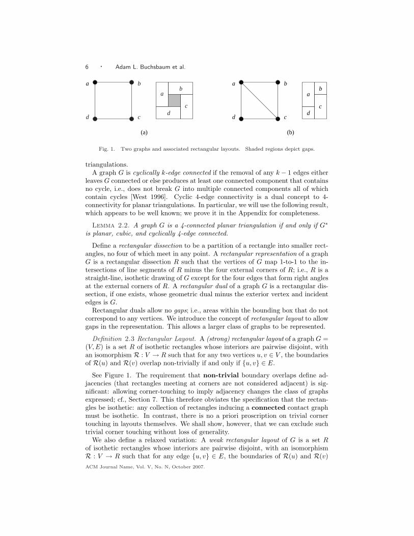
Fig. 1. Two graphs and associated rectangular layouts. Shaded regions depict gaps.

triangulations.A graph G is cyclically k-edge connected if the removal of any k − 1 edges either

leaves G connected or else produces at least one connected component that containsno cycle, i.e., does not break G into multiple connected components all of whichcontain cycles [West 1996]. Cyclic 4-edge connectivity is a dual concept to 4-connectivity for planar triangulations. In particular, we will use the following result,which appears to be well known; we prove it in the Appendix for completeness.

Lemma 2.2. A graph G is a 4-connected planar triangulation if and only if G∗

is planar, cubic, and cyclically 4-edge connected.

Define a rectangular dissection to be a partition of a rectangle into smaller rect-angles, no four of which meet in any point. A rectangular representation of a graphG is a rectangular dissection R such that the vertices of G map 1-to-1 to the in-tersections of line segments of R minus the four external corners of R; i.e., R is astraight-line, isothetic drawing of G except for the four edges that form right anglesat the external corners of R. A rectangular dual of a graph G is a rectangular dis-section, if one exists, whose geometric dual minus the exterior vertex and incidentedges is G.

Rectangular duals allow no gaps; i.e., areas within the bounding box that do notcorrespond to any vertices. We introduce the concept of rectangular layout to allowgaps in the representation. This allows a larger class of graphs to be represented.

Definition 2.3 Rectangular Layout. A (strong) rectangular layout of a graph G =(V, E) is a set R of isothetic rectangles whose interiors are pairwise disjoint, withan isomorphism R : V → R such that for any two vertices u, v ∈ V , the boundariesof R(u) and R(v) overlap non-trivially if and only if u, v ∈ E.

See Figure 1. The requirement that non-trivial boundary overlaps define ad-jacencies (that rectangles meeting at corners are not considered adjacent) is sig-nificant: allowing corner-touching to imply adjacency changes the class of graphsexpressed; cf., Section 7. This therefore obviates the specification that the rectan-gles be isothetic: any collection of rectangles inducing a connected contact graphmust be isothetic. In contrast, there is no a priori proscription on trivial cornertouching in layouts themselves. We shall show, however, that we can exclude suchtrivial corner touching without loss of generality.

We also define a relaxed variation: A weak rectangular layout of G is a set Rof isothetic rectangles whose interiors are pairwise disjoint, with an isomorphismR : V → R such that for any edge u, v ∈ E, the boundaries of R(u) and R(v)ACM Journal Name, Vol. V, No. N, October 2007.


(b)(a)

b

a

a

b b

a

b

a a1 a2 ai

bjb2b1

a1 a2 ai

bjb2b1

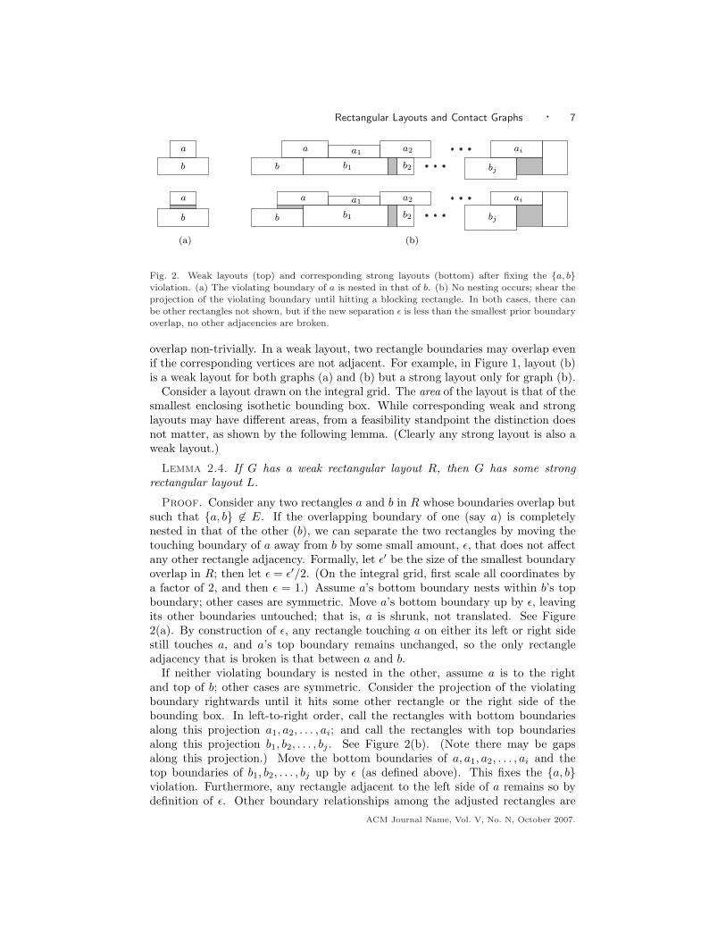
Fig. 2. Weak layouts (top) and corresponding strong layouts (bottom) after fixing the a, bviolation. (a) The violating boundary of a is nested in that of b. (b) No nesting occurs; shear theprojection of the violating boundary until hitting a blocking rectangle. In both cases, there canbe other rectangles not shown, but if the new separation ε is less than the smallest prior boundaryoverlap, no other adjacencies are broken.

overlap non-trivially. In a weak layout, two rectangle boundaries may overlap evenif the corresponding vertices are not adjacent. For example, in Figure 1, layout (b)is a weak layout for both graphs (a) and (b) but a strong layout only for graph (b).

Consider a layout drawn on the integral grid. The area of the layout is that of thesmallest enclosing isothetic bounding box. While corresponding weak and stronglayouts may have different areas, from a feasibility standpoint the distinction doesnot matter, as shown by the following lemma. (Clearly any strong layout is also aweak layout.)

Lemma 2.4. If G has a weak rectangular layout R, then G has some strongrectangular layout L.

Proof. Consider any two rectangles a and b in R whose boundaries overlap butsuch that a, b 6∈ E. If the overlapping boundary of one (say a) is completelynested in that of the other (b), we can separate the two rectangles by moving thetouching boundary of a away from b by some small amount, ε, that does not affectany other rectangle adjacency. Formally, let ε′ be the size of the smallest boundaryoverlap in R; then let ε = ε′/2. (On the integral grid, first scale all coordinates bya factor of 2, and then ε = 1.) Assume a’s bottom boundary nests within b’s topboundary; other cases are symmetric. Move a’s bottom boundary up by ε, leavingits other boundaries untouched; that is, a is shrunk, not translated. See Figure2(a). By construction of ε, any rectangle touching a on either its left or right sidestill touches a, and a’s top boundary remains unchanged, so the only rectangleadjacency that is broken is that between a and b.

If neither violating boundary is nested in the other, assume a is to the rightand top of b; other cases are symmetric. Consider the projection of the violatingboundary rightwards until it hits some other rectangle or the right side of thebounding box. In left-to-right order, call the rectangles with bottom boundariesalong this projection a1, a2, . . . , ai; and call the rectangles with top boundariesalong this projection b1, b2, . . . , bj . See Figure 2(b). (Note there may be gapsalong this projection.) Move the bottom boundaries of a, a1, a2, . . . , ai and thetop boundaries of b1, b2, . . . , bj up by ε (as defined above). This fixes the a, bviolation. Furthermore, any rectangle adjacent to the left side of a remains so bydefinition of ε. Other boundary relationships among the adjusted rectangles are



preserved, and no other boundaries are affected.Repeating this process to fix each violation produces L.

Lemma 2.4 addresses feasibility of rectangle layouts only; the expansion in areafrom the transformation might be exponential. Later we give procedures to drawstrong layouts directly with better areas.

In the sequel, we will use the term layout to refer to strong layouts. Furthermore,the assumption that no two rectangles meet trivially at a corner is without loss ofgenerality. Say rectangles a and b so meet. We can perturb the boundaries bysome small amount to make the boundary overlap non-trivial. The layout becomesweak if it was not already. Lemma 2.4 shows that it can be made strong with onlynon-trivial boundary overlaps.

3. CHARACTERIZING RECTANGULAR LAYOUTS

3.1 Background

Thomassen [1986, Thm. 2.1] characterizes graphs that admit rectangular layouts(which he calls strict rectangle graphs) as precisely the class of proper subgraphs of4-connected planar triangulations. Together with earlier work [Thomassen 1984],his work yields a polynomial-time algorithm for testing a graph G to see if it admitsa rectangular layout and, if so, constructing such a layout. He does not analyze thealgorithm precisely for running time, however, nor does he bound the layout areaat all, two criteria that concern us.

Thomassen’s work rests critically on earlier work by Ungar [1953]. Ungar definesa saturated plane map to be a finite set of non-overlapping regions that partitionsthe plane and satisfies the following conditions.

(1) Precisely one region is infinite.(2) At most three regions meet in any point.(3) Every region is simply connected.(4) The union of any two adjacent regions is simply connected.(5) The intersection of any two regions is either a simple arc or is empty.

An n-ring is a set of n regions such that their union is multiply connected.1

Ungar [1953, Thm. A] shows that a saturated plane map that contains no 3-ringis isomorphic to a rectangular dissection. Ungar [1953, Thm. B] further impliesthat for any rectangular dissection R and any two adjacent rectangles a and bin R, there exists a rectangular dissection R′ isomorphic to R such that a′ (theregion in R′ corresponding to a in R) is the infinite region and b′ (the rectangle inR′ corresponding to b in R) has three or four whole sides fully exposed: i.e., notoverlapping any rectangle other than a′.

We prove the following “folklore” lemma in the Appendix.

Lemma 3.1. A graph G is planar, cubic, and cyclically 4-edge connected if andonly if G is a saturated plane map with no 3-ring.

Using Lemma 3.1, Thomassen [1986] rephrases Ungar’s Theorem A as follows.

1Connectivity in this definition and conditions 3–5 above is in the topological sense.



Lemma 3.2. Any cubic, cyclically 4-edge connected planar graph has a rectan-gular representation.

3.2 New Characterization

Kozminski and Kinnen [1985] define a 4-triangulation to be a 4-connected, pla-nar triangulated graph with at least 6 vertices, at least one of which has degree 4.Kozminski and Kinnen [1985, Thm. 1] prove that a cube with one face that is a rect-angular dissection is dual to a planar graph G if and only if G is a 4-triangulation.Kozminski and Kinnen [1985, Thm. 2] also prove that a planar graph G with allfaces triangular except the outside has a rectangular dual if and only if G canbe obtained from some 4-triangulation H by the deletion of some degree-4 vertexand all its neighbors. We use the following somewhat weaker result to design analgorithm for constructing rectangular layouts.

Theorem 3.3. If a planar graph G can be derived from some 4-connected planartriangulation H by the removal of some vertex and its incident edges, then G hasa rectangular dual.

Proof. Let H be any 4-connected planar triangulation and v any vertex of H.By Lemma 2.2, H∗ is planar, cubic, and cyclically 4-edge connected, so by Lemma3.1, H∗ yields a saturated plane map M with no 3-ring. Ungar [1953, Thm. B]implies that an isomorphic map M ′ exists with the external face corresponding tov. M ′ is thus a rectangular dual for the graph derived from H by removing v andits incident edges.

The benefit of Theorem 3.3 is that it gives a sufficient condition for rectangularduality in terms of 4-connected triangulations rather than Kozminski and Kinnen’s[1985] 4-triangulations. This yields (in Section 4) a simple augmentation procedurefor constructing rectangular layouts based on the following alternative characteri-zation of graphs admitting rectangular layouts.

Theorem 3.4. A planar graph G is a proper subgraph of a 4-connected planartriangulation if and only if G has an embedding with no filled triangles.

Proof. (=⇒) Let G′ be a 4-connected planar triangulation. Let G be the resultof removing any one edge or vertex (and its incident edges) from G′. By Lemma2.1, G′, and therefore G, has no separating triangle. We claim that any embeddingE of G has a non-triangular face or that G is itself just a 3-vertex cycle. To provethe claim, consider an arbitrary embedding E ′ of G′. Removing a single edge fromE ′ yields an embedding E (of G) with a non-triangular face. If removing a vertex vfrom E ′ yields an embedding E with no non-triangular face, then E itself must bea simple triangle; otherwise, the triangular face of E to which v was adjacent is aseparating triangle in E ′, which by assumption cannot exist. This proves the claim.

If G is a 3-vertex cycle, we are done; otherwise, by stereographic projection,we can assume that its external face is non-triangular. Because any filled triangleis either a separating triangle or the external face, it follows that E has no filledtriangles, and therefore any proper subgraph of G also has an embedding with nofilled triangles.

(⇐=) Now let G be a planar graph, and let E be some embedding of G withno filled triangles. Assume without loss of generality that G has at least one non-



triangular face. Otherwise, G itself is a triangulation, and the assumption that Ehas no filled triangles implies that G is simply a 3-vertex cycle. We will show how toform by vertex augmentation a proper supergraph G′ of G such that G′ is a planartriangulation with no separating triangles and hence by Lemma 2.1 is 4-connected.

First, we may assume that G is biconnected. Otherwise, we adapt a procedureattributed to Read [1987]. Consider any articulation vertex v, and let u and w beconsecutive neighbors of v in separate biconnected components. Add new vertexz and edges z, u and z, w. Iterating for every articulation point biconnects Gwithout adding separating triangles. Any face in the updated embedding E is thenbounded by a simple cycle, and the following procedure is well defined.

Consider any non-triangular facial cycle F in E . Define a chord of F to be anon-facial edge connecting two vertices of F . Consider any chord x, y of F , andlet u and v be the neighbors of x on F . There can be no edge u, v in G, for suchan edge would violate planarity. Therefore embedding a new vertex ν(x) insideF and adding edges ν(x), u, ν(x), x, and ν(x), v cannot create a separatingtriangle. Let F ′ be the new facial cycle defined by replacing the path (u, x, v) inF by (u, ν(x), v), and iterate until F ′ has no incident chords. Then, adding a finalnew vertex ν(F ) with edges to each vertex on F ′ completes the triangulation ofthe original face F without creating separating triangles or modifying other faces.Iterating for all non-triangular facial cycles completes the process, yielding a planartriangulation G′ with no additional separating triangles.

Therefore, any separating triangle T in G′ must have originally existed in G.Because E had no filled triangles, T must have been embedded as a (triangular)face of E . T remains a face in G′, however, and because G′ is a triangulation, theremoval of any face cannot disconnect G′, thereby contradicting the existence ofT .

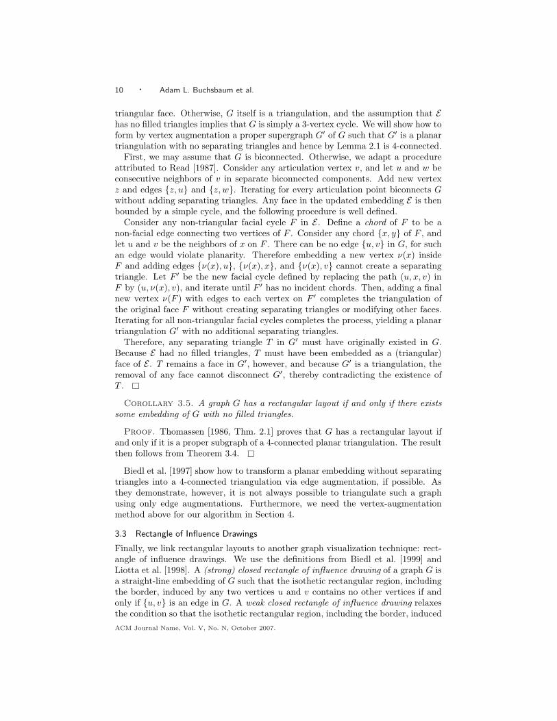
Corollary 3.5. A graph G has a rectangular layout if and only if there existssome embedding of G with no filled triangles.

Proof. Thomassen [1986, Thm. 2.1] proves that G has a rectangular layout ifand only if it is a proper subgraph of a 4-connected planar triangulation. The resultthen follows from Theorem 3.4.

Biedl et al. [1997] show how to transform a planar embedding without separatingtriangles into a 4-connected triangulation via edge augmentation, if possible. Asthey demonstrate, however, it is not always possible to triangulate such a graphusing only edge augmentations. Furthermore, we need the vertex-augmentationmethod above for our algorithm in Section 4.

3.3 Rectangle of Influence Drawings

Finally, we link rectangular layouts to another graph visualization technique: rect-angle of influence drawings. We use the definitions from Biedl et al. [1999] andLiotta et al. [1998]. A (strong) closed rectangle of influence drawing of a graph G isa straight-line embedding of G such that the isothetic rectangular region, includingthe border, induced by any two vertices u and v contains no other vertices if andonly if u, v is an edge in G. A weak closed rectangle of influence drawing relaxesthe condition so that the isothetic rectangular region, including the border, inducedACM Journal Name, Vol. V, No. N, October 2007.


by any two vertices u and v contains no other vertices if u, v is an edge in G.A (strong or weak) open rectangle of influence drawing is one in which all the iso-thetic rectangular interiors obey the respective emptyness constraints; the interiorsof degenerate rectangles are defined to be those of the induced line segments. Thesedrawings are also planar if no two edges cross.

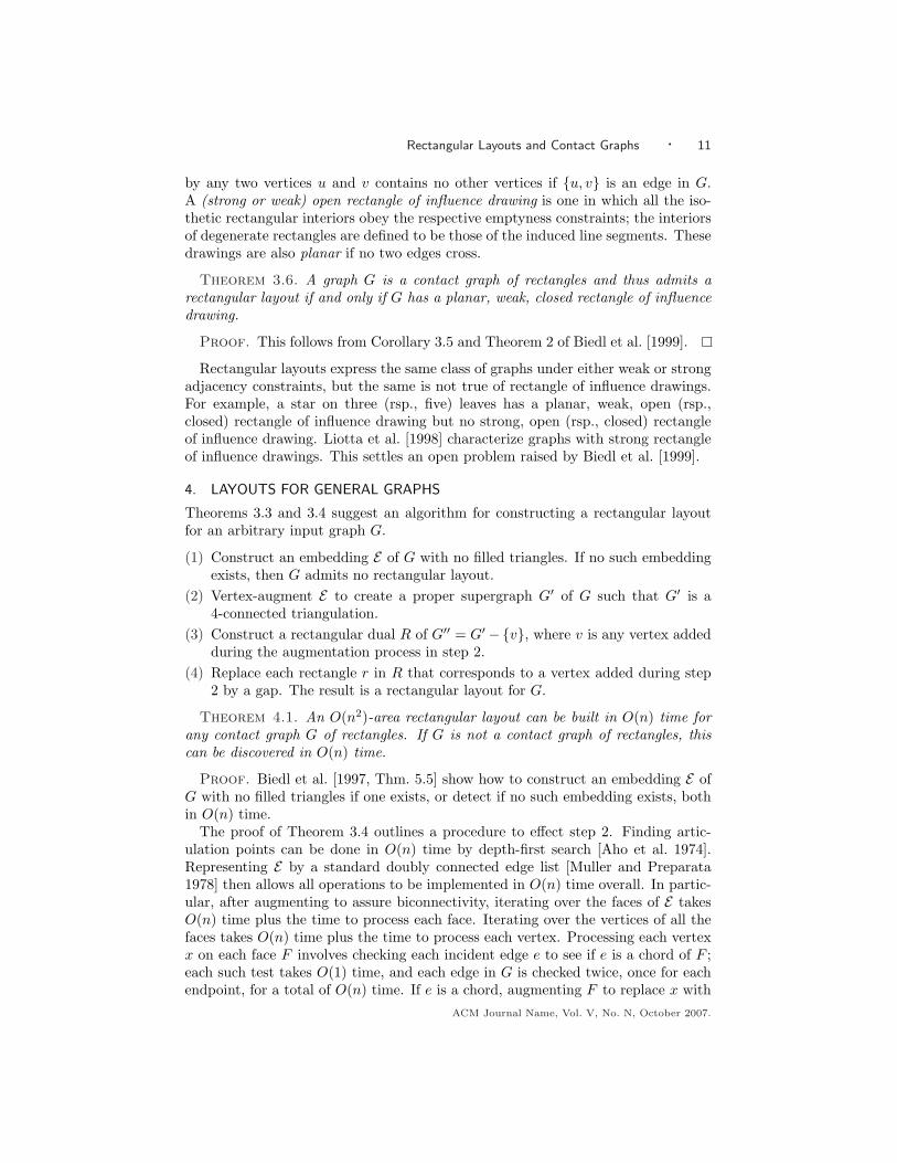
Theorem 3.6. A graph G is a contact graph of rectangles and thus admits arectangular layout if and only if G has a planar, weak, closed rectangle of influencedrawing.

Proof. This follows from Corollary 3.5 and Theorem 2 of Biedl et al. [1999].

Rectangular layouts express the same class of graphs under either weak or strongadjacency constraints, but the same is not true of rectangle of influence drawings.For example, a star on three (rsp., five) leaves has a planar, weak, open (rsp.,closed) rectangle of influence drawing but no strong, open (rsp., closed) rectangleof influence drawing. Liotta et al. [1998] characterize graphs with strong rectangleof influence drawings. This settles an open problem raised by Biedl et al. [1999].

4. LAYOUTS FOR GENERAL GRAPHS

Theorems 3.3 and 3.4 suggest an algorithm for constructing a rectangular layoutfor an arbitrary input graph G.

(1) Construct an embedding E of G with no filled triangles. If no such embeddingexists, then G admits no rectangular layout.

(2) Vertex-augment E to create a proper supergraph G′ of G such that G′ is a4-connected triangulation.

(3) Construct a rectangular dual R of G′′ = G′−v, where v is any vertex addedduring the augmentation process in step 2.

(4) Replace each rectangle r in R that corresponds to a vertex added during step2 by a gap. The result is a rectangular layout for G.

Theorem 4.1. An O(n2)-area rectangular layout can be built in O(n) time forany contact graph G of rectangles. If G is not a contact graph of rectangles, thiscan be discovered in O(n) time.

Proof. Biedl et al. [1997, Thm. 5.5] show how to construct an embedding E ofG with no filled triangles if one exists, or detect if no such embedding exists, bothin O(n) time.

The proof of Theorem 3.4 outlines a procedure to effect step 2. Finding artic-ulation points can be done in O(n) time by depth-first search [Aho et al. 1974].Representing E by a standard doubly connected edge list [Muller and Preparata1978] then allows all operations to be implemented in O(n) time overall. In partic-ular, after augmenting to assure biconnectivity, iterating over the faces of E takesO(n) time plus the time to process each face. Iterating over the vertices of all thefaces takes O(n) time plus the time to process each vertex. Processing each vertexx on each face F involves checking each incident edge e to see if e is a chord of F ;each such test takes O(1) time, and each edge in G is checked twice, once for eachendpoint, for a total of O(n) time. If e is a chord, augmenting F to replace x with



ν(x) also takes O(1) time. Adding vertex ν(F ) takes time linear in the number ofvertices on F ; over all faces this is O(n) time. In all, step 2 can be done in O(n)time, yielding graph G′′ ⊇ G with O(n) vertices.

Theorem 3.3 asserts that G′′ has a rectangular dual. He [1993] shows how toconstruct an O(n2)-area rectangular dual of G′′ in O(n) time.2 During the con-struction, we simply indicate that any rectangle corresponding to a vertex in G′′−Gshould instead be rendered as a gap. Since each edge in G′′ − G is incident to atleast one vertex in G′′ −G, the result is a rectangular layout for G.

4.1 General Lower Bound

A trivial, worst-case lower bound for graphs is

max

n,

∑

v∈V

⌈deg(v)

4

⌉,∑

v∈V

⌈deg(v)− 2

2

⌉,

where deg(v) is the degree of vertex v. The second term comes from the fact thateach vertex v is represented by a rectangle, which has 4 sides; the area of thatrectangle must therefore be at least ddeg(v)

4 e to accommodate all the adjacencies.This is tight in general: consider the infinite grid, in which each vertex has degree4 and the area required is |V |. The third term generalizes this argument. Theperimeter of v’s rectangle must be at least deg(v) units. If the sides of the rectanglehave lengths a and b, then minimizing ab subject to a + b ≥ d/2 yields that ab ≥ddeg(v)−2

2 e.To show a worst-case lower bound that matches our upper bound, first define

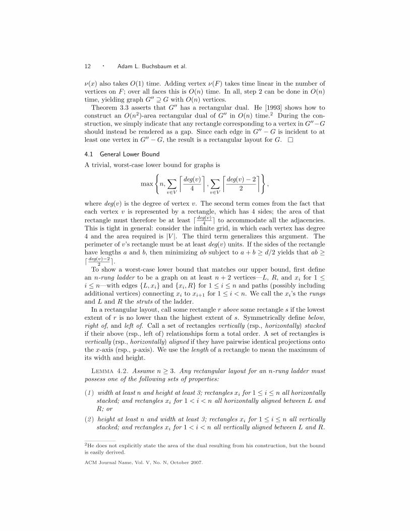
an n-rung ladder to be a graph on at least n + 2 vertices—L, R, and xi for 1 ≤i ≤ n—with edges L, xi and xi, R for 1 ≤ i ≤ n and paths (possibly includingadditional vertices) connecting xi to xi+1 for 1 ≤ i < n. We call the xi’s the rungsand L and R the struts of the ladder.

In a rectangular layout, call some rectangle r above some rectangle s if the lowestextent of r is no lower than the highest extent of s. Symmetrically define below,right of, and left of. Call a set of rectangles vertically (rsp., horizontally) stackedif their above (rsp., left of) relationships form a total order. A set of rectangles isvertically (rsp., horizontally) aligned if they have pairwise identical projections ontothe x-axis (rsp., y-axis). We use the length of a rectangle to mean the maximum ofits width and height.

Lemma 4.2. Assume n ≥ 3. Any rectangular layout for an n-rung ladder mustpossess one of the following sets of properties:

(1 ) width at least n and height at least 3; rectangles xi for 1 ≤ i ≤ n all horizontallystacked; and rectangles xi for 1 < i < n all horizontally aligned between L andR; or

(2 ) height at least n and width at least 3; rectangles xi for 1 ≤ i ≤ n all verticallystacked; and rectangles xi for 1 < i < n all vertically aligned between L and R.

2He does not explicitly state the area of the dual resulting from his construction, but the boundis easily derived.



x1 x2 x3 x4. . . . . . x5

R

L

L

R

x5x1 x3

x2 x4 . . . . . .

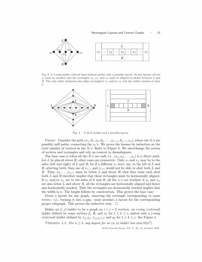
Fig. 3. A 5-rung ladder (dotted lines indicate paths) and a possible layout. In any layout, all thexi must be stacked, and the rectangles x2, x3, and x4 must be aligned as shown between L andR. The only other variations also align rectangle(s) x1 and/or x5, but the width remains at least5.

L R

T

B

T

L R

B

Fig. 4. A (6, 6)-ladder and a possible layout.

Proof. Consider the path (x1, S1, x2, S2, . . . , xn−1, Sn−1, xn), where the Si’s arepossibly null paths, connecting the xi’s. We prove the lemma by induction on thetotal number of vertices in the Si’s. Refer to Figure 3. We interchange the notionof vertices and rectangles and rely on context to disambiguate.

The base case is when all the Si’s are null; i.e., (x1, x2, . . . , xn) is a direct path.Let L be placed above R; other cases are symmetric. Only x1 and xn may be to thesides (left and right) of L and R, for if a different xi were, say, to the left of L andR, abutting both, then one of xi−1 and xi+1 would not be able to abut both L andR. Thus, x2, . . . , xn−1 must be below L and above R; that they must each abutboth L and R therefore implies that these rectangles must be horizontally aligned.If x1 and/or xn are to the sides of L and R, all the xi’s are stacked; if x1 and xn

are also below L and above R, all the rectangles are horizontally aligned and hencealso horizontally stacked. That the rectangles are horizontally stacked implies thatthe width is n. The height follows by construction. This proves the base case.

Given a layout for any graph, removing the rectangle corresponding to somevertex—i.e., turning it into a gap—must produce a layout for the correspondingproper subgraph. This proves the inductive step.

Define an (i, j)-ladder to be a graph on i + j + 2 vertices: an i-rung (external)ladder defined by some vertices L, R, and xk for 1 ≤ k ≤ i, united with a j-rung(internal) ladder defined by xbi/2c, xbi/2c+1, and yk for 1 ≤ k ≤ j. See Figure 4.

Theorem 4.3. For n ≥ 4, any layout for an (n, n)-ladder has area Ω(n2).ACM Journal Name, Vol. V, No. N, October 2007.


Proof. Lemma 4.2 applied to the external ladder shows that the height (or,rsp., width) of any layout is at least n and that the rectangles xbn/2c and xbn/2c+1

are vertically (or, rsp., horizontally) aligned between L and R. Say the height isn; the other case is symmetric. Then Lemma 4.2 shows that the width induced bythe internal ladder is at least n. The theorem follows.

5. LAYOUTS FOR TREES

We present an algorithm that constructs O(n log n)-area rectangular layouts fortrees. We then show a matching worst-case lower bound. There do exist trees withbetter layouts, however, and we constructively show an infinite class of trees thathave O(n)-area layouts. As with general graphs, this leaves open the problem ofdevising better approximation algorithms for trees.

5.1 General Algorithm

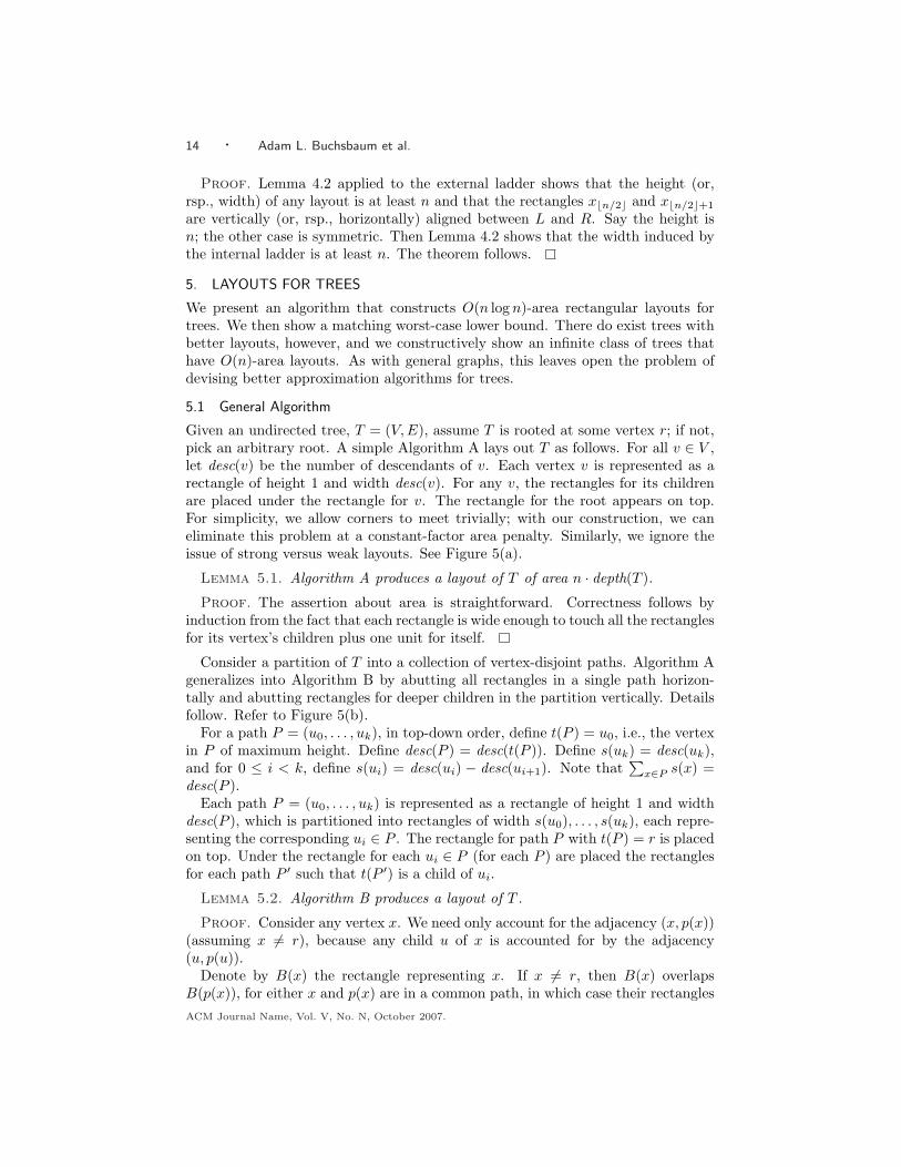
Given an undirected tree, T = (V, E), assume T is rooted at some vertex r; if not,pick an arbitrary root. A simple Algorithm A lays out T as follows. For all v ∈ V ,let desc(v) be the number of descendants of v. Each vertex v is represented as arectangle of height 1 and width desc(v). For any v, the rectangles for its childrenare placed under the rectangle for v. The rectangle for the root appears on top.For simplicity, we allow corners to meet trivially; with our construction, we caneliminate this problem at a constant-factor area penalty. Similarly, we ignore theissue of strong versus weak layouts. See Figure 5(a).

Lemma 5.1. Algorithm A produces a layout of T of area n · depth(T ).

Proof. The assertion about area is straightforward. Correctness follows byinduction from the fact that each rectangle is wide enough to touch all the rectanglesfor its vertex’s children plus one unit for itself.

Consider a partition of T into a collection of vertex-disjoint paths. Algorithm Ageneralizes into Algorithm B by abutting all rectangles in a single path horizon-tally and abutting rectangles for deeper children in the partition vertically. Detailsfollow. Refer to Figure 5(b).

For a path P = (u0, . . . , uk), in top-down order, define t(P ) = u0, i.e., the vertexin P of maximum height. Define desc(P ) = desc(t(P )). Define s(uk) = desc(uk),and for 0 ≤ i < k, define s(ui) = desc(ui) − desc(ui+1). Note that

∑x∈P s(x) =

desc(P ).Each path P = (u0, . . . , uk) is represented as a rectangle of height 1 and width

desc(P ), which is partitioned into rectangles of width s(u0), . . . , s(uk), each repre-senting the corresponding ui ∈ P . The rectangle for path P with t(P ) = r is placedon top. Under the rectangle for each ui ∈ P (for each P ) are placed the rectanglesfor each path P ′ such that t(P ′) is a child of ui.

Lemma 5.2. Algorithm B produces a layout of T .

Proof. Consider any vertex x. We need only account for the adjacency (x, p(x))(assuming x 6= r), because any child u of x is accounted for by the adjacency(u, p(u)).

Denote by B(x) the rectangle representing x. If x 6= r, then B(x) overlapsB(p(x)), for either x and p(x) are in a common path, in which case their rectanglesACM Journal Name, Vol. V, No. N, October 2007.


c d

a

m n

ig h

b

j k l

fe

b f l

kje

c g h m

a d i n

(a)

a

b c d

e g i

j k l

f h

m n(b)

a

b c d

e g i

j k l

f h

m n

Fig. 5. (a) A tree and the result of applying Algorithm A. The width of each rectangle is thenumber of descendants of the corresponding vertex; e.g., the width of f is 4, and the width ofd is 6. (b) A partition of the tree into paths—uncircled nodes form singleton paths—and theapplication of Algorithm B to the partition.

share a vertical side, or else B(x) is layed out underneath B(p(x)). The constructionassures that B(p(x)) is wide enough in this latter case.

Consider the compressed tree C(T ), formed by compressing each path P into asuper-vertex, with edges to each super-vertex P ′ such that t(P ′) is a child of somex ∈ P .

Lemma 5.3. Algorithm B produces a layout of T of area n · depth(C(T )).

Proof. Algorithm B produces a one-unit high collection of rectangles for eachdistinct depth in C(T ). Each such collection is of width no more than n (the totalnumber of descendants of the paths at that depth).

We use the heavy-path partition of T , as defined by Harel and Tarjan [1984] andlater used by Gabow [1990].3 Call tree edge (v, p(v)) light if 2 ·desc(v) ≤ desc(p(v)),and heavy otherwise. Since a heavy edge must carry more than half the descendantsof a vertex, each vertex can have at most one heavy edge to a child, and thereforedeletion of the light edges produces a collection of vertex-disjoint heavy paths. (A

3Tarjan [1979] originally introduced heavy-path partitions, but defined in different terms; Schieberand Vishkin [1988] later used yet another variant.



vertex with no incident heavy edges becomes a singleton, called a trivial heavypath.)

Theorem 5.4. Algorithm B applied to the heavy-path partition of T produces alayout of area O(n log n) in O(n) time.

Proof. The compressed tree, C(T ), is constructed by contracting each heavypath in T into a single super-vertex. Each tree edge in C(T ) corresponds to a lightedge of T . Since there are O(log n) light edges on the path from any vertex tothe root of T , C(T ) has depth O(log n). The area bound follows from Lemmas 5.2and 5.3. C(T ) can be built in O(n) time after a depth-first search; the rest of thealgorithm performs O(1) work per vertex.

5.2 General Lower Bound

We show there exists an infinite family of trees that require Ω(n log n) area for anylayout. First we show that any layout of a binary tree has Ω(log n) length in eachdimension.

We define the notion of paths in layouts. A path in layout L is a sequence(r1, . . . , r`) of rectangles in L such that for each 1 ≤ i < `, the boundaries of ri

and ri+1 overlap. A path in a strong layout thus corresponds to a path in theunderlying graph. A vertical extremal path of L is a path that touches both the topand bottom of L’s bounding box B; similarly, define a horizontal extremal path totouch the left and right sides of B. An extremal path that touches opposite cornersof B is both vertical and horizontal. By definition, every layout has at least onevertical and at least one horizontal extremal path, possibly identical.

Consider graph G with some layout L and some subgraph G′. L contains a sub-layout L′ for G′. Any extremal path in L′ induces a path in L. Two sub-layoutsare disjoint if their induced subgraphs are disjoint. Extremal paths for disjointsub-layouts may not cross in L, for this would imply two non-disjoint rectangles, afact codified as follows.

Fact 5.5. Consider graph G, some layout L of G, and any two disjoint, con-nected subgraphs G1 and G2 of G. Extremal paths for the corresponding sub-layoutsL1 and L2 may not cross in L.

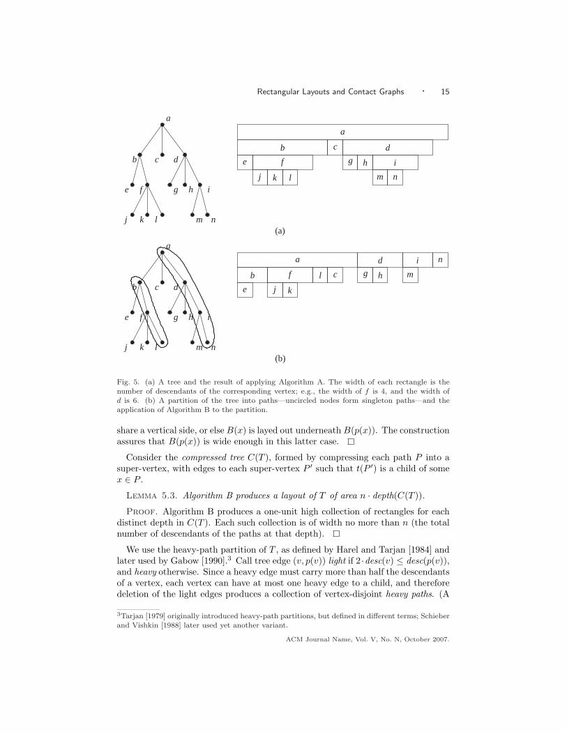
Lemma 5.6. Let G1 and G2 have minimal area layouts with length at least d ineach dimension. Let G contain both G1 and G2 as subgraphs. Then any layout Lof G has length at least d + 1 in at least one dimension.

Proof. Since L contains sub-layouts L1 and L2 for G1 and G2, rsp., by assump-tion L has length at least d in both dimensions. If L has width and height both d,then any horizontal extremal path for L1 must cross any vertical extremal path forL2, contradicting Fact 5.5. Thus, L must have width or height at least d + 1. (SeeFigure 6.)

Lemma 5.7. Let G1 and G2 be graphs such that all their layouts have length atleast d in each dimension. Let G be formed by adding a new vertex r, adjacentto one vertex in each of G1 and G2. Then in any layout L of G with length d insome dimension, r cannot be incident to a length-d side of the bounding box of L.ACM Journal Name, Vol. V, No. N, October 2007.


(d)(c)(b)(a)

Fig. 6. Bounding boxes and extremal paths for various layouts. (a) Layout L1 for G1; (b) LayoutL2 for G2; each of size d-by-d. (c) Impossible d-by-d layout for G containing G1 and G2 assubgraphs; any corresponding extremal paths would have to cross. (d) d-by-(d + 1) layout for G.The extremal path for L1 is dotted, and that for L2 is dashed. By extending G in one dimension,the extremal paths need not cross.

Furthermore there exist extremal paths in the length-d dimension to either side ofr.

Proof. (Refer to Figure 7(a).) Assume to the contrary that L has width d and ris adjacent to the bottom (sym., top) of L; the argument for height d is symmetric.L induces layouts L1 of G1 and L2 of G2, each by assumption with length at leastd in each dimension d. Let r be adjacent to a rectangle ` of L1 (sym., L2). Thenthere must be a path P from ` that intersects a horizontal extremal path P1 of bothL1 and L. The union of P and one side of this extremal path forms a closed curvewith the bounding box that contains r.

Now consider a horizontal extremal path P2 of L2, which is also a horizontalextremal path of L. There must be a path P ′ in L2 connecting P2 to r. P2 cannotintersect the closed curve defined above without creating non-disjoint rectangles;thus P2 is above P1. But then by the Jordan curve theorem [Munkres 1999, Section8-13], P ′ itself must cross the curve to reach P2, which again would create non-disjoint rectangles.

If r is above P2, a similar contradiction holds. Thus, r must be between P1 andP2.

Define Ti to be a complete binary tree on 2i leaves.

Lemma 5.8. Any layout for Ti has length at least bi/2c in each dimension.

Proof. The theorem is true for i = 0 and i = 1. Assuming it is true up to i−1,we prove it by induction for i ≥ 2. Denote by r the root of Ti and by u and v theroots of the Ti−1’s rooted at the children of r. By induction, each Ti−2 rooted atchildren of u and v has length at least

⌊i−22

⌋in each dimension. By Lemma 5.6

therefore, the layouts for the Ti−1 subtrees rooted at u and v each have at least onedimension of length

⌊i−22

⌋+ 1 = bi/2c. If either sub-layout has both dimensions

this large, we are done. If one sub-layout has width bi/2c and the other heightbi/2c, we are similarly done.

Therefore, assume the sub-layouts for both Ti−1’s have height⌊

i−22

⌋. (Symmet-

rically argue if both widths are this small.) Also assume that in the layout for Ti, ris not placed on top of the two sub-layouts, or the height grows by the required oneunit. By Lemma 5.7, neither u nor v may be adjacent to the left or right side of



P1

P2

`r

P

(a)

u

v

(b)

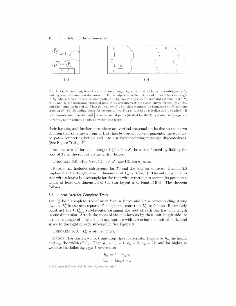
Fig. 7. (a) A bounding box of width d containing a layout L that includes two sub-layouts L1

and L2, each of minimum dimension d. If r is adjacent to the bottom of L, let ` be a rectanglein L1 adjacent to r. There is some path P in L1 connecting ` to a horizontal extremal path P1

of L1 and L. No horizontal extremal path of L2 can intersect the closed curves formed by P , P1,and the bounding box of L. Thus P2 is above P1, but then r cannot be connected to P2 withoutcrossing P1. (b) Bounding boxes for layouts of two Ti−1’s, rooted at u (solid) and v (dashed). If

both layouts are of heightj

i−22

k, then extremal paths (dashed for the Ti−1 rooted at v) separate

u from v, and r cannot be placed within this height.

their layouts, and furthermore, there are vertical extremal paths due to their ownchildren that separate u from v. But then by Jordan curve arguments, there cannotbe paths connecting both u and v to r without violating rectangle disjointedness.(See Figure 7(b).)

Assume n = 2k for some integer k ≥ 1. Let Sn be a tree formed by linking theroot of Tk to the root of a star with n leaves.

Theorem 5.9. Any layout Ln for Sn has Ω(n log n) area.

Proof. Ln includes sub-layouts for Tk and the star on n leaves. Lemma 5.8implies that the length of each dimension of Ln is Ω(log n). The only layout for astar with n leaves is a rectangle for the root with n rectangles around its perimeter.Thus, at least one dimension of the star layout is of length Ω(n). The theoremfollows.

5.3 Linear Area for Complete Trees

Let T kn be a complete tree of arity k on n leaves and Lk

n a corresponding stronglayout. Lk

1 is the unit square. For higher n, construct Lkn as follows. Recursively

construct the k Lkn/k sub-layouts, assuming the root of each one has unit length

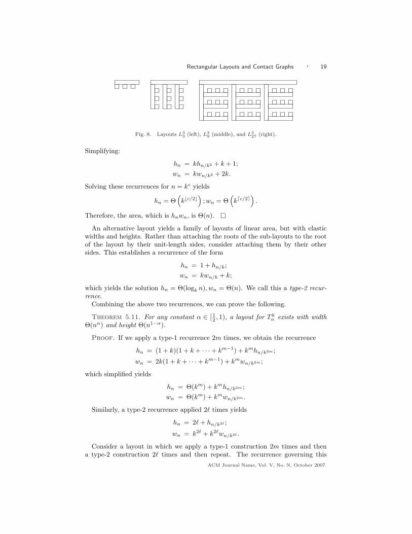
in one dimension. Attach the roots of the sub-layouts by their unit-length sides toa root rectangle of height 1 and appropriate width, leaving one unit of horizontalspace to the right of each sub-layout. See Figure 8.

Theorem 5.10. Lkn is of area O(n).

Proof. For clarity, we fix k and drop the superscripts. Denote by hn the heightand wn the width of Ln. Then h1 = w1 = 1; hk = 2, wk = 2k; and for higher n,we have the following type-1 recurrence:

hn = 1 + wn/k;wn = khn/k + k.



Fig. 8. Layouts L33 (left), L3

9 (middle), and L327 (right).

Simplifying:

hn = khn/k2 + k + 1;wn = kwn/k2 + 2k.

Solving these recurrences for n = kc yields

hn = Θ(kbc/2c

); wn = Θ

(kdc/2e

).

Therefore, the area, which is hnwn, is Θ(n).

An alternative layout yields a family of layouts of linear area, but with elasticwidths and heights. Rather than attaching the roots of the sub-layouts to the rootof the layout by their unit-length sides, consider attaching them by their othersides. This establishes a recurrence of the form

hn = 1 + hn/k;wn = kwn/k + k;

which yields the solution hn = Θ(logk n), wn = Θ(n). We call this a type-2 recur-rence.

Combining the above two recurrences, we can prove the following.

Theorem 5.11. For any constant α ∈ [ 12 , 1), a layout for T kn exists with width

Θ(nα) and height Θ(n1−α).

Proof. If we apply a type-1 recurrence 2m times, we obtain the recurrence

hn = (1 + k)(1 + k + · · ·+ km−1) + kmhn/k2m ;

wn = 2k(1 + k + · · ·+ km−1) + kmwn/k2m ;

which simplified yields

hn = Θ(km) + kmhn/k2m ;wn = Θ(km) + kmwn/k2m .

Similarly, a type-2 recurrence applied 2` times yields

hn = 2` + hn/k2` ;

wn = k2` + k2`wn/k2` .

Consider a layout in which we apply a type-1 construction 2m times and thena type-2 construction 2` times and then repeat. The recurrence governing this



construction is given by a combination of the above two recurrences:

hn = Θ(km) + km(2` + hn/k(2`+2m));

wn = Θ(km) + km(k2` + k2`wn/k(2`+2m));

which simplifies to

hn = Θ(km`) + kmhn/k(2`+2m) ;

wn = Θ(km+2`) + km+2`wn/k(2`+2m) .

Solving these recurrences and setting α = 1 − m/(2m + 2`), we get hn =Θ(n1−α(1 + `)) and wn = Θ(nα). For any 1/2 ≤ α < 1 we can find constants` and m that satisfy this equation.

6. AREA OPTIMALITY

6.1 NP-Hardness of Generating Optimal Layouts

Recall the problem of numerical matching with target sums [Garey and Johnson1979]. Given are disjoint sets X and Y , each of m elements, a size s(a) ∈ Z+

for each a ∈ X ∪ Y , and a target vector B = (B1, . . . , Bm) with each Bi ∈ Z+.The problem is to determine if X ∪ Y can be partitioned into m disjoint setsA1, . . . , Am, each containing exactly one element from each of X and Y , such thatfor 1 ≤ i ≤ m,

∑a∈Ai

s(a) = Bi. The problem is strongly NP-hard in general.Consider some instance I of numerical matching with target sums. Assume withoutloss of generality that

∑

x∈X

s(x) +∑

y∈Y

s(y) =m∑

i=1

Bi, (1)

or else I has no solution. We will construct a graph G(I) that has an optimallayout of certain dimensions if and only if I has a solution.

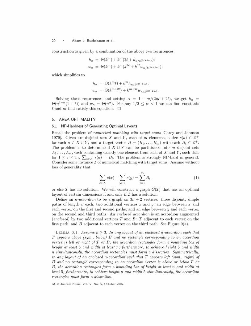
Define an n-accordion to be a graph on 3n + 2 vertices: three disjoint, simplepaths of length n each; two additional vertices x and y; an edge between x andeach vertex on the first and second paths; and an edge between y and each vertexon the second and third paths. An enclosed accordion is an accordion augmented(enclosed) by two additional vertices T and B: T adjacent to each vertex on thefirst path, and B adjacent to each vertex on the third path. See Figure 9(a).

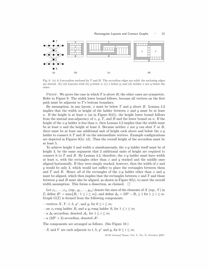
Lemma 6.1. Assume n ≥ 3. In any layout of an enclosed n-accordion such thatT appears above (sym., below) B and no rectangle corresponding to an accordionvertex is left or right of T or B, the accordion rectangles form a bounding box ofheight at least 5 and width at least n; furthermore, to achieve height 5 and widthn simultaneously, the accordion rectangles must form a dissection. Symmetrically,in any layout of an enclosed n-accordion such that T appears left (sym., right) ofB and no rectangle corresponding to an accordion vertex is above or below T orB, the accordion rectangles form a bounding box of height at least n and width atleast 5; furthermore, to achieve height n and width 5 simultaneously, the accordionrectangles must form a dissection.



x

y

B

T

x

y

B

T

x y

B

T

x

y

B

T

(a) (b) (c) (d)

Fig. 9. (a) A 5-accordion enclosed by T and B. The accordion edges are solid; the enclosing edgesare dotted. (b)–(d) Layouts with (b) y below x; (c) x below y; and (d) neither x nor y below theother.

Proof. We prove the case in which T is above B; the other cases are symmetric.Refer to Figure 9. The width lower bound follows, because all vertices on the firstpath must be adjacent to T ’s bottom boundary.

By assumption, in any layout, x must be below T and y above B. Lemma 4.2implies that the width or height of the ladder between x and y must be at leastn. If the height is at least n (as in Figure 9(d)), the height lower bound followsfrom the mutual non-adjacency of x, y, T , and B and the lower bound on n. If theheight of the x-y ladder is less than n, then Lemma 4.2 implies that the width mustbe at least n and the height at least 3. Because neither x nor y can abut T or B,there must be at least one additional unit of height each above and below the x-yladder to connect it T and B via the intermediate vertices. Example configurationsare depicted in Figures 9(b)–(d). Thus the overall height of the accordion must beat least 5.

To achieve height 5 and width n simultaneously, the x-y ladder itself must be ofheight 3, by the same argument that 2 additional units of height are required toconnect it to T and B. By Lemma 4.2, therefore, the x-y ladder must have widthat least n, with the rectangles other than x and y stacked and the middle onesaligned horizontally. If they were simply stacked, however, then the width of x andy would be only 3, which would not suffice to place the rectangles between themand T and B. Hence all of the rectangles of the x-y ladder other than x and ymust be aligned, which then implies that the rectangles between x and T and thosebetween y and B must also be aligned, as shown in Figure 9(b), to meet the overallwidth assumption. This forms a dissection, as claimed.

Let x1, . . . , xm (rsp., y1, . . . , ym) denote the sizes of the elements of X (rsp., Y ) inI; define B∗ = maxBi : 1 ≤ i ≤ m; and define ∆i = 2B∗−Bi ≥ 1 for 1 ≤ i ≤ m.Graph G(I) is formed from the following components.

—vertices X, Y , t, b, g∗, and gi for 0 ≤ i ≤ m;—an xi-rung ladder Ri and a yi-rung ladder Si for 1 ≤ i ≤ m;—a ∆i-accordion, denoted Ai, for 1 ≤ i ≤ m;—a (2B∗ + 2)-accordion, denoted A∗.The components are arranged as follows. (See Figure 10.)

—X and Y are each adjacent to t, b, g∗ and gi for 0 ≤ i ≤ m;ACM Journal Name, Vol. V, No. N, October 2007.


A1

Am

A∗Sm

R1

Rm

S1

X Y

t

b

g∗

gm

g0

g1

gm−1

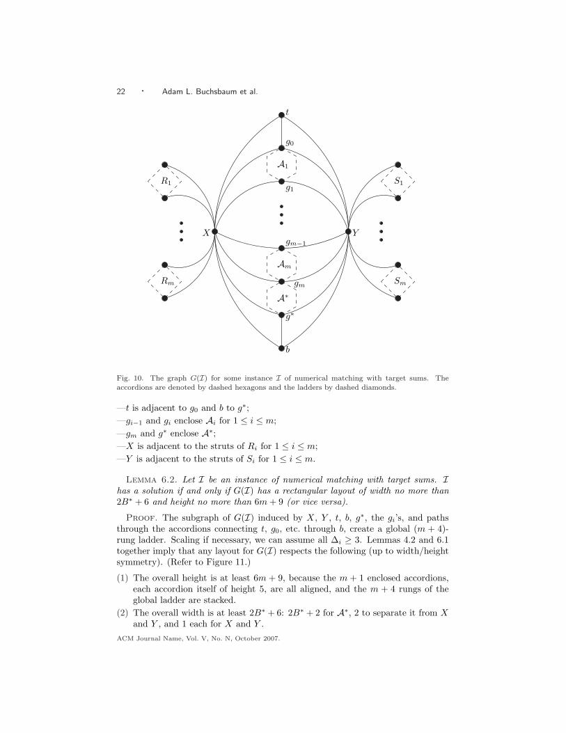
Fig. 10. The graph G(I) for some instance I of numerical matching with target sums. Theaccordions are denoted by dashed hexagons and the ladders by dashed diamonds.

—t is adjacent to g0 and b to g∗;—gi−1 and gi enclose Ai for 1 ≤ i ≤ m;—gm and g∗ enclose A∗;—X is adjacent to the struts of Ri for 1 ≤ i ≤ m;—Y is adjacent to the struts of Si for 1 ≤ i ≤ m.

Lemma 6.2. Let I be an instance of numerical matching with target sums. Ihas a solution if and only if G(I) has a rectangular layout of width no more than2B∗ + 6 and height no more than 6m + 9 (or vice versa).

Proof. The subgraph of G(I) induced by X, Y , t, b, g∗, the gi’s, and pathsthrough the accordions connecting t, g0, etc. through b, create a global (m + 4)-rung ladder. Scaling if necessary, we can assume all ∆i ≥ 3. Lemmas 4.2 and 6.1together imply that any layout for G(I) respects the following (up to width/heightsymmetry). (Refer to Figure 11.)

(1) The overall height is at least 6m + 9, because the m + 1 enclosed accordions,each accordion itself of height 5, are all aligned, and the m + 4 rungs of theglobal ladder are stacked.

(2) The overall width is at least 2B∗ + 6: 2B∗ + 2 for A∗, 2 to separate it from Xand Y , and 1 each for X and Y .



X

t

g0

g1

gm

g∗

b

A1

Y

A∗

gi−1

gi

AiX Y

(a) (b)

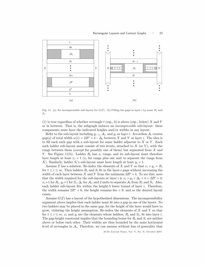
Fig. 11. (a) An incompressible sub-layout for G(I). (b) Filling the gaps in layer i by some Ri andSi.

(1) is true regardless of whether rectangle t (rsp., b) is above (rsp., below) X and Yor in between. That is, the subgraph induces an incompressible sub-layout: thesecomponents must have the indicated heights and/or widths in any layout.

Refer to the sub-layout including gi−1, Ai, and gi as layer i. Accordion Ai createsgap(s) of total width w(i) = 2B∗+ 4−∆i between X and Y at layer i. The idea isto fill each such gap with a sub-layout for some ladder adjacent to X or Y . Eachsuch ladder sub-layout must consist of two struts, attached to X (or Y ), with therungs between them (except for possibly one of them) but separated from X andY . See Figure 11(b). Ladder Ri has xi rungs, and its sub-layout must thereforehave length at least xi + 1 (xi for rungs plus one unit to separate the rungs fromX). Similarly, ladder Si’s sub-layout must have length at least yi + 1.

Assume I has a solution. Re-index the elements of X and Y so that xi +yi = Bi

for 1 ≤ i ≤ m. Then ladders Ri and Si fit in the layer-i gaps without increasing thewidth of each layer between X and Y from the minimum 2B∗+4. To see this, notethat the width required for the sub-layouts at layer i is xi + yi + ∆i + 4 = 2B∗+ 4:xi+1 for Ri, yi+1 for Si, ∆i forAi, and 2 units to separateAi from Ri and Si. Also,each ladder sub-layout fits within the height-5 lower bound of layer i. Therefore,the width remains 2B∗ + 6, the height remains 6m + 9, and so the desired layoutexists.

Assume G(I) has a layout of the hypothesized dimensions. The incompressibilityargument above implies that each ladder must fit into a gap in one of the layers. Notwo ladders may be placed in the same gap, for the height of the layer would have togrow, violating the height assumption. Re-index the elements of X and Y so thatfor 1 ≤ i ≤ m, xi and yi are the elements whose ladders, Ri and Si, fit into layer i.The gap-height constraint implies that the bounding boxes for Ri and Si are neitherabove or below each other. Their widths are thus bounded by the same horizontallevel of rectangles in Ai. Therefore, we can assume without loss of generality that



Ai is layed out as a dissection and thus by Lemma 6.1 in width ∆i. Because Ri

and Si fit into the layer-i gaps, it follows that xi + yi + 4 ≤ w(i) = 2B∗ + 4 −∆i

and hence xi + yi ≤ Bi. As this is true for all layers, Equation (1) implies thatxi + yi = Bi for all i, which gives a solution to I.

Theorem 6.3. Given a graph G and values W,H, A ∈ Z+, determining if G hasa (strong or weak) rectangular layout of (1) width no more than W and height nomore than H or (2) area no more than A is NP-complete.

Proof. Theorem 4.1 implies that the problem is in NP. Lemma 6.2 providesa P-time reduction showing NP-completeness, because the number of vertices andedges in G(I) is poly(m) and numerical matching with target sums is strongly NP-complete: for problem (1), set W = 2B∗+6 and H = 6m+9, and for problem (2),set A = (6m + 9)(2B∗ + 6). A similar reduction using height-3 accordions can beused for weak layouts.

Corollary 6.4. Given a graph G and L ∈ Z+, it is NP-hard to determine theminimum width (rsp., height) layout of G such that the height (rsp., width) doesnot exceed L.

6.2 Area Monotonicity

We now explore differences between rectangular layouts and duals. First we demon-strate that weak layouts, strong layouts, and duals all have distinct area monotonic-ity properties. Then we show that for graphs admitting both layouts and duals,the different representations might require significantly different areas.

For any graph G = (V,E), V ′ ⊂ V , and E′ ⊂ E, define GV ′ to be the inducedsubgraph on V \ V ′ and GE′ that on E \ E′ (removing isolated vertices). ByCorollary 3.5, we know that both GV ′ and GE′ have layouts if G has a layout. Thesame does not necessarily hold for rectangular duals, however. In general, given arendering strategy—in this case rectangular layouts or rectangular duals—we saythat a vertex or edge subset is rendering preserving if the corresponding subgraphdefined above admits such a rendering.

Consider monotonicity of areas under augmentation. For a given rendering strat-egy such that A∗(G) is the area of an optimal rendering of G (assuming G admitsa rendering), we say the rendering is vertex (rsp., edge) monotone if for any graphG and any rendering-preserving vertex subset V ′ (rsp., edge subset E′) it is truethat A∗(GV ′) ≤ A∗(G) (rsp., A∗(GE′) ≤ A∗(G)).

Theorem 6.5.

(1 ) Weak layouts are vertex and edge monotone.(2 ) Strong layouts are vertex monotone but not edge monotone.(3 ) Rectangular duals are neither vertex nor edge monotone.

Proof. (1) A weak layout for G is also a weak layout for any subgraph of G.(2) Given a strong layout L of G, removing the rectangle corresponding to v

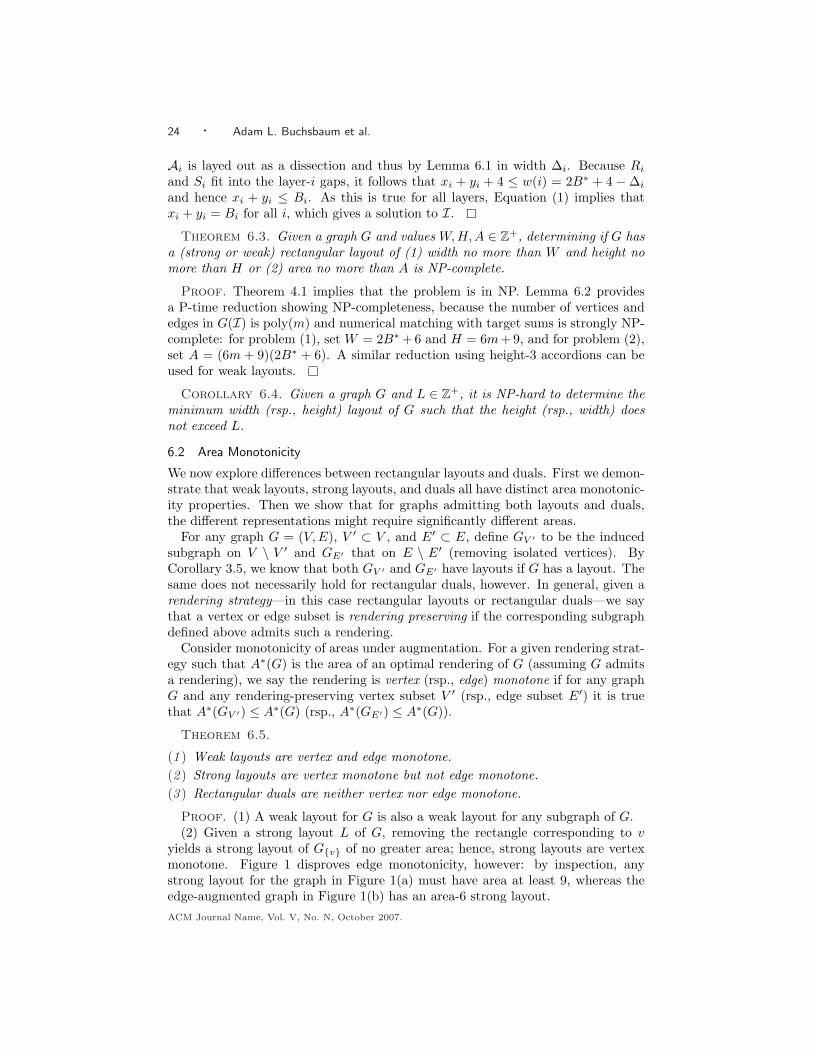
yields a strong layout of Gv of no greater area; hence, strong layouts are vertexmonotone. Figure 1 disproves edge monotonicity, however: by inspection, anystrong layout for the graph in Figure 1(a) must have area at least 9, whereas theedge-augmented graph in Figure 1(b) has an area-6 strong layout.ACM Journal Name, Vol. V, No. N, October 2007.


un−1

d

a b

cv1 vn

u2

un

x

u1

(a)

q

p

p

a

x

d

v1

b un u2

vn

c

u1q

(b)

Fig. 12. (a) A graph on 2n + 7 vertices. (b) A rectangular dual of area 6(n + 2).

un−1

d

a b

c

q

v1 vn

u2

un

x

u1

(a)

b

un

u2

u1

cvn

d

a

x

v1

v2

vn−

1

q

(b)

a

x

d v1

v2

vn−

1

vn

u2

un−

1

un

bq

c

u1

(c)

Fig. 13. (a) The graph on 2n + 6 vertices derived by deleting vertex p from Figure 12(a). (b) Arectangular dual of area (n + 3)(n + 2). (c) A strong rectangular layout of area 4(n + 2).

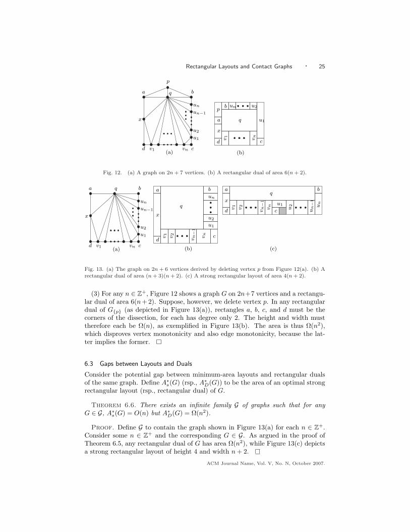
(3) For any n ∈ Z+, Figure 12 shows a graph G on 2n+7 vertices and a rectangu-lar dual of area 6(n + 2). Suppose, however, we delete vertex p. In any rectangulardual of Gp (as depicted in Figure 13(a)), rectangles a, b, c, and d must be thecorners of the dissection, for each has degree only 2. The height and width musttherefore each be Ω(n), as exemplified in Figure 13(b). The area is thus Ω(n2),which disproves vertex monotonicity and also edge monotonicity, because the lat-ter implies the former.

6.3 Gaps between Layouts and Duals

Consider the potential gap between minimum-area layouts and rectangular dualsof the same graph. Define A∗s(G) (rsp., A∗D(G)) to be the area of an optimal strongrectangular layout (rsp., rectangular dual) of G.

Theorem 6.6. There exists an infinite family G of graphs such that for anyG ∈ G, A∗s(G) = O(n) but A∗D(G) = Ω(n2).

Proof. Define G to contain the graph shown in Figure 13(a) for each n ∈ Z+.Consider some n ∈ Z+ and the corresponding G ∈ G. As argued in the proof ofTheorem 6.5, any rectangular dual of G has area Ω(n2), while Figure 13(c) depictsa strong rectangular layout of height 4 and width n + 2.



7. CONCLUSION

We have presented a new characterization of contact graphs of isothetic rectanglesin terms of those planar graphs that can be embedded with no filled three-cycles.We have shown the general area and constrained-width (and -height) optimizationproblems for rectangular layouts to be NP-hard and provided O(n)-time algorithmsto construct O(n2)-area rectangular layouts for graphs and O(n log n)-area rectan-gular layouts for trees.

Many open problems remain. What is the hardness of approximating the mi-nimum-area rectangular layout? Are there better approximation algorithms thanthe ones we presented here (O(n)-approximation for graphs; O(log n) for trees)? Isapproximating the minimum dimension (width or height) easier than approximatingthe area? This problem is motivated by applications on fixed-width, scrollabledisplays. Also, does the NP-hardness result extend to rectangular duals? Sincegraphs that admit such duals are internally triangulated (triangulated except forthe outer face), the freedom to place components to satisfy partition-type reductionsdoes not seem to exist.

Can our techniques be applied to study contact graphs on other closed shapes:for example, squares, arbitrary regular polygons, arbitrary convex polygons, andhigher-dimensional shapes? Also, allowing corner touching to imply adjacencychanges the class of graphs described by layouts. For example, K4 can be ex-pressed by four rectangles meeting at a corner, and K6, which is not planar, canbe expressed by triangles. For k ≥ 4, however, no layout on k-gons can expressa non-planar graph. Allowing corner touching also opens the question of allowingnon-isothetic rectangles, which can represent embeddings with filled triangles. Fi-nally, is there a class of polygonal shapes other than disks whose contact graphsare the planar graphs?

APPENDIX—Proofs of Lemmas

Lemma 2.2. A graph G is a 4-connected planar triangulation if and only if G∗ isplanar, cubic, and cyclically 4-edge connected.

Proof. G is a planar triangulation if and only if G∗ is planar and cubic. Ittherefore suffices to prove that (1) if G is a planar triangulation that is not 4-connected, then G∗ is not cyclically 4-edge connected, and (2) if G∗ is cubic andplanar but not cyclically 4-edge connected, then G is not 4-connected.

Assume that G is a planar triangulation that is not 4-connected. By Lemma 2.1G has some separating triangle (a, b, c). In G∗, therefore, there are edges a, b,b, c, and c, a, each connecting the two faces in G incident upon edges a, b,b, c, and c, a, resp. These three edges separate G∗ into two components, G∗1and G∗2. That (a, b, c) is a separating triangle and G is triangulated implies thatG∗1 and G∗2 contain cycles. Hence G∗ is not cyclically 4-edge connected.

Assume that G∗ is cubic and planar but not cyclically 4-edge connected. Thenthere exist three edges e1, e2, and e3 that separate G∗ into two or three components,each of which contains a cycle. Assume for now a separation into two components,G∗1 and G∗2. Without loss of generality, each of e1, e2, and e3 has an endpoint ineach component. Therefore there are vertices v1, v2, and v3 in G that correspondto the three faces induced in G∗ between pairs of e1, e2, and e3. Furthermore,ACM Journal Name, Vol. V, No. N, October 2007.


(v1, v2, v3) forms a separating triangle, because the cyclic nature of G∗1 and G∗2implies that the corresponding components G1 and G2 in G are non-empty. ByLemma 2.1, therefore, G, which is a planar triangulation, is not 4-connected. Asimilar argument holds when G∗ is separated into three components, in which casesome pair among e1, e2, and e3 separates G∗ into two components.

Lemma 3.1. A graph G is planar, cubic, and cyclically 4-edge connected if andonly if G is a saturated plane map with no 3-ring.

Proof. Assume G is a saturated plane map with no 3-ring. By definition, Gis cubic and planar, and so G∗ is a planar triangulation. Furthermore, because a3-ring in G induces a separating triangle in G∗ and vice-versa, it follows that G∗

has no separating triangle. By Lemma 2.1, therefore, G∗ is 4-connected, and byLemma 2.2, G is cubic, cyclically 4-edge connected.

Assume G is planar, cubic, and cyclically 4-edge connected. Then by Lemma2.2 G∗ is a 4-connected planar triangulation. By Lemma 2.1, G∗ has no separatingtriangle, and so G has no 3-ring. That G is a saturated plane map follows theassumption by definition.

ACKNOWLEDGMENTS

We thank Therese Biedl and Chandra Chekuri for fruitful discussions and AnneRogers for her tolerance. We thank the anonymous referees for many constructivecomments.

REFERENCES

Accornero, A., Ancona, M., and Varini, S. 2000. All separating triangles in a plane graph canbe optimally “broken” in polynomial time. International Journal of Foundations of ComputerScience 11, 3, 405–21.

Aho, A. V., Hopcroft, J. E., and Ullman, J. D. 1974. The Design and Analysis of ComputerAlgorithms. Addison-Wesley, Reading, MA.

Bhasker, J. and Sahni, S. 1988. A linear algorithm to find a rectangular dual of a planartriangulated graph. Algorithmica 3, 247–78.

Biedl, T., Bretscher, A., and Meijer, H. 1999. Rectangle of influence drawings of graphswithout filled 3-cycles. In Proc. 7th Int’l. Symp. on Graph Drawing ’99. Lecture Notes inComputer Science, vol. 1731. Springer-Verlag, 359–68.

Biedl, T., Kant, G., and Kaufmann, M. 1997. On triangulating planar graphs under thefour-connectivity constraint. Algorithmica 19, 427–46.

Brandstadt, A., Le, V. B., and Spinrad, J. P. 1999. Graph Classes: A Survey. SIAM Mono-graphs on Discrete Mathematics and Applications. SIAM, Philadelphia, PA.

de Berg, M., Carlsson, S., and Overmars, M. H. 1992. A general approach to dominance inthe plane. Journal of Algorithms 13, 2, 274–96.

de Fraysseix, H., de Mendez, P. O., and Rosenstiehl, P. 1994. On triangle contact graphs.Combinatorics, Probability and Computing 3, 233–246.

Di Battista, G., Eades, P., Tamassia, R., and Tollis, I. 1999. Graph Drawing: Algorithmsfor the Visualization of Graphs. Prentice-Hall, Upper Saddle River, NJ.

Di Battista, G., Lenhart, W., and Liotta, G. 1994. Proximity drawability: A survey. In Proc.Graph Drawing, DIMACS Int’l. Wks. (GD’94). Lecture Notes in Computer Science, vol. 894.Springer-Verlag, 328–39.

Gabow, H. N. 1990. Data structures for weighted matching and nearest common ancestors withlinking. In Proc. 1st ACM-SIAM Symp. on Discrete Algorithms. 434–43.



Gabriel, K. R. and Sokal, R. R. 1969. A new statistical approach to geographical analysis.Systematic Zoology 18, 54–64.

Garey, M. R. and Johnson, D. S. 1979. Computers and Intractability: A Guide to the Theoryof NP-Completeness. W.H. Freeman and Company, New York.

Harel, D. and Tarjan, R. E. 1984. Fast algorithms for finding nearest common ancestors. SIAMJournal on Computing 13, 2, 338–55.

He, X. 1993. On finding the rectangular duals of planar triangular graphs. SIAM Journal onComputing 22, 6, 1218–26.

He, X. 2001. A simple linear time algorithm for proper box rectangular drawings of plane graphs.Journal of Algorithms 40, 1, 82–101.

Hlineny, P. 1998. Classes and recognition of curve contact graphs. Journal of CombinatorialTheory (B) 74, 1, 87–103.

Hlineny, P. and Kratochvıl, J. 2001. Representing graphs by disks and balls (a survey ofrecognition-complexity results). Discrete Mathematics 229, 1-3, 101–24.

Jaromczyk, J. W. and Toussaint, G. T. 1992. Relative neighborhood graphs and their relatives.Proceedings of the IEEE 80, 1502–17.

Kant, G. and He, X. 1997. Regular edge labeling of 4-connected plane graphs and its applicationsin graph drawing problems. Theoretical Computer Science 172, 175–93.

Koebe, P. 1936. Kontaktprobleme der konformen Abbildung. Berichte uber die Verhand-lungender Sachsischen, Akad. Wiss., Math.-Phys. Klass 88, 141–64.

Kozminski, K. and Kinnen, W. 1985. Rectangular duals of planar graphs. Networks 15, 145–57.

Kozminski, K. and Kinnen, W. 1988. Rectangular dualization and rectangular dissections. IEEETransactions on Circuits and Systems 35, 11, 1401–16.

Lai, Y.-T. and Leinwand, S. M. 1988. Algorithms for floorplan design via rectangular dualiza-tion. IEEE Transactions on Computer-Aided Design 7, 1278–89.

Lai, Y.-T. and Leinwand, S. M. 1990. A theory of rectangular dual graphs. Algorithmica 5,467–83.

LaPaugh, A. S. 1980. Algorithms for integrated circuit layout: An analytic approach. Ph.D.thesis, M.I.T.

Liotta, G., Lubiw, A., Meijer, H., and Whitesides, S. H. 1998. The rectangle of influencedrawability problem. Computational Geometry: Theory and Applications 10, 1–22.

McKee, T. A. and McMorris, F. R. 1999. Topics in Intersection Graph Theory. SIAM Mono-graphs on Discrete Mathematics and Applications. SIAM, Philadelphia, PA.

Muller, D. E. and Preparata, F. P. 1978. Finding the intersection of two convex polyhedra.Theoretical Computer Science 7, 2, 217–36.

Munkres, J. R. 1999. Topology: A First Course. Prentice-Hall of India, New Delhi.

Overmars, M. H. and Wood, D. 1988. On rectangular visibility. Journal of Algorithms 9, 3,372–90.

Pan, P., Shi, W., and Liu, C. L. 1996. Area minimization for hierarchical floorplans. Algorith-mica 15, 550–71.

Rahman, M. S., Nakano, S.-I., and Nishizeki, T. 1998. Rectangular grid drawings of planegraphs. Computational Geometry: Theory and Applications 10, 3, 203–20.

Rahman, M. S., Nakano, S.-I., and Nishizeki, T. 2000. Box-rectangular drawings of planegraphs. Journal of Algorithms 37, 2, 363–98.

Rahman, M. S., Nishizeki, T., and Ghosh, S. 2004. Rectangular drawings of planar graphs.Journal of Algorithms 50, 1, 62–78.

Ramakrishnan, R. and Gehrke, J. 2000. Database Management Systems. McGraw-Hill, Boston,MA.

Read, R. C. 1987. A new method for drawing a graph given the cyclic order of the edges at eachvertex. Congressus Numerantium 56, 31–44.

Rosenstiehl, P. and Tarjan, R. E. 1986. Rectilinear planar layouts and bipolar orientations ofplanar graphs. Discrete Computational Geometry 1, 343–53.



Sachs, H. 1994. Coin graphs, polyhedra, and conformal mapping. Discrete Mathematics 134,133–8.

Schieber, B. and Vishkin, U. 1988. On finding lowest common ancestors: Simplification andparallelization. SIAM Journal on Computing 17, 6, 1253–62.

Shi, W. 1996. A fast algorithm for area minimization of slicing floorplans. IEEE Transactionson Computer-Aided Design of Integrated Circuits and Systems 15, 12, 1525–32.

Steadman, P. 1976. Graph-theoretic representation of architectural arrangement. In The Archi-tecture of Form, L. March, Ed. Cambridge University Press, London, New York, Melbourne,94–115.

Stockmeyer, L. 1983. Optimal orientations of cells in slicing floorplan designs. Information andControl 57, 91–101.

Sur-Kolay, S. and Bhattacharya, B. B. 1988. Inherent nonslicability of rectangular duals inVLSI floorplanning. In Proc. 8th Conf. on Foundations of Software Technology and TheoreticalComputer Science. Lecture Notes in Computer Science, vol. 338. Springer-Verlag, 88–107.

Sur-Kolay, S. and Bhattacharya, B. B. 1991. On the family of inherently nonslicible floorplansin VLSI layout design. In Proc. IEEE Int’l. Conf. on Circuits and Systems. Vol. 5. 2850–3.

Tani, K., Tsukiyama, S., Shinoda, S., and Shirakawa, I. 1991. On area-efficient drawings ofrectangular duals for VLSI floor-plan. Mathematical Programming 52, 29–43.

Tarjan, R. E. 1979. Applications of path compression on balanced trees. Journal of theACM 26, 4, 690–715.

Thomassen, C. 1984. Plane representations of graphs. In Progress in Graph Theory, J. A. Bondyand U. S. R. Murty, Eds. Academic Press, Canada, 43–69.

Thomassen, C. 1986. Interval representations of planar graphs. Journal of Combinatorial Theory(B) 40, 9–20.

Ungar, P. 1953. On diagrams representing maps. Journal of the London Mathematical Society 28,336–42.

West, D. B. 1996. Introduction to Graph Theory. Prentice-Hall, Upper Saddle River, NJ.

Whitney, H. 1933. 2-isomorphic graphs. American Journal of Mathematics 55, 245–54.

Wimer, S., Koren, I., and Cederbaum, I. 1988. Floorplans, planar graphs, and layouts. IEEETransactions on Circuits and Systems 35, 3, 267–78.

Yeap, G. K. and Sarrafzadeh, M. 1993. A unified approach to floorplan sizing and enumeration.IEEE Transactions on Computer-Aided Design of Integrated Circuits and Systems 12, 12,1858–67.

Yeap, G. K. and Sarrafzadeh, M. 1995. Sliceable floorplanning by graph dualization. SIAMJournal on Discrete Mathematics 8, 2, 258–80.

Received Month Year; revised Month Year; accepted Month Year


Documents

Rectangular Layouts and Contact Graphsadambuchsbaum.com/papers/rectlay.pdf · Rectangular Layouts and Contact Graphs ... architectural design, ... Previous works considered concepts