RecoNet: An Interpretable Neural Architecture for ...Recommender systems are a branch of machine learning with the goal of predicting preferred future actions for users, based on their

RecoNet: An Interpretable Neural Architecturefor Recommender Systems

Francesco Fusco1∗ , Michalis Vlachos1,2∗ , Vasileios Vasileiadis3 , KathrinWardatzky1 and Johannes Schneider4

1IBM Research AI2University of Lausanne

3ipQuants AG4University of Liechtenstein

{ffu,hri}@zurich.ibm.com, [email protected], [email protected], [email protected]

AbstractNeural systems offer high predictive accuracy butare plagued by long training times and low inter-pretability. We present a simple neural architecturefor recommender systems that lifts several of theseshortcomings. Firstly, the approach has a high pre-dictive power that is comparable to state-of-the-artrecommender approaches. Secondly, owing to itssimplicity, the trained model can be interpreted eas-ily because it provides the individual contributionof each input feature to the decision. Our methodis three orders of magnitude faster than general-purpose explanatory approaches, such as LIME. Fi-nally, thanks to its design, our architecture addressescold-start issues, and therefore the model does notrequire retraining in the presence of new users.

1 IntroductionRecommender systems are a branch of machine learning withthe goal of predicting preferred future actions for users, basedon their historical preferences and individual traits (e.g. age,gender, location). E-commerce is one area that has been trans-formed by recommender systems, which provide a solutionto the information deluge problem: users are presented onlywith a list of likely future actions (items to purchase, videosto view, etc.), ranked by estimated interest to the user. Today,recommender systems and machine learning are penetratingand transforming many fields, including business [Heckel etal., 2017], finance [Yu et al., 2008], medicine/biology [Nevesand Leser, 2015], and law [Surden, 2014]. In many of thesedisciplines, it is essential not only to have accurate predictionsbut also to provide a rationale behind the decision that can bemade transparent to the end-user [Lipton, 2016]. Therefore,it is becoming increasingly important to deliver systems thatprovide both accuracy and interpretability.

Recently, deep-learning architectures have been adaptedto the context of recommender systems. These architectures

∗Corresponding authors; work conducted while at IBM Research.From June 2019, M. Vlachos is affiliated with the University ofLausanne, Department of Business and Economics.

exhibit improvements in predictive accuracy compared withexisting state-of-the-art methodologies based on matrix factor-ization, particularly in the case of cold-start problems. How-ever, deep learning still falls short in terms of interpretability,and it is quite challenging to rationalize why the recommenda-tion process elected a particular action.

We will address this limitation and propose a neural ar-chitecture tailored specifically to recommender systems thatcan retrace the contribution of the original features leadingto a given decision. We achieve this by building on notionsfrom relevance propagation methodologies, which have beensuccessful in the domain of image data [Bach et al., 2015].Contributions of this work include:

1. We propose a simple neural-network architecture to en-code user-item interactions and user or item features. Thearchitecture departs from the traditional inner product cal-culation, given the learned user and item embeddings. Toaccommodate for the inherent data sparsity in recommenda-tion settings and to allow the network to generalize betterunder cold-start conditions [Vartak et al., 2017], we introducea perturbation mechanism in the training process.

2. Owing to the simple topology, it is also possible tounderstand fully the individual contributions of the originalinput attributes for the network’s decisions. We achieve thisby adapting on ideas of relevance propagation, which propa-gate backwards the relevance of the network function outputthrough the network. To the best of our knowledge, this is thefirst effort of its kind in the field of recommender systems.

3. Our experiments show that: (a) The accuracy of thetechnique is comparable to existing state-of-the-art approaches.(b) Cold-start situations are well addressed. (c) We evaluatethe pertinence of the features returned by our methodology bymeans of significance testing and show their high relevanceto the decision made. (d) RecoNet offers equivalent or betterinterpretability than surrogate methodology approaches suchas LIME [Ribeiro et al., 2016], but at a fraction of the cost.

2 Our Recommender SettingLet us assume a set of n users U = {u1, . . . , un} and a setof m items V = {v1, . . . , vm}. For each user u, we havecollected her preference Ruv for an item v. In our setting, weassume that the preference is inferred from an implicit interac-

Proceedings of the Twenty-Eighth International Joint Conference on Artificial Intelligence (IJCAI-19)

2343

tion or feedback (e.g. product purchase, view of a movie, likeof an item page), which makes the n ×m matrix R binary.The problem of generating recommendations based on implicitfeedback is known as one-class collaborative filtering (OCCF).We denote the user history by V (u) = {v ∈ V |Ruv 6= 0}, i.e.the subset of items with which user u interacted.

Let us also assume that content information is available tousers and items. User features such as gender, age, location,etc. are usually known, whereas for items, one might havetextual information such as reviews, or categorical informationsuch as genres, numerical characteristics or images. We as-sume that, although we might have users or items with zero in-teractions (cold-start problem), we have a complete user/itemprofile. We denote by ΦU and ΦV the sets of user and itemfeatures, respectively. The features of a specific user u ∈ Uare denoted by the set ΦU (u) = {φu,1, . . . , φu,k}, whereφu,i ∈ ΦU , i = 1, . . . , k. We define the set of item featuresΦV (v) for a specific item v ∈ V in a similar way. We assumethat a user u can be adequately represented by all the infor-mation we have collected about her. Thus, the user’s featuresΦU (u), interactions V (u), and the features of the items withwhich the user has interacted ΦV (V (u)) =

⋃v∈V (u)

ΦV (v)

will be the input for our model. There is no overlap betweenitems and user or their respective features, ie., the feature setsΦV and ΦU as well as the item set V are pairwise disjoint.

3 Related WorkMuch of the work on recommender systems in the past decadehas focused on matrix factorization (MF) approaches [Ko-ren et al., 2009]. MF techniques operate by describing usersand items in a latent dimensionality and modelling the in-teractions between users and items through an inner-productcomputation. MF can predict ratings or preferences well,but the latent feature space makes it difficult to explain rec-ommendations. Recently, deep neural network (DNN) ar-chitectures have also been applied in the area of recom-mender systems. Several variants of DNNs have been pre-sented previously [He and Chua, 2017; He et al., 2017;Cheng et al., 2016; Shan et al., 2016; X. Wang and Chua, 2017;Zhang et al., 2016]. In these works, we can distinguish twomain paths of modeling the structure of the DNN. One pathfollows ideas built on embeddings, combining the resultingfeatures with deeper pooling or stacking of the resulting neu-ral layers, and the classification is typically accomplishedusing some variant of a logistic regression or nearest-neighborsearch. The second path follows a core idea very similar tomatrix factorization and tries to model the interaction betweenusers and items using an inner-product calculation. The dif-ference to MF approaches is that the neural network learnsthe new latent space of users and items. However, none ofthe works in recommender systems based on neural networksexplicitly address the topic of interpretability. In contrast, ourwork describes a neural recommender system designed fromthe ground up to provide interpretable results.

Our network architecture shares commonalities with word-embedding approaches such as word2vec [Mikolov et al.,2013a] and other shallow networks for classification tasks

(FastText [Bojanowski et al., 2017] and StarSpace [Wu etal., 2017]). A significant difference is that our work not onlypredicts a class given a set of features, but also highlights and—more importantly—ranks the set of features (i.e. items andattributes) that contributed most to the classification output.

Relevance propagation (or attribution) methods have beenproposed and, so far, applied predominantly in the context ofimages to understand the contribution of each input feature ina deep neural network to the classification output. Attributionmethods include approaches such as salience maps [Simonyanet al., 2013; Baehrens et al., 2010], layerwise relevance propa-gation (LRP) [Bach et al., 2015] and DeepLIFT [Shrikumar etal., 2017]. We review how such approaches operate. Let usconsider a network with input x = [x1, . . . , xn], which pro-duces an output of f(x) = [f1(x), . . . , fC(x)], where C is thenumber of output neurons. Given a target neuron c ∈ C , thepurpose is to determine the relevance R = [R1, . . . , Rn] ofeach input feature xk to the output fc. Salience maps decom-pose the gradient-squared norm of the output function as a sumof relevances of the input features, i.e.

∑iRi = ||∇f(x)||,

helping to measure how much the changes in each pixel con-tribute to the prediction. LRP decomposes the classificationdecision into pixel-wise relevances, i.e.

∑iRi = f(x), thus

indicating the contributions of each pixel to the overall classi-fication score. LRP operates using a layer-wise conservationprinciple, forcing the total sum of relevances to be preservedbetween neurons of two consecutive layers. Finally, DeepLIFToperates in a backward fashion similar to LRP, decomposingthe output prediction of a neural network for a particular inputby back-propagating the contributions of all neurons in the net-work to each input feature. An effort to provide a unified viewof the proposed relevance propagation methods has appearedin [Ancona et al., 2017].

Unlike attribution methods, surrogate model approaches canbe applied to any pre-existing model, i.e., the original modelis treated as a black-box. We compare our approach withLIME [Ribeiro et al., 2016], a well-established and widelyused surrogate technique, in Section 5.5.

4 Our ApproachThe main objective of our research is to engineer a recom-mender system that not only delivers high-quality recommen-dations, but is also capable of identifying the individual itemsor additional attributes that contributed to the recommenda-tion. Therefore, our goal is to move beyond existing MF-basedapproaches, which are not able to rank individual items andfeatures by importance, and beyond current deep-learning rec-ommenders, which are difficult to explain and require black-box explanatory tools to generate the explanations.

One of the main challenges to explainability that affectsexisting deep-learning recommenders comes from the fact thatusers, items and attributes are not treated homogeneously. Forexample, embedding-based approaches project each user andattribute into a different space. In our work, users are identifiedby a set of items and attributes (i.e. each user can be identifiedby a bitmap), and the user representation is computed byaveraging embedding vectors corresponding to each one ofthe items and attributes associated to that user.


2344

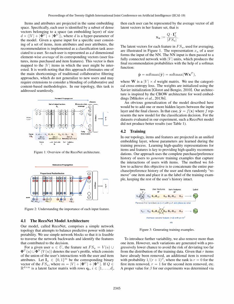
Items and attributes are projected in the same embeddingspace. Specifically, each user is identified by a subset of densevectors belonging to a space (an embedding layer) of sized × (|V | + |ΦU | + |ΦV |), where d is a hyper-parameter ofthe model. Given a sparse input for a specific user consist-ing of a set of items, item attributes and user attributes, therecommendation is implemented as a classification task asso-ciated to a user. So each user is represented as a d-dimensionalelement-wise average of its corresponding vectors (user fea-tures, items purchased and item features). This vector is thenmapped to the |V | items in which the user might be inter-ested. It is worth noting that this approach eliminates one ofthe main shortcomings of traditional collaborative filteringapproaches, which do not generalize to new users and mayrequire extensions to consider a blending of collaborative andcontent-based methodologies. In our topology, this task isaddressed seamlessly.

Figure 1: Overview of the RecoNet architecture.

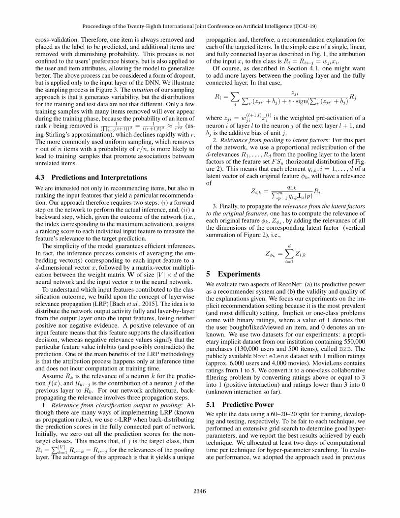
Figure 2: Understanding the importance of each input feature.

4.1 The RecoNet Model ArchitectureOur model, called RecoNet, comprises a simple networktopology that attempts to balance predictive power with inter-pretability. We use simple network blocks so that it is feasibleto traverse the network backwards and identify the featuresthat contributed to the decision.

For a given user u ∈ U , the feature set FSu = V (u) ∪ΦU (u)∪ΦV (V (u)) denotes the user’s profile, which consistsof the union of the user’s interactions with the user and itemattributes. Let Iu ∈ {0, 1}m be the corresponding binaryvector of the FSu, where m = |V | + |ΦU | + |ΦV |. If Q ∈Rd×m is a latent factor matrix with rows qi, i ∈ [1, . . . , d],

then each user can be represented by the average vector of alllatent vectors in her feature set, that is

xu :=Q · ITu|FSu|

.

The latent vectors for each feature in FSu, used for averaging,are illustrated in Figure 1. The representation xu of a userforms the input of the NN. The NN input is then passed to afully connected network with |V | units, which produces thefinal recommendation probabilities with the help of a softmaxfunction:

p = softmax(y) = softmax(WxT ),

where W is a |V | × d weight matrix. We use the categori-cal cross-entropy loss. The weights are initialized using theXavier initialization [Glorot and Bengio, 2010]. Our architec-ture is inspired by the CBOW architecture for word embed-dings [Mikolov et al., 2013b].

An obvious generalization of the model described herewould be to add one or more hidden layers between the inputlayer and the final classes. In that case, y = f(x) where f rep-resents the new model for the classification decision. For thedatasets evaluated in our experiment, such a RecoNet modeldid not produce better results (see Table 1).

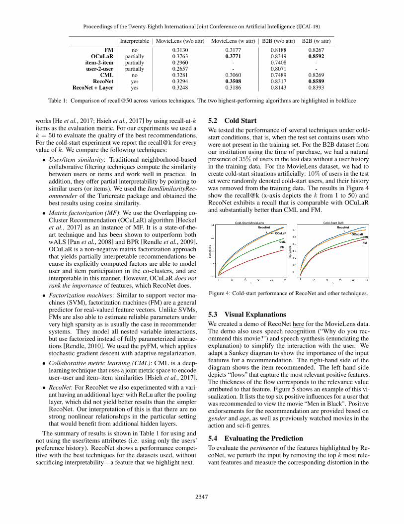
4.2 TrainingIn our topology, items and features are projected in an unifiedembedding layer, whose parameters are learned during thetraining process. Learning high-quality representations foritems and features is key to providing high-quality recommen-dations. Our approach uses the complete purchase/preferencehistory of users to generate training examples that capturethe interactions of users with items. The method we fol-low to achieve this objective is to concatenate the entire pur-chase/preference history of the user and then randomly “re-move” one item and place it as the label of the training exam-ple, keeping the rest of the user’s history intact.

Figure 3: Generating training examples.

To introduce further variability, we also remove more thanone item. However, such variations are generated with a pro-gressively lower chance to avoid the risk of deviating too farfrom the distribution of the training data. Given that r itemshave already been removed, an additional item is removedwith probability 1/(r + 1)β , where the rank is r = 0 for thefirst item removed, r = 1 for the second item removed, etc.A proper value for β for our experiments was determined via


2345

cross-validation. Therefore, one item is always removed andplaced as the label to be predicted, and additional items areremoved with diminishing probability. This process is notconfined to the users’ preference history, but is also applied tothe user and item attributes, allowing the model to generalizebetter. The above process can be considered a form of dropout,but is applied only to the input layer of the DNN. We illustratethe sampling process in Figure 3. The intuition of our samplingapproach is that it generates variability, but the distributionsfor the training and test data are not that different. Only a fewtraining samples with many items removed will ever appearduring the training phase, because the probability of an item ofrank r being removed is 1

(∏ri=0(i+1))β

= 1((r+1)!)β

≈ 1rrβ

(us-ing Stirling’s approximation), which declines rapidly with r.The more commonly used uniform sampling, which removesr out of n items with a probability of r/n, is more likely tolead to training samples that promote associations betweenunrelated items.

4.3 Predictions and InterpretationsWe are interested not only in recommending items, but also inranking the input features that yield a particular recommenda-tion. Our approach therefore requires two steps: (i) a forwardstep on the network to perform the actual inference, and, (ii) abackward step, which, given the outcome of the network (i.e.,the index corresponding to the maximum activation), assignsa ranking score to each individual input feature to measure thefeature’s relevance to the target prediction.

The simplicity of the model guarantees efficient inferences.In fact, the inference process consists of averaging the em-bedding vector(s) corresponding to each input feature to ad-dimensional vector x, followed by a matrix-vector multipli-cation between the weight matrix W of size |V | × d of theneural network and the input vector x to the neural network.

To understand which input features contributed to the clas-sification outcome, we build upon the concept of layerwiserelevance propagation (LRP) [Bach et al., 2015]. The idea is todistribute the network output activity fully and layer-by-layerfrom the output layer onto the input features, losing neitherpositive nor negative evidence. A positive relevance of aninput feature means that this feature supports the classificationdecision, whereas negative relevance values signify that theparticular feature value inhibits (and possibly contradicts) theprediction. One of the main benefits of the LRP methodologyis that the attribution process happens only at inference timeand does not incur computation at training time.

Assume Rk is the relevance of a neuron k for the predic-tion f(x), and Rk←j is the contribution of a neuron j of theprevious layer to Rk. For our network architecture, back-propagating the relevance involves three propagation steps.

1. Relevance from classification output to pooling: Al-though there are many ways of implementing LRP (knownas propagation rules), we use ε-LRP when back-distributingthe prediction scores in the fully connected part of network.Initially, we zero out all the prediction scores for the non-target classes. This means that, if j is the target class, thenRi =

∑|V |k=1Ri←k = Ri←j for the relevances of the pooling

layer. The advantage of this approach is that it yields a unique

propagation and, therefore, a recommendation explanation foreach of the targeted items. In the simple case of a single, linear,and fully connected layer as described in Fig. 1, the attributionof the input xi to this class is Ri = Ri←j = wjixi.

Of course, as described in Section 4.1, one might wantto add more layers between the pooling layer and the fullyconnected layer. In that case,

Ri =∑j

zji∑i′(zji′ + bj) + ε · sign(

∑i′(zji′ + bj)

Rj

where zji = w(l+1,l)ji x

(l)i is the weighted pre-activation of a

neuron i of layer l to the neuron j of the next layer l + 1, andbj is the additive bias of unit j.

2. Relevance from pooling to latent factors: For this partof the network, we use a proportional redistribution of thed-relevances R1, . . . , Rd from the pooling layer to the latentfactors of the feature set FSu (horizontal distribution of Fig-ure 2). This means that each element qi,k, i = 1, . . . , d of alatent vector of each original feature φk, will have a relevanceof

Zi,k =qi,k∑m

p=1 qi,pIu(p)Ri

3. Finally, to propagate the relevance from the latent factorsto the original features, one has to compute the relevance ofeach original feature φk, Zφk , by adding the relevances of allthe dimensions of the corresponding latent factor (verticalsummation of Figure 2), i.e.,

Zφk =d∑i=1

Zi,k

5 ExperimentsWe evaluate two aspects of RecoNet: (a) its predictive poweras a recommender system and (b) the validity and quality ofthe explanations given. We focus our experiments on the im-plicit recommendation setting because it is the most prevalent(and most difficult) setting. Implicit or one-class problemscome with binary ratings, where a value of 1 denotes thatthe user bought/liked/viewed an item, and 0 denotes an un-known. We use two datasets for our experiments: a propri-etary implicit dataset from our institution containing 550,000purchases (130,000 users and 500 items), called B2B. Thepublicly available MovieLens dataset with 1 million ratings(approx. 6,000 users and 4,000 movies). MovieLens containsratings from 1 to 5. We convert it to a one-class collaborativefiltering problem by converting ratings above or equal to 3into 1 (positive interaction) and ratings lower than 3 into 0(unknown interaction so far).

5.1 Predictive PowerWe split the data using a 60–20–20 split for training, develop-ing and testing, respectively. To be fair to each technique, weperformed an extensive grid search to determine good hyper-parameters, and we report the best results achieved by eachtechnique. We allocated at least two days of computationaltime per technique for hyper-parameter searching. To evalu-ate performance, we adopted the approach used in previous


2346

Interpretable MovieLens (w/o attr) MovieLens (w attr) B2B (w/o attr) B2B (w attr)

FM no 0.3130 0.3177 0.8188 0.8267OCuLaR partially 0.3763 0.3771 0.8349 0.8592

item-2-item partially 0.2960 - 0.7408 -user-2-user partially 0.2657 - 0.8071 -

CML no 0.3281 0.3060 0.7489 0.8269RecoNet yes 0.3294 0.3508 0.8317 0.8589

RecoNet + Layer yes 0.3248 0.3186 0.8143 0.8393

Table 1: Comparison of recall@50 across various techniques. The two highest-performing algorithms are highlighted in boldface

works [He et al., 2017; Hsieh et al., 2017] by using recall-at-kitems as the evaluation metric. For our experiments we used ak = 50 to evaluate the quality of the best recommendations.For the cold-start experiment we report the recall@k for everyvalue of k. We compare the following techniques:• User/item similarity: Traditional neighborhood-based

collaborative filtering techniques compute the similaritybetween users or items and work well in practice. Inaddition, they offer partial interpretability by pointing tosimilar users (or items). We used the ItemSimilarityRec-ommender of the Turicreate package and obtained thebest results using cosine similarity.• Matrix factorization (MF): We use the Overlapping co-

Cluster Recommendation (OCuLaR) algorithm [Heckelet al., 2017] as an instance of MF. It is a state-of-the-art technique and has been shown to outperform bothwALS [Pan et al., 2008] and BPR [Rendle et al., 2009].OCuLaR is a non-negative matrix factorization approachthat yields partially interpretable recommendations be-cause its explicitly computed factors are able to modeluser and item participation in the co-clusters, and areinterpretable in this manner. However, OCuLaR does notrank the importance of features, which RecoNet does.• Factorization machines: Similar to support vector ma-

chines (SVM), factorization machines (FM) are a generalpredictor for real-valued feature vectors. Unlike SVMs,FMs are also able to estimate reliable parameters undervery high sparsity as is usually the case in recommendersystems. They model all nested variable interactions,but use factorized instead of fully parameterized interac-tions [Rendle, 2010]. We used the pyFM, which appliesstochastic gradient descent with adaptive regularization.• Collaborative metric learning (CML): CML is a deep-

learning technique that uses a joint metric space to encodeuser–user and item–item similarities [Hsieh et al., 2017].• RecoNet: For RecoNet we also experimented with a vari-

ant having an additional layer with ReLu after the poolinglayer, which did not yield better results than the simplerRecoNet. Our interpretation of this is that there are nostrong nonlinear relationships in the particular settingthat would benefit from additional hidden layers.

The summary of results is shown in Table 1 for using andnot using the user/items attributes (i.e. using only the users’preference history). RecoNet shows a performance compet-itive with the best techniques for the datasets used, withoutsacrificing interpretability—a feature that we highlight next.

5.2 Cold StartWe tested the performance of several techniques under cold-start conditions, that is, when the test set contains users whowere not present in the training set. For the B2B dataset fromour institution using the time of purchase, we had a naturalpresence of 35% of users in the test data without a user historyin the training data. For the MovieLens dataset, we had tocreate cold-start situations artificially: 10% of users in the testset were randomly denoted cold-start users, and their historywas removed from the training data. The results in Figure 4show the recall@k (x-axis depicts the k from 1 to 50) andRecoNet exhibits a recall that is comparable with OCuLaRand substantially better than CML and FM.

Cold-Start MovieLens Cold-Start B2B

Rec

all@

k

Rec

all@

k

RecoNet

FM

RecoNet

FMCML

OCuLaR OCuLaRCML

Figure 4: Cold-start performance of RecoNet and other techniques.

5.3 Visual ExplanationsWe created a demo of RecoNet here for the MovieLens data.The demo also uses speech recognition (“Why do you rec-ommend this movie?") and speech synthesis (enunciating theexplanation) to simplify the interaction with the user. Weadapt a Sankey diagram to show the importance of the inputfeatures for a recommendation. The right-hand side of thediagram shows the item recommended. The left-hand sidedepicts “flows” that capture the most relevant positive features.The thickness of the flow corresponds to the relevance valueattributed to that feature. Figure 5 shows an example of this vi-sualization. It lists the top six positive influences for a user thatwas recommended to view the movie “Men in Black". Positiveendorsements for the recommendation are provided based ongender and age, as well as previously watched movies in theaction and sci-fi genres.

5.4 Evaluating the PredictionTo evaluate the pertinence of the features highlighted by Re-coNet, we perturb the input by removing the top k most rele-vant features and measure the corresponding distortion in the


2347

Figure 5: Example of a movie recommendation. The top relevantoriginal features that contributed to this decision are highlighted.

classification output. We measure for each k the effect of theperturbation on the target activation, i.e. ∆yc = fc(x|xk =0)− fc(x), where the former part indicates that the top k-thfeatures have been removed from input x. We compare the dis-tribution of ∆yc when the top k removed features are selectedat random or using the ranking provided by RecoNet. Figure 6shows the estimated mean difference of the activation of therecommended item after perturbing the top 50 most relevantattributes for both datasets. The gray band represents the 95%confidence interval of the estimated mean. It is obvious that,for both datasets, removing the most relevant features signifi-cantly decreases the activation value of the targeted output.

MovieLens B2B

perturbation steps perturbation steps

Random

RecoNetRecoNet

Random

Figure 6: The large drop suggests that removing the features deemedimportant by RecoNet greatly affects the classification output.

Previous work followed equivalent methodologies [Anconaet al., 2017; Bach et al., 2015] to quantify the validity ofthe selected features. We provide a stronger result through aformal test of statistical significance. Figure 7 compares thedistribution of ∆yc when perturbing a random input feature(labeled “random 1”) and compares it with the distribution forthe case where we perturb the feature that was highlighted asthe most important (labeled “top 1”). The shape of the distri-butions is different: the “top 1‘’ is negatively skewed, whereasthe “random 1” is more symmetric. We test the hypothesiswhether the samples come from the same distributions usingthe Mann–Whitney U test. The p-value is less than 10−4 forboth datasets; the hypothesis cannot be accepted.

5.5 RecoNet vs LIMELIME [Ribeiro et al., 2016] is a well-established surrogatetechnique for interpreting the output of classifiers. LIMEexplains a classification instance by building a surrogate ex-plainable model that locally approximates the particular classi-fication output. To have a strong baseline for our approach, we

−2 −1 0 1∆ y

500

1000

1500

2000

2500

3000MovieLens

top 1

random 1

−15 −10 −5 0 5∆ y

0

5000

10000

15000

20000

25000

30000B2B

top 1

random 1

Figure 7: Comparison of the distributions of ∆y for the top recom-mendation in two cases: (a) when the most relevant feature (“top 1”)is perturbed and (b) when a random feature (“random 1”) is modified.

implemented an alternate explanation engine built on LIME(and RecoNet as its black-box model). In Figure 8 we repeatthe experiment shown in Figure 6, focusing only on RecoNetand LIME. This figure highlights the very good agreement forboth techniques among the first four to five features rankedmost important. For the remaining features, RecoNet exhibitsa larger decrease than LIME in the classifier output whenthese features are removed, suggesting that the features rankedhighest by RecoNet were indeed more important than thosediscovered by LIME.

1. 'Pulp Fiction (1994)'2. 'Usual Suspects, The (1995)'3. 'Sixth Sense, The (1999)'4. 'Few Good Men, A (1992)'5. 'Full Monty, The (1997)'6. 'zipcode - 55416'7. 'Hoop Dreams (1994)'8. 'Antz (1998)'9. 'Cop Land (1997)'10. ‘Attribute – Occupation’11. 'Shawshank Redemption (1994)'12. 'Game (1997)'

RecoNet: top features LIME: top features

1. 'Pulp Fiction (1994)'2. 'Usual Suspects, The (1995)'3. 'Sixth Sense, The (1999)'4. 'Antz (1998)’5. 'Full Monty, The (1997)’6. 'Hoop Dreams (1994)’7. 'Few Good Men, A (1992)’8. 'zipcode - 55416'9. 'Cop Land (1997)'10. ‘Attribute – Occupation’11. 'Strictly Ballroom (1992)'12. 'gender – Male’

ExampleRecommendation

Reasoning for Recommendationperturbation steps

MovieLens

LIME

RecoNet

Figure 8: Left: The greater decrease for RecoNet shows that thefeatures selected are more descriptive than those indicated by LIME.Right: A good agreement of feature importance for LIME and Re-coNet for a recommendation instance for the movie “Fargo”.

RecoNet has been designed from the ground up to provideinterpretable recommendations without substantially increas-ing the inference latency. LIME, on the other hand, incursa large per-inference cost, and it can be impractical for usein industrial and multi-user applications. In fact, for each ex-planation, LIME probes several thousands of inferences onthe black-box model. For example, to generate the explana-tions for each recommendation instance in our setup, LIMErequired an average of 10–12 seconds. RecoNet required onaverage 10 milliseconds to perform the inference and generatethe explanation; thus, it is more than 1000 times faster.

6 Conclusion

RecoNet is a neural recommender system that (a) exhibitspredictive power that is competitive with state-of-the-art rec-ommendation approaches, (b) is explainable, (c) can addresscold-start situations. Our experiments suggest that the origi-nal features highlighted as relevant are indeed pertinent andstatistically significant.


2348

References[Ancona et al., 2017] Marco Ancona, Enea Ceolini, Cengiz

Öztireli, and Markus Gross. A unified view of gradient-based attribution methods for deep neural networks. NIPSworkshop on Interpreting, Explaining and Visualizing DeepLearning, 2017.

[Bach et al., 2015] Sebastian Bach, Alexander Binder, Gré-goire Montavon, Frederick Klauschen, Klaus-RobertMüller, and Wojciech Samek. On pixel-wise explanationsfor non-linear classifier decisions by layer-wise relevancepropagation. PloS one, 10(7):e0130140, 2015.

[Baehrens et al., 2010] David Baehrens, Timon Schroeter,Stefan Harmeling, Motoaki Kawanabe, Katja Hansen, andKlaus-Robert MÃžller. How to explain individual classifi-cation decisions. Journal of Machine Learning Research,11:1803–1831, 2010.

[Bojanowski et al., 2017] Piotr Bojanowski, Edouard Grave,Armand Joulin, and Tomas Mikolov. Enriching word vec-tors with subword information. Transactions of the Associ-ation for Computational Linguistics, 5:135–146, 2017.

[Cheng et al., 2016] Heng-Tze Cheng, Levent Koc, JeremiahHarmsen, Tal Shaked, Tushar Chandra, Hrishi Aradhye,Glen Anderson, Greg Corrado, Wei Chai, Mustafa Ispir,Rohan Anil, Zakaria Haque, Lichan Hong, Vihan Jain,Xiaobing Liu, and Hemal Shah. Wide & deep learning forrecommender systems. In Workshop on Deep Learning forRecommender Systems, pages 7–10, 2016.

[Glorot and Bengio, 2010] Xavier Glorot and Yoshua Bengio.Understanding the difficulty of training deep feedforwardneural networks. In International Conference on ArtificialIntelligence and Statistics, AISTATS, pages 249–256, 2010.

[He and Chua, 2017] Xiangnan He and Tat-Seng Chua. Neu-ral factorization machines for sparse predictive analytics.In Proc. SIGIR, pages 355–364, 2017.

[He et al., 2017] Xiangnan He, Lizi Liao, Hanwang Zhang,Liqiang Nie, Xia Hu, and Tat-Seng Chua. Neural collabo-rative filtering. In Proc. WWW, pages 173–182, 2017.

[Heckel et al., 2017] Reinhard Heckel, Michail Vlachos,Thomas P. Parnell, and Celestine Dünner. Scalable andinterpretable product recommendations via overlapping co-clustering. In Proc. IEEE ICDE, pages 1033–1044, 2017.

[Hsieh et al., 2017] Cheng-Kang Hsieh, Longqi Yang, YinCui, Tsung-Yi Lin, Serge J. Belongie, and Deborah Estrin.Collaborative metric learning. In Proc. WWW, pages 193–201, 2017.

[Koren et al., 2009] Yehuda Koren, Robert Bell, and ChrisVolinsky. Matrix factorization techniques for recommendersystems. Computer, 42(8):30–37, August 2009.

[Lipton, 2016] Zachary C Lipton. The mythos of model in-terpretability. arXiv preprint arXiv:1606.03490, 2016.

[Mikolov et al., 2013a] Tomas Mikolov, Kai Chen, Greg Cor-rado, and Jeffrey Dean. Efficient estimation of word repre-sentations in vector space. CoRR, abs/1301.3781, 2013.

[Mikolov et al., 2013b] Tomas Mikolov, Kai Chen, Greg Cor-rado, and Jeffrey Dean. Efficient estimation of word repre-sentations in vector space. arXiv preprint arXiv:1301.3781,2013.

[Neves and Leser, 2015] Mariana Neves and Ulf Leser. Ques-tion answering for biology. Methods, 74:36–46, 2015.

[Pan et al., 2008] Rong Pan, Yunhong Zhou, Bin Cao, N.N.Liu, R. Lukose, M. Scholz, and Qiang Yang. One-classcollaborative filtering. In Proc. ICDM, pages 502–511,2008.

[Rendle et al., 2009] Steffen Rendle, Christoph Freuden-thaler, Zeno Gantner, and Lars Schmidt-Thieme. BPR:bayesian personalized ranking from implicit feedback. InProc. UAI, pages 452–461, 2009.

[Rendle, 2010] Steffen Rendle. Factorization machines. InProc. ICDM, pages 995–1000, 2010.

[Ribeiro et al., 2016] Marco Túlio Ribeiro, Sameer Singh,and Carlos Guestrin. "why should I trust you?": Explainingthe predictions of any classifier. In Proc. ACM SIGKDD,pages 1135–1144, 2016.

[Shan et al., 2016] Ying Shan, T. Ryan Hoens, Jian Jiao, Hai-jing Wang, Dong Yu, and JC Mao. Deep crossing: Web-scale modeling without manually crafted combinatorialfeatures. In Proc. ACM SIGKDD, pages 255–262, 2016.

[Shrikumar et al., 2017] Avanti Shrikumar, Peyton Green-side, and Anshul Kundaje. Learning important featuresthrough propagating activation differences. arXiv preprintarXiv:1704.02685, 2017.

[Simonyan et al., 2013] Karen Simonyan, Andrea Vedaldi,and Andrew Zisserman. Deep inside convolutional net-works: Visualising image classification models and saliencymaps. CoRR, abs/1312.6034, 2013.

[Surden, 2014] Harry Surden. Machine learning and law.Washington Law Review, 89(1), 2014.

[Vartak et al., 2017] Manasi Vartak, Arvind Thiagarajan,Conrado Miranda, Jeshua Bratman, and Hugo Larochelle.A meta-learning perspective on cold-start recommendationsfor items. In NIPS, pages 6904–6914. 2017.

[Wu et al., 2017] Ledell Wu, Adam Fisch, Sumit Chopra,Keith Adams, Antoine Bordes, and Jason Weston.Starspace: Embed all the things! CoRR, abs/1709.03856,2017.

[X. Wang and Chua, 2017] L. Nie X. Wang, X. He and T.-S.Chua. Item silk road: Recommending items from infor-mation domains to social users. In Proc. of SIGIR, pages185–194, 2017.

[Yu et al., 2008] Lean Yu, Shouyang Wang, and Kin KeungLai. Credit risk assessment with a multistage neural net-work ensemble learning approach. Expert systems withapplications, 34(2):1434–1444, 2008.

[Zhang et al., 2016] Weinan Zhang, Tianming Du, and JunWang. Deep learning over multi-field categorical data. InAdvances in Information Retrieval, pages 45–57, 2016.


2349

Documents

RecoNet: An Interpretable Neural Architecture for ...Recommender systems are a branch of machine learning with the goal of predicting preferred future actions for users, based on their