Interpretable Linear Modeling - Piazza

InterpretableLinear Modeling

Jeffrey M. GirardCarnegie Mellon University

LM GLM MLM

11/19/2019 Interpretable Linear Modeling 2

Overview

Linear Modeling

Generalized Linear Modeling

Multilevel Modeling

Linear Modeling

• Linear models (LM) are statistical prediction models with high interpretability• They are best combined with a small number of interpretable features• They allow you to quantify the size and direction of each feature's effect• They allow you to isolate the unique effect of each feature

• LM incorporates regression, ANOVA, 𝑡𝑡-tests, and 𝐹𝐹-tests• LM allows for multiple 𝑋𝑋 (predictor or independent) variables• LM allows for multiple 𝑌𝑌 (explained or dependent) variables

• LM assumes the Y variables are normally distributed (to avoid → GLM)• LM assumes the data points are independent (to avoid → MLM)


What is linear modeling?

• Linear regression is often presented with the following notation:

𝑦𝑦𝑖𝑖 = 𝛼𝛼 + 𝛽𝛽1𝑥𝑥1𝑖𝑖 + ⋯+ 𝛽𝛽𝑝𝑝𝑥𝑥𝑝𝑝𝑖𝑖 + 𝜖𝜖𝑖𝑖

• 𝑦𝑦 is a vector of observations on the explained variable• 𝑥𝑥 is a vector of observations on the predictor variable• 𝛼𝛼 is the intercept• 𝛽𝛽 are the slopes• 𝜖𝜖 is a vector of normally distributed and independent residuals


Simple linear regression

• Instead, we will use the following (equivalent) notation• This notation will make it easier to generalize LM

𝑦𝑦𝑖𝑖 ~ Normal 𝜇𝜇𝑖𝑖 ,𝜎𝜎

𝜇𝜇𝑖𝑖 = 𝛼𝛼 + 𝛽𝛽1𝑥𝑥1𝑖𝑖 + ⋯+ 𝛽𝛽𝑝𝑝𝑥𝑥𝑝𝑝𝑖𝑖

• This can be read as 𝑦𝑦 is normally distributed around 𝜇𝜇𝑖𝑖 with SD 𝜎𝜎• 𝜇𝜇𝑖𝑖 relates 𝑦𝑦𝑖𝑖 to 𝑥𝑥𝑖𝑖 and defines the "best fit" prediction line• 𝜎𝜎 captures the residuals or errors when 𝑦𝑦𝑖𝑖 ≠ 𝜇𝜇𝑖𝑖


Simple linear regression

Likelihood

Linear model

• The goal is to find the parameter values that minimize the residuals• In linear modeling, this means estimating 𝛼𝛼, 𝛽𝛽, and 𝜎𝜎

• This can be accomplished in several different ways• Maximum likelihood (i.e., minimize the residual sum of squares)• Bayesian approximation (e.g., maximum a posteriori or MCMC)

• I will provide code for use in R's lme4 and in Python's statsmodels• These both use maximum likelihood estimation by default• I also highly recommend MCMC (especially for MLM)


Estimating the regression coefficients

Simulated Data of 150 YouTube Book Review Videos


Simulated LM example dataset

𝑦𝑦𝑖𝑖 ~ Normal(𝜇𝜇𝑖𝑖 ,𝜎𝜎)

𝜇𝜇𝑖𝑖 = 𝛼𝛼

review_score ~ 1


Example of LM with intercept-only

Variable Estimate 95% CI

𝛼𝛼 (Intercept) 6.51 [6.20, 6.83]𝜎𝜎 Residual SD 1.94

Deviance = 563.16, Adjusted 𝑅𝑅2 = 0.000


𝜇𝜇𝑖𝑖 = 𝛼𝛼 + 𝛽𝛽𝑥𝑥𝑖𝑖

review_score ~ 1 + is_critic


Example of LM with binary predictor


𝛼𝛼 (Intercept) 6.85 [6.46, 7.24]𝛽𝛽 is_critic −0.87 [−1.50,−0.24]𝜎𝜎 Residual SD 1.90




review_score ~ 1 + smile_rate


Example of LM with continuous predictor


𝛼𝛼 (Intercept) 5.40 [4.90, 5.90]𝛽𝛽 smile_rate 1.15 [0.72, 1.57]𝜎𝜎 Residual SD 1.78



𝜇𝜇𝑖𝑖 = 𝛼𝛼 + 𝛽𝛽1𝑥𝑥1𝑖𝑖 + 𝛽𝛽2𝑥𝑥2𝑖𝑖

review_score ~ 1 + smile_rate + is_critic


Example of LM with two predictors


𝛼𝛼 (Intercept) 5.71 [5.13, 6.29]𝛽𝛽1 smile_rate 1.07 [0.65, 1.49]𝛽𝛽2 is_critic −0.61 [−1.20,−0.01]𝜎𝜎 Residual SD 1.77


𝑦𝑦𝑖𝑖 ~ Normal(𝜇𝜇𝑖𝑖 ,𝜎𝜎)𝜇𝜇𝑖𝑖 = 𝛼𝛼 + 𝛽𝛽1𝑥𝑥1𝑖𝑖 + 𝛽𝛽2𝑥𝑥2𝑖𝑖 + 𝛽𝛽3𝑥𝑥1𝑖𝑖𝑥𝑥2𝑖𝑖

review_score ~ 1 + smile_rate * is_critic


Example of LM with interaction effect


𝛼𝛼 (Intercept) 5.96 [5.31, 6.61]𝛽𝛽1 smile_rate 0.83 [0.33, 1.34]𝛽𝛽2 is_critic −1.31 [−2.32,−0.30]𝛽𝛽3 Interaction 0.79 [−0.13, 1.70]𝜎𝜎 Residual SD 1.76


Generalized Linear Modeling

• Generalized linear modeling (GLM) is an extension of LM• It allows LM to accommodate non-normally distributed 𝑌𝑌 variables• Examples include variables that are: binary, discrete, and bounded

• This is accomplished using GLM families and link functions• Families model the likelihood function using a specific distribution• Link functions connect the linear model to the mean of the likelihood• Link function also ensure that the mean is the "right" kind of number


What is generalized linear modeling?

𝑦𝑦𝑖𝑖 ~ Family 𝜇𝜇𝑖𝑖 , …

link(𝜇𝜇𝑖𝑖) = 𝛼𝛼 + 𝛽𝛽1𝑥𝑥1𝑖𝑖 + ⋯+ 𝛽𝛽𝑝𝑝𝑥𝑥𝑝𝑝𝑖𝑖


Common GLM families and link functions

Family Uses Supports Link Function

Normal Linear data ℝ: (−∞,∞) Identity 𝜇𝜇

Gamma Non-negative data(reaction times) ℝ: (0,∞) Inverse

or Power 𝜇𝜇−1

Poisson Count data ℤ: 0, 1, 2, … Log log(𝜇𝜇)

Binomial Binary dataCategorical data

ℤ: 0, 1ℤ: [0,𝐾𝐾) Logit log

𝜇𝜇1 − 𝜇𝜇


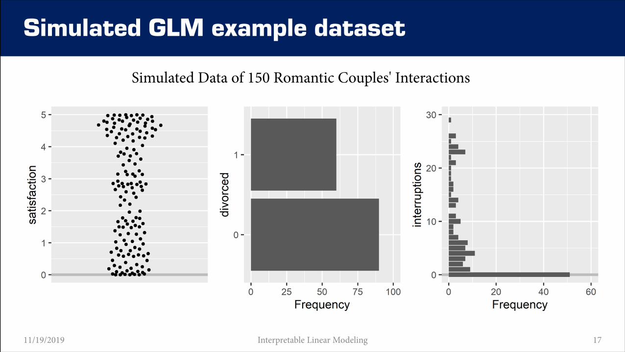
Simulated GLM example dataset

Simulated Data of 150 Romantic Couples' Interactions



divorced ~ 1 + satisfaction


Example of LM for binary data


𝛼𝛼 (Intercept) 0.98 [0.89, 1.07]𝛽𝛽 satisfaction −0.22 [−0.25,−0.19]𝜎𝜎 Residual SD 0.304


𝑦𝑦𝑖𝑖 ~ Binomial(1,𝑝𝑝𝑖𝑖)

logit(𝑝𝑝𝑖𝑖) = 𝛼𝛼 + 𝛽𝛽𝑥𝑥𝑖𝑖divorced ~ 1 + satisfaction

family = binomial(link = "logit")


Example of GLM for binary data


𝛼𝛼 (Intercept) 3.52 [2.45, 4.87]𝛽𝛽 satisfaction −1.78 [−2.40,−1.30]

Deviance = 82.04, Pseudo 𝑅𝑅2 = 0.664

Note: Results are in transformed (i.e., logit) units



interruptions ~ 1 + satisfaction


Example of LM for count data


𝛼𝛼 (Intercept) 17.11 [15.76, 18.45]𝛽𝛽 satisfaction −3.95 [−4.38,−3.52]𝜎𝜎 Residual SD 4.61


𝑦𝑦𝑖𝑖 ~ Poisson(𝜆𝜆𝑖𝑖)

log(𝜆𝜆𝑖𝑖) = 𝛼𝛼 + 𝛽𝛽𝑥𝑥𝑖𝑖interruptions ~ 1 + satisfactionfamily = poisson(link = "log")


Example of GLM for count data


𝛼𝛼 (Intercept) 3.16 [3.08, 3.24]𝛽𝛽 satisfaction −0.77 [−0.83,−0.72]

Deviance = 325.24, Pseudo 𝑅𝑅2 = 0.895

Note: Results are in transformed (i.e., log) units

Multilevel Modeling

• MLM allows (G)LM to handle data points that are dependent/clustered• This is problematic because data within a cluster are likely to be similar• Effects (e.g., intercepts and slopes) may also differ between clusters


What is multilevel modeling?

Person 1

Obs. 1

X

Y

Obs. 2

X

Y

Obs. 3

X

Y

Person 2

Obs. 1

X

Y

Obs. 2

X

Y

Obs. 3

X

Y

Person 3

Obs. 1

X

Y

Obs. 2

X

Y

Obs. 3

X

Y

• One approach would be to estimate effects across all clusters (complete pooling)• But this would require all clusters to be nearly identical, which they may not be

• Another would be to estimate effects for each cluster separately (no pooling)• But this would ignore similarities between clusters and may overfit the data

• The MLM approach tries to have the best of both approaches (partial pooling)• MLM tries to learn the similarities and the differences between clusters• It estimates effects for each individual cluster separately• But these effects are assumed to be drawn from a population of clusters• MLM explicitly models this population and the cluster-specific variation



• MLM comes with several important benefits over single-level models• Improved estimates for repeat sampling• Improved estimates for imbalanced sampling• Estimates of variation across clusters• Avoid averaging and retain variation• Better accuracy and inference!

• Many have argued that "multilevel regression deserves to be the default approach"




𝜇𝜇𝑖𝑖 = 𝛼𝛼CLUSTER[𝑖𝑖]

𝛼𝛼CLUSTER ~ Normal(𝛼𝛼,𝜎𝜎CLUSTER)

• 𝛼𝛼 captures the overall intercept (i.e., the mean of all clusters' intercepts)• 𝛼𝛼CLUSTER 𝑖𝑖 captures each cluster's deviation from the overall intercept• 𝜎𝜎CLUSTER captures how much variability there is across clusters' intercepts• We now have an intercept for every cluster and a "population" of intercepts• The model learns about each cluster's intercept from the population of intercepts

• This pooling within parameters is very helpful for imbalanced sampling


Varying intercepts


Actual MLM example dataset

Real Data of 751 Smiles from 136 Subjects (Girard, Shandar, et al. 2019)


Complete pooling (underfitting)


𝜇𝜇𝑖𝑖 = 𝛼𝛼

smile_int ~ 1


𝛼𝛼 (Intercept) 2.14 [2.10, 2.19]𝜎𝜎 Residual SD 0.66

Deviance = 1495.8


No pooling (overfitting)


𝜇𝜇𝑖𝑖 = 𝛼𝛼PERSON[𝑖𝑖]

smile_int ~ 1 + factor(subject)


𝛼𝛼 1 Intercept for P1 2.14 [1.93, 2.89]𝛼𝛼 2 Intercept for P2 2.17 [1.49, 2.85]… … … …

𝜎𝜎 Residual SD 0.60

Deviance = 1210.10


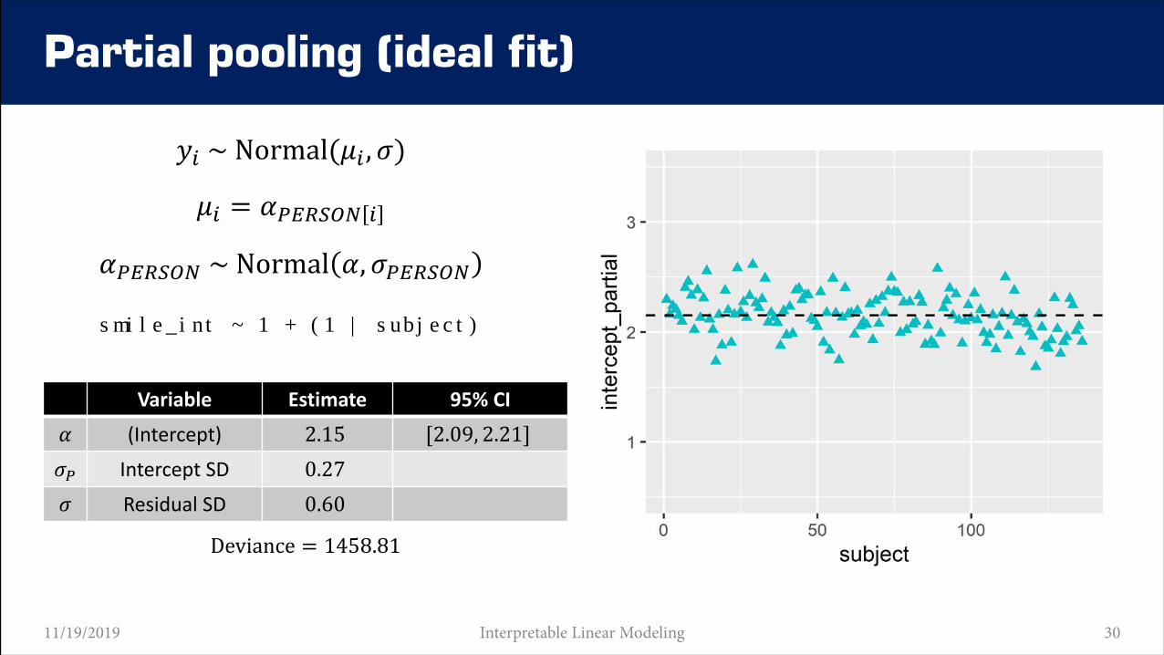
Partial pooling (ideal fit)


𝜇𝜇𝑖𝑖 = 𝛼𝛼𝑃𝑃𝑃𝑃𝑃𝑃𝑃𝑃𝑃𝑃𝑃𝑃 𝑖𝑖

𝛼𝛼𝑃𝑃𝑃𝑃𝑃𝑃𝑃𝑃𝑃𝑃𝑃𝑃 ~ Normal 𝛼𝛼,𝜎𝜎𝑃𝑃𝑃𝑃𝑃𝑃𝑃𝑃𝑃𝑃𝑃𝑃

smile_int ~ 1 + (1 | subject)


𝛼𝛼 (Intercept) 2.15 [2.09, 2.21]𝜎𝜎𝑃𝑃 Intercept SD 0.27𝜎𝜎 Residual SD 0.60

Deviance = 1458.81


Shrinkage in action


𝜇𝜇𝑖𝑖 = 𝛼𝛼CLUSTER 𝑖𝑖 + 𝛽𝛽CLUSTER 𝑖𝑖 𝑥𝑥𝑖𝑖𝛼𝛼CLUSTER𝛽𝛽CLUSTER ~ MVNormal

𝛼𝛼𝛽𝛽, 𝐒𝐒

𝐒𝐒 =𝜎𝜎𝛼𝛼 00 𝜎𝜎𝛽𝛽

𝐑𝐑𝜎𝜎𝛼𝛼 00 𝜎𝜎𝛽𝛽

• We can pool and learn from the covariance between varying intercepts and slopes• We do this with a 2D normal distribution with means 𝛼𝛼 and 𝛽𝛽 and covariance matrix 𝐒𝐒• We build 𝐒𝐒 through matrix multiplication of the variances and correlation matrix 𝐑𝐑• This is more complex but results in even better pooling: within and across parameters


Varying intercepts and slopes


MLM with varying intercepts and slopes


𝜇𝜇𝑖𝑖 = 𝛼𝛼PERSON 𝑖𝑖 + 𝛽𝛽PERSON 𝑖𝑖 𝑥𝑥𝑖𝑖𝛼𝛼PERSON𝛽𝛽PERSON ~ MVNormal

𝛼𝛼𝛽𝛽, 𝐒𝐒

𝐒𝐒 =𝜎𝜎𝛼𝛼 00 𝜎𝜎𝛽𝛽

𝐑𝐑𝜎𝜎𝛼𝛼 00 𝜎𝜎𝛽𝛽

smile_int ~ 1 + amused_sr + (1 + amused_sr| subject)

Deviance = 1458.81


𝛼𝛼 (Intercept) 1.98 [1.91, 2.06]𝛽𝛽 amused_sr 0.12 [0.09, 0.15]𝜎𝜎𝛼𝛼 Intercept SD 0.24 [0.17, 0.32]𝜎𝜎𝛽𝛽 Slope SD 0.04 [0.00, 0.08]

𝐑𝐑 corr 𝜎𝜎𝛼𝛼 ,𝜎𝜎𝛽𝛽 0.30 [−0.69, 0.96]

𝜎𝜎 Residual SD 0.57 [0.54, 0.60]


Depiction of varying intercepts and slopes

Documents

Interpretable Linear Modeling - Piazza