Embed Size (px)
Citation preview
Rec. ITU-R F.1101 1
RECOMMENDATION ITU-R F.1101*
Characteristics of digital fixed wireless systems below about 17 GHz
(Question ITU-R 135/9)
(1994)
The ITU Radiocommunication Assembly,
considering
a) that it is preferable to define certain aspects of the characteristics of digital fixed wireless systems (DFWS) operating below about 17 GHz in order to facilitate system design;
b) that digital fixed wireless system characteristics are determined by the gross bit rate, modulation method, spectrum shaping, interference susceptibility and other relevant factors;
c) that adaptive techniques offer effective countermeasures to adverse propagation conditions and a means of reducing interference in certain circumstances. These techniques are particularly suitable for large bandwidth systems and for systems using complex modulation schemes;
d) that multi-state modulation is an effective method for increasing spectrum utilization efficiency;
e) that when spectrum efficiency is not a major issue, more simple modulation schemes (up to four states) are also suitable for low and medium capacity systems,
recommends
1 that the factors contained in Annex 1 should be taken into consideration in the design of digital fixed wireless systems operating below about 17 GHz.
NOTE 1 – The material contained in this Recommendation is for guidance only. DFWS are not required to have all the features listed herein but can make use of one or several of them, depending on the application for which they are designed.
____________________
* Radiocommunication Study Group 9 made editorial amendments to this Recommendation in 2002 in accordance with Resolution ITU-R 44.
2 Rec. ITU-R F.1101
ANNEX 1
Factors to be considered in the design of digital systems operating below 17 GHz
1 Categorization of digital fixed wireless systems
It seems advisable to subdivide digital fixed wireless systems into the following categories:
– low capacity fixed wireless systems for the transmission of digital signals with gross bit rates up to and including 10 Mbit/s;
– medium capacity fixed wireless systems for the transmission of digital signals with gross bit rates ranging from 10 Mbit/s up to about 100 Mbit/s;
– high capacity fixed wireless systems for the transmission of digital signals with gross bit rates greater than 100 Mbit/s.
2 Predominant propagation factor
Error performance and availability are representative parameters featuring digital fixed wireless systems. As far as the propagation path characteristics are concerned, rain attenuation predominates at frequencies above about 17 GHz, while multipath distortion predominates at frequencies below about 10 GHz.
For this reason, digital fixed wireless systems should be mainly designed in terms of unavailability at frequencies above 17 GHz and error performance at frequencies below about 10 GHz, while in the range 10-17 GHz both objectives should be considered.
3 Modulation and coding techniques
Coding and modulation techniques used are of particular concern to the fixed wireless system. Coding consists of a transformation of the format of the signals in the alphabet to take account of the methods of synchronization, introduction of redundancy in accordance with the error-control and/or correction system (forward error correction), spectrum shaping and to meet the requirements of interfacing with the transmission medium or channel. Modulation consists of transferring information in the baseband signal onto an RF carrier. In general, this is achieved by a single change or combined changes in the phase, frequency or amplitude of the RF carrier for radio-frequency transmission.
3.1 Comparison of some methods of modulation
Different modulation techniques may be compared theoretically on the basis of their Nyquist bandwidth and the normalized carrier-to-noise ratio. The real carrier-to-noise ratio (allowing for all imperfections) needs to be considered in order to define real systems.
Detailed information on this subject is given in Appendix 1.
Rec. ITU-R F.1101 3
3.2 Modulation methods
A suitable modulation method is selected by taking into account the system requirements. For instance, if spectrum efficiency is not a major issue and/or high interference tolerance is important, a simple modulation method should be used. The features of simple modulation methods are:
– easy implementation in all frequency bands,
– robustness against propagation effects,
– high tolerance against all kinds of interferences,
– high system gain characteristics.
On the other hand, a multi-state modulation method improves spectral efficiency on a route. Typical applications for multi-state modulation methods are high capacity trunk, junction and access networks.
Careful design of the multi-state constellation for QAM schemes might achieve some system gain against non-linear distortion while retaining a fairly simple implementation.
Consideration of the carrier-to-noise requirement for the same BER when changing from 16-state to 512-state modulation, for example, shows the need for significant increases in peak power, average power and peak-to-average power ratio. This places more stringent requirements on the high power amplifier, and will in many cases require the use of linearization measures, such as pre-distortion.
3.3 Data coding and error correction
In order to improve the tolerance of the modem to various sources of C/N impairment, data coding and error correction techniques may be used for radio systems employing multi-state modulation schemes.
The introduction of forward error correction coding is also useful for reducing the residual bit errors. Various types of codes are employed in multi-state modulation schemes. It should be noted that code efficiency is required for band-limited digital radio applications.
3.3.1 Forward error correction
There are several types of error correction techniques. One involves the use of error correction codes such as block codes and convolutional codes, where redundant parity bits are inserted into the time domain.
In the conventional method of forward error correction, the incoming data are passed through an encoder which adds redundant parity bits. The combined set of information and parity bits are then modulated and transmitted. Upon reception, the demodulated data are subjected to a symbol-by-symbol hard decision on each demodulated symbol. The demodulated symbols are then decoded to extract the information bits with appropriate corrections as governed by parity bits.
3.3.2 Coded modulation
This method is a technique that combines coding and modulation which would have been done independently in the conventional method. Redundant bits are inserted in multi-state numbers of transmitted signal constellations (see Appendix 1). This is known as coded modulation.
4 Rec. ITU-R F.1101
Representative examples of coded modulation are block coded modulation (BCM), trellis coded modulation (TCM) and multi-level coded modulation (MLC or MLCM). In BCM, levels are coded by block codes whereas TCM uses only convolutional codes. On the other hand, different codes can be used for each coded level in MLCM, so MLCM can be seen as a general concept that includes BCM and to some extent TCM. These schemes require added receiver complexity in the form of a maximum likelihood decoder with soft decision. Tables 1a and 1b provide indications of expected performances.
A technique similar to TCM is the partial response, sometimes called a duo-binary or correlative signalling system. A controlled amount of intersymbol interference, or redundancy is introduced into the channel. Hence, the signal constellation is expanded without increasing the transmitted data bandwidth. There are various methods utilizing this redundancy to detect and then correct errors to improve performance. This process is called “ambiguity zone detection” or AZD.
Additional information on BCM, TCM, MLCM and partial response with AZD is given in Appendix 2.
4 Radio spectrum utilization efficiency
Radio spectrum utilization efficiency is an important factor to be considered in the design of digital fixed wireless systems and it is determined by the “information transferred over a distance” in relation to the frequency bandwidth utilization, the geometric (geographic) spatial utilization and the time denied to other potential users. The measure of utilization (U) is given by the product:
U = BRF · S · T
where:
BRF : radio-frequency bandwidth occupied
S : geometric space occupied (usually area for fixed wireless systems)
T : time.
The utilization efficiency, E, for a system operating continuously in time is expressed by:
E = 2 · N · B
BRF · S
where:
N : total number of “go” and “return” channels in the radio band BRF
B : channel gross bit rate.
In the case of single high or medium capacity multi-channel long-haul routes, in which spurious emissions are adequately controlled and the dimensions of space and time can be ignored, the radio-frequency spectrum utilization efficiency reduces to a bandwidth utilization efficiency EB, given by:
EB = 2 · N · B
BRF
where N includes both polarizations on the route.
Rec. ITU-R F.1101 5
It can be seen that the use of multi-state modulation methods increases the bandwidth utilization efficiency in this case by an increase of B.
Detailed information on this subject is given in Recommendation ITU-R SM.1046.
5 Technical basis of co-channel and alternated arrangements for digital fixed wireless systems
5.1 Parameters affecting co-channel and alternated radio-frequency arrangement
This subject is described in recommends 2 of Recommendation ITU-R F.746.
5.2 Shaping filter requirements
Channel shaping filtering may, in principle, be performed at baseband, intermediate or radio frequencies. It must be designed so as to control the overlap of adjacent spectra.
Generally, transmitter and receiver filters, used to control adjacent frequency channel interference and to restrict the receiver noise bandwidth, are designed to have a Nyquist raised cosine roll-off shaping, which theoretically does not give intersymbol interference.
The roll-off factor, α, of such a Nyquist filter may be chosen taking into account that, for a theoretical no-interference condition, the following relation applies:
α ≤ x − 1
where x is the width of the radio-frequency channel normalized with respect to the symbol frequency.
The balance between allowable interference level for the chosen modulation format, the increase of peak-to-average carrier power requirements (as reported in Appendix 1) and the reduction of the timing margin for a no intersymbol interference condition, governs practical implementations.
6 Technical bases of performance and availability objectives for digital fixed wireless systems employing multi-state modulation
In order to efficiently utilize the limited resource of radio-frequency spectrum, multi-state modulation schemes may be employed for high capacity digital fixed wireless systems. As the number of modulation states increases, the performance of the modem and the radio system is impaired by several factors. These are:
– the stability of carrier and clock synchronization circuits,
– amplitude distortion due to the transmission path,
– distortion caused by saturation of the high power amplifier,
– interference from other systems (adjacent channels, satellite, adjacent route, etc.),
– multipath fading.
6 Rec. ITU-R F.1101
It is therefore necessary to consider the mechanisms causing the impairments and devise the appropriate countermeasures. The following topics should be studied. Fuller details may be found in Recommendation ITU-R F.1093.
6.1 Factors affecting error performance
Waveform distortion and interference during multipath fading are dominant factors in determining the severely errored seconds in digital fixed wireless systems operating below about 10 GHz. Both factors have to be taken into account when designing digital radio systems.
The following gives a brief introduction to many methods used to estimate the effects of propagation on the performance of digital radio.
6.2 Susceptibility to multipath fading
6.2.1 System signature
Digital fixed wireless systems are particularly affected by the frequency selective nature of multipath fading. Fading effects on a radio may be characterized by a “system signature”. Numerical methods with computer simulation could be useful for signature computation. A “system signature” is basically a static measure of the susceptibility of a particular equipment to a two ray model of the multipath channel in both minimum phase and non-minimum phase conditions. It is being used as a basis for equipment comparisons.
An important aspect of multipath fading is its dynamic nature. Therefore dynamic tests should be performed to assure satisfactory equipment performance. Dynamic multipath fading may be simulated in the laboratory by a dynamic simulator capable of simulating the time sequences of multipath fading. These tests will allow the optimization of synchronization and equalizer coefficient adaptation circuits.
Further studies are needed to define optimum test sequences for dynamic testing.
6.2.2 Normalized signature
Another approach to the use of waveform factor is the use of a normalized signature constant. This constant can be derived from theoretical signature and/or measurements and can be used to compare modulation methods and countermeasures such as equalizers and diversity.
6.3 Countermeasures to multipath fading
In order to mitigate the propagation impairments, various countermeasures such as space diversity, frequency diversity, angle diversity and adaptive equalizers in the time and frequency domains are described in Recommendation ITU-R F.752.
6.3.1 Equalizers
Technological advances in equalization techniques have been very effective in minimizing the effects of anomalous propagation on digital radio performance. As the number of modulation states increases, the radio system becomes more vulnerable to multipath fading. Various types of adaptive
Rec. ITU-R F.1101 7
equalizers are currently in use for digital fixed wireless systems and are implemented at intermediate and/or at baseband frequencies. Among these equalizers, decision-feedback equalizers and linear transversal equalizers are in common use. A powerful solution is represented by the so-called fractionally-spaced linear transversal equalizer (FSLTE), in which the signal is sampled several (at least two) times within one symbol period. Such a solution shows a better performance/complexity ratio, together with a lower sensitivity to timing phase (when the central tap is not fixed). Moreover, FSLTEs, implemented with a two samples/symbol sampling, combine “naturally” with receiver over-sampling digital filtering (shaping filters), and with simplified minimum mean square error (MMSE) algorithms for timing recovery.
For optimum performance, the dynamic convergence of FSLTEs should be accomplished by means of “blind” algorithms (as with synchronous LTE), combined with the recursive updating of tap coefficients, reference-tap position and timing phase, for both initial convergence and channel tracking.
6.3.2 Multi-carrier transmission
A multi-carrier transmission method in which the symbol rate can be decreased in proportion to the number of carriers of the multi-carrier system is also an effective technique to mitigate induced waveform distortion. The waveform factor may be used to assess the relationship between symbol rate and modulation method for a particular outage budget. This relationship is given in a pictorial form in Recommendation ITU-R F.1093, from which the maximum symbol rate that may be transmitted for a given modulation scheme may be established, once an outage budget is specified.
If the gross data rate to be transmitted exceeds the corresponding value calculated from the symbol rate in the above method, then the use of multi-carrier techniques may be necessary. It is also possible to determine the number of carriers needed in the multi-carrier case.
In general, the use of a multi-carrier method requires the development of higher linearity power amplifiers and the optimization of sub-carrier spacing to avoid intermodulation distortions and intra-system interference produced by adjacent carriers of the same multi-carrier system.
6.4 Susceptibility to interference and noise
Consideration of various kinds of interferers arising in a radio system is important in the choice of a modulation scheme and the associated hardware needed.
Adjacent cross-polarized channel interference (ACI) may become one of the main factors in the design of radio systems. The value of ACI is dependent upon antenna cross-polar discrimination (XPD). As the XPD degrades during fading, ACI may become crucial in noise budget calculations of the radio system. In order to minimize the detrimental effects of ACI on 64-QAM and other multi-state modulation methods, improved antenna XPD or a smaller roll-off factor pulse shaping filter may be necessary.
8 Rec. ITU-R F.1101
The factor, W, also gives a measure of the received carrier power level required to maintain a given level of degradation from fixed broadband interference, as the symbol rate is varied. However, when interference is between a number of similar transmissions, all with symbol rates, occupied bandwidth and relative spectral positions reduced in the same ratio, the degrading effects can only be maintained at a constant level by introducing some means of compensatory interference reduction – for example, improved antenna discrimination (at network nodes), improved XPD, or larger RF channel spacings (on a route). If this last expedient is adopted, improvement in spectrum utilization efficiency on a route is no longer inversely proportional to symbol rate. The magnitude of the interference reduction required is proportional to the change in the value of W and to the ratio of symbol rates.
Various interference factors introducing ground scattering become more significant in multi-state modulation systems (see Recommendation ITU-R P.530).
The outage probability due to thermal noise and interference is given by (see Recommen-dation ITU-R P.530):
Pn = am × 10−A/10 single antenna reception
= (aSD / (1 − ρs)) × 10−A/5 space diversity reception
where:
A : system flat fade margin (dB)
am, aSD : constants determined by frequency, path length and path parameters
ρs: spatial coefficient between two antennas.
Suppose that the outage probabilities due to waveform distortion and interference noise are represented as Pd and Pn, respectively. The total outage probability (P0) may be evaluated from the composite fade margin concept, for example:
P0 = Pd + Pn single antennna reception
= Pd + Pn 2 space diversity reception
Where digital fixed wireless systems share the same frequency band with FDM-FM systems in dense networks, FM co-channel interference may be excessive without the use of interference cancellers.
6.5 Countermeasures to interference
6.5.1 Automatic transmit power control (ATPC)
Automatic regulation of the transmitted power of digital fixed wireless systems can be used, in particular, to reduce interference between channels on the same route and between channels radiating from the same system node. This reduction of interference is of value in helping to achieve optimum use of digital fixed wireless systems in a telecommunications network, particularly by:
– increasing the capacity of a system node; a reduced interference power permits a reduction in angular separation between adjacent radial routes;
Rec. ITU-R F.1101 9
– reducing interference from a digital channel into an adjacent analogue channel thus easing compatibility problems in shared bands;
– reducing the digital-to-digital interference between hops which re-use the same frequency.
ATPC is a technique in which the output power of a microwave transmitter is automatically varied in accordance with path conditions. In normal path conditions, the ATPC maintains the transmitter output power at a reduced level. Fades are detected by the far-end receiver and the up-stream transmitter is commanded to increase power via overhead bits.
The full advantages of ATPC are only realized if the power-control signal is closely attuned to error performance and if fading characteristics are taken into account. This means that attention must be paid to possible increases in bit errors as power is increased which causes transmitter linearity to degrade and spill-over into adjacent channels to increase. Attention must also be paid to the partial correlation between AGC signal level, digital signal distortion and interference power-density distribution during multipath fading events.
6.5.2 Cross-polar interference cancellers (XPICs)
Co-channel frequency re-use can be seriously affected by co-frequency cross-polarized interference arising from low XPD values that may occur during periods of multipath fading. The development of antennas with improved XPD characteristics about the boresight may in some circumstances provide co-channel frequency re-use operation. Where additional reduction of cross-polar interference is required, an adaptive canceller (XPIC) may be used in such situations to cancel a cross-polar interference signal from an orthogonal polarized signal.
The XPIC takes samples of the interfering signals, which are available in the cross-polarized channel, and feeds them through complex coupling networks to the desired channel to cancel the interference. The control of the added signal and the compensation of the interference can take place at RF, IF or baseband levels. Transversal filter structures are also used for XPICs to compensate effectively a cross-polar interference signal.
With higher multi-state modulation, such as 256-QAM, a highly precise interference canceller is required to provide adequate equalization performance. Propagation experiments have shown that receiving systems equipped with an XPIC lead to considerably reduced outage times at a BER of 10−3.
6.6 Repeater spacing
Rain attenuation progressively restricts the repeater spacings in digital fixed wireless systems operating above 10 GHz. The degree of restriction depends on frequency and rain rate. Under such circumstances the multipath fading occurrence probability becomes less significant (see Rec-ommendation ITU-R P.530).
10 Rec. ITU-R F.1101
APPENDIX 1
TO ANNEX 1
Comparison of some methods of modulation
Different modulation techniques may be compared on the basis of their Nyquist bandwidth and BER versus carrier-to-noise ratio behaviours.
Since noise power is limited by the actual channel bandwidth used, it is wise to define a “normalized noise bandwidth” in order to compare different modulation and different implementations of the same modulation.
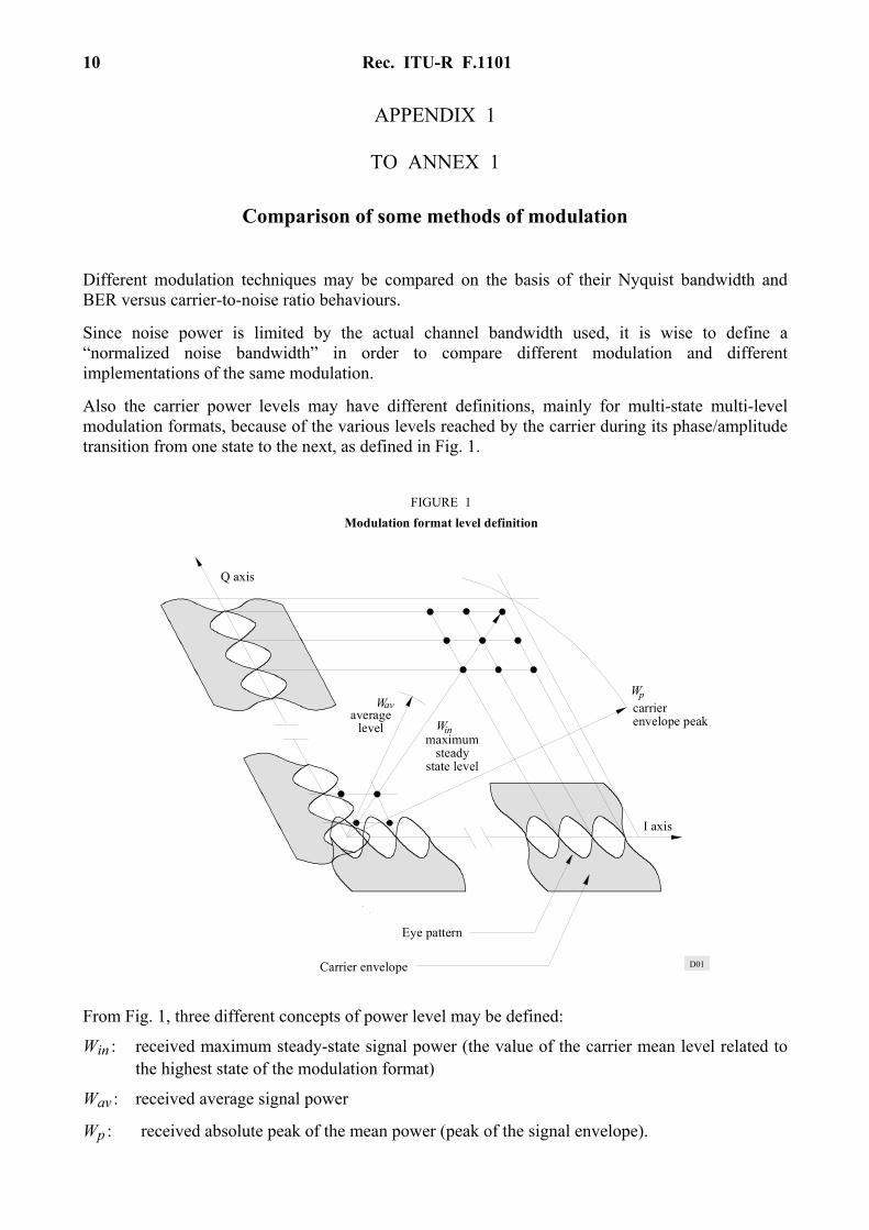
Also the carrier power levels may have different definitions, mainly for multi-state multi-level modulation formats, because of the various levels reached by the carrier during its phase/amplitude transition from one state to the next, as defined in Fig. 1.
D01
Wpcarrierenvelope peak
Wavaverage
level
Q axis
Eye pattern
Carrier envelope
Winmaximum
steadystate level
I axis
FIGURE 1Modulation format level definition
From Fig. 1, three different concepts of power level may be defined:
Win : received maximum steady-state signal power (the value of the carrier mean level related to the highest state of the modulation format)
Wav : received average signal power
Wp : received absolute peak of the mean power (peak of the signal envelope).
Rec. ITU-R F.1101 11
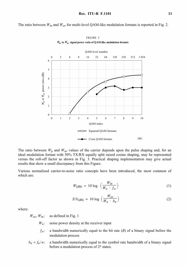
The ratio between Win and Wav for multi-level QAM-like modulation formats is reported in Fig. 2.
0 1 2 3 4 5 6 7 8 9 10
0 2 4 8 16 32 64 128 256 512 1 024
1
2
3
4
5
6
0
D02
W
to W
p
ower
ratio
(dB)
inav
QAM index
QAM level number
FIGURE 2W to W signal power ratio of QAM-like modulation formatsin av
Squared QAM formats
Cross QAM formats
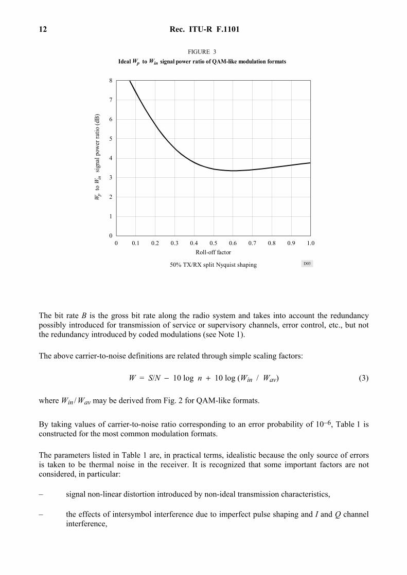
The ratio between Wp and Wav values of the carrier depends upon the pulse shaping and, for an ideal modulation format with 50% TX/RX equally split raised cosine shaping, may be represented versus the roll-off factor as shown in Fig. 3. Practical shaping implementation may give actual results that show a small discrepancy from this Figure.
Various normalized carrier-to-noise ratio concepts have been introduced, the most common of which are:
W(dB) = 10 log Win
Wn · ƒn (1)
S/N(dB) = 10 log Wav
Wn · bn (2)
where:
Wav, Win : as defined in Fig. 1
Wn : noise power density at the receiver input
ƒn : a bandwidth numerically equal to the bit rate (B) of a binary signal before the modulation process
bn = fn / n : a bandwidth numerically equal to the symbol rate bandwidth of a binary signal before a modulation process of 2n states.
12 Rec. ITU-R F.1101
8
7
6
5
4
3
2
1
00 0.1 0.2 0.3 0.4 0.5 0.6 0.7 0.8 0.9 1.0
D03
W
to W
si
gnal
pow
er ra
tio (d
B)p
in
Roll-off factor
FIGURE 3Ideal W to W signal power ratio of QAM-like modulation formatsp in
50% TX/RX split Nyquist shaping
The bit rate B is the gross bit rate along the radio system and takes into account the redundancy possibly introduced for transmission of service or supervisory channels, error control, etc., but not the redundancy introduced by coded modulations (see Note 1).
The above carrier-to-noise definitions are related through simple scaling factors:
W = S/N − 10 log n + 10 log (Win / Wav) (3)
where Win / Wav may be derived from Fig. 2 for QAM-like formats.
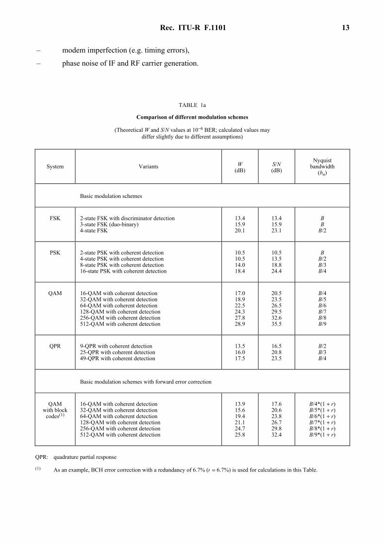
By taking values of carrier-to-noise ratio corresponding to an error probability of 10−6, Table 1 is constructed for the most common modulation formats.
The parameters listed in Table 1 are, in practical terms, idealistic because the only source of errors is taken to be thermal noise in the receiver. It is recognized that some important factors are not considered, in particular:
– signal non-linear distortion introduced by non-ideal transmission characteristics,
– the effects of intersymbol interference due to imperfect pulse shaping and I and Q channel interference,
Rec. ITU-R F.1101 13
– modem imperfection (e.g. timing errors),
– phase noise of IF and RF carrier generation.
TABLE 1a
Comparison of different modulation schemes
(Theoretical W and S/N values at 10−6 BER; calculated values may differ slightly due to different assumptions)
System
Variants W
(dB) S/N (dB)
Nyquist bandwidth
(bn)
Basic modulation schemes
FSK 2-state FSK with discriminator detection 3-state FSK (duo-binary) 4-state FSK
13.4 15.9 20.1
13.4 15.9 23.1
B B
B/2
PSK
2-state PSK with coherent detection 4-state PSK with coherent detection 8-state PSK with coherent detection 16-state PSK with coherent detection
10.5 10.5 14.0 18.4
10.5 13.5 18.8 24.4
B B/2 B/3 B/4
QAM 16-QAM with coherent detection 32-QAM with coherent detection 64-QAM with coherent detection 128-QAM with coherent detection 256-QAM with coherent detection 512-QAM with coherent detection
17.0 18.9 22.5 24.3 27.8 28.9
20.5 23.5 26.5 29.5 32.6 35.5
B/4 B/5 B/6 B/7 B/8 B/9
QPR 9-QPR with coherent detection 25-QPR with coherent detection 49-QPR with coherent detection
13.5 16.0 17.5
16.5 20.8 23.5
B/2 B/3 B/4
Basic modulation schemes with forward error correction
QAM with block
codes(1)
16-QAM with coherent detection 32-QAM with coherent detection 64-QAM with coherent detection 128-QAM with coherent detection 256-QAM with coherent detection 512-QAM with coherent detection
13.9 15.6 19.4 21.1 24.7 25.8
17.6 20.6 23.8 26.7 29.8 32.4
B/4*(1 + r) B/5*(1 + r) B/6*(1 + r) B/7*(1 + r) B/8*(1 + r) B/9*(1 + r)
QPR: quadrature partial response
(1) As an example, BCH error correction with a redundancy of 6.7% (r = 6.7%) is used for calculations in this Table.
14 Rec. ITU-R F.1101
TABLE 1b
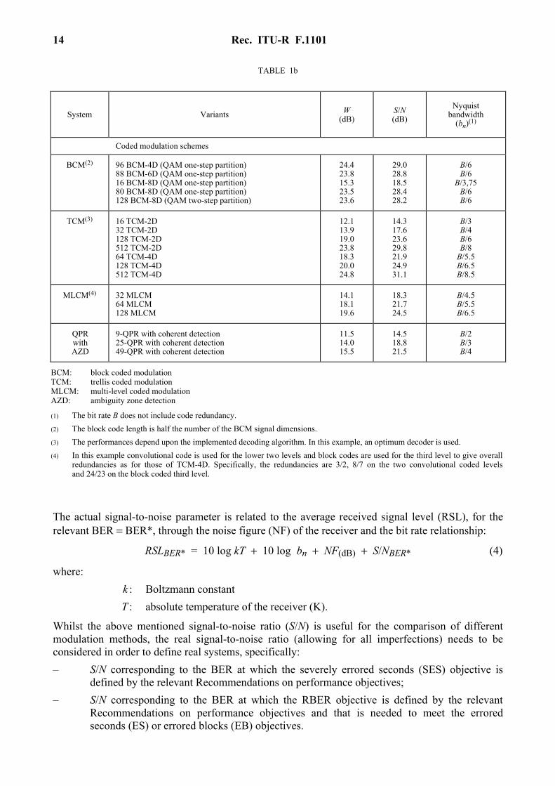
The actual signal-to-noise parameter is related to the average received signal level (RSL), for the relevant BER = BER*, through the noise figure (NF) of the receiver and the bit rate relationship:
RSLBER* = 10 log kT + 10 log bn + NF(dB) + S/NBER* (4)
where: k : Boltzmann constant T : absolute temperature of the receiver (K).
Whilst the above mentioned signal-to-noise ratio (S/N) is useful for the comparison of different modulation methods, the real signal-to-noise ratio (allowing for all imperfections) needs to be considered in order to define real systems, specifically: – S/N corresponding to the BER at which the severely errored seconds (SES) objective is
defined by the relevant Recommendations on performance objectives; – S/N corresponding to the BER at which the RBER objective is defined by the relevant
Recommendations on performance objectives and that is needed to meet the errored seconds (ES) or errored blocks (EB) objectives.
System
Variants W
(dB) S/N (dB)
Nyquist bandwidth
(bn)(1)
Coded modulation schemes
BCM(2) 96 BCM-4D (QAM one-step partition) 88 BCM-6D (QAM one-step partition) 16 BCM-8D (QAM one-step partition) 80 BCM-8D (QAM one-step partition) 128 BCM-8D (QAM two-step partition)
24.4 23.8 15.3 23.5 23.6
29.0 28.8 18.5 28.4 28.2
B/6 B/6
B/3,75 B/6 B/6
TCM(3) 16 TCM-2D 32 TCM-2D 128 TCM-2D 512 TCM-2D 64 TCM-4D 128 TCM-4D 512 TCM-4D
12.1 13.9 19.0 23.8 18.3 20.0 24.8
14.3 17.6 23.6 29.8 21.9 24.9 31.1
B/3 B/4 B/6 B/8
B/5.5 B/6.5 B/8.5
MLCM(4) 32 MLCM 64 MLCM 128 MLCM
14.1 18.1 19.6
18.3 21.7 24.5
B/4.5 B/5.5 B/6.5
QPR with AZD
9-QPR with coherent detection 25-QPR with coherent detection 49-QPR with coherent detection
11.5 14.0 15.5
14.5 18.8 21.5
B/2 B/3 B/4
BCM: block coded modulation TCM: trellis coded modulation MLCM: multi-level coded modulation AZD: ambiguity zone detection
(1) The bit rate B does not include code redundancy. (2) The block code length is half the number of the BCM signal dimensions. (3) The performances depend upon the implemented decoding algorithm. In this example, an optimum decoder is used. (4) In this example convolutional code is used for the lower two levels and block codes are used for the third level to give overall
redundancies as for those of TCM-4D. Specifically, the redundancies are 3/2, 8/7 on the two convolutional coded levels and 24/23 on the block coded third level.
Rec. ITU-R F.1101 15
The Nyquist bandwidth (bn) occupied by the modulated signal can also be used in comparing various modulation schemes. However this does not generally indicate the radio-frequency channel bandwidth that in practice must be allotted to a digitally modulated signal. This channel bandwidth is, in principle, a trade-off between the choice of modulation, inter-channel interference and network constraints and, in practice, is provided by the relevant ITU-R Recommendation on radio-frequency channel arrangements. It is expected to vary in the range 1.2 bn to 2 bn for various systems, except in the case of QPR which can transmit in a bandwidth equal to that of the Nyquist bandwidth (1 × bn).
NOTE 1 – In coded modulation methods using a multi-state modulation format, redundant bits are inserted increasing the bit rate by a factor:
(n + 1) / (n + z)
where z is a factor depending on the adopted coded modulation (z < 1).
In the meantime, the number of states are increased from 2n (that should have been used for uncoded modulation) to 2n+1.
In this way, the actual symbol rate (bn) transmitted (related to the band occupancy) will become:
bn = B ·
n + 1n + z
n + 1 = B
n + z
APPENDIX 2
TO ANNEX 1
Coded modulation techniques
1 Block coded modulation
BCM is a technique for generating multi-dimensional signal constellations which have both large distances (i.e. good error performance) and also regular structures allowing an efficient parallel demodulation architecture called staged decoding. It obtains a sub-set of the Cartesian product of a number of elementary (i.e. low dimensional) signal sets by itself. The staged construction allows demodulation algorithms based on projection of the signal set into lower-dimensional, lower-size constellations. These algorithms lend themselves quite naturally to a pipelined architecture.
16 Rec. ITU-R F.1101
Multi-dimensional signals with large distances can be generated by combining algebraic codes of increasing Hamming distance with nested signal constellations of decreasing Euclidian distance.
Compared to TCM (see § 2), BCM schemes give smaller coding gains. However BCM often requires a lower demodulator complexity than TCM with the same performance and it lends itself to a parallel demodulator architecture, which might prove to be a bonus if high processing speeds are necessary.
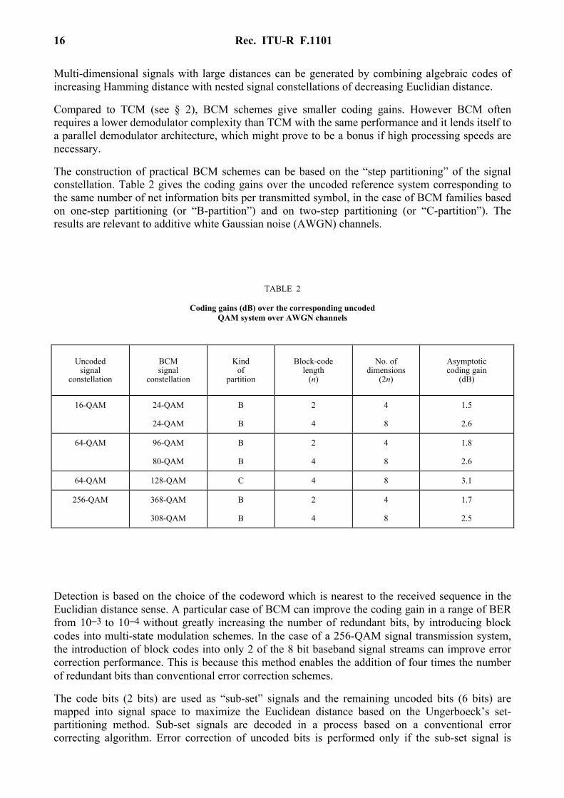
The construction of practical BCM schemes can be based on the “step partitioning” of the signal constellation. Table 2 gives the coding gains over the uncoded reference system corresponding to the same number of net information bits per transmitted symbol, in the case of BCM families based on one-step partitioning (or “B-partition”) and on two-step partitioning (or “C-partition”). The results are relevant to additive white Gaussian noise (AWGN) channels.
TABLE 2
Coding gains (dB) over the corresponding uncoded QAM system over AWGN channels
Detection is based on the choice of the codeword which is nearest to the received sequence in the Euclidian distance sense. A particular case of BCM can improve the coding gain in a range of BER from 10−3 to 10−4 without greatly increasing the number of redundant bits, by introducing block codes into multi-state modulation schemes. In the case of a 256-QAM signal transmission system, the introduction of block codes into only 2 of the 8 bit baseband signal streams can improve error correction performance. This is because this method enables the addition of four times the number of redundant bits than conventional error correction schemes.
The code bits (2 bits) are used as “sub-set” signals and the remaining uncoded bits (6 bits) are mapped into signal space to maximize the Euclidean distance based on the Ungerboeck’s set-partitioning method. Sub-set signals are decoded in a process based on a conventional error correcting algorithm. Error correction of uncoded bits is performed only if the sub-set signal is
Uncoded signal
constellation
BCM signal
constellation
Kind of
partition
Block-code length
(n)
No. of dimensions
(2n)
Asymptotic coding gain
(dB)
16-QAM 24-QAM
24-QAM
B
B
2
4
4
8
1.5
2.6
64-QAM 96-QAM
80-QAM
B
B
2
4
4
8
1.8
2.6
64-QAM 128-QAM C 4 8 3.1
256-QAM 368-QAM
308-QAM
B
B
2
4
4
8
1.7
2.5
Rec. ITU-R F.1101 17
corrected. At the specific time-slot, the uncoded bits are decoded by selecting a signal point that is located nearest to the received signal point from the coded sub-set signals using soft-decision information.
When the BCH (31,11) code is employed as the above-mentioned block code modulation, a coding gain of about 5 dB can be obtained at a BER of 10−4. The application of block code modulation has led to a coding gain of about 5 dB at a BER of 10−4.
2 Trellis coded modulation
Trellis coded modulations are explained as generalized convolutional coding with non-binary signals optimized to achieve large “free Euclidian distance”, dE, among sequences of transmitted symbols. As a result, a lower signal-to-noise ratio or a smaller bandwidth is required to transmit data at a given rate and error probability.
To achieve this, a redundant signal alphabet is used. It is obtained by convolutionally encoding k out of n information bits to be transmitted at a certain time. The convolutional code has rate k/(k + 1), and adds 1 bit redundancy. In the symbol-mapping procedure that follows the convolutional encoder, the encoder bits determine the sub-set (or “sub-modulation”) to which the transmitted symbol belongs, and the uncoded bits determine a particular signal point in that sub-set. The mapping procedure is also called “set-partitioning” and has the purpose of increasing the minimum distance dE among the symbols.
The optimum receiver for the trellis coded sequence requires a maximum likelihood sequence estimation (MLSE) that can be implemented as a Viterbi algorithm.
Since the redundancy of coding in the time domain, as used in serial FEC, is replaced by a “spatial” redundancy, the cost of coding gain is not an increase of the necessary transmission bandwidth, but a higher modulation complexity.
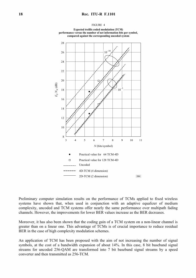
Another advantage of TCMs is their higher flexibility with respect to serial coding, because of the possibility of increasing the constellation efficiency by 1 bit/symbol (in the case of 4-D codes). On an additive white Gaussian noise channel, the coding gain over an uncoded reference system is represented in Fig. 4, considering the case of a rate 2/3, 8 sub-set encoder and 3 bit soft decision Viterbi decoder.
The coding gain over the uncoded reference system (corresponding to the same number of net information bits per transmitted symbol) is about 2 dB at BER = 10−3 and about 4 dB at BER = 10−10, in the case of 2-D codes. In the case of 4-D codes, such gains are 1.8 dB and 3.5 dB, respectively. Some practical values have also been reported (see Fig. 4).
18 Rec. ITU-R F.1101
10–10
24
22
20
26
18
16
14
12
10
83 4 5 6 7 8 9 10 11
28
10–3
E /N
(d
B)
b0
N (bits/symbol)
Practical value for 164 TCM-4D
Practical value for 128 TCM-4DUncoded
4D-TCM (4 dimension)
2D-TCM (2 dimension) D04
FIGURE 4Expected treillis coded modulation (TCM)
performance versus the number of net information bits per symbol,compared against the corresponding uncoded system
Preliminary computer simulation results on the performance of TCMs applied to fixed wireless systems have shown that, when used in conjunction with an adaptive equalizer of medium complexity, uncoded and TCM systems offer nearly the same performance over multipath fading channels. However, the improvements for lower BER values increase as the BER decreases.
Moreover, it has also been shown that the coding gain of a TCM system on a non-linear channel is greater than on a linear one. This advantage of TCMs is of crucial importance to reduce residual BER in the case of high complexity modulation schemes.
An application of TCM has been proposed with the aim of not increasing the number of signal symbols, at the cost of a bandwidth expansion of about 14%. In this case, 8 bit baseband signal streams for uncoded 256-QAM are transformed into 7 bit baseband signal streams by a speed converter and then transmitted as 256-TCM.
Rec. ITU-R F.1101 19
3 Multi-level coded modulation
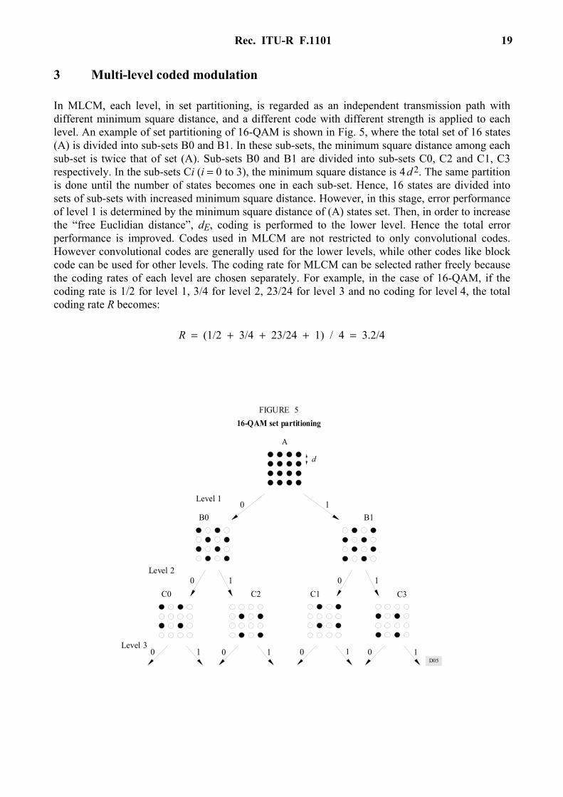
In MLCM, each level, in set partitioning, is regarded as an independent transmission path with different minimum square distance, and a different code with different strength is applied to each level. An example of set partitioning of 16-QAM is shown in Fig. 5, where the total set of 16 states (A) is divided into sub-sets B0 and B1. In these sub-sets, the minimum square distance among each sub-set is twice that of set (A). Sub-sets B0 and B1 are divided into sub-sets C0, C2 and C1, C3 respectively. In the sub-sets Ci (i = 0 to 3), the minimum square distance is 4 d 2. The same partition is done until the number of states becomes one in each sub-set. Hence, 16 states are divided into sets of sub-sets with increased minimum square distance. However, in this stage, error performance of level 1 is determined by the minimum square distance of (A) states set. Then, in order to increase the “free Euclidian distance”, dE, coding is performed to the lower level. Hence the total error performance is improved. Codes used in MLCM are not restricted to only convolutional codes. However convolutional codes are generally used for the lower levels, while other codes like block code can be used for other levels. The coding rate for MLCM can be selected rather freely because the coding rates of each level are chosen separately. For example, in the case of 16-QAM, if the coding rate is 1/2 for level 1, 3/4 for level 2, 23/24 for level 3 and no coding for level 4, the total coding rate R becomes:
R = (1/2 + 3/4 + 23/24 + 1) / 4 = 3.2/4
C0 C2 C1 C3
B0 B1
A
d
0 1
0 1 0 1
0 1 0 1 0 1 0 1D05
Level 1
Level 2
Level 3
FIGURE 516-QAM set partitioning
20 Rec. ITU-R F.1101
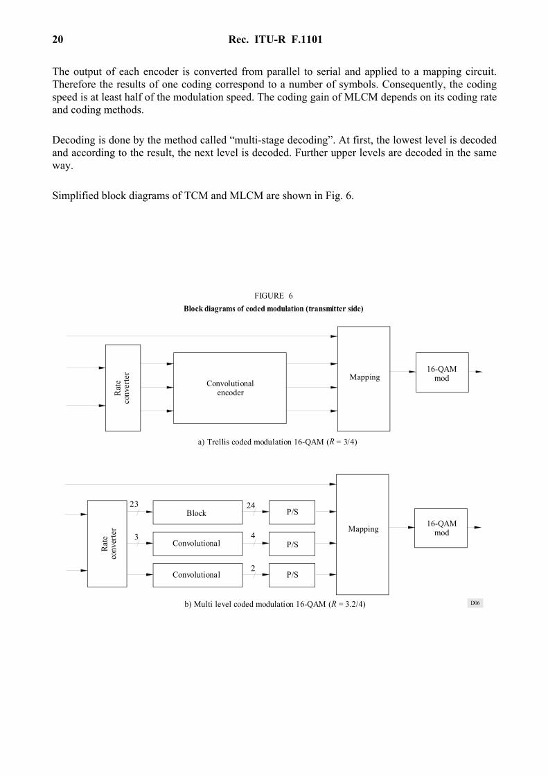
The output of each encoder is converted from parallel to serial and applied to a mapping circuit. Therefore the results of one coding correspond to a number of symbols. Consequently, the coding speed is at least half of the modulation speed. The coding gain of MLCM depends on its coding rate and coding methods.
Decoding is done by the method called “multi-stage decoding”. At first, the lowest level is decoded and according to the result, the next level is decoded. Further upper levels are decoded in the same way.
Simplified block diagrams of TCM and MLCM are shown in Fig. 6.
D06
23
3
24
4
2
Mapping 16-QAMmod
Block
Convolutional
Convolutional
Rate
conv
erte
r
P/S
P/S
P/S
Convolutionalencoder
Mapping
b) Multi level coded modulation 16-QAM (R = 3.2/4)
a) Trellis coded modulation 16-QAM (R = 3/4)
FIGURE 6Block diagrams of coded modulation (transmitter side)
16-QAMmod
Rat
eco
nver
ter
Rec. ITU-R F.1101 21
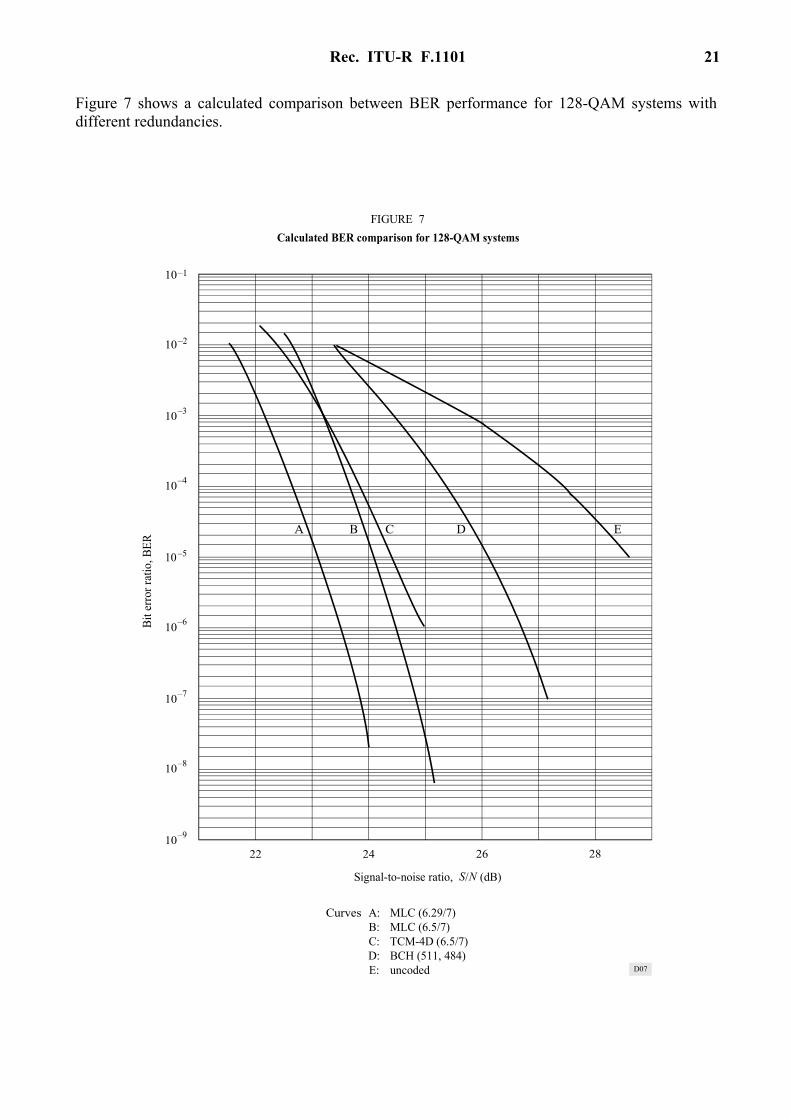
Figure 7 shows a calculated comparison between BER performance for 128-QAM systems with different redundancies.
A B C D E
22 24 26 28
–1
–2
–3
–4
–5
–6
–7
–8
–910
10
10
10
10
10
10
10
10
D07
Bit e
rror r
atio
, BER
Signal-to-noise ratio, S/N (dB)
FIGURE 7Calculated BER comparison for 128-QAM systems
Curves A: B:C:D:E:
MLC (6.29/7)MLC (6.5/7)TCM-4D (6.5/7)BCH (511, 484)uncoded
22 Rec. ITU-R F.1101
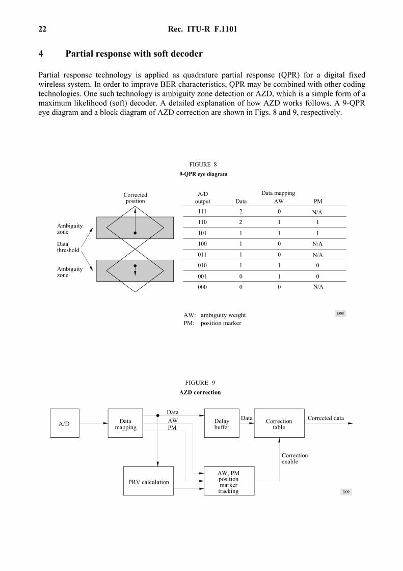
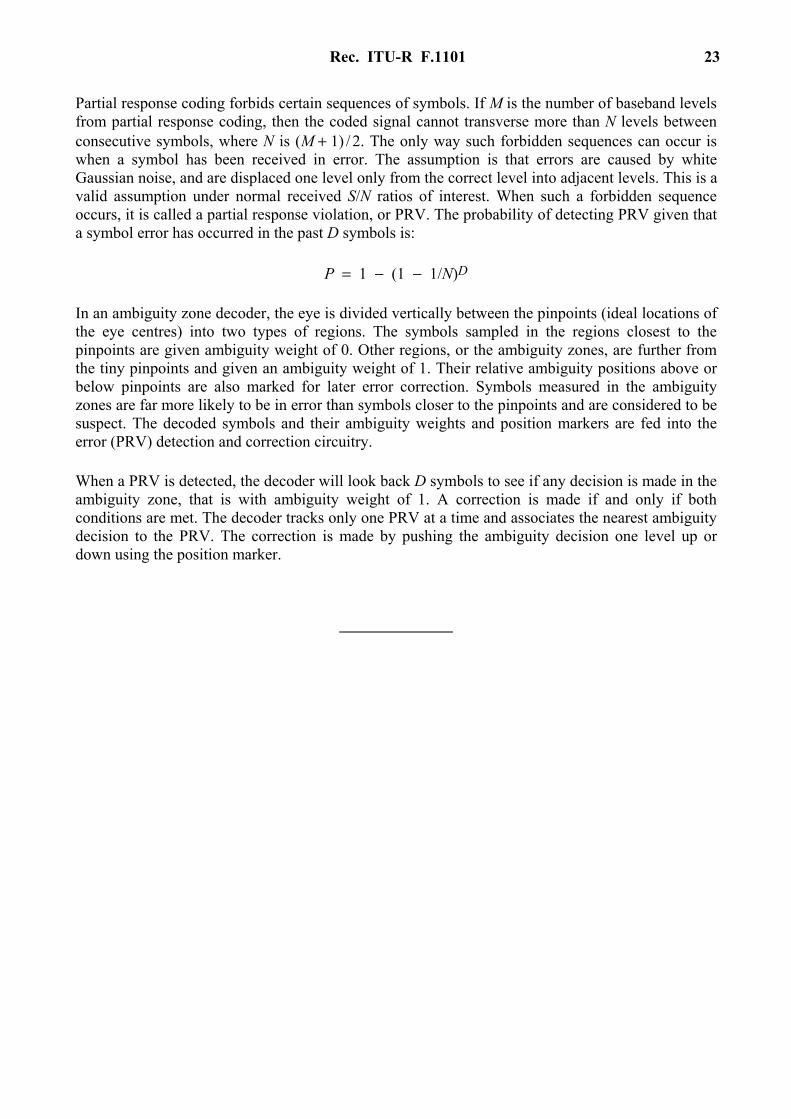
4 Partial response with soft decoder
Partial response technology is applied as quadrature partial response (QPR) for a digital fixed wireless system. In order to improve BER characteristics, QPR may be combined with other coding technologies. One such technology is ambiguity zone detection or AZD, which is a simple form of a maximum likelihood (soft) decoder. A detailed explanation of how AZD works follows. A 9-QPR eye diagram and a block diagram of AZD correction are shown in Figs. 8 and 9, respectively.
111
110
101
100
011
010
001
000
2
2
1
1
1
1
0
0
0
1
1
0
0
1
1
0
1
1
0
0
N/A
N/A
N/A
N/A
D08
Ambiguityzone
Datathreshold
Correctedposition
A/Doutput Data AW PM
Data mapping
FIGURE 89-QPR eye diagram
AW:PM:
ambiguity weightposition marker
Ambiguityzone
D09
FIGURE 9AZD correction
A/D Datamapping
Delaybuffer
AW, PMpositionmarkertracking
Correctiontable
DataData Corrected data
Correctionenable
AWPM
PRV calculation
Rec. ITU-R F.1101 23
Partial response coding forbids certain sequences of symbols. If M is the number of baseband levels from partial response coding, then the coded signal cannot transverse more than N levels between consecutive symbols, where N is (M + 1) / 2. The only way such forbidden sequences can occur is when a symbol has been received in error. The assumption is that errors are caused by white Gaussian noise, and are displaced one level only from the correct level into adjacent levels. This is a valid assumption under normal received S/N ratios of interest. When such a forbidden sequence occurs, it is called a partial response violation, or PRV. The probability of detecting PRV given that a symbol error has occurred in the past D symbols is:
P = 1 − (1 − 1/N)D
In an ambiguity zone decoder, the eye is divided vertically between the pinpoints (ideal locations of the eye centres) into two types of regions. The symbols sampled in the regions closest to the pinpoints are given ambiguity weight of 0. Other regions, or the ambiguity zones, are further from the tiny pinpoints and given an ambiguity weight of 1. Their relative ambiguity positions above or below pinpoints are also marked for later error correction. Symbols measured in the ambiguity zones are far more likely to be in error than symbols closer to the pinpoints and are considered to be suspect. The decoded symbols and their ambiguity weights and position markers are fed into the error (PRV) detection and correction circuitry.
When a PRV is detected, the decoder will look back D symbols to see if any decision is made in the ambiguity zone, that is with ambiguity weight of 1. A correction is made if and only if both conditions are met. The decoder tracks only one PRV at a time and associates the nearest ambiguity decision to the PRV. The correction is made by pushing the ambiguity decision one level up or down using the position marker.