Embed Size (px)
Citation preview
Rec. ITU-R BT.1683 1
RECOMMENDATION ITU-R BT.1683
Objective perceptual video quality measurement techniques for standard definition digital broadcast television in the presence of a full reference
(Question ITU-R 44/6)
(2004)
The ITU Radiocommunication Assembly,
considering
a) that the ability to measure automatically the quality of broadcast video has long been recognized as a valuable asset to the industry;
b) that conventional objective methods are no longer fully adequate for measuring the perceived video quality of digital video systems using compression;
c) that objective measurement of perceived video quality will complement conventional objective test methods;
d) that current formal subjective assessment methods are time-consuming and expensive and generally not suited for operational conditions;
e) that objective measurement of perceived video quality may usefully complement subjective assessment methods,
recommends
1 that the guidelines, scope and limitations given in Annex 1 be used in the application of the objective video quality models found in Annexes 2-5;
2 that the objective video quality models given in Annexes 2-5 be used for objective measurement of perceived video quality.
Annex 1
Summary
This Recommendation specifies methods for estimating the perceived video quality of a one-way video transmission system. This Recommendation applies to baseband signals. The estimation methods in this Recommendation are applicable to: – codec evaluation, specification, and acceptance testing; – potentially real-time, in-service quality monitoring at the source; – remote destination quality monitoring when a copy of the source is available; – quality measurement of a storage or transmission system that utilizes video compression
and decompression techniques, either a single pass or a concatenation of such techniques.
Introduction
The ability to measure automatically the quality of broadcast video has long been recognized as a valuable asset to the industry. The broadcast industry requires such tools to replace or supplement costly and time-consuming subjective quality testing. Traditionally, objective quality measurement has been obtained by calculating peak signal-to-noise ratios (PSNRs). Although a useful indicator
2 Rec. ITU-R BT.1683
of quality, PSNR has been shown to be a less than satisfactory representation of perceptual quality. To overcome the limitations associated with PSNR, research has been directed towards defining algorithms that can measure the perceptual quality of broadcast video. Such objective perceptual quality measurement tools may be applied to testing the performance of a broadcast network, as equipment procurement aids and in the development of new broadcast video coding techniques. In recent years, significant work has been dedicated to the development of reliable and accurate tools that can be used to objectively measure the perceptual quality of broadcast video. This Recommendation defines objective computational models that have been shown to be superior to PSNR as automatic measurement tools for assessing the quality of broadcast video. The models were tested on 525-line and 625-line material conforming to Recommendation ITU-R BT.601, which was characteristic of secondary distribution of digitally encoded television quality video.
The performance of the perceptual quality models was assessed through two parallel evaluations of the test video material1. In the first evaluation, a standard subjective method, the double stimulus continuous quality scale (DSCQS) method, was used to obtain subjective ratings of quality of video material by panels of human observers (Recommentdation ITU-R BT.500 – Methodology for the subjective assessment of the quality of television pictures). In the second evaluation, objective ratings were obtained by the objective computational models. For each model, several metrics were computed to measure the accuracy and consistency with which the objective ratings predicted the subjective ratings. Three independent laboratories conducted the subjective evaluation portion of the test. Two laboratories, Communications Research Center (CRC, Canada) and Verizon (United States of America), performed the test with 525/60 Hz sequences and a third lab, Fondazione Ugo Bordoni (FUB, Italy), performed the test with 625/50 Hz sequences. Several laboratories “proponents” produced objective computational models of the video quality of the same video sequences tested with human observers by CRC, Verizon and FUB. The results of the tests are given in Appendix 1.
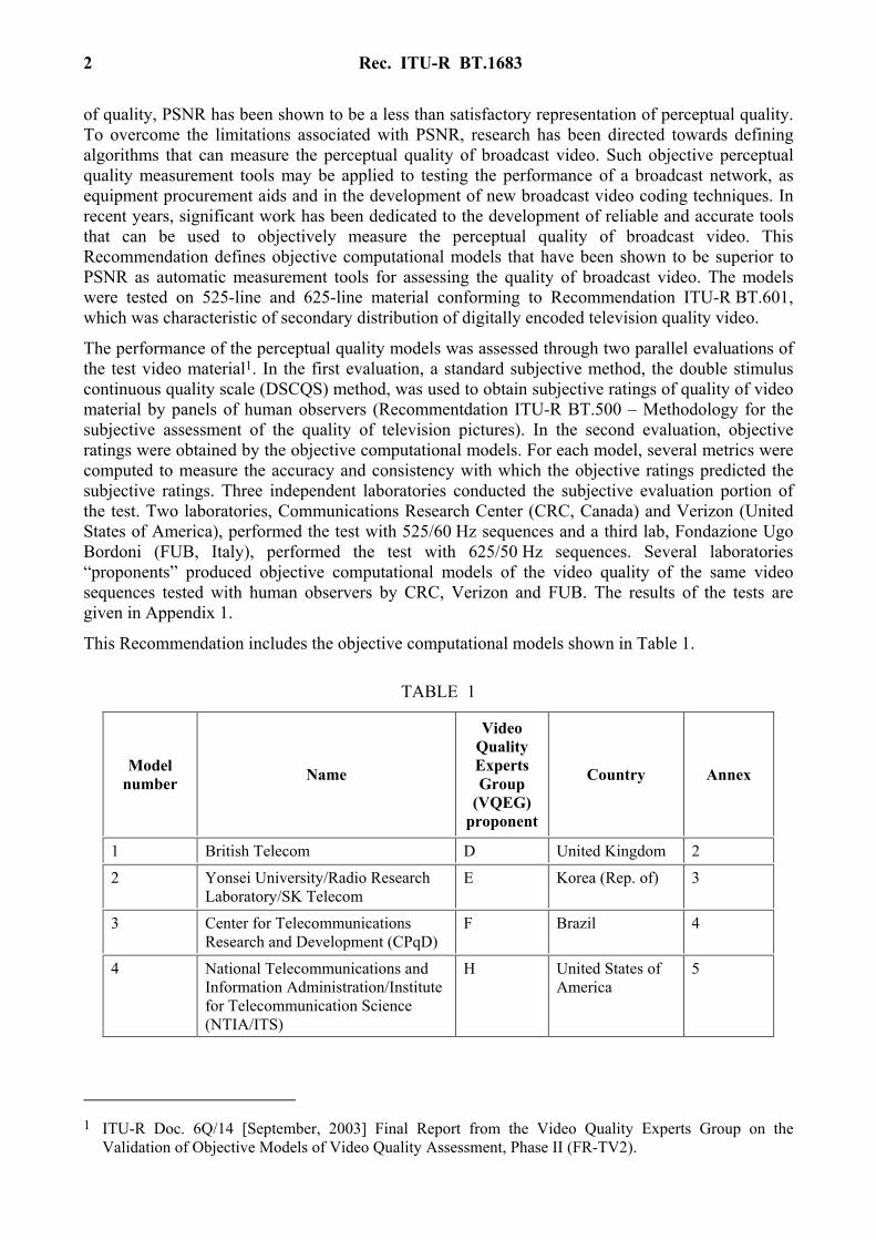
This Recommendation includes the objective computational models shown in Table 1.
TABLE 1
Model number Name
Video Quality Experts Group
(VQEG) proponent
Country Annex
1 British Telecom D United Kingdom 2
2 Yonsei University/Radio Research Laboratory/SK Telecom
E Korea (Rep. of) 3
3 Center for Telecommunications Research and Development (CPqD)
F Brazil 4
4 National Telecommunications and Information Administration/Institute for Telecommunication Science (NTIA/ITS)
H United States of America
5
1 ITU-R Doc. 6Q/14 [September, 2003] Final Report from the Video Quality Experts Group on the
Validation of Objective Models of Video Quality Assessment, Phase II (FR-TV2).
Rec. ITU-R BT.1683 3
A complete description of the above four objective computational models is provided in Annexes 2-5.
Existing video quality test equipment can be used until new test equipment implementing any of the four above models is readily available.
For any model to be considered for inclusion in the normative section of this Recommendation in the future, the model must be verified by an open independent body (such as VQEG) which will do the technical evaluation within the guidelines and performance criteria set out by Radiocommunication Study Group 6. The intention of Radiocommunication Study Group 6 is to eventually recommend only one normative full reference method.
1 Scope
This Recommendation specifies methods for estimating the perceived video quality of a one-way video system. This Recommendation applies to baseband signals. The objective video performance estimators are defined for the end-to-end quality between the two points. The estimation methods are based on processing 8-bit digital component video as defined by Recommendation ITU-R BT.6012. The encoder can utilize various compression methods (e.g. Moving Picture Experts Group (MPEG), ITU-T Recommendation H.263, etc.). The models proposed in this Recommendation may be used to evaluate a codec (encoder/decoder combination) or a concatenation of various compression methods and memory storage devices. While the derivation of the objective quality estimators described in this Recommendation might have considered error impairments (e.g. bit errors, dropped packets), independent testing results are not currently available to validate the use of the estimators for systems with error impairments. The validation test material did not contain channel errors.
1.1 Application
This Recommendation provides video quality estimations for television video classes (TV0-TV3), and multimedia video class (MM4) as defined in ITU-T Recommendation P.911, Annex B. The applications for the estimation models described in this Recommendation include but are not limited to: – codec evaluation, specification, and acceptance testing, consistent with the limited accuracy
as described below; – potentially real-time, in-service quality monitoring at the source; – remote destination quality monitoring when a copy of the source is available; – quality measurement of a storage or transmission system that utilizes video compression
and decompression techniques, either a single pass or a concatenation of such techniques.
1.2 Limitations
The estimation models described in this Recommendation cannot be used to replace subjective testing. Correlation values between two carefully designed and executed subjective tests (i.e. in two different laboratories) normally fall within the range 0.92 to 0.97. This Recommendation does not
2 This does not preclude implementation of the measurement method for one-way video systems that utilize
composite video input and outputs. Specification of the conversion between composite and component domains is not part of this Recommendation. For example, SMPTE 170M Standard specifies one method for performing this conversion for NTSC.
4 Rec. ITU-R BT.1683
supply a means for quantifying potential estimation errors. Users of this Recommendation should review the comparison of available subjective and objective results to gain an understanding of the range of video quality rating estimation errors.
The predicted performance of the estimation models is not currently validated for video systems with transmission channel error impairments.
Annex 2
Model 1
CONTENTS
Page
1 Introduction .................................................................................................................... 5
2 BTFR .............................................................................................................................. 5
3 Detectors......................................................................................................................... 5
3.1 Input conversion ................................................................................................. 6
3.2 Crop and offset ................................................................................................... 6
3.3 Matching ............................................................................................................. 7
3.3.1 Matching statistics................................................................................ 9
3.3.2 MPSNR ................................................................................................ 9
3.3.3 Matching Vectors ................................................................................. 9
3.4 Spatial frequency analysis .................................................................................. 10
3.4.1 Pyramid transform................................................................................ 10
3.4.2 Pyramid SNR ....................................................................................... 12
3.5 Texture analysis .................................................................................................. 12
3.6 Edge analysis ...................................................................................................... 13
3.6.1 Edge detection...................................................................................... 13
3.6.2 Edge differencing................................................................................. 13
3.7 MPSNR analysis................................................................................................. 14
4 Integration....................................................................................................................... 14
5 Registration..................................................................................................................... 15
6 References ...................................................................................................................... 15
Annex 2a .................................................................................................................................. 16

Rec. ITU-R BT.1683 5
1 Introduction
The BT full-reference (BTFR) automatic video quality assessment tool produces predictions of video quality that are representative of human quality judgements. This objective measurement tool digitally simulates features of the human visual system (HVS) to give accurate predictions of video quality and offers a viable alternative to costly and time-consuming formal subjective assessments.
A software implementation of the model was entered in the VQEG2 tests and the resulting performance presented in a test report.
2 BTFR
The BTFR algorithm consists of detection followed by integration as shown in Fig. 1. Detection involves the calculation of a set of perceptually meaningful detector parameters from the undistorted (reference) and distorted (degraded) video sequences. These parameters are then input to the integrator, which produces an estimate of the perceived video quality by appropriate weighting. The choice of detectors and weighting factors are founded on knowledge of the spatial and temporal masking properties of the HVS and determined through calibration experiments.
1683-01
Detectors Integration
Predicted videoquality
Reference video
Degraded video
TextureDegPySNR(3,3)EDiffXPerCentMPSNRSegVPSNR
FIGURE 1Full-reference video quality assessment model
MPSNR: matched PSNR
Input video of types 625 (720 × 576) interlaced at 50 fields/s and 525 (720 × 486) interlaced at 59.94 fields/s in YUV422 format are supported by the model.
3 Detectors
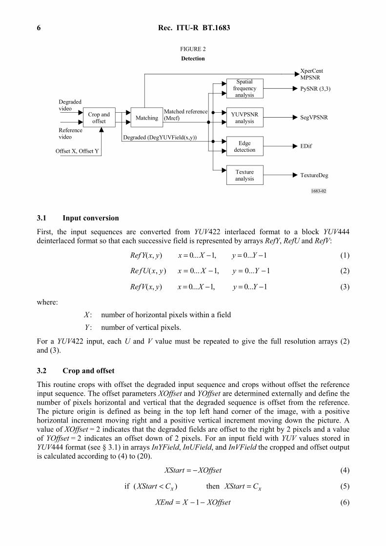
The detection module of the BTFR algorithm calculates a number spatial, temporal and frequency-based measures from the input YUV formatted sequences, as shown in Fig. 2.
6 Rec. ITU-R BT.1683
1683-02
Crop andoffset Matching
Matched reference(Mref)
Degraded (DegYUVField(x,y))
Degradedvideo
Referencevideo
Offset X, Offset Y
Spatialfrequencyanalysis
YUVPSNRanalysis
Edgedetection
Textureanalysis TextureDeg
EDif
SegVPSNR
PySNR (3,3)
XperCentMPSNR
FIGURE 2Detection
3.1 Input conversion
First, the input sequences are converted from YUV422 interlaced format to a block YUV444 deinterlaced format so that each successive field is represented by arrays RefY, RefU and RefV:
1...0,1...0),( −=−= YyXxyxYRef (1)
1...0,1...0),( −=−= YyXxyxUfRe (2)
1...0,1...0),( −=−= YyXxyxVRef (3)
where: X : number of horizontal pixels within a field Y : number of vertical pixels.
For a YUV422 input, each U and V value must be repeated to give the full resolution arrays (2) and (3).
3.2 Crop and offset
This routine crops with offset the degraded input sequence and crops without offset the reference input sequence. The offset parameters XOffset and YOffset are determined externally and define the number of pixels horizontal and vertical that the degraded sequence is offset from the reference. The picture origin is defined as being in the top left hand corner of the image, with a positive horizontal increment moving right and a positive vertical increment moving down the picture. A value of XOffset = 2 indicates that the degraded fields are offset to the right by 2 pixels and a value of YOffset = 2 indicates an offset down of 2 pixels. For an input field with YUV values stored in YUV444 format (see § 3.1) in arrays InYField, InUField, and InVField the cropped and offset output is calculated according to (4) to (20).
XOffsetXStart −= (4)
xx CXStartCXStart =< then)( if (5)
XOffsetXXEnd −−= 1 (6)

Rec. ITU-R BT.1683 7
1then)1( if −−=−−> xx CXXEndCXXEnd (7)
YOffsetYStart –= (8)
yy CYStartCYStart =< then)( if (9)
YOffsetYYEnd −−= 1 (10)
1then)1( if −−=−−> yy CYYEndCYYEnd (11)
X and Y give the horizontal and vertical field dimensions respectively and Cx and Cy the number of pixels to be cropped from left and right and top and bottom.
For 625 sequences,
10,30,288,720 ==== yx CCYX (12)
For 525 sequences,
10,30,243,720 ==== yx CCYX (13)
Xstart, Xend, Ystart and Yend now define the region of each field that will be copied. Pixels outside this region are initialized according to equations (14) to (15), where YField, UField and VField are XxY output pixel arrays containing Y, U and V values respectively.
The vertical bars to the left and right of the field are initialized according to:
1...01...1,1...00),( −=−+−== YyXXEndXStartxyxYField (14)
1...01...1,1...0128),(),( −=−+−=== YyXXEndXStartxyxVFieldyxUField (15)
The horizontal bars at the top and bottom of the field are initialized according to:
1...1,1...0,...0),( −+−=== YYEndYStartyXEndXStartxyxYField (16)
1...1,1...0...128),(),( −+−==== YYEndYStartyXEndXStartxyxVFieldyxUField (17)
Finally, the pixel values are copied according to:
YEndYStartyXEndXStartxYOffsetyXOffsetxInYFieldyxYField ......),(),( ==++= (18)
YEndYStartyXEndXStartxYOffsetyXOffsetxInUFieldyxUField ......),(),( ==++= (19)
YEndYStartyXEndXStartxYOffsetyXOffsetxInVFieldyxVField ......),(),( ==++= (20)
For the degraded input, cropping and shifting produces output field arrays DegYField, DegUField and DegVField, whilst cropping without shifting for the reference sequence produces RefYField, RefUField and RefVfield. These XxY two-dimensional arrays are used as inputs to detection routines described below.
3.3 Matching
The matching process produces signals for use within other detection procedures and also detection parameters for use in the integration procedure. The matching signals are generated from a process of finding the best match for small blocks within each degraded field from a buffer of neighbouring reference fields. This process yields a sequence, the matched reference, for use in place of the reference sequence in some of the detection modules.
8 Rec. ITU-R BT.1683
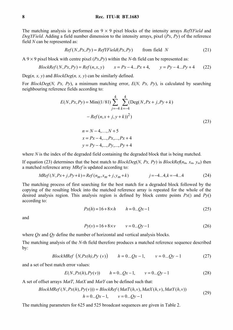
The matching analysis is performed on 9 × 9 pixel blocks of the intensity arrays RefYField and DegYField. Adding a field number dimension to the intensity arrays, pixel (Px, Py) of the reference field N can be represented as:
NPyPxRefYFieldPyPxNRef fieldfrom),(),,( = (21)
A 9 × 9 pixel block with centre pixel (Px,Py) within the N-th field can be represented as:
4...4,4...4),,(),,( +−=+−== PyPyyPxPxxyxnRefPyPxNBlockRef (22)
Deg(n, x, y) and BlockDeg(n, x, y) can be similarly defined.
For BlockDeg(N, Px, Py), a minimum matching error, E(N, Px, Py), is calculated by searching neighbouring reference fields according to:
4,...,,...,44,...,,...,4
5,,4
))),,(
),,(Deg()81/1((Min),,(
2
4
4
4
4
+−=+−=
+−=
++−
++= ∑∑−=−=
PyPyPyyPxPxPxx
NNn
kyjxnRef
kPyjPxNPyPxNEkj
K
(23)
where N is the index of the degraded field containing the degraded block that is being matched.
If equation (23) determines that the best match to BlockDeg(N, Px, Py) is BlockRef(nm, xm, ym) then a matched reference array MRef is updated according to:
4...4,4...4),,(),,( −=−=++=++ kjkyjxnRefkPyjPxNMRef mmm (24)
The matching process of first searching for the best match for a degraded block followed by the copying of the resulting block into the matched reference array is repeated for the whole of the desired analysis region. This analysis region is defined by block centre points Px() and Py() according to:
1...0816)( −=×+= QxhhhPx (25)
and
1...0816)( −=×+= QyvvvPy (26)
where Qx and Qy define the number of horizontal and vertical analysis blocks.
The matching analysis of the N-th field therefore produces a matched reference sequence described by:
( ) 1...0,1...0)( −=−= QyvQxhvN,Px(h),PyBlockMRef (27)
and a set of best match error values:
1...0,1...0))(),(,( −=−= QyvQxhvPyhPxNE (28)
A set of offset arrays MatT, MatX and MatY can be defined such that:
1...0,1...0
)),(),,(),,(()))(),(,(−=−=
=QyvQxh
vhMatYvhMatXvhMatTBlockRefvPyhPxNBlockMRef (29)
The matching parameters for 625 and 525 broadcast sequences are given in Table 2.

Rec. ITU-R BT.1683 9
TABLE 2
Search parameters for matching procedure
The analysis region defined by equations (26) and (27) does not cover the complete field size. MRef must therefore be initialized according to equation (29) so that it may be used elsewhere unrestricted.
1...0,1...00),( −=−== YyXxyxMRef (30)
3.3.1 Matching statistics
Horizontal matching statistics from the matching process are calculated for use in the integration process. The best match for each analysis block, determined according to equation (23), is used in the construction of the histogram histX for each field according to:
1...0,1...0
1)4)(),((4)(),((−=−=
++−=+−QxvQxh
hPxvhMatXhistXhPxvhMatXhistX (31)
where array histX is initialized to zero for each field. The histogram is then used to determine the measure fXPerCent according to:
8...0)(/))((Max1008
0=×= ∑
=ijhistXihistXXPerCentf
j (32)
For each field, the fXPerCent measure gives the proportion (%) of matched blocks that contribute to the peak of the matching histogram.
3.3.2 MPSNR
The minimum error, E(), for each matched block is used to calculate a matched SNR according to:
××=
>
∑ ∑
∑∑−
=
−
=
−
=
−
=
1
0
1
0
210
1
0
1
0
))(),(,(255log10
then0))(),(,(if
/Qx
h
Qy
v
Qy
v
Qx
h
vPyhPxNEQyQxMPSNR
vPyhPxNE
(33)
)255(log10then0))(),(,(if 210
1
0
1
0==
∑∑
−
=
−
=MPSNRvPyhPxNE
Qy
v
Qx
h (34)
3.3.3 Matching vectors
Horizontal, vertical and delay vectors are stored for later use according to:
1...0,1...0),(),( −=−=−= QyvQxhNvhMatTvhSyncT (35)
1...0,1...0)(),(),( −=−=−= QyvQxhhPxvhMatXvhSyncX (36)
Parameter 625 525 Qx 87 87 Qy 33 28
10 Rec. ITU-R BT.1683
1...0,1...0)(),(),( −=−=−= QyvQxhhPyvhMatYvhSyncY (37)
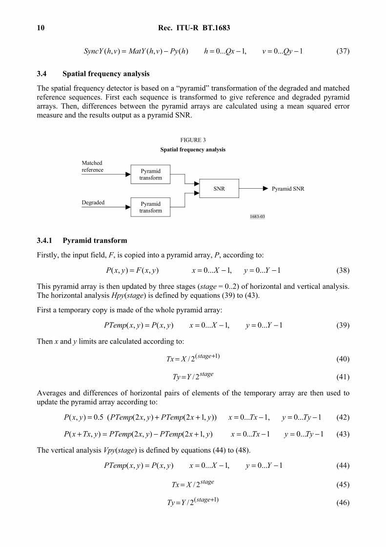
3.4 Spatial frequency analysis
The spatial frequency detector is based on a “pyramid” transformation of the degraded and matched reference sequences. First each sequence is transformed to give reference and degraded pyramid arrays. Then, differences between the pyramid arrays are calculated using a mean squared error measure and the results output as a pyramid SNR.
1683-03
Pyramidtransform
Pyramidtransform
SNR Pyramid SNR
Matchedreference
Degraded
FIGURE 3Spatial frequency analysis
3.4.1 Pyramid transform
Firstly, the input field, F, is copied into a pyramid array, P, according to:
1...0,1...0),(),( −=−== YyXxyxFyxP (38)
This pyramid array is then updated by three stages (stage = 0..2) of horizontal and vertical analysis. The horizontal analysis Hpy(stage) is defined by equations (39) to (43).
First a temporary copy is made of the whole pyramid array:
1...0,1...0),(),( −=−== YyXxyxPyxPTemp (39)
Then x and y limits are calculated according to:
)1(2/ += stageXTx (40)
stageYTy 2/= (41)
Averages and differences of horizontal pairs of elements of the temporary array are then used to update the pyramid array according to:
1...0,1...0)),12(),2((5.0),( −=−=++= TyyTxxyxPTempyxPTempyxP (42)
1...01...0),12(),2(),( −=−=+−=+ TyyTxxyxPTempyxPTempyTxxP (43)
The vertical analysis Vpy(stage) is defined by equations (44) to (48).
1...0,1...0),(),( −=−== YyXxyxPyxPTemp (44)
stageXTx 2/= (45)
)1(2/ += stageYTy (46)

Rec. ITU-R BT.1683 11
Averages and differences of vertical pairs of elements of the temporary array are then used to update the pyramid array according to:
1...0,1...0))12,()2,((5.0),( −=−=++= TyyTxxyxPTempyxPTempyxP (47)
1...01...0)12,()2,(),( −=−=+−=+ TyyTxxyxPTempyxPTempTyyxP (48)
For stage 0, the horizontal analysis Hpy(0) followed by the vertical analysis Vpy(0) updates the whole of the pyramid array with the 4 quadrants Q(stage, 0...3) constructed according to:
1683-04
Q(0,0) Q(0,1)
Q(0,2) Q(0,3)
FIGURE 4Quadrant output from stage 0 analysis
Q(0,0) = average of blocks of 4Q(0,1) = horizontal difference of blocks of 4Q(0,2) = vertical difference of blocks of 4Q(0,3) = diagonal difference of blocks of 4
Stage 1 analysis is then performed on Q(0,0) to give results Q(1,0...3) that are stored in the pyramid according to:
1683-05
Q(1,0)Q(0,1)
Q(0,2) Q(0,3)
Q(1,1)
Q(1,2) Q(1,3)
FIGURE 5Quadrant output from stage 1 analysis
Stage 2 analysis processes Q(1,0) and overwrites it with Q(2,0...3).
After the three stages of analysis, the resulting pyramid array has a total of 10 blocks of results. Three blocks Q(0,1...3) are from the stage 0,2 × 2 pixel analysis, three Q(1,1...3) from the stage 1, 4 × 4 analysis and 4 Q(2,0...3) from the stage 2, 8 × 8 analysis.
The three-stage analysis of the matched reference and degraded sequences produce the pyramid arrays Pref and Pdeg. Differences between these arrays are then measured in the pyramid SNR module.

12 Rec. ITU-R BT.1683
3.4.2 Pyramid SNR
A squared error measure between the reference and degraded pyramid arrays is determined over quadrants 1 to 3 of stages 0 to 2 according to:
3...12...0)),(),(()/1(),(1),(2
),(1
1),(2
),(1
22 ==−= ∑ ∑−
=
−
=qsyxPdegyxPrefXYqsE
qsx
qsxx
qsy
qsyy (49)
where x1, x2, y1 and y2 define the horizontal and vertical limits of the quadrants within the pyramid arrays and are calculated according to:
)1()1( 2/)1,(20)1,(1)1,(12)1,(22/)1,(1 ++ ==×== ss YsysysxsxXsx (50)
)2,(12)2,(22/)2,(12/)2,(20)2,(1 )1()1( sysyYsyXsxsx ss ×==== ++ (51)
)3,(12)3,(22/)3,(1)3,(12)3,(22/)3,(1 )1()1( sysyYsysxsxXsx ss ×==×== ++ (52)
The results from equation (49) are then used to determine a PSNR measure for each quadrant of each field according to:
)255(log10 then
)),(/255(log10),()0,0(if22
10
210
XYSNR
qsEqsPySNRE
×=
=> (53)
where the number of stages s = 0...2 and the number of quadrants for each stage q = 1...3.
3.5 Texture analysis
The texture of the degraded sequence is measured by recording the number of turning-points in the intensity signal along horizontal picture lines. This may be calculated according to equations (54) to (59).
For each field, first a turning-point counter is initialized according to equation (54).
sum = 0 (54)
Then, each line, y = 0...Y − 1, is processed for x = 0...X − 2 according:
0_,0_ == neglastposlast (55)
),1(),()( yxPyxPxdif +−= (56)
1))__()0)((( if +=<< sumsumposlastneglastANDxdif (57)
1))__()0)((( if +=>> sumsumposlastneglastANDxdif (58)
xposlastxdif => _)0)(( if (59)
xneglastxdif =< _)0)(( if (60)
When all the lines for a field have been processed, the counter, sum, will contain the number of turning-points in the horizontal intensity signal. This is then used to calculate a texture parameter for each field according to:
XYsumTextureDeg /100×= (61)

Rec. ITU-R BT.1683 13
3.6 Edge analysis
Each field of the degraded and matched reference sequences is separately passed through an edge detection routine to produce corresponding edge field maps, which are then compared in a block matching procedure to produce the detection parameters.
1683-06
Edgedetection
Edgedetection
Blockmatching EDif parameters
Matchedreference
Degraded
FIGURE 6Edge analysis
EMapRef
EMapDeg
3.6.1 Edge detection
A Canny edge detector [Canny, 1986] was used to determine the edge maps, but other similar edge detection techniques may be used. The resulting edge maps, EMapRef and EMapDeg, are pixel maps with an edge indicated by a 1 and no edge by 0.
For an edge detected at pixel (x, y):
1...0,1...01),( −=−== YyXxyxEMap (62)
For no edge detected at pixel (x, y):
1...0,1...00),( −=−== YyXxyxEMap (63)
3.6.2 Edge differencing
The edge differencing procedure measures the differences between the edge maps for corresponding degraded and matched reference fields. The analysis is performed in NxM pixel non-overlapping blocks according to equations (64) to (68).
First, a measure of the number of edge-marked pixels in each analysis block is calculated, where Bh and Bv define the number of non-overlapping blocks to be analysed in the horizontal and vertical directions and X1 and Y1 define analysis offsets from the field edge.
1...0,1...0)1,1(),(2
1
2
1−=−=++++= ∑∑
==BvyBhxjYMyiXNxEMapRefyxBref
j
jj
i
ii (64)
∑∑==
−=−=++++=2
1
2
11...0,1...0)1,1(),(
j
jj
i
iiBvyBhxjYMyiXNxEMapDegyxBDeg (65)
The summation limits are determined according to:
2div)1(2)2div(1 −=−= NiNi (66)
2div)1(2)2div(1 −=−= MjMj (67)
where the “div” operator represents an integer division.

14 Rec. ITU-R BT.1683
Then, a measure of the differences over the whole field is calculated according to:
Bv
y
Bh
xyxBDegyxfReBBvBhMNEDif
/11
0
1
0)),(),(()(/1 )(
−= ∑∑
−
=
−
= (68)
For 720 × 288 pixel fields for 625 broadcast video:
3,69,101,4178,61,4 ======= QBvYMBhXN (69)
For 720 × 243 pixel fields for 525 broadcast video:
3,58,101,4178,61,4 ======= QBvYMBhXN (70)
3.7 MPSNR analysis
A matched signal to noise ratio is calculated for the pixel V values by use of the matching vectors defined in equations (35) to (37). For each set of matching vectors, an error measure, VE, is calculated according to:
2
4
4
4
4
))),()(,),()(),,((
))(,)(,(()81/1(),(
jvhSyncYvPyivhSyncXhPxvhSyncTNRefVField
jhPyihPxNDegVvhVEi j
+++++
−++= ∑ ∑−= −= (71)
A segmental PSNR measure is then calculated for the field according to:
)( )1),((/255log10)/1( 210
1
0
1
0+= ∑∑
−
=
−
=vhVEQyQxSegVPSNR
Qy
v
Qx
h (72)
4 Integration
The integration procedure firstly requires the time averaging of the field-by-field detection parameters according to equation (73):
5...0),()/1()(1
0== ∑
−
=knkDNkAvD
N
n (73)
where:
N : total number of fields in the tested sequences
D(k, n) : detection parameter k for field n.
The averaged detection parameters, AvD(k), are then combined to give a predicted quality score, PDMOS, for the N field sequence according to equation (74):
∑=
×+=5
0)()(
kkWkAvDOffsetPDMOS (74)
Tables 3 and 4 show the integrator parameters for 625 and 525 sequences respectively.

Rec. ITU-R BT.1683 15
TABLE 3
Integration parameters for 625 broadcast video
TABLE 4
Integration parameters for 525 broadcast video
5 Registration
The FR model requires both spatial and temporal alignment to operate effectively. The model incorporates inherent alignment and can accommodate spatial offsets between the reference and degraded sequences ±4 pixels and temporal offset of ±4 fields. Spatial and temporal offsets beyond these limits are not handled by the model and a separate registration module will be required to ensure the reference and degraded files are properly aligned.
6 References
CANNY. J. [1986] A computational approach to edge detection. IEEE Trans. Pattern Analysis and Machine Intelligence. Vol. 8(6), p. 679-698.
K Parameter name W
0 TextureDeg –0.68 1 PySNR(3,3) –0.57 2 EDif +58 913.294 3 fXPerCent –0.208 4 MPSNR –0.928 5 SegVPSNR –1.529 Offset +176.486 N 400
K Parameter name W
0 TextureDeg +0.043 1 PySNR(3,3) –2.118 2 EDif +60 865.164 3 fXPerCent –0.361 4 MPSNR +1.104 5 SegVPSNR –1.264 Offset +260.773 N 480

16 Rec. ITU-R BT.1683
Annex 2a
TABLE 5
525 subjective and objective data
Filename Source sequence
(SRC)
Hypothetical reference circuit
(HRC)
Raw mean subjective
rating
Model predicted
rating based on raw data
Scaled mean subjective
rating
Model predicted
rating based on scaled data
V2src01_hrc01_525.yuv 1 1 –38.30757576 44.945049 0.5402368 0.69526
V2src01_hrc02_525.yuv 1 2 –39.56212121 38.646271 0.5483205 0.58989
V2src01_hrc03_525.yuv 1 3 –25.9469697 32.855755 0.4024097 0.50419
V2src01_hrc04_525.yuv 1 4 –17.24090909 21.062775 0.3063528 0.36089
V2src02_hrc01_525.yuv 2 1 –35.23636364 31.260744 0.5025558 0.48242
V2src02_hrc02_525.yuv 2 2 –18.01818182 18.732758 0.3113346 0.33715
V2src02_hrc03_525.yuv 2 3 –6.284848485 8.914509 0.1881739 0.25161
V2src02_hrc04_525.yuv 2 4 –6.983333333 4.16663 0.1907347 0.21776
V2src03_hrc01_525.yuv 3 1 –31.96515152 22.348713 0.4682724 0.37461
V2src03_hrc02_525.yuv 3 2 –17.47727273 10.44728 0.3088831 0.26352
V2src03_hrc03_525.yuv 3 3 –1.104545455 2.494911 0.1300389 0.20688
V2src03_hrc04_525.yuv 3 4 –1.171212121 0 0.1293293 0.19158
V2src04_hrc05_525.yuv 4 5 –50.64090909 40.82526 0.6742005 0.6249
V2src04_hrc06_525.yuv 4 6 –28.05454545 32.552322 0.4250873 0.49999
V2src04_hrc07_525.yuv 4 7 –23.87575758 25.286598 0.3762656 0.40764
V2src04_hrc08_525.yuv 4 8 –16.60757576 19.86405 0.2972294 0.3485
V2src05_hrc05_525.yuv 5 5 –31.86969697 30.812616 0.4682559 0.47645
V2src05_hrc06_525.yuv 5 6 –18.56515152 21.413895 0.3203024 0.3646
V2src05_hrc07_525.yuv 5 7 –8.154545455 15.446437 0.2071702 0.306
V2src05_hrc08_525.yuv 5 8 –4.006060606 10.836051 0.1652752 0.26662
V2src06_hrc05_525.yuv 6 5 –41.63181818 37.342789 0.5690291 0.56967
V2src06_hrc06_525.yuv 6 6 –29.48787879 26.660055 0.4370961 0.42391
V2src06_hrc07_525.yuv 6 7 –22.25909091 20.878248 0.3591788 0.35896
V2src06_hrc08_525.yuv 6 8 –12.03181818 16.896168 0.2482169 0.31941
V2src07_hrc05_525.yuv 7 5 –23.89545455 19.086998 0.3796362 0.34067
V2src07_hrc06_525.yuv 7 6 –10.15606061 10.69402 0.2276934 0.26548
V2src07_hrc07_525.yuv 7 7 –4.240909091 4.896546 0.1644409 0.22267
V2src07_hrc08_525.yuv 7 8 –5.98030303 1.555055 0.1819566 0.20099
V2src08_hrc09_525.yuv 8 9 –76.2 52.094177 0.9513387 0.83024
V2src08_hrc10_525.yuv 8 10 –61.34545455 47.395226 0.789748 0.7397
V2src08_hrc11_525.yuv 8 11 –66.02575758 52.457584 0.8405916 0.83753

Rec. ITU-R BT.1683 17
TABLE 5
525 subjective and objective data
Filename Source sequence
(SRC)
Hypothetical reference circuit
(HRC)
Raw mean subjective
rating
Model predicted
rating based on raw data
Scaled mean subjective
rating
Model predicted
rating based on scaled data
V2src08_hrc12_525.yuv 8 12 –37.20454545 37.931854 0.5221555 0.57874
V2src08_hrc13_525.yuv 8 13 –31.23030303 30.95985 0.4572049 0.4784
V2src08_hrc14_525.yuv 8 14 –31.26818182 33.293602 0.4614104 0.51031
V2src09_hrc09_525.yuv 9 9 –64.42878788 54.414772 0.8262912 0.87746
V2src09_hrc10_525.yuv 9 10 –49.92878788 36.080425 0.660339 0.55061
V2src09_hrc11_525.yuv 9 11 –53.73181818 46.338791 0.7100111 0.72031
V2src09_hrc12_525.yuv 9 12 –34.36969697 23.21393 0.4921708 0.38409
V2src09_hrc13_525.yuv 9 13 –22.85454545 16.955978 0.3656559 0.31998
V2src09_hrc14_525.yuv 9 14 –16.41666667 13.694396 0.2960957 0.29046
V2src10_hrc09_525.yuv 10 9 –72.11212121 48.179104 0.9084171 0.75433
V2src10_hrc10_525.yuv 10 10 –43.11666667 30.703861 0.5908784 0.475
V2src10_hrc11_525.yuv 10 11 –56.11969697 52.63887 0.7302376 0.84118
V2src10_hrc12_525.yuv 10 12 –19.55909091 21.95225 0.3345703 0.37033
V2src10_hrc13_525.yuv 10 13 –12.34393939 16.23988 0.2565459 0.31328
V2src10_hrc14_525.yuv 10 14 –16.05 23.201355 0.2953144 0.38395
V2src11_hrc09_525.yuv 11 9 –50.40454545 36.394535 0.6675853 0.55531
V2src11_hrc10_525.yuv 11 10 –54.26212121 37.812542 0.7054929 0.5769
V2src11_hrc11_525.yuv 11 11 –41.73636364 44.128036 0.5761193 0.68087
V2src11_hrc12_525.yuv 11 12 –19.03939394 14.619688 0.32761 0.29857
V2src11_hrc13_525.yuv 11 13 –17.72121212 14.12041 0.310495 0.29417
V2src11_hrc14_525.yuv 11 14 –19.4969697 14.927424 0.331051 0.30132
V2src12_hrc09_525.yuv 12 9 –61.35 40.051254 0.7883371 0.61229
V2src12_hrc10_525.yuv 12 10 –46.84545455 31.128973 0.6295301 0.48066
V2src12_hrc11_525.yuv 12 11 –51.80151515 41.77285 0.6809288 0.6406
V2src12_hrc12_525.yuv 12 12 –22.51969697 20.868282 0.3651402 0.35886
V2src12_hrc13_525.yuv 12 13 –14.17878788 15.040992 0.2714356 0.30234
V2src12_hrc14_525.yuv 12 14 –14.6030303 13.521517 0.2782449 0.28896
V2src13_hrc09_525.yuv 13 9 –55.25 38.691498 0.7211194 0.5906
V2src13_hrc10_525.yuv 13 10 –39.55 33.054504 0.5545722 0.50696
V2src13_hrc11_525.yuv 13 11 –40.03939394 45.9454 0.5525494 0.71318
V2src13_hrc12_525.yuv 13 12 –14 16.631002 0.2708744 0.31692
V2src13_hrc13_525.yuv 13 13 –14.33181818 15.113959 0.27549 0.30299
V2src13_hrc14_525.yuv 13 14 –14.31969697 16.611286 0.2733771 0.31674

18 Rec. ITU-R BT.1683
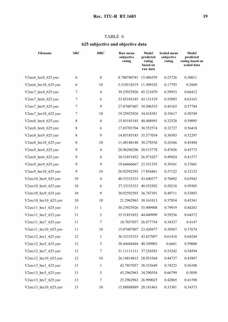
TABLE 6
625 subjective and objective data
Filename SRC HRC Raw mean subjective
rating
Model predicted
rating based on raw data
Scaled mean subjective
rating
Model predicted
rating based on scaled data
V2src1_hrc2_625.yuv 1 2 38.85185185 31.764214 0.59461 0.47326
V2src1_hrc3_625.yuv 1 3 42.07407407 21.868561 0.64436 0.36062
V2src1_hrc4_625.yuv 1 4 23.77777778 12.195552 0.40804 0.27239
V2src1_hrc6_625.yuv 1 6 18.14814815 9.169512 0.34109 0.24887
V2src1_hrc8_625.yuv 1 8 12.92592593 6.738072 0.2677 0.23128
V2src1_hrc10_625.yuv 1 10 11.88888889 2.553883 0.26878 0.20356
V2src2_hrc2_625.yuv 2 2 33.51851852 31.492788 0.54173 0.46985
V2src2_hrc3_625.yuv 2 3 46.48148148 31.1313 0.70995 0.46535
V2src2_hrc4_625.yuv 2 4 13.33333333 20.241726 0.27443 0.34432
V2src2_hrc6_625.yuv 2 6 8.814814815 17.39045 0.22715 0.31721
V2src2_hrc8_625.yuv 2 8 7.074074074 14.914576 0.21133 0.29513
V2src2_hrc10_625.yuv 2 10 3.407407407 7.352309 0.16647 0.23562
V2src3_hrc2_625.yuv 3 2 48.07407407 38.852715 0.73314 0.56845
V2src3_hrc3_625.yuv 3 3 50.66666667 38.244621 0.76167 0.55982
V2src3_hrc4_625.yuv 3 4 32.11111111 27.733229 0.49848 0.42454
V2src3_hrc6_625.yuv 3 6 22.33333333 24.80323 0.38613 0.39159
V2src3_hrc8_625.yuv 3 8 16.33333333 23.296747 0.34574 0.37544
V2src3_hrc10_625.yuv 3 10 11.96296296 16.33028 0.26701 0.30759
V2src4_hrc2_625.yuv 4 2 36.14814815 42.041592 0.58528 0.61514
V2src4_hrc3_625.yuv 4 3 55.03703704 49.283836 0.90446 0.72942
V2src4_hrc4_625.yuv 4 4 39.7037037 38.322186 0.62361 0.56091
V2src4_hrc6_625.yuv 4 6 38.03703704 36.863457 0.61143 0.54053
V2src4_hrc8_625.yuv 4 8 24.40740741 32.46579 0.43329 0.48214
V2src4_hrc10_625.yuv 4 10 12.88888889 25.918123 0.26548 0.40388
V2src5_hrc2_625.yuv 5 2 38.62962963 38.95779 0.61973 0.56995
V2src5_hrc3_625.yuv 5 3 44.18518519 40.076313 0.68987 0.58609
V2src5_hrc4_625.yuv 5 4 24.66666667 23.166002 0.41648 0.37406
V2src5_hrc6_625.yuv 5 6 23.62962963 20.592213 0.4218 0.34778
V2src5_hrc8_625.yuv 5 8 12.40740741 13.763152 0.27543 0.28531
V2src5_hrc10_625.yuv 5 10 7.37037037 8.418313 0.2022 0.24332
V2src6_hrc2_625.yuv 6 2 22.48148148 33.810165 0.38852 0.49949
V2src6_hrc3_625.yuv 6 3 27.07407407 25.004984 0.44457 0.39379
V2src6_hrc4_625.yuv 6 4 13.18518519 20.889347 0.27983 0.35074
V2src6_hrc6_625.yuv 6 6 14.44444444 17.418222 0.28106 0.31747
Rec. ITU-R BT.1683 19
TABLE 6
625 subjective and objective data
Filename SRC HRC Raw mean subjective
rating
Model predicted
rating based on raw data
Scaled mean subjective
rating
Model predicted
rating based on scaled data
V2src6_hrc8_625.yuv 6 8 8.740740741 15.486559 0.23726 0.30011
V2src6_hrc10_625.yuv 6 10 5.518518519 11.509192 0.17793 0.2669
V2src7_hrc4_625.yuv 7 4 39.25925926 45.231079 0.59953 0.66412
V2src7_hrc6_625.yuv 7 6 33.85185185 43.131519 0.55093 0.63163
V2src7_hrc9_625.yuv 7 9 27.07407407 39.506535 0.45163 0.57784
V2src7_hrc10_625.yuv 7 10 19.25925926 34.418381 0.35617 0.50749
V2src8_hrc4_625.yuv 8 4 15.85185185 40.408993 0.32528 0.59095
V2src8_hrc6_625.yuv 8 6 17.03703704 38.552574 0.32727 0.56418
V2src8_hrc9_625.yuv 8 9 14.85185185 35.577034 0.30303 0.52297
V2src8_hrc10_625.yuv 8 10 11.48148148 30.278536 0.26366 0.45484
V2src9_hrc4_625.yuv 9 4 28.96296296 30.515778 0.47656 0.45775
V2src9_hrc6_625.yuv 9 6 30.51851852 26.971027 0.49924 0.41577
V2src9_hrc9_625.yuv 9 9 19.66666667 23.351355 0.39101 0.37601
V2src9_hrc10_625.yuv 9 10 20.92592593 17.856861 0.37122 0.32152
V2src10_hrc4_625.yuv 10 4 40.33333333 43.640377 0.70492 0.63942
V2src10_hrc6_625.yuv 10 6 37.33333333 40.552502 0.58218 0.59305
V2src10_hrc9_625.yuv 10 9 30.92592593 36.747391 0.49711 0.53893
V2src10_hrc10_625.yuv 10 10 21.2962963 30.161013 0.37854 0.45341
V2src11_hrc1_625.yuv 11 1 50.25925926 55.909908 0.79919 0.84263
V2src11_hrc5_625.yuv 11 5 35.51851852 44.049999 0.59256 0.64572
V2src11_hrc7_625.yuv 11 7 18.7037037 26.877754 0.34337 0.4147
V2src11_hrc10_625.yuv 11 10 15.07407407 23.420477 0.30567 0.37674
V2src12_hrc1_625.yuv 12 1 36.33333333 43.837097 0.61418 0.64244
V2src12_hrc5_625.yuv 12 5 38.44444444 40.349903 0.6661 0.59008
V2src12_hrc7_625.yuv 12 7 31.11111111 37.254383 0.53242 0.54594
V2src12_hrc10_625.yuv 12 10 26.14814815 28.953564 0.44737 0.43887
V2src13_hrc1_625.yuv 13 1 43.7037037 38.333649 0.74225 0.56108
V2src13_hrc5_625.yuv 13 5 43.2962963 34.290554 0.66799 0.5058
V2src13_hrc7_625.yuv 13 7 25.2962963 26.990025 0.42065 0.41598
V2src13_hrc10_625.yuv 13 10 15.88888889 20.181463 0.33381 0.34373
20 Rec. ITU-R BT.1683
Annex 3
Model 2
CONTENTS
Page
1 Introduction .................................................................................................................... 20
2 Objective measurement of video quality based on edge degradation ............................ 21
2.1 Edge PSNR (EPSNR) ......................................................................................... 21
2.2 Post adjustments ................................................................................................. 28
2.2.1 De-emphasis of high EPSNR............................................................... 28
2.2.2 Considering blurred edges ................................................................... 28
2.2.3 Scaling.................................................................................................. 29
2.3 Registration accuracy.......................................................................................... 29
2.4 The block diagram of the model ......................................................................... 29
3 Objective data ................................................................................................................. 29
4 Conclusion...................................................................................................................... 29
5 References ...................................................................................................................... 29
1 Introduction
Traditionally, the evaluation of video quality is performed by a number of evaluators who subjectively evaluate the video quality. The evaluation can be done with or without reference videos. In referenced evaluation, evaluators are shown two videos: the reference (source) video and the processed video that is to be compared with the source video. By comparing the two videos, the evaluators give subjective scores to the videos. Therefore, it is often called a subjective test of video quality. Although the subjective test is considered to be the most accurate method since it reflects human perception, it has several limitations. First of all, it requires a number of evaluators. Thus, it is time-consuming and expensive. Furthermore, it cannot be done in real time. As a result, there has been a great interest in developing objective methods for video quality measurement. An important requirement for an objective method for video quality measurement is that it should provide consistent performance results over a wide range of video sequences that are not used in the design stage. Toward this goal, a model was developed, which is easy to implement, fast enough for real-time implementations and robust over a wide range of video impairments. The model is a product of collaborative works from Yonsei University, SK Telecom, and Radio Research Laboratory, Republic of Korea.

Rec. ITU-R BT.1683 21
2 Objective measurement of video quality based on edge degradation
2.1 Edge PSNR (EPSNR)
The model for objective video quality measurement is a full reference method. In other words, it is assumed that a reference video is provided. By analysing how humans perceive video quality, it is observed that the human visual system is sensitive to degradation around the edges. In other words, when the edge areas of a video are blurred, evaluators tend to give low scores to the video even though the overall mean squared error is small. It is further observed that video compression algorithms tend to produce more artefacts around edge areas. Based on this observation, the model provides an objective video quality measurement method that measures degradation around the edges. In the model, an edge detection algorithm is first applied to the source video sequence to locate the edge areas. Then, the degradation of those edge areas is measured by computing the mean squared error. From this mean squared error, the EPSNR is computed and used as a video quality metric after post-processing.
In the model, an edge detection algorithm needs to be first applied to locate edge areas. One can use any edge detection algorithm, though there may be minor differences in the results. For example, one can use any gradient operator to locate edge areas. A number of gradient operators have been proposed. In many edge detection algorithms, the horizontal gradient image ghorizontal(m,n) and the vertical gradient image gvertical(m,n) are first computed using gradient operators. Then, the magnitude gradient image g(m, n) may be computed as follows:
),(),(),( nmgnmgnmg verticalhorizontal +=
Finally, a thresholding operation is applied to the magnitude gradient image g(m, n) to find edge areas. In other words, pixels whose magnitude gradients exceed a threshold value are considered as edge areas.
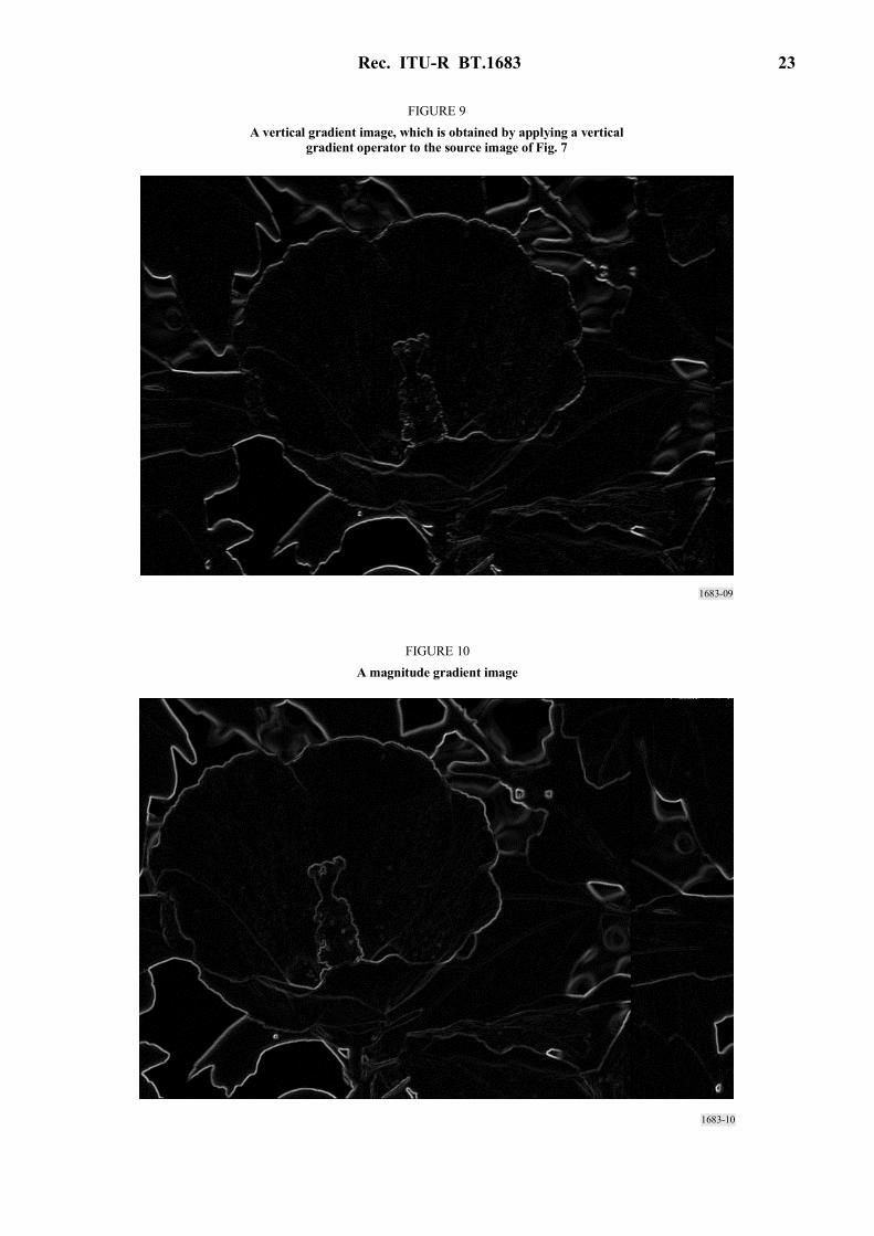
Figures 7-11 illustrate the above procedure. Figure 7 shows a source image. Figure 8 shows a horizontal gradient image ghorizontal(m,n), which is obtained by applying a horizontal gradient operator to the source image of Fig. 7. Figure 9 shows a vertical gradient image gvertical(m,n), which is obtained by applying a vertical gradient operator to the source image of Fig. 7. Figure 10 shows the magnitude gradient image (edge image) and Fig. 11 shows the binary edge image (mask image) obtained by applying thresholding to the magnitude gradient image of Fig. 10.

22 Rec. ITU-R BT.1683
1683-07
FIGURE 7A source image (original image)
1683-08
FIGURE 8A horizontal gradient image, which is obtained by applying a horizontal
gradient operator to the source image of Fig. 7
Rec. ITU-R BT.1683 23
1683-09
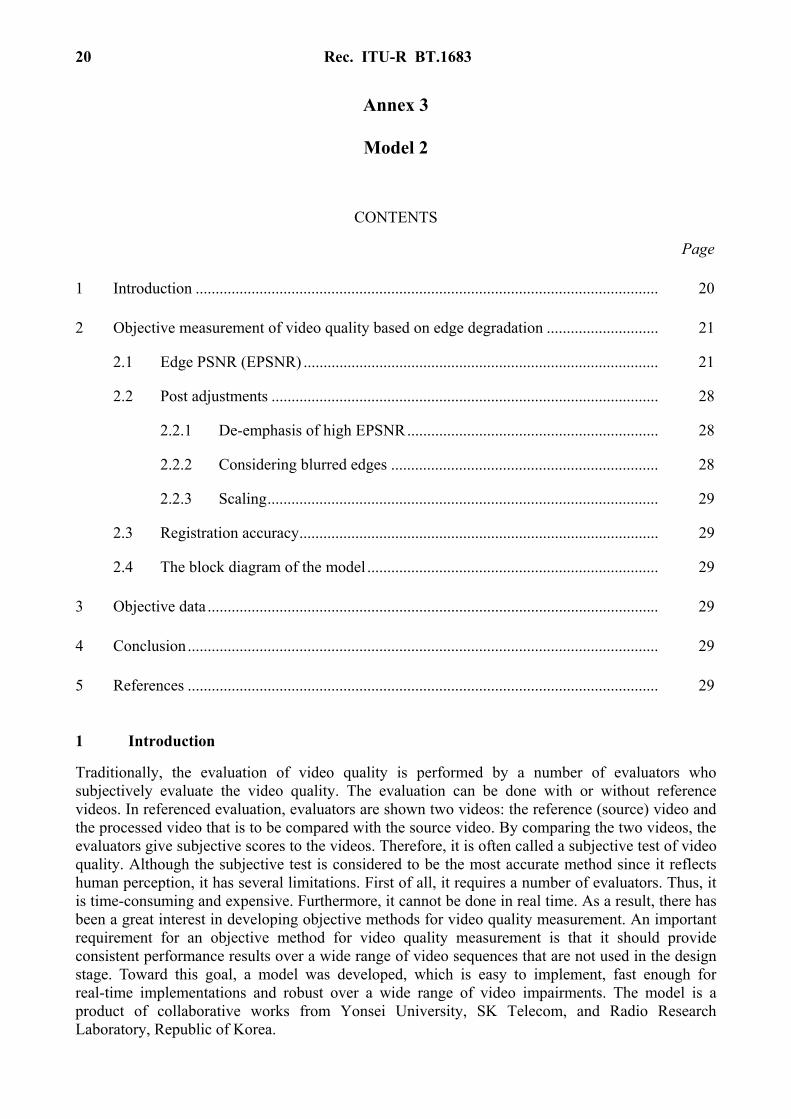
FIGURE 9A vertical gradient image, which is obtained by applying a vertical
gradient operator to the source image of Fig. 7
1683-10
FIGURE 10A magnitude gradient image

24 Rec. ITU-R BT.1683
1683-11
FIGURE 11A binary edge image (mask image) obtained by applying thresholding
to the magnitude gradient image of Fig. 10
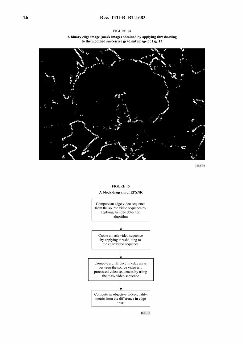
Alternatively, one may use a modified procedure to find edge areas. For instance, one may first apply a vertical gradient operator to the source image, producing a vertical gradient image. Then, a horizontal gradient operator is applied to the vertical gradient image, producing a modified successive gradient image (horizontal and vertical gradient image). Finally, a thresholding operation may be applied to the modified successive gradient image to find edge areas. In other words, pixels of the modified successive gradient image, which exceed a threshold value, are considered as edge areas. Figures 12-15 illustrate the modified procedure. Figure 12 shows a vertical gradient image gvertical(m,n), which is obtained by applying a vertical gradient operator to the source image of Fig. 7. Figure 13 shows a modified successive gradient image (horizontal and vertical gradient image), which is obtained by applying a horizontal gradient operator to the vertical gradient image of Fig. 12. Figure 14 shows the binary edge image (mask image) obtained by applying thresholding to the modified successive gradient image of Fig. 13.

Rec. ITU-R BT.1683 25
1683-12
FIGURE 12A vertical gradient image, which is obtained by applying a vertical
gradient operator to the source image of Fig. 7
1683-13
FIGURE 13A modified successive gradient image (horizontal and vertical gradient image),
which is obtained by applying a horizontal gradient operator to the vertical gradient image of Fig. 12
26 Rec. ITU-R BT.1683
1683-14
FIGURE 14A binary edge image (mask image) obtained by applying thresholding
to the modified successive gradient image of Fig. 13
1683-15
Compute an edge video sequencefrom the source video sequence by
applying an edge detectionalgorithm
Create a mask video sequenceby applying thresholding to
the edge video sequence
Compute a difference in edge areasbetween the source video and
processed video sequences by usingthe mask video sequence
Compute an objective video qualitymetric from the difference in edge
areas
FIGURE 15A block diagram of EPSNR

Rec. ITU-R BT.1683 27
It is noted that both methods can be understood as an edge detection algorithm. One may choose any edge detection algorithm depending on the nature of videos and compression algorithms. However, some methods may outperform other methods.
Thus, in the model, an edge detection operator is first applied, producing edge images (Figs. 10 and 13). Then, a mask image (binary edge image) is produced by applying thresholding to the edge image (Figs. 11 and 14). In other words, pixels of the edge image whose value is smaller than threshold, te, are set to zero and pixels whose value is equal to or larger than the threshold are set to a non-zero value. Figures 11 and 14 show examples of mask images. It is noted that this edge detection algorithm is applied to the source image. Although one may apply the edge detection algorithm to processed images, it is more accurate to apply it to the source images. Since a video can be viewed as a sequence of frames or fields, the above-stated procedure can be applied to each frame or field of videos. Since the model can be used for field-based videos or frame-based videos, the terminology “image” will be used to indicate a field or frame.
Next, differences between the source video sequence and processed video sequence, corresponding to non-zero pixels of the mask image are computed. In other words, the squared error of edge areas of the l-th frame is computed as follows:
0),(if),(),(1 1
2 ≠−=∑ ∑= =
jiRjiPjiSse lM
i
N
j
llle (75)
where: Sl(i,j) : l-th image of the source video sequence Pl(i,j) : l-th image of the processed video sequence Rl(i,j) : l-th image of the mask video sequence M : number of rows N : number of columns.
When the model is implemented, one may skip the generation of the mask video sequence. In fact, without creating the mask video sequence, the squared error of edge areas of the l-th frame is computed as follows:
el
M
i
N
j
llle tjiQjiPjiSse ≥−=∑ ∑
= =),(if),(),(
1 1
2 (76)
where: Ql(i,j) : l-th image of the edge video sequence te : threshold.
Although the mean squared error is used in equation (75) to compute the difference between the source video sequence and the processed video sequence, any other type of difference may be used. For instance, the absolute difference may be also used. In the model submitted to the VQEG Phase II test, te, was set to 260 and the modified edge detection algorithm was used with the Sobel operator.
This procedure is repeated for the entire video sequences and the edge mean squared error is computed as follows:
∑=
=L
l
lee se
Kmse
1
1 (77)
28 Rec. ITU-R BT.1683
where: L : number of images (frames or fields) K : total number of pixels of the edge areas.
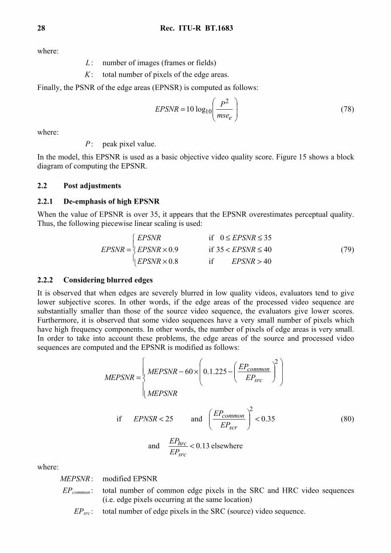
Finally, the PSNR of the edge areas (EPNSR) is computed as follows:
=
emsePEPSNR
210log10 (78)
where: P : peak pixel value.
In the model, this EPSNR is used as a basic objective video quality score. Figure 15 shows a block diagram of computing the EPSNR.
2.2 Post adjustments
2.2.1 De-emphasis of high EPSNR When the value of EPSNR is over 35, it appears that the EPSNR overestimates perceptual quality. Thus, the following piecewise linear scaling is used:
>×≤<×≤≤
=40if8.04035if9.0350if
EPSNREPSNREPSNREPSNREPSNREPSNR
EPSNR (79)
2.2.2 Considering blurred edges It is observed that when edges are severely blurred in low quality videos, evaluators tend to give lower subjective scores. In other words, if the edge areas of the processed video sequence are substantially smaller than those of the source video sequence, the evaluators give lower scores. Furthermore, it is observed that some video sequences have a very small number of pixels which have high frequency components. In other words, the number of pixels of edge areas is very small. In order to take into account these problems, the edge areas of the source and processed video sequences are computed and the EPSNR is modified as follows:
−×−
=
MEPSNR
EPEPMEPSNR
MEPSNR src
common2
225.1.060
35.0and25if2
<
<
scr
commonEP
EPEPNSR (80)
elsewhere13.0and <src
hrcEPEP
where: MEPSNR : modified EPSNR EPcommon : total number of common edge pixels in the SRC and HRC video sequences
(i.e. edge pixels occurring at the same location) EPsrc : total number of edge pixels in the SRC (source) video sequence.
Rec. ITU-R BT.1683 29
For some video sequences, EPsrc can be very small. If EPsrc is smaller than 10 000 pixels (about 10 000/240 = 41.7 pixels per frame for the 8 s 525 videos and about 10 000/200 = 50 pixels per frame for the 8 s 625 videos), the user may reduce threshold te in equation (76) by 20 until EPsrc is larger than or equal to 10 000 pixels. If EPsrc is smaller than 10 000 pixels even when te is reduced to 80, the post adjustment using equation (80) is not used. In this case, the EPSNR is computed using te = 60. If this option is taken, the user may delete the condition of EPhrc/EPsrc < 0.13 in equation (80).
2.2.3 Scaling
Next, scale objective scores are rescaled so that they will be between 0 (not distinguishable from the original video) and 1.
02.01 ×−= MEPSNRVQM (81)
This VQM is used as the objective score of the model.
2.3 Registration accuracy
The recommended registration accuracy for the model is a half-pixel accuracy in the interlaced videos, which is equivalent to a quarter-pixel accuracy in the progressive video format. The cubic spline interpolation [Lee et al., 1998] or better is strongly recommended to calculate sub-pixel values.
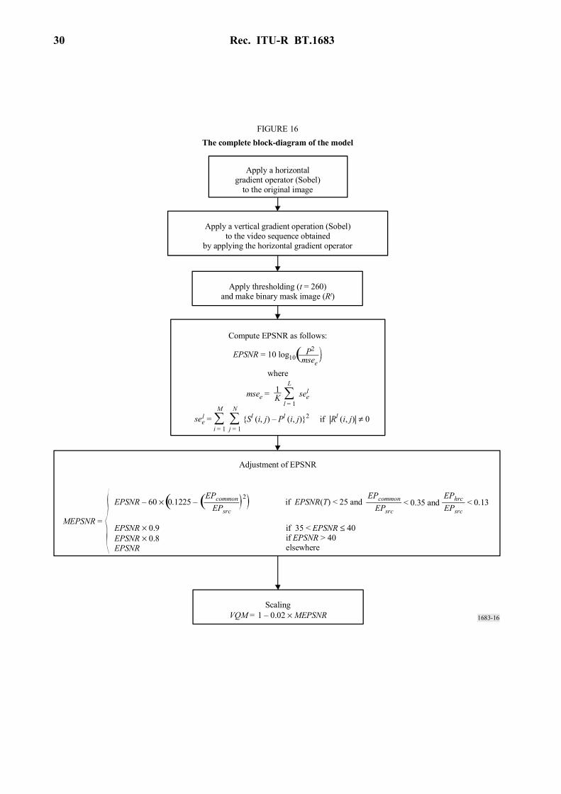
2.4 The block diagram of the model
Figure 16 shows the complete block diagram of the model.
3 Objective data
The model was applied to the VQEG Phase II video data1. However, after the model was submitted, registration and operator errors were found. The objective data presented in this Annex is the same data as in the VQEG Phase II Final Report. Consequently, when the method described in this Annex is properly implemented, the user may obtain different objective data from those of this Annex. Tables 7 to 8 show the objective data of the 525 and 625 video data sets.
4 Conclusion
A new model for objective measurement of video quality is proposed based on edge degradation. The model is extremely fast. Once the bit-map is generated, the model is several times faster than the conventional PSNR, providing a significant improvement. Therefore, the model is well suited to applications which require real-time video quality evaluation.
5 Reference
LEE C., EDEN M. and UNSER M., [1998] High quality image resizing using oblique projection operators. IEEE Trans. Image Processing, Vol. 5, 5, p. 679-692.
30 Rec. ITU-R BT.1683
1683-16
FIGURE 16The complete block-diagram of the model
Apply a horizontalgradient operator (Sobel)
to the original image
Apply a vertical gradient operation (Sobel)to the video sequence obtained
by applying the horizontal gradient operator
Apply thresholding (t = 260)and make binary mask image (Rl)
Compute EPSNR as follows:
where
EPSNR = 10 log10P2
msee(
msee =1K ∑
l = 1
L
see l
∑i = 1
M
Sl (i, j) – Pl (i, j)2 if |Rl (i, j)| ≠ 0see =l ∑j = 1
N
Adjustment of EPSNR
MEPSNR =EPSNR × 0.9EPSNR × 0.8EPSNR
EPSNR – 60 × 0.1225 – 2EPcommon
EPsrcif EPSNR(T) < 25 and < 0.35 and
EPcommonEPsrc
EPhrcEPsrc
< 0.13
if 35 < EPSNR ≤ 40if EPSNR > 40elsewhere
ScalingVQM = 1 – 0.02 × MEPSNR
( (

Rec. ITU
-R BT.1683
31
TABLE 7
The 525 VQM matrix (yonsei_1128c.exe)(1)
HRC SRC (image) 1 2 3 4 5 6 7 8 9 10 11 12 13 14
1 1 0.679 4 0.525 7 0.512 10 0.419
2 2 0.431 5 0.365 8 0.313 11 0.342
3 3 0.558 6 0.452 9 0.340 12 0.305
4 13 0.668 17 0.581 21 0.556 25 0.535
5 14 0.543 18 0.485 22 0.443 26 0.410
6 15 0.631 19 0.477 23 0.441 27 0.411
7 16 0.467 20 0.415 24 0.376 28 0.346
8 29 0.787 35 0.734 41 0.740 47 0.551 53 0.520 59 0.537
9 30 0.848 36 0.559 42 0.723 48 0.495 54 0.462 60 0.465
10 31 0.552 37 0.449 43 0.542 49 0.352 55 0.308 61 0.377
11 32 0.610 38 0.628 44 0.633 50 0.475 56 0.471 62 0.498
12 33 0.576 39 0.539 45 0.577 51 0.470 57 0.436 63 0.448
13 34 0.554 40 0.569 46 0.517 52 0.399 58 0.382 64 0.412
(1) After the model was submitted, registration and operator errors were found. The objective data presented in this Annex is the same data as in the VQEG Phase II Final Report. Consequently, when the method described in this Annex is properly implemented, the user may obtain different objective data from those of Table 7.
32
Rec. ITU
-R BT.1683
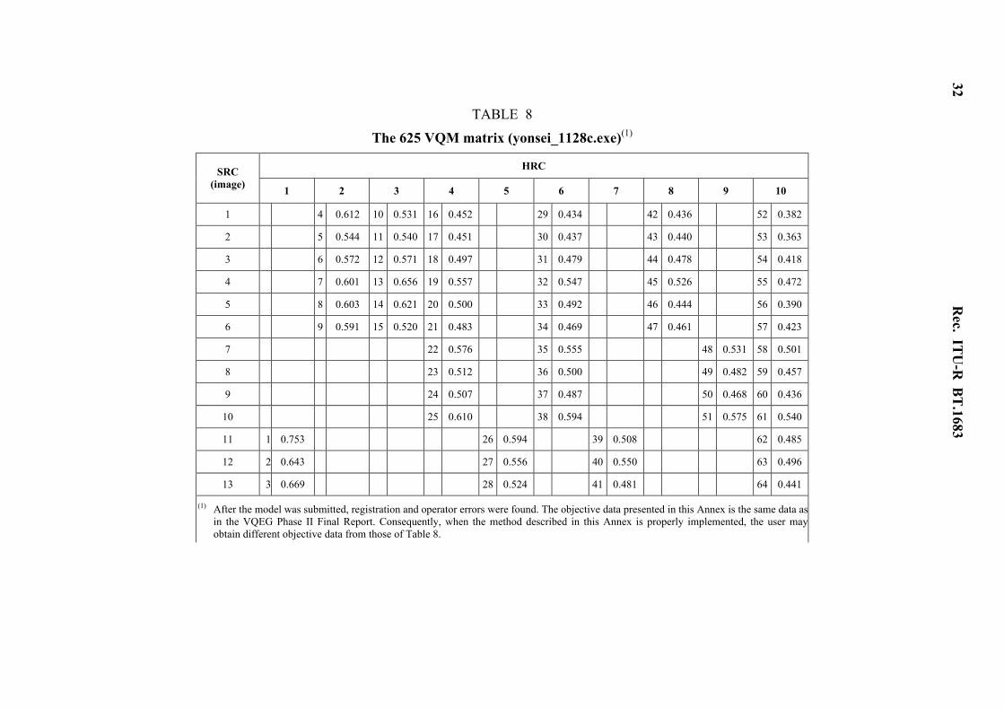
TABLE 8
The 625 VQM matrix (yonsei_1128c.exe)(1)
HRC SRC (image) 1 2 3 4 5 6 7 8 9 10
1 4 0.612 10 0.531 16 0.452 29 0.434 42 0.436 52 0.382
2 5 0.544 11 0.540 17 0.451 30 0.437 43 0.440 53 0.363
3 6 0.572 12 0.571 18 0.497 31 0.479 44 0.478 54 0.418
4 7 0.601 13 0.656 19 0.557 32 0.547 45 0.526 55 0.472
5 8 0.603 14 0.621 20 0.500 33 0.492 46 0.444 56 0.390
6 9 0.591 15 0.520 21 0.483 34 0.469 47 0.461 57 0.423
7 22 0.576 35 0.555 48 0.531 58 0.501
8 23 0.512 36 0.500 49 0.482 59 0.457
9 24 0.507 37 0.487 50 0.468 60 0.436
10 25 0.610 38 0.594 51 0.575 61 0.540
11 1 0.753 26 0.594 39 0.508 62 0.485
12 2 0.643 27 0.556 40 0.550 63 0.496
13 3 0.669 28 0.524 41 0.481 64 0.441
(1) After the model was submitted, registration and operator errors were found. The objective data presented in this Annex is the same data as in the VQEG Phase II Final Report. Consequently, when the method described in this Annex is properly implemented, the user may obtain different objective data from those of Table 8.
Rec. ITU-R BT.1683 33
Annex 4
Model 3
CONTENTS
Page
1 Introduction .................................................................................................................... 33
2 General description of the IES system ........................................................................... 34
3 Correction of offset and gain .......................................................................................... 36
3.1 Temporal offset................................................................................................... 36
3.2 Spatial offset ....................................................................................................... 37
3.3 Gain..................................................................................................................... 37
4 Image segmentation........................................................................................................ 38
4.1 Plane regions....................................................................................................... 38
4.2 Edge regions ....................................................................................................... 38
4.3 Texture regions ................................................................................................... 40
5 Objective measurement .................................................................................................. 40
6 Database of impairment models ..................................................................................... 40
7 Estimation of impairment models .................................................................................. 41
7.1 Computation of Wi .............................................................................................. 41
7.2 Computation of Fi and Gi.................................................................................... 42
8 References ...................................................................................................................... 43
Annex 4a .................................................................................................................................. 44
1 Introduction
This Annex presents a methodology for video quality assessment using objective parameters based on image segmentation. Natural scenes are segmented into plane, edge and texture regions, and a set of objective parameters are assigned to each of these contexts. A perceptual-based model that predicts subjective (Recommendation ITU-R BT.500 and Recommendation ITU-R BT.802 – Test pictures and sequences for subjective assessments of digital codecs conveying signals produced according to Recommendation ITU-R BT.601) ratings is defined by computing the relationship between objective measures and results of subjective assessment tests, applied to a set of natural

34 Rec. ITU-R BT.1683
scenes processed by MPEG-2 video codecs. In this model, the relationship between each objective parameter processed by several compression systems (like MPEG-2 and MPEG-1 codecs) and the subjective impairment level is approximated by a logistic curve, resulting in an estimated impairment level for each parameter. The final result is achieved through a linear combination of estimated impairment levels, where the weight of each impairment level is proportional to its statistical reliability.
In § 2, a general description of CPqD-IES (image evaluation based on segmentation) system is presented. In § 3, the steps to register spatial and temporal misalignments, as well as the correction of gain are described. In § 4, the algorithm to segment images into plane, edge and texture regions is explained. In § 5, the objective measurement carried out over each region and each image component is described. Section 6 describes the way that the database of impairment models was constructed. The calculations of the parameters also are described in this Section. Section 7 describes the estimation of video quality rating from the parameters in database of impairment models. Annex 4a presents results of video quality rating (VQR) estimated during VQEG Phase II tests1.
2 General description of the IES system
Figure 17 presents an overview of the CPqD-IES algorithm for natural scenes. Each natural scene is represented by one original (reference) scene O and one impaired scene I, which results from a codec operation applied to O. Offset and gain corrections are applied to I in order to create a corrected impaired scene I', such that each frame f of I' corresponds to the reference frame f of O for f = 1, 2, ..., n (§ 3.2).
Input scenes I and O to the CPqD-IES algorithm are in YCbCr4:2:2 format according to Recommendation ITU-R BT.601 – Studio encoding parameters of digital television for standard 4:3 and wide-screen 16:9 aspect ratios.
The Y component of each image frame f of O is segmented into three categories: texture, edge, and plane regions (§ 4). One objective measure is computed based on the difference between the corresponding frames of O and I', for each of these contexts and for each image component YCbCr, forming a set of 9 objective measures m1, m2, ..., m9 for each image frame f (§ 5). Each objective measure mi, i = 1, 2, ..., 9, produces a contextual impairment level Li based on its impairment estimation model, which is given by:
1/100
+=
iG
i
ii m
FL (82)
where Fi and Gi are two parameters computed (§ 7) based on a database of impairment models (Section 6), spatial S and temporal F attributes (§ 5), and on the objective measures mi
(420) and mi
(CIF) for frame f, resulting from the codec operations CD420 and CDCIF applied to O (§ 7). The two reference impairment codecs, CD420 (coder/decoder MPEG-2 4:2:0) and CDCIF (coder/decoder MPEG-1 CIF), are totally based on the routines extracted directly from MPEG2 (ITU-T Recommendation H.262 – Information technology – Generic coding of moving pictures and associated audio information: Video.) and MPEG1 [ISO/IEC, 1992], available at http://www.mpeg.org/MPEG/MSSG. In the current implementation of the CPqD-IES algorithm, these routines operate in intra mode using a fix quantization step of 16. It is important to note that CD420 and CDCIF do not introduce offset and gain differences with respect to O.

Rec. ITU-R BT.1683 35
1683-17
FIGURE 17General overview of the CPqD-IES algorithm
VQR estimation
Estimation of the contextual impairment models of the input scene
Temporal offsetcorrection
Spatial offsetcorrection
YCbCr gaincorrection
Segmentation
Objectivemeasurements
Objectivemeasurements
CD420 CDCIF
Objectivemeasurements
I' (Correctedimpaired scene)
Edge, plane,texture regions
I(420) I(CIF)
mi(420) mi
(CIF)mi
Fi, Gi, Wi
VQR
O (Input original scene)
I (Input impaired scene)
Database ofimpairment models
and measures
Fij, Gij, Wij
mij, Sj, Tj
CIF: common intermediate format
The video quality rate VQRf of frame f is obtained by linear combination of the contextual impairment levels Li, i = 1, 2, ..., 9, as follows:
9
1∑=
=i
iif LWVQR (83)
where Wi is the weight of the impairment level Li for this particular natural scene, which is computed as described in § 7.
Now, the sequence of values VQR1, VQR2, ... VQRn is transformed by a median filter of size 3 into another sequence VQR'1, VQR'2, ... VQR'n, by excluding the median value computation within the 1-neighbourhood of VQR1 and VQRn. During the median filtering, the algorithm avoids repetition of two consecutive median values. That is, if the median value VQR'f–1 computed within the
36 Rec. ITU-R BT.1683
1-neighbourhood of VQRf is equal to the median value VQR'f–2, computed within the 1-neighbourhood of VQRf–1, then the algorithm chooses VQR'f–1 as the minimum value computed within the 1-neighbourhood of VQRf. This algorithm can be described as follows.
1) For each f from 2 to n – 1, do
2) Compute med, the median value among VQRf–1 , VQRf , VQRf+1
3) If med = VQR'f–2 then
4) Compute VQR'f–1 as the minimum value among VQRf–1 , VQRf , VQRf+1
5) Else
6) VQR'f–1 ← med.
The final VQR is then the average of the VQRf' values.
.2
1 2
1∑−
=′
−=
n
ffRVQ
nVQR (84)
Equations (82), (83) and the above algorithm describe the process to estimate the VQR from the contextual impairment models Fi , Gi ,Wi and the objective measures mi, i = 1, 2, ..., 9. The next sections complete the description of the method by presenting the details inside the remaining blocks of Fig. 17.
3 Correction of offset and gain
3.1 Temporal offset
The temporal offset, dt, is an integer ranging from –2 to 2. Input scenes with temporal offsets out of this range are not considered. Let Idt be the impaired scene I with a displacement of f frames. A dissimilarity coefficient between O and each displaced scene Idt is calculated. The displacement with lowest dissimilarity coefficient is used as temporal offset, and the output Idt is then I displaced by this offset for the next computation. The dissimilarity coefficient between O and Idt is obtained as described below, where n is the number of frames in the temporal intersection between them:
1) ξT ← 0
2) For each f from 1 to n, do
3) Compute Sb
4) Compute bS ′
5) Compute Db
6) Compute µ, the mean value of the pixels in Db
7) ξT ← ξT +(µ/n)
8) Return ξT (dissimilarity coefficient between O and Idt).
Where:
Sb : magnitude of the Sobel’s gradient of the component Y of the f-th frame of O S'b : magnitude of the Sobel’s gradient of the component Y of the f-th frame of Idt
Db : pixel-wise absolute difference between Sb and .bS′
Rec. ITU-R BT.1683 37
3.2 Spatial offset
The spatial offset (dx, dy) is one of the following integer horizontal and vertical displacements dx = −6, –5, ... 6 and dy = –6, –5, ..., 6. Consider Idx, dy the impaired scene Idt with all frames displaced by (dx, dy) pixels. A dissimilarity coefficient between O and Idx, dy is calculated. The spatial displacement with lowest dissimilarity is used as spatial offset, and the output Idx, dy is then Idt displaced by this offset for the next computation.
The dissimilarity between O and Idx, dy is described below:
1) ξS ← 0 ; c ← 0 2) For each f from 1 to n, do 3) For x from x0 to (x0 + w/4) do 4) For y from y0 to (y0 + h/4) do
5) ξS ← ξS + |Y(4x,4y) – Y'(4x + dx, 4y + dy)| + + |Cb(4x,4y) – Cb'(4x + dx, 4y + dy)| + + |Cr(4x,4y) – Cr'(4x + dx, 4y + dy)|
6) c ← c + 3
7) ξS ← ξS /c
8) Return ξS (dissimilarity coefficient between O and Idx, dy).
Where: w × h : size of the intersection area between O and Idx, dy Y(x, y), Cb(x, y), Cr(x, y) : values in the image components of a frame f of O for a pixel (x, y) Y'(x + dx, y + dy) Cb'(x + dx, y + dy) Cr'(x + dx, y + dy) : values in the image components of a frame f of Idx, dy for a pixel
(x + dx, y + dy).
3.3 Gain
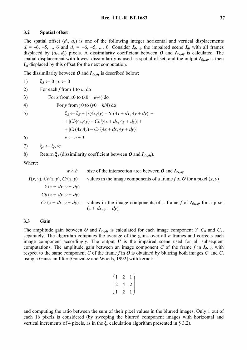
The amplitude gain between O and Idx, dy is calculated for each image component Y, CB and CR, separately. The algorithm computes the average of the gains over all n frames and corrects each image component accordingly. The output I' is the impaired scene used for all subsequent computations. The amplitude gain between an image component C of the frame f in Idx, dy with respect to the same component C of the frame f in O is obtained by blurring both images C' and C, using a Gaussian filter [Gonzalez and Woods, 1992] with kernel:
121242121
and computing the ratio between the sum of their pixel values in the blurred images. Only 1 out of each 16 pixels is considered (by sweeping the blurred component images with horizontal and vertical increments of 4 pixels, as in the ξs calculation algorithm presented in § 3.2).
38 Rec. ITU-R BT.1683
4 Image segmentation
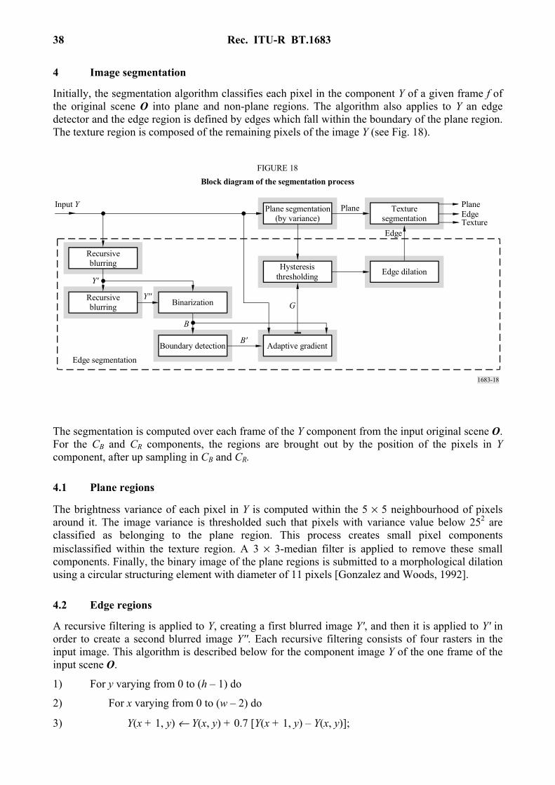
Initially, the segmentation algorithm classifies each pixel in the component Y of a given frame f of the original scene O into plane and non-plane regions. The algorithm also applies to Y an edge detector and the edge region is defined by edges which fall within the boundary of the plane region. The texture region is composed of the remaining pixels of the image Y (see Fig. 18).
1683-18
Y'
Y''
B
B'
G
Plane
Edge
PlaneEdgeTexture
Plane segmentation(by variance)
Texturesegmentation
Edge dilationHysteresisthresholding
Adaptive gradientBoundary detection
BinarizationRecursiveblurring
Recursiveblurring
Input Y
FIGURE 18Block diagram of the segmentation process
Edge segmentation
The segmentation is computed over each frame of the Y component from the input original scene O. For the CB and CR components, the regions are brought out by the position of the pixels in Y component, after up sampling in CB and CR.
4.1 Plane regions
The brightness variance of each pixel in Y is computed within the 5 × 5 neighbourhood of pixels around it. The image variance is thresholded such that pixels with variance value below 252 are classified as belonging to the plane region. This process creates small pixel components misclassified within the texture region. A 3 × 3-median filter is applied to remove these small components. Finally, the binary image of the plane regions is submitted to a morphological dilation using a circular structuring element with diameter of 11 pixels [Gonzalez and Woods, 1992].
4.2 Edge regions
A recursive filtering is applied to Y, creating a first blurred image Y', and then it is applied to Y' in order to create a second blurred image Y''. Each recursive filtering consists of four rasters in the input image. This algorithm is described below for the component image Y of the one frame of the input scene O.
1) For y varying from 0 to (h – 1) do
2) For x varying from 0 to (w – 2) do
3) Y(x + 1, y) ← Y(x, y) + 0.7 [Y(x + 1, y) – Y(x, y)];

Rec. ITU-R BT.1683 39
4) For y varying from 0 to (h – 1) do 5) For x varying from (w – 1) to 1 do 6) Y(x – 1, y) ← Y(x, y) + 0.7 [Y(x – 1, y) – Y(x, y)]; 7) For x varying from 0 to (w – 1) do 8) For y varying from 0 to (h – 2) do 9) Y(x, y + 1) ← Y(x, y) + 0.7 [Y(x, y + 1) – Y(x, y)]; 10) For x varying from 0 to (w – 1) do 11) For y varying from (h – 1) to 1 do 12) Y(x, y + 1) ← Y(x, y) + 0.7 [Y(–1) – Y(x, y)]; 13) Save image Y in image Y'.
Where: Y(x, y) : brightness of the pixel (x, y) h : number of lines in Y w : number of columns in Y.
The second application of the above algorithm will create Y''. A binary image B is created from Y' and Y'':
≥
=otherwise 0
),(),( if 1),(
yxY''yxY'yxB (85)
After that, the algorithm identifies the boundary pixels of the regions in B with pixel-value 1 by creating a second binary image B':
∈==
=′otherwise 0
),(),( pixelany for 0 ),( and 1 if 1),( 8 yxΝy'x'y'x'BB(x,y)
yxB (86)
where Ν8(x, y) is the set of pixels (x', y') within the 3 × 3 neighbourhood of (x, y) (i.e. its 8 neighbours).
An adaptive gradient filter is applied to Y restricted to the pixels where B'(x, y) = 1:
=′µ−µ
=otherwise 0
1),( if ),( 01 yxB
yxG (87)
where:
1),(such that),(),( allfor ),',( of mean value : 81 =∈µ y'x'ByxΝy'x'yx'Y
.0),(such that),(),( allfor ),,( of mean value : 80 =∈µ y'x'ByxΝy'x'y'x'Y
Note that, the algorithm uses B instead of B' to compute the mean values µ1 and µ0.
A hysteresis thresholding [Trucco and Verri, 1998] is applied to G restricted to pixels which have been classified in § 4.1 as belonging to the plane region. The lower threshold is 30 and the upper threshold is 40. The algorithm first identifies the pixels in G, such that G(x, y) > 40, and then it applies a region growing algorithm along the lines of G by using these pixels as seeds and by restricting the growth to pixels in the same line whose G(x, y) > 30. All 4-connected pixel components with less than 6 pixels are eliminated from this result. The final binary image is dilated by a circular structuring element with diameter of 5 pixels ignoring the restriction to the plane region. The pixels with value 1 in this dilation are classified as belonging to the edge region.

40 Rec. ITU-R BT.1683
4.3 Texture regions
The texture region consists of the pixels in Y which were neither classified as belonging to the edge region nor to the plane region in the above sections.
5 Objective measurement
Consider Sb, the image of magnitude of the Sobel’s gradient computed for a given component (Y, CB or CR) of a given frame f of the original scene O, and ,bS′ the image of magnitude of the Sobel’s gradient for the same component of frame f of the impaired scene I'. The image Db of the pixel-wise absolute difference between Sb and bS ′ is computed and the region ℜ of pixels in Db that belong to a given context (plane, edge or texture) is considered. The absolute Sobel's difference (ASD) for this image component and context is defined as the average of the pixel values in Db restricted to ℜ.
This procedure produces a set of nine objective measures m1, m2, ..., m9 for each image frame f, f = 1, 2, ..., n, considering all three contexts and three image components.
The same process is applied to create objective measures m1(420), m2
(420), ..., m9(420) and m1
(CIF), m2
(CIF), ..., m9(CIF), for the frame f with respect to the MPEG-2 4:2:0 and MPEG-1 CIF CODEC
operations over O (see Fig. 17). These measures are used as references together with spatial S and temporal T attributes in order to determine the contextual impairment model for I' (§ 7). The temporal attribute T is the mean value of the pixel-wise absolute difference between the segmentations of the frames f and f – 1, normalized within [0,1]. The spatial attribute S is defined as the ratio m7
(CIF)/m7(420), normalized in [0,1], where m7
(CIF) and m7(420) are the corresponding ASDs
for the texture region in the component Y of the frame f.
6 Database of impairment models
The IES system uses a database of impairment models for scenes different from the reference scene O in order to estimate the video quality rate of I'. This database consists of information about twelve 60 Hz scenes representing different degrees of motion (dynamic and static scenes), nature (real and synthetic scenes), and context (amount of texture, plane, and edge pixels). This database was created as follows.
The mean values of the objective measures jjj mmm ,9,2,1 ,...,, , )420(,9
)420(,2
)420(,1 ,...,, jjj mmm , and )(
,9)(
,2)(
,1 ,...,, CIFj
CIFj
CIFj mmm were computed over the frames of each scene j, j = 1, 2, ..., 12. The
values of Sj and Tj were calculated as the average of the spatial and temporal attributes, computed as described in § 5, over frames of each scene j. All impaired scenes of the database were also submitted to subjective evaluation, obtaining a subjective impairment level ,jSL normalized between 0% and 100% for each scene j.
According to equation (82), each objective measure mi,j, i = 1, 2, ..., 9 and j = 1, 2, ..., 12, is related to a contextual impairment level Li,j. The values of Fi,j and Gi,j in equation (82) were found for each scene j by minimizing the expectation of the mean square error ][ 2),( jiLjLSE − . Moreover, the values of Wi,j in equation (83) were computed in order to minimize the expectation of the mean square error
−∑
=
29
1,,
ijijij LWLSE (88)

Rec. ITU-R BT.1683 41
Finally, the database of impairment models consists of nine sets jjjijiji TSWGF ,,,, ,,, , i = 1, 2, ..., 9, of parameters for each scene j, j = 1, 2, ..., 12. Table 9 contains the values of jS and
jT to calculate the attributes jijiji WGF ,,, ,, .
7 Estimation of impairment models
The contextual impairment models for a given frame f of I' consist of the parameters Fi, Gi, Wi of equations (82) and (83), i = 1, 2, ..., 9. This section describes how to compute these parameters using the I(420) and I(CIF) impaired scenes as references.
7.1 Computation of Wi
The contextual local distances Di,j between a frame f of the impaired scenes, I(420) and I(CIF), and each scene j of the database are defined as:
( )( )
( )( )
+=
+=
+=
+=
ji
ji
ji
ji
GCIFiji
CIFji
Gijiji
GCIFiji
CIFji
Gijiji
mFL
mFL
mFL
mFL
,
,
,
,
)(,
)(,
)420(,
)420(,
)(,
)(,
)420(,
)420(,
/1/100
/1/100
/1/100
/1/100
(89)
TABLE 9
Temporal T and spatial S attributes
Scene j T (temporal) SY (spatial Y) SCb (spatial CB) SCr (spatial CR)
1 27.01 36.79 25.20 38.01 2 25.33 26.08 5.93 67.99 3 45.54 60.97 10.28 28.75 4 36.40 30.47 6.46 63.07 5 32.02 72.50 11.72 15.78 6 12.63 84.22 2.85 12.94 7 28.38 61.53 11.08 27.39 8 10.19 46.08 5.45 48.47 9 0.01 5.89 5.07 89.03
10 7.26 4.75 2.00 93.25 11 7.60 69.16 9.41 21.43 12 14.27 69.61 3.89 26.50

42 Rec. ITU-R BT.1683
)420(, jiL and are estimated impairment levels of the input scene O, calculated with parameters jiF ,
and jiG , , in the context i, of the scenes j from the database.
−+−= )420(
,)(
,)420(
,)420(
,, .21
jiCIFjijijiji LLLLD (90)
The algorithm finds the set Ω of the six closest scenes of the database based on the Di,j distance and defines Wi,j as:
Ω∈
=otherwise 0
) (scene if 1 kak (91)
∑=
−
−= 12
1
1,
1,
,
kkik
jijji
Da
DaW (92)
Consider now that i = 1, 2, ..., 9 ≡ (plane, Y), (plane, CB), (plane, CR), (edge, Y), (edge, CB), (edge, CR), (texture, Y), (texture, CB), (texture, CR), where (plane, C), (edge, C) and (texture, C) represent the plane, edge, and texture regions of the image component C, C = Y, CB, CR.
Let u = texture, edge, plane and v = Y, CB, CR, the values Wi, i = 1, 2, ..., 9, are computed as:
∑
∑
++=τ
=
=κ
==
u CuCuYu
ivu
jjijii
RBEEE
Yv
WDE
,,,
,
12
1,,
11211
otherwise 21
if 1
i
ii E
W 1⋅τκ= (93)
7.2 Computation of Fi and Gi
The contextual impairment levels )420(iL and )(CIF
iL of frame f for CD420 and CDSIF are computed as:
∑=
⋅γ
=12
1
)420(,,
)420( 1
jjijii LWL (94)
∑=
⋅γ
=12
1
)(,,
)( 1
j
CIFjiji
CIFi LWL (95)

Rec. ITU-R BT.1683 43
where γ is a factor restricted into [1/2, 2], which is computed based on the vector distances, Dj, between the spatial and temporal attributes (see § 5), ),( jj TS and ),( jj TS , of the input scene and each database scene, respectively.
( ) 22 )( jjj TTSSD −+−= (96)
ba
STSTb
STTSwa
D
Dw
j
jj
jjj
kk
jj
−+=γ
−⋅−+=
−⋅−+
⋅=
=
∑
∑
=
=
−
−
1
21)1(
2
21)1(
2
22
12
1
22
12
1
1
1
(97)
The parameters Fi and Gi are finally obtained by solving the equation system below:
+=
iG
i
ii
m
FL )420(
)420( 1/100 (98)
+=
iG
CIFi
iCIFi
m
FL )(
)( 1/100 (99)
8 References
GONZALEZ, R. C. and WOODS, R. E. [1992] Digital Image Processing. Addison-Wesley.
ISO/IEC[1992] Standard ISO/IEC 11172 – Information technology – Coding of moving pictures and associated audio for digital storage media up to about 1.5 Mbit/s.
TRUCCO, E. and VERRI, A. [1998] Introductory Techniques for 3-D Computer Vision. Prentice-Hall.

44 Rec. ITU-R BT.1683
Annex 4a
Objective results in VQEG-Phase II tests
TABLE 10
625/60 raw objective data matrix
TABLE 11
525/60 raw objective data matrix
HRC SRC
1 2 3 4 5 6 7 8 9 10 1 0.6343 0.5083 0.287 0.2461 0.1951 0.1548 2 0.5483 0.5966 0.3649 0.3185 0.2668 0.1597 3 0.5998 0.6299 0.4551 0.3927 0.3428 0.2553 4 0.6055 0.8159 0.5684 0.5397 0.4158 0.309 5 0.6483 0.7268 0.4358 0.418 0.2874 0.1898 6 0.6146 0.4908 0.3671 0.3139 0.2562 0.2107 7 0.5865 0.5536 0.4841 0.3917 8 0.5023 0.457 0.3949 0.3158 9 0.4563 0.3927 0.3399 0.2667
10 0.7036 0.6511 0.6025 0.5083 11 0.8124 0.6374 0.3205 0.3221 12 0.7015 0.547 0.4997 0.3922 13 0.709 0.5098 0.4199 0.3298
HRC SRC
1 2 3 4 5 6 7 8 9 10 11 12 13 14 1 0.5472 0.3698 0.3429 0.1918
2 0.5075 0.226 0.1028 0.0789
3 0.3549 0.127 0.058 0.0339
4 0.6062 0.419 0.36 0.3108
5 0.4444 0.2957 0.2152 0.1635
6 0.6098(1) 0.3462 0.2546 0.1967
7 0.2404 0.135 0.0864 0.0609
8 0.8666 0.7554 0.6944 0.7048 0.6685 0.494
9 0.8896 0.7134 0.6204 0.6504 0.6246 0.2326
10 0.8776 0.6419 0.4788 0.6392 0.6237 0.1571
11 0.8623 0.7207 0.5719 0.5619 0.5796 0.3012
12 0.8262 0.6193 0.5139 0.5391 0.4946 0.1992
13 0.8223 0.5609 0.3454 0.437 0.4246 0.215
(1) The SRC = 6, HRC = 5 value was taken out of the analysis because it exceeded the temporal registration requirements of the VQEG test plan.

Rec. ITU-R BT.1683 45
Annex 5
Model 4
This Annex provides a full functional description of the NTIA VQM and its associated calibration techniques.
The calibration algorithms described in this Annex are sufficient to ensure proper operation of the NTIA video quality estimator. In general, these algorithms have a spatial registration accuracy of plus or minus 1/2 pixel and a temporal registration accuracy of plus or minus one interlaced field.
CONTENTS
Page
1 Introduction .................................................................................................................... 47
2 Normative reference ....................................................................................................... 47
3 Definitions ...................................................................................................................... 47
4 Overview of the VQM computation............................................................................... 51
5 Sampling......................................................................................................................... 51
5.1 Temporal indexing of original and processed video files................................... 52
5.2 Spatial indexing of original and processed video frames ................................... 53
5.3 Specifying rectangular sub-regions .................................................................... 54
5.4 Considerations for video sequences longer than 10 s ......................................... 55
6 Calibration ...................................................................................................................... 55
6.1 Spatial registration .............................................................................................. 56
6.1.1 Overview.............................................................................................. 56
6.1.2 Interlace issues ..................................................................................... 57
6.1.3 Required inputs to the spatial registration algorithm ........................... 58
6.1.4 Sub-algorithms used by the spatial registration algorithm................... 59
6.1.5 Spatial registration using arbitrary scenes............................................ 60
6.1.6 Spatial registration of progressive video.............................................. 65
6.2 Valid region ........................................................................................................ 66
6.2.1 Core valid region algorithm ................................................................. 66
6.2.2 Applying the core valid region algorithm to a video sequence............ 67
6.2.3 Comments on valid region algorithm................................................... 68

46 Rec. ITU-R BT.1683
Page
6.3 Gain and offset.................................................................................................... 68
6.3.1 Core gain and level offset algorithm.................................................... 68
6.3.2 Using scenes......................................................................................... 69
6.3.3 Applying gain and level offset corrections .......................................... 71
6.4 Temporal registration.......................................................................................... 71
6.4.1 Frame-based algorithm for estimating variable temporal delays between original and processed video sequences ................................ 72
6.4.2 Applying temporal registration correction........................................... 75
7 Quality features .............................................................................................................. 76
7.1 Introduction......................................................................................................... 76
7.1.1 S-T regions........................................................................................... 76
7.2 Features based on spatial gradients..................................................................... 78
7.2.1 Edge enhancement filters ..................................................................... 79
7.2.2 Description of features fSI13 and fHV13 ................................................... 79
7.3 Features based on chrominance information ...................................................... 81
7.4 Features based on contrast information .............................................................. 82
7.5 Features based on ATI ........................................................................................ 82
7.6 Features based on the cross product of contrast and ATI ................................... 82
8 Quality parameters.......................................................................................................... 83
8.1 Introduction......................................................................................................... 83
8.2 Comparison functions......................................................................................... 83
8.2.1 Error ratio and logarithmic ratio .......................................................... 84
8.2.2 Euclidean distance................................................................................ 84
8.3 Spatial collapsing functions................................................................................ 85
8.4 Temporal collapsing functions ........................................................................... 85
8.5 Non-linear scaling and clipping.......................................................................... 87
8.6 Parameter naming convention ............................................................................ 88
8.6.1 Example parameter names ................................................................... 90
9 General model................................................................................................................. 92
10 References ...................................................................................................................... 93
Annex 5a .................................................................................................................................. 93

Rec. ITU-R BT.1683 47
1 Introduction
This Annex provides a complete technical description of the NTIA General Model and its associated calibration techniques (e.g. estimation and correction of spatial registration, temporal registration, and gain/offset errors). The General Model is proponent H in the VQEG Phase II Full Reference Television tests. The General Model was designed to be a general purpose VQM for video systems that span a very wide range of quality and bit rates. Extensive subjective and objective tests were conducted to verify the performance of the General Model before it was submitted to the VQEG Phase II test. While the VQEG Phase II tests only evaluated the performance of the General Model on MPEG-2 and ITU-T Recommendation H.263 video systems, the General Model should work well for many other types of coding and transmission systems.
The calibration algorithms described in this Annex are sufficient to ensure proper operation of the video quality estimator. In general, these algorithms have a spatial registration accuracy of plus or minus 1/2 pixel and a temporal registration accuracy of plus or minus one interlaced field.
The General Model and its associated automatic calibration techniques have been completely implemented in user friendly software. This software is available to all interested parties via a no-cost evaluation license agreement (see www.its.bldrdoc.gov/n3/video/vqmsoftware.htm for more information).
2 Normative reference
Recommendation ITU-R BT.601 – Studio encoding parameters of digital television for standard 4:3 and wide-screen 16:9 aspect ratios.
3 Definitions
4:2:2 – A Y, Cb, Cr image sampling format where chrominance planes (Cb and Cr) are sampled horizontally at half the luminance (Y) plane’s sampling rate. See Recommendation ITU-R BT.601 (see Section 2).
Absolute temporal information (ATI): A feature derived from the absolute value of temporal information images that are computed as the difference between successive frames in a video clip. ATI quantifies the amount of motion in a video scene. See § 7.5 for the precise mathematical definition.
Big YUV: The binary file format used for storing clips that have been sampled according to Recommendation ITU-R BT.601. In the Big YUV format, all the video frames for a scene are stored in one large binary file, where each individual frame conforms to Recommendation ITU-R BT.601 sampling. The Y represents the luminance channel information, the U represents the blue colour difference channel (i.e. CB in Recommendation ITU-R BT.601), and the V represents the red colour difference channel (i.e. CR in Recommendation ITU-R BT.601). The pixel ordering in the binary file is the same as that specified in SMPTE 125M [SMPTE, 1995a]. The full specification of the Big YUV file format is given in Section 5 and software routines for reading and displaying Big YUV files are given in [Pinson and Wolf, 2002].
Clip: Digital representation of a scene that is stored on computer media.
Clip VQM: The VQM of a single clip of processed video.
Chrominance (C, CB, CR): The portion of the video signal that predominantly carries the colour information (C), perhaps separated further into a blue colour difference signal (CB) and a red colour difference signal (CR).
Codec: Abbreviation for a coder/decoder or compressor/decompressor.

48 Rec. ITU-R BT.1683
Common intermediate format (CIF): A video sampling structure used for video teleconferencing where the luminance channel is sampled at 352 pixels by 288 lines (see ITU-T Recommendation H.261 – Video codec for audiovisual services at p × 64 kbit/s.).
Feature: A quantity of information associated with, or extracted from, a spatial-temporal sub-region of a video stream (either an original video stream or a processed video stream).
Field: One half of a frame, containing all of the odd or even lines.
Frame: One complete television picture.
Frames per second (FPS): The number of original frames per second transmitted by the video system under test. For instance, an NTSC video system transmits approximately 30 fps.
Gain: A multiplicative scaling factor applied by the hypothetical reference circuit (HRC) to all pixels of an individual image plane (e.g. luminance, chrominance). Gain of the luminance signal is commonly known as contrast.
General Model: The video quality model, or VQM, that is the subject of this Annex 5. The General Model was submitted to the phase II tests performed by the Video Quality Experts Group (VQEG). The VQEG Phase II final report describes the performance of the General Model (see proponent H1).
H.261: Abbreviation for ITU-T Recommendation H.261.
Hypothetical reference circuit (HRC): A video system under test such as a codec or digital video transmission system.
Input video: Video before being processed or distorted by an HRC (see Fig. 19). Input video may also be referred to as original video.
Institute for Radio Engineers (IRE) unit: A unit of voltage commonly used for measuring video signals. One IRE is equivalent to 1/140 of a volt.
International Telecommunication Union (ITU): An international organization within the United Nations System where governments and the private sector coordinate global telecommunications networks and services. The ITU includes the Radiocommunication Sector (ITU-R) and the Telecommunication Standardization Sector (ITU-T).
Luminance (Y): The portion of the video signal that predominantly carries the luminance information (i.e. the black and white part of the picture).
Mean opinion score (MOS): The average subjective quality judgment assigned by a panel of viewers to a processed video clip.
Moving Picture Experts Group (MPEG): A working group of ISO/IEC in charge of the development of standards for coded representation of digital audio and video (e.g. MPEG-1, MPEG-2, MPEG-4).
National Television Systems Committee (NTSC): The 525-line analogue colour video composite system [SMTPE, 1999].
Offset or level offset: An additive factor applied by the HRC to all pixels of an individual image plane (e.g. luminance, chrominance). Offset of the luminance signal is commonly known as brightness.
Original region of interest (OROI): A region of interest (ROI) extracted from the original video, specified in rectangle coordinates.

Rec. ITU-R BT.1683 49
Original video: Video before being processed or distorted by an HRC (see Fig. 19). Original video may also be referred to as input video since this is the video input to the digital video transmission system.
Original valid region (OVR): The valid region of an original video clip, specified in rectangle coordinates.
Output video: Video that has been processed or distorted by an HRC (see Fig. 19). Output video may also be referred to as processed video.
Over-scan: The portion of the video that is not normally visible on a standard television monitor.
Phase-alternate line (PAL): The 625-line analogue colour video composite system.
Parameter: A measure of video distortion that is the result of comparing two parallel streams of features, one stream from the original video and the corresponding stream from the processed video.
Processed region of interest (PROI): A region of interest (ROI) extracted from the processed video and corrected for spatial shifts of the HRC, specified in rectangle coordinates.
Processed video: Video that has been processed or distorted by an HRC (see Fig. 19). Processed video may also be referred to as output video since this is the video output from the digital video transmission system.
Processed valid region (PVR): The valid region of a processed video clip from an HRC, specified in rectangle coordinates. The PVR is always referenced to the original video so it is necessary to correct for any spatial shifts of the video by the HRC before computing PVR. Thus, PVR is always contained within the OVR. The region between the PVR and the OVR is that portion of the video that was blanked or corrupted by the HRC.
Production aperture: The image lattice that represents the maximum possible image extent in a given standard. The production aperture represents the desirable extent for image acquisition, generation, and processing, prior to blanking. For Recommendation ITU-R BT.601 sampled video, the production aperture is 720 pixels × 486 lines for 525-line systems and 720 pixels × 576 lines for 625-line systems [SMPTE, 1995b].
Quarter common intermediate format (QCIF): A video sampling structure used for video teleconferencing where the luminance channel is sampled at 176 pixels by 144 lines (see ITU-T Recommendation H.261).
Recommendation ITU-R BT.601: A common 8-bit video sampling standard (see § 2) that samples the luminance (Y) channel at 13.5 MHz, and the blue and red colour difference channels (CB and CR) at 6.75 MHz. See § 5 for more information.
Rectangle coordinates: A rectangular shaped image sub-region that is completely contained within the production aperture that is specified by four coordinates (top, left, bottom, right). Numbering starts from zero so that the (top, left) corner of the sampled image is (0,0). See § 5.3.
Reduced-reference: A video quality measurement methodology that utilizes low bandwidth features extracted from the original or processed video streams, as opposed to using full-reference video that requires complete knowledge of the original and processed video streams (ITU-T Recommendation J.143 – User requirements for objective perceptual video quality measurements in digital cable television). Reduced-reference methodologies have advantages for end-to-end in-service quality monitoring since the reduced-reference information is easily transmitted over ubiquitous telecommunication networks.

50 Rec. ITU-R BT.1683
Reframing: The process of reordering two consecutively sampled interlaced fields of processed video into a frame of video. Reframing is necessary when HRCs do not preserve standard interlace field types (e.g. an NTSC field type one is output as an NTSC field type two and vice versa). See § 6.1.2.
Region of interest (ROI): An image lattice (specified in rectangle coordinates) that is used to denote a particular sub-region of a field or frame of video. Also see SROI.
Scene: A sequence of video frames.
Spatial information (SI): A feature based on statistics that are extracted from the spatial gradients (i.e. edges) of an image or video scene. ITU-T Recommendation P.910 – Subjective video quality assessment methods for multimedia applications, provides a definition of SI based on statistics extracted from 3 × 3 Sobel-filtered images [Jain, 1989] while § 7.2 of this Annex provides a definition of SI based on statistics extracted from much larger 13 × 13 edge-filtered images (see Fig. 29).
Spatial region of interest (SROI): The specific image lattice (specified in rectangle coordinates) that is used to calculate the VQM of a video clip. The SROI is a rectangular subset that lies completely inside the processed valid region. For Recommendation ITU-R BT.601 sampled video, the recommended SROI is 672 pixels × 448 lines for 525-line systems and 672 pixels × 544 lines for 625-line systems, centred within the production aperture. This recommended SROI corresponds to approximately the portion of the video picture that is visible on a monitor, excluding the over-scan area. Also see ROI.
Spatial registration: The process that is used to estimate and correct for spatial shifts of the processed video sequence with respect to the original video sequence.
Spatial-temporal (S-T) sub-region: A block of image pixels in an original or processed video stream that includes a vertical extent (number of rows), a horizontal extent (number of columns), and a time extent (number of frames). See Fig. 27.
Society of Motion Picture and Television Engineers (SMPTE): An industry-leading society for the motion picture and television industries devoted to advancing theory and application in motion imaging, including film, television, video, computer imaging, and telecommunications. The industry relies on SMPTE to generate standards, engineering guidelines, and recommended practices to be followed by respective field professionals.
Temporal information (TI): A feature based on statistics that are extracted from the temporal gradients (i.e. motion) of a video scene. (See ITU-T Recommendation P.910) and § 7.5 of this Annex all provide definitions of TI based on statistics extracted from simple frame differences.
Temporal region of interest (TROI): The specific time segment, sequence, or subset of frames that is used to calculate a clip’s VQM. The TROI is a contiguous segment of frames that lies completely inside the temporal valid region. The maximum possible TROI is the fully registered time segment and contains all temporally registered frames within the TVR. If reframing is required, the processed clip is always reframed, not the original clip.
Temporal registration: The process that is used to estimate and correct for the temporal shift (i.e. video delay) of the processed video sequence with respect to the original video sequence (see § 6.4.1).
Temporal valid region (TVR): The maximum time segment, sequence, or subset of video frames that may be used for calibration and VQM calculation. Frames outside of this time segment will always be considered invalid.
Uncertainty (U): The estimated error (plus or minus) in the temporal registration after allowance is made for the best guess of the HRC video delay. See § 6.4.

Rec. ITU-R BT.1683 51
Valid region (VR): The rectangular portion of an image lattice (specified in rectangle coordinates) that is not blanked or corrupted due to processing. The valid region is a subset of the production aperture of the video standard and includes only those image pixels that contain picture information that has not been blanked or corrupted. See original valid region and processed valid region.
Video Quality Experts Group (VQEG): A group of international video quality experts that conduct validation tests for objective video performance metrics. Results from VQEG are forwarded to the ITU and may be used as the basis for international video quality measurement recommendations.
Video quality metric, model, or measurement (VQM): An overall measure of video impairment (see Clip VQM, General Model). VQM is reported as a single number and has a nominal output range from zero to one, where zero is no perceived impairment and one is maximum perceived impairment.
4 Overview of the VQM computation
This Annex provides a complete description of the General Model and its associated calibration algorithms. These automated objective measurement algorithms provide close approximations to the overall quality impressions, or mean opinion scores, of digital video impairments that have been graded by panels of viewers (see Recommendation ITU-R BT.500). Figure 19 gives an overview diagram of the processes required to compute the General VQM. These processes include sampling of the original and processed video streams (§ 5), calibration of the original and processed video streams (§ 6), extraction of perception-based features (§ 7), computation of video quality parameters (§ 8), and calculation of the General Model (§ 9). The General Model tracks the perceptual changes in quality due to distortions in any component of the digital video transmission system (e.g. encoder, digital channel, decoder).
The method of measurement documented herein utilizes high bandwidth reduced-reference parameters (see ITU-T Recommendation J.143). These reduced reference parameters utilize features extracted from spatial-temporal (S-T) regions of the video sequence (see § 7.1.1). Hence, the method of measurement presented here may also be used to perform in-service video quality monitoring in situations were an ancillary data channel is available to transmit the extracted features between the source and destination ends of an HRC as shown in Fig. 19.
5 Sampling
The computer-based algorithms in this Annex assume that the original and processed video streams are available as digital representations stored on computer media (referred to as a clip in this Annex). If the video is analogue format, one of the most widely used digital sampling standards is Recommendation ITU-R BT.601 (§ 2). Composite video such as NTSC and PAL must first be converted into component video that contains the following three signals: luminance (Y), blue colour difference, CB, and red colour difference, CR. Recommendation ITU-R BT.601 sampling is also commonly known as 4:2:2 sampling since the Y channel is sampled at full rate while the CB and CR channels are sampled at half rate. Recommendation ITU-R BT.601 specifies a 13.5 MHz sample rate that produces 720 Y samples per video line. Since there are 486 lines that contain picture information in the 525-line NTSC standard, the complete Recommendation ITU-R BT.601 sampled Y video frame will be 720 pixels by 486 lines. Likewise, when 625-line PAL video is sampled according to Recommendation ITU-R BT.601, the Y video frame will contain 720 pixels by 576 lines. If 8 bits are used to uniformly sample the Y signal, Recommendation ITU-R BT.601 specifies that reference black (i.e. 7.5 IRE units) be sampled as a “16” and reference white (i.e. 100 IRE units) be sampled as a “235.” Thus, a working margin is available for video signals

52 Rec. ITU-R BT.1683
that exceed the reference black and white levels before they are clipped by the analogue to digital converter. The chrominance channels (CB and CR) are each sampled at 6.75 MHz such that the first pair of chrominance samples (CB, CR) is associated with the first Y luminance sample, the second pair of chrominance samples is associated with the third luminance sample, and so forth. Since the chrominance channels are bipolar, zero signal is sampled as a “128”.
1683-19
Sample originalvideo
Calibrateoriginal video
Extract qualityfeatures
Calculate qualityparameters
Calculate VQM
Decoder
Digital channel
Original orinput video HRC
Processed oroutput video
Sample processedvideo
Calibrateprocessed video
Extract qualityfeatures
Calculate qualityparameters
Calculate VQM
Original features
P1, P2, P3, ...
Processed features
P1, P2, P3, ...
VQM
Ancillarydata
channel
Encoder
FIGURE 19Steps required to compute VQM
5.1 Temporal indexing of original and processed video files
A luminance video frame that results from Recommendation ITU-R BT.601 sampling will be denoted as Y(t). The variable t is being used here as an index for addressing the sampled frames within the original and processed Big YUV files; it does not denote actual time. If the Big YUV file contains N frames, as shown in Fig. 20, t = 0 denotes the first frame that was sampled and t = (N − 1) denotes the last frame that was sampled.

Rec. ITU-R BT.1683 53
1683-20
Y(0) Y(1) Y(2) Y(3) Y(4) Y(N – 1)
Video sequence Y(t) for t = 0..N – 1
FIGURE 20Temporal indexing of frames in big YUV files
All the algorithms are written and described from the viewpoint of operation on sampled file pairs: one original video sequence and an associated processed video sequence. To avoid confusion, both files are assumed to be the same length. Furthermore, an initial assumption will be made that the first frame of the original file aligns temporally to the first frame of the processed file, within plus or minus some temporal uncertainty.
For real-time, in-service implementations, this balanced uncertainty presumption can be replaced with a one-sided uncertainty. Causality constrains the range of temporal uncertainty. For example, a processed frame occurring at time t = n must come from original frames occurring at or before time t = n.
The above assumption regarding original and processed video files (i.e. that the first frames align) is equivalent to selecting the best guess for the temporal delay of the HRC shown in Fig. 19. Therefore, the uncertainty that remains in the video delay estimate will be denoted as plus or minus U.
5.2 Spatial indexing of original and processed video frames
The coordinate system used for the sampled luminance frames is shown in Fig. 21. The horizontal and vertical coordinates of the upper left corner of the luminance frames are defined to be (v = 0, h = 0), where the horizontal axis, h, coordinate values increase to the right and the vertical axis, v coordinate values increase down. Horizontal axis coordinates range from 0 to one less than the number of pixels in a line. Vertical axis coordinates range from 0 to one less than the number of lines in the image, which will be specified in frame lines for progressive systems and either field lines or frame lines for interlace systems. The amplitude of a sampled pixel in Y(t) at row i (i.e. v = i), column j (i.e. h = j), and time t is denoted as Y(i, j, t).

54 Rec. ITU-R BT.1683
1683-21v
hj
iY(i, j, t)
Y(0, 0, t)
FIGURE 21Coordinate system used for sampled luminance Y frames
A clip of video sampled according to Recommendation ITU-R BT.601 is stored in “Big YUV” file format, where the Y denotes the Recommendation ITU-R BT.601 luminance information, the U denotes the blue colour-difference information (i.e. CB in Recommendation ITU-R BT.601), and the V denotes the red colour-difference information (i.e. CR in Recommendation ITU-R BT.601). In the Big YUV file format, all the frames are stored sequentially in one large continuous binary file. The image pixels are stored sequentially by video scan line as bytes in the following order: CB0, Y0, CR0, Y1, CB2, Y2, CR2, Y3, etc., where the numerical subscript denotes the pixel number (pixel replication or interpolation must be used to find the CB and CR chrominance samples for Y1, Y3, …). This byte ordering is equivalent to that specified in SMPTE 125M [SMPTE, 1995a].
5.3 Specifying rectangular sub-regions
Rectangular subregions of a sampled image are used to control the computation of VQM. For instance, VQM may be computed over the valid region of the sampled image or over a user-specified spatial region of interest that is smaller than the valid region. Specification of rectangular sub-regions will use rectangle coordinates defined by the four quantities top, left, bottom, and right. Figure 22 illustrates the specification of a rectangular subregion for a single frame of sampled video. The red image pixels are included in the subregion but the black image pixels are excluded. In the calculation of VQM, an image is often divided into a large number of smaller subregions that abut. The rectangular sub-region definition used in Fig. 22 defines the grid used to display these abutted sub-regions and the math used to extract features from each abutted subregion.
1683-22
v
h(0, 0) Left Right
Top
Bottom
FIGURE 22Rectangle coordinates for specifying image subregions

Rec. ITU-R BT.1683 55
5.4 Considerations for video sequences longer than 10 s
The video quality measurements in this Annex were based upon subjective test results that utilized 8 to 10 s video clips. When working with longer video sequences, the sequence should be divided into shorter video segments, where each segment is assumed to have its own calibration and quality attributes. Dividing the video stream into overlapping segments and processing each segment independently is one method for emulating continuous quality assessments for long video sequences using the VQM techniques presented herein.
6 Calibration
Four steps are required to properly calibrate the sampled video in preparation for feature extraction. These steps are:
Step 1: spatial registration estimation and correction,
Step 2: valid region estimation to limit the extraction of features to those pixels that contain picture information,
Step 3: gain and level offset estimation and correction (commonly known as contrast and brightness), and
Step 4: temporal registration estimation and correction.
Step 2 must be performed on both the original and processed video streams. Steps 1, 3, and 4 must be performed on the processed video stream. Normally, the spatial registration, gain, and level offset are constant for a given video system and hence these quantities only need to be calculated once. However, it is common for the valid region and temporal registration to change depending upon scene content. For instance, full screen and letterbox scenes will have different valid regions, and videoconferencing systems often have variable video delays that depend upon scene content (e.g. talking head versus sports action). In addition to the calibration techniques presented here, the reader may also want to examine (see ITU-T Recommendation P.931 – Multimedia communications delay, synchronization and frame rate measurement). for alternate spatial and temporal registration methods.
Calibrating prior to feature extraction means that VQM will not be sensitive to horizontal and vertical shifts of the image, temporal shifts of the video stream that result from non-zero video delays, and changes in image contrast and brightness that fall within the dynamic range of the video sampling unit. While these calibration quantities can have a significant impact on the overall perceived quality (e.g. low contrast images from a video system with a gain of 0.3), the philosophy taken here is to report calibration information separately from VQM. Spatial shifts, valid regions, gains, and offsets can normally be adjusted using good engineering practices, while temporal delays provide important quality information when evaluating two-way or interactive video systems.
All of the video quality features and parameters (§ 7 and 8) assume that only one video delay will be removed to temporally register the processed video sequence (i.e. constant video delay). Some video systems or HRCs delay individual processed frames by different amounts (i.e. variable video delay). For the purposes of this Annex, all video systems are treated as having a constant video delay. Variations from this delay are considered degradations that are measured by the features and parameters. This approach appears to yield higher correlations to subjective score than video quality measurements based on processed video sequences where variable video delay has been removed. When working with long video sequences (see § 5.4), the sequence should be divided into shorter video segments, where each segment has its own constant video delay. This allows for some delay variation as a function of time. A more continuous estimation of delay variations may be obtained by dividing the sequence into overlapping time segments.

56 Rec. ITU-R BT.1683
If the HRC being tested also spatially scales the picture or changes its size (e.g. zoom), then an additional step to estimate and remove this spatial scaling would have to be included in the calibration process. Spatial scaling is beyond the scope of this Annex.
6.1 Spatial registration
6.1.1 Overview The spatial registration process determines the horizontal and vertical spatial shift of the processed video relative to the original video. A positive horizontal shift is associated with a processed image that has been moved to the right by that number of pixels. A positive vertical shift is associated with a processed image that has been moved down that number of lines. Thus, spatial registration of interlace video results in three numbers: the horizontal shift in pixels, the vertical field one shift in field lines, and the vertical field two shift in field lines. Spatial registration of progressive video results in two numbers: the horizontal shift and the vertical shift in frame lines. The accuracy of the spatial registration algorithm is to the nearest pixel for horizontal shifts and to the nearest line for vertical shifts. After the spatial registration has been calculated, the spatial shift is removed from the processed video stream (e.g. a processed image that was shifted down is shifted back up). For interlace video, this may include reframing of the processed video stream as implied by comparison of the vertical field one and two shifts.
When operating on interlace video, all operations will consider video from each field separately; when operating on progressive video, all operations will consider the entire video frame simultaneously. For simplicity, the spatial registration algorithm will first be entirely described for interlace video, this being the more complicated case. The modifications needed to operate on progressive video are identified in § 6.1.6.
Spatial registration must be determined before PVR, gain and level offset, and temporal registration. Specifically, each of those quantities must be computed by comparing original and processed video content that has been spatially registered. If the processed video stream were spatially shifted with respect to the original video stream and this spatial shift were not corrected, then these estimates would be corrupted because they would be based on dissimilar video content. Unfortunately, spatial registration cannot be correctly determined unless the PVR, gain and level offset, and temporal registration are also known. The interdependence of these quantities produces a "chicken or egg" measurement problem. Calculation of the spatial registration for one processed field requires that one know the PVR, gain and level offset, and the closest matching original field. However, one cannot determine these quantities until the spatial shift is found. A full exhaustive search over all variables would require a tremendous number of computations if there were wide uncertainties in the above quantities.
The solution presented here performs an iterative search to find the closest matching original field for each processed field. This search includes iteratively updating estimates for PVR, gain and level offset, and temporal registration. For some processed fields, however, the spatial registration algorithm could fail. Usually, when the spatial registration is incorrectly estimated for a processed field, the ambiguity is due to characteristics of the scene. Consider, for example, a digitally created interlace scene containing a pan to the left. Because the pan was computer generated, this scene could have a horizontal pan of exactly one pixel every field. From the spatial registration search algorithm’s point of view, it would be impossible to differentiate between the correct spatial registration computed using the matching original field, and a two pixel horizontal shift computed using the field that occurs two fields prior to the matching original field. For another example, consider an image consisting entirely of digitally perfect black and white vertical lines. Because the image contains no horizontal lines, the vertical shift is entirely ambiguous. Because the pattern of vertical lines repeats, the horizontal shift is ambiguous, two or more horizontal shifts being equally likely.
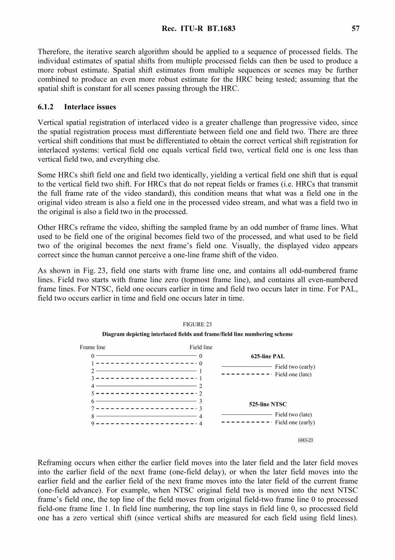
Rec. ITU-R BT.1683 57
Therefore, the iterative search algorithm should be applied to a sequence of processed fields. The individual estimates of spatial shifts from multiple processed fields can then be used to produce a more robust estimate. Spatial shift estimates from multiple sequences or scenes may be further combined to produce an even more robust estimate for the HRC being tested; assuming that the spatial shift is constant for all scenes passing through the HRC.
6.1.2 Interlace issues
Vertical spatial registration of interlaced video is a greater challenge than progressive video, since the spatial registration process must differentiate between field one and field two. There are three vertical shift conditions that must be differentiated to obtain the correct vertical shift registration for interlaced systems: vertical field one equals vertical field two, vertical field one is one less than vertical field two, and everything else.
Some HRCs shift field one and field two identically, yielding a vertical field one shift that is equal to the vertical field two shift. For HRCs that do not repeat fields or frames (i.e. HRCs that transmit the full frame rate of the video standard), this condition means that what was a field one in the original video stream is also a field one in the processed video stream, and what was a field two in the original is also a field two in the processed.
Other HRCs reframe the video, shifting the sampled frame by an odd number of frame lines. What used to be field one of the original becomes field two of the processed, and what used to be field two of the original becomes the next frame’s field one. Visually, the displayed video appears correct since the human cannot perceive a one-line frame shift of the video.
As shown in Fig. 23, field one starts with frame line one, and contains all odd-numbered frame lines. Field two starts with frame line zero (topmost frame line), and contains all even-numbered frame lines. For NTSC, field one occurs earlier in time and field two occurs later in time. For PAL, field two occurs earlier in time and field one occurs later in time.
1683-23
0011223344
0123456789
FIGURE 23Diagram depicting interlaced fields and frame/field line numbering scheme
Frame line Field line625-line PAL
Field two (early)Field one (late)
525-line NTSC
Field two (late)Field one (early)
Reframing occurs when either the earlier field moves into the later field and the later field moves into the earlier field of the next frame (one-field delay), or when the later field moves into the earlier field and the earlier field of the next frame moves into the later field of the current frame (one-field advance). For example, when NTSC original field two is moved into the next NTSC frame’s field one, the top line of the field moves from original field-two frame line 0 to processed field-one frame line 1. In field line numbering, the top line stays in field line 0, so processed field one has a zero vertical shift (since vertical shifts are measured for each field using field lines).

58 Rec. ITU-R BT.1683
When original NTSC field one is moved to that frame’s field two, the top line of the field moves from original field one, frame line 1 to processed field two, frame line 2. In field line numbering, the top line moves from field line 0 to field line 1, so processed field two has a one field line vertical shift. The general rule for both NTSC and PAL is that when the field-two vertical shift (in field lines) is one greater than the field-one vertical shift (in field lines), reframing has occurred.
If the field-two vertical shift is not equal to or one more than the field-one vertical shift, the HRC has corrupted the proper spatial sampling of the two interlaced fields of video and the resulting video will appear to “bob” up and down. Such an impairment is both obvious and annoying to the viewer, and hence seldom occurs in practice since the HRC designer discovers and corrects the error. Therefore, most of the time, spatial registration simplifies into two common patterns. In systems that do not reframe, field-one vertical shift equals field-two vertical shift; and in systems that reframe, field-one vertical shift plus one equals field-two vertical shift.
Additionally, notice that spatial registration includes some temporal registration information, specifically whether the video has been reframed or not. The temporal registration process may or may not be able to detect reframing, but even if it can, reframing is inherent to the spatial registration process. Therefore, spatial registration must be able to determine whether the processed field being examined best aligns with an original field one or field two. The spatial registration for each field can only be correctly computed when the processed field is compared to the original field that created it. Aside from the reframing issue, use of the wrong original field (field one versus field two) can produce spatial registration inaccuracies due to the inherent differences in the spatial content of the two interlaced fields.
6.1.3 Required inputs to the spatial registration algorithm
This section gives a list of the input variables that are required by the spatial registration algorithm. These inputs specify items such as the range of spatial shifts and temporal fields over which to search. If these ranges are overly generous, the speed of convergence of the iterative search algorithm used to find the spatial shift may be slow and the probability of false spatial registration for scenes with repetitive content is increased (e.g. someone waving their hand). Conversely, if these ranges are too restrictive, the search algorithm will encounter, and slowly extend, the search range boundaries with successive iterations. While this built-in search intelligence is useful if the user mis-guesses the search uncertainties by a small amount, the undesirable side effect is to dramatically increase run time when the user mis-guesses by a large amount. Alternatively, the search algorithm may fail to find the correct spatial shift in this case.
6.1.3.1 Expected range of spatial shifts
The expected range of spatial shifts for 525-line and 625-line video sampled according to Recommendation ITU-R BT.601 lies between ±20 pixels horizontally and ±12 field lines vertically. This range of expected shifts has been determined empirically by processing video data from hundreds of HRCs. The expected range of spatial shifts for video sampled according to other formats smaller than Recommendation ITU-R BT.601 (e.g. CIF), is presumed to be half of that observed for 525-line and 625-line systems. This search algorithm should operate correctly, albeit a bit slower, when the processed field has spatial shifts that lie outside of the expected range of spatial shifts. This is because the search algorithm will expand the search beyond the expected range of spatial shifts when warranted. Excursions exceeding 50% of the expected range, however, may report a failure to find the correct spatial registration.
6.1.3.2 Temporal uncertainty
The user must also specify the temporal registration uncertainty, i.e. the range of original fields to examine for each processed field. This temporal uncertainty is expressed as a number of frames before and after the default temporal registration. If the original and processed video sequences are

Rec. ITU-R BT.1683 59
stored as files, then a reasonable default temporal registration is to assume that the first frames in each file align. The temporal uncertainty that is specified should be large enough to include the actual temporal registration. An uncertainty of plus or minus one second (30 frames for 525-line NTSC video; 25 frames for 625-line PAL video) should be sufficient for most video systems. HRCs with long video delays may require a larger temporal uncertainty. The search algorithm may examine temporal registrations outside of the specified uncertainty range when warranted (e.g. when the farthest original field is chosen as the best temporal registration).
6.1.3.3 PVR guess
The PVR guess specifies the portion of the processed image that has not been blanked or corrupted due to processing, presuming no spatial shift has occurred (since the spatial shift has not yet been measured). Although the PVR guess could be determined empirically, a user-specified PVR guess that excludes the over-scan is a good choice. In most cases this will eliminate invalid video from being used in the spatial registration algorithm. For 525-line/NTSC video sampled according to Recommendation ITU-R BT.601, the over-scan covers approximately 18 frame lines at the top and bottom of the frame, and 22 pixels at the left and right sides of the frame. For 625-line/PAL video sampled according to Recommendation ITU-R BT.601, the over-scan covers approximately 14 frame lines at the top and bottom of the frame, and 22 pixels at the left and right sides of the frame. When using other image sizes (e.g. CIF), a reasonable default PVR for these image sizes should be selected.
6.1.4 Sub-algorithms used by the spatial registration algorithm
The spatial registration algorithm makes use of a number of sub-algorithms, including estimation of gain and level offset, and the formula used to determine the closest matching original field for a given processed field. These sub-algorithms have been designed to be computationally efficient, since they must be performed many times by the iterative search algorithm.
6.1.4.1 ROI used by all calculations
All field comparisons made by the algorithm will be between spatially shifted versions of a ROI extracted from the processed video (to compensate for the spatial shifts introduced by the HRC) and the corresponding ROI extracted from the original video. The spatially shifted ROI from the processed video will be denoted as PROI (i.e. processed ROI) and the corresponding ROI from the original video will be denoted as OROI (original ROI). The rectangle coordinates that specify OROI are fixed throughout the algorithm and are chosen to give the largest possible OROI that meets both of the following requirements: – The OROI must correspond to a PROI that lies within the PVR for all possible spatial shifts
that will be examined. – The OROI is centred within the original image.
6.1.4.2 Gain and level offset
The following algorithm is used to estimate the gain of the processed video. The processed field being examined is shift-corrected using the current estimate for spatial shift. After this shift-correction, a PROI is selected that corresponds to the fixed OROI determined in § 6.1.4.1. Next, the standard deviation of the luminance (Y) pixels from this PROI and the standard deviation of the luminance pixels (Y) from the OROI are calculated. Gain is then estimated as the standard deviation of PROI pixels divided by the standard deviation of OROI pixels.
The reliability of this gain estimate improves as the algorithm iterates toward the correct spatial and temporal shift. A gain of 1.0 (i.e. no gain correction) may be used during the first several iteration cycles. The above gain calculation is sensitive to impairments in the processed video such as

60 Rec. ITU-R BT.1683
blurring. However, for the purposes of spatial registration, this gain estimate is appropriate because it makes the processed video look as much like the original video as possible. To remove gain from the processed field, each luminance pixel in the processed field is divided by the gain.
There is no need to determine or correct for level offset, since the spatial registration algorithm’s search criteria are unaffected by level offsets (see § 6.1.4.3).
6.1.4.3 Formulae used to compare PROI with OROI
After correcting the PROI for gain3 (§ 6.1.4.2), the standard deviation of the (OROI-PROI) difference image is used to choose between two or more spatial shifts or temporal shifts. The gain estimate from the previous best match is used to correct the PROI gain. To search among several spatial shifts (with temporal shift held constant), compute the standard deviation of the (OROI-PROI) difference image for several PROI generated using different spatial shifts. For a given processed field, the combination of spatial and temporal shifts that produce the smallest standard deviation (i.e. most cancellation with the original) is chosen as the best match.
6.1.5 Spatial registration using arbitrary scenes
Spatial registration of a processed field from a scene must examine a plurality of original fields and spatial shifts since both the temporal shift (i.e. video delay) and the spatial shift are unknown. As a result, the search algorithm is complex and computationally intense. Furthermore, the scene content is arbitrary, and so the algorithm may find an incorrect spatial registration (see § 6.1.1). Therefore, the prudent course is to compute the spatial registration of several processed fields from several different scenes that have all been passed through the same HRC, and combine the results into one robust estimate of spatial shift. A single HRC should have one constant spatial registration. If not, these time varying spatial shifts would be perceived as an impairment (e.g. the video would bounce up and down or from side to side). This section describes the spatial registration algorithm from the bottom up, in that the core components of the algorithm are described first, and then their application for spatial registering scenes and HRCs is described.
6.1.5.1 Best original field match in time
When spatially registering, using scene content, the algorithm must find the original field that most closely matches the current processed field. Unfortunately, that original field may not actually exist. For example, a processed field may contain part of two different original fields since it may have been interpolated from other processed fields. The current estimate of the best original field match (i.e. that original field that most closely matches the current processed field) is kept at all stages of the search algorithm.
An initial assumption is made that the first field of the processed Big YUV file aligns with the first field of the original Big YUV file, within plus or minus some temporal uncertainty in frames (denoted here as U). For each processed field that is examined by the algorithm, there must be a buffer of U original frames before and after this field. Thus, the algorithm starts examining processed fields that are U frames into the file, and examines every frequencyth frame thereafter (denoted here as F), stopping U frames before the end of the file.
The final search results from the previous processed field (gain, vertical and horizontal shift, temporal shift) are used to initialize the search for the current processed field. The best original field
3 Gain compensation can sometimes be omitted to decrease the computational complexity. However,
omission of gain correction is only recommended during early stages of the iterative search algorithm, where the goal is to find the approximate spatial registration (e.g. see § 6.1.5.2 and 6.1.5.3).
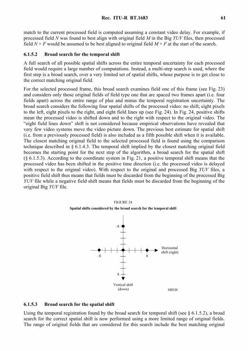
Rec. ITU-R BT.1683 61
match to the current processed field is computed assuming a constant video delay. For example, if processed field N was found to best align with original field M in the Big YUV files, then processed field N + F would be assumed to be best aligned to original field M + F at the start of the search.
6.1.5.2 Broad search for the temporal shift
A full search of all possible spatial shifts across the entire temporal uncertainty for each processed field would require a large number of computations. Instead, a multi-step search is used, where the first step is a broad search, over a very limited set of spatial shifts, whose purpose is to get close to the correct matching original field.
For the selected processed frame, this broad search examines field one of this frame (see Fig. 23) and considers only those original fields of field type one that are spaced two frames apart (i.e. four fields apart) across the entire range of plus and minus the temporal registration uncertainty. The broad search considers the following four spatial shifts of the processed video: no shift, eight pixels to the left, eight pixels to the right, and eight field lines up (see Fig. 24). In Fig. 24, positive shifts mean the processed video is shifted down and to the right with respect to the original video. The “eight field lines down” shift is not considered because empirical observations have revealed that very few video systems move the video picture down. The previous best estimate for spatial shift (i.e. from a previously processed field) is also included as a fifth possible shift when it is available. The closest matching original field to the selected processed field is found using the comparison technique described in § 6.1.4.3. The temporal shift implied by the closest matching original field becomes the starting point for the next step of the algorithm, a broad search for the spatial shift (§ 6.1.5.3). According to the coordinate system in Fig. 21, a positive temporal shift means that the processed video has been shifted in the positive time direction (i.e. the processed video is delayed with respect to the original video). With respect to the original and processed Big YUV files, a positive field shift thus means that fields must be discarded from the beginning of the processed Big YUV file while a negative field shift means that fields must be discarded from the beginning of the original Big YUV file.
1683-24
–8 8
8
–8
Horizontalshift (right)
Vertical shift(down)
FIGURE 24Spatial shifts considered by the broad search for the temporal shift
6.1.5.3 Broad search for the spatial shift
Using the temporal registration found by the broad search for temporal shift (see § 6.1.5.2), a broad search for the correct spatial shift is now performed using a more limited range of original fields. The range of original fields that are considered for this search include the best matching original
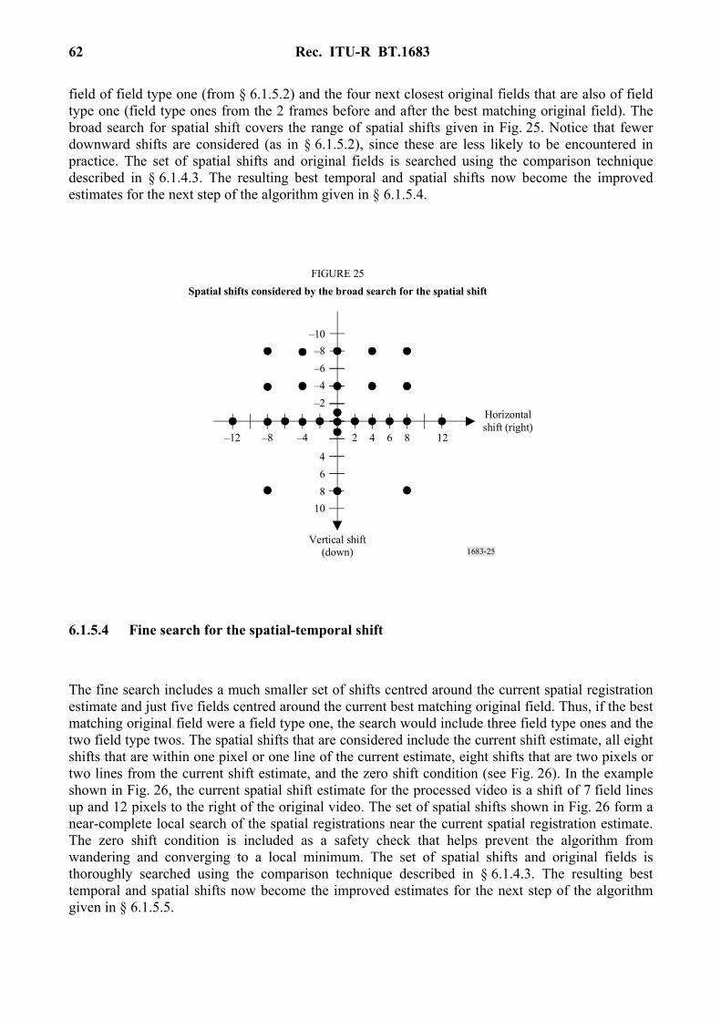
62 Rec. ITU-R BT.1683
field of field type one (from § 6.1.5.2) and the four next closest original fields that are also of field type one (field type ones from the 2 frames before and after the best matching original field). The broad search for spatial shift covers the range of spatial shifts given in Fig. 25. Notice that fewer downward shifts are considered (as in § 6.1.5.2), since these are less likely to be encountered in practice. The set of spatial shifts and original fields is searched using the comparison technique described in § 6.1.4.3. The resulting best temporal and spatial shifts now become the improved estimates for the next step of the algorithm given in § 6.1.5.4.
1683-25
–8 8
8
–4–12 12642
10
64
–2–4–6–8
–10
Horizontalshift (right)
Vertical shift(down)
FIGURE 25Spatial shifts considered by the broad search for the spatial shift
6.1.5.4 Fine search for the spatial-temporal shift
The fine search includes a much smaller set of shifts centred around the current spatial registration estimate and just five fields centred around the current best matching original field. Thus, if the best matching original field were a field type one, the search would include three field type ones and the two field type twos. The spatial shifts that are considered include the current shift estimate, all eight shifts that are within one pixel or one line of the current estimate, eight shifts that are two pixels or two lines from the current shift estimate, and the zero shift condition (see Fig. 26). In the example shown in Fig. 26, the current spatial shift estimate for the processed video is a shift of 7 field lines up and 12 pixels to the right of the original video. The set of spatial shifts shown in Fig. 26 form a near-complete local search of the spatial registrations near the current spatial registration estimate. The zero shift condition is included as a safety check that helps prevent the algorithm from wandering and converging to a local minimum. The set of spatial shifts and original fields is thoroughly searched using the comparison technique described in § 6.1.4.3. The resulting best temporal and spatial shifts now become the improved estimates for the next step of the algorithm given in § 6.1.5.5.

Rec. ITU-R BT.1683 63
1683-26
–7–2 2
–2
2
+12
Relative horizontal
shift
Horizontal shift(left)
Verticalshift(up)
Relative vertical
shift
FIGURE 26Spatial shifts considered by the fine search for the spatial shift
6.1.5.5 Repeated fine searches
Iteration through the fine search of § 6.1.5.4 will move the current estimate for spatial shift a little closer to either the actual spatial shift or (more rarely) a false minimum. Likewise, one iteration through the fine search will move the current estimate for the best-aligned original field either a little closer to the actual best-aligned original field or (more rarely) a little closer to a false minimum. Thus, each fine search will move these estimates closer to a stable value. Because fine searches examine a very limited area spatially and temporally, they must be performed repetitively to assure that convergence has been reached. When gain compensation is being used, the processed field’s gain is estimated anew between each fine search (see § 6.1.4.2).
Repeated fine searches are performed on the processed field (see § 6.1.5.4) until the best spatial shift and the original field associated with that spatial shift remain unchanged from one search to the next. Repeated fine searches are stopped if the algorithm is alternating between two spatial shifts (e.g. a horizontal shift 3 and then a horizontal shift 4, with everything else remaining the same). This alternation is indicated when the current best estimate for spatial shift and the original field associated with that spatial shift, are identical to those found two iterations ago.
Sometimes the repeated search algorithm fails to converge. If the algorithm fails to converge within some requested maximum number of iterations, the iterative search algorithm is terminated and a “failure to find shift” condition is reported for that processed field. This special case does not normally pose a problem because multiple processed fields are examined for each scene (§ 6.1.5.6) and multiple scenes are examined for each HRC (§ 6.1.5.7).
6.1.5.6 Algorithm for one scene
An initial baseline (i.e. starting) estimate for vertical shift, horizontal shift, and temporal registration is computed without any gain compensation as follows. The first temporal uncertainty, U, processed frames in the Big YUV file are skipped. A broad search for the temporal shift is performed on the next processed field of field type one (see § 6.1.5.2). Notice that this broad search will search the first U ⋅ 2 + 1 frames of the original video sequence for a field type one that best aligns. Then, a broad search for the spatial shift is performed centred on this best-aligned original field (see § 6.1.5.3). Next perform up to five fine spatial-temporal searches to fine-tune the spatial and temporal estimates (see § 6.1.5.4 and 6.1.5.5). If these repeated fine searches fail to find a stable
64 Rec. ITU-R BT.1683
result, discard this processed field from consideration. Repeat the above procedure every frequencyth, F, frame until an original field of field type one is found that produces stable results. The baseline estimate will be updated periodically, as described below.
The spatial shift estimates are calculated for both field types of a frame in the processed Big YUV file as follows. Using the baseline estimate as a starting point, perform up to three repeated fine searches on the first processed field of field type one. If the baseline estimate is correct or very nearly correct, the repeated fine searches will yield a stable result. If so, the spatial shift and temporal delay for that processed field are stored in an array that is dedicated to storing the field one results. If a stable result is not found, most likely the spatial shift is correct but the temporal shift estimate is off (i.e. the current estimate of temporal shift is more than two frames away from the true temporal shift). So a broad search for the temporal shift is conducted that includes the current best estimate of spatial shift. This broad search will normally correct the temporal delay estimate. When the broad search for the temporal shift completes, its output is used as the starting point, and up to five repeated fine searches are performed. If this second repeated fine search fails to find a stable result, then report a failed spatial registration for this frame (i.e. both field type one and field type two). If a stable result is found from this second search, then the spatial shift and temporal delay for that field are stored in the field one array. Also, the spatial shift and temporal delay used as the starting point for the next processed field of field type one are updated (i.e. for the first processed field, the baseline results are used and after that, the last stable result is used). After the spatial shift has been estimated for the first processed field of field type one, the spatial shift for the first processed field of field type two is estimated. Using the field one spatial results as the starting point, the same steps are used to find the field-two spatial shift (i.e. the three fine searches, and if needed a broad search for the temporal shift followed by five repeated fine searches). If a stable result is found for field two, store the vertical and horizontal shift for field two in a different array that is dedicated to storing field-two results.
The procedure described in the above paragraph is applied to estimate the spatial shift of both field types of each frequencyth, F, frame in the Big YUV file that contains the processed video. The first temporal uncertainty, U, processed frames in the Big YUV file are skipped. This sequence of estimates is then used to compute robust estimates of the spatial shift for each field type for the scene being examined. The vertical field-one shift results from each frame are sorted, and the 50th percentile retained as the overall vertical field-one shift. Likewise, the vertical field-two shift results from each frame are sorted, and the 50th percentile retained as the overall vertical field-two shift. The horizontal field-one shift results from each frame are sorted, and the 50th percentile retained as the overall horizontal shift. Any difference between field-one and field-two horizontal shift is most likely due to a sub-pixel horizontal shift (e.g. a horizontal shift of 0.5 pixels). Sub-pixel horizontal shifts will produce estimates that include both of the two closest shifts. Using the 50th percentile point allows the most likely horizontal shift to be chosen, which produces a spatial registration accuracy that is good to the nearest 0.5 pixels4.
6.1.5.7 Algorithm for one HRC
If several scenes have been passed through the same HRC, the spatial registration results for each scene should be identical. Thus, filtering results obtained from multiple scenes can increase the robustness and accuracy of the spatial shift measurements. The overall HRC spatial registration results can then be used to compensate all of the processed video for that HRC.
4 Spatial registration to the nearest 0.5 pixels is sufficient for the video quality measurements described in this Annex. Sub-pixel spatial registration techniques are beyond the scope of this Annex.

Rec. ITU-R BT.1683 65
6.1.5.8 Comments on algorithm
Some video scenes are simply not well suited for estimating spatial registration. The described algorithm will sometimes locate a false minimum. Other times, the algorithm will wander between multiple solutions and never reach a stable result. For these reasons, it is advisable to examine multiple images within the same scene and to median filter (i.e. sort results from low to high and select the 50th percentile point) these results across different scenes. The spatial registration by scenes algorithm is an heuristic algorithm that utilizes patterns of spatial shifts that have been observed from a sampling of video systems. These assumptions may be incorrect for some systems, causing the algorithm to find an incorrect spatial shift. However, failure of the algorithm tends to produce spatial shifts that are inconsistent from frame to frame and from scene to scene (i.e. when the algorithm fails, it normally produces a scattering of results). When the algorithm outputs the same or very similar spatial shifts for each scene, a high degree of confidence is indicated. When the individual field results for a scene wander, a low degree of confidence is indicated.
6.1.6 Spatial registration of progressive video
Spatial registration of progressive video follows the same steps as the interlace algorithms, with minor modifications. Where the interlace algorithms operate on field one and field two separately, the progressive algorithm operates on frames. Thus, all mentions of field two are ignored and, with the exception of the fine searches, the range of vertical shifts is doubled.
The modification of the vertical shift range is most important for the broad spatial shift. When doing a broad search for spatial shift (see § 6.1.5.3) the numbers on the vertical axis in Fig. 25 must be doubled (e.g. +8 becoming +16 and –4 becoming –8)5. In addition, for progressive CIF and QCIF images, the horizontal and vertical broad spatial search ranges are halved due to the smaller shifts that are typically encountered with these image sizes. For example, using CIF images in Fig. 25, the horizontal axis would stretch from –6 to +6 pixels and the vertical axis would stretch from –8 to +8 frame lines.
The temporal search range, being stated in frames, is largely unchanged. For the broad temporal search in § 6.1.5.2, instead of matching one processed field one to every second original field one, the progressive algorithm compares one processed frame to every second original frame. For the colourbar algorithm, the search examines spatial shifts for one processed frame and one original frame (i.e. no temporal searching).
The only step requiring more complicated changes is the fine search from § 6.1.5.4. Here, the vertical shifts remain unchanged, lying between –2 frame lines and +2 frame lines. Thus, the vertical axis of Fig. 26 is interpreted as referring to frame lines. The temporal extent of this fine search may be set to five original frames centred on the current aligned original frame, instead of the three original frames otherwise implied. A five-frame search extent may improve the speed and efficiency of the fine search when compared to the interlace version of the algorithm, since progressive HRCs are more likely to contain varying video delay than non-zero spatial shifts.
When considering the algorithmic changes for progressive video systems, many of the spatial shift search parameters can be modified without harming the integrity of the algorithm. As an example, consider spatial shifts other than zero pixels and zero lines for the broad temporal search. The spatial shift at zero pixels horizontally and 8 field lines vertically for interlace video could be moved to 16 frame lines for progressive video, as recommended above, or placed at 8 frame lines,
5 In one possible exception to this doubling, the spatial shift associated with zero pixels horizontally and
plus or minus one field line vertically could be left at plus or minus one frame line vertically. Spatial shifts very close to (zero, zero) are commonly encountered.
66 Rec. ITU-R BT.1683
under the assumption that progressive video sequences are unlikely to contain 16 frame lines of vertical shift. Likewise, spatial shift at zero lines vertically and 8 pixels horizontally could be moved to 9 or 10 pixels horizontally without any detrimental effects. As another example, the exact number of repeated fine searches performed could be increased or decreased for specific applications. The exact values recommended here are significantly less important than the actual structure of the search algorithm.
6.2 Valid region
NTSC (525-line) and PAL (625-line) video sampled according to Recommendation ITU-R BT.601 may have a border of pixels and lines that do not contain a valid picture. The original video from the camera may only fill a portion of the Recommendation ITU-R BT.601 frame. A digital video system that utilizes compression may further reduce the area of the picture in order to save transmission bits. If the non-transmitted pixels and lines occur in the over-scan area of the television picture, the typical end-user should not notice the missing lines and pixels. If these non-transmitted pixels and lines exceed the over-scan area, the viewer may notice a black border around the picture, since the system will normally insert black into this non-transmitted picture area. Video systems (particularly those that perform low-pass filtering) may exhibit a ramping up from the black border to the picture area. These transitional effects most often occur at the left and right sides of the image but can also occur at the top or bottom. Occasionally, the processed video may also contain several lines of corrupted video at the top or bottom of the picture that may not be visible to the viewer (e.g. VHS tape recorders corrupt several lines at the bottom of the picture in the over-scan area). To prevent non-picture areas from influencing the VQM measurements, these areas should be excluded from the VQM measurement. The automated valid region algorithm presented here estimates the valid region of the original and processed video streams so that subsequent computations do not consider corrupted lines at the top and bottom of the Recommendation ITU-R BT.601 frame, black border pixels, or transitional effects where the black border meets the picture area.
6.2.1 Core valid region algorithm This section describes the core valid region algorithm that is applied to a single original or processed image. This algorithm requires three input arguments: an image, a maximum valid region, and the current valid region estimate. – Image: the core algorithm uses the Recommendation ITU-R BT.601 luminance image of a
single video frame. When measuring the valid region of a processed video sequence, any spatial shift imposed by the video system must have been removed from the luminance image before applying the core algorithm (see § 6.1).
– Maximum valid region: the core algorithm will not consider pixels and lines outside of a maximum valid video region. This provides a mechanism for the user to specify a maximum valid region that is smaller than the entire image area if a priori knowledge indicates that the sampled image has corrupted pixels or lines as discussed in § 6.2.
– Current valid region: the current valid region is an estimate of the valid region and lies entirely within the maximum valid region. All pixels inside the current valid region are known to contain valid video; pixels outside the current valid region may or may not contain valid video content. Initially, the current valid region is set to the smallest possible area located at the exact centre of the image.
The core algorithm examines the area of video between the maximum valid region and the current valid region. If some of those pixels appear to contain valid video, the current valid region estimate is enlarged. The algorithm will now be described in detail for the left edge of the image.
Step 1: Compute the mean of the left-most column of pixels in the maximum valid region. The left-most column of pixels will be denoted as column J-1 and the mean will be represented by MJ-1.

Rec. ITU-R BT.1683 67
Step 2: Take the mean of the next column of pixels, MJ.
Step 3: Column J is declared invalid video if it is black, (MJ < 20) or if the average pixel level of the mean value for successive columns indicates a ramp up from black border to valid picture (MJ – 2 > MJ-1). If either of these conditions are true, increment J and repeat Steps 2 and 3. Otherwise, go to Step 4.
Step 4: If final column J is within the current valid region, then no new information has been obtained. Otherwise, update the current valid region with J as the left coordinate.
The algorithm for finding the top edge of the image is similar to that given above for the left edge. For the bottom and right edges, J is decremented instead of incremented; otherwise the algorithm is the same. The values produced for top, left, bottom, and right indicate the last valid pixel or line.
The stopping conditions identified in Step 3 can be fooled by scene content. For example, an image that contains genuine black at the left side (i.e. black that is part of the scene) will cause the core algorithm to conclude that the left-most valid column of video is farther toward the middle of the image than it ought to be. For that reason, the core algorithm is applied to multiple images from a video sequence, thereby increasing the accuracy of the valid region estimate.
6.2.2 Applying the core valid region algorithm to a video sequence
6.2.2.1 Original video
The core algorithm is first applied to the original sequence of images. For NTSC video sampled according to Recommendation ITU-R BT.601 (see § 5), the recommended setting for the maximum valid region is top = 6, left = 6, bottom = 482, right = 714. For PAL video sampled according to Recommendation ITU-R BT.601, the recommended setting for the maximum valid region is top = 6, left = 16, bottom = 570, right = 704. The core algorithm is run on the first image in the video sequence, and every frequencyth image thereafter. For example, if the specified frequency were 15, the core algorithm would examine sequence image numbers 0, 15, 30, 45, and so forth. When all images in the sequence have been examined, the current valid region will contain the largest valid area implied by any examined image in the video sequence. Pixels and lines between this final current valid region and the maximum valid region are considered to contain either black or a transitional ramp up from black.
The final valid region must contain an even number of lines and an even number of pixels. Any odd top or left coordinates are incremented by one. Then, if the region contains an odd number of lines, bottom is decremented; likewise, if the region contains an odd number of pixels (e.g. horizontally), right is decremented. This simplifies colour processing for video sampled in accordance with Recommendation ITU-R BT.601, since the colour channels are sub-sampled by 2 when compared to the luminance channel. Also, each interlaced field of video will contain the same number of video lines. This will assure that spatial-temporal sub-regions (from which features will be extracted) always contain valid video with equal contributions from both interlaced fields. The resulting valid region is returned as the original valid region.
6.2.2.2 Processed video
When computing the valid region of the processed video sequence, the maximum valid region setting for the core algorithm is first set equal to the corresponding original valid region found for that scene. This maximum valid region is then reduced in size by any pixels and lines that are considered invalid due to spatially shift correcting the processed video frames. The core algorithm is then run on the first image in the processed video sequence, and every frequencyth image thereafter (i.e. if frequency = F, use images Y(0), Y(F), Y(2F), Y(3F), and so forth).
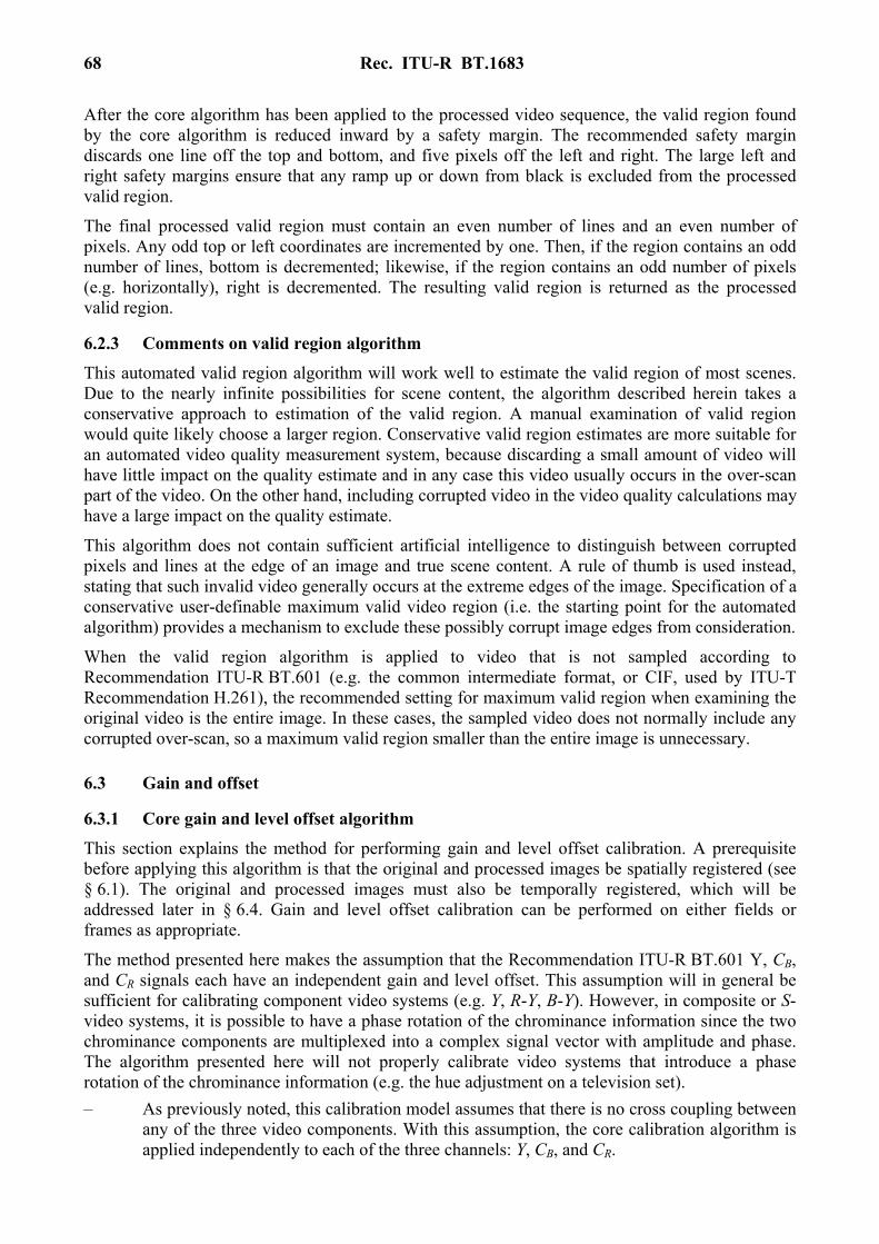
68 Rec. ITU-R BT.1683
After the core algorithm has been applied to the processed video sequence, the valid region found by the core algorithm is reduced inward by a safety margin. The recommended safety margin discards one line off the top and bottom, and five pixels off the left and right. The large left and right safety margins ensure that any ramp up or down from black is excluded from the processed valid region.
The final processed valid region must contain an even number of lines and an even number of pixels. Any odd top or left coordinates are incremented by one. Then, if the region contains an odd number of lines, bottom is decremented; likewise, if the region contains an odd number of pixels (e.g. horizontally), right is decremented. The resulting valid region is returned as the processed valid region.
6.2.3 Comments on valid region algorithm This automated valid region algorithm will work well to estimate the valid region of most scenes. Due to the nearly infinite possibilities for scene content, the algorithm described herein takes a conservative approach to estimation of the valid region. A manual examination of valid region would quite likely choose a larger region. Conservative valid region estimates are more suitable for an automated video quality measurement system, because discarding a small amount of video will have little impact on the quality estimate and in any case this video usually occurs in the over-scan part of the video. On the other hand, including corrupted video in the video quality calculations may have a large impact on the quality estimate.
This algorithm does not contain sufficient artificial intelligence to distinguish between corrupted pixels and lines at the edge of an image and true scene content. A rule of thumb is used instead, stating that such invalid video generally occurs at the extreme edges of the image. Specification of a conservative user-definable maximum valid video region (i.e. the starting point for the automated algorithm) provides a mechanism to exclude these possibly corrupt image edges from consideration.
When the valid region algorithm is applied to video that is not sampled according to Recommendation ITU-R BT.601 (e.g. the common intermediate format, or CIF, used by ITU-T Recommendation H.261), the recommended setting for maximum valid region when examining the original video is the entire image. In these cases, the sampled video does not normally include any corrupted over-scan, so a maximum valid region smaller than the entire image is unnecessary.
6.3 Gain and offset
6.3.1 Core gain and level offset algorithm This section explains the method for performing gain and level offset calibration. A prerequisite before applying this algorithm is that the original and processed images be spatially registered (see § 6.1). The original and processed images must also be temporally registered, which will be addressed later in § 6.4. Gain and level offset calibration can be performed on either fields or frames as appropriate.
The method presented here makes the assumption that the Recommendation ITU-R BT.601 Y, CB, and CR signals each have an independent gain and level offset. This assumption will in general be sufficient for calibrating component video systems (e.g. Y, R-Y, B-Y). However, in composite or S-video systems, it is possible to have a phase rotation of the chrominance information since the two chrominance components are multiplexed into a complex signal vector with amplitude and phase. The algorithm presented here will not properly calibrate video systems that introduce a phase rotation of the chrominance information (e.g. the hue adjustment on a television set). – As previously noted, this calibration model assumes that there is no cross coupling between
any of the three video components. With this assumption, the core calibration algorithm is applied independently to each of the three channels: Y, CB, and CR.
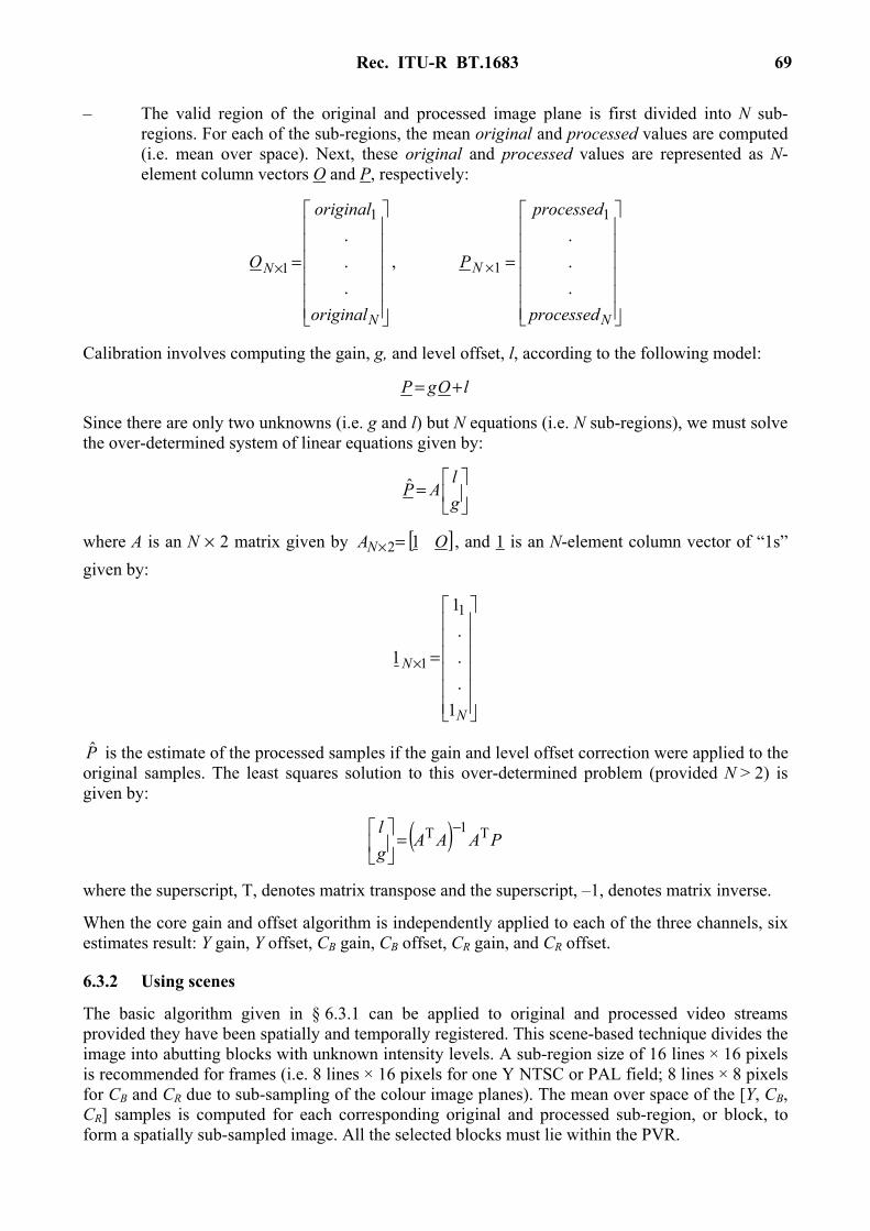
Rec. ITU-R BT.1683 69
– The valid region of the original and processed image plane is first divided into N sub-regions. For each of the sub-regions, the mean original and processed values are computed (i.e. mean over space). Next, these original and processed values are represented as N-element column vectors O and P, respectively:
=×
N
N
original
original
O...
1
1 ,
=×
N
N
processed
processed
P...
1
1
Calibration involves computing the gain, g, and level offset, l, according to the following model:
lOgP +=
Since there are only two unknowns (i.e. g and l) but N equations (i.e. N sub-regions), we must solve the over-determined system of linear equations given by:
=
gl
AP
where A is an N × 2 matrix given by [ ]OAN 12=× , and 1 is an N-element column vector of “1s” given by:
=×
N
N
1...
1
1
1
1
P is the estimate of the processed samples if the gain and level offset correction were applied to the original samples. The least squares solution to this over-determined problem (provided N > 2) is given by:
( ) PAAAgl T1T −
=
where the superscript, T, denotes matrix transpose and the superscript, –1, denotes matrix inverse.
When the core gain and offset algorithm is independently applied to each of the three channels, six estimates result: Y gain, Y offset, CB gain, CB offset, CR gain, and CR offset.
6.3.2 Using scenes
The basic algorithm given in § 6.3.1 can be applied to original and processed video streams provided they have been spatially and temporally registered. This scene-based technique divides the image into abutting blocks with unknown intensity levels. A sub-region size of 16 lines × 16 pixels is recommended for frames (i.e. 8 lines × 16 pixels for one Y NTSC or PAL field; 8 lines × 8 pixels for CB and CR due to sub-sampling of the colour image planes). The mean over space of the [Y, CB, CR] samples is computed for each corresponding original and processed sub-region, or block, to form a spatially sub-sampled image. All the selected blocks must lie within the PVR.

70 Rec. ITU-R BT.1683
6.3.2.1 Registering the processed images
For simplicity, we will assume that the best spatial registration has already been found using one of the techniques presented in § 6.1. Before gain and level offset are estimated, each processed image must also be temporally registered. The original image that best aligns with the processed image must be used for the gain and level offset calculation. If the video delay is variable, this temporal registration must be performed for each processed image. If the video delay is constant for the scene, the temporal registration only needs to be performed once.
To temporally register a processed image, first create the spatially sub-sampled original and processed fields (or frames for progressive video) as specified in § 6.3.2, after correcting for the spatial shift of the processed video. Using the sub-sampled Y images, apply the search function given in § 6.1.4.3, except one performs this search using all the original images that are within the temporal registration uncertainty, U. Use the best resulting temporal registration for all three image planes, Y, CB, and CR.
6.3.2.2 Gain and level offset of registered images
An iterative least squares solution with a cost function is used to help minimize the weight of outliers in the fit. This is because outliers are normally due to distortions rather than pure level offset and gain changes, and assigning equal weight to these outliers would distort the fit.
The following algorithm is applied separately to the N matching original and processed pixels from each of the three spatially sub-sampled images [Y, CB, CR].
Step 1: Use the normal least squares solution from § 6.3.1 to generate the initial estimate of the
level offset and gain: ( ) PAAAgl T1T −
=
.
Step 2: Generate an error vector, E, that is equal to the absolute value of the difference between the true processed samples and the fitted processed samples: PPE ˆ−= .
Step 3: Generate a cost vector, C, that is the element-by-element reciprocal of the error vector, E, plus a small epsilon, ε:
ε+=
EC 1 . The ε prevents division by zero and sets the relative weight of a
point that is on the fitted line versus the weight of a point that is off the fitted line. An ε of 0.1 is recommended.
Step 4: Normalize the cost vector C for unity norm (i.e. each element of C is divided by the square root of the sum of the squares of all the elements of C).
Step 5: Generate the cost vector C 2 that is the element-by-element square of the cost vector C from Step 4.
Step 6: Generate an N × N diagonal cost matrix, C 2, that contains the cost vector’s elements, C 2, arranged on the diagonal, with zeros everywhere else.
Step 7: Using the diagonal cost matrix, C 2, from Step 6, perform cost-weighted least squares
fitting to determine the next estimate of the level offset and gain: ( ) PCAACAgl 2T12T −
=
.
Step 8: Repeat Steps 2 through 7 until the level offset and gain estimates converge to four decimal places.

Rec. ITU-R BT.1683 71
These steps are applied separately to processed field one and processed field two, to obtain two estimates for g and l. Field one and two must be examined separately, because the temporally registered original fields need not correspond to one frame within the original video sequence. For progressive video, the above steps are applied to the entire processed frame at once.
6.3.2.3 Estimating gain and level offset for a video sequence and HRC
The algorithm described above is applied to multiple matching original and processed field pairs distributed every frequencyth frame throughout the scene (for progressive video, original and processed frame pairs). A median filter is then applied to the six time histories of the level offsets and gains to produce average estimates for the scene.
If several scenes have been passed through the same HRC, the level offset and gain for each scene will be considered to be identical. Thus, filtering results obtained from multiple scenes can increase the robustness and accuracy of the level offset and gain measurements. The overall HRC level offset and gain results can then be used to compensate all of the processed video for that HRC.
6.3.3 Applying gain and level offset corrections
The temporal registration algorithms (see § 6.4) and most quality features (§ 7) will specify that the gain calculated herein should be removed. To remove gain and level offset from the Y plane, apply the following formula to each processed pixel:
gtjiYtjiY /]1),,([),,(New −=
Gain and level offset correction is not performed on the colour planes (i.e. CB and CR). Perceptual chrominance errors are instead captured by the colour metrics. The CB and CR image planes may be gain and level offset corrected for display purposes.
6.4 Temporal registration
Modern digital video communication systems typically require several tenths of a second to process and transmit the video from the sending camera onto the receiving display. Excessive video delays impede effective two-way communication. Therefore, objective methods for measuring end-to-end video communications delay are important to end-users for specification and comparison of services and to equipment/service providers to optimize and maintain their product offerings. Video delay can depend upon dynamic attributes of the original scene (e.g. spatial detail, motion) and video system (e.g. bit-rate). For instance, scenes with large amounts of motion can suffer more video delay than scenes with small amounts of motion. Thus, video delay measurements should be made in-service to be truly representative and accurate. Estimates of video delay are required to temporally align the original and processed video features shown in Fig. 19 before making quality measurements.
Some video transmission systems may provide time synchronization information (e.g. original and processed frames may be labelled with some kind of a frame numbering scheme). In general, however, time synchronization between the original and processed video streams must be measured. This section presents a technique for estimating video delay based upon the original and processed video frames. The technique is “frame-based” in that it works by correlating lower resolution images, sub-sampled in space and extracted from the original and processed video streams. This frame-based technique estimates the delay of each frame or field (for interlaced video systems). These individual estimates are combined to estimate the average delay of the video sequence.

72 Rec. ITU-R BT.1683
6.4.1 Frame-based algorithm for estimating variable temporal delays between original and processed video sequences
This section describes a frame-based temporal registration algorithm. To reduce the influence of distortions on temporal registration, images are spatially sub-sampled and normalized to have unit variance. This algorithm temporally registers each processed image separately, locating the most similar original image. Some of these individual temporal registration measurements may be incorrect but those errors will tend to be randomly distributed. When delay measurements from a series of images are combined by means of a voting scheme, the overall estimate for the average delay of a video sequence becomes quite accurate. This temporal registration algorithm does not use still and nearly motionless portions of the scene, since the original images are nearly identical to each other.
6.4.1.1 Constants used by the algorithm BELOW_WARN: Threshold used when examining correlations for deciding if a secondary
correlation maximum is sufficiently large so as to indicate ambiguous temporal registration. A BELOW_WARN of 0.9 is recommended.
BLOCK_SIZE: The sub-sampling factor. Specified in frame lines vertically and pixels horizontally. A BLOCK_SIZE of 16 is recommended.
DELTA: Secondary maximums in the correlation curve that are within DELTA of the maximum (best) correlation are ignored. A DELTA of 4 is recommended.
HFW: Half of the filter width for the filter used to smooth the histogram of frame-by-frame temporal registration values. A HFW of 3 is recommended.
STILL_THRESHOLD: A threshold that is used to detect still video scenes (frame-based temporal registration cannot be used on still video scenes). A STILL_THRESHOLD of 0.002 is recommended.
6.4.1.2 Inputs to the algorithm
A sequence of N original video luminance images: YO(t), 0 ≤ t < N 6.
A sequence of N processed video luminance images: YP(t), 0 ≤ t < N.
Gain and offset correction factors for the processed luminance images.
Spatial registration information: horizontal shift and vertical shift. For interlace video, the vertical shift for each field determines whether the processed video requires reframing.
Valid region of the processed video sequence (i.e. PVR).
Uncertainty (U): a number indicating the accuracy of the initial temporal registration. The initial temporal registration assumption is that the true temporal registration for YP(t) is within plus or minus (U – HFW) of YO(t), for all 0 ≤ t < N.
6.4.1.3 Frames versus fields The frame-based temporal registration algorithm works for both progressive and interlace video. If the video sequence is progressive, the algorithm aligns frames. If the video sequence is interlaced, the algorithm aligns fields. When aligning interlaced video sequences, either frame or reframed
6 When interlace video requires reframing, the lengths of the original and processed video sequences must
be reduced by one to accommodate the reframing. This will reduce the length of the file by one video frame from N as specified in Fig. 20.
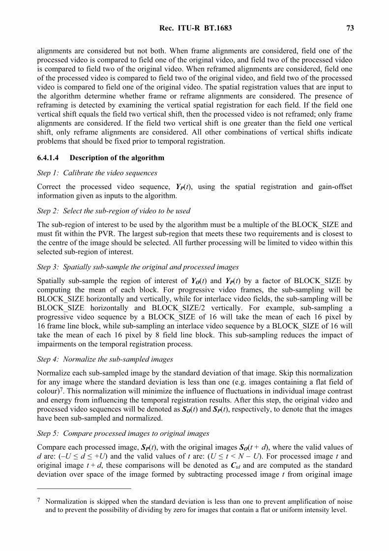
Rec. ITU-R BT.1683 73
alignments are considered but not both. When frame alignments are considered, field one of the processed video is compared to field one of the original video, and field two of the processed video is compared to field two of the original video. When reframed alignments are considered, field one of the processed video is compared to field two of the original video, and field two of the processed video is compared to field one of the original video. The spatial registration values that are input to the algorithm determine whether frame or reframe alignments are considered. The presence of reframing is detected by examining the vertical spatial registration for each field. If the field one vertical shift equals the field two vertical shift, then the processed video is not reframed; only frame alignments are considered. If the field two vertical shift is one greater than the field one vertical shift, only reframe alignments are considered. All other combinations of vertical shifts indicate problems that should be fixed prior to temporal registration.
6.4.1.4 Description of the algorithm
Step 1: Calibrate the video sequences
Correct the processed video sequence, YP(t), using the spatial registration and gain-offset information given as inputs to the algorithm.
Step 2: Select the sub-region of video to be used
The sub-region of interest to be used by the algorithm must be a multiple of the BLOCK_SIZE and must fit within the PVR. The largest sub-region that meets these two requirements and is closest to the centre of the image should be selected. All further processing will be limited to video within this selected sub-region of interest.
Step 3: Spatially sub-sample the original and processed images
Spatially sub-sample the region of interest of YO(t) and YP(t) by a factor of BLOCK_SIZE by computing the mean of each block. For progressive video frames, the sub-sampling will be BLOCK_SIZE horizontally and vertically, while for interlace video fields, the sub-sampling will be BLOCK_SIZE horizontally and BLOCK_SIZE/2 vertically. For example, sub-sampling a progressive video sequence by a BLOCK_SIZE of 16 will take the mean of each 16 pixel by 16 frame line block, while sub-sampling an interlace video sequence by a BLOCK_SIZE of 16 will take the mean of each 16 pixel by 8 field line block. This sub-sampling reduces the impact of impairments on the temporal registration process.
Step 4: Normalize the sub-sampled images
Normalize each sub-sampled image by the standard deviation of that image. Skip this normalization for any image where the standard deviation is less than one (e.g. images containing a flat field of colour)7. This normalization will minimize the influence of fluctuations in individual image contrast and energy from influencing the temporal registration results. After this step, the original video and processed video sequences will be denoted as SO(t) and SP(t), respectively, to denote that the images have been sub-sampled and normalized.
Step 5: Compare processed images to original images
Compare each processed image, SP(t), with the original images SO(t + d), where the valid values of d are: (–U ≤ d ≤ +U) and the valid values of t are: (U ≤ t < N – U). For processed image t and original image t + d, these comparisons will be denoted as Ctd and are computed as the standard deviation over space of the image formed by subtracting processed image t from original image
7 Normalization is skipped when the standard deviation is less than one to prevent amplification of noise
and to prevent the possibility of dividing by zero for images that contain a flat or uniform intensity level.

74 Rec. ITU-R BT.1683
t + d: Ctd = stdspace(SO(t + d) – SP(t)). These comparisons, Ctd, correlate the t-th processed image with each original image that is within the registration uncertainty. Lower values of Ctd indicate that the processed image looks more like the original image since more of the image variance is cancelled. The range for t, U ≤ t < N – U, covers all processed images for which original images are available for the entire range of temporal registration uncertainty.
Step 6: Perform an overall check for still video
To determine if there is sufficient motion in the video sequence, average Ctd over time index t for each d:
∑−−
=⋅
−=
1
*21 UN
Uttdd C
UNA (100)
This summation (100) includes the range of processed video images t for which the full uncertainty of original images is available. Ad contains one value for each temporal registration delay d being considered. If (maximum(Ad) – minimum(Ad) < STILL_THRESHOLD), then the scene contains insufficient motion for frame-based temporal registration. The entire scene is still or nearly still. The correlation results from the different video delays are then so similar that any differentiation will be due to random chance rather than reliable measurements. If a still video sequence is detected, the user is given a warning to that effect and the algorithm exits at this point.
Step 7: Temporally register each processed image
For each processed image t (U ≤ t < N – U), find the d within the temporal uncertainty (−U ≤ d ≤ +U) that minimizes Ctd. In other words, for each processed image t, find dmin(t) such that Ct dmin(t) ≤ Ctd, for all d. The best temporal registration of processed image t is given by dmin(t). Most of the time, the temporal registration indicated for individual images will be correct or very close to correct. The temporal registration will be incorrect for some images due to various reasons (image distortion, errors, noise, insufficient motion, etc.).
Step 8: Perform a stillness check on each processed image
If for a given processed image t and all values of d (–U ≤ d ≤ U), maximum(Ctd) – minimum(Ctd) < STILL_THRESHOLD, then dmin(t) is undefined for this processed image t. Specifically, there is insufficient motion around image t for frame-based temporal registration to work properly.
Step 9: Form a histogram of all defined temporal registrations
Compute a histogram using all the defined values of dmin(t) with 2*U + 1 bins where each bin represents a different video delay (i.e. from –U to +U). Values of dmin(t) that are undefined (e.g. still images) are left out of the histogram calculation. This histogram, denoted by Hd, is the histogram of temporal delays for all the processed images that had sufficient motion to perform valid temporal registration. Each bin in the histogram contains the number of processed images with that video delay d, where d can take values from –U to +U.
Step 10: Form a smoothed histogram
Histogram Hd is smoothed by convolving it with a low pass filter of length 2*HFW + 1 and defined at index k as:
[ ]
[ ] HFW*20for
)HFW1/()HFW(*cos*5.05.0
)HFW1/()HFW(*cos*5.05.0HFW*2
0
≤≤
+−π+
+−π+=
∑=
ki
kF
i
k (101)

Rec. ITU-R BT.1683 75
When considering the smoothed histogram (101) SHd that results from this step, the HFW bins on each end of SHd are treated as undefined. This restricts the video delays that can be estimated to plus or minus (UNCERTAINTY-HFW). Smoothing of the histogram increases the robustness of the video delay estimates.
Step 11: Examine the histogram information From the original histogram, Hd, and the smoothed histogram, SHd, the following three values are determined: max_H_value: The maximum value of Hd. max_SH_offset: The offset d that maximizes SHd. max_SH_value: The maximum value of SHd (e.g. at d = max_SH_offset).
Next, the following two checks are performed: – Was U large enough? Recall that the first and last HFW bins of Hd are missing from SHd.
Examine the values of Hd in these bins. If (Hd > max_H_value * BELOW_WARN), then the temporal registration uncertainty is too small. The algorithm must be re-run with a larger U. The values of d to check are (–U ≤ d < –U + HFW) and (U – HFW < d ≤ U).
– Does SHd have one well-defined delay? Examine SHd, except within DELTA of max_SH_offset. If (SHd > max_SH_value * BELOW_WARN) for any video delay d where (–U ≤ d < max_SH_offset – DELTA) or (max_SH_offset + DELTA < d ≤ U), then temporal registration is ambiguous.
If the above two checks pass, then the video delay given by max_SH_offset is chosen as the best average temporal registration for the scene.
6.4.1.5 Observations and conclusions The frame-based video delay measurement algorithm uses sub-sampled original and processed video sequences. This algorithm is suitable for aligning video in a fully automated out-of-service environment, prior to performing video quality measurements. The frame-based video delay measurement algorithm estimates the temporal registration for each image, forms histograms of those individual estimates, and then uses the most commonly indicated delay as the overall video delay, or temporal registration, for the selected sequence of video frames.
The delay indicated at the final stage of the algorithm (Step 11 of § 6.4.1.4) may be different from the delay a viewer might choose, if aligning the scenes by eye. Viewers tend to focus on motion, aligning the high motion parts of the scene, where the frame-based algorithm chooses the most often observed delay over all of the frames that were examined. These overall delay histograms can be examined to determine the extent and statistics of any variable video delay present in the HRC.
6.4.2 Applying temporal registration correction All of the quality features will require that the temporal delay calculated herein be removed. For positive delays, remove frames from the beginning of the processed file and the end of the original file. For negative delays, remove frames from the end of the processed file and the beginning of the original file. When reframing interlaced video sequences, the processed sequence is reframed. Thus one field should be removed from the beginning and end of the processed video sequence in addition to the above. Simultaneously, one frame must be removed from either the beginning of the original video file (i.e. –1 field delay overall) or the end of the original video file (i.e. +1 field delay overall).
Correcting for temporal registration will, in effect, shorten the length of available images in the video sequence. For simplicity, all further calculations will be based on the number of video frames available after all calibration corrections have been applied.

76 Rec. ITU-R BT.1683
7 Quality features
7.1 Introduction
A quality feature is defined as a quantity of information associated with, or extracted from, a spatial-temporal sub-region of a video stream (either original or processed). The feature streams that are produced are a function of space and time. By comparing features extracted from the calibrated processed video with features extracted from the original video, a set of quality parameters (§ 8) can be computed that are indicative of perceptual changes in video quality. This section describes a set of quality features that characterize perceptual changes in the spatial, temporal, and chrominance properties of video streams. Normally, a perceptual filter is applied to the video stream to enhance some property of perceived video quality, such as edge information. After this perceptual filtering, features are extracted from spatial-temporal (S-T) sub-regions using a mathematical function (e.g. standard deviation). Finally, a perceptibility threshold is applied to the extracted features.
For the following discussion, an original feature stream will be denoted as fo(s, t) and the corresponding processed feature stream will be denoted as fp(s, t), where s and t are indices that denote the spatial and temporal positions, respectively, of the S-T region within the calibrated original and processed video streams. The features will be assigned lettered subscripts as they are discussed in the following sections, where the subscripted letters are chosen to be indicative of what the feature is measuring. All features operate on frames within a calibrated video sequence (see § 6); any interlace issues are addressed during calibration. All features operate independently of image size (i.e. S-T region size does not change when the image size changes)8.
In summary, feature calculations perform the following steps. Some features may not require those steps marked [Optional].
Step 1: [Optional] Apply a perceptual filter.
Step 2: Divide the video stream into S-T regions.
Step 3: Extract features, or summary statistics, from each S-T region (e.g. mean, standard deviation).
Step 4: [Optional] Apply a perceptibility threshold.
Some features may utilize two or more different perceptual filters.
7.1.1 S-T regions
In general, features are extracted from localized S-T regions after the original and processed video streams have been perceptually filtered. The S-T regions are positioned to divide the video streams into abutting S-T regions. Since the processed video has been calibrated, for each processed video S-T region there exists an original S-T region spanning the identical spatial and temporal position within the video stream. Features are extracted from each S-T region by calculating summary statistics or some other mathematical function over the S-T region of interest.
Each S-T region describes a block of pixels. S-T region sizes are described by: – the number of pixels horizontally, – the number of frame lines vertically, and
8 There is an implicit assumption that the viewing distance as a function of picture height remains fixed
(e.g. closer viewing distances are used for smaller images). See Section 9 for further comments regarding the assumed viewing distance.

Rec. ITU-R BT.1683 77
– the time duration of the region, given in units of equivalent video frames referenced to a 30 fps video system9.
Figure 27 illustrates a S-T region of 8 horizontal pixels × 8 vertical lines × 6 NTSC video frames, for a total of 384 pixels. When applied to 25 fps video (PAL), this same S-T region spans 8 horizontal pixels × 8 vertical lines × 5 video frames, for a total of 320 pixels.
One fifth of a second is a desirable temporal extent, due to the ease of frame rate conversions (i.e. one fifth of a second results in an integer number of video frames for video systems operating at 10 fps, 15 fps, 25 fps and 30 fps). The general rule for frame rate conversion is to take the length of the S-T region in 30 fps video frames, divide by 30 and multiply by the frame rate of the video system under test. S-T regions that contain one video frame are presumed to always contain one video frame, independent of the frame rate.
The spatial region of interest (SROI, see § 3) encompassed by all S-T regions is identical for the original and calibrated processed video sequences. The SROI must lie entirely within the PVR, possibly with a buffer of pixels as required by any convolutional perceptual filter. The horizontal width of the SROI must be evenly divisible by the S-T region’s horizontal extent. Likewise, the vertical height of the SROI must be evenly divisible by the S-T region’s vertical extent. A user might further constrain the SROI to encompass a region of particular interest, such as the centre of the video frame.
Temporally, the original and calibrated processed video sequences are divided into an identical number of S-T regions, beginning with the first frame of temporally aligned video. If the number of valid frames available cannot be evenly divided by the S-T region’s temporal extent, frames at the end of the clip are dropped from consideration.
For some features such as those presented in § 7.2, the 8 × 8_6F block achieves close to maximum correlation with subjective ratings. It should be noted, however, that the correlation decreases slowly as one moves away from the optimum S-T region size. Horizontal and vertical widths up to 32 or even larger and temporal widths up to 30 frames can be used with satisfactory results, giving the objective measurement system designer considerable flexibility in adapting the features to the available storage or transmission bandwidth [Wolf and Pinson, 2001].
After the video stream has been divided into S-T regions, the temporal axis of the feature (t) no longer corresponds to individual frames. Rather, the temporal axis contains a number of samples equal to the number of valid frames in the calibrated video sequence divided by the temporal extent of the S-T region.
When computing two or more features simultaneously, further considerations become important. Ideally, all features should be calculated for the same SROI.
9 All time durations in this Annex will be referenced to the equivalent number of video frames from a 30 fps video system. Thus, time durations of 6 frames (F) is used to represent both 6 frames from an NTSC system (6/30) and 5 frames from a PAL system (5/25). In addition, 30 fps and 29.97 fps are used interchangeably in this Annex, as this slight difference in frame rate is inconsequential for computation of VQM.
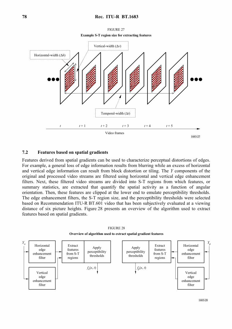
78 Rec. ITU-R BT.1683
1683-27
t t + 1 t + 2 t + 3 t + 4 t + 5
FIGURE 27Example S-T region size for extracting features
Video frames
Temporal-width (∆t)
Vertical-width (∆v)
Horizontal-width (∆h)
7.2 Features based on spatial gradients Features derived from spatial gradients can be used to characterize perceptual distortions of edges. For example, a general loss of edge information results from blurring while an excess of horizontal and vertical edge information can result from block distortion or tiling. The Y components of the original and processed video streams are filtered using horizontal and vertical edge enhancement filters. Next, these filtered video streams are divided into S-T regions from which features, or summary statistics, are extracted that quantify the spatial activity as a function of angular orientation. Then, these features are clipped at the lower end to emulate perceptibility thresholds. The edge enhancement filters, the S-T region size, and the perceptibility thresholds were selected based on Recommendation ITU-R BT.601 video that has been subjectively evaluated at a viewing distance of six picture heights. Figure 28 presents an overview of the algorithm used to extract features based on spatial gradients.
1683-28
Yo Yp
fo(s, t) fp(s, t)Vertical
edgeenhancement
filter
Horizontaledge
enhancementfilter
Extractfeatures
from S-Tregions
Applyperceptibility
thresholds
Applyperceptibility
thresholds
Extractfeatures
from S-Tregions
Verticaledge
enhancementfilter
Horizontaledge
enhancementfilter
FIGURE 28Overview of algorithm used to extract spatial gradient features

Rec. ITU-R BT.1683 79
7.2.1 Edge enhancement filters
The original and processed Y (luminance) video frames are first processed with horizontal and vertical edge enhancement filters that enhance edges while reducing noise. The two filters shown in Fig. 29 are applied separately, one to enhance horizontal pixel differences while smoothing vertically (left filter), and the other to enhance vertical pixel differences while smoothing horizontally (right filter).
1683-29
–WN –W2 –W1 0 W1 W2 WN
–WN –W2 –W1 0 W1 W2 WN
–WN –W2 –W1 0 W1 W2 WN
–WN –W2 –W1 0 W1 W2 WN
–WN –W2 –W1 0 W1 W2 WN
–WN –WN –WN
–W1
0 0 0 0 0 0 0
W1 W1
WN WN WN WN
–WN –WN –WN –WN
–W1 –W1 –W1 –W1–W1–W1
W1 W1 W1 W1 W1
WN WN WN
Ver
tical
low
pass
Horizontal bandpass
Ver
tical
ban
dpas
s
Horizontal lowpass
FIGURE 29Edge enhancement filters
The two filters are transposes of each other, have size 13 × 13, and have filter weights given by
−⋅
⋅=
2
21exp
cx
cxkwx
where: x : pixel displacement from the centre of the filter (0, 1, 2, …, N) c : constant that sets the width of the bandpass filter k : normalization constant selected such that each filter would produce the same
gain as a true Sobel filter [Jain, 1989].
The optimal amount of horizontal bandpass filtering for a viewing distance of six times picture height was found to be given by the c = 2 filter, which has a peak response at about 4.5 cycles/degree. The bandpass filter weights that were used are given by:
[–0.0052625, –0.0173446, –0.0427401, –0.0768961, –0.0957739, –0.0696751, 0, 0.0696751, 0.0957739, 0.0768961, 0.0427401, 0.0173446, 0.0052625]
Note that the filters in Fig. 29 have a flat low-pass response. A flat low-pass response produced the best quality estimate and has the added advantage of being computationally efficient (e.g. for the left filter in Fig. 29, one merely has to sum the pixels in a column and multiply once by the weight).
7.2.2 Description of features fSI13 and fHV13
This section describes the extraction of two spatial activity features from S-T regions of the edge-enhanced original and processed video streams from § 7.2.1. These features will be used to detect spatial impairments such as blurring and blocking. The filter shown in Fig. 29 (left) enhances

80 Rec. ITU-R BT.1683
spatial gradients in the horizontal, H, direction while the transpose of this filter (right) enhances spatial gradients in the vertical, V, direction. The response at each pixel from the H and V filters can be plotted on a two dimensional diagram such as the one shown in Fig. 30 with the H filter response forming the abscissa value and the V filter response forming the ordinate value. For a given image pixel located at row i, column j, and time t, the H and V filter responses will be denoted as H(i, j, t) and V(i, j, t), respectively. These responses can be converted into polar coordinates (R, θ) using the relationships:
22 ),,(),,(),,( tjiVtjiHtjiR +=
and (102)
=θ −),,(),,(tan),,( 1tjiHtjiVtji
The first feature is a measure of overall SI and hence is denoted as fSI13 since images were pre-processed using the 13 × 13 filter masks shown in Fig. 29. This feature is computed simply as the standard deviation (std) over the S-T region of the R(i, j, t) samples, and then clipped at the perceptibility threshold of P (i.e. if the result of the std calculation falls below P, fSI13 is set equal to P), namely
[ ] PSI tjiRf ),,(std13 = / region T-S,, ∈tji (103)
This feature is sensitive to changes in the overall amount of spatial activity within a given S-T region. For instance, localized blurring produces a reduction in the amount of spatial activity, whereas noise produces an increase. The recommended threshold P for this feature is 12.
1683-30
2∆θ
2∆θ
θ
H
V
R
V(i, j, t)
H(i, j, t)H
V
FIGURE 30Division of horizontal (H) and vertical (V) spatial activity into HV (left) and HV (right) distributions
rminrmin
The second feature, fHV13, is sensitive to changes in the angular distribution, or orientation, of spatial activity. Complementary images are computed with the shaded spatial gradient distributions shown in Fig. 30. The image with horizontal and vertical gradients, denoted as HV, contains the R(i, j, t) pixels that are horizontal or vertical edges (pixels that are diagonal edges are zeroed). The image with the diagonal gradients, denoted as HV , contains the R(i, j, t) pixels that are diagonal edges

Rec. ITU-R BT.1683 81
(pixels that are horizontal or vertical edges are zeroed). Gradient magnitudes R(i, j, t) less than rmin are zeroed in both images to assure accurate θ computations. Pixels in HV and HV can be represented mathematically as:
( )( ) ( ) ( ) ( )
=θ∆+π<θ<θ∆−π≥
=otherwise0
3,2,1,02
,,2
and,,if,,
,,
mmtjimrtjiRtjiR
tjiHV
min
(104)
and
( )( ) ( ) ( ) ( ) ( )
=θ∆−π+≤θ≤θ∆+π≥
=otherwise0
3,2,1,02
1,,2
and,,if,,
,,
mmtjimrtjiRtjiR
tjiHV
min
(105)
where:
region T-S,, ∈tji
For the computation of HV and HV above, the recommended value for rmin is 20 and the recommended value for ∆θ is 0.225 radians. Feature fHV13 for one S-T region is then given by the ratio of the mean of HV to the mean of ,HV where these resultant means are clipped at their perceptibility thresholds P, namely:
[ ]
[ ] P
PHV
tjiHV
tjiHVf
),,(mean
),,(mean13 = (106)
The recommended perceptibility threshold P for the mean of HV and HV is 3. The fHV13 feature is sensitive to changes in the angular distribution of spatial activity within a given S-T region. For example, if horizontal and vertical edges suffer more blurring than diagonal edges, fHV13 of the processed video will be less than fHV13 of the original video. On the other hand, if erroneous horizontal or vertical edges are introduced, say in the form of blocking or tiling distortions, then fHV13 of the processed video will be greater than fHV13 of the original video. The fHV13 feature thus provides a simple means to include variations in the sensitivity of the human visual system with respect to angular orientation10.
7.3 Features based on chrominance information
This section presents a single feature that can be used to measure distortions in the chrominance signals (CB, CR). For a given image pixel located at row i, column j, and time t, let CB (i, j, t) and CR (i, j, t) represent the Recommendation ITU-R BT.601 CB and CR values11. The components of a
10 This discussion of fHV13, though true in general, is somewhat simplified. For instance, when encountering
some shapes the fHV13 filter behaves in a manner that may be counter-intuitive (e.g. a corner formed by the joining of a vertical and horizontal line will result in diagonal energy).
11 Gain and offset corrections are not applied to the CB and CR image planes. See § 6.3.3.
82 Rec. ITU-R BT.1683
two-dimensional chrominance feature vector, fCOHER_COLOR, are computed as the mean, mean over the S-T region of the CB (i, j, t) and CR (i, j, t) samples, respectively, giving more perceptual weight to the CR component:
[ ] [ ]( ) 5.1and,regionST,,/),,(mean*,),,(mean_ =∈= RRRBCOLORCOHER WtjitjiCWtjiCf (107)
Equation (107) performs coherent integration (hence the name fCOHER_COLOR) since the phase relationship between CB and CR is preserved. If one is familiar with a vectorscope, the value of the chrominance feature when examining colour bar signals is readily apparent. For general-purpose scenes, one can visualize the chrominance feature vector’s usefulness for measuring distortions in chrominance for blocks of video that span a range of spatial and temporal extent. However, if S-T region size is too large, then many colours could be included in the calculation, and the usefulness of fCOHER_COLOR is reduced. An S-T region size of 8 horizontal pixels × 8 vertical lines × (1 to 3) video frames produces a robust chrominance feature vector (actually 4 horizontal CB and CR pixels, since these signals are sub-sampled by two in the horizontal direction for Recommendation ITU-R BT.601 sampling).
7.4 Features based on contrast information
Features that measure localized contrast information are sensitive to quality degradations such as blurring (e.g. contrast loss) and added noise (e.g. contrast gain). One localized contrast feature, fCONT, is easily computed for each S-T region from the Y luminance image as:
[ ] regionST,,/),,(std ∈= tjitjiYf PCONT (108)
The recommended perceptibility threshold P for the fCONT feature is between four and six.
7.5 Features based on ATI
Features that measure distortions in the flow of motion are sensitive to quality degradations such as dropped or repeated frames (motion loss) and added noise (motion gain). An ATI feature, fATI, is computed for each S-T region by first generating a motion video stream that is the absolute value of the difference between consecutive video frames at time t and t − 1, and then computing the standard deviation over the S-T region. Mathematically, this process will be represented as:
regionT-S,,/)1,,(),,( ∈−−= tjitjiYtjiYstdf PATI (109)
The recommended perceptibility threshold P for the fATI feature is between one and three.
The use of a previous frame introduces considerations beyond those required by the other features. When calculating fATI jointly with another feature (e.g. fCONTRAST_ATI from § 7.6) or for use in a model (see § 9), the requirement of an extra frame complicates the task of placement of S-T regions (see § 7.1.1).
7.6 Features based on the cross product of contrast and ATI
The perceptibility of spatial impairments can be influenced by the amount of motion that is present. Likewise, the perceptibility of temporal impairments can be influenced by the amount of spatial detail that is present. A feature derived from the cross product of contrast information and absolute
Rec. ITU-R BT.1683 83
temporal information can be used to partially account for these interactions. This feature, denoted as fCONTRAST_ATI, is computed as the product of the features in § 7.4 and 7.5 12. The recommended perceptibility threshold P = 3 is applied separately to each feature ( fCONT and fATI) before computing their cross product. Impairments will be more visible in S-T regions that have a low cross product than in S-T regions that have a high cross product. This is particularly true of impairments like noise and error blocks.
The requirement of an extra frame for fATI complicates fCONTRAST_ATI slightly, since the S-T regions used by both fCONT and fATI must be placed identically. Either one frame at the beginning of the video sequence must be left unused for fATI, or the S-T regions located at the beginning of the video sequence must contain one fewer frame (e.g. given a temporal extent of 6F, the first fATI S-T region would use 5F instead of 6F). The parameters and models specified herein presume the second solution will be used.
8 Quality parameters
8.1 Introduction Quality parameters that measure distortions in video quality due to gains and losses in the feature values are first calculated for each S-T region by comparing the original feature values, fo(s, t), with the corresponding processed feature values, fp(s, t) (§ 8.2). Several functional relationships are used to emulate the visual masking of impairments for each S-T region. Next, error-pooling functions across space and time emulate how humans deduce subjective quality ratings. Error pooling across space will be referred to as spatial collapsing (§ 8.3), and error pooling across time will be referred to as temporal collapsing (§ 8.4). Sequential application of the spatial and temporal collapsing functions to the stream of S-T quality parameters produces quality parameters for the entire video clip, which is nominally 5 to 10 s in duration. The final time-collapsed parameter values may be scaled and clipped (§ 8.5) to account for non-linear relationships between the parameter value and perceived quality and to further reduce the parameter’s sensitivity.
In summary, parameter calculations perform the following steps. Some features may not require the [Optional] step.
Step 1: Compare original feature values with processed feature values.
Step 2: Perform spatial collapsing.
Step 3: Perform temporal collapsing.
Step 4: [Optional] Perform non-linear scaling and/or clipping.
All parameters are designed to be either all positive or all negative. A parameter value of zero indicates no impairment.
8.2 Comparison functions The perceptual impairment at each S-T region is calculated using functions that model visual masking of the spatial and temporal impairments. This section presents the masking functions that are used by the various parameters to produce quality parameters as a function of space and time.
12 A standard cross product of the fCONT and fATI features (i.e. fCONT * fATI) is used for the processed fp(s, t) and
original fo(s, t) features in the ratio_loss and ratio_gain comparison functions described in § 8.2.1. However, for the log_loss and log_gain comparison functions, the processed and original features are computed as log10[fCONT] * log10[fATI], and the comparison functions use subtraction (i.e. fp(s, t) – fo(s, t) rather than log10[fp(s, t) / fo(s, t)]).
84 Rec. ITU-R BT.1683
8.2.1 Error ratio and logarithmic ratio
Loss and gain are normally examined separately, since they produce fundamentally different effects on quality perception (e.g. loss of spatial activity due to blurring and gain of spatial activity due to noise or blocking). Of the many comparison functions that have been evaluated, two forms have consistently produced the best correlation to subjective ratings. Each of these forms can be used with either gain or loss calculations for a total of four basic S-T comparison functions. The four primary forms are:
−
=),(
),(),(),(ratio_loss
tsftsftsf
nptso
op
−
=),(
),(),(),(ratio_gain
tsftsftsf
pptso
op
=
),(),(
log),loss(log_ 10 tsftsf
nptso
p
=
),(),(
log),gain(log_ 10 tsftsf
pptso
p
where:
pp : positive part operator (i.e. negative values are replaced with zero)
np : negative part operator (i.e. positive values are replaced with zero).
These visual masking functions imply that impairment perception is inversely proportional to the amount of localized spatial or temporal activity that is present. In other words, spatial impairments become less visible as the spatial activity increases (i.e. spatial masking), and temporal impairments become less visible as the temporal activity increases (i.e. temporal masking). While the logarithmic and ratio comparison functions behave very similarly, the logarithmic function tends to be slightly more advantageous for gains while the ratio function tends to be slightly more advantageous for losses. The logarithm function has a larger dynamic range, and this is useful when the processed feature values greatly exceed the original feature values.
8.2.2 Euclidean distance
Another useful S-T comparison function is simple Euclidean distance, represented by the length of the difference vector between the original feature vector fo(s, t) and the corresponding processed feature vector, fp(s, t):
)()()euclid( s,tfs,tfs,t op −= (110)
Figure 31 gives an illustration of Euclidean distance for a two-dimensional feature vector extracted from an S-T region (e.g. the fCOHER_COLOR feature vector of § 7.3), where s and t are indices that denote the spatial and temporal positions, respectively, of the S-T region within the calibrated original and processed video streams. The dashed line in Fig. 31 shows the Euclidean distance. The Euclidean distance measure can be generalized for feature vectors that have an arbitrary number of dimensions.

Rec. ITU-R BT.1683 85
1683-31
fp (s, t)
fo (s, t)
FIGURE 31Illustration of the Euclidean distance euclid (s, t) for a two-dimensional feature vector
Dimension 1
Dimension 2
euclid (s, t)
8.3 Spatial collapsing functions
The parameters from the S-T regions (from § 8.2) form three-dimensional matrices spanning one temporal axis and two spatial dimensions (i.e. horizontal and vertical placement of the S-T region). Next, impairments from the S-T regions with the same time index t are pooled using a spatial collapsing function. Spatial collapsing yields a time history of parameter values. This time history of parameter values, denoted generically as p(t), must then be temporally collapsed using a temporal collapsing function given in § 8.4. Table 12 presents a summary of the most commonly used spatial collapsing functions.
Extensive investigation has revealed that the optimal spatial collapsing functions normally involve some form of worst case processing, like the average of the worst 5% of the distortions observed over the spatial index s [Wolf and Pinson, 1998, 1999, 2001 and June 2002]. This is because localized impairments tend to draw the focus of the viewer, making the worst part of the picture the predominant factor in the subjective quality decision. For example, the spatial collapsing function above95% is computed at each temporal index t for the log_gain(s, t) function in § 8.2.1 as the average of the most positive 5% of the values over the spatial index s 13. This amounts to sorting the gain distortions from low to high at each temporal index t and averaging those distortions that are above the 95% threshold (since more positive values imply greater distortion). Similarly, loss distortions such as those produced by the ratio_loss(s, t) function in § 8.2.1 would be sorted at each temporal index t, but the average of those distortions that are below5% is used (since losses are negative).
8.4 Temporal collapsing functions
The parameter time history results p(t) output from the spatial collapsing function (from § 8.3) are next pooled using a temporal collapsing function to produce an objective parameter p for the video clip, which is nominally 4 to 10 s in length. Viewers seem to use several temporal collapsing
13 Notice that the time index, t, does not indicate individual frames (see § 7.1.1) here. Instead, each value of t
corresponds to those S-T regions having the same time extent.

86 Rec. ITU-R BT.1683
functions when subjectively rating video clips that are approximately 10 s in length. The mean over time is indicative of the average quality that is observed during the time period. The 90% and 10% levels over time are indicative of the worst transient quality that is observed for gains and losses, respectively (e.g. digital transmission errors may cause a 1 to 2 s disturbance in the processed video). After temporal collapsing, a given parameter p is either all negative or all positive, but not both. Table 13 presents a summary of the most commonly used temporal collapsing functions.
TABLE 12
Spatial collapsing functions and their definitions
Spatial collapsing function Definition
below5% For each temporal index t, sort the parameter values from low to high. Compute the average of all the parameter values that are less than or equal to the 5% threshold level. For loss parameters, this spatial collapsing function produces a parameter that is indicative of the worst quality over space
above95% For each temporal index t, sort the parameter values from low to high. Compute the average of all the parameter values that are greater than or equal to the 95% threshold level. For gain parameters, this spatial collapsing function produces a parameter that is indicative of the worst quality over space
mean For each temporal index t, compute the average of all the parameter values. This spatial collapsing function produces a parameter that is indicative of the average quality over space
std For each temporal index t, compute the standard deviation of all the parameter values. This spatial collapsing function produces a parameter that is indicative of the quality variations over space
below5%tail For each temporal index t, sort the parameter values from low to high. Compute the average of all the parameter values that are less than or equal to the 5% threshold level, and then subtract the 5% level from this average. For loss parameters, this spatial collapsing function allows one to measure the spread of the worst quality levels over space. It is useful for measuring the perceptual quality effects of spatially localized distortions
above99%tail For each temporal index t, sort the parameter values from low to high. Compute the average of all the parameter values that are greater than or equal to the 99% threshold level, and then subtract the 99% level from this average. For gain parameters, this spatial collapsing function allows one to measure the spread of the worst quality levels over space. It is useful for measuring the perceptual quality effects of spatially localized distortions

Rec. ITU-R BT.1683 87
8.5 Non-linear scaling and clipping
The all-positive or all-negative temporally collapsed parameter p from § 8.4 may be scaled to account for non-linear relationships between the parameter value and perceived quality. It is preferable to remove any non-linear relationships before building the video quality models (§ 9), since a linear least-squares algorithm will be used to determine the optimal parameter weights. The two non-linear scaling functions that might be applied are the square root function, denoted by sqrt, and the square function, denoted by square. If the sqrt function is applied to an all-negative parameter, the parameter is first made all positive (i.e. absolute value taken).
Finally, a clipping function denoted as clip_T, where T is the clipping threshold, might be applied to reduce the sensitivity of the parameter to small impairments. The clipping function replaces any
TABLE 13
Temporal collapsing functions and their definitions
Temporal collapsing function Definition
10% Sort the time history of the parameter values from low to high and select the 10% threshold level. For loss parameters, this temporal collapsing function produces a parameter that is indicative of the worst quality over time. For gain parameters, it produces a parameter that is indicative of the best quality over time
25% Sort the time history of the parameter values from low to high and select the 25% threshold level
50% Sort the time history of the parameter values from low to high and select the 50% threshold level
90% Sort the time history of the parameter values from low to high and select the 90% threshold level. For loss parameters, this temporal collapsing function produces a parameter that is indicative of the best quality over time. For gain parameters, it produces a parameter that is indicative of the worst quality over time
mean Compute the mean of the time history of the parameter values. This produces a parameter that is indicative of the average quality over time
std Compute the standard deviation of the time history of the parameter values. This temporal collapsing function produces a parameter that is indicative of the quality variations over time
above90%tail Sort the time history of the parameter values from low to high and compute the average of all the parameter values that are greater than or equal to the 90% threshold level, and then subtract the 90% level from this average. For gain parameters, this temporal collapsing function allows one to measure the spread of the worst quality levels over time. It is useful for measuring the perceptual quality effects of temporally localized distortions
88 Rec. ITU-R BT.1683
parameter value between the clipping level and zero with the clipping level, and then the clipping level is subtracted from all resulting parameter values. This is represented mathematically as:
( )
−−
=negativeallisifpositiveallisif
,min),max(
)clip_T(pp
TTpTTp
p
8.6 Parameter naming convention This section summarizes the technical naming convention used for video quality parameters. This convention assigns to each parameter a lengthy name consisting of identifying words (sub-names) separated by underscores. The technical parameter name summarizes the exact process used to calculate the parameter. Each sub-name identifies one function or step in the process of calculating the parameter. Sub-names are listed in the order in which they occur, from left to right. Table 14 summarizes the sub-names used to create the technical parameter name, listed in the order that they occur. Paragraph 8.6.1 provides examples of technical parameter names and their associated sub-names from Table 14.
TABLE 14
Technical naming convention used for video quality parameters
Sub-name Definition Examples
Colour The colour space image planes used by the parameter Y for luminance image plane. color for (CB, CR) image planes
Feature Specific
The “Feature Specific” sub-name describes the calculations that make this parameter unique. All other sub-names that follow are generic processes that can be used by many different types of parameters. The “Feature Specific” sub-name is usually the name of the feature that is extracted from the “Colour” plane at this point in the flow, hence the location of this sub-name. However, information not otherwise covered by the naming convention can also be included here. For example, the HV parameter applies the “Block Statistic” sub-name separately to the HV and HV image planes. The subsequent ratio of HV to HV is specified by the “Feature Specific” sub-name (i.e. rather than occupying a separate sub-name after the “Block Statistic”)
si13 for the fSI13 feature in § 7.2.2. hv13_angleX.XXX_rmin YY for the fHV13 feature in § 7.2.2, where X.XXX is ∆θ and YY is the rmin. coher_color for the fCOHER_COLOR feature in § 7.3. cont: for the fCONT feature in § 7.4. ati: for the fATI feature in § 7.5. contrast_ati: for the fCONTRAST_ATI feature in § 7.6
Block Shift Present when S-T blocks slide (e.g. overlap in time). When absent, blocks are assumed to abut in time
sliding
Full Image Present when the S-T block size contains the entire valid region of the image. When absent, the “Block Size” sub-name must be present
image

Rec. ITU-R BT.1683 89
TABLE 14
Technical naming convention used for video quality parameters
Sub-name Definition Examples
Block Size Present when the image is divided into S-T blocks (see § 7.1.1). For consistency, block size is always indicated relative to the luminance (Y ) plane’s frame lines and frame pixels. Thus, for 4:2:2 sampled video, colour blocks will actually contain half the specified number of pixels horizontally. When absent, the “Full Image” sub-name must be present
8 × 8: for blocks that include 8 frame lines vertically by 8 frame pixels horizontally. 128 × 128: for blocks that include 128 frame lines vertically by 128 frame pixels horizontally
Block Frames Indicates the temporal extent of the S-T blocks (see § 7.1.1), referenced to 30 fps video. For example, 6F is used to represent one fifth of a second, regardless of the frame rate of the video being measured (e.g. 5 frames from a 25 fps system, 3 frames from a 15 fps system, 2 frames from a 10 fps system)
1F: for a temporal extent of one frame. 6F: for a temporal extent of one fifth of a second
Block Statistic The statistical function used to extract the feature from each S-T region, producing one number for each S-T block of pixels. Present unless “Block Size” = 1 × 1 (i.e. 1 pixel). Before the Block Statistic has been applied, intermediate results contain time histories of images with one number per pixel (i.e. filtered images); afterward, intermediate results contain one number per each S-T region (i.e. feature images). Parameters that have two image planes (e.g. hv13 and coher_color) will apply the Block Statistic separately to both image planes, producing two feature images
mean is the average of the pixel values. std is the standard deviation of the pixel values. rms is the root mean square of the pixel values
Perceptibility Threshold
The values produced by the “Block Statistic” may be clipped at a perceptibility threshold P. Values between zero and this threshold are replaced with the threshold
3 for a minimum feature value of 3.0. 12 for a minimum feature value of 12.0
Comparison Function
The function used to compare features extracted from the original and processed feature streams (see § 8.2). Before the “Comparison Function”, the intermediate results contain time histories of original and processed feature images; afterward the intermediate results contain a time history of parameter images
log_gain (see § 8.2.1). ratio_loss (see § 8.2.1). euclid (see § 8.2.2)
Spatial Collapsing Function
See § 8.3. The function is applied to each parameter image (e.g. all S-T regions having the same temporal index) and produces a time history of parameter values. Before spatial collapsing, intermediate results consist of parameter images containing one value for each S-T block; afterward, intermediate results are a time history of numbers (i.e. parameter time history). Must be present for all parameters except “Full Image” parameters
See Table 12

90 Rec. ITU-R BT.1683
TABLE 14
Technical naming convention used for video quality parameters
Sub-name Definition Examples
Temporal Collapsing Function
See § 8.4. The function is applied to the parameter time history and produces one parameter value for the entire video sequence. After temporal collapsing, the parameter contains either all negative values or all positive values, but not both. Zero is associated with no impairment, and parameter values further from zero have higher impairments. Must be present for all parameters
See Table 13
Non-linear Function
See § 8.5. Examination of the parameter’s values may indicate that the parameter should be scaled in a non-linear fashion to linearly track the subjective data. The Non-linear Function performs this final scaling. If the sqrt function is applied to an all-negative parameter, the parameter is first made all positive (i.e. absolute value taken)
sqrt for the square root of the temporally collapsed parameter value. square for the square of the temporally collapsed parameter value
Clipping Function
See § 8.5. Final examination of the parameter values may indicate a need to further reduce the sensitivity of the parameter to small impairments (e.g. parameter values near zero). Replace any value between the clipping level T and zero with the clipping level, and then subtract the clipping level from all resulting parameter values
clip_0.45 If parameter values are positive, replace all values less than 0.45 with 0.45 and then subtract 0.45 from all the parameter values. If parameter values are negative, replace all values greater than –0.45 with –0.45 and then add 0.45 to all the parameter values
8.6.1 Example parameter names
This section includes five example technical names, and a step-by-step description of the sub-naming procedure given in Table 14.
Y_si13_8×8_6F_std_6_ratio_loss_below5%_mean
Y means that the luminance image plane is used. si13 represents filtering of those images with the 13 × 13 spatial masks in § 7.2.1 in preparation for extraction of the fSI13 feature in § 7.2.2. 8 × 8_6F represents dividing the video stream into S-T regions containing eight frame lines vertically by eight pixels horizontally by one fifth of a second temporally (i.e. 6 NTSC frames, 5 PAL frames). std represents taking the standard deviation of each block. 6 represents application of a perceptibility threshold, replacing all standard deviation values below 6.0 with a value of 6.0. ratio_loss represents comparing the original and processed features from each block using the ratio_loss function. below5% represents spatially collapsing the parameter values at each time index using the below5% function. mean represents temporally collapsing the parameter time history using the mean function.
color_coher_color_8×8_1F_mean_euclid_std_10%_clip_0.8

Rec. ITU-R BT.1683 91
color represents using the CB and CR image planes. coher_color represents preservation of the phase relationship between the CB and CR images (by treating them separately) in preparation for extraction of the fCOHER_COLOR feature in § 7.3. 8 × 8_1F represents dividing each frame into blocks that are 8 frame lines high by 4 CB and CR pixels wide (due to 4:2:2 sub-sampling of the CB and CR image planes) by 1 frame in time. mean represents taking the mean value of each block. euclid represents computing the Euclidean distance between original vectors (CB, CR) and processed vectors (CB, CR) for each S-T block. std represents the std spatial collapsing function. 10% represents the 10% temporal collapsing function. clip_0.8 represents clipping the final parameter value at a minimum of 0.8 (i.e. replacing all values below 0.8 with 0.8, and then subtracting 0.8).
Y_hv13_angle0.225_rmin20_8×8_6F_mean_3_ratio_loss_below5%_mean_square_clip_0.05
Y means that the luminance image plane is used. hv13 represents filtering of the Y images with the 13 × 13 spatial masks in § 7.2.1 in preparation for extraction of the fHV13 feature in § 7.2.2 (i.e. the HV and HV images are created and treated separately until after the Perceptibility Threshold). angle0.225 and rmin20 represent a ∆θ of 0.225 radians and an rmin of 20 for calculation of the fHV13 feature. 8 × 8_6F represents dividing the video stream into S-T regions containing eight frame lines vertically by eight pixels horizontally by one-fifth of a second temporally (i.e. 6 NTSC frames, 5 PAL frames). mean represents taking the mean value of each S-T block for HV and .HV 3 represents the application of a perceptibility threshold to these means, replacing all values less than 3 with 3.0. Next, the fHV13 feature in § 7.2.2 is calculated as the ratio of clipped means of HV to the clipped means of HV , as specified in hv13_angle0.225_rmin20, the Feature Specific sub-name. ratio_loss represents using the ratio_loss comparison function for each original and corresponding processed fHV13 feature extracted from an S-T block. below5% specifies the spatial collapsing function. mean specifies the temporal collapsing function. square specifies the non-linear function for each time-collapsed parameter value. clip_0.05 represents the clipping function, where all values below 0.05 are replaced with 0.05, and then 0.05 is subtracted from the result (recall that the all-negative parameter will become an all-positive parameter due to the non-linear function, square).
Y_contrast_ati_4×4_6F_std_3_ratio_gain_mean_10%
Y means the luminance plane is used. contrast_ati represents computing two separate filtered versions of the image in preparation for extraction of the fCONTRAST_ATI feature in § 7.6. The first filter, contrast, will consider the luminance planes directly (§ 7.4). The second filter, ati, will consider images generated by taking differences between successive luminance planes (§ 7.5). The contrast and ati images are treated separately until after the thresholding. 4 × 4_6F means that the two video streams are divided into S-T regions containing four frame lines vertically by four pixels horizontally by one-fifth of a second temporally (e.g. 6 NTSC frames, 5 PAL frames). The first S-T block of ati images will actually contain only 5 images rather than 6 since an ati image cannot be generated for the first frame in the sequence (i.e. there is no earlier image in time available). This exception is specified as part of the Feature Specific sub-name. std represents taking the standard deviation of each block. Then, as specified in the Feature Specific sub-name in § 7.6, apply a perceptibility threshold of 3 to both the contrast and ati features (replace all values less than 3 with 3.0). Next, multiply the contrast block-value with the ati block-value for each S-T block (see footnote in § 7.6 for special instructions on how to perform this multiplication) and continue calculations with this combined feature image. ratio_gain is the comparison function used to compare each original and processed feature from the S-T blocks. mean is the spatial collapsing function. 10% is the temporal collapsing function.

92 Rec. ITU-R BT.1683
9 General model
This section provides a full description of the general model VQM (denoted as VQMG). The general model is optimized to achieve maximum objective to subjective correlation using a wide range of video quality and bit rates. The general model has objective parameters for measuring the perceptual effects of a wide range of impairments such as blurring, block distortion, jerky/unnatural motion, noise (in both the luminance and chrominance channels), and error blocks (e.g. what might typically be seen when digital transmission errors are present). This model consists of a linear combination of video quality parameters whose naming conventions are described in § 8.6. The selection of video quality parameters was determined by the optimization criteria given above. The general model produces output values that range from zero (no perceived impairment) to approximately one (maximum perceived impairment). To place results on the double stimulus continuous quality scale (DSCQS), multiply VQMG by 100.
The general model was designed based on Recommendation ITU-R BT.601 video that has been subjectively evaluated at a viewing distance of six picture heights. When analysing video sequences for different viewing distances, a scaling factor must be applied to the results. As viewing distance increases, impairments become less visible; as viewing distance decreases, impairments become more visible. Care should be taken when comparing results for video sequences that will be viewed at different viewing distances.
VQMG consists of a linear combination of seven parameters. Four parameters are based on features extracted from spatial gradients of the Y luminance component (§ 7.2.2), two parameters are based on features extracted from the vector formed by the two chrominance components (CB, CR) (§ 7.3), and one parameter is based on contrast and absolute temporal information features, both extracted from the Y luminance component (§ 7.4 and 7.5, respectively). VQMG is given by:
VQMG = –0.2097 * Y_si13_8×8_6F_std_12_ratio_loss_below5%_10%
+0.5969 * Y_hv13_angle0.225_rmin20_8×8_6F_mean_3_ratio_loss_below5%_mean_square_clip_0.06
+0.2483 * Y_hv13_angle0.225_rmin20_8×8_6F_mean_3_log_gain_above95%_mean
+0.0192 * color_coher_color_8×8_1F_mean_euclid_std_10%_clip_0.6
–2.3416 * [Y_si13_8×8_6F_std_8_log_gain_mean_mean_clip_0.004 | 0.14]
+0.0431 * Y_contrast_ati_4×4_6F_std_3_ratio_gain_mean_10%
+0.0076 * color_coher_color_8×8_1F_mean_euclid_above99%tail_std | 0.0
Remember, that the above features for the general model with a “6F” time extent will actually contain five PAL (625-line) video frames.
The square on the hv_loss parameter is necessary to linearize the parameter response with respect to the subjective data. Note that since the hv_loss parameter becomes positive after the square, a positive multiplying weight is used. Also note that the hv_loss parameter is clipped at 0.06, the colour parameter is clipped at 0.6, and the si_gain parameter is clipped at 0.004. The si_gain parameter is the only quality improvement parameter in the model (since the si_gain parameter is positive, a negative weight results in negative contributions to VQM which produce quality improvements). The si_gain parameter measures improvements to quality that result from edge sharpening or enhancement. Clipping of the parameter at an upper threshold of 0.14 immediately before multiplying by the parameter weight prevents excessive improvements to VQM of more than about 1/3 of a quality unit, which is the maximum improvement observed in the general subjective data set (i.e. an HRC will only be rewarded for a little edge enhancement).
The total VQM (after the contributions of all the parameters are added up) is clipped at a lower threshold of 0.0 to prevent negative VQM numbers. Finally, a crushing function that allows a

Rec. ITU-R BT.1683 93
maximum of 50% overshoot is applied to VQM values over 1.0 to limit VQM values for excessively distorted video that falls outside the range of the currently available subjective data.
If VQMG > 1.0, then VQMG = (1 + c) * VQMG / (c + VQMG), where c = 0.5.
VQMG computed in the above manner will have values greater than or equal to zero and a nominal maximum value of one. VQMG may occasionally exceed one for video scenes that are extremely distorted.
10 References
JAIN, A. K. [1989] Fundamentals of Digital Image Processing. Englewood Cliffs, NJ: Prentice-Hall Inc., 1989, p. 348-357.
PINSON, M. and WOLF, S. [February 2002] Video Quality Measurement User’s Manual. NTIA Handbook 02-1. National Telecommunications and Information Administration.
SMPTE [1995a] SMPTE 125M. Television – Component Video Signal 4:2:2 – Bit-Parallel Digital Interface. Society of Motion Picture and Television Engineers, 595 West Hartsdale Avenue, White Plains, NY 10607.
SMPTE [1995b] SMPTE Recommended Practice 187. Center, Aspect Ratio, and Blanking of Video Images. Society of Motion Picture and Television Engineers, 595 West Hartsdale Avenue, White Plains, NY 10607.
SMPTE [1999] SMPTE 170M. SMPTE Standard for Television – Composite Analog Video Signal – NTSC for Studio Applications. Society of Motion Picture and Television Engineers, 595 West Hartsdale Avenue, White Plains, NY 10607.
WOLF, S. and PINSON, M. [12-13 November 1998] In-service performance metrics for MPEG-2 video systems. Proc. Made to Measure 98 – Measurement Techniques of the Digital Age Technical Seminar, technical conference jointly sponsored by the International Academy of Broadcasting (IAB), the ITU, and the Technical University of Braunschweig (TUB), Montreux, Switzerland.
WOLF, S. and PINSON, M. [September 1999] Spatial-temporal distortion metrics for in-service quality monitoring of any digital video system. Proc. SPIE International Symposium on Voice, Video, and Data Communications, Boston, MA.
WOLF, S. and PINSON, M. [July 2001] The relationship between performance and spatial-temporal region size for reduced-reference, in-service video quality monitoring systems. Proc. SCI/ISAS 2001 (Systematics, Cybernetics, and Informatics/Information Systems Analysis and Synthesis), p. 323-328. National Telecommunications and Information Administration.
WOLF, S. and PINSON, M. [June 2002] Video Quality Measurement Techniques. NTIA Report 02-392.
Annex 5a
NTIA VQM raw objective data
This Annex provides a full disclosure of the NTIA VQM raw objective data.
Raw data summary
This General Model developed by the NTIA was originally designed to output values on a nominal 0 to 1 scale, where 0 represents no perceived impairment and 1 represents maximum perceived impairment. However, the binary executable submitted to the VQEG Phase II FR-TV test

94 Rec. ITU-R BT.1683
transformed the (0, 1) values of the General Model to (0, 100) to match the DSCQS. Since all model values should now be scaled to (0, 1), we have removed the 100 times multiplication factor (i.e. multiplication by 100) to restore the original (0, 1) scale of the General Model.
The General Model values calculated here used the centre 8 s of video in each clip, discarding the 10 extra frames of video at the beginning and end of each video file as described in the VQEG Phase II FR-TV Test Plan. For the calibration routines, an uncertainty of 30 frames and a frequency of 15 frames were used (see § 6 of Annex 5). In addition, the SROI used to calculate the VQM value for each clip was chosen as follows:
Step 1: For 525-line video systems, use a default SROI of 672 pixels × 448 lines centred in the video frame. For 625-line video systems, use a default SROI of 672 pixels × 544 lines centred in the video frame. These SROI defaults may be modified as given in Steps 2 and 3.
Step 2: The model requires 6 additional valid pixels/lines on all sides of the above SROI for the spatial filters to operate properly. If the PVR (calculated automatically as given in § 6.2 of Annex 5) is not large enough to encompass the default SROI plus 6 pixels/lines (Step 1), then the SROI is reduced by multiples of 8 pixels/lines only in the necessary direction (horizontal or vertical).
Step 3: The SROI is always centred horizontally such that the left hand sample starts at Recommendation UIT-R BT.601 luminance/chrominance co-located sampling point. The SROI is centred vertically such that when separated into two fields, the same number of lines is discarded from the top of each field. If the SROI has been reduced in size in Step 2, then perfect centring of the SROI within the video frame may not be possible.
Evaluation software that implements the General Model and its calibration routines may be downloaded from:
http://www.its.bldrdoc.gov/n3/video/vqmsoftware.htm

Rec. ITU-R BT.1683 95
TABLE 15
525-line raw objective data
Source No. HRC No. NTIA: Proponent H
1 1 0.660 (1)
1 2 0.347 1 3 0.286 1 4 0.178 2 1 0.449 2 2 0.246 2 3 0.119 2 4 0.061 3 1 0.321 3 2 0.167 3 3 0.076 3 4 0.049 4 5 0.396 4 6 0.280 4 7 0.222 4 8 0.183 5 5 0.329 5 6 0.217 5 7 0.159 5 8 0.115 6 5 0.542 6 6 0.266 6 7 0.189 6 8 0.139 7 5 0.258 7 6 0.161 7 7 0.108 7 8 0.076 8 9 0.911 8 10 0.717 8 11 0.721 8 12 0.526 8 13 0.424 8 14 0.311 9 9 0.827 9 10 0.453 9 11 0.512 9 12 0.264 9 13 0.188 9 14 0.124
10 9 0.666 10 10 0.250
10 11 0.375 10 12 0.129 10 13 0.078 10 14 0.153 11 9 0.513 11 10 0.534 11 11 0.407 11 12 0.161 11 13 0.148 11 14 0.159 12 9 0.600 12 10 0.410 12 11 0.471 12 12 0.244 12 13 0.171 12 14 0.114 13 9 0.537 13 10 0.425 13 11 0.346 13 12 0.215 13 13 0.188 13 14 0.169
(1) For Source 1, HRC 1, the calibration software
submitted to VQEG produced a spatial/temporal registration error that incorrectly estimated the processed video to be reframed (i.e. shifted by one field, see § 6.1.2 in Annex 5). For the other scenes of HRC 1, spatial/temporal registration was correctly estimated. § 6.1.5.7 in Annex 5, recommends median filtering of the calibration results over all scenes of a given HRC as a method to produce more robust calibration estimates for a given HRC. However, the VQEG Phase II test plan specified that all VQM software produce a single quality estimate for each clip independently. Thus, median filtering of calibration numbers over all scenes for a given HRC was not allowed by the test plan. Had median filtering of calibration numbers been allowed, the VQM software would have correctly registered this clip and the raw objective score would have been 0.529.
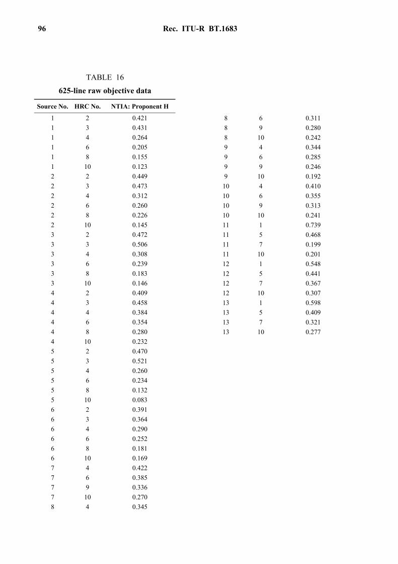
96 Rec. ITU-R BT.1683
TABLE 16
625-line raw objective data
Source No. HRC No. NTIA: Proponent H
1 2 0.421 1 3 0.431 1 4 0.264 1 6 0.205 1 8 0.155 1 10 0.123 2 2 0.449 2 3 0.473 2 4 0.312 2 6 0.260 2 8 0.226 2 10 0.145 3 2 0.472 3 3 0.506 3 4 0.308 3 6 0.239 3 8 0.183 3 10 0.146 4 2 0.409 4 3 0.458 4 4 0.384 4 6 0.354 4 8 0.280 4 10 0.232 5 2 0.470 5 3 0.521 5 4 0.260 5 6 0.234 5 8 0.132 5 10 0.083 6 2 0.391 6 3 0.364 6 4 0.290 6 6 0.252 6 8 0.181 6 10 0.169 7 4 0.422 7 6 0.385 7 9 0.336 7 10 0.270 8 4 0.345
8 6 0.311 8 9 0.280 8 10 0.242 9 4 0.344 9 6 0.285 9 9 0.246 9 10 0.192
10 4 0.410 10 6 0.355 10 9 0.313 10 10 0.241 11 1 0.739 11 5 0.468 11 7 0.199 11 10 0.201 12 1 0.548 12 5 0.441 12 7 0.367 12 10 0.307 13 1 0.598 13 5 0.409 13 7 0.321 13 10 0.277
Rec. ITU-R BT.1683 97
Appendix 1
Results of the Video Quality Expert Group FR-TV Phase II test
Introduction
The performance of the perceptual quality models included in this Recommendation was assessed through two parallel evaluations. In the first evaluation, a standard subjective method, the DSCQS method, was used to obtain subjective ratings of quality of video material by panels of human observers. In the second evaluation, objective ratings were obtained by the objective computational models. For each model, several metrics were computed to measure the accuracy and consistency with which the objective ratings predicted the subjective ratings.
This Appendix describes the subjective evaluation portion of the test as well as the results for the objective computational models submitted by the following proponents:
– Model 1 (British Telecom; identified in VQEG FR-TV Phase II as Proponent D);
– Model 2 (Yonsei University/Radio Research Laboratory/SK Telecom; identified in VQEG FR-TV Phase II as Proponent E);
– Model 3 (CPqD; identified in VQEG FR-TV Phase II as Proponent F);
– Model 4 (NTIA; identified in VQEG FR-TV Phase II as Proponent H).
Three independent laboratories conducted the subjective tests. Two laboratories, Communications Research Center (CRC, Canada) and Verizon (United States of America), performed the test with 525/60 Hz sequences and a third lab, Fondazione Ugo Bordoni (FUB, Italy), performed the test with 625/50 Hz sequences.
A detailed description of the Video Quality Expert Group FR-TV Phase II test is provided in the mentionned Document1.
2 Video materials
The 525/60 or 625/50 line formats test video sequences were in Recommendation ITU-R BT.601 4:2:2 component video format using an aspect ratio of 4:3.
2.1 SRC and HRC
For each of the 525 and 625 tests, thirteen SRCs with different characteristics (e.g. format, temporal and spatial information, colour, etc.) were used (see Tables 17 and 18).
In both tests, the HRCs were chosen to represent typical conditions of secondary distribution of digitally encoded television quality video. In the 625 test, ten HRCs were used; their characteristics are presented in Table 19. In the 525 test, fourteen HRCs were used; their characteristics are presented in Table 20.
In both 625 and 525 tests, SRCs and HRCs were combined into a sparse matrix (see Tables 23-26).

98 Rec. ITU-R BT.1683
TABLE 17
625/50 format sequences (SRCs)
SRC number Characteristics
1 View of skyline taken from moving boat; originated as 16:9 film, telecined to 576i/50
2 Dancers on wood floor with fast motion, moderate detail; originally captured in D5 format
3 Indoor men’s volleyball match; captured in D5 format
4 Women’s soccer game action with fast camera panning; captured in D5
5 12 fps traditional animation; source converted to 24 fps film, then telecined to 576i/50
6 Slowly rotating wireframe globe; captured in DigiBetaCam
7 Rapid in-scene and camera motion, with lighting effects
8 Close-up of guitar being played, with changing light effects
9 Colour, motion, detail
10 High detail, textured background, motion
11 Colour, motion, detail
12 Outdoor rugby match; movement, colour
13 Motion, details, moving water
14 (demo) Rapid in-scene and camera motion, with lighting effects
15 (demo) Rapid in-scene and camera motion, with lighting effects
16 (demo) Facial close-up followed by wide shot of construction site

Rec. ITU-R BT.1683 99
TABLE 19
625/50 HRCs
HRC number Bit rate Resolution Method Comments
1 768 kbit/s CIF H.263 Full screen (HRC15 from VQEG 1) 2 1 Mbits/s 320H MPEG2 Proponent encoded 3 1.5 Mbit/s 720H MPEG2 Encoded by FUB 4 2.5 4 Mbit/s 720H MPEG2 Cascaded by FUB 5 2 Mbit/s 3/4 MPEG2, sp@ml HRC13 from VQEG 1 6 2.5 Mbit/s 720H MPEG2 Encoded by FUB 7 3 Mbit/s full MPEG2 HRC9 from VQEG 1 8 3 Mbit/s 704H MPEG2 Proponent encoded 9 3 Mbit/s 720H MPEG2 Encoded by FUB
10 4 Mbit/s 720H MPEG2 Encoded by FUB
TABLE 18
525/60 format sequences (SRCs)
SRC number Characteristics
1 Outdoor football match, with colour, motion, textured background 2 Autumn landscape with detailed colour, slow zooming 3 Animation containing movement, colour and scene cuts 4 Highly detailed park scene with water; down converted from HDTV source 5 Colour and rapid motion; down converted from HDTV 6 Colour, large water surface; down converted from HDTV 7 Neighbourhood soccer match, moderate motion; down converted from HDTV 8 Water amusement park; (DigiBetaCam) 9 Amusement park ride with moderate motion, high detail, slow zoom; (DigiBetaCam)
10 Colour, motion, moderately low illumination; (DigiBetaCam) 11 12 fps traditional animation, converted to 24 fps film and telecined to 480i/60 12 Detailed outdoor fountain with camera zoom; (DigiBetaCam) 13 Scene cuts from close-up of engine ignition, to distant wide shot, and back; film original
telecined to 480i/60 14 (demo) Close-up shot of a rose in light breeze; motion, colour and detail; (DigiBetaCam) 15 (demo) High detail, low motion; downconverted from HDTV 16 (demo) Slowly rotating statues, swaying tree branches; (DigiBetaCam)

100 Rec. ITU-R BT.1683
TABLE 20
525/60 HRCs
HRC number Bit rate Resolution Method Comments
1 768 kbit/s CIF H.263 Full screen (HRC15 from VQEG 1) 2 2 Mbit/s 3/4 MPEG2, sp@ml HRC13 from VQEG 1 3 3 Mbit/s full MPEG2 HRC9 from VQEG 1 4 5 Mbit/s 720H MPEG2 Encoded by CRC 5 2 Mbit/s 704H MPEG2 Encoded by CRC 6 3 Mbit/s 704H MPEG2 Encoded by CRC 7 4 Mbit/s 704H MPEG2 Encoded by CRC 8 5 Mbit/s 704H MPEG2 Encoded by CRC 9 1 Mbit/s 704H MPEG2 Proponent encoded; low-bit rate
combined with high resolution 10 1 Mbit/s 480H MPEG2 Encoded by CRC; low-bit rate, low
resolution 11 1.5 Mbit/s 528H MPEG2 Proponent encoded; 64-QAM
modulation; composite NTSC output converted to component
12 4 2 Mbit/s 720H MPEG2 Proponent encoded; cascaded encoders 13 2.5 Mbit/s 720H MPEG2 Encoded by CRC 14 4 Mbit/s 720H MPEG2 Proponent encoded; using software
codec
1 Methodology for the evaluation of objective model performance
The DSCQS method of Recommendation ITU-R BT.500 was used for subjective testing. For the 525 test, difference mean opinion scores (DMOS) were collected for 63 SRC×HRC combinations. For the 625, DMOS were collected for 64 SRC×HRC combinations. For the same SRC×HRC combinations, objective data were also obtained for each objective computational model.
For the purpose of model evaluation, the subjective data were scaled and the objective data were non-linearly transformed to a scale varying from 0 (not distinguishable from the source) to 1. The non-linear transformation was given by:
DMOSp = b1/(1 + exp(–b2∗(VQR − b3)))
where: VQR : actual output value of the objective computational model DMOSp : non-linearly transformed value.

Rec. ITU-R BT.1683 101
Performance of the objective models was evaluated with respect to three aspects of their ability to estimate subjective assessment of video quality: – prediction accuracy – the ability to predict the subjective quality ratings with low error; – prediction monotonicity – the degree to which the model’s predictions agree with the
relative magnitudes of subjective quality ratings; and – prediction consistency – the degree to which the model maintains prediction accuracy over
the range of video test sequences, i.e. that its response is robust with respect to a variety of video impairments.
These attributes were evaluated through seven performance metrics which are described below.
Metric 1: The Pearson linear correlation coefficient between DMOSp and DMOS.
Metric 2: Spearman rank order correlation coefficient between DMOSp and DMOS.
The Spearman correlation and the Pearson correlation and all other statistics were calculated across all SRC by HRC combinations simultaneously.
Metric 3: Outlier Ratio of “outlier-points” to total points N.
Outlier Ratio = (Total number of outliers)/N
where an outlier is a point for which: ABS[ Qerror[i] ] > 2∗DMOSStandardError[i].
Twice the DMOS Standard Error was used as the threshold for defining an outlier point.
Metric 4, 5, 6: (These metrics were evaluated based on the method described in Report T1.TR.72-2001 [ATIS, 2001]).
4: RMS Error, 5: Resolving Power, and 6; Classification Errors.
Note that evaluation of models using this method omitted the cross-calibration procedure described therein, as it is not relevant to measures of performance of individual models.
Metric 7: This metric is based on the F-test. Two F-test measures were computed. The first F measurement used the Mean Square Error (MSE) computed from individual subject ratings. MSE were obtained for a “null or optimal” model, which corresponded to the observed DMOS and associated residuals, and for each one of the objective models. F-tests were performed to compare the MSE of the null model to that of each model, and the MSE of the best performing model to that of the other models. The second F measurement was based on the MSE computed from average ratings, i.e. DMOS. Specifically, MSE were computed for each model using the residuals between predicted and observed DMOS. F-tests were performed to compare the MSE of the best performing model to that of the other models.
4 Evaluation of results The results of the metric calculations are presented in Tables 21 and 22, one for the 525-line data and one for the 625-line data.
All seven metrics in the tables agree almost perfectly. An objective model that performs well under one metric does generally so also for the other metrics, and vice versa. Furthermore, the ranking of the objective models by the different metrics is essentially identical within each of the two video formats. However, the results of the two tests (525 and 625) are similar but not identical. There were a few apparent changes in ranking from one experiment to the other.

102 Rec. ITU-R BT.1683
The subjective scaled data used to compute these metrics are presented in Tables 23-26. The corresponding objective data obtained by the four objective computational models are presented in Annexes 2-5.
5 PSNR data
The PSNR is a simple video quality metric. The performance of the VQMs can be compared to the performance of PSNR. PSNR for the test sequences was calculated by several proponents. Metrics for the highest PSNR are reported in Tables 21 and 22.
TABLE 21
Summary of 525 analyses
Line number Metric D525 E525 F525 H525 PSNR525
1 1. Pearson correlation 0.937 0.857 0.835 0.938 0.804
2 2. SPEARMAN CORRELATION 0.934 0.875 0.814 0.936 0.811
3 3. Outlier ratio 33/63 = 0.52 44/63 = 0.70 44/63 = 0.70 29/63 = 0.46 46/63 = 0.73
4 4. RMS error, 63 data points 0.075 0.11 0.117 0.074 0.127
5 5. Resolving power, delta VQM (smaller is better) 0.2177 0.2718 0.3074 0.2087 0.3125
6 6. Percentage of classification errors (Minimum over delta VQM) 0.1889 0.2893 0.3113 0.1848 0.3180
7 7. MSE model/MSE optimal model 1.262 1.59 1.68 1.256 1.795
8 F = MSE model/MSE Proponent H 1.005 1.266 1.338 1 1.429
9 MSE model, 4219 data points 0.02421 0.03049 0.03223 0.02409 0.03442
10 MSE optimal model, 4219 data points 0.01918 0.01918 0.01918 0.01918 0.01918
11 MSE model, 63 data points 0.00559 0.01212 0.01365 0.00548 0.01619
12 F= MSE63 model/MSE63 Prop H 1.02 2.212 2.491 1 2.954
NOTE 1 – Metrics 5 and 6 were computed using the Matlab code published in T1.TR.72-2001.
NOTE 2 – Metric 5 estimated by eye from scatter plots in output documents.
NOTE 3 – Values of Metric 7 smaller than 1.07 indicate the model is not reliably different from the optimal model.
NOTE 4 – Values in line 8 larger than 1.07 indicate the model has significantly larger residuals than the top proponent model, H in this case.
NOTE 5 – Values in line 12 larger than 1.81 indicate the model has significantly larger residuals than the top proponent model, H in this case.

Rec. ITU-R BT.1683 103
TABLE 22
Summary of 625 analyses
Line number Metric D625 E625 F625 H625 PSNR625
1 1. Pearson correlation 0.779 0.87 0.898 0.886 0.733
2 2. Spearman correlation 0.758 0.866 0.883 0.879 0.74
3 3. Outlier ratio 28/64 = 0.44 24/64 = 0.38 21/64 = 0.33 20/64 = 0.31 30/64 = 0.47
4 4. RMS error, 64 data points 0.113 0.089 0.079 0.083 0.122
5 5. Resolving power, delta VQM (smaller is better) 0.321 0.281 0.270 0.267 0.313
6 6. Percentage of classification errors (Minimum over delta VQM) 0.305 0.232 0.204 0.199 0.342
7 7. MSE model/MSE null model 1.652 1.39 1.303 1.339 1.773
8 F = MSE model/MSE Proponent F 1.268 1.067 1 1.028 1.361
9 MSE model, 1728 data points 0.02953 0.02484 0.02328 0.02393 0.03168
10 MSE null model, 1728 data points 0.01787 0.01787 0.01787 0.01787 0.01787
11 MSE model, 64 data points 0.0127 0.00786 0.00625 0.00693 0.01493
12 F= MSE64 model/MSE64 Prop F 2.032 1.258 1 1.109 2.389
NOTE 1 – Metrics 5 and 6 were computed using the Matlab code published in T1.TR.72-2001.
NOTE 2 – Metric 5 estimated by eye from scatter plots in output documents.
NOTE 3 – Values of Metric 7 smaller than 1.12 indicate the model is not reliably different from the optimal model.
NOTE 4 – Values in line 8 larger than 1.12 indicate the model has significantly larger residuals than the top proponent model, F in this case.
NOTE 5 – In the case of the 625 data with 1728 observations, the critical value of the F statistic is 1.12.
NOTE 6 – Values in line 12 larger than 1.81 indicate the model has significantly larger residuals than the top proponent model, F in this case.
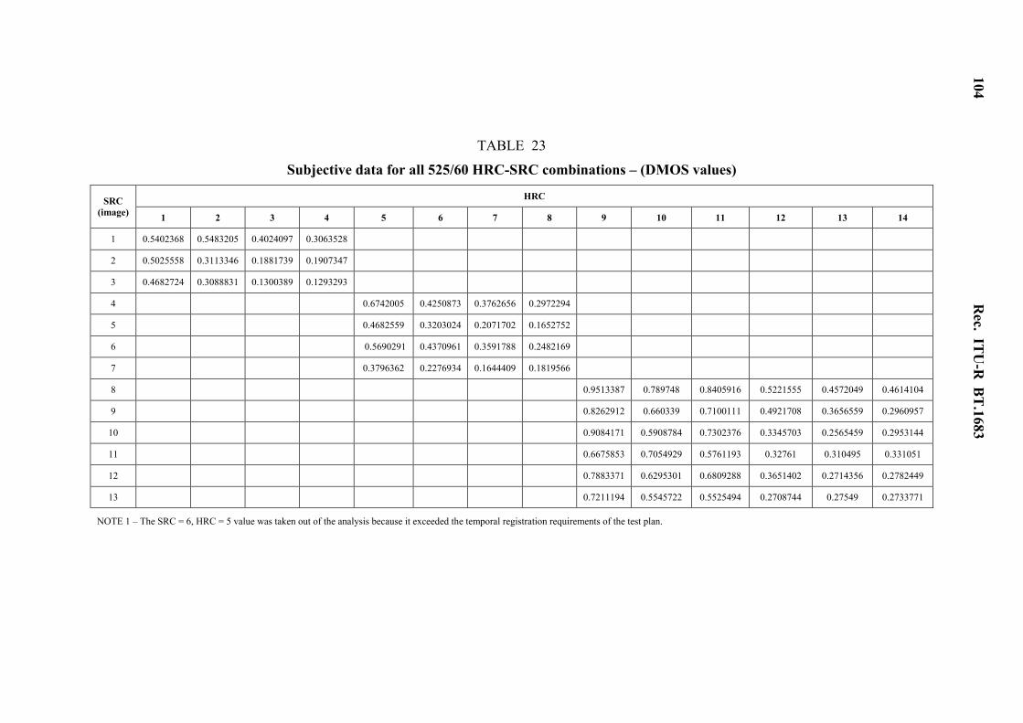
104 R
ec. ITU-R
BT.1683
TABLE 23
Subjective data for all 525/60 HRC-SRC combinations – (DMOS values)
HRC SRC (image) 1 2 3 4 5 6 7 8 9 10 11 12 13 14
1 0.5402368 0.5483205 0.4024097 0.3063528
2 0.5025558 0.3113346 0.1881739 0.1907347
3 0.4682724 0.3088831 0.1300389 0.1293293
4 0.6742005 0.4250873 0.3762656 0.2972294
5 0.4682559 0.3203024 0.2071702 0.1652752
6 0.5690291 0.4370961 0.3591788 0.2482169
7 0.3796362 0.2276934 0.1644409 0.1819566
8 0.9513387 0.789748 0.8405916 0.5221555 0.4572049 0.4614104
9 0.8262912 0.660339 0.7100111 0.4921708 0.3656559 0.2960957
10 0.9084171 0.5908784 0.7302376 0.3345703 0.2565459 0.2953144
11 0.6675853 0.7054929 0.5761193 0.32761 0.310495 0.331051
12 0.7883371 0.6295301 0.6809288 0.3651402 0.2714356 0.2782449
13 0.7211194 0.5545722 0.5525494 0.2708744 0.27549 0.2733771
NOTE 1 – The SRC = 6, HRC = 5 value was taken out of the analysis because it exceeded the temporal registration requirements of the test plan.

Rec. ITU-R BT.1683 105
TABLE 24
Subjective data for all 625/50 HRC-SRC combinations – (DMOS values)
HRC SRC (image) 1 2 3 4 5 6 7 8 9 10
1 0.59461 0.64436 0.40804 0.34109 0.2677 0.26878
2 0.54173 0.70995 0.27443 0.22715 0.21133 0.16647
3 0.73314 0.76167 0.49848 0.38613 0.34574 0.26701
4 0.58528 0.90446 0.62361 0.61143 0.43329 0.26548
5 0.61973 0.68987 0.41648 0.4218 0.27543 0.2022
6 0.38852 0.44457 0.27983 0.28106 0.23726 0.17793
7 0.59953 0.55093 0.45163 0.35617
8 0.32528 0.32727 0.30303 0.26366
9 0.47656 0.49924 0.39101 0.37122
10 0.70492 0.58218 0.49711 0.37854
11 0.79919 0.59256 0.34337 0.30567
12 0.61418 0.6661 0.53242 0.44737
13 0.74225 0.66799 0.42065 0.33381
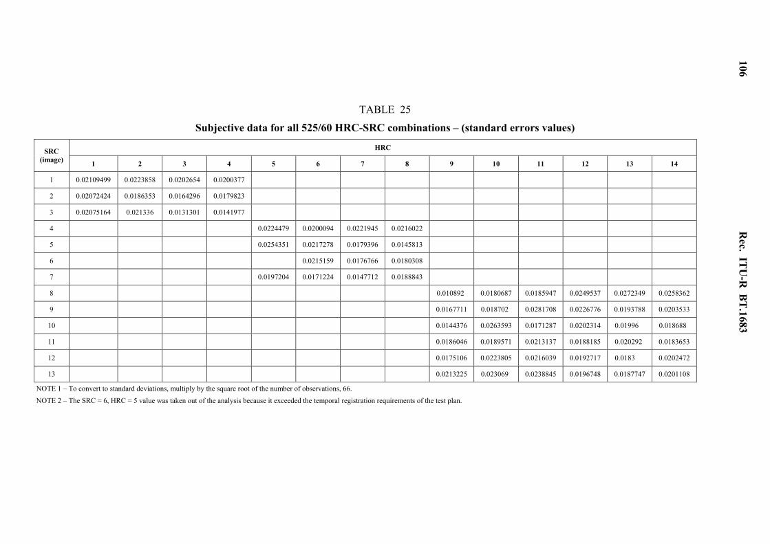
106 R
ec. ITU-R
BT.1683
TABLE 25
Subjective data for all 525/60 HRC-SRC combinations – (standard errors values)
HRC SRC (image) 1 2 3 4 5 6 7 8 9 10 11 12 13 14
1 0.02109499 0.0223858 0.0202654 0.0200377
2 0.02072424 0.0186353 0.0164296 0.0179823
3 0.02075164 0.021336 0.0131301 0.0141977
4 0.0224479 0.0200094 0.0221945 0.0216022
5 0.0254351 0.0217278 0.0179396 0.0145813
6 0.0215159 0.0176766 0.0180308
7 0.0197204 0.0171224 0.0147712 0.0188843
8 0.010892 0.0180687 0.0185947 0.0249537 0.0272349 0.0258362
9 0.0167711 0.018702 0.0281708 0.0226776 0.0193788 0.0203533
10 0.0144376 0.0263593 0.0171287 0.0202314 0.01996 0.018688
11 0.0186046 0.0189571 0.0213137 0.0188185 0.020292 0.0183653
12 0.0175106 0.0223805 0.0216039 0.0192717 0.0183 0.0202472
13 0.0213225 0.023069 0.0238845 0.0196748 0.0187747 0.0201108
NOTE 1 – To convert to standard deviations, multiply by the square root of the number of observations, 66.
NOTE 2 – The SRC = 6, HRC = 5 value was taken out of the analysis because it exceeded the temporal registration requirements of the test plan.

Rec. ITU-R BT.1683 107
TABLE 26
Subjective data for all 625/60 HRC-SRC combinations (standard errors values)
6 References
ATIS [October 2001] Technical Report T1.TR.72-2001 – Methodological Framework for Specifying Accuracy and Cross-Calibration of Video Quality Metrics, Alliance for Telecommunications Industry Solutions, 1200 G Street, NWn Suite 500, Washington DC.
HRC SRC (image) 1 2 3 4 5 6 7 8 9 10
1 0.040255 0.039572 0.038567 0.040432 0.040014 0.036183
2 0.038683 0.033027 0.040957 0.038301 0.042618 0.033956
3 0.039502 0.039111 0.039109 0.042553 0.044151 0.036685
4 0.031762 0.024408 0.036375 0.031371 0.02973 0.042911
5 0.034299 0.044757 0.0407 0.03597 0.033742 0.041272
6 0.040602 0.040035 0.03707 0.043341 0.035289 0.040621
7 0.037894 0.032156 0.038034 0.036946
8 0.036819 0.041563 0.036988 0.037467
9 0.040289 0.040265 0.04015 0.039649
10 0.030283 0.038334 0.037966 0.041339
11 0.034761 0.034838 0.041778 0.041516
12 0.037332 0.036964 0.031253 0.035114
13 0.035205 0.038385 0.038371 0.043687
NOTE 1 – To convert to standard deviations, multiply by the square root of the number of observations, 27.