Embed Size (px)
Citation preview
Recent Great Depressions: Aggregate Growth in New Zealand and Switzerland*
Timothy J. Kehoe
Department of Economics, University of Minnesota, Minneapolis, Minnesota 55455, Research Department, Federal Reserve Bank of Minneapolis, Minneapolis,
Minnesota 55480, and National Bureau of Economic Research, Cambridge, Massachusetts 02138
and
Kim J. Ruhl Stern School of Business, New York University, New York, New York 10012
April 2003 Revised March 2007
*© 2003, Timothy J. Kehoe and Kim J. Ruhl. We have greatly benefited from the discussions surrounding the “Great Depressions: New Zealand and Switzerland in the Late Twentieth Century” workshop at Victoria University of Wellington, February 2002. We are also grateful to seminar participants at the New Zealand Institute of Economic Research and the University of Auckland. We would like to thank Phillip Bishop, Phil Briggs, Stephen Burnell, Brian Easton, Tim Hazledine, Ralph Lattimore, John McDermott, Andrew Philpott, Dennis Rose, and Mark Walton for insightful discussion and valuable references. We also thank two anonymous referees for helpful comments. The data used in this paper are available at http://www.econ.umn.edu/~tkehoe/ and http://www.greatdepressionsbook.com. The views expressed herein are those of the authors and not necessarily those of the Federal Reserve Bank of Minneapolis or the Federal Reserve System.
Abstract Throughout the 1950s and 60s real GDP per working-age person in New Zealand and Switzerland grew at rates at or above the 2 percent trend growth rate of the United States. Between 1973 and 2000, however, real GDP per working-age person in both countries has fallen a cumulative 30 percent below the trend growth path. Our growth accounting attributes almost all of the changes in output growth to changes in the growth of total factor productivity (TFP), and not to changes in labor or capital accumulation. A calibrated dynamic general equilibrium model that takes TFP as exogenous can explain almost the entire decline in relative output in both New Zealand and Switzerland. To understand the recent growth experiences in New Zealand and Switzerland, it is necessary to understand why TFP growth rates have fallen so much. Journal of Economic Literature Classification Codes: E32, N10, O40. Key Words: depression, growth accounting, total factor productivity, dynamic general equilibrium.
1
As measured in the Penn World Tables, Switzerland had the highest income per
capita in the world in 1970, and New Zealand the eighth. By 2000, Switzerland had
fallen to eighth, and New Zealand had tumbled to twenty-second in the rankings.1 These
changes are less an indication of the rapid growth in other countries than they are the lack
of growth in New Zealand and Switzerland. Both New Zealand and Switzerland have
lost about 30 percent of their output per working-age person, vis-à-vis the United States,
over the last 30 years. In this paper, we analyze the growth of these two countries using
the relatively new neoclassical depression methodology, which is based upon the
standard neoclassical growth model.
Our results suggest that movements in total factor productivity (TFP) can largely
explain the poor growth performance in New Zealand and Switzerland. Our growth
accounting attributes almost the entire decline in output to changes in TFP and a
relatively insignificant amount to changes in labor and capital inputs. We calibrate a
simple dynamic general equilibrium model to the two countries and find that a model in
which TFP is exogenous can explain about 96 percent of the decline in output for New
Zealand and more than 100 percent of the decline for Switzerland.
In New Zealand, TFP grew on trend until it fell rapidly between 1974 and 1980,
then leveled out, and now seems to be growing on a lower trend path. This observation is
important in terms of the previous work on New Zealand’s productivity. New Zealand
underwent one of the most radical and complete set of market reforms in the late 1980s,
including labor market reform, foreign trade liberalization, privatization of publicly
owned enterprises, and tax reform.2 The importance of these reforms has focused much
of the research on productivity in New Zealand to the period immediately before and
after the implementation of the reforms. This line of research has been successful in
evaluating the reforms and their effects and has provided valuable insight for policy
makers. Our results suggest, however, that the economy of the 1970s and early 1980s
needs to be more closely studied to understand the current situation.
1 This specific comparison is based on the GDP per adult equivalent series in the Penn World Tables. Switzerland’s GDP per adult equivalent, expressed in Penn World Table constant 1996 international prices was $23,332 – 22 percent larger than the United States, the second richest country in 1970 – and $28,796 in 2000. New Zealand’s GDP per adult equivalent was $16,242 in 1970 and $21,675 in 2000. 2 See Evans, Grimes, Wilkinson, and Teece (1996) for a survey of the reforms and their initial outcomes.
2
Total factor productivity — as a residual after taking the impact of changes in
capital and labor inputs out of changes in real output — includes the effects of a
country’s institutions, such as taxes, openness to foreign competition, and legal system.
Changes in institutions can change the growth path of TFP. The identification of these
changes seems to be the key to understanding aggregate growth in New Zealand. A
frequently cited candidate for the cause of New Zealand’s poor performance is the
decline of its terms of trade. (See, for example, Rose 1985 and Easton 1997, chap. 5.)
The beginning of the great depression in New Zealand coincides with its loss of favored
access to markets in its major trade partner due to the United Kingdom’s accession to the
European Economic Community (EEC). Data show a subsequent sharp fall in the terms
of trade and large changes in New Zealand’s trade patterns. The resulting disruption in
production patterns is a promising candidate for the drop in TFP growth rates.
In Switzerland, TFP fell steadily compared to trend from 1973 to 1996, and this
fall explains most of Switzerland’s great depression. TFP and GDP grew at their
respective trend rates following 1996, but do not appear to be returning to their previous
trend paths. As in New Zealand, that TFP explains almost everything leaves us needing
to explain TFP. In particular, we are left looking for the changing institutional factors
that are reflected in our measurement of TFP. Switzerland’s institutions include highly
protected domestically oriented sectors such as telecommunications, agriculture,
construction, and information technology. These sheltered sectors have had declining
labor productivity, while the sectors exposed to competition have seen improvements.
These facts are especially relevant considering Switzerland’s failure to join the European
Union, a move that would have forced many of these protected sectors to face
international competition and European Union-mandated deregulation. Switzerland did
begin a series of reforms aimed at increasing the competitiveness in these sectors as part
of its revitalization plan, however. These reforms began to be implemented in the late
1990s and seem to coincide with the increased GDP and TFP growth rates found in the
same period.
The next two sections outline the neoclassical depression methodology and its
implementation. First we present the results of our growth accounting, and then we show
how a calibrated growth model can reproduce the observed changes in output. We go on
3
to discuss possible reasons for the decline in TFP for each country and suggests possible
directions for future research on determining the causes of the modern great depressions
in New Zealand and Switzerland.
Neoclassical Depression Methodology
Studying depressions using the neoclassical growth model is a relatively new
methodology. Cole and Ohanian (1999) first applied the growth model to study the Great
Depression of the 1930s in the United States. This successful application led to the study
of depressions around the world using this method, including the depressions in
Argentina (Kydland and Zarazaga 2002), Canada (Amaral and MacGee 2002), Chile and
Mexico (Bergoeing, Kehoe, Kehoe, and Soto 2002), France (Beaudry and Portier 2002),
Germany (Fisher and Hornstein 2002), Italy (Perri and Quadrini 2002), Japan (Hayashi
and Prescott 2002), and the United Kingdom (Cole and Ohanian 2002). For more details
on the methodology, as well as an extensive collection of applications, see Kehoe and
Prescott (2003).
We study a country’s economic growth by measuring its real GDP per working-
age person relative to a trend. We concentrate on GDP per working-age person instead of
the more common per capita measure since it is consistent with our theoretical economy
in which the entire working-age population is capable of working. Because of the
availability of data, we choose to count those aged 15-64 as the working-age population
and, thus, most likely to be available for work. (We compare GDP per working-age
person and GDP per capita in Appendix B.) We work with a Cobb-Douglas specification
of the aggregate technology:
1 ,t t t tY A K Lα α−= (1)
where tY is GDP in year t , tK is the capital stock, tL is hours worked, and tA is TFP.
When TFP grows at a constant rate (that is, when TFP is ( )1 ttA Ag α−= ), the neoclassical
growth model implies a unique balanced growth path in which output and capital per
worker grow at the same constant rate, 1g − . It is relative to this trend growth rate that
we measure a country’s performance.
4
Kehoe and Prescott (2002) argue that this trend growth in TFP represents the
world stock of useable production knowledge growing smoothly over time and that this
knowledge is not country-specific. We define the trend growth rate to be 2 percent per
year, corresponding to the growth rate of GDP per working-age person for the United
States over the period 1920-2000. Kehoe and Prescott (2002) consider the United States
to be the best choice because it is a large, relatively stable country and because it is the
current industrial leader. As shown in Figure 1, the 2 percent trend in GDP per working-
age person fits the U.S. data very well, with the only major deviations from trend being
the Great Depression, 1929-1939, and the World War II buildup, 1939-1946.
The stock of world production knowledge is common across countries, but
countries differ in their institutional structures. This implies that, even though all
countries on a balanced growth path grow at the same rate, each country is on its own
growth path. These paths differ in their levels of output per working-age person.
Countries with institutions that encourage efficiency grow on a path with higher output
per working-age person than countries with institutions that encourage rent seeking or
other activities that lower efficiency. The institutions that determine these paths include
competition policy, bankruptcy systems, and the legal system. The parts of these
institutions that affect neither labor input nor the accumulation of capital are captured in
TFP. Changing institutions changes the path of TFP, moving a country to a new
balanced growth path. One of the central premises of the neoclassical depression
methodology is that explaining movements in TFP involves identifying the changing
institutions.
Figure 2 and Figure 3 display output per working-age person for New Zealand
and Switzerland for 1920-2000. Though our analysis is restricted to the recent great
depressions in New Zealand and Switzerland, the long-term movements in a country
provide interesting perspective. As is shown in Figure 2, New Zealand grew on its 2
percent balanced growth path from about 1938 to 1974, before falling sharply below
trend. The period 1929-1932 is what New Zealand economic historians refer to as “The
Depression” (Hawke 1985). This episode was marked by a sharp drop below trend,
followed by a quick recovery. In contrast, the recent great depression has been slower to
develop, but GDP per working-age person has deviated more from trend, and for a much
5
longer period. In Switzerland, we see a different pattern. Switzerland experienced
almost no growth from 1930 to 1944, which is significantly better than the situation in
other Western European countries, where output fell significantly during the interwar
depression and World War II. As did the rest of Western Europe after World War II,
Switzerland grew faster than trend from 1944 to 1973. The other countries, however,
tended to move to new, higher, balanced growth paths in the 1970s and 1980s. As an
example, in Figure 4 we plot GDP per working-age person for Italy, whose experience is
fairly typical of a number of Western European countries. Italy’s output fell sharply
during World War II, grew faster than trend as Italy recovered from the war, and then
settled into a new growth path in the 1970s. Instead of moving to a new balanced growth
path, as in Italy, Switzerland’s GDP per working-age person grew much slower than
trend following 1973.
Figure 5 and Figure 6 present output per working-age person for New Zealand
and Switzerland over the last half-century. The data are presented with the 2 percent
trend removed, and the series are normalized so that GDP per working-age person is 100
in the first year of the great depression. For New Zealand, the first year of the great
depression is 1974, while in Switzerland the Depression starts a year earlier, in 1973. In
New Zealand, output per working-age person grew on trend from 1955 to 1974 with a
small deviation from trend in the late 1960s. Switzerland, however, was below trend, and
grew faster from 1955 to 1970. This is not unusual, as most of Europe grew faster than
the trend growth rate as it recovered from World War II. What is striking about Figure 5
and Figure 6 is the severe and prolonged decline in trend-adjusted output that the
countries experienced starting in the mid-1970s. New Zealand’s trend-adjusted output
per working-age person fell by 21 percent from 1974 to 1984, and Switzerland’s GDP
declined by 19 percent over the period 1973-1983. In New Zealand, output continued to
fall and was only 67 percent of its trend-corrected 1974 level in 2000, and in Switzerland
output was only 70 percent of its 1973 level in 2000.
It is important to note that Figure 5 and Figure 6 reflect an internal comparison of
output growth. Both New Zealand and Switzerland had relatively high incomes per
capita compared to many other countries in any given year. As measured in the Penn
World Tables, Switzerland had the highest income per capita in the world in 1970 and
6
still had one of the 10 highest incomes per capita in 2000. New Zealand ranked eighth in
1970 and twenty-second out of the 133 countries for which data were available in 2000.
The decline in the cross-sectional ranking is another indicator of these two countries’
poor growth.
Great Depression or Slow Growth?
Some might object to our use of the term “great depression” to describe the
situations in New Zealand and Switzerland. Mention of the Great Depressions in the
United States and the United Kingdom during the interwar years conjures up images of
bread lines and mass unemployment. The people of New Zealand and Switzerland have
not experienced this kind of displacement, nor do outsiders view the countries as being
depressed. Though these deviations from trend have not resulted in massive
displacement or brought international scrutiny and concern, a simple comparison with
Japan places important perspective on the seriousness of the New Zealand and
Switzerland great depressions.
Kehoe and Prescott (2002) consider two characteristics important in defining a
great depression. First, the deviation of output per working-age person from trend must
be large, and second, the deviation from trend must occur quickly. Using the
methodology outlined in the previous section, they define a period of economic growth
below trend as a great depression if it meets the following three conditions:
1. There is no significant recovery during the period in the sense that there is no
subperiod of a decade or longer in which the growth of output per working age person
returns to rates of 2 percent or better.
2. There is at least one year in which output per working-age person is at least 20
percent below trend.
3. There is at least one year in the first decade of the great depression in which output
per working-age person is at least 15 percent below trend.
7
It is clear from Figure 5 and Figure 6 that the economic performances of New Zealand
over the period 1974-2000 and Switzerland over the period 1973-2000 meet these
criteria.
The sizes of New Zealand and Switzerland, as well as their relative importance in
the world economy, have kept much of the international attention away from their poor
growth. To appreciate the importance of this, we only need to look to Japan. Detrended
output per working-age person in Japan has fallen by about 9 percent over the period
1991-2002 and continues to fall.3 Figure 7 displays detrended output per working-age
person for Japan. When we compare Figure 7 to Figure 5 and to Figure 6, it is obvious
that the current depression in Japan is milder than were the first decades of the
depressions in New Zealand and Switzerland. Japan’s importance in the world economy,
however, has attracted attention to its situation. The 16 February 2002 cover of The
Economist reads “The Sadness of Japan” and features a special report on Japan’s troubled
economy. Two weeks later, the 3 March 2002 issue of The Economist reports that “by
several measures, Japan’s slump is now worse than America’s was in the 1930s.”
Japan’s economy may be headed into a great depression. Economists, policy
makers, and observers agree that the lack of economic growth in Japan is a serious
concern. If New Zealand and Switzerland were as large as Japan, their situations might
be as widely publicized and fretted over. People know that Japan is in trouble, and not
just experiencing slow growth. Compared to Japan, the periods 1974-2000 in New
Zealand and 1973-2000 in Switzerland were worse and were, indeed, great depressions.
Whether or not these countries are still in great depressions remains to be seen.
From 1992 to 2002, New Zealand managed to grow at or above the trend growth rate. If
growth continues to beat the trend rate, New Zealand may be returning to its previous
balanced growth path. We cannot rule out, however, the possibility that New Zealand
may continue to grow at about 2 percent per year and is settling into a new, lower
balanced growth path. For Switzerland, the return to the trend growth rate appears to
happen in about 1996. From 1996 to 2000, GDP per working-age person grew at a little
3 It should be noted that, because of the rapid aging of Japan’s population, it makes a difference how we define working age. If we define working age as 20-69 years, for example, the drop in real GDP per working-age person between 1991 and 2002 was about 14 percent. The age structures of the populations of New Zealand and Switzerland are more stable than that of Japan. This point is addressed in Appendix B.
8
less than 2 percent per year on average. Again, it could be Switzerland settling into a
new, lower balanced growth path. We simply do not have enough data, however, to
determine whether or not these countries are continuing onto lower balanced growth
paths. Only time can answer this question, and we focus our attention on the period 1974-
1992 for New Zealand and 1973-1996 for Switzerland, periods in which we know the
two countries were in great depressions.
Growth Accounting
To evaluate the contributions of various factors to the changes in output per
working-age person, we set up an accounting framework based on the neoclassical
growth model. For a more detailed discussion of the foundations and motivation for the
particular functional forms and a thorough analysis, see Kehoe and Prescott (2002) and
Prescott (2002).
As explained earlier, we model aggregate production using the Cobb-Douglas
form. Since we are concerned with growth in output per working-age person relative to a
balanced growth path, it is useful to write the production function in terms of output per
working-age person and measures of factor inputs that are constant along a balanced
growth path:
1
11 ,t t tt
t t t
Y K LAN Y N
αα
α
−
−⎛ ⎞
= ⎜ ⎟⎝ ⎠
(2)
where tY is output, tK is capital, tL is labor, tN is working-age population, and tA is
TFP. TFP is calculated as the residual after accounting for capital and labor:
1 .t t t tA Y K Lα α−= (3)
To compute the tA series for New Zealand and Switzerland, we compile data on output,
labor, and investment from each country’s national accounts. Labor is measured as total
hours worked. We construct tL by multiplying the country’s average yearly employment
by the average number of hours worked per week. Using investment data, we generate
the series of capital stocks using
( )1 1 ,t t tK K Xδ+ = − + (4)
9
where tX is investment (measured as changes in inventories and gross fixed capital
formation) and δ is the depreciation rate. Given a value for δ , we choose the initial
capital stock so that the capital-output ratio is the same in 1954 as its average over the
period 1954-1970. We set 0.056δ = , which implies that capital consumption as a
fraction of output, t tK Yδ , is 0.167 for Switzerland in 1970, the same as the capital
consumption allowance as a share of GDP that is reported in the Swiss national accounts.
For New Zealand, this value of δ implies a capital consumption ratio of 0.146 in 1970,
while in the data it is 0.090. A value of δ less than 0.03 is needed to match the capital
consumption ratio for New Zealand. We choose to use 0.056 since the lower value of δ
seems implausibly small compared to the values for comparable countries.
We still need to choose a value for capital’s share of income, α . Unfortunately,
neither New Zealand nor Switzerland publishes data detailed enough to compute labor
and capital shares as in Cooley and Prescott (1995) or in Gollin (2002). These methods
require, at a minimum, information on the operating surplus of private unincorporated
enterprises. When we compute the crude labor share of income ( )1 α− that does not
account for the self-employed, we find values that imply α around 0.44 and 0.34 for
New Zealand and Switzerland, respectively.4 Gollin (2002) shows that factor shares
adjusted for self-employment income and sectoral composition are remarkably constant
across both time and countries, however, and that the capital shares cluster around 0.30.
Given the evidence presented in Gollin (2002) and our crude calculation of factor shares,
we choose to set capital’s share of income,α , to 0.300 for both countries.5 Results of
numerical experiments not reported here show that our qualitative conclusions are not
very sensitive to the values that we have chosen for α and δ .
Using the series for labor, output, and the constructed capital stocks, we compute
TFP for each of the countries. In the balanced growth path, hours worked per working-
age person are constant, and output and capital both grow at the same constant rate. It is
then easy to see from (2) that in a balanced growth path in which output per working-age
4 The crude method is simply 1 α− = compensation of employees / (GDP-net indirect taxes). 5 It may be the case that returns to land are more important in New Zealand than they are in countries like the United States, and that this accounts for the low measured depreciation and the low measured labor share. This is a topic that merits further study.
10
person grows at 2 percent per year, the TFP component of output, 1 1tA α− , must also grow
at 2 percent per year. Thus, we detrend the TFP component by 2 percent per year.
Throughout this section and the next, we concentrate on the TFP component, 1 1tA α− , but it
should not be confused with the level of TFP, tA .
Figure 8 and Figure 9 plot GDP per working-age person and the TFP component
for New Zealand and Switzerland. A striking feature of both figures is the similarity of
the TFP component and GDP per working-age person. In fact, the simple correlation
coefficient for the TFP component and GDP per working-age person over the period
1970-2000 is 0.93 for New Zealand and 0.99 for Switzerland. This simple statistic
suggests that TFP has played an important role in determining the growth in output in
these countries.
To quantify the contributions of the TFP component and other factors in the
growth of these two economies, we use our theoretical framework to guide our growth
accounting. As in Hayashi and Prescott (2002), we can take logarithms of the production
function (1) and rearrange terms to relate output per working-age person, hours worked
per working-age person, the TFP component, and the capital-output ratio:
( )1log log log log .1 1
t t tt
t t t
Y K LAN Y N
αα α
⎛ ⎞ ⎛ ⎞ ⎛ ⎞= + +⎜ ⎟ ⎜ ⎟ ⎜ ⎟− −⎝ ⎠ ⎝ ⎠ ⎝ ⎠
(5)
This expression can be used to decompose the average annual growth rate of output per
working-age person over a number of years, s , into
( ) ( ) ( ) ( )
( ) ( ) ( ) ( )
log log log log11
log log log log.
1
t s t s t t t s t
t s t s t t t s t s t t
Y N Y N A As s
K Y K Y L N L Ns s
α
αα
+ + +
+ + + +
⎡ ⎤− −= ⎢ ⎥− ⎣ ⎦
⎡ ⎤ ⎡ ⎤− −+ +⎢ ⎥ ⎢ ⎥− ⎣ ⎦ ⎣ ⎦
(6)
The above expression decomposes changes in output per working-age person into
changes in the TFP component (the first term on the right-hand side), changes in the
capital-output ratio (the second term on the right-hand side), and changes in hours
worked per working-age person (the last term on the right-hand side). Along the
balanced growth path, both hours per worker and the capital-output ratio are constant, so
11
we would expect these terms in (6) to be very small in our growth accounting if the
economy is on the balanced growth path.
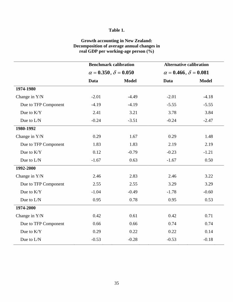
We present the results of this decomposition for New Zealand in the first column
of Table 1. In the period 1974-1980, output per working-age person declined by 2.01
percent per year. 6 The TFP component fell by 3.68 percent per year over this period, but
was offset by the capital-output ratio, which grew at 1.91 percent. From 1980 to 1992,
GDP growth was well below the trend growth rate, averaging only 0.29 percent per year.
Over this same period, the TFP component grew near its trend growth rate, averaging
1.91 percent per year. Large declines in labor input over this period contributed to the
low GDP growth, however. From 1992 on, both the TFP component and GDP per
working-age person grew at rates slightly above their trend growth rates. In this period,
labor grew substantially, mostly offsetting the decreases from the earlier period.
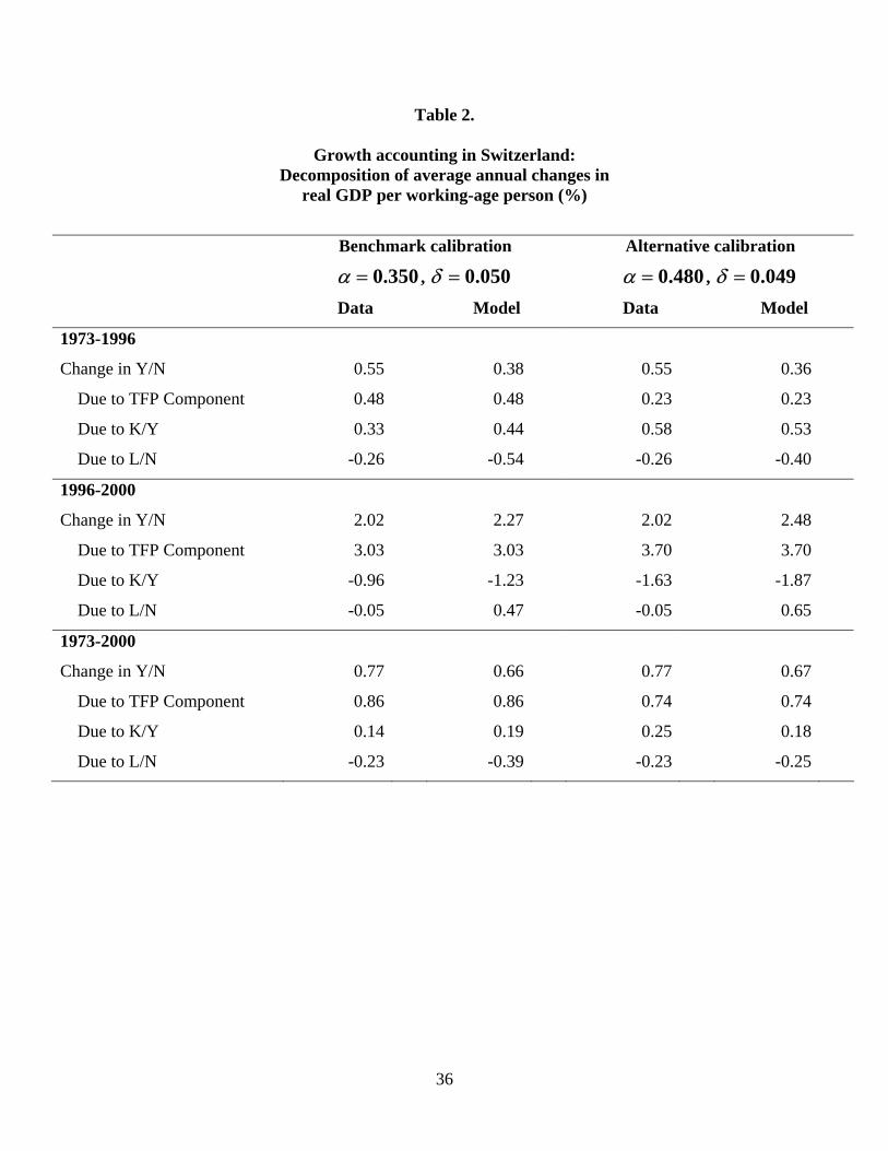
The growth accounting for Switzerland, shown in Table 2, attributes even more of
the change in GDP per working-age person to the TFP component. In the period 1973-
1996, output per working-age person grew at only 0.44 percent per year, and changes in
the TFP component accounted for most of this, increasing by 0.47 percent per year over
the same period. In this period there were only small movements in the labor input and
the capital-output ratio. As has New Zealand, Switzerland has managed to increase its
growth recently. Over the period 1996-2000, GDP per working-age person has grown at
approximately 1.79 percent per year, which is mostly accounted for by a 2.67 percent
growth rate in the TFP component. In this period the capital-output ratio’s contribution
to output growth was negative, as in New Zealand, and labor input was roughly constant.
The growth accounting confirms our intuition gained from the plots of the TFP
component and output. Output growth in New Zealand and Switzerland seems to be
largely accounted for by changes in the TFP component. The contributions of labor and
capital are not trivial, however, particularly the contributions of labor in New Zealand. In
the next section we construct a model to explore the extent to which exogenous
productivity changes can account for the findings of this section.
6 The growth rates can be expressed as approximately percentage growth rates because the difference in log values will approximate percentage changes for small changes in the variables. The decomposition in (6) has the advantage of being additive.
12
Baseline Model
We calibrate a simple dynamic general equilibrium model to see how much of the
change in output we can account for using only productivity changes. In this model
agents live in a closed economy and have perfect foresight over the sequence of
productivity. The model features a representative agent who maximizes the utility
function
( ) ( ) ( )1970log 1 logt
t t ttC hN Lβ γ γ∞
=⎡ ⎤+ − −⎣ ⎦∑ (7)
subject to a sequence of budget constraints,
( )1 1 ,t t t t t tC K w L r Kδ++ = + + − (8)
and has an initial stock of capital, 1970K . The total number of hours available for work is
thN , where tN is the working-age population and h is the number of hours available for
market work per week. We choose h to be 100. To be consistent with our growth
accounting, the production technology in the economy is of the Cobb-Douglas form,
implying the following feasibility constraint:
( )11 1 .t t t t t tC K A K L Kα α δ−++ = + − (9)
The utility function’s parameters β and γ must be calibrated before solving the
model. From the producer’s problem, we have the standard expressions for wages and
capital rental rates,
( ) 1 11 ,t t t t t t t tw A K L r A K Lα α α αα α− − −= − = (10)
which allows us to use the consumer’s first-order conditions to compute β and γ as
( )1 1
t
t t
CC r
βδ+
=+ −
(11)
( )
,t
t t t t
CC w hN L
γ =+ −
(12)
where 0.300α = and 0.056δ = as in our growth accounting. We use data on
consumption, capital, hours worked, and working-age population from 1954 to 1970 to
compute values for β and γ for each year. We then take averages over this period and
13
obtain 0.979β = and 0.259γ = for New Zealand and 0.989β = and 0.364γ = for
Switzerland. It is worth pointing out that the high calibrated value of γ for Switzerland
compared to that for New Zealand reflects the fact that the average working-age person in
Switzerland worked much more over the period 1954-1970 than did the average working-
age person in New Zealand. As Lambelet and Mihailov (2000) stress, the level of hours
worked per working-age person is high in Switzerland compared to its levels in many
other industrialized countries.
It should be pointed out that the real investment series used to calculate the capital
stock in (4) and to calibrate the discount factor β using the consumption-investment
trade-off in (11) is formed by deflating nominal investment by the GDP deflator rather
than by the investment deflator. This decision makes a lot of sense when we are thinking
in terms of the labor leisure trade-off (11). It makes less sense when we are thinking in
terms of capital accumulation (4). An alternative formulation worth exploring would
replace the feasibility condition (9) with
( )1 1 .t t t t t t tC q X A K L Kα α δ−+ = + − (13)
( )1 1t t tK K Xδ+ = − + . (14)
Here tq is the price of the investment good, measured as the ratio of the invest deflator to
a deflator for the rest of GDP. In this framework some of technological progress shows
up in increases in TFP and some in a fall in the relative price of investment.
Given the values for the parameters, the initial capital stock, and series for tN and
tA , we solve the model for New Zealand and Switzerland over 1970-2009. For 1970-
2000 the values of tA and tN are exactly those from the data, and we set the initial
capital stock to its 1970 value. For 2001-2009, we assume TFP grows at the same
average rate at which it grew from 1954 to 1970 and that the population grows at the
same rate it did between 1999 and 2000. We impose the terminal condition that the
equilibrium of the model converge to a balanced growth path by 2009.
Figure 10 and Figure 11 display the results of numerical experiments of the model
for New Zealand and Switzerland. For both New Zealand and Switzerland, the model
does a good job of accounting for the falling output per working-age person. For New
14
Zealand, detrended output per working-age person fell by 36 percent from 1974 to 1992,
while the model’s output falls 33 percent over the same period. The model captures the
changes in the capital-output ratio as well. The model does not generate the large change
in labor we see in the late 1980s and early 1990s. Beginning in 1987, the number of
hours worked per week per working-age person decreased steadily from 24 to 20 in 1991.
Following 1991, hours worked increased sharply and have remained between 22 and 23
hours per week. These movements in hours worked are most likely the result of the
extensive labor market and welfare reforms that were implemented throughout the early
1990s. Our model does not take these large policy changes into account.
The model reproduces the features of the Swiss data well. The model’s output per
working-age person falls by 32 percent from 1973 to 1996, compared with 30 percent in
the data. The model also does an impressive job of tracking the capital-output ratio.
Changes in the model’s hours-worked series also match the data fairly well, although the
levels are too high, and this accounts for most of the deviations between the model’s
GDP from that in the data. Over the period 1970-2000, working-age persons in
Switzerland have worked fewer hours than they had done during the period 1954-1970 to
which we have calibrated the parameter γ that is crucial in governing the labor-leisure
trade-off.
In the second columns of Table 1 and Table 2 we display the results of our growth
accounting on the model’s labor, capital, and output series. A comparison of the first and
second columns in Table 1 confirms the model’s ability to generate the features of the
New Zealand data. The differences between the model results and the data are largely
accounted for by differences in labor input: the data have a smaller drop in hours worked
over the period 1974-1980 than does the model, but the data have another drop, rather
than a small increase, over 1980-1992. Growth accounting in the Swiss model is even
more striking. A simple growth model augmented with TFP shocks not only captures the
changes in output, but also does a good job of matching the contributions of labor and
capital to output growth.
15
Explaining TFP
Our growth accounting makes it clear that understanding the economic
performance of New Zealand and Switzerland requires an understanding of TFP. In
attempting to account for cross-country levels of income per capita, Prescott (1998)
concludes that only TFP, and not the accumulation of capital or the labor input, can
account for these differences. Thus, to explain both the cross-country distribution of per
capita income and the large movements of GDP within a specific country, we need to be
able to explain TFP. Prescott (1998) calls for a theory of TFP and suggests that a
candidate theory might involve a country’s resistance to the adoption of more efficient
technologies. This theory is further developed in Parente and Prescott (2002), in which
monopoly rights to work practices are considered as an institution that slows the adoption
of new technologies.
While there is no broadly accepted theory of TFP, a country’s institutions likely
play a large role in the evolution of its TFP. Institutions that may be important include a
country’s openness to foreign competition, the existence of monopoly rights, the
prevalence of labor unions, government regulation of industry, and price controls, among
others. In this section we discuss some of the institutions in New Zealand and
Switzerland that are worth investigating. In particular, we are searching for changes in
the institutional structure in these countries that took place around the beginning of their
depressions and have persisted throughout the period. Temporary “shocks” will not be
able to account for the prolonged depressions, since neither of these countries has
recovered to its trend TFP and output levels.
New Zealand
Given New Zealand’s poor economic performance after 1974, it should come as
no surprise that other researchers have studied the determinants of economic growth
there. Hall (1996) does aggregate growth accounting for New Zealand based on detailed
sectoral calculations by Philpott (1993, 1994). Like us, he finds that TFP is the dominant
source of fluctuations in real GDP. A number of researchers focus on the role of
government intervention in determining productivity. (See Dalziel and Lattimore 2001
and Silverstone, Lattimore, and Bollard 1996.) During the period 1978-1984 the
16
government made large investments, later judged to have been unproductive, as part of
the “Think Big” strategy. The period 1984-1992 was characterized by massive economic
reforms, which have been characterized by some as ill sequenced.
Foreign Trade
Here we consider the effects of external shocks on the New Zealand economy.
New Zealand’s trade (imports plus exports) as a percentage of GDP averaged 56 percent
for the period 1972-1980, larger than that in Australia, the United Kingdom, and Canada.
Since New Zealand is a small open economy, changes in the terms of trade or in trade
policy from outside the country can have significant effects and are frequently cited as a
determinant of growth in New Zealand. As Briggs (2003) stresses, New Zealand’s
foreign trade has grown much more slowly since 1970 than has trade in the rest of the
industrialized world.
We choose to define the terms of trade as the price of a country’s exports relative
to the price of the country’s imports. Easterly, Kremer, Pritchet, and Summers (1993)
present evidence that terms-of-trade shocks can explain a substantial amount of the
variance in GDP growth rates in time series regressions. Working in the same
neoclassical methodology as this study, Perri and Quadrini (2002) attribute a large
portion of Italy’s depression in the 1930s to a combination of increasing trade barriers
and rigid wages. Grimes (1991) finds that the reduction in New Zealand’s terms of trade
over the period 1950-1985 was responsible for a reduction in the annual GDP growth rate
of 0.13 percent.
Our measure of the terms of trade is constructed using the implicit price deflator
for exports and imports from the national accounts. Assume that the prevailing ratio of
the world price for the goods that New Zealand exports to the price of the goods that New
Zealand imports is tp and that the rest of the world levies an ad valorem tariff of *tτ on
New Zealand’s exports. Arbitrage implies that the price received by New Zealand
exporters for their goods is /(1 *)t tp τ+ . Since the implicit price deflator for New
Zealand imports measures market prices it includes any tariffs paid on imports. Let tτ be
the ad valorem tariff on imports into New Zealand. Consequently, our measure of the
terms of trade can be written
17
(1 )(1 *)
tt
t t
pToTτ τ
=+ +
(15)
We plot New Zealand’s terms of trade in Figure 12. New Zealand’s terms of trade level
falls to 85 percent of its 1974 level in 1975 and stays low until 1985, when it starts to
return roughly to its pre 1974 average. It is significant that the sharp drop in New
Zealand’s terms of trade coincided with both the beginning of New Zealand’s great
depression and the accession of the United Kingdom to the EEC. It is, of course, true that
that sharp drop in New Zealand’s terms of trade from 1973 to 1975 coincided with the
first oil shock, but much of the persistence of the terms of trade movements after 1970
can be explained by trade policy. The improvements in the terms of trade in the late
1980s, for example, coincided with significant trade liberalization (Evans et al. 1996).
Following Belich (1996, 2001) we can divide New Zealand’s recent trade history
into two periods, recolonization and decolonization. Recolonization describes the period
1880-1970, in which the trade between New Zealand and the United Kingdom closely
resembled that of a colony providing primary materials to its mother country. As a
colonial farm, New Zealand’s trade relations in this period were characterized by
preferential trade arrangements between the United Kingdom and the Dominions. This
relationship was key to New Zealand’s economy. New Zealand exported wool, dairy,
and pastoral products to the United Kingdom and imported manufactures, fuels, and
capital goods. The bulk purchase agreements between the United Kingdom and New
Zealand guaranteed a market for New Zealand exports during and following World War
II, and restrictions on imports of other products into the United Kingdom further
protected New Zealand’s trade.
Decolonization began in 1970 and continues today, as New Zealand competes in a
world market without preferential U.K. relations. The 1960s ushered in a new era of
New Zealand-United Kingdom trade policy. Beginning in 1960, New Zealand lowered
the preference on U.K. imports and continued to do so until the U.K tariff preference was
phased out in 1977 (Lattimore and Wooding 1996). These changes were partially in
response to the more drastic changes in policy being undertaken in the United Kingdom.
In 1968, the EEC implemented a customs union that eliminated duties between member
countries, and imposed a common external tariff. Five years later, New Zealand’s largest
18
and most accessible trading partner erected major trading barriers when the United
Kingdom joined the EEC in 1973. Though New Zealand retained some special access
under bilateral agreements with the EEC, this change in policy led to a drastic change in
New Zealand’s trading pattern. New Zealand’s external trade was further jeopardized by
the EEC in third markets. New Zealand’s agricultural products now had to compete with
the heavily subsidized agricultural exports of Europe. Even in the United Kingdom,
where New Zealand still enjoyed some privilege, exporters now had to compete with
subsidized U.K. farmers (Hawke and Lattimore 1999).
Evidence of the impact of these barriers is visible in Figure 13 and Figure 14.
Figure 13 shows the share of New Zealand’s total exports and imports sourced from the
United Kingdom. The figure shows the dramatic decline in the United Kingdom’s share
of New Zealand’s imports and exports throughout the 1960s and 1970s. Even though this
share falls throughout the 1960s, there is a sharp decrease from 1972 to 1974 as New
Zealand dealt with the increased trade barriers. Figure 14 reveals an important detail of
this trade pattern. New Zealand sourced more than half of its imported machinery and
transport goods from the United Kingdom in 1965, compared to approximately 4 percent
in 2000.
The changes in New Zealand’s trade patterns are certainly not entirely driven by
the EEC customs union. New Zealand’s protection policies were complex and changing
throughout the pre-reform era. Besides tariffs, the New Zealand government used import
licensing, export incentives, and exchange controls to protect local industry and stimulate
growth. Growth and development in Asia is also likely to have had a strong effect on
New Zealand’s trade patterns. Goods from Asia have replaced the imported capital
goods previously sourced from Europe almost percent-for-percent. It is unlikely,
however, that New Zealand faced trade policies in Asia that were as accommodating as
those from the pre-EEC United Kingdom.
The changes in the terms of trade and the changes in New Zealand’s relationships
with its trade partners — and the resulting disruption in trade patterns — undoubtedly
had a major impact on the New Zealand economy. The results of our numerical
experiments in the previous section indicate that, to assign significant blame to these
external shocks as a cause of New Zealand’s great depression, we need to be able to
19
construct a model in which the impact of these shocks show up in measured TFP. An
obvious direction to take in modeling the impact of changes in the terms of trade and
trade policy would be to model imported goods as intermediates in production as done by
Amaral and MacGee (2002) and Perri and Quadrini (2002). A sharp drop in the terms of
trade and/or an increase in trade barriers can lead to a large decrease in consumption and
investment. As stressed by Kohli (2000), however, this sort of shock will have a much
smaller effect on real GDP because imports are deflated by an import price deflator and
then subtracted from consumption, investment, government spending, and exports to
form real GDP. Consequently, the simple approach that has trade shocks affecting
production by making foreign inputs more expensive cannot account for a large drop in
TFP because it has little effect on measured GDP unless labor and capital inputs change.
An alternative approach would be to model the frictions involved in moving labor and
capital between the sectors that produce exportable goods and nontradable goods into the
sector that produce importable goods as in Kehoe and Fernandez de Cordoba (2000).
A challenge to any theory of New Zealand’s great depression based on trade
shocks is the observation that the return of the terms of trade to higher levels and the
trade liberalization of the late 1980s and early 1990s has not, at least so far, resulted in a
return of New Zealand to its pre 1974 balanced growth path.
Switzerland
None of Switzerland’s falling TFP can be explained by changes in the terms of
trade. As shown in Figure 15, Switzerland’s terms of trade have been steadily increasing
over the last 30 years. Switzerland’s trade patterns have stayed relatively constant over
the last 30 years, indicating that there was probably not any large change in trade
relations. Given the lack of evidence that Switzerland’s external trade has changed
drastically, we turn our attention to two other possible explanations.
Structural Rigidities
Hviding (1998) divides Switzerland’s economy into two sectors, the open sector
and the sheltered sector. The open sector consists of industries that compete in
international markets and are not protected by Swiss trade policy. These industries
20
include most of manufacturing. The sheltered sector is made up of the heavily protected
and subsidized agricultural sector and many of the service industries such as
telecommunications, information technology, and construction.
The sheltered sector’s domestically oriented industries are relatively rigid, and
price-fixing, market-share agreements, and explicit cartels are common. Swiss industries
also enjoy a domestic market segmented by canton-specific technological standards and
licensing. These rigidities may have had less of an impact on aggregate technological
growth in the past, but may be coming to center stage as these protected industries
experience massive technological change.
Hviding (1998) suggests that the combination of structural rigidities and sector-
specific technological change has acted as a drag on Switzerland’s output growth. In the
1950s and 1960s, much of the worldwide innovation took place in the manufacturing
industries. In Switzerland, these sectors faced international competition and needed to
adopt the improving technologies and work practices to stay competitive. From the
1970s onward, however, the important worldwide innovations were concentrated in
sectors such as telecommunications, information technology, and biotechnology. In
Switzerland these industries are part of the sheltered sector. The lack of competition in
these sectors may slow the rate of adoption of more efficient technologies, thereby
slowing aggregate productivity growth.
An analysis of the productivity of these two sectors would allow us to carefully
evaluate this potential explanation for Switzerland’s poor aggregate productivity growth.
Unfortunately, we have been unable to obtain detailed data by industry, particularly data
on capital, for Switzerland. Faced with this constraint, Hviding (1998) assigns
manufacturing to the open sector and the nonmanufacturing private sector to the sheltered
sector. Given this dichotomy, Hviding looks to labor productivity for evidence of slow
productivity growth. Over the period 1965-1975, the Swiss manufacturing sector’s labor
productivity grew at an average annual rate of 2.75 percent. In this same period, the
nonmanufacturing sector’s labor productivity grew at 2.5 percent per year on average. In
the period 1976-1996, manufacturing productivity continued its growth, averaging 2.5
percent per year on average. Nonmanufacturing productivity growth fell to only 0.5
percent per year during the period 1976-1996, however.
21
The combination of structural rigidities and sector-specific technological change
appears to be a plausible explanation for Switzerland’s poor productivity growth. This
preliminary evidence suggests that a detailed analysis of the structure of Swiss industry
might yield important insights into Switzerland’s great depression.
Foreign Labor
A second possible explanation for Switzerland’s poor productivity growth may be
the structure of its work force. Since the early 1970s there has been an increasing stock of
permanent foreign workers in Switzerland. These workers tend to be low skilled, and,
between 1977 and 2000, they have more than doubled their share in unemployment. If
new technology and high-skilled workers are complements, then access to a large pool of
low-skilled workers may hinder the new technology’s adoption.
Sheldon (2000) finds that technological change in Switzerland is skill biased and
that the increasing number of low-skilled, permanent foreign workers is slowing
technological change. Switzerland’s foreign worker policy allows three kinds of
temporary foreign work permits and a permanent permit that entitles the holder to the
same rights as national workers. In particular, permanent permit holders may continue to
live in Switzerland even when they are not employed. Since the 1960s, the fraction of
foreign workers under permanent permits has increased steadily, more than doubling
from 1970 to 2000. Sheldon (2001) reports that the share of permanent and annual
workers in the total workforce has remained relatively constant at about 18 percent, but
that the share of these workers in unemployment has increased from about 20 percent of
unemployment in 1977 to more than 45 percent in 1999.
Sheldon (2000) estimates a trans-log production function for Switzerland, using a
panel of 21 industries and 5 types of labor input. The panel data allow Sheldon to
classify the foreign workers by their permit type. The estimations imply that
Switzerland’s technological change is factor saving with regard to most types of foreign
workers. Sheldon (2001) couples this finding with the rising number of available low-
skilled workers and suggests that firms may be substituting low-wage workers for new
technologies.
22
The lack of productivity growth in the sheltered sector could certainly be related
to the foreign worker situation. The protected sector in Switzerland encompasses many
industries that are considered large employers of low-skilled labor. These industries
include agriculture, restaurants, hotels, and other service industries. The combination of
a relatively uncompetitive environment and a large supply of low-skilled workers may be
important in explaining the recent performance of the Swiss economy.
Quality of Data
Recent work by Abrahamsen, Aeppli, Atukeren, Graff, Müller, and Schips (2003)
argue that our finding that Switzerland has gone though a great depression is partially the
result of the poor quality of Swiss data and that, given this problem with the data, it is
difficult or impossible to compare Swiss economic performance with that of other
countries, like the United States. To start with, Abrahamsen et al. (2003) ignore Swiss
data for the period before 1980 presumably because they feel that these data are so bad
that they have to be discarded completely.7 Notice that, in Figure 6, the period 1973-
1980 was the period of the sharpest drop in GDP per working-age person in Switzerland.
Abrahamsen et al. (2003) then turn to post-1980 data and point out that, in measuring
GDP, the United States uses the System of National Accounts of 1993 (SNA93), while
Switzerland uses the System of National Account of 1968 (SNA68). The SNA93
includes a sector for investment in “intangibles” that is not found in SNA68 and includes
the purchases of software. If either the rate of investment in intangibles increased or the
price of intangibles relative to other goods decreased, then the SNA68-measured GDP
would be lower than the SNA93-measured GDP, conceivably by as much as 5 percent
over the period 1973-2000. We discuss this point further in Appendix B. We should
bear in mind, however, that Hviding (1998) identifies information technology and
telecommunications as sheltered sectors, implying that the adjustment in growth in
moving to SNA93 is likely to be far smaller in Switzerland than it was in the United
States. In any case, Switzerland will adopt Europe’s equivalent to the SNA93, the
7 At least this was the argument presented by Yngve Abrahamsen at the “Great Depressions: New Zealand and Switzerland in the Late Twentieth Century” workshop at Victoria University of Wellington in February 2003.
23
European System of Accounts of 1995, at the end of 2003. The release of this data
should help us to better evaluate the importance of this factor.
Given the arguments of Abrahamsen et al. (2003), we need to maintain some
skepticism in working with Swiss data. Simply giving up on the data, however, would
leave us unable to analyze the causes of the Swiss great depression.
Abrahamsen et al. (2003) also disagree with our concept of national income and
depressions. Instead of using GDP per working-age population, they use output per hour
worked. When we compute GDP per hour worked in Switzerland over the entire period
1973-2000, we find that GDP per hour worked in Switzerland falls by only 14 percent
compared to that in the United States, while GDP per working-age person falls by 32
percent compared to that in the United States. This relative equality of labor
productivity, Abrahamsen et al. (2003) claim, is an indication that Switzerland is not a
depressed country. Thus, they are implicitly defining a depression as a period in which
labor productivity does not grow as fast as labor productivity in the United States.
Because their definition of depression would rule out periods in which drops in output are
driven by massive increases in unemployment, it would probably be best for them to use
another term.
Abrahamsen et al. (2003) also look for evidence of depressions using a measure
much more closely related to ours. They choose to run a regression with cross-country
fixed effects to study the determinants of New Zealand’s and Switzerland’s growth. In
particular, they estimate equations of the form
( ) ( ) ( ) ( ) ,, , , , i i ti t i t i t i tg Y L g A g K L H Lα γ β ε= + + + + , (16)
where g is the growth rate function, Y is output, A is TFP, K is capital, H is human
capital, and L is labor for country i in year t . The country dummy, iβ , captures any
country-specific, time-invariant growth rate differences. The authors choose the
following to serve as a proxy for TFP growth:
( ) ( ) ( )0 1 , 1 2, , 1 , 1log logi ti t US t i t
g A a a T a Y L Y L− − −⎡ ⎤= + + −⎣ ⎦ , (17)
where T is a measure of the stock of knowledge relevant for improving TFP and
( ) ( )log logUS i
Y L Y L− is the development gap to the frontier country. The stock of
technical knowledge, T , is measured by the fraction of the labor force that has completed
24
some form of higher education. Human capital is measured as the mean number of years
of schooling, and labor is measured by the number of people aged 15-64. After
estimating the model, the authors find that the country dummy variables for New Zealand
and Switzerland are not statistically different from zero. They interpret this result as
evidence that there are no depressions in these countries and that no “‘slow growth
puzzle’ remains.” This result squares up well with our theory-based identity that
movements in output per working-age person can be attributed to changes in labor and
capital inputs and to changes in TFP. Notice that, if ( )g A perfectly measured TFP as in
(3), the relationship in (16) would also be an identity, and not only the country fixed
effects iβ , but also the error terms ,i tε would disappear.
Given that movements in inputs and TFP can explain output growth, Abrahamsen
et al. (2003) ask, as do we, What explains these movements in inputs and TFP? Their
answer is that Swiss consumer preferences, particularly over the labor-leisure trade-off,
have changed over time in ways that they have not in countries like the United States. It
is worth stressing that this point of view is drastically at odds with that taken in this
paper. Our point of view is that, while individuals differ in their tastes, people are the
same on average, and the institutions that these people face lead to different outcomes.
For example, the French devote about 30 percent less time to market activities than do
Americans. Does this mean they derive more utility from leisure than do their
biologically identical counterparts across the Atlantic Ocean? Rather than assume away
the difference in hours worked by appealing to differences in preferences, Prescott (2002)
shows that almost all of this difference can be attributed to differences in the two
countries’ tax systems, and not to different preferences.
In this paper, we have estimated different parameters β and γ for New Zealand
and Switzerland for the period 1954-1970, which we use to analyze the economic
performances of these countries over the later period 1970-2000. Our stance is that the
differences in these parameters across the two countries are due to differences in
institutions, like labor market policies. Differences in institutions across the two
countries are relatively unimportant from the perspective of this paper: we are not trying
to answer the question of why Switzerland is more prosperous than New Zealand. What

25
is essential for us is to identify any changes in institutions that may have caused the great
depressions in New Zealand and Switzerland.
26
Appendix A: Data Sources
The data used in this paper are available at http://www.econ.umn.edu/~tkehoe/
and http://www.greatdepressionsbook.com. Details on the sources of the data are
provided below.
National Accounts
For both New Zealand and Switzerland, data on nominal and real GDP, gross
fixed capital formation, changes in inventories, exports and imports are from the OECD’s
National Account Statistics. The New Zealand data are presented in different systems of
accounts for the period prior to 1960, the period spanning 1960-1970, and the period
from 1970 onward. For Switzerland, the data change account systems only in 1970. In
both cases, we join the series by ratio splicing. Data on Japan’s GDP are from the
Economic and Social Research Institute (http://www.esri.cao.go.jp/index-e.html). GDP
data for the United States for the years 1970-2000 are from the International Monetary
Fund’s International Financial Statistics CD-ROM (IFS).
Employment
The New Zealand employment data from 1960 to 2000 are taken from the
OECD’s Labor Market Statistics (LMS) database available through their Corporate Data
Environment (www1.oecd.org/scripts/cde). The data from 1954 to 1960 are an index of
employment in all sectors except agriculture from the United Nation’s Statistical
Yearbook, various years (UNSY). The index is spliced into the LMS data at 1960. In
Switzerland, from 1969 to 2000, employment data are from the International Labor
Organization’s LABORSTA database (LSTA) (laborsta.ilo.org). Data for 1954-1969 are
based on an index of manufacturing employment from the UNSY. This index is spliced
into the LSTA data at 1969. Data on employment for the United States for 1970-2000
are from the LMS.
Hours Worked
The data on hours worked for New Zealand 1957-1971, Switzerland 1954-1973,
and the United States 1970-2000 are weekly hours worked in manufacturing from the
27
UNSY. Data for New Zealand 1971-1998 and Switzerland 1973-1991 are from LSTA
and are weekly hours in manufacturing. The data for New Zealand 1999-2000 and
Switzerland 1991-2000 are from the LMS and are average yearly hours worked.
Population
For both countries, populations from 1956 to 2000 are from the LMS. For the
years 1954 and 1955, the data are from the IFS. For both countries, data on the
population aged 15-64 for 1956-2000 are from the LMS.
Terms of Trade
For New Zealand and Switzerland, import and export price deflators for the years
1970-2000 are created from data on real and nominal imports and exports from the
OECD’s National Account Statistics. The export deflator is divided by the import
deflator to form the terms of trade. For New Zealand, the data on the terms of trade from
1955 to 1970 are unit price indices for imports and exports. These indices are from the
IFS.
Trade
The data on New Zealand-United Kingdom trade are from the OECD’s
International Trade by Commodity Statistics database.
Historical Data
Data on GDP for years prior to 1995 are from Maddison (1995). GDP data for
New Zealand and Switzerland for the years 1995-2000 are from the OECD. For Italy and
the United States, GDP data for 1995-2000 is from the IFS. Data on population for New
Zealand and Switzerland before 1956 are from Maddison (1995). The population data is
spliced into working age population in 1956 to create the working-age population series
used in Figure 2 and Figure 3. The working-age population data for Italy and the United
States are from the World Bank’s World Development Indicators CD-ROM for the years
1960-2000. Population data is taken from Maddison (1995) for the years 1920-1960.

28
This data was spliced into the working-age population data in 1960 to create the working-
age population series used in Figures 1 and 4.
29
Appendix B: Robustness of Output Measures
In this appendix we consider alternative measures of the population and GDP to
evaluate the robustness of these depressions, and discuss some issues in the data
available.
Population Measurement
Measuring population as those aged 15-64, rather than the total population, only
makes a difference in our results if there has been a change in the fraction of 15-64 year
olds in the total population. We plot detrended GDP per population measure as well as
GDP per working–age person in Figure B1 and Figure B2. The demographics in
Switzerland have been particularly stable in the last half-century; the fraction of the total
population aged 15-64 was 0.66 in 1954 and 0.67 in 2000. Given this observation, it is
not surprising that Switzerland’s GDP/person differs only slightly when computed using
different measures of the population. In contrast, the share of New Zealand’s working-
age population in the total population went from 0.60 in 1970 to 0.65 in 1984 and has
stayed stable since then. Consequently, we see some difference in the GDP measures
when considering different populations in New Zealand.
GDP Measurement and the Terms of Trade
Recent work by Kohli (2002) suggests that using real GDP as a measure of output
in an open economy subject to terms-of-trade fluctuations may understate growth. Kohli
argues that changes in the terms of trade can lead to a decrease in measured real GDP if
the terms of trade are treated as a price phenomenon rather than a real effect. The terms
of trade are defined as the price of a country’s exports divided by the price of a country’s
imports. One method of accounting for changes in the terms of trade is by deflating the
net exports (exports minus imports) by the implicit import price deflator, rather than
deflating exports and imports separately. This method of computing GDP is known as
command basis GDP. Rather than use the command basis measure of GDP employed by
the U.S. Bureau of Economic Analysis and other national statistics agencies, Kohli
(2002) uses a Törnqvist measure of real value added that makes a similar conceptual
adjustment. He concludes that over the period 1986-2000, a Laspeyres real GDP index
30
similar to the one we use understates New Zealand’s growth by 5.9 percentage points
compared to his measure. For Switzerland, whose terms of trade have increased rapidly
throughout this period, Kohli (2000) finds that the conventional GDP measure misses 13
percentage points of growth compared to his measure.
To evaluate the effects of this possible mismeasurement, we compute measures of
command basis GDP per working-age person. Our command basis GDP is calculated by
deflating the consumption and investment portions of the national accounts by their
implicit price deflators, while we deflate net exports by the implicit price deflator for
imports. Figure B3 and Figure B4 display detrended comparisons of conventional GDP
per working-age person and our computation of command basis GDP per working-age
person. In Switzerland, where the terms of trade increased strongly through the 1980s
and 1990s, the command basis GDP diverges from the traditionally measured series.
Accounting for the terms of trade in this manner reduces the fall in trend-corrected output
by 10 percentage points. Output is still growing slower than trend, however. For New
Zealand, the differences in the two series are negligible, as increases in the terms of trade
in the 1990s offset the decreases in the 1980s. Notice that, as in Kohli (2002), our
command basis GDP does grow by 6.0 percentage points more than the conventional
measure between 1986 and 2000 because of the improvement of the terms of trade over
this period seen in Figure 12.8
Summary
The sources of mismeasurement discussed above may lead to small changes in the
appearance of the GDP per working-age person plots presented in Figure 5 and Figure 6,
but none of these possible sources of mismeasurement reverses our findings. No matter
how we choose to measure it, New Zealand and Switzerland have failed to return to their
trend-corrected levels of output. For reasons yet to be fully explained, these two
countries, which grew on, or above, trend for the 20 years preceding 1974, have fallen
into a 30-year slump in output growth – modern great depressions.
8 The comparison of our results with those of Kohli (2003) are somewhat difficult because he follows the convention employed by Statistics New Zealand of using data for years that end on 31 March while we follow the more common convention employed, for example, by the OECD of using data for years that end on 31 December.
31
References Abrahamsen, Y., R. Aeppli, E. Atukeren, M. Graff, C. Müller, and B. Schips (2003), “The Swiss Disease: Facts and Artefacts,” Working Paper 71, Swiss Federal Institute of Technology. Amaral, P.S. and J.C. MacGee (2002), “The Great Depression in Canada and the United States: A Neoclassical Perspective,” Review of Economic Dynamics, 5, 45-72. Beaudry, P. and F. Portier (2002), “The French Depression in the 1930s,” Review of Economic Dynamics, 5, 73-99. Belich, J. A History of the New Zealanders: Making Peoples, Honolulu: University of Hawaii Press, 1996. Belich, J. A History of the New Zealanders: Paradise Reforged, Honolulu: University of Hawaii Press, 2001. Bergoeing, R., P.J. Kehoe, T.J. Kehoe, and R. Soto (2002), “A Decade Lost and Found: Mexico and Chile in the 1980s,” Review of Economic Dynamics, 5, 166-205. Briggs, P., New Zealand’s Economic History: Looking at the Numbers, Research Monograph 69, Wellington: New Zealand Institute of Economic Research., 2003. Cole, H. L. and L.E. Ohanian (1999), “The Great Depression in the United States from a Neoclassical Perspective,” Federal Reserve Bank of Minneapolis Quarterly Review, 23, 2-24. Cole, H.L. and L.E. Ohanian (2002), “The Great U.K. Depression: A Puzzle and Possible Resolution,” Review of Economic Dynamics, 5, 19-44. Cooley, T.F. and E. C. Prescott (1995), “Economic Growth and Business Cycles,” in T.F. Cooley, editor, Frontiers of Business Cycle Research, Princeton: Princeton University Press, 1-38. Dalziel, P. and R. Lattimore, The New Zealand Macroeconomy: A Briefing on the Reforms and their Legacy, Fourth Edition, Melbourne: Oxford University Press, 2001. Easterly, W., M. Kremer, L. Pritchett, and L.H. Summers (1993), “Good Policy or Good Luck? Country Growth Performance and Temporary Shocks,” Journal of Monetary Economics, 32, 459-483. Easton, B. (1997), In Stormy Seas: The Post-War New Zealand Economy, Dunedin: University of Otago Press.
32
Evans, L., A. Grimes, B. Wilkinson, and D. Teece (1996), “Economic Reform in New Zealand 1984-95: The Pursuit of Efficiency,” Journal of Economic Literature, 34, 1856-1902. Fernadez de Cordoba, G. and T.J. Kehoe (2000), “Capital Flows and Real Exchange Rate Fluctuations Following Spain's Entry into the European Community,” Journal of International Economics, 51 (2000), 49-78. Fisher, J.D.M., and A. Hornstein (2002), “The Role of Real Wages, Productivity, and Fiscal Policy in Germany’s Great Depression 1928-1937,” Review of Economic Dynamics, 5, 100-127. Gollin, D. (2002), “Getting Income Shares Right,” Journal of Political Economy, 110, 458-474. Grimes, A. (1991), “The Effects of Inflation on Growth: Some International Evidence,” Weltwirtschaftliches Archiv, 127, 631-644. Hall, V.B. (1996), “Economic Growth,” in B. Silverstone, A. Bollard, and R. Lattimore, editors, A Study of Economic Reform: The Case of New Zealand. Amsterdam: North-Holland, 31-71. Hawke, G.R. (1985), The Making of New Zealand, Cambridge: Cambridge University Press. Hawke, G.R. and R. Lattimore (1999), “Visionaries, Farmers, and Markets: An Economic History of New Zealand Agriculture,” NZ Trade Consortium, Working Paper 1. Hayashi, F. and E.C. Prescott (2002), “The 1990s in Japan: A Lost Decade,” Review of Economic Dynamics, 5, 206-235. Hviding, K. (1998), “Switzerland’s Long Run Growth Slowdown,” in A. Jaeger. K. Hviding, and V. Valdivia, editors, Switzerland: Selected Issues and Statistical Appendix, Staff Country Report 98/43, International Monetary Fund. Kehoe, T.J. and E.C. Prescott (2002), “Great Depressions of the 20th Century,” Review of Economic Dynamics, 5, 1-18. Kehoe, T.J. and E.C. Prescott, editors (2003), Great Depressions of the Twentieth Century, forthcoming, Federal Reserve Bank of Minneapolis Kohli, U. (2002), “Real GDP, Real Value Added, and Terms of Trade Changes,” Swiss National Bank. Kohli, U. (2003), “Terms of Trade, Real GDP, and Real Value Added: A New Look at New Zealand’s Economic Performance,” Swiss National Bank.
33
Kydland, F.E. and C.E.J.M. Zarazaga (2002), “Argentina’s Lost Decade,” Review of Economic Dynamics, 5, 152-165. Lambelet, J.-C. and A. Mihailov (2000), “A Note on Switzerland’s Economy: Did the Swiss Economy Really Stagnate in the 1990s, and Is Switzerland Really all that Rich?” Créa Institute, Lausanne University. Lattimore, R. and P. Wooding (1996), “International Trade,” in B. Silverstone, A. Bollard, and R. Lattimore, editors, A Study of Economic Reform: The Case of New Zealand. Amsterdam: North-Holland, 315-353. Maddison, A. (1995), Monitoring the World Economy, 1820-1992, Paris: Development Center, Organisation for Economic Co-operation and Development. Parente, S.L. and E.C. Prescott (2002), Barriers to Riches, Cambridge: MIT Press. Perri, F. and V. Quadrini (2002), “The Great Depression in Italy: Trade Restrictions and Real Wage Rigidities,” Review of Economic Dynamics, 5, 128-151. Philpott, B.P. (1993), “Data for Sectoral Productivity Analysis and Some Preliminary Results for 1978-1993,” Research Project on Economic Planning, Victoria University of Wellington, Paper 256. Philpott, B.P. (1994), “Production Functions and Productivity Growth In New Zealand 1959/60-1994/95,” Research Project on Economic Planning, Victoria University of Wellington, Paper 260. Prescott, E.C. (1998), “Needed: A Theory of Total Factor Productivity,” International Economic Review, 39, 525-551. Prescott, E.C. (2002), “Prosperity and Depression: 2002 Richard T. Ely Lecture,” American Economic Review, 92, 1-15. Rose, D. (1985) “Employment and the Economy,” New Zealand Planning Council, Planning Paper No 21. Sheldon, G. (2000), “The Impact of Foreign Labor on Relative Wages and Growth in Switzerland,” Labor Market and Industrial Organization Research Unit (FAI), University of Basel. Sheldon, G. (2001) “Foreign Labor Employment in Switzerland: Less Is Not More,” Labor Market and Industrial Organization Research Unit (FAI), University of Basel.
34
Silverstone, B., A. Bollard, and R. Lattimore (1996), “Introduction,” in B. Silverstone, A. Bollard, and R. Lattimore, editors, A Study of Economic Reform: The Case of New Zealand. Amsterdam: North-Holland, 1-29.
35
Table 1.
Growth accounting in New Zealand: Decomposition of average annual changes in
real GDP per working-age person (%)
Benchmark calibration Alternative calibration
0.350α = , 0.050δ = 0.466α = , 0.081δ =
Data Model Data Model
1974-1980
Change in Y/N -2.01 -4.49 -2.01 -4.18
Due to TFP Component -4.19 -4.19 -5.55 -5.55
Due to K/Y 2.41 3.21 3.78 3.84
Due to L/N -0.24 -3.51 -0.24 -2.47
1980-1992
Change in Y/N 0.29 1.67 0.29 1.48
Due to TFP Component 1.83 1.83 2.19 2.19
Due to K/Y 0.12 -0.79 -0.23 -1.21
Due to L/N -1.67 0.63 -1.67 0.50
1992-2000
Change in Y/N 2.46 2.83 2.46 3.22
Due to TFP Component 2.55 2.55 3.29 3.29
Due to K/Y -1.04 -0.49 -1.78 -0.60
Due to L/N 0.95 0.78 0.95 0.53
1974-2000
Change in Y/N 0.42 0.61 0.42 0.71
Due to TFP Component 0.66 0.66 0.74 0.74
Due to K/Y 0.29 0.22 0.22 0.14
Due to L/N -0.53 -0.28 -0.53 -0.18
36
Table 2.
Growth accounting in Switzerland: Decomposition of average annual changes in
real GDP per working-age person (%)
Benchmark calibration Alternative calibration
0.350α = , 0.050δ = 0.480α = , 0.049δ =
Data Model Data Model
1973-1996
Change in Y/N 0.55 0.38 0.55 0.36
Due to TFP Component 0.48 0.48 0.23 0.23
Due to K/Y 0.33 0.44 0.58 0.53
Due to L/N -0.26 -0.54 -0.26 -0.40
1996-2000
Change in Y/N 2.02 2.27 2.02 2.48
Due to TFP Component 3.03 3.03 3.70 3.70
Due to K/Y -0.96 -1.23 -1.63 -1.87
Due to L/N -0.05 0.47 -0.05 0.65
1973-2000
Change in Y/N 0.77 0.66 0.77 0.67
Due to TFP Component 0.86 0.86 0.74 0.74
Due to K/Y 0.14 0.19 0.25 0.18
Due to L/N -0.23 -0.39 -0.23 -0.25
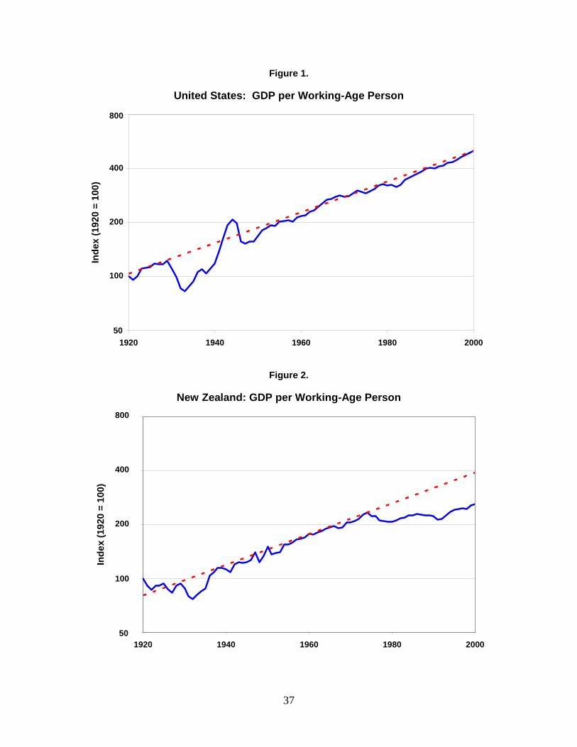
37
Figure 1.
United States: GDP per Working-Age Person
1920 1940 1960 1980 2000
Inde
x (1
920
= 10
0)
50
800
200
100
400
Figure 2.
New Zealand: GDP per Working-Age Person
1920 1940 1960 1980 2000
Inde
x (1
920
= 10
0)
200
50
100
400
800
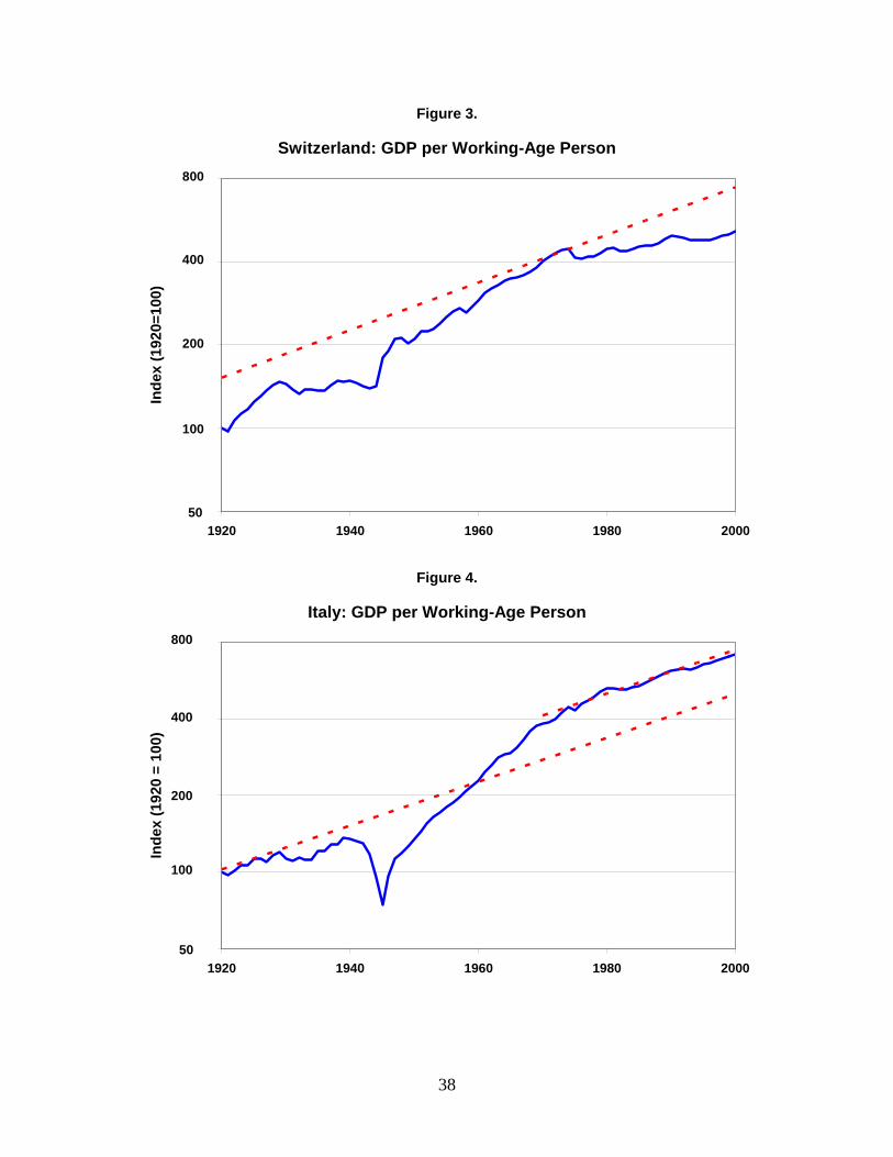
38
Figure 3.
Switzerland: GDP per Working-Age Person
1920 1940 1960 1980 2000
Inde
x (1
920=
100)
50
100
400
200
800
Figure 4.
Italy: GDP per Working-Age Person
1920 1940 1960 1980 2000
Inde
x (1
920
= 10
0)
50
800
400
200
100
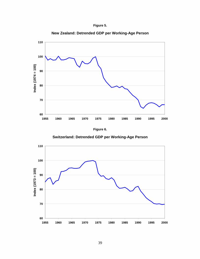
39
Figure 5.
New Zealand: Detrended GDP per Working-Age Person
60
70
80
90
100
110
1955 1960 1965 1970 1975 1980 1985 1990 1995 2000
Inde
x (1
974
= 10
0)
Figure 6.
Switzerland: Detrended GDP per Working-Age Person
60
70
80
90
100
110
1955 1960 1965 1970 1975 1980 1985 1990 1995 2000
Inde
x (1
973
= 10
0)
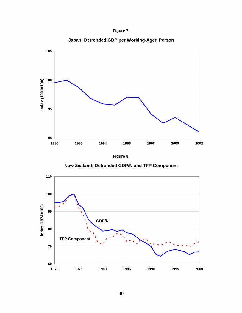
40
Figure 7.
Japan: Detrended GDP per Working-Aged Person
90
95
100
105
1990 1992 1994 1996 1998 2000 2002
Inde
x (1
991=
100)
Figure 8.
New Zealand: Detrended GDP/N and TFP Component
60
70
80
90
100
110
1970 1975 1980 1985 1990 1995 2000
inde
x (1
974=
100)
GDP/N
TFP Component
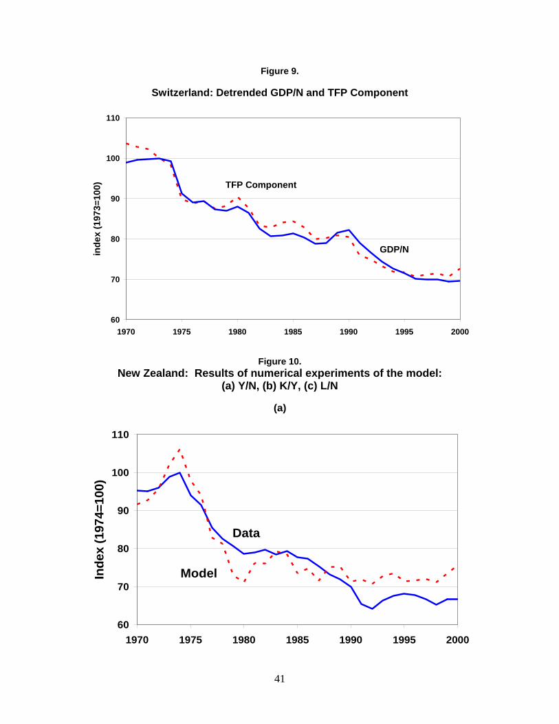
41
Figure 9.
Switzerland: Detrended GDP/N and TFP Component
60
70
80
90
100
110
1970 1975 1980 1985 1990 1995 2000
inde
x (1
973=
100)
GDP/N
TFP Component
Figure 10. New Zealand: Results of numerical experiments of the model:
(a) Y/N, (b) K/Y, (c) L/N
(a)
60
70
80
90
100
110
1970 1975 1980 1985 1990 1995 2000
Inde
x (1
974=
100)
Data
Model
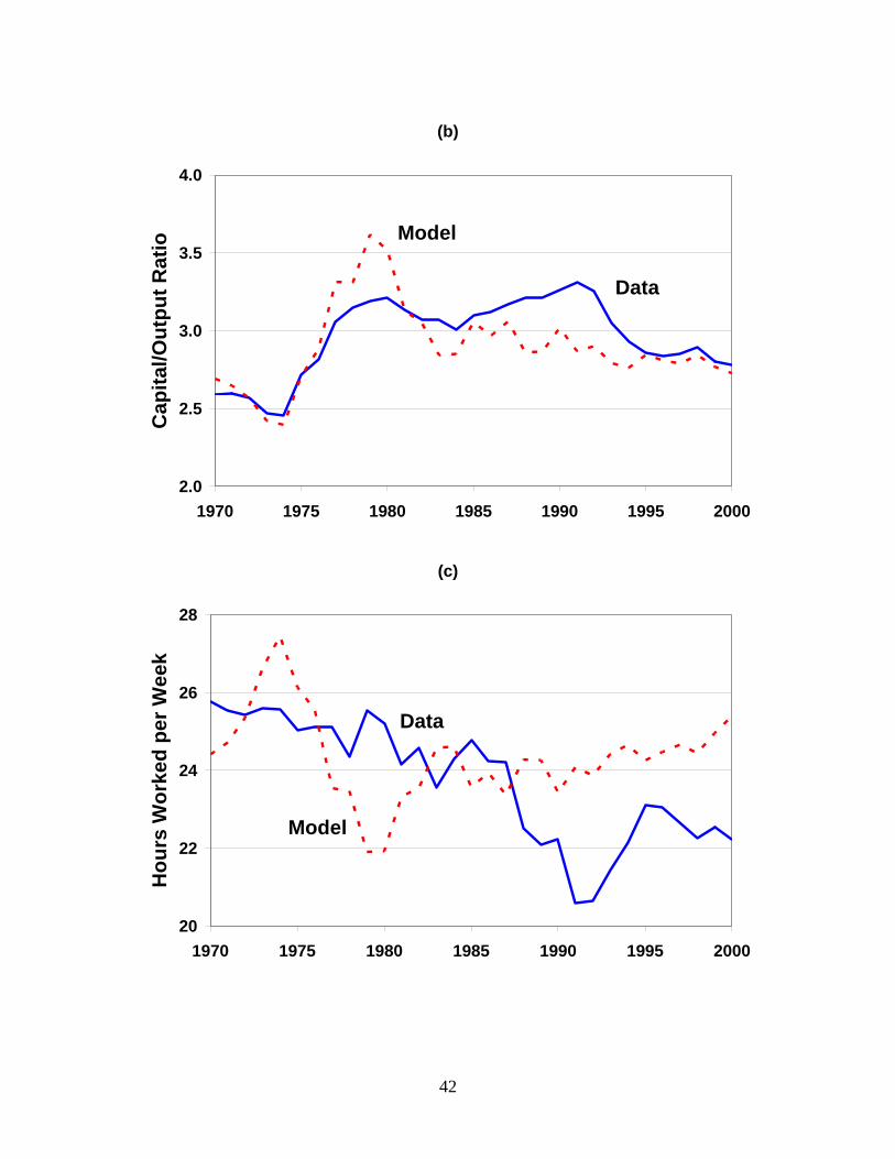
42
(b)
2.0
2.5
3.0
3.5
4.0
1970 1975 1980 1985 1990 1995 2000
Cap
ital/O
utpu
t Rat
io Model
Data
(c)
20
22
24
26
28
1970 1975 1980 1985 1990 1995 2000
Hou
rs W
orke
d pe
r Wee
k
Model
Data
43
Figure 11. Switzerland: Results of numerical experiments of the model:
(a) Y/N, (b) K/Y, (c) L/N
(a)
60
70
80
90
100
110
120
1970 1975 1980 1985 1990 1995 2000
Inde
x (1
973=
100)
Data
Model
(b)
2.5
3.0
3.5
4.0
1970 1975 1980 1985 1990 1995 2000
Cap
ital/O
utpu
t Rat
io
Model
Data
44
(c)
30
32
34
36
38
1970 1975 1980 1985 1990 1995 2000
Hou
rs W
orke
d pe
r Wee
k
Model
Data
Figure 12.
New Zealand: Price of Exports/Price of Imports
80
90
100
110
120
130
140
1955 1960 1965 1970 1975 1980 1985 1990 1995 2000
Inde
x (1
974=
100)
45
Figure 13.
United Kingdom's Share of New Zealand Trade
0
10
20
30
40
50
1965 1970 1975 1980 1985 1990 1995 2000
Shar
e of
Tot
al F
low
(%)
Exports
Imports
Figure 14.
United Kingdom's Share of Imported Capital Goods
0
10
20
30
40
50
60
1965 1970 1975 1980 1985 1990 1995 2000
Shar
e of
Tot
al F
low
(%)
Machinery and Transport Equipment (SITC 7)
46
Figure 15.
Switzerland: Price of Exports/Price of Imports
80
90
100
110
120
130
140
150
1970 1975 1980 1985 1990 1995 2000
Inde
x (1
973=
100)
Figure B1.
New Zealand: Different Measures of Population
60
70
80
90
100
110
1970 1975 1980 1985 1990 1995 2000
Inde
x (1
974=
100)
GDP/N
GDP/Capita
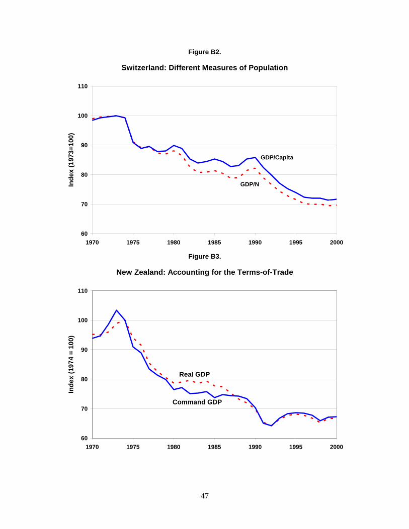
47
Figure B2.
Switzerland: Different Measures of Population
60
70
80
90
100
110
1970 1975 1980 1985 1990 1995 2000
Inde
x (1
973=
100)
GDP/Capita
GDP/N
Figure B3.
New Zealand: Accounting for the Terms-of-Trade
60
70
80
90
100
110
1970 1975 1980 1985 1990 1995 2000
Inde
x (1
974
= 10
0)
Real GDP
Command GDP
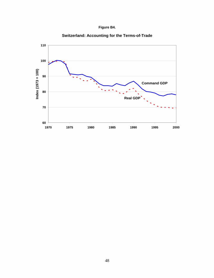
48
Figure B4.
Switzerland: Accounting for the Terms-of-Trade
60
70
80
90
100
110
1970 1975 1980 1985 1990 1995 2000
Inde
x (1
973
= 10
0)
Real GDP
Command GDP