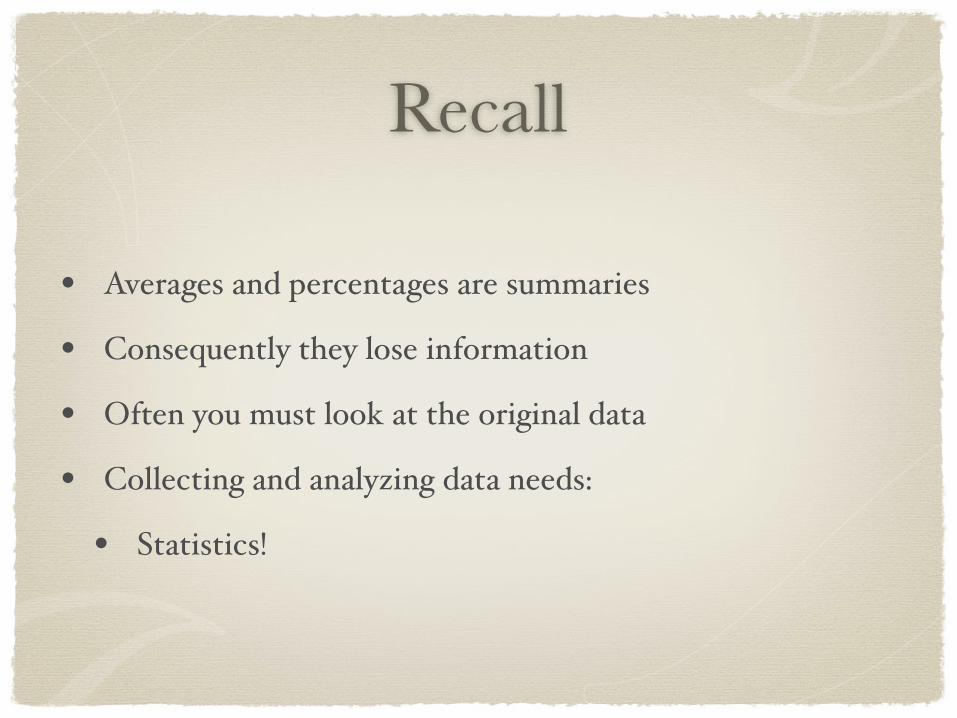
Recall

• Averages and percentages are summaries

• Consequently they lose information

• Often you must look at the original data

• Collecting and analyzing data needs:

• Statistics!

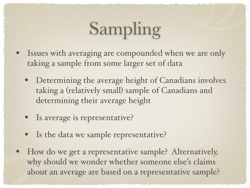
Sampling• Issues with averaging are compounded when we are only

taking a sample from some larger set of data

• Determining the average height of Canadians involves taking a (relatively small) sample of Canadians and determining their average height

• Is average is representative?

• Is the data we sample representative?

• How do we get a representative sample? Alternatively, why should we wonder whether someone else’s claims about an average are based on a representative sample?

Sampling

• Bad sampling can result from:

• having a biased selection technique

• getting unlucky

Sampling bias

• Any means of gathering data that tends towards an unrepresentative sample

• Using a university’s alumni donations address list for a survey on past student satisfaction

• An email survey measuring people’s level of comfort with technology

• A Sunday morning phone survey about church-going

• Voluntary responses in general

Sampling bias• Media:

• ‘unscientific’ polls

• screening calls (it’s a debate after all)

• sports reporting (x-game losing/winning streak)

• Red flags:

• Small samples (esp. of 1)

• Arbitrary cutoffs: “Last 17 years...”, “Since 1998...”

Sampling bias• Even without a biased sampling technique, we might just

get unlucky. Surveying height, we might happen to pick a set of people who are all taller than average, or shorter than average.

• How do we rule out being unlucky in this way?

• By taking the largest sample we can afford to take.

• By qualifying our confidence in our conclusions, according to the likelihood of getting unlucky with a sample of the size we chose.

Standard deviation

• Another kind of representative number:

• standard deviation (or variance)

• Definition:

• the average difference between the data points and the mean

• This reveals information about the distribution of the data points

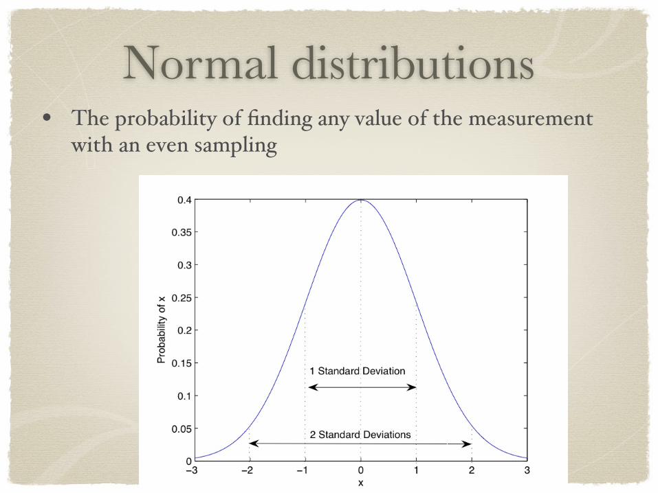
Normal distributions• The probability of finding any value of the measurement

with an even sampling

Normal distribution• What makes them normal (“Bell Curves”) is that they are

very common in many natural phenomenon

• Measuring height, weight, IQ, etc.

• Many yes/no decisions made randomly (50/50)

• The area under the curve is 1 (since any probability sums to 1).

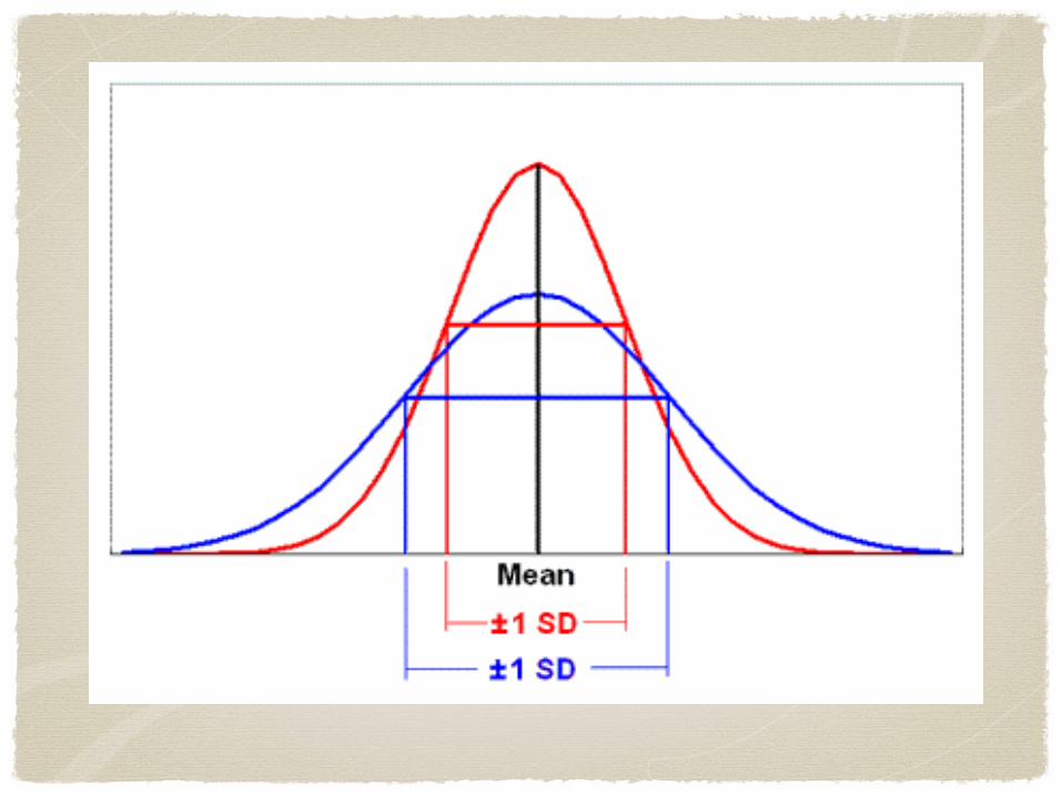
• Two distributions can be normal without being identical:

• a flatter curve has a larger standard deviation, while a taller curve has a smaller standard deviation

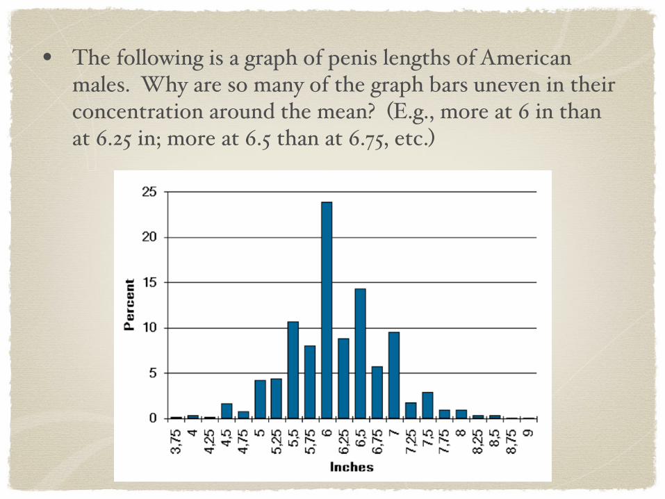
• The following is a graph of penis lengths of American males. Why are so many of the graph bars uneven in their concentration around the mean? (E.g., more at 6 in than at 6.25 in; more at 6.5 than at 6.75, etc.)

Confidence and error

• When we draw inferences from a set of data, we can only be confident in the conclusion to some degree

• Statistical significance:

• a measure of the confidence we are entitled to have in our probabilistic conclusion

• A function of how precise a conclusion we want

Significance

• Determination of correlation is relative to a nu! hypothesis

• null hypothesis: observed correlation is accidental

• Significance is measured by a p-value

• usually .01 or .05 (99% or 95% chance of data being non-random)

• Still need to figure out why it’s non-random (cause? common cause? other confound?)

Significance and error

• Confidence is cheap. We can always be 100% confident that the probability of some outcome is somewhere between 0 and 1 inclusive -- at the price of imprecision.

• The more precise we want our conclusion, the more data we need in order to have high confidence in it.

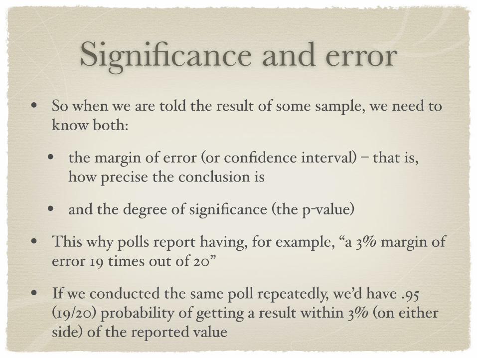
Significance and error• So when we are told the result of some sample, we need to

know both:

• the margin of error (or confidence interval) – that is, how precise the conclusion is

• and the degree of significance (the p-value)

• This why polls report having, for example, “a 3% margin of error 19 times out of 20”

• If we conducted the same poll repeatedly, we’d have .95 (19/20) probability of getting a result within 3% (on either side) of the reported value

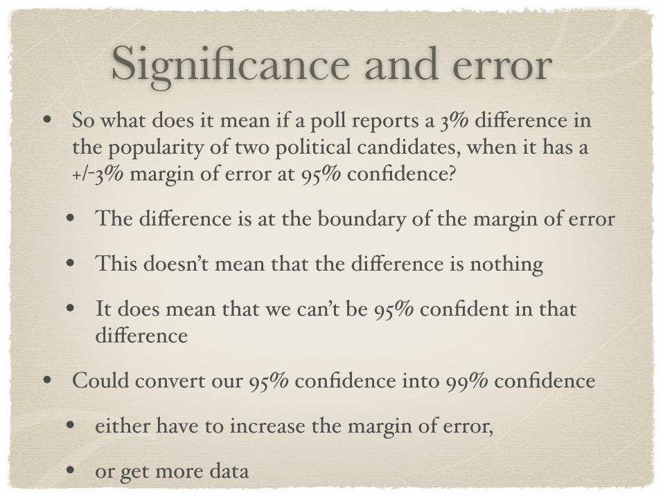
Significance and error• So what does it mean if a poll reports a 3% difference in

the popularity of two political candidates, when it has a +/-3% margin of error at 95% confidence?

• The difference is at the boundary of the margin of error

• This doesn’t mean that the difference is nothing

• It does mean that we can’t be 95% confident in that difference

• Could convert our 95% confidence into 99% confidence

• either have to increase the margin of error,

• or get more data

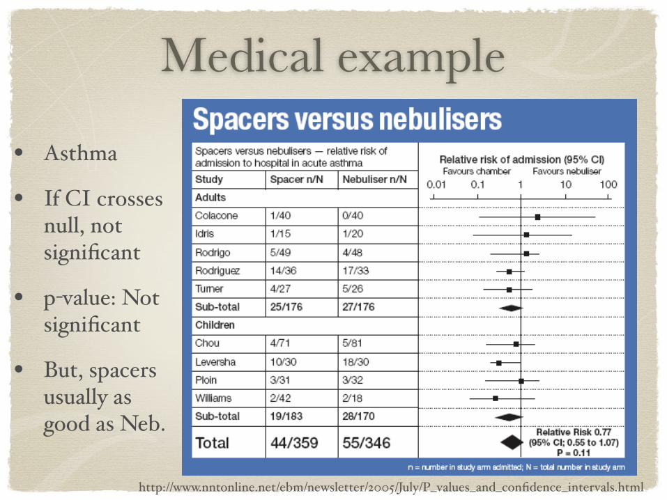
Medical example

http://www.nntonline.net/ebm/newsletter/2005/July/P_values_and_confidence_intervals.html

• Asthma

• If CI crosses null, not significant

• p-value: Not significant

• But, spacers usually as good as Neb.

Iraq mortality study• The Lancet 2004: The number of deaths additional to

what would have occurred without the invasion: 98,000.

• .95 confidence interval was 8,000-194,000.

• Widely reported as demonstrating a sloppy technique

• But at .90 CI the study shows a lower bound of approximately 40,000 additional deaths.

• Most confident of values at the centre of the CI

• The confidence tails off, but does not abruptly cease, as we consider outlying values of the CI

Summary

• A set of data permits you to be

• confident, to a degree

• precise, to a degree

• Understanding a statistical claim requires knowing both degrees

• Using fixed standards of significance (p-values) is the most common way of simplifying the interpretation of a statistical claim, but says nothing of effect size

Errors• There are two broad kinds of mistake we can make in

reasoning from a confidence level:

• Type I errors (false positives)

• Type II errors (false negatives)

• In a Type I error we have a random result that looks like a significant result

• In a Type II error we have a significant result that doesn’t get recognized as significant (or, more strongly, is categorized as random)

Errors

• In general we can only reduce the chances of one sort of error by either (1) improving our data or (2) increasing the odds of the other sort of error

• Ruling out legitimate voters versus allowing illegitimate voters

• Minimizing false accusations versus increasing unreported crime

• Reducing unnecessary treatments versus reducing undiagnosed illness

Terminology

• There may be an ambiguity in the term ‘significant’

• News stories often include phrases like, “Scientists reported that eating _____ had a significant effect in lowering the risks of ____”.

• But this could mean: A very tiny difference in probability was detected, but it was detected 19 times in 20.

Significance

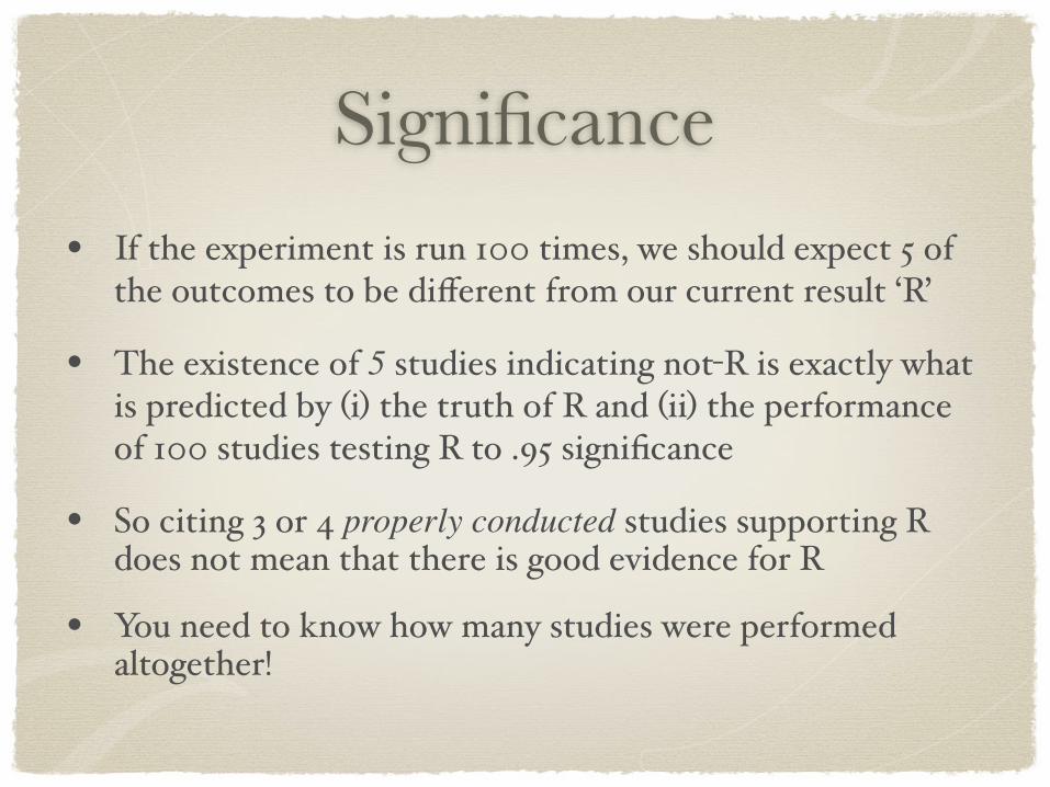
• If the experiment is run 100 times, we should expect 5 of the outcomes to be different from our current result ‘R’

• The existence of 5 studies indicating not-R is exactly what is predicted by (i) the truth of R and (ii) the performance of 100 studies testing R to .95 significance

• So citing 3 or 4 properly conducted studies supporting R does not mean that there is good evidence for R

• You need to know how many studies were performed altogether!

Consequences

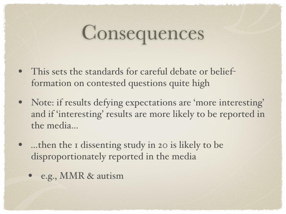
• This sets the standards for careful debate or belief-formation on contested questions quite high

• Note: if results defying expectations are ‘more interesting’ and if ‘interesting’ results are more likely to be reported in the media…

• …then the 1 dissenting study in 20 is likely to be disproportionately reported in the media

• e.g., MMR & autism

Probabilities

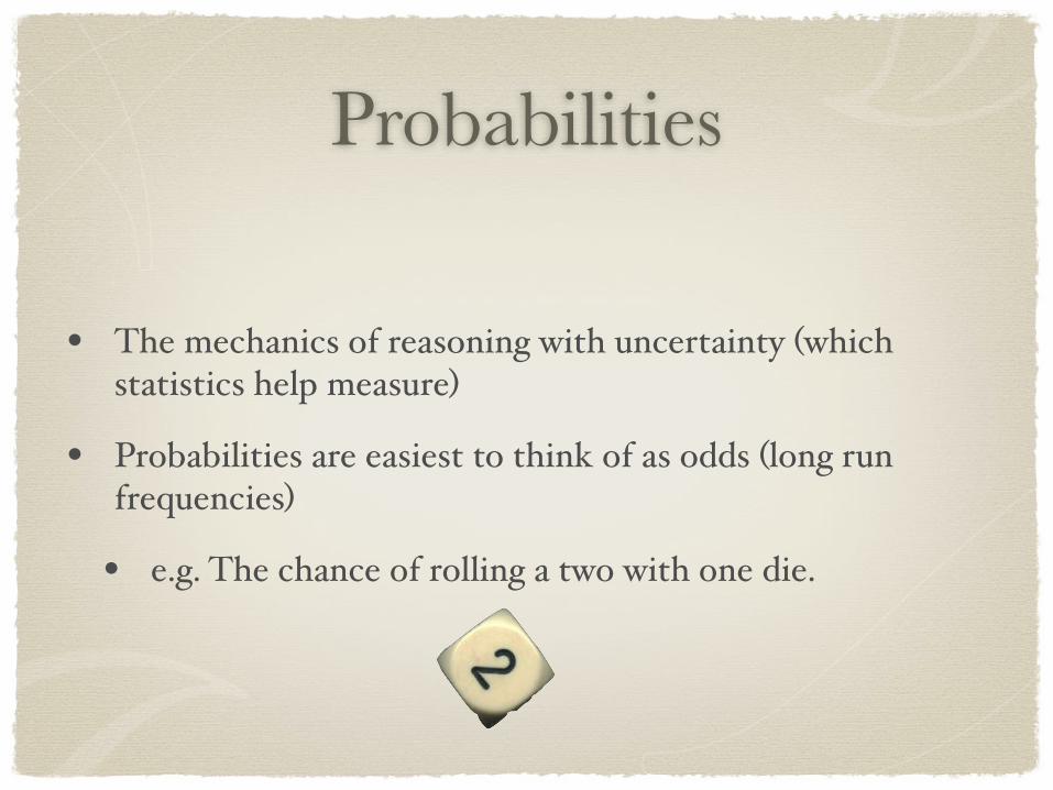
• The mechanics of reasoning with uncertainty (which statistics help measure)

• Probabilities are easiest to think of as odds (long run frequencies)

• e.g. The chance of rolling a two with one die.

Linda

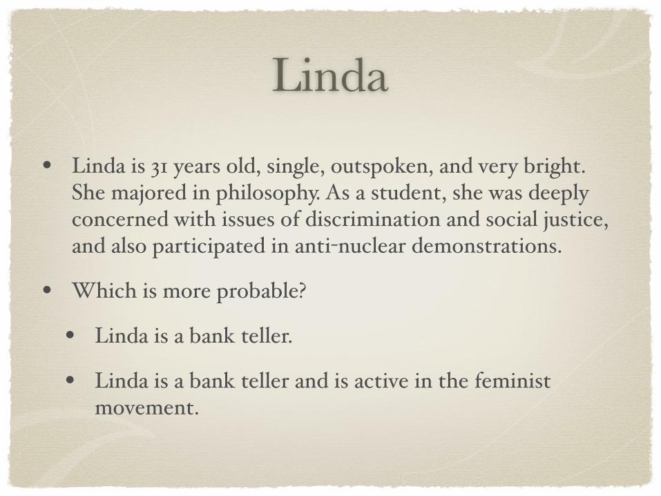
• Linda is 31 years old, single, outspoken, and very bright. She majored in philosophy. As a student, she was deeply concerned with issues of discrimination and social justice, and also participated in anti-nuclear demonstrations.

• Which is more probable?

• Linda is a bank teller.

• Linda is a bank teller and is active in the feminist movement.

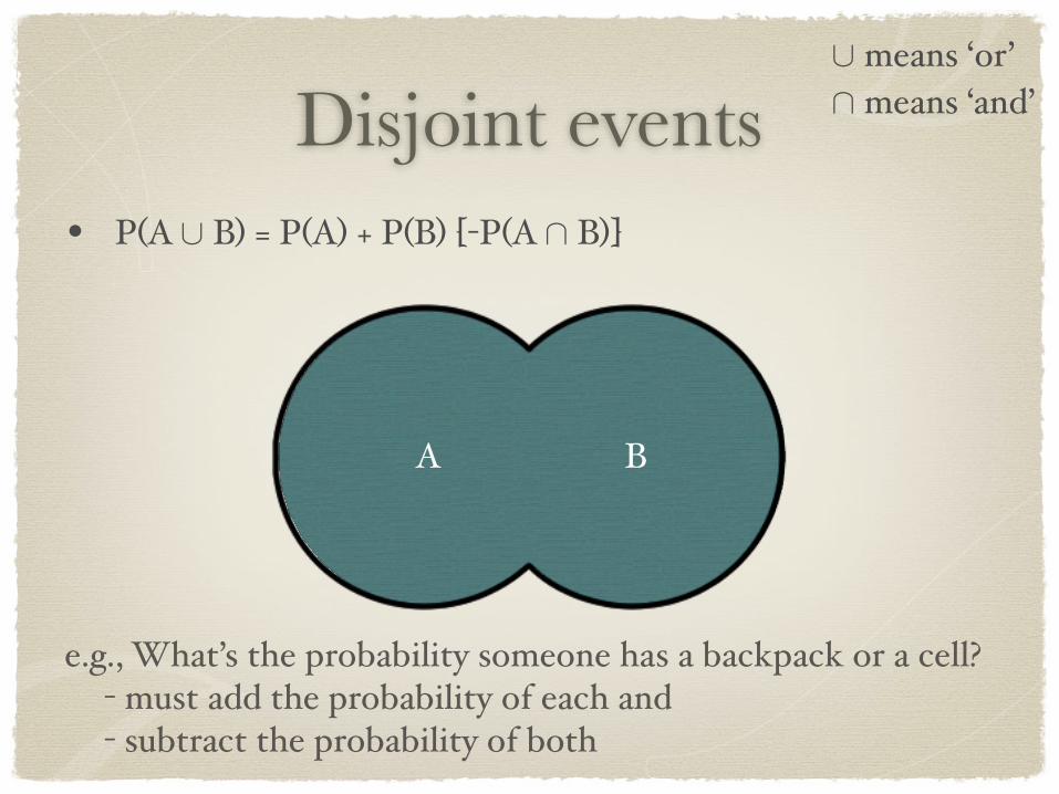
Disjoint events• P(A ∪ B) = P(A) + P(B) [-P(A ∩ B)]

A B

e.g., What’s the probability someone has a backpack or a cell?- must add the probability of each and - subtract the probability of both

∪ means ‘or’∩ means ‘and’

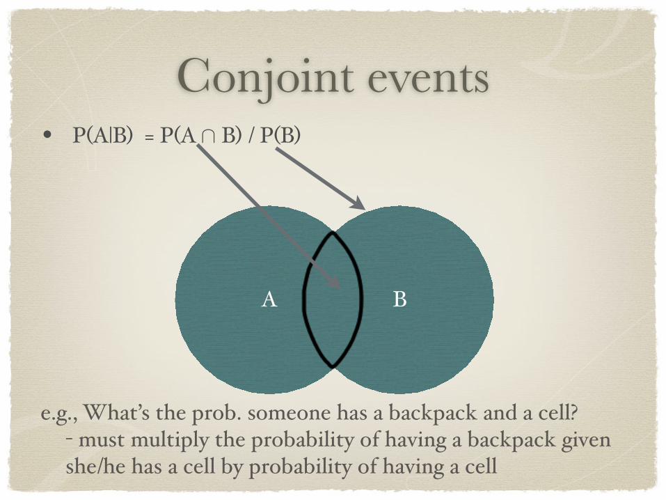
Conjoint events• P(A|B) = P(A ∩ B) / P(B)

A B

e.g., What’s the prob. someone has a backpack and a cell?- must multiply the probability of having a backpack given she/he has a cell by probability of having a cell

Conjoint events

• So, if events are independent (the conditional probability is zero) then P(A and B) = P(A)*P(B)

• This means that probabilities decrease quickly:

• If I’m 95% certain of each of W, X, Y, Z, then I’m only .95^4 = .81 or 81% certain of their conjunction

Conditional probabilities• Are what people often struggle with (e.g., no safe shelter

vs probability of being struck by lightning)

• Argument from Ignorance: need to know how hard we looked for the disconfirming evidence

• i.e., P(There’s no X | How hard we looked for evidence of X)

• Argument from Authority: need to know how good the authority is

• i.e., P(Conclusion | Goodness of authority)

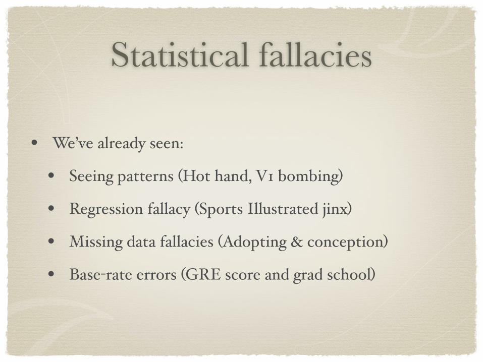
Statistical fallacies

• We’ve already seen:

• Seeing patterns (Hot hand, V1 bombing)

• Regression fallacy (Sports Illustrated jinx)

• Missing data fallacies (Adopting & conception)

• Base-rate errors (GRE score and grad school)

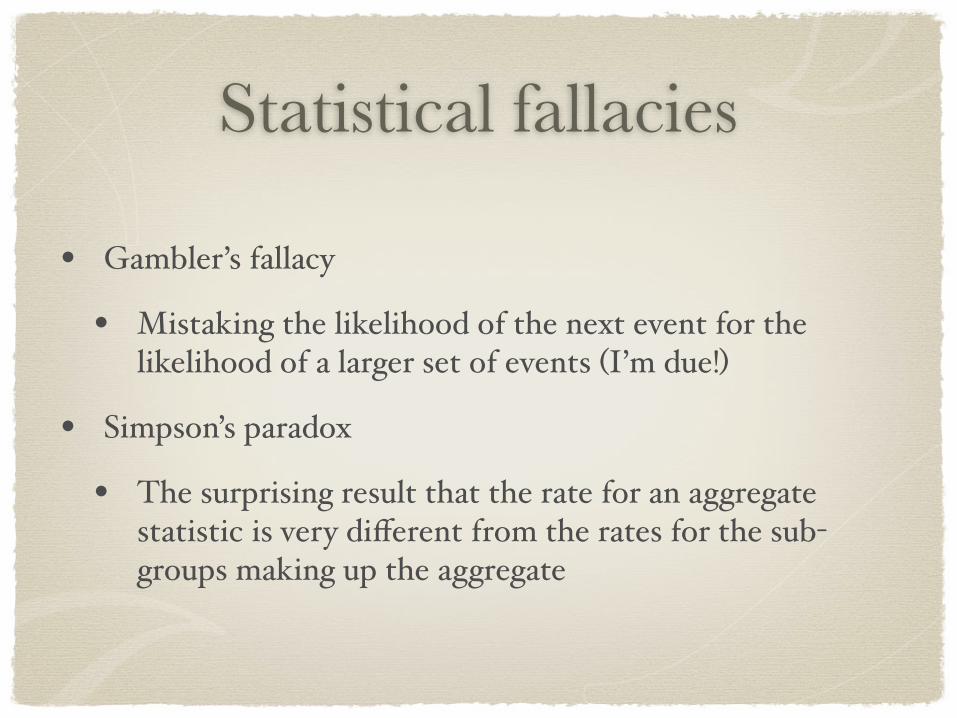
Statistical fallacies

• Gambler’s fallacy

• Mistaking the likelihood of the next event for the likelihood of a larger set of events (I’m due!)

• Simpson’s paradox

• The surprising result that the rate for an aggregate statistic is very different from the rates for the sub-groups making up the aggregate

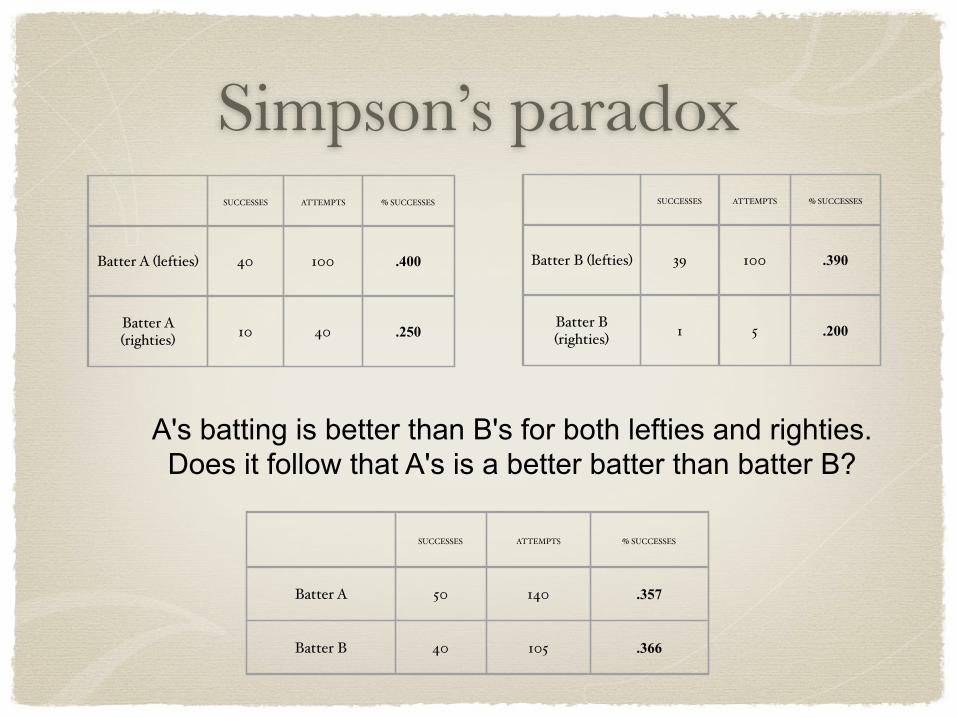
Simpson’s paradox  SUCCESSES ATTEMPTS % SUCCESSES

Batter A (lefties) 40 100 .400

Batter A (righties) 10 40 .250

 

  SUCCESSES ATTEMPTS % SUCCESSES

Batter B (lefties) 39 100 .390

Batter B (righties) 1 5 .200

A's batting is better than B's for both lefties and righties.Does it follow that A's is a better batter than batter B?

  SUCCESSES ATTEMPTS % SUCCESSES

Batter A 50 140 .357

Batter B 40 105 .366

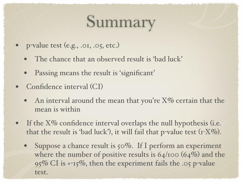
Summary• p-value test (e.g., .01, .05, etc.)

• The chance that an observed result is ‘bad luck’

• Passing means the result is ‘significant’

• Confidence interval (CI)

• An interval around the mean that you’re X% certain that the mean is within

• If the X% confidence interval overlaps the null hypothesis (i.e. that the result is ‘bad luck’), it will fail that p-value test (1-X%).

• Suppose a chance result is 50%. If I perform an experiment where the number of positive results is 64/100 (64%) and the 95% CI is +-15%, then the experiment fails the .05 p-value test.

Question

• Q: If you see a poll that reports a 2% difference between two candidates (19 times out of 20, with +/-3%) what can you be sure of? What can you not be sure of?