Embed Size (px)
Citation preview
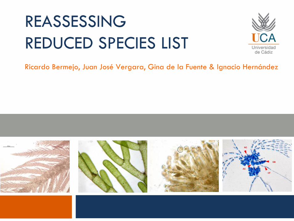
REASSESSING REDUCED SPECIES LISTRicardo Bermejo, Juan José Vergara, Gina de la Fuente & Ignacio Hernández
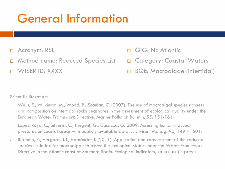
Acronym: RSL
Method name: Reduced Species List
WISER ID: XXXX
Scientific literature:
- Wells, E., Wilkinson, M., Wood, P., Scanlan, C. (2007). The use of macroalgal species richness and composition on intertidal rocky seashores in the assessment of ecological quality under the European Water Framework Directive. Marine Pollution Bulletin, 55: 151-161
- López-Royo, C., Silvestri, C., Pergent, G., Casazza, G. 2009. Assessing human-induced pressures on coastal areas with publicly available data. J. Environ. Manag. 90, 1494-1501.
- Bermejo, R., Vergara, J.J., Hernández I. (2011). Application and reassessment of the reduced species list index for macroalgae to assess the ecological status under the Water Framework Directive in the Atlantic coast of Southern Spain. Ecological Indicators, xx: xx-xx (in press)
General Information
GIG: NE Atlantic
Category: Coastal Waters
BQE: Macroalgae (intertidal)
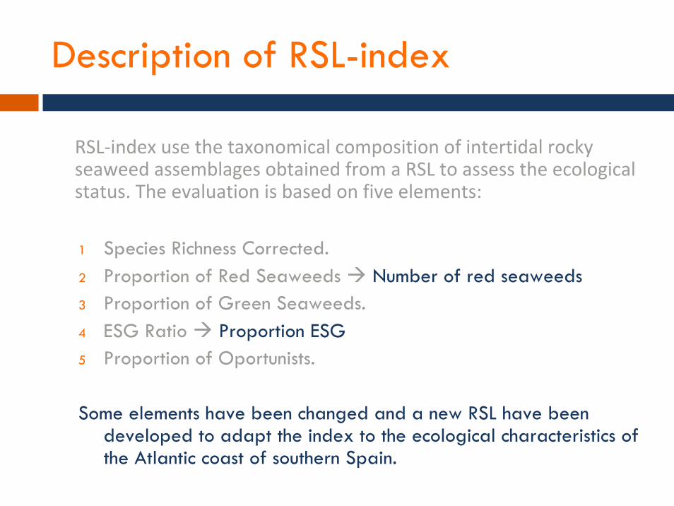
RSL‐index use the taxonomical composition of intertidal rocky seaweed assemblages obtained from a RSL to assess the ecologicalstatus. The evaluation is based on five elements:
1 Species Richness Corrected.2 Proportion of Red Seaweeds Number of red seaweeds 3 Proportion of Green Seaweeds. 4 ESG Ratio Proportion ESG 5 Proportion of Oportunists.
Some elements have been changed and a new RSL have been developed to adapt the index to the ecological characteristics of the Atlantic coast of southern Spain.
Description of RSL-index
3 ‐ Necessary informationMethodology
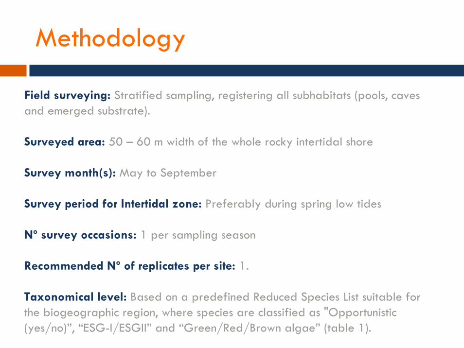
Field surveying: Stratified sampling, registering all subhabitats (pools, caves and emerged substrate).
Surveyed area: 50 – 60 m width of the whole rocky intertidal shore
Survey month(s): May to September
Survey period for Intertidal zone: Preferably during spring low tides
Nº survey occasions: 1 per sampling season
Recommended Nº of replicates per site: 1.
Taxonomical level: Based on a predefined Reduced Species List suitable for the biogeographic region, where species are classified as "Opportunistic (yes/no)”, “ESG-I/ESGII” and “Green/Red/Brown algae” (table 1).
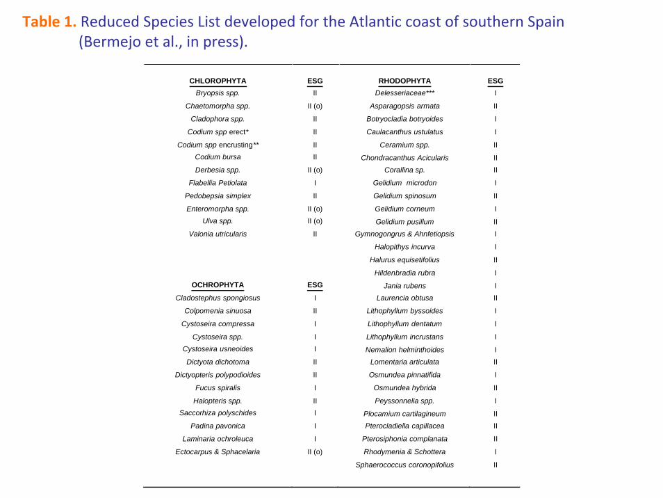
Table 1. Reduced Species List developed for the Atlantic coast of southern Spain (Bermejo et al., in press).
CHLOROPHYTA Bryopsis spp.
Chaetomorpha spp.
Cladophora spp.
Codium spp erect*
Codium spp encrusting** Codium bursa
Derbesia spp.
Flabellia Petiolata
Pedobepsia simplex
Enteromorpha spp. Ulva spp.
Valonia utricularis
OCHROPHYTA
Cladostephus spongiosus
Colpomenia sinuosa
Cystoseira compressa
Cystoseira spp. Cystoseira usneoides
Dictyota dichotoma
Dictyopteris polypodioides
Fucus spiralis
Halopteris spp. Saccorhiza polyschides
Padina pavonica
Laminaria ochroleuca
Ectocarpus & Sphacelaria
ESG II
II (o)
II
II
II II
II (o)
I
II
II (o) II (o)
II
ESG
I
II
I
I I
II
II
I
II I
I
I
II (o)
RHODOPHYTA Delesseriaceae***
Asparagopsis armata
Botryocladia botryoides
Caulacanthus ustulatus
Ceramium spp.
Chondracanthus Acicularis Corallina sp.
Gelidium microdon
Gelidium spinosum
Gelidium corneum
Gelidium pusillum Gymnogongrus & Ahnfetiopsis
Halopithys incurva
Halurus equisetifolius
Hildenbradia rubra
Jania rubens Laurencia obtusa
Lithophyllum byssoides
Lithophyllum dentatum
Lithophyllum incrustans
Nemalion helminthoides Lomentaria articulata
Osmundea pinnatifida
Osmundea hybrida
Peyssonnelia spp.
Plocamium cartilagineum Pterocladiella capillacea
Pterosiphonia complanata
Rhodymenia & Schottera
Sphaerococcus coronopifolius
ESG I
II
I
I
II
II II
I
II
I
II I
I
II
I
I II
I
I
I
I II
I
II
I
II II
II
I
II
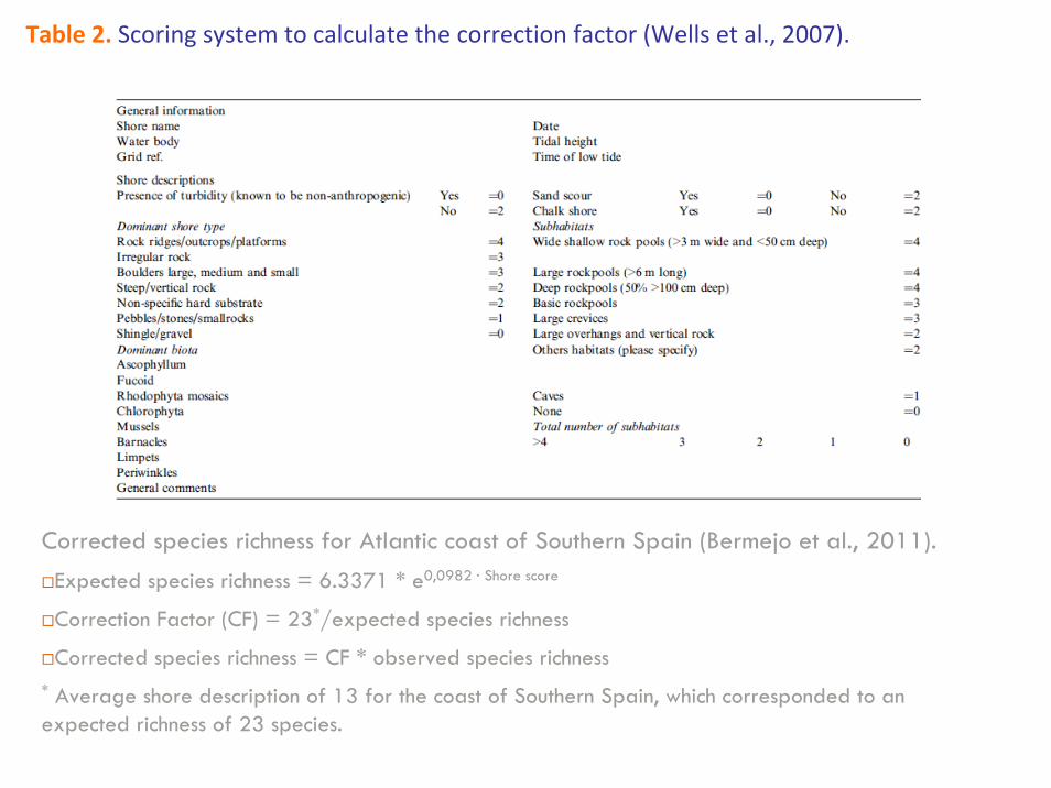
Corrected species richness for Atlantic coast of Southern Spain (Bermejo et al., 2011). Expected species richness = 6.3371 * e0,0982 · Shore score
Correction Factor (CF) = 23*/expected species richness
Corrected species richness = CF * observed species richness * Average shore description of 13 for the coast of Southern Spain, which corresponded to an expected richness of 23 species.
Table 2. Scoring system to calculate the correction factor (Wells et al., 2007).
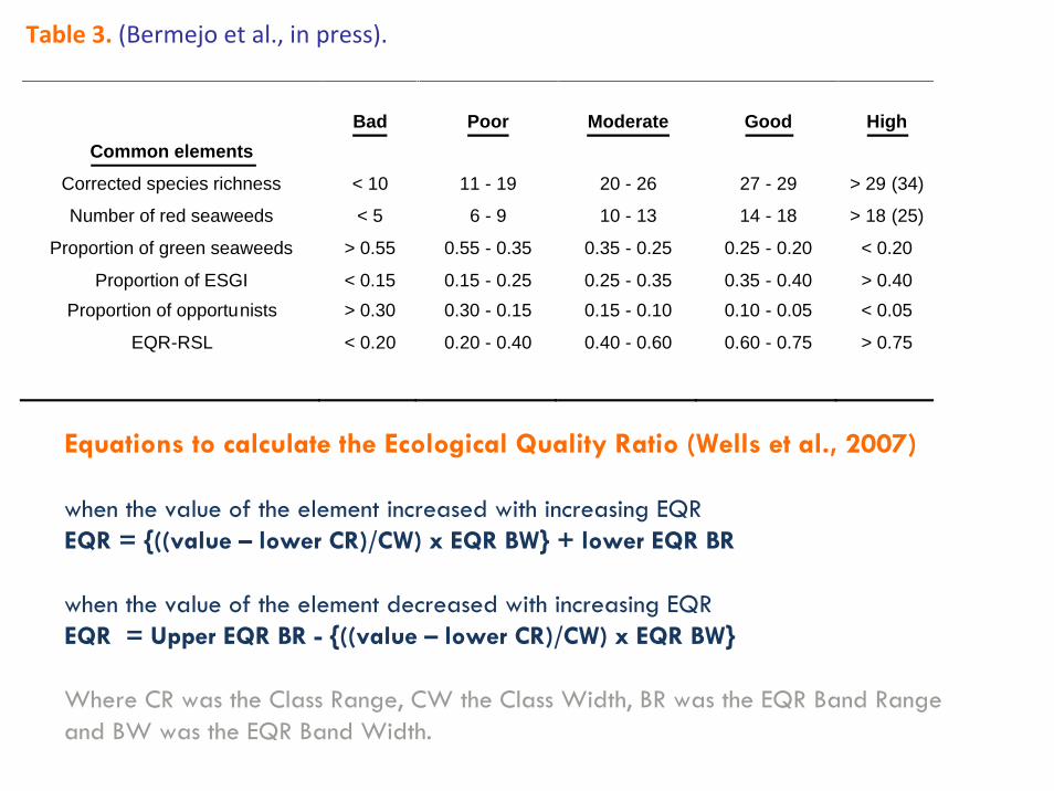
Equations to calculate the Ecological Quality Ratio (Wells et al., 2007)
when the value of the element increased with increasing EQREQR = {((value – lower CR)/CW) x EQR BW} + lower EQR BR
when the value of the element decreased with increasing EQREQR = Upper EQR BR - {((value – lower CR)/CW) x EQR BW}
Where CR was the Class Range, CW the Class Width, BR was the EQR Band Range and BW was the EQR Band Width.
Common elements
Table 3. (Bermejo et al., in press).
Corrected species richness
Number of red seaweeds
Proportion of green seaweeds
Proportion of ESGI Proportion of opportunists
EQR-RSL
Bad
< 10
< 5
> 0.55
< 0.15 > 0.30
< 0.20
Poor
11 - 19
6 - 9
0.55 - 0.35
0.15 - 0.25 0.30 - 0.15
0.20 - 0.40
Moderate
20 - 26
10 - 13
0.35 - 0.25
0.25 - 0.35 0.15 - 0.10
0.40 - 0.60
Good
27 - 29
14 - 18
0.25 - 0.20
0.35 - 0.40 0.10 - 0.05
0.60 - 0.75
High
> 29 (34)
> 18 (25)
< 0.20
> 0.40 < 0.05
> 0.75
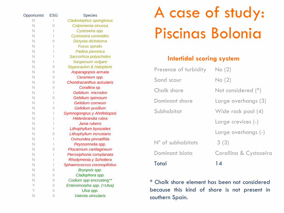
A case of study: Piscinas Bolonia
Presence of turbidity No (2)
Sand scour No (2)
Chalk shore Not considered (*)
Dominant shore Large overhangs (3)
Subhabitat Wide rock pool (4)
Large crevices (-)
Large overhangs (-)
Nº of subhabitats 3 (3)
Dominant biota Corallina & Cystoseira
Total 14
Intertidal scoring system
* Chalk shore element has been not considered because this kind of shore is not present in southern Spain.
Opportunist ESG Species N I Cladostephus spongiosus N II Colpomenia sinuosa N I Cystoseira spp. N I Cystoseira usneoides N II Dictyota dichotoma N I Fucus spiralis N I Padina pavonica N I Saccorhiza polyschides N I Sargassum vulgare N II Stypocaulon & Halopteris N II Asparagopsis armata N II Ceramium spp. N II Chondracanthus acicularis N II Corallina sp. N I Gelidium microdon N II Gelidium spinosum N I Gelidium corneum N II Gelidium pusillum N I Gymnogongrus y Ahnfetiopsis N I Hildenbrandia rubra N I Jania rubens N I Lithophyllum byssoides N II Lithophyllum incrustans N I Osmundea pinnatifida N I Peyssonnelia spp. N II Plocamium cartilagineum N I Pterosiphonia complanata N I Rhodymenia y Schottera N I Sphaerococcus coronopifolius N II Bryopsis spp. N II Cladophora spp. N II Codium spp encrusting** Y II Enteromorpha spp. (=Ulva) Y II Ulva spp. N II Valonia utricularis
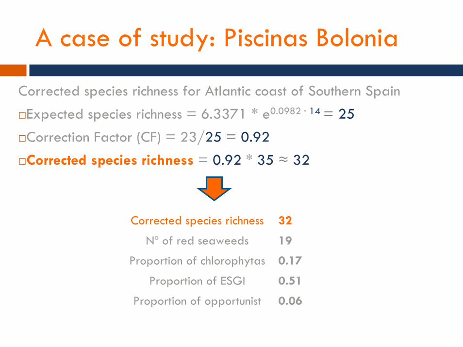
A case of study: Piscinas Bolonia
Corrected species richness for Atlantic coast of Southern Spain Expected species richness = 6.3371 * e0.0982 · 14 = 25Correction Factor (CF) = 23/25 = 0.92Corrected species richness = 0.92 * 35 ≈ 32
Corrected species richness 32
Nº of red seaweeds 19
Proportion of chlorophytas 0.17
Proportion of ESGI 0.51
Proportion of opportunist 0.06
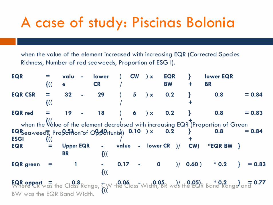
A case of study: Piscinas Bolonia
when the value of the element increased with increasing EQR (Corrected Species Richness, Number of red seaweeds, Proportion of ESG I).
EQR = {((
value
- lower CR
)/
CW ) x EQR BW
} +
lower EQR BR
EQR CSR = {((
32 - 29 )/
5 ) x 0.2 } +
0.8 = 0.84
EQR red = {((
19 - 18 )/
6 ) x 0.2 } +
0.8 = 0.83
EQR ESGI
= {((
0.51 - 0.40 )/
0.10 ) x 0.2 } +
0.8 = 0.84when the value of the element decreased with increasing EQR (Proportion of Green Seaweeds, Proportion of Opportunist)
Where CR was the Class Range, CW the Class Width, BR was the EQR Band Range and BW was the EQR Band Width.
EQR = Upper EQR BR
-{((
value - lower CR )/ CW) *EQR BW }
EQR green = 1 -{((
0.17 - 0 )/ 0.60 ) * 0.2 } = 0.83
EQR opport = 0.8 -{((
0.06 - 0.05 )/ 0.05) * 0.2 } = 0.77
A case of study: Piscinas Bolonia
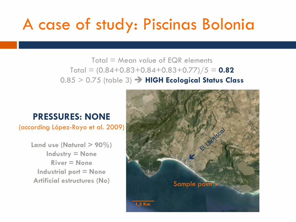
Total = Mean value of EQR elementsTotal = (0.84+0.83+0.84+0.83+0.77)/5 = 0.82
0.85 > 0.75 (table 3) HIGH Ecological Status Class
PRESSURES: NONE(according López-Royo et al. 2009)
Land use (Natural > 90%)Industry = None
River = NoneIndustrial port = None
Artificial estructures (No) Sample point x
El Len
tiscal
1,5 Km
A case of study: Puerto de Algeciras
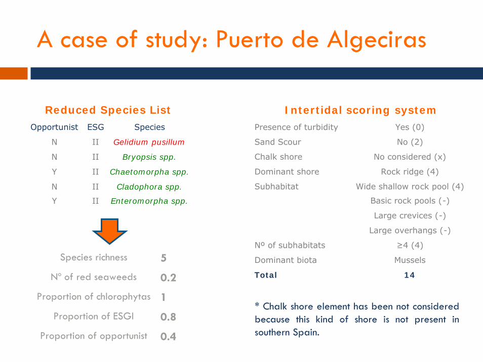
Reduced Species List Opportunist ESG Species
N II Gelidium pusillum
N II Bryopsis spp.
Y II Chaetomorpha spp.
N II Cladophora spp.
Y II Enteromorpha spp.
I ntert idal scoring system Presence of turbidity Yes (0)
Sand Scour No (2)
Chalk shore No considered (x)
Dominant shore Rock ridge (4)
Subhabitat Wide shallow rock pool (4)
Basic rock pools (-)
Large crevices (-)
Large overhangs (-)
Nº of subhabitats ≥4 (4)
Dominant biota Mussels
Total 1 4
* Chalk shore element has been not considered because this kind of shore is not present in southern Spain.
Species richness 5
Nº of red seaweeds 0.2
Proportion of chlorophytas 1
Proportion of ESGI 0.8
Proportion of opportunist 0.4
A case of study: Puerto de Algeciras
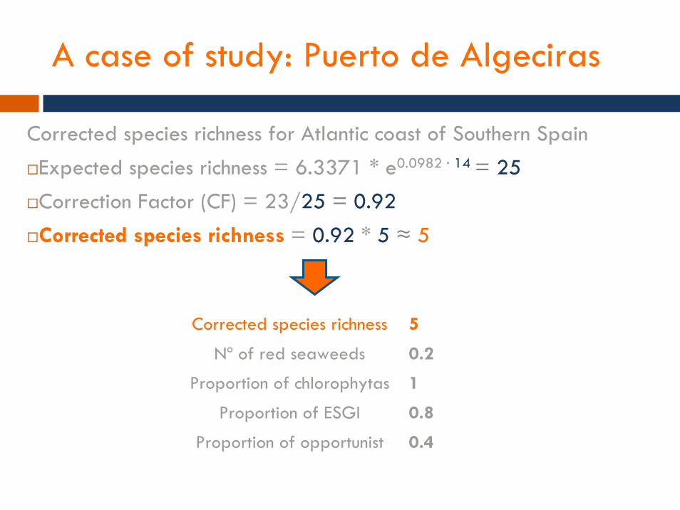
Corrected species richness for Atlantic coast of Southern Spain Expected species richness = 6.3371 * e0.0982 · 14 = 25Correction Factor (CF) = 23/25 = 0.92Corrected species richness = 0.92 * 5 ≈ 5
Corrected species richness 5
Nº of red seaweeds 0.2
Proportion of chlorophytas 1
Proportion of ESGI 0.8
Proportion of opportunist 0.4
A case of study: Puerto de Algeciras
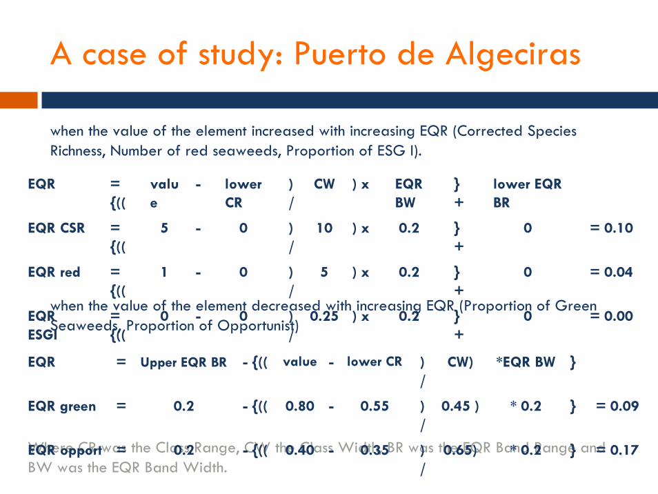
when the value of the element increased with increasing EQR (Corrected Species Richness, Number of red seaweeds, Proportion of ESG I).
EQR = {((
value
- lower CR
)/
CW ) x EQR BW
} +
lower EQR BR
EQR CSR = {((
5 - 0 )/
10 ) x 0.2 } +
0 = 0.10
EQR red = {((
1 - 0 )/
5 ) x 0.2 } +
0 = 0.04
EQR ESGI
= {((
0 - 0 )/
0.25 ) x 0.2 } +
0 = 0.00when the value of the element decreased with increasing EQR (Proportion of Green Seaweeds, Proportion of Opportunist)
Where CR was the Class Range, CW the Class Width, BR was the EQR Band Range and BW was the EQR Band Width.
EQR = Upper EQR BR - {(( value - lower CR )/
CW) *EQR BW }
EQR green = 0.2 - {(( 0.80 - 0.55 )/
0.45 ) * 0.2 } = 0.09
EQR opport = 0.2 - {(( 0.40 - 0.35 )/
0.65) * 0.2 } = 0.17
A case of study: Puerto de Algeciras
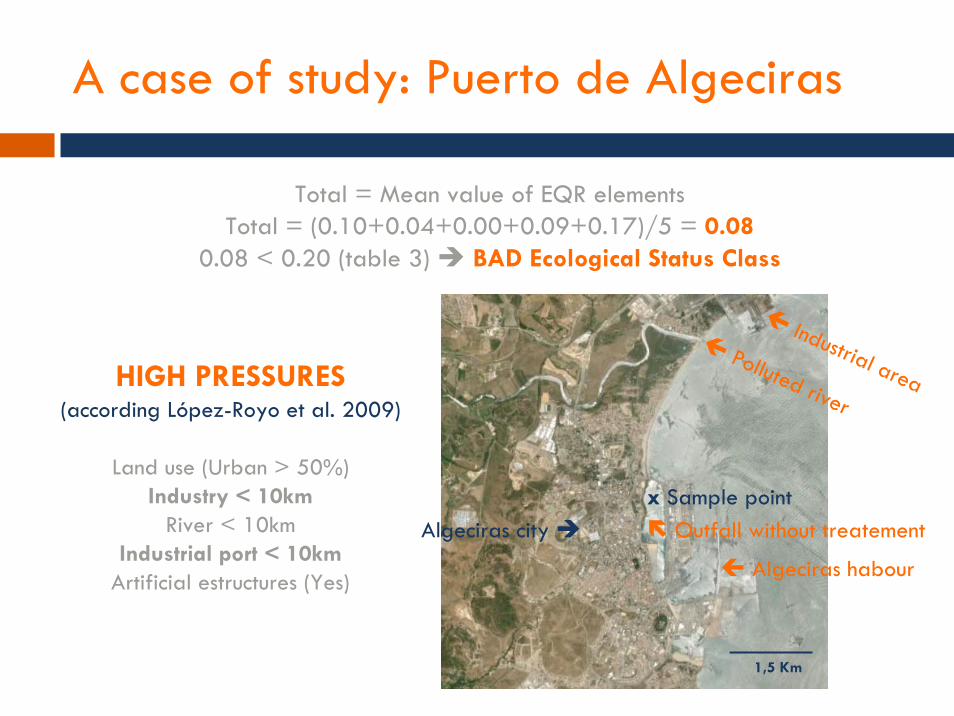
Total = Mean value of EQR elementsTotal = (0.10+0.04+0.00+0.09+0.17)/5 = 0.08
0.08 < 0.20 (table 3) BAD Ecological Status Class
Polluted river
Industrial area
Algeciras habour
Outfall without treatementAlgeciras cityx Sample point
1,5 Km
HIGH PRESSURES(according López-Royo et al. 2009)
Land use (Urban > 50%)Industry < 10km
River < 10kmIndustrial port < 10km
Artificial estructures (Yes)