Realtime Procedural Terrain Generation

Realtime Synthesis of Eroded Fractal Terrain for Use in Computer Games

Jacob Olsen, xenorg@imada.sdu.dkDepartment of Mathematics And Computer Science (IMADA)

University of Southern Denmark

October 31, 2004

Abstract

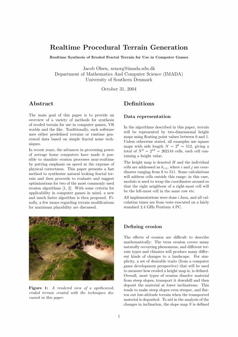
The main goal of this paper is to provide anoverview of a variety of methods for synthesisof eroded terrain for use in computer games, VRworlds and the like. Traditionally, such softwareuses either predefined terrains or runtime gen-erated data based on simple fractal noise tech-niques.In recent years, the advances in processing powerof average home computers have made it pos-sible to simulate erosion processes near-realtimeby putting emphasis on speed at the expense ofphysical correctness. This paper presents a fastmethod to synthesize natural looking fractal ter-rain and then proceeds to evaluate and suggestoptimizations for two of the most commonly usederosion algorithms [1, 2]. With some criteria forapplicability in computer games in mind, a newand much faster algorithm is then proposed. Fi-nally, a few issues regarding terrain modificationsfor maximum playability are discussed.

Figure 1: A rendered view of a synthesized,eroded terrain created with the techniques dis-cussed in this paper.

Definitions

Data representation

In the algorithms described in this paper, terrainwill be represented by two-dimensional heightmaps using floating point values between 0 and 1.Unless otherwise stated, all examples use squaremaps with side length N = 29 = 512, giving atotal of N2 = 218 = 262144 cells, each cell con-taining a height value.

The height map is denoted H and the individualcells are addressed as hi,j , where i and j are coor-dinates ranging from 0 to 511. Some calculationswill address cells outside this range; in this case,modulo is used to wrap the coordinates around sothat the right neighbour of a right-most cell willbe the left-most cell in the same row etc.

All implementations were done i Java, and all cal-culation times are from tests executed on a fairlystandard 2.4 GHz Pentium 4 PC.

Defining erosion

The effects of erosion are difficult to describemathematically: The term erosion covers manynaturally occurring phenomena, and different ter-rain types and climates will produce many differ-ent kinds of changes to a landscape. For sim-plicity, a set of desirable traits (from a computergame development perspective) that will be usedto measure how eroded a height map is, is defined.Overall, most types of erosion dissolve materialfrom steep slopes, transport it downhill and thendeposit the material at lower inclinations. Thistends to make steep slopes even steeper, and flat-ten out low-altitude terrain when the transportedmaterial is deposited. To aid in the analysis of thechanges in inclination, the slope map S is defined

1

such that

si,j = max(|hi,j − hi−1,j |,|hi,j − hi+1,j |,|hi,j − hi,j−1|,|hi,j − hi,j+1|)

in other words, the greatest of the height differ-ences between the cell and its four neighbours ina Von Neumann neighbourhood.This paper focuses on the synthesis of eroded ter-rain for use in computer games; therefore, theideal for eroded terrain must suit this applica-tion. Physical correctness and visual appearanceare secondary, what matters is applicability. Inmost computer games and VR environments us-ing large-scale outdoor terrain, persons or vehiclesmove around on the terrain, and various struc-tures are placed on the terrain. Movement andstructure placing is often restricted to low incli-nations, which means that a low average valueof a height map’s corresponding slope map is de-sirable. This rule alone would make a perfectlyflat height map ideal, which is why a second ruleis added saying the greater the standard devia-tion of the slope map, the better. The ideal foreroded terrain is therefore a height map whosecorresponding slope map has a low mean value(reflecting the overall flattening of the terrain dueto material deposition) and a high standard devi-ation (material is dissolved from steep areas mak-ing them even steeper, and deposition flattens theflat areas further). The slope map mean value, s,and standard deviation, σs, are defined on theslope map S as follows:

s =1

N2

N−1∑i=0

N−1∑j=0

si,j

σs =

√√√√ 1N2

N−1∑i=0

N−1∑j=0

(si,j − s)2

Using these, an overall ”erosion score”, ε, is de-fined as

ε =σs

s

(on the assumption that s 6= 0)

Generation of base terrain

A technique often used for fast terrain genera-tion is simulating 1/f noise (also known as ”pinknoise”) which is characterized by the spectral en-ergy density being proportional to the reciprocal

of the frequency, i.e.

P (f) =1fa

where P (f) is the power function of the frequencyand a is close to 1. This kind of noise approx-imates real-world uneroded mountainous terrainwell and has been used widely in computer graph-ics for the past decades. Two methods for gener-ating 1/f -like noise, spectral synthesis and mid-point displacement, are discussed below.In generating a terrain base for the erosion al-gorithms to work on, it is worth noting that thecloser the terrain base is to the desired result,the less work is required by the (often calculationheavy) erosion algorithm itself. To help create aterrain base with better characteristics of erodedterrain, the use of Voronoi diagrams and pertur-bation filtering are introduced below.

Spectral synthesis

Spectral synthesis simulates 1/f noise by addingseveral octaves (layers) together, each octave con-sisting of noise with all its spectral energy concen-trated on a single frequency. For each octave, thenoise frequency is doubled and the amplitude Ais calculated by

A = pi

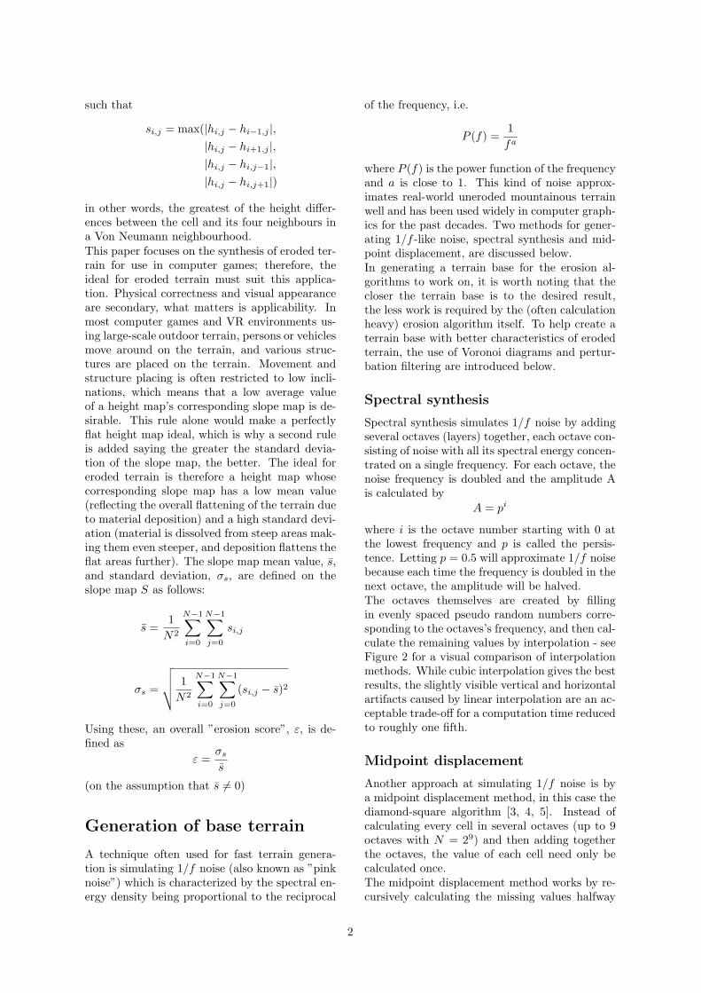
where i is the octave number starting with 0 atthe lowest frequency and p is called the persis-tence. Letting p = 0.5 will approximate 1/f noisebecause each time the frequency is doubled in thenext octave, the amplitude will be halved.The octaves themselves are created by fillingin evenly spaced pseudo random numbers corre-sponding to the octaves’s frequency, and then cal-culate the remaining values by interpolation - seeFigure 2 for a visual comparison of interpolationmethods. While cubic interpolation gives the bestresults, the slightly visible vertical and horizontalartifacts caused by linear interpolation are an ac-ceptable trade-off for a computation time reducedto roughly one fifth.

Midpoint displacement

Another approach at simulating 1/f noise is bya midpoint displacement method, in this case thediamond-square algorithm [3, 4, 5]. Instead ofcalculating every cell in several octaves (up to 9octaves with N = 29) and then adding togetherthe octaves, the value of each cell need only becalculated once.The midpoint displacement method works by re-cursively calculating the missing values halfway

2

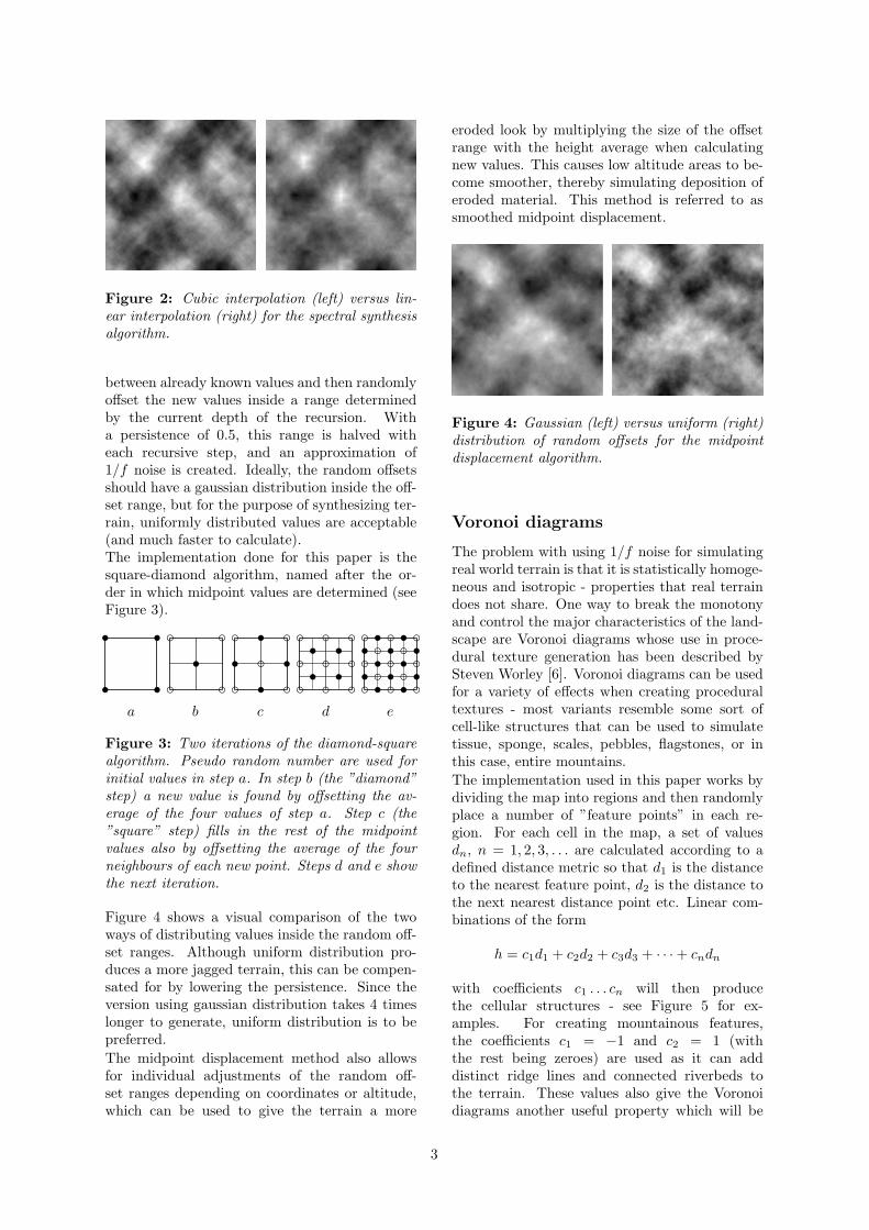
Figure 2: Cubic interpolation (left) versus lin-ear interpolation (right) for the spectral synthesisalgorithm.

between already known values and then randomlyoffset the new values inside a range determinedby the current depth of the recursion. Witha persistence of 0.5, this range is halved witheach recursive step, and an approximation of1/f noise is created. Ideally, the random offsetsshould have a gaussian distribution inside the off-set range, but for the purpose of synthesizing ter-rain, uniformly distributed values are acceptable(and much faster to calculate).The implementation done for this paper is thesquare-diamond algorithm, named after the or-der in which midpoint values are determined (seeFigure 3).

ss

ss

cc

ccs c

ccccs s

s s cc

cccc c

c cs ss scc

cccc c

c cc cc cs ss s ss ss s ss s

a b c d e

Figure 3: Two iterations of the diamond-squarealgorithm. Pseudo random number are used forinitial values in step a. In step b (the ”diamond”step) a new value is found by offsetting the av-erage of the four values of step a. Step c (the”square” step) fills in the rest of the midpointvalues also by offsetting the average of the fourneighbours of each new point. Steps d and e showthe next iteration.

Figure 4 shows a visual comparison of the twoways of distributing values inside the random off-set ranges. Although uniform distribution pro-duces a more jagged terrain, this can be compen-sated for by lowering the persistence. Since theversion using gaussian distribution takes 4 timeslonger to generate, uniform distribution is to bepreferred.The midpoint displacement method also allowsfor individual adjustments of the random off-set ranges depending on coordinates or altitude,which can be used to give the terrain a more

eroded look by multiplying the size of the offsetrange with the height average when calculatingnew values. This causes low altitude areas to be-come smoother, thereby simulating deposition oferoded material. This method is referred to assmoothed midpoint displacement.

Figure 4: Gaussian (left) versus uniform (right)distribution of random offsets for the midpointdisplacement algorithm.

Voronoi diagrams

The problem with using 1/f noise for simulatingreal world terrain is that it is statistically homoge-neous and isotropic - properties that real terraindoes not share. One way to break the monotonyand control the major characteristics of the land-scape are Voronoi diagrams whose use in proce-dural texture generation has been described bySteven Worley [6]. Voronoi diagrams can be usedfor a variety of effects when creating proceduraltextures - most variants resemble some sort ofcell-like structures that can be used to simulatetissue, sponge, scales, pebbles, flagstones, or inthis case, entire mountains.The implementation used in this paper works bydividing the map into regions and then randomlyplace a number of ”feature points” in each re-gion. For each cell in the map, a set of valuesdn, n = 1, 2, 3, . . . are calculated according to adefined distance metric so that d1 is the distanceto the nearest feature point, d2 is the distance tothe next nearest distance point etc. Linear com-binations of the form

h = c1d1 + c2d2 + c3d3 + · · ·+ cndn

with coefficients c1 . . . cn will then producethe cellular structures - see Figure 5 for ex-amples. For creating mountainous features,the coefficients c1 = −1 and c2 = 1 (withthe rest being zeroes) are used as it can adddistinct ridge lines and connected riverbeds tothe terrain. These values also give the Voronoidiagrams another useful property which will be

3

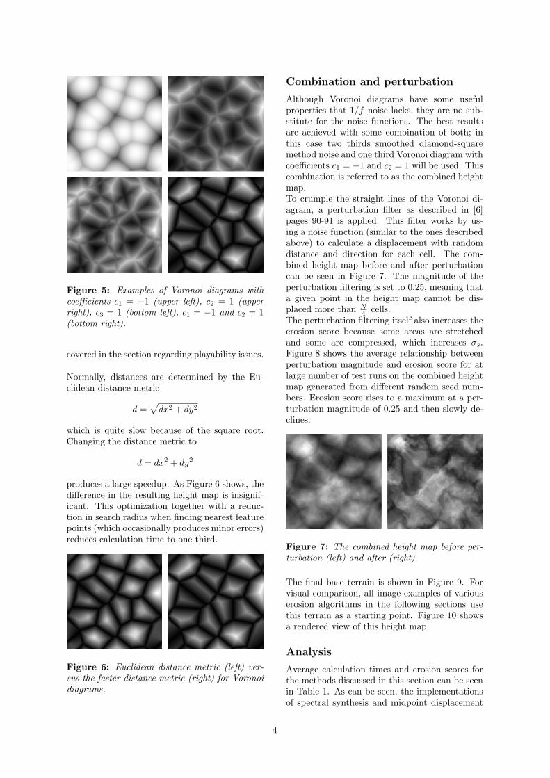
Figure 5: Examples of Voronoi diagrams withcoefficients c1 = −1 (upper left), c2 = 1 (upperright), c3 = 1 (bottom left), c1 = −1 and c2 = 1(bottom right).

covered in the section regarding playability issues.

Normally, distances are determined by the Eu-clidean distance metric

d =√

dx2 + dy2

which is quite slow because of the square root.Changing the distance metric to

d = dx2 + dy2

produces a large speedup. As Figure 6 shows, thedifference in the resulting height map is insignif-icant. This optimization together with a reduc-tion in search radius when finding nearest featurepoints (which occasionally produces minor errors)reduces calculation time to one third.

Figure 6: Euclidean distance metric (left) ver-sus the faster distance metric (right) for Voronoidiagrams.

Combination and perturbation

Although Voronoi diagrams have some usefulproperties that 1/f noise lacks, they are no sub-stitute for the noise functions. The best resultsare achieved with some combination of both; inthis case two thirds smoothed diamond-squaremethod noise and one third Voronoi diagram withcoefficients c1 = −1 and c2 = 1 will be used. Thiscombination is referred to as the combined heightmap.To crumple the straight lines of the Voronoi di-agram, a perturbation filter as described in [6]pages 90-91 is applied. This filter works by us-ing a noise function (similar to the ones describedabove) to calculate a displacement with randomdistance and direction for each cell. The com-bined height map before and after perturbationcan be seen in Figure 7. The magnitude of theperturbation filtering is set to 0.25, meaning thata given point in the height map cannot be dis-placed more than N

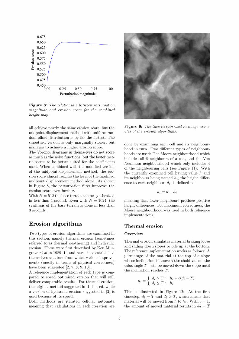
4 cells.The perturbation filtering itself also increases theerosion score because some areas are stretchedand some are compressed, which increases σs.Figure 8 shows the average relationship betweenperturbation magnitude and erosion score for atlarge number of test runs on the combined heightmap generated from different random seed num-bers. Erosion score rises to a maximum at a per-turbation magnitude of 0.25 and then slowly de-clines.

Figure 7: The combined height map before per-turbation (left) and after (right).

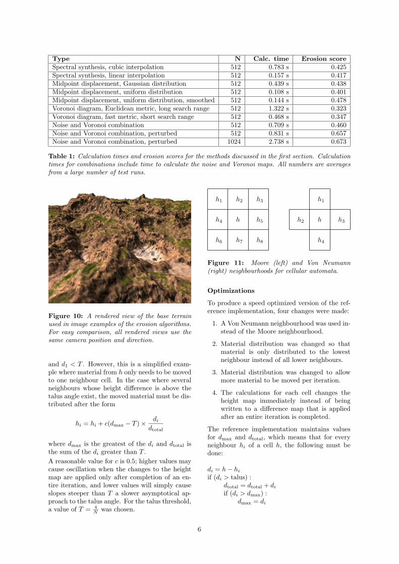
The final base terrain is shown in Figure 9. Forvisual comparison, all image examples of variouserosion algorithms in the following sections usethis terrain as a starting point. Figure 10 showsa rendered view of this height map.

Analysis

Average calculation times and erosion scores forthe methods discussed in this section can be seenin Table 1. As can be seen, the implementationsof spectral synthesis and midpoint displacement

4

0.00 0.25 0.50 0.75 1.000.450

0.475

0.500

0.525

0.550

0.575

0.600

0.625

0.650

0.675

Perturbation magnitude

Ero

sion

sco

re

Figure 8: The relationship between perturbationmagnitude and erosion score for the combinedheight map.

all achieve nearly the same erosion score, but themidpoint displacement method with uniform ran-dom offset distribution is by far the fastest. Thesmoothed version is only marginally slower, butmanages to achieve a higher erosion score.The Voronoi diagrams in themselves do not scoreas much as the noise functions, but the faster met-ric seems to be better suited for the coefficientsused. When combined with the modified versionof the midpoint displacement method, the ero-sion score almost reaches the level of the modifiedmidpoint displacement method alone. As shownin Figure 8, the perturbation filter improves theerosion score even further.With N = 512 the base terrain can be synthesizedin less than 1 second. Even with N = 1024, thesynthesis of the base terrain is done in less than3 seconds.

Erosion algorithms

Two types of erosion algorithms are examined inthis section, namely thermal erosion (sometimesreferred to as thermal weathering) and hydraulicerosion. These were first described by Ken Mus-grave et al in 1989 [1], and have since establishedthemselves as a base from which various improve-ments (mostly in terms of physical correctness)have been suggested [2, 7, 8, 9, 10].A reference implementation of each type is com-pared to speed optimized version that will stilldeliver comparable results. For thermal erosion,the original method suggested in [1] is used, whilea version of hydraulic erosion suggested in [2] isused because of its speed.Both methods are iterated cellular automatameaning that calculations in each iteration are

Figure 9: The base terrain used in image exam-ples of the erosion algorithms.

done by examining each cell and its neighbour-hood in turn. Two different types of neighbour-hoods are used: The Moore neighbourhood whichincludes all 8 neighbours of a cell, and the VonNeumann neighbourhood which only includes 4of the neighbouring cells (see Figure 11). Withthe currently examined cell having value h andits neighbours being named hi, the height differ-ence to each neighbour, di, is defined as

di = h− hi

meaning that lower neighbours produce positiveheight differences. For maximum correctness, theMoore neighbourhood was used in both referenceimplementations.

Thermal erosion

Overview

Thermal erosion simulates material braking looseand sliding down slopes to pile up at the bottom.The reference implementation works as follows: Apercentage of the material at the top of a slopewhose inclination is above a threshold value - thetalus angle T - will be moved down the slope untilthe inclination reaches T :

hi ={

di > T : hi + c(di − T )di ≤ T : hi

This is illustrated in Figure 12: At the firsttimestep, d1 = T and d2 > T , which means thatmaterial will be moved from h to h2. With c = 1,the amount of moved material results in d2 = T

5

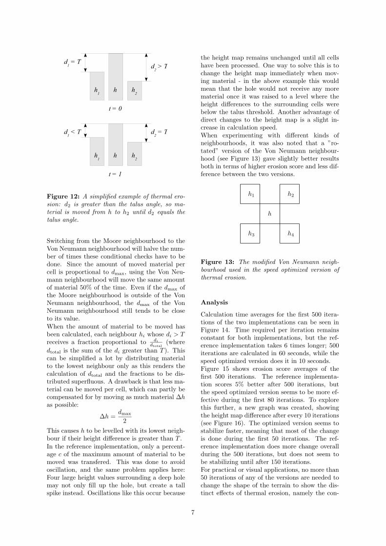
Type N Calc. time Erosion scoreSpectral synthesis, cubic interpolation 512 0.783 s 0.425Spectral synthesis, linear interpolation 512 0.157 s 0.417Midpoint displacement, Gaussian distribution 512 0.439 s 0.438Midpoint displacement, uniform distribution 512 0.108 s 0.401Midpoint displacement, uniform distribution, smoothed 512 0.144 s 0.478Voronoi diagram, Euclidean metric, long search range 512 1.322 s 0.323Voronoi diagram, fast metric, short search range 512 0.468 s 0.347Noise and Voronoi combination 512 0.709 s 0.460Noise and Voronoi combination, perturbed 512 0.831 s 0.657Noise and Voronoi combination, perturbed 1024 2.738 s 0.673

Table 1: Calculation times and erosion scores for the methods discussed in the first section. Calculationtimes for combinations include time to calculate the noise and Voronoi maps. All numbers are averagesfrom a large number of test runs.

Figure 10: A rendered view of the base terrainused in image examples of the erosion algorithms.For easy comparison, all rendered views use thesame camera position and direction.

and d1 < T . However, this is a simplified exam-ple where material from h only needs to be movedto one neighbour cell. In the case where severalneighbours whose height difference is above thetalus angle exist, the moved material must be dis-tributed after the form

hi = hi + c(dmax − T )× di

dtotal

where dmax is the greatest of the di and dtotal isthe sum of the di greater than T .A reasonable value for c is 0.5; higher values maycause oscillation when the changes to the heightmap are applied only after completion of an en-tire iteration, and lower values will simply causeslopes steeper than T a slower asymptotical ap-proach to the talus angle. For the talus threshold,a value of T = 4

N was chosen.

h1 h2 h3

h4 h h5

h6 h7 h8

h1

h2 h h3

h4

Figure 11: Moore (left) and Von Neumann(right) neighbourhoods for cellular automata.

Optimizations

To produce a speed optimized version of the ref-erence implementation, four changes were made:

1. A Von Neumann neighbourhood was used in-stead of the Moore neighbourhood.

2. Material distribution was changed so thatmaterial is only distributed to the lowestneighbour instead of all lower neighbours.

3. Material distribution was changed to allowmore material to be moved per iteration.

4. The calculations for each cell changes theheight map immediately instead of beingwritten to a difference map that is appliedafter an entire iteration is completed.

The reference implementation maintains valuesfor dmax and dtotal, which means that for everyneighbour hi of a cell h, the following must bedone:

di = h− hi

if (di > talus) :dtotal = dtotal + di

if (di > dmax) :dmax = di

6

h1

h h2

h1

h h2

d1 = T

d2 > T

t = 0

t = 1

d2 = Td

1 < T

Figure 12: A simplified example of thermal ero-sion: d2 is greater than the talus angle, so ma-terial is moved from h to h2 until d2 equals thetalus angle.

Switching from the Moore neighbourhood to theVon Neumann neighbourhood will halve the num-ber of times these conditional checks have to bedone. Since the amount of moved material percell is proportional to dmax, using the Von Neu-mann neighbourhood will move the same amountof material 50% of the time. Even if the dmax ofthe Moore neighbourhood is outside of the VonNeumann neighbourhood, the dmax of the VonNeumann neighbourhood still tends to be closeto its value.When the amount of material to be moved hasbeen calculated, each neighbour hi whose di > Treceives a fraction proportional to di

dtotal(where

dtotal is the sum of the di greater than T ). Thiscan be simplified a lot by distributing materialto the lowest neighbour only as this renders thecalculation of dtotal and the fractions to be dis-tributed superfluous. A drawback is that less ma-terial can be moved per cell, which can partly becompensated for by moving as much material ∆has possible:

∆h =dmax

2

This causes h to be levelled with its lowest neigh-bour if their height difference is greater than T .In the reference implementation, only a percent-age c of the maximum amount of material to bemoved was transfered. This was done to avoidoscillation, and the same problem applies here:Four large height values surrounding a deep holemay not only fill up the hole, but create a tallspike instead. Oscillations like this occur because

the height map remains unchanged until all cellshave been processed. One way to solve this is tochange the height map immediately when mov-ing material - in the above example this wouldmean that the hole would not receive any morematerial once it was raised to a level where theheight differences to the surrounding cells werebelow the talus threshold. Another advantage ofdirect changes to the height map is a slight in-crease in calculation speed.When experimenting with different kinds ofneighbourhoods, it was also noted that a ”ro-tated” version of the Von Neumann neighbour-hood (see Figure 13) gave slightly better resultsboth in terms of higher erosion score and less dif-ference between the two versions.

h1 h2

h

h3 h4

Figure 13: The modified Von Neumann neigh-bourhood used in the speed optimized version ofthermal erosion.

Analysis

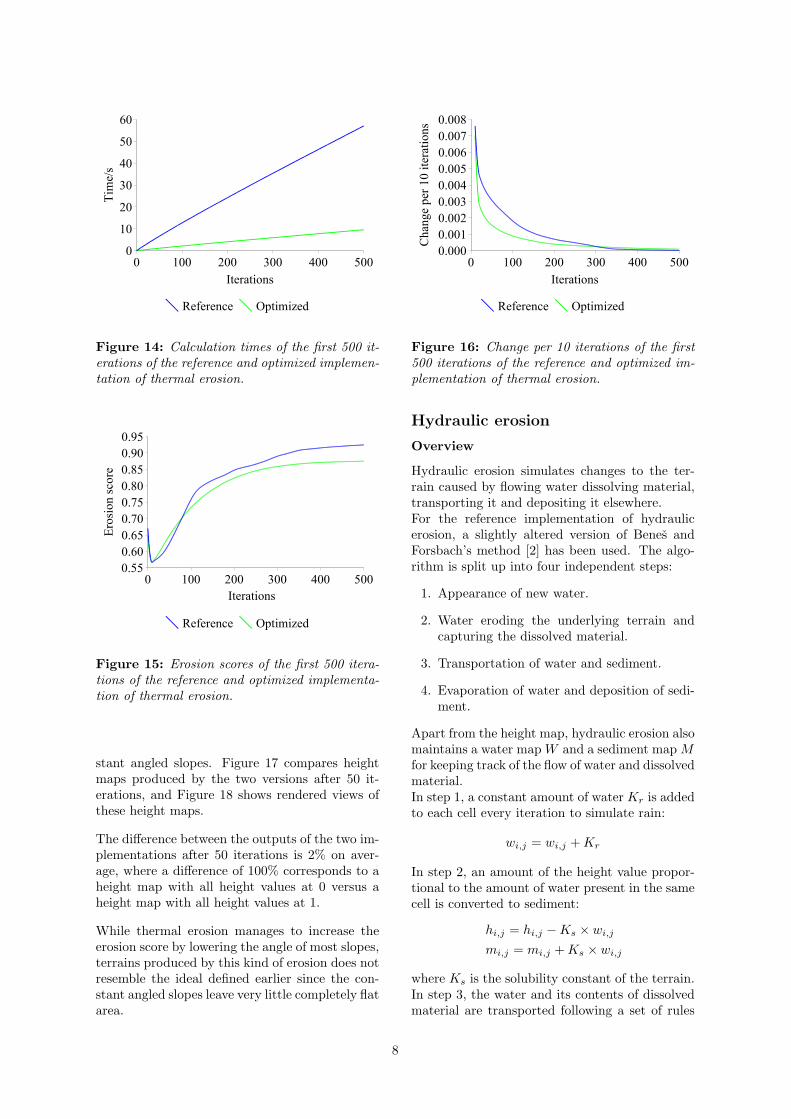
Calculation time averages for the first 500 itera-tions of the two implementations can be seen inFigure 14. Time required per iteration remainsconstant for both implementations, but the ref-erence implementation takes 6 times longer; 500iterations are calculated in 60 seconds, while thespeed optimized version does it in 10 seconds.Figure 15 shows erosion score averages of thefirst 500 iterations. The reference implementa-tion scores 5% better after 500 iterations, butthe speed optimized version seems to be more ef-fective during the first 80 iterations. To explorethis further, a new graph was created, showingthe height map difference after every 10 iterations(see Figure 16). The optimized version seems tostabilize faster, meaning that most of the changeis done during the first 50 iterations. The ref-erence implementation does more change overallduring the 500 iterations, but does not seem tobe stabilizing until after 150 iterations.For practical or visual applications, no more than50 iterations of any of the versions are needed tochange the shape of the terrain to show the dis-tinct effects of thermal erosion, namely the con-

7

0 100 200 300 400 5000

10

20

30

40

50

60

Reference Optimized

Iterations

Time/s

Figure 14: Calculation times of the first 500 it-erations of the reference and optimized implemen-tation of thermal erosion.

0 100 200 300 400 5000.550.600.650.700.750.800.850.900.95

Reference Optimized

Iterations

Ero

sion

sco

re

Figure 15: Erosion scores of the first 500 itera-tions of the reference and optimized implementa-tion of thermal erosion.

stant angled slopes. Figure 17 compares heightmaps produced by the two versions after 50 it-erations, and Figure 18 shows rendered views ofthese height maps.

The difference between the outputs of the two im-plementations after 50 iterations is 2% on aver-age, where a difference of 100% corresponds to aheight map with all height values at 0 versus aheight map with all height values at 1.

While thermal erosion manages to increase theerosion score by lowering the angle of most slopes,terrains produced by this kind of erosion does notresemble the ideal defined earlier since the con-stant angled slopes leave very little completely flatarea.

0 100 200 300 400 5000.0000.0010.0020.0030.0040.0050.0060.0070.008

Reference Optimized

Iterations

Cha

nge

per

10 it

erat

ions

Figure 16: Change per 10 iterations of the first500 iterations of the reference and optimized im-plementation of thermal erosion.

Hydraulic erosion

Overview

Hydraulic erosion simulates changes to the ter-rain caused by flowing water dissolving material,transporting it and depositing it elsewhere.For the reference implementation of hydraulicerosion, a slightly altered version of Benes andForsbach’s method [2] has been used. The algo-rithm is split up into four independent steps:

1. Appearance of new water.

2. Water eroding the underlying terrain andcapturing the dissolved material.

3. Transportation of water and sediment.

4. Evaporation of water and deposition of sedi-ment.

Apart from the height map, hydraulic erosion alsomaintains a water map W and a sediment map Mfor keeping track of the flow of water and dissolvedmaterial.In step 1, a constant amount of water Kr is addedto each cell every iteration to simulate rain:

wi,j = wi,j + Kr

In step 2, an amount of the height value propor-tional to the amount of water present in the samecell is converted to sediment:

hi,j = hi,j −Ks × wi,j

mi,j = mi,j + Ks × wi,j

where Ks is the solubility constant of the terrain.In step 3, the water and its contents of dissolvedmaterial are transported following a set of rules

8

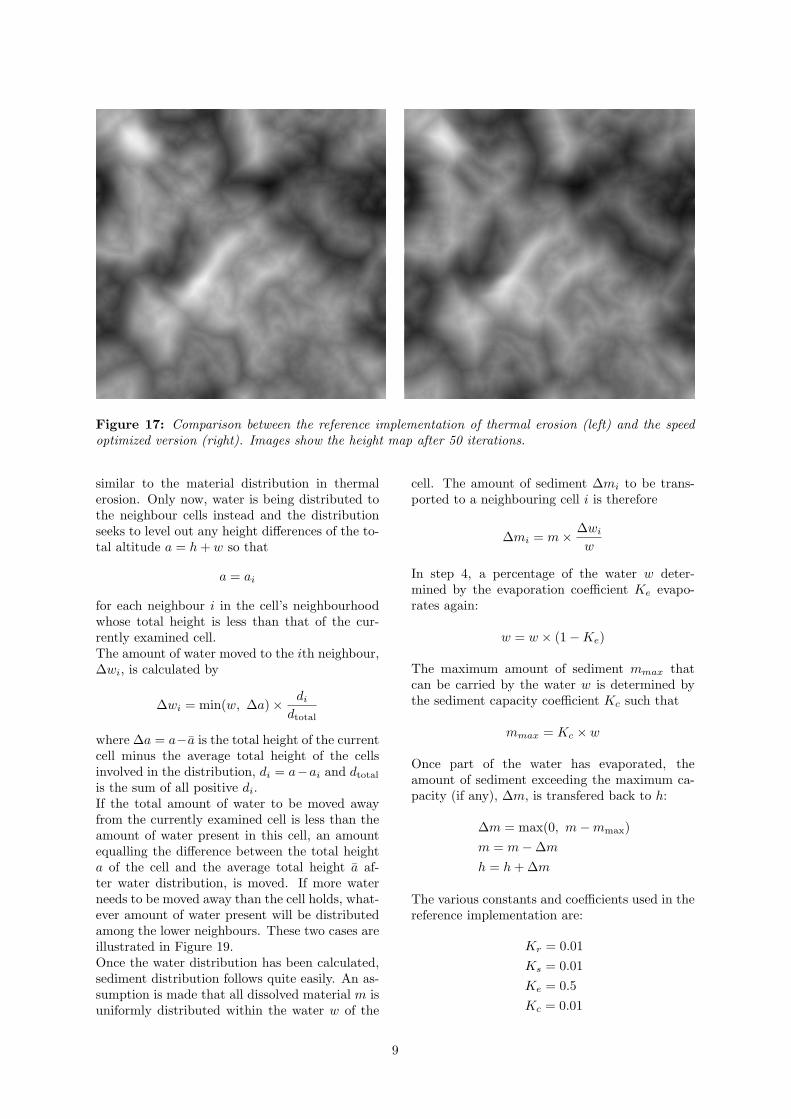
Figure 17: Comparison between the reference implementation of thermal erosion (left) and the speedoptimized version (right). Images show the height map after 50 iterations.

similar to the material distribution in thermalerosion. Only now, water is being distributed tothe neighbour cells instead and the distributionseeks to level out any height differences of the to-tal altitude a = h + w so that

a = ai

for each neighbour i in the cell’s neighbourhoodwhose total height is less than that of the cur-rently examined cell.The amount of water moved to the ith neighbour,∆wi, is calculated by

∆wi = min(w, ∆a)× di

dtotal

where ∆a = a−a is the total height of the currentcell minus the average total height of the cellsinvolved in the distribution, di = a−ai and dtotal

is the sum of all positive di.If the total amount of water to be moved awayfrom the currently examined cell is less than theamount of water present in this cell, an amountequalling the difference between the total heighta of the cell and the average total height a af-ter water distribution, is moved. If more waterneeds to be moved away than the cell holds, what-ever amount of water present will be distributedamong the lower neighbours. These two cases areillustrated in Figure 19.Once the water distribution has been calculated,sediment distribution follows quite easily. An as-sumption is made that all dissolved material m isuniformly distributed within the water w of the

cell. The amount of sediment ∆mi to be trans-ported to a neighbouring cell i is therefore

∆mi = m× ∆wi

w

In step 4, a percentage of the water w deter-mined by the evaporation coefficient Ke evapo-rates again:

w = w × (1−Ke)

The maximum amount of sediment mmax thatcan be carried by the water w is determined bythe sediment capacity coefficient Kc such that

mmax = Kc × w

Once part of the water has evaporated, theamount of sediment exceeding the maximum ca-pacity (if any), ∆m, is transfered back to h:

∆m = max(0, m−mmax)m = m−∆m

h = h + ∆m

The various constants and coefficients used in thereference implementation are:

Kr = 0.01Ks = 0.01Ke = 0.5Kc = 0.01

9

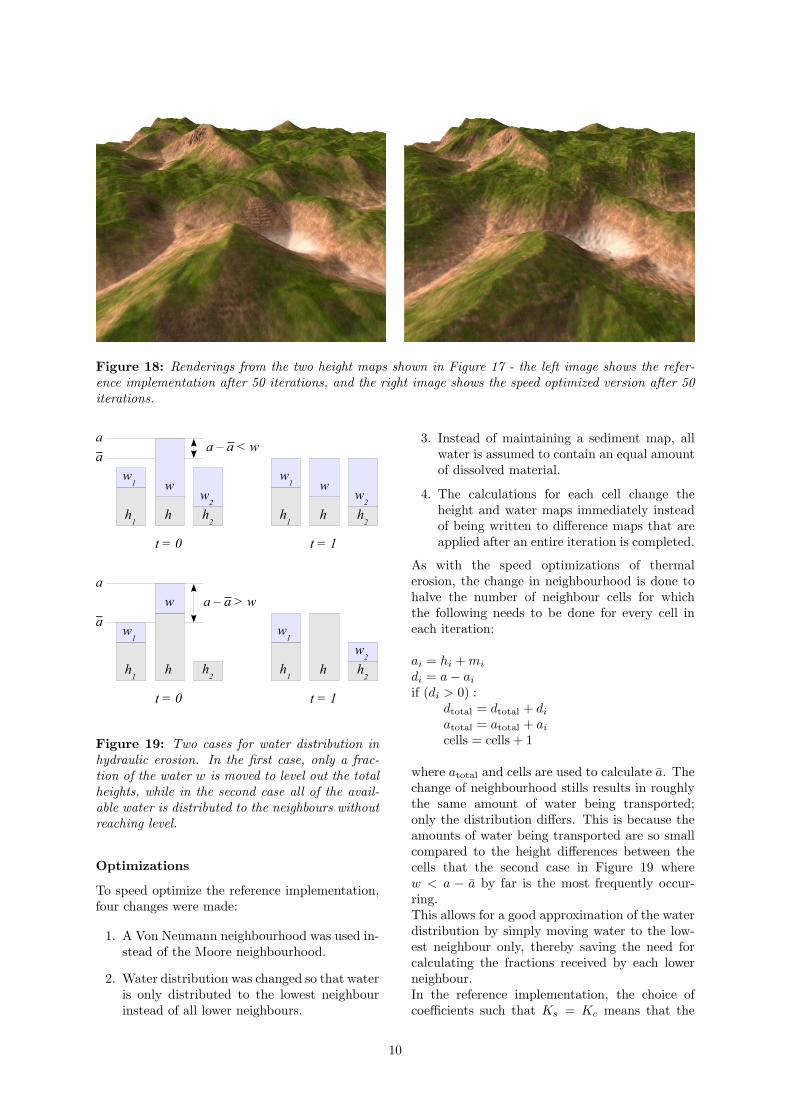
Figure 18: Renderings from the two height maps shown in Figure 17 - the left image shows the refer-ence implementation after 50 iterations, and the right image shows the speed optimized version after 50iterations.

t = 0

t = 0

t = 1

t = 1

a

a

h1

h1

h1

h1

h2

h2

h2

h2

h h

h h

w

w ww

1w

1

w2

w2

w2

a

aa – a < w

a – a > w

w1

w1

Figure 19: Two cases for water distribution inhydraulic erosion. In the first case, only a frac-tion of the water w is moved to level out the totalheights, while in the second case all of the avail-able water is distributed to the neighbours withoutreaching level.

Optimizations

To speed optimize the reference implementation,four changes were made:

1. A Von Neumann neighbourhood was used in-stead of the Moore neighbourhood.

2. Water distribution was changed so that wateris only distributed to the lowest neighbourinstead of all lower neighbours.

3. Instead of maintaining a sediment map, allwater is assumed to contain an equal amountof dissolved material.

4. The calculations for each cell change theheight and water maps immediately insteadof being written to difference maps that areapplied after an entire iteration is completed.

As with the speed optimizations of thermalerosion, the change in neighbourhood is done tohalve the number of neighbour cells for whichthe following needs to be done for every cell ineach iteration:

ai = hi + mi

di = a− ai

if (di > 0) :dtotal = dtotal + di

atotal = atotal + ai

cells = cells + 1

where atotal and cells are used to calculate a. Thechange of neighbourhood stills results in roughlythe same amount of water being transported;only the distribution differs. This is because theamounts of water being transported are so smallcompared to the height differences between thecells that the second case in Figure 19 wherew < a − a by far is the most frequently occur-ring.This allows for a good approximation of the waterdistribution by simply moving water to the low-est neighbour only, thereby saving the need forcalculating the fractions received by each lowerneighbour.In the reference implementation, the choice ofcoefficients such that Ks = Kc means that the

10

amount of material dissolved per water equals thetransport capacity of the water. This causes allthe water to always be at maximum sediment sat-uration: Any water evaporation is immediatelyfollowed by sedimentation of the material that ex-ceeds the transport capacity. Since m = Kc × wfor every cell, there is no need to maintain a sep-arate sediment map. Even with Kc < Ks this is agood approximation, since w drops exponentiallywhich means that maximum saturation is reachedvery quickly.To limit reads and writes to the height and wa-ter maps further, all changes are written directlyinstead of using difference maps that are appliedonly after the entire iteration has been completed.

Analysis

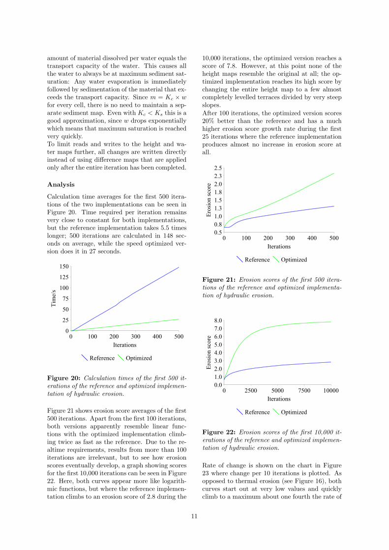
Calculation time averages for the first 500 itera-tions of the two implementations can be seen inFigure 20. Time required per iteration remainsvery close to constant for both implementations,but the reference implementation takes 5.5 timeslonger; 500 iterations are calculated in 148 sec-onds on average, while the speed optimized ver-sion does it in 27 seconds.

0 100 200 300 400 5000

25

50

75

100

125

150

Reference Optimized

Iterations

Time/s

Figure 20: Calculation times of the first 500 it-erations of the reference and optimized implemen-tation of hydraulic erosion.

Figure 21 shows erosion score averages of the first500 iterations. Apart from the first 100 iterations,both versions apparently resemble linear func-tions with the optimized implementation climb-ing twice as fast as the reference. Due to the re-altime requirements, results from more than 100iterations are irrelevant, but to see how erosionscores eventually develop, a graph showing scoresfor the first 10,000 iterations can be seen in Figure22. Here, both curves appear more like logarith-mic functions, but where the reference implemen-tation climbs to an erosion score of 2.8 during the

10,000 iterations, the optimized version reaches ascore of 7.8. However, at this point none of theheight maps resemble the original at all; the op-timized implementation reaches its high score bychanging the entire height map to a few almostcompletely levelled terraces divided by very steepslopes.After 100 iterations, the optimized version scores20% better than the reference and has a muchhigher erosion score growth rate during the first25 iterations where the reference implementationproduces almost no increase in erosion score atall.

0 100 200 300 400 5000.50.81.01.31.51.82.02.32.5

Reference Optimized

Iterations

Ero

sion

sco

re

Figure 21: Erosion scores of the first 500 itera-tions of the reference and optimized implementa-tion of hydraulic erosion.

0 2500 5000 7500 100000.01.02.03.04.05.06.07.08.0

Reference Optimized

Iterations

Ero

sion

sco

re

Figure 22: Erosion scores of the first 10,000 it-erations of the reference and optimized implemen-tation of hydraulic erosion.

Rate of change is shown on the chart in Figure23 where change per 10 iterations is plotted. Asopposed to thermal erosion (see Figure 16), bothcurves start out at very low values and quicklyclimb to a maximum about one fourth the rate of

11

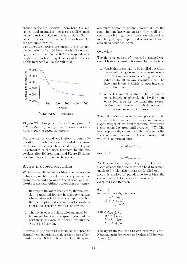
change in thermal erosion. From here, the ref-erence implementation seems to stabilize muchfaster than the optimized version: After 500 it-eration, the rate of change is 3 times higher forthe optimized version.The difference between the outputs of the two im-plementations after 100 iterations is 1% on aver-age, where a difference of 100% corresponds to aheight map with all height values at 0 versus aheight map with all height values at 1.

0 100 200 300 400 5000.0000

0.0004

0.0008

0.0012

0.0016

0.0020

Reference Optimized

Iterations

Cha

nge

per

10 it

erat

ions

Figure 23: Change per 10 iterations of the first500 iterations of the reference and optimized im-plementation of hydraulic erosion.

For practical or visual applications, around 100iterations of both versions are needed to changethe terrain to achieve the desired shape. Figure24 compares height maps produced by the twoversions after 100 iterations, and Figure 25 showsrendered views of these height maps.

A new proposed algorithm

With the overall goal of reaching an erosion scoreas high as possible in as short time as possible, theoptimization and analysis of the thermal and hy-draulic erosion algorithms have shown two things:

1. Because of its low erosion score, thermal ero-sion is unsuited for use in computer gameswhere flatness of the terrain is important, butthe speed optimized version is fast enough tobe used for runtime synthesis of terrain.

2. The effects of hydraulic erosion are much bet-ter suited, but even the speed optimized al-gorithm is too slow to be used for runtimesynthesis of terrain.

To create an algorithm that combines the speed ofthermal erosion with the high erosion score of hy-draulic erosion, it has to be as simple as the speed

optimized version of thermal erosion and at thesame time emulate what causes the hydraulic ero-sion to reach a high score. This was achieved bymodifying the speed optimized version of thermalerosion as described below.

Overview

The high erosion score of the speed optimized ver-sion of hydraulic erosion is caused by two factors:

1. Nearly flat areas tend to be levelled out whenthe water flowing downhill is dispersed over awider area and evaporates, leaving its carriedsediment to fill up any irregularities. Theflattening lowers s which in turn increasesthe erosion score.

2. While the overall height of the terrain re-mains largely unaffected, the levelling outleaves less area for the remaining slopes,making them steeper. This increases σs

which in turn increases the erosion score.

Thermal erosion seems to do the opposite of this:Instead of levelling out flat areas and makingslopes steeper, it distributes material from steepslopes across flat areas until every si,j ≤ T . Thenew proposed algorithm is simply the same as thespeed optimized version of thermal erosion, butwith the conditional check

if (dmax > T )

inverted toif (dmax ≤ T )

As shown in the example in Figure 26, this causesslopes steeper than the talus threshold to remainunaffected while flatter areas are levelled out.Below is a piece of pseudocode describing thecentral part of the algorithm which is run onevery cell each iteration:

dmax = 0for every i in neighbourhood :

di = h− hi

if (di > dmax) :dmax = di

l = iif (0 < dmax ≤ T ) :

∆h = 12dmax

h = h−∆hhl = hl + ∆h

The algorithm was found to work well with a VonNeumann neighbourhood and values of T between8N and 16

N .

12

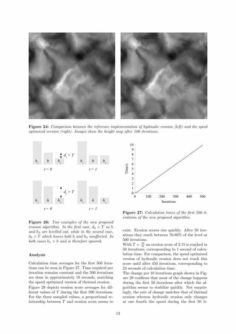
Figure 24: Comparison between the reference implementation of hydraulic erosion (left) and the speedoptimized version (right). Images show the height map after 100 iterations.

t = 0

t = 0

t = 1

t = 1

h1

h1

h1

h1

h2

h2

h2

h2

h h

h h

d2 < T

d2 > T

Figure 26: Two examples of the new proposederosion algorithm. In the first case, d2 < T so hand h2 are levelled out, while in the second case,d2 > T which leaves both h and h2 unaffected. Inboth cases h1 > h and is therefore ignored.

Analysis

Calculation time averages for the first 500 itera-tions can be seen in Figure 27. Time required periteration remains constant and the 500 iterationsare done in approximately 10 seconds, matchingthe speed optimized version of thermal erosion.Figure 28 depicts erosion score averages for dif-ferent values of T during the first 500 iterations.For the three sampled values, a proportional re-lationship between T and erosion score seems to

0 100 200 300 400 500012345678910

Iterations

Time/s

Figure 27: Calculation times of the first 500 it-erations of the new proposed algorithm.

exist. Erosion scores rise quickly: After 50 iter-ations they reach between 70-80% of the level at500 iterations.With T = 16

N an erosion score of 2.15 is reached in50 iterations, corresponding to 1 second of calcu-lation time. For comparison, the speed optimizedversion of hydraulic erosion does not reach thisscore until after 450 iterations, corresponding to24 seconds of calculation time.The change per 10 iterations graph shown in Fig-ure 29 confirms that most of the change happensduring the first 50 iterations after which the al-gorithm seems to stabilize quickly. Not surpris-ingly, the rate of change matches that of thermalerosion whereas hydraulic erosion only changesat one fourth the speed during the first 50 it-

13

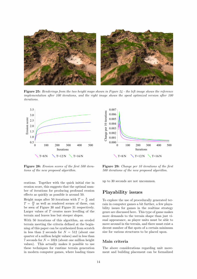
Figure 25: Renderings from the two height maps shown in Figure 24 - the left image shows the referenceimplementation after 100 iterations, and the right image shows the speed optimized version after 100iterations.

0 100 200 300 400 5000.5

1.0

1.5

2.0

2.5

3.0

3.5

T=8/N T=12/N T=16/N

Iterations

Ero

sion

sco

re

Figure 28: Erosion scores of the first 500 itera-tions of the new proposed algorithm.

erations. Together with the quick initial rise inerosion score, this suggests that the optimal num-ber of iterations for producing profound erosioneffects as quickly as possible is around 50.Height maps after 50 iterations with T = 8

N andT = 16

N as well as rendered scenes of these, canbe seen of Figure 30 and Figure 31 respectively.Larger values of T creates more levelling of theterrain and leaves less but steeper slopes.With 50 iterations of this algorithm, an erodedterrain meeting the criteria defined at the begin-ning of this paper can be synthesized from scratchin less than 2 seconds for N = 512 (about onequarter of a million height values) and in less than7 seconds for N = 1024 (about one million heightvalues). This actually makes it possible to usethese techniques for runtime terrain generationin modern computer games, where loading times

0 100 200 300 400 5000.000

0.001

0.002

0.003

0.004

0.005

0.006

0.007

T=8/N T=12/N T=16/N

Iterations

Cha

nge

per

10 it

erat

ions

Figure 29: Change per 10 iterations of the first500 iterations of the new proposed algorithm.

up to 30 seconds are not uncommon.

Playability issues

To explore the use of procedurally generated ter-rain in computer games a bit further, a few playa-bility issues for games in the realtime strategygenre are discussed here. This type of game makesmore demands to the terrain shape than just vi-sual appearance, as player units must be able tomove around in the terrain, and there must exist adecent number of flat spots of a certain minimumsize for various structures to be placed upon.

Main criteria

The above considerations regarding unit move-ment and building placement can be formalized

14

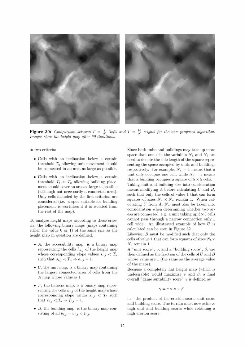
Figure 30: Comparison between T = 8N (left) and T = 16

N (right) for the new proposed algorithm.Images show the height map after 50 iterations.

in two criteria:

• Cells with an inclination below a certainthreshold Tu allowing unit movement shouldbe connected in an area as large as possible.

• Cells with an inclination below a certainthreshold Tb < Tu allowing building place-ment should cover an area as large as possible(although not necessarily a connected area).Only cells included by the first criterion areconsidered (i.e. a spot suitable for buildingplacement is worthless if it is isolated fromthe rest of the map).

To analyse height maps according to these crite-ria, the following binary maps (maps containingeither the value 0 or 1) of the same size as theheight map in question are defined:

• A, the accessibility map, is a binary maprepresenting the cells hi,j of the height mapwhose corresponding slope values si,j < Tu

such that si,j < Tu ⇒ ai,j = 1.

• U , the unit map, is a binary map containingthe largest connected area of cells from theA map whose value is 1.

• F , the flatness map, is a binary map repre-senting the cells hi,j of the height map whosecorresponding slope values si,j < Tb suchthat si,j < Tb ⇒ fi,j = 1.

• B, the building map, is the binary map con-sisting of all bi,j = ui,j × fi,j .

Since both units and buildings may take up morespace than one cell, the variables Nu and Nb areused to denote the side length of the square repre-senting the space occupied by units and buildingsrespectively. For example, Nu = 1 means that aunit only occupies one cell, while Nb = 5 meansthat a building occupies a square of 5× 5 cells.Taking unit and building size into considerationmeans modifying A before calculating U and B,such that only the cells of value 1 that can formsquares of sizes Nu × Nu remain 1. When cal-culating U from A, Nu must also be taken intoconsideration when determining whether two ar-eas are connected, e.g. a unit taking up 3×3 cellscannot pass through a narrow connection only 1cell wide. An illustrated example of how U iscalculated can be seen in Figure 32.Likewise, B must be modified such that only thecells of value 1 that can form squares of sizes Nb×Nb remain 1.A ”unit score”, υ, and a ”building score”, β, arethen defined as the fraction of the cells of U and Bwhose value are 1 (the same as the average valueof the maps).Because a completely flat height map (which isundesirable) would maximize υ and β, a finaloverall ”game suitability score” γ is defined as

γ = ε× υ × β

i.e. the product of the erosion score, unit scoreand building score. The terrain must now achievehigh unit and building scores while retaining ahigh erosion score.

15

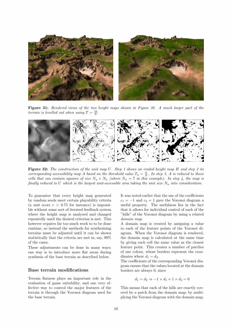
Figure 31: Rendered views of the two height maps shown in Figure 30. A much larger part of theterrain is levelled out when using T = 16

N .

Figure 32: The construction of the unit map U . Step 1 shows an eroded height map H and step 2 itscorresponding accessibility map A based on the threshold value Tu = 8

N . In step 3, A is reduced to thosecells that can contain squares of size Nu × Nu (where Nu = 7 in this example). In step 4, the map isfinally reduced to U which is the largest unit-accessible area taking the unit size Nu into consideration.

To guarantee that every height map generatedby random seeds meet certain playability criteria(a unit score υ > 0.75 for instance) is impossi-ble without some sort of iterated feedback systemwhere the height map is analyzed and changedrepeatedly until the desired criterion is met. Thishowever requires far too much work to to be doneruntime, so instead the methods for synthesizingterrains must be adjusted until it can be shownstatistically that the criteria are met in, say, 99%of the cases.These adjustments can be done in many ways;one way is to introduce more flat areas duringsynthesis of the base terrain as described below.

Base terrain modifications

Terrain flatness plays an important role in theevaluation of game suitability, and one very ef-fective way to control the major features of theterrain is through the Voronoi diagram used forthe base terrain.

It was noted earlier that the use of the coefficientsc1 = −1 and c2 = 1 gave the Voronoi diagram auseful property. The usefulness lies in the factthat it allows for individual control of each of the”hills” of the Voronoi diagram by using a relateddomain map.A domain map is created by assigning a valueto each of the feature points of the Voronoi di-agram. When the Voronoi diagram is rendered,the domain map is calculated at the same timeby giving each cell the same value as the closestfeature point. This creates a number of patchesof one colour, whose borders represent the coor-dinates where d1 = d2.The coefficients of the corresponding Voronoi dia-gram ensure that the values located at the domainborders are always 0, since

d1 = d2 ⇒ −1× d1 + 1× d2 = 0

This means that each of the hills are exactly cov-ered by a patch from the domain map; by multi-plying the Voronoi diagram with the domain map,

16

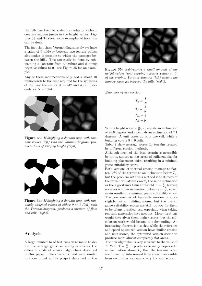
the hills can then be scaled individually withoutcreating sudden jumps in the height values. Fig-ures 33 and 34 show some examples of how thiscan be done.The fact that these Voronoi diagrams always havea value of 0 midway between two feature pointsalso makes it possible to widen the passages be-tween the hills. This can easily be done by sub-tracting a constant from all values and clippingnegative values to 0 - see Figure 35 for an exam-ple.Any of these modifications only add a about 10milliseconds to the time required for the synthesisof the base terrain for N = 512 and 40 millisec-onds for N = 1024.

Figure 33: Multiplying a domain map with ran-dom values (left) with the Voronoi diagram, pro-duces hills of varying height (right).

Figure 34: Multiplying a domain map with ran-domly assigned values of either 0 or 1 (left) withthe Voronoi diagram, produces a mixture of flatsand hills (right).

Analysis

A large number to of test runs were made to de-termine average game suitability scores for thedifferent kinds of erosion algorithms describedin this paper. The constants used were similarto those found in the project described in the

Figure 35: Subtracting a small amount of theheight values (and clipping negative values to 0)of the original Voronoi diagram (left) widens thenarrow passages between the hills (right).

Examples of use section:

Tu =8N

Tb =2N

Nu = 1Nb = 9

With a height scale of N16 , Tu equals an inclination

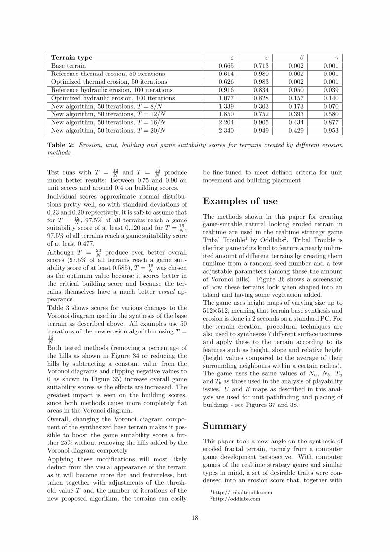
of 26.6 degrees and Tb equals an inclination of 7.1degrees. A unit takes up only one cell, while abuilding covers 9× 9 cells.Table 2 show average scores for terrains createdby different erosion methods.Although most of the base terrain is accessibleby units, almost no flat areas of sufficient size forbuilding placement exist, resulting in a minimalgame suitability score.Both versions of thermal erosion manage to flat-ten 98% of the terrain to an inclination below Tu,but the problem with this method is that most ofthe terrain will attain exactly the same inclinationas the algorithm’s talus threshold T = 4

N , leavingno areas with an inclination below Tb = 2

N , whichagain results in a minimal game suitability score.The two versions of hydraulic erosion produceslightly better building scores, but the overallgame suitability scores are still too low for themto be of any practical use, especially when takingrealtime generation into account. More iterationswould have given them higher scores, but the cal-culation work would become too demanding. Aninteresting observation is that while the referenceand speed optimized version have similar erosionand unit scores, the optimized version seems toproduce more almost completely flat areas.The new algorithm is very sensitive to the value ofT . With T = 8

N , it produces so many slopes withan inclination above Tu that the terrains oftenare broken up into several large areas inaccessiblefrom each other, causing a very low unit score.

17

Terrain type ε υ β γBase terrain 0.665 0.713 0.002 0.001Reference thermal erosion, 50 iterations 0.614 0.980 0.002 0.001Optimized thermal erosion, 50 iterations 0.626 0.983 0.002 0.001Reference hydraulic erosion, 100 iterations 0.916 0.834 0.050 0.039Optimized hydraulic erosion, 100 iterations 1.077 0.828 0.157 0.140New algorithm, 50 iterations, T = 8/N 1.339 0.303 0.173 0.070New algorithm, 50 iterations, T = 12/N 1.850 0.752 0.393 0.580New algorithm, 50 iterations, T = 16/N 2.204 0.905 0.434 0.877New algorithm, 50 iterations, T = 20/N 2.340 0.949 0.429 0.953

Table 2: Erosion, unit, building and game suitability scores for terrains created by different erosionmethods.

Test runs with T = 12N and T = 16

N producemuch better results: Between 0.75 and 0.90 onunit scores and around 0.4 on building scores.Individual scores approximate normal distribu-tions pretty well, so with standard deviations of0.23 and 0.20 repsectively, it is safe to assume thatfor T = 12

N , 97.5% of all terrains reach a gamesuitability score of at least 0.120 and for T = 16

N ,97.5% of all terrains reach a game suitability scoreof at least 0.477.Although T = 20

N produce even better overallscores (97.5% of all terrains reach a game suit-ability score of at least 0.585), T = 16

N was chosenas the optimum value because it scores better inthe critical building score and because the ter-rains themselves have a much better visual ap-pearance.Table 3 shows scores for various changes to theVoronoi diagram used in the synthesis of the baseterrain as described above. All examples use 50iterations of the new erosion algorithm using T =16N .Both tested methods (removing a percentage ofthe hills as shown in Figure 34 or reducing thehills by subtracting a constant value from theVoronoi diagrams and clipping negative values to0 as shown in Figure 35) increase overall gamesuitability scores as the effects are increased. Thegreatest impact is seen on the building scores,since both methods cause more completely flatareas in the Voronoi diagram.Overall, changing the Voronoi diagram compo-nent of the synthesized base terrain makes it pos-sible to boost the game suitability score a fur-ther 25% without removing the hills added by theVoronoi diagram completely.Applying these modifications will most likelydeduct from the visual appearance of the terrainas it will become more flat and featureless, buttaken together with adjustments of the thresh-old value T and the number of iterations of thenew proposed algorithm, the terrains can easily

be fine-tuned to meet defined criteria for unitmovement and building placement.

Examples of use

The methods shown in this paper for creatinggame-suitable natural looking eroded terrain inrealtime are used in the realtime strategy gameTribal Trouble1 by Oddlabs2. Tribal Trouble isthe first game of its kind to feature a nearly unlim-ited amount of different terrains by creating themruntime from a random seed number and a fewadjustable parameters (among these the amountof Voronoi hills). Figure 36 shows a screenshotof how these terrains look when shaped into anisland and having some vegetation added.The game uses height maps of varying size up to512×512, meaning that terrain base synthesis anderosion is done in 2 seconds on a standard PC. Forthe terrain creation, procedural techniques arealso used to synthesize 7 different surface texturesand apply these to the terrain according to itsfeatures such as height, slope and relative height(height values compared to the average of theirsurrounding neighbours within a certain radius).The game uses the same values of Nu, Nb, Tu

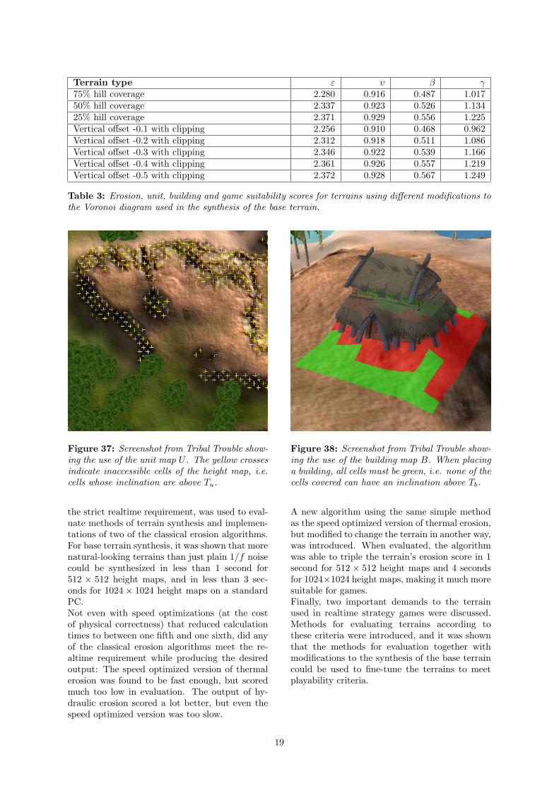
and Tb as those used in the analysis of playabilityissues. U and B maps as described in this anal-ysis are used for unit pathfinding and placing ofbuildings - see Figures 37 and 38.

Summary

This paper took a new angle on the synthesis oferoded fractal terrain, namely from a computergame development perspective. With computergames of the realtime strategy genre and similartypes in mind, a set of desirable traits were con-densed into an erosion score that, together with

1http://tribaltrouble.com2http://oddlabs.com

18

Terrain type ε υ β γ75% hill coverage 2.280 0.916 0.487 1.01750% hill coverage 2.337 0.923 0.526 1.13425% hill coverage 2.371 0.929 0.556 1.225Vertical offset -0.1 with clipping 2.256 0.910 0.468 0.962Vertical offset -0.2 with clipping 2.312 0.918 0.511 1.086Vertical offset -0.3 with clipping 2.346 0.922 0.539 1.166Vertical offset -0.4 with clipping 2.361 0.926 0.557 1.219Vertical offset -0.5 with clipping 2.372 0.928 0.567 1.249

Table 3: Erosion, unit, building and game suitability scores for terrains using different modifications tothe Voronoi diagram used in the synthesis of the base terrain.

Figure 37: Screenshot from Tribal Trouble show-ing the use of the unit map U . The yellow crossesindicate inaccessible cells of the height map, i.e.cells whose inclination are above Tu.

the strict realtime requirement, was used to eval-uate methods of terrain synthesis and implemen-tations of two of the classical erosion algorithms.For base terrain synthesis, it was shown that morenatural-looking terrains than just plain 1/f noisecould be synthesized in less than 1 second for512 × 512 height maps, and in less than 3 sec-onds for 1024 × 1024 height maps on a standardPC.Not even with speed optimizations (at the costof physical correctness) that reduced calculationtimes to between one fifth and one sixth, did anyof the classical erosion algorithms meet the re-altime requirement while producing the desiredoutput: The speed optimized version of thermalerosion was found to be fast enough, but scoredmuch too low in evaluation. The output of hy-draulic erosion scored a lot better, but even thespeed optimized version was too slow.

Figure 38: Screenshot from Tribal Trouble show-ing the use of the building map B. When placinga building, all cells must be green, i.e. none of thecells covered can have an inclination above Tb.

A new algorithm using the same simple methodas the speed optimized version of thermal erosion,but modified to change the terrain in another way,was introduced. When evaluated, the algorithmwas able to triple the terrain’s erosion score in 1second for 512 × 512 height maps and 4 secondsfor 1024×1024 height maps, making it much moresuitable for games.Finally, two important demands to the terrainused in realtime strategy games were discussed.Methods for evaluating terrains according tothese criteria were introduced, and it was shownthat the methods for evaluation together withmodifications to the synthesis of the base terraincould be used to fine-tune the terrains to meetplayability criteria.

19

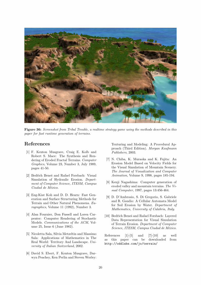
Figure 36: Screenshot from Tribal Trouble, a realtime strategy game using the methods described in thispaper for fast runtime generation of terrains.

References

[1] F. Kenton Musgrave, Craig E. Kolb andRobert S. Mace: The Synthesis and Ren-dering of Eroded Fractal Terrains. ComputerGraphics, Volume 23, Number 3, July 1989,pages 41-50.

[2] Bedrich Benes and Rafael Forsbach: VisualSimulation of Hydraulic Erosion. Depart-ment of Computer Science, ITESM, CampusCiudad de Mexico.

[3] Eng-Kiat Koh and D. D. Hearn: Fast Gen-eration and Surface Structuring Methods forTerrain and Other Natural Phenomena. Eu-rographics, Volume 11 (1992), Number 3.

[4] Alan Fournier, Don Fussell and Loren Car-penter: Computer Rendering of StochasticModels. Communications of the ACM, Vol-ume 25, Issue 6 (June 1982).

[5] Nicoletta Sala, Silvia Metzeltin and MassimoSala: Applications of Mathematics in TheReal World: Territory And Landscape. Uni-versity of Italian Switzerland, 2002.

[6] David S. Ebert, F. Kenton Musgrave, Dar-wyn Peachey, Ken Perlin and Steven Worley:

Texturing and Modeling: A Procedural Ap-proach (Third Edition). Morgan KaufmannPublishers, 2003.

[7] N. Chiba, K. Muraoka and K. Fujita: AnErosion Model Based on Velocity Fields forthe Visual Simulation of Mountain Scenery.The Journal of Visualization and ComputerAnimation, Volume 9, 1998, pages 185-194.

[8] Kenji Nagashima: Computer generation oferoded valley and mountain terrains. The Vi-sual Computer, 1997, pages 13:456-464.

[9] D. D’Ambrosio, S. Di Gregorio, S. Gabrieleand R. Gaudio: A Cellular Automata Modelfor Soil Erosion by Water. Department ofMathematics, University of Calabria, Italy.

[10] Bedrich Benes and Rafael Forsbach: LayeredData Representation for Visual Simulationof Terrain Erosion. Department of ComputerScience, ITESM, Campus Ciudad de Mexico.

References [1]-[5] and [7]-[10] as wellas this paper can be downloaded fromhttp://oddlabs.com/jo/terrain/

20