Realtime On-Road Vehicle Detection withOptical Flows and Haar-like feature detectors

Jaesik ChoiDepartment of Computer Science

University of Illinois at Urbana-ChampaignUrbana, IL 61801

jaesik@illinois.edu

Abstract

The autonomous vehicle system is a demanding applica-tion for our daily life. The vehicle requires on-road vehicledetection algorithms. Given the sequence of images, thealgorithms need to find on-road vehicles in realtime. Basi-cally there are two types of on-road vehicles, either travel-ing in the opposite direction or traveling in the same direc-tion. Due to the distinct features of two types of vehicles,different approaches are necessary to detect each direction.Here, we suggest the ‘optical flow’ to detect the coming traf-fics because the coming traffics represent distinct motion.We use ‘Haar-like feature detection’ for the traffics in thesame direction because the traffics represent relatively sta-ble shape (car rear) and little motion. We verify the detectedregion with estimating 3D geometry. If the detectors fail tofind the vehicles, we interpolate the region from the previ-ous frames. Then, the detected vehicles are projected intothe 3D space. Our system detects vehicles with high accu-racy and realtime for 11 frames/sec.

1. IntroductionA vehicle detection algorithm is one of the most im-

portant modules of an autonomous vehicle system becauseit detects midrange and long distance (over 20m) vehicleswith low cost. However, any vehicle detection algorithmcan not detect all vehicles. Here, we consider detectingtwo types of cars. The two types of cars (traveling in theopposite direction and in the same direction) have distinctfeatures.

We use ‘Optical flow’ [5] to detect coming traffics.Given the two consecutive frames, we find corner pointswith corner detector [7]. The detected features are matchedby the ‘Optical flow’ algorithm [5]. The ‘Optical flow’ as-sumes that important features are detected in both frames.We cluster some features into a rectangle if the euclidian

distance of two features (the location of feature and thedirection of optical flow) are small. The optical flow al-gorithms find the correspondence within a reasonable timeso that we can use the algorithms for realtime application1. However, some of optical flows are generated by somecracks of the road and road signs. They make false positiverectangles.

Haar-like feature detector [11] is used to detect trafficsin the same direction. The optical flow algorithm is not soappropriate for these traffics because they do not have anysalient movement in most case. Instead, they maintain someconsistent shapes. The shapes mostly show the rear side ofthe car. To detect the rear shape of the car we choose to useHaar-like feature detector because it is fast and efficient. Ingeneral, template-based methods are slow for realtime de-tections. The execution time of the methods is proportionalto the number of templates we have. That is, the executiontime increases when we have more templates. However,Haar-like feature detector searches the frame once. The de-tector also generates many false positives because the detec-tor represents the various shapes of the vehicles. If we onlyfocus on the shapes of the cars in the training data set, thedetector easily finds those cars. However, the detector mayfail to find the cars which are not trained. It is dangerous forthe autonomous vehicle. Thus, we loosen the constraints ofthe detector and receive some false positive detections.

Many false positive rectangles (or detections) can be fil-tered out, when we process the image based on the contextof the scene [4]. We estimate 3D geometry and use it toimpose the constraints of geometry. If we find a vanishingpoint in a frame, the rectangle (hypothesis) can be verifiedby its size. We assume that the sizes of cars are in certainranges. If the cars locate near the vanishing point, the sizes

1real-time is a different term with the term in real-time operating sys-tem. The real-time in the operating system means that the system alwaysfinish its works within appointed time. Here, the real-time in some papersmeans that the processing time of vehicle tracking is faster than the framerate. That is, there is no guarantee to meet the dead line

should be small. If the cars are far from the vanishing point,the sizes should not so small. Of course, any car can not beon the sky. With this simple method, we filtered out mayfalse positive detections.

Although there are many researches for realtime on-roadvehicle detection [1, 9, 13] so far, there is no research thatuse Haar-like feature detector, optical flow and scene con-text simultaneously on the moving vehicle with monocularcamera. Recently some researchers [8], [12] have improvedthe performance of Viola’s detector. Miolos [8] reducedthe time for training parameters and Jianyu [12] focused onimproving the tracking performance with particle filtering.However, those are not designed for real-time detection ofon-road vehicles.

In general, a vehicle detection algorithm has two basicstep; Hypothesis Generation (HG) and Hypothesis Verifi-cation (HV) [6]. In the Hypothesis Generation (HG) step,the algorithm hypothesizes the locations of vehicles in animage. In the Hypothesis Verification (HV) step, the algo-rithm verify the presence of vehicles in an image. The meth-ods in the HG step can be categorized into three methods;Knowledge-based methods using symmetry of object, color,corners and edges; Stereo-Vision-Based methods using twocameras; Motion-Based Methods tracking the motion ofpixels between the consecutive frames (optical flow[5]).The methods in the HV step are Template-based methodsand Appearance methods. Template-based methods usepredefined patterns of the vehicle class. Appearance-basedmethods include pattern classification system between ve-hicle and non-vehicle.

Three previous works [1, 9, 13] tried to solve realtimeon-road vehicle detection problem. All the papers usedmonocular cameras and have real-time constraints. [1] usedhorizontal and vertical edges (Knowledge-based methods)in HG step. The selected regions at HG step are matchedwith predefined templates in HV step. [9] used horizon-tal and vertical edge in HG step. However, they use HaarWavelet Transform and SVMs (Appearance-based meth-ods) in HV step. [13] detected long-distance stationary ob-stacles including vehicles. They used an efficient opticalflow algorithm [3] (Motion-based methods) in HG step. Al-though they did not use any traditional HV method, theyused Sum of squared differences(SSD) with a thresholdvalue to verify their hypothesis.

2. Theories

This works use three prevail methods in computer vision.They are ‘optical flow’ [5], ‘Haar-like feature detector’ [11](so-called Viola and Jones), and ‘Scene analysis with con-text’ [4]. A normalized input image is simultaneously pro-cessed by ‘optical flow’ and ‘Viola and Jones detector’. Thehypothesis are analyzed by ‘Scene analysis with context’.

Input Image

Cars traveling in the same direction

Haar-like Feature Detector

Kalman Filter (DBN) & Projection into 3D image

Cars traveling in the opposite direction

Corner detector & Optical Flow

Viewpoint filteringEstimate 3D geometry using vanishing point

Figure 1: Overall diagram of on-road vehicle detection algorithms.

2.1. Optical Flow

Overall process of optical is following: First, the algo-rithm finds the important features (corners) in the two con-secutive frames; Second, the algorithm matches the corre-spondence between the features (corners); Finally, extractedflows are clustered into a group if the Euclidean distancesof the flows (location and direction) are small.

2.1.1 Detecting Corner Features

We use Shi and Tomasi [7] corner detector that is modifiedfrom the Harris corner detector. The Shi corner detectorassume the motion can be modeled by Affine, and the mo-tion is small. The assumption is reasonable for this researchbecause we have enough frame rates (15 frames/sec) so thatthe movement of vehicles is bounded by small range. Giventhe image patch over the area (u, v), Harris corner detectorfind corner with shifting it by (x, y). The SSD betweenthese two patches, S is given by

S =∑u

∑v

(I(u, v)− I(u− x, v − y))2

When I is the intensity of image a position (eg. u,v ).The Harris matrix is found by taking the second derivativeof S around (x,y) = (0,0). A is given by

A =

∣∣∣∣ I2x IxIyIxIy I2y

∣∣∣∣The strength of the corner is determined by ‘how much’second derivative there is. The two eigenvalues (λ1 and λ2)of A can be used to detect the corner. If the two eigenvaluesare large, distinct positive value, the a corner is found.

Shi and Tomasi [7] corner detector based on the Har-ris corner detector. Instead of simple translation, they use

Affine transformation. Given the image patch over the area(u, v), Shi and Tomasi corner detector find corner with ap-plying Affine transformation(A) and shifting it by (x,y).

S =∑u

∑v

(I(u, v)− I(A(u, v)− (x, y)))2

We have a 6 by 6 matrix because Affine and transformationhave six variables. We find the corner, if the 6 by 6 matrixhave large eigenvalues.

2.1.2 Extracting Optical Flow

Lucas and Kanades optical flow [5] is used to match thefeature points. Given point (u, v) in image It the algorithmfinds the point (u+dx, v+dy) in image It+1 that minimizese,

e(dx, dy) =

u+w∑x=u−w

v+w∑y=v−w

(I(x, y)− I(x+ dx, y + dy))

2.1.3 Clustering into the Groups

We cluster a set of flows into a group, if the flows havesimilar direction and close location. A flow (op) has fourfeatures (x, y, vx, vy) (x, y are the location of the flow; vxand vy are the direction of the flow). Given the two vectorsof optical flows op1(x′, y′, v′x, v

′y) and op2(x′′, y′′, v′′x , v

′′y ),

Euclidean distance(dist(op1, op2)) is defined by follow-ing.√

(x′ − x′′)2 + (y′ − y′′)2 + (vx′ − vx′′)2 + (vy′ − vy′′)2

We design simple nearest neighbor clustering algorithm.Given the a flow (opi), find the closest flow (opj). If thedist(opi, opj) is less than a threshold value θdist, group theopi and opj into same group. If the case when the opj isalready included in a group G′, insert opi into the group G′

(opj ∈ G′ =⇒ opi ∈ G′).If our camera is mounted in the static ground, there is

no additional problem to use the optical flow and this near-est neighbor clustering. All the flows have some biased di-rection in some case, because our camera is also moving.Whenever there is any gap on the road, the camera has solarge movement that the next image has large translation.To prevent this ‘bump it out’ effect, we find the commonbiased vector biasedv(vbx, vby) if there is. Thus an opticalflow (opi(x, y, vx, vy)) has new flow (op′i) as following.

op′i = (x, y, vx − vbx, vy − vby)

2.2. Haar-like Feature Detector

We use Haar-like feature detector and AdaBoost to de-tect the cars in the same direction. Recently Viola and Jones[10, 11] suggest AdaBoost into computer vision. The ap-proach prevails in the face detection because their methodis fast and accurate.

Figure 3: Haar wavelet features are used in this research. A Haar-likefeature is defined by one of above rectangle (or variations) and a thresholdvalue. Given an image I , the sum of intensity of dark region and brightregion are calculated. If the sum of intensity on the dark region is greater(or less) than the sum of intensity on the bright region by the threshold,the region is determined as positive example. Otherwise, the region isdetermined as negative example.

2.2.1 Haar-like Feature

We use three kinds of Haar feature as in figure 3.Denote the feature set as F = fi|i = 1, ..., N and cor-responding feature values on images observation z asV (z) = vi(z)|i = 1, ..., N

The number of features even in a 24 by 24 image patchare so huge to calculate them every time. However, we mayeasily calculate them if we have an accumulated sum of in-tensity from origin.

Sacc(i, j) =

i∑x=0

j∑y=0

I(i, j)

If a rectangle is defined by the region ( [xleft, xright] ×[yup, ydown], the sum of intensity in the rectangle is as fol-lowing,

Sacc(xright, ydown)− Sacc(xleft, ydown)

−Sacc(xright, yup) + Sacc(xleft, yup)

2.2.2 Learning with AdaBoost

A Haar-like feature is a classifier because a feature can clas-sify the whole group of images into positive image and neg-ative ones. We use the Haar-like feature as a weak classifierof AdaBoost algorithm, as the Viola and Jones did it forface detection. Even if a feature satisfies a simple criteria(the error ratio is less than a guess (0.5) ), we can use the

1 2 3

4 5 6

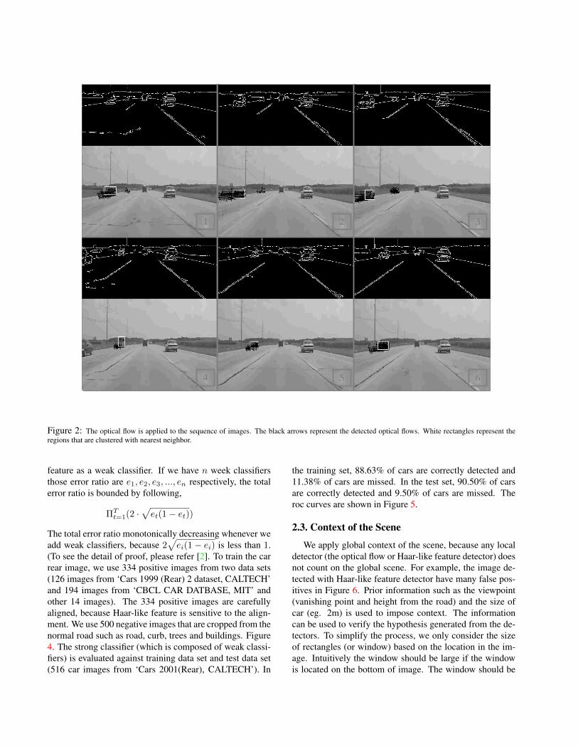
Figure 2: The optical flow is applied to the sequence of images. The black arrows represent the detected optical flows. White rectangles represent theregions that are clustered with nearest neighbor.

feature as a weak classifier. If we have n week classifiersthose error ratio are e1, e2, e3, ..., en respectively, the totalerror ratio is bounded by following,

ΠTt=1(2 ·

√et(1− et))

The total error ratio monotonically decreasing whenever weadd weak classifiers, because 2

√ei(1− ei) is less than 1.

(To see the detail of proof, please refer [2]. To train the carrear image, we use 334 positive images from two data sets(126 images from ‘Cars 1999 (Rear) 2 dataset, CALTECH’and 194 images from ‘CBCL CAR DATBASE, MIT’ andother 14 images). The 334 positive images are carefullyaligned, because Haar-like feature is sensitive to the align-ment. We use 500 negative images that are cropped from thenormal road such as road, curb, trees and buildings. Figure4. The strong classifier (which is composed of weak classi-fiers) is evaluated against training data set and test data set(516 car images from ‘Cars 2001(Rear), CALTECH’). In

the training set, 88.63% of cars are correctly detected and11.38% of cars are missed. In the test set, 90.50% of carsare correctly detected and 9.50% of cars are missed. Theroc curves are shown in Figure 5.

2.3. Context of the Scene

We apply global context of the scene, because any localdetector (the optical flow or Haar-like feature detector) doesnot count on the global scene. For example, the image de-tected with Haar-like feature detector have many false pos-itives in Figure 6. Prior information such as the viewpoint(vanishing point and height from the road) and the size ofcar (eg. 2m) is used to impose context. The informationcan be used to verify the hypothesis generated from the de-tectors. To simplify the process, we only consider the sizeof rectangles (or window) based on the location in the im-age. Intuitively the window should be large if the windowis located on the bottom of image. The window should be

Figure 4: Three of detected Haar-like features are shown atthe upper side of figure. Three of sample images are show atthe bottom of figure. The leftmost detected feature detectsthe shadow of car. Other two features show the right edgeand left edge of cars.

ROC curve for training data ROC curve for test data

Figure 5: Left graph shows the roc curve for the test dataset. Right graph shows the roc curve for the training dataset.

small if the window is near the vanishing point. Moreover,there is no window for the car above the vanishing point.The vanishing point (vpx, vpy) is found by Hough trans-form. If the bottom of a rectangle is on the y = yheight,the size of rectangle is proportional to the yheight − vpy(when yheight > vpy). We estimate the probability of sizeof window based on the location as following,

P (Windowsize|x, y) = P (Windowsize|y − vpy)

If the probability of a hypotheses (rectangle) is so small, wereject the rectangles.

3. Technical DetailsTo find the location of the vehicles in the 3D space, we

also use other methods. We improve our tracking perfor-mance with interpolation between the frames. The Kalman

Figure 6: The red rectangles are the regions that are detectedby the Haar-like feature detector. The detector finds the lo-cation of cars in some case (true positive). However, thereare still many false positive rectangles. Some of small rect-angles (false positive) can be rejected based on the globalcontext of scene, because we know that the viewpoint andthe size of car.

filter is used to smooth the tracking process. The rectanglesin the image are mapped onto the 3D geometry.

3.1. Filtering from Multiple Frames

Not only the optical flow but also Haar-like feature de-tector has many false positives. If we reduce the number offalse positive, we also miss many true positives. We cannotrestrict number of false positives, because it is very danger-ous to have many true negatives. To solve this problem, wemaintain the history of detections. We define a flag functionas following,

O(x, y)t = 1 x, y is in any detected rectangle at time tO(x, y)t = 0 otherwise

At time step k, we can lookup the previous n frames. Weregard a point has high probability of detection, if a point(x,y) is occupied by any rectangles recently. (n ∗ f of nframes).

P (carx,y|k,O(.))k = 1 if

n∑i=k−n+1

O(x, y)i > n ∗ f

P (carx,y|k,O(.))k = 0 otherwise

Given the rectangle [x1, x2] × [y1, y2], we verify the rect-angle as a car, if the number of points determined as a carare greater than a certain ratio (eg. 80%). Otherwise, wereject it. The white region in the Figure 8 shows the regionsthat have P (carx,y|.)k = 1.

Δ θθ h

dist = h * tan( θ+ n *∆θ )

Figure 7: Detected car is mapped onto the 3D space

3.2. The Kalman filter

The detectors do not always work well. That is, a car de-tected in time t is not be detected in time t+1. It is becausethe Viola and Jones detector is sensitive to the alignment.However we cannot examine all the possible windows, be-cause it takes so long time to prevent realtime image pro-cessing. Especially, the detector often misses small cars(long distant one).

To solve this problem, we maintain the list of cars de-tected at the previous time step. All the variables such aslocation, size and velocity are maintained with those confi-dences. If the detectors miss the region, we still generate theregion as a car with low confidence. If the detectors find theregion, we update the value of variables (location, size andvelocity) with high confidence. The Kalman filter is used inthis step. One of functions of Kalman filter is smoothing.We have large noise in our image sequences because we aremoving while tracking other vehicles. Thus, we have manyvariances not only in the input image but also in the outputs.However, we can reduce the noise because we maintain thevariable based on the previous observation.

3.3. Projection into 3D Space

Finally, the detected and verified rectangles are projectedonto the 3D space as the Figure 7.

4. ConclusionWe detect two distinct types of vehicles with ‘optical

flow’ and ‘Haar-like feature detector’. We use two algo-rithms because of the different features between the comingtraffics and the vehicles in the same direction. The ‘opti-cal flow’ is appropriate for the coming traffics because theyhave relatively salient motion. ‘Haar-like feature detector’developed by Viola and Jones is promising to detect the carsin the same direction.

To reduce a number of false positives, we consider thescene context. If we find a vanishing point, we can easilyfilter many false positives out. Moreover, we look up previ-ous n frames to reduce the false positives out. If the area has

Figure 9: A table that shows the time that takes to processeach process. The total time for a frame, it takes 0.168 secs.For the 15 frames, it takes 2.527 secs. However, we mayachieve 0.088 secs for a frame, if exclude I/O (the read/writemovie file). That takes 1.324 secs for the 15 frames.

no evidence detecting a vehicle, the rectangle (hypotheses)will be rejected.

We maintain the list of cars detected at the previous step.Whenever the detectors fail to find the probable vehicles,we interpolate the candidate in the output. Kalman filtermaintain the value and confidence of variables.

We train the Haar-like feature with AdaBoost against334 images brought from two data sets (1999 CALTECH,CBCL MIT). The performance is evaluated against another516 images (2001 CALTECH). We achieve the 88.63% ofaccuracy against test set and 90.50% of accuracy against thetraining set. Figure 5 shows the roc curve of two results.

The system is fast enough to process 11 frames per sec-onds. Although Viola’s detector takes rather longer time, itis scalable when the training data set increases.1 In contrast,template-based methods are not scalable to the number ofmodels.

Therefore, the contribution of this work is two things: (1)building a realtime car detection system based on the Haar-like feature detector (2) reducing a number of false positivesbased on the temporal and spatial context.

References[1] M. Betke, E. Haritaoglu, and L. Davis. Real-time multiple

vehicle detection and tracking from a moving vehicle. MVA,12(2):69–83, 2000. 2

[2] Y. Freund and R. E. Schapire. A decision-theoretic general-ization of on-line learning and an application to boosting. InProceedings of the Second European Conference on Compu-tational Learning Theory, pages 23–37, London, UK, 1995.Springer-Verlag. 4

[3] G. D. Hager and P. N. Belhumeur. Efficient region trackingwith parametric models of geometry and illumination. IEEETransactions on Pattern Analysis and Machine Intelligence,20(10):1025–1039, 1998. 2

1Source codes can be download at‘reason.cs.uiuc.edu/jaesik/projects/Vehicle Detection/Jaesik Choi src.zip‘

1 2 3

4 5 6

Figure 8: Some of frames, which are extracted from the result movie file. Red rectangles show the cars which are detectedby the Viola detector. The blue rectangle is the cars that are detected by the optical flow. White area represents the history ofdetection. That is the area of high probability of cars. Upper right part shows the locations of cars that is mapped onto 3D.

[4] D. Hoiem, A. Efros, and M. Hebert. Putting objects in per-spective. In CVPR, 2006. 1, 2

[5] B. D. Lucas and T. Kanade. An iterative image registrationtechnique with an application to stereo vision. In Proc. of the7th IJCAI, pages 674–679, Vancouver, Canada, 1981. 1, 2, 3

[6] R. Miller. On-road vehicle detection: A review. IEEE Trans.Pattern Anal. Mach. Intell., 28(5):694–711, 2006. Member-Zehang Sun and Member-George Bebis. 2

[7] J. Shi and C. Tomasi. Good features to track. In IEEEConference on Computer Vision and Pattern Recognition(CVPR’94), Seattle, June 1994. 1, 2

[8] M. Stojmenovic. Real time machine learning based car de-tection in images with fast training. Mach. Vision Appl.,17(3):163–172, 2006. 2

[9] Z. Sun, R. Miller, G. Bebis, and D. DiMeo. A real-timeprecrash vehicle detection system. In Proceedings of the2002 IEEE Workshop on Applications of Computer Vision,Orlando, FL, Dec. 2002. 2

[10] P. Viola and M. Jones. Robust real-time object detection.International Journal of Computer Vision - to appear, 2002.3

[11] P. Viola, M. Jones, and D. Snow. Detecting pedestrians usingpatterns of motion and appearance, 2003. 1, 2, 3

[12] J. Wang, X. Chen, and W. Gao. Online selecting discrimi-native tracking features using particle filter. In CVPR ’05:Proceedings of the 2005 IEEE Computer Society Conferenceon Computer Vision and Pattern Recognition (CVPR’05) -

Volume 2, pages 1037–1042, Washington, DC, USA, 2005.IEEE Computer Society. 2

[13] A. Wedel, U. Franke, J. Klappstein, T. Brox, and D. Cre-mers. Realtime depth estimation and obstacle detection frommonocular video. In K. F. et al., editor, Pattern Recogni-tion (Proc. DAGM), volume 4174 of LNCS, pages 475–484,Berlin, Germany, September 2006. Springer. 2