© 2012 Jaesik Choi

LIFTED INFERENCE FOR RELATIONAL HYBRID MODELS

BY

JAESIK CHOI

DISSERTATION

Submitted in partial fulfillment of the requirementsfor the degree of Doctor of Philosophy in Computer Science

in the Graduate College of theUniversity of Illinois at Urbana-Champaign, 2012

Urbana, Illinois

Doctoral Committee:

Associate Professor Eyal Amir, Chair, Director of ResearchProfessor Dan RothProfessor Steven M. LavalleProfessor David Poole, University of British Columbia

UIN: 672212292

CERTIFICATE OFCOMMITTEE ApPROVAL

University ofIllinois at Urbana-Champaign

Graduate College

April 5, 2012

We hereby recommend that the thesis by:

JAESIKCHOI

Entitled:

LIFTED INFERENCE FOR RELATIONAL HYBRID MODELS

Be accepted in partial fulfillment ofthe requirements for the degree of

Committee on Final Examination"

Chairperson ­ Ass .

~~~'\_----Comml/lee Member - Professor Steven M. LaValle

Committee Member ­

Committee Member - Professor David Poole

Committee Member ­

* Required for doctoral degree but not for master's degree

ABSTRACT

Probabilistic Graphical Models (PGMs) promise to play a prominent role in many

complex real-world systems. Probabilistic Relational Graphical Models (PRGMs)

scale the representation and learning of PGMs. Answering questions using PRGMs

enables many current and future applications, such as medical informatics, en-

vironmental engineering, financial forecasting and robot localizations. Scaling

inference algorithms for large models is a key challenge for scaling up current

applications and enabling future ones.

This thesis presents new insights into large-scale probabilistic graphical mod-

els. It provides fresh ideas for maintaining a compact structure when answer-

ing questions or inferences about large, continuous models. The insights result

in a key contribution, the Lifted Relational Kalman filter (LRKF), an efficient

estimation algorithm for large-scale linear dynamic systems. It shows that the

new relational Kalman filter enables scaling the exact vanilla Kalman filter from

1,000 to 1,000,000,000 variables. Another key contribution of this thesis is that

it proves that typically used probabilistic first-order languages, including Markov

Logic Networks (MLNs) and First-Order Probabilistic Models (FOPMs), can be

reduced to compact probabilistic graphical representations under reasonable con-

ditions. Specifically, this thesis shows that aggregate operators and the existential

quantification in the languages are accurately approximated by linear constraints

in the Gaussian distribution. In general, probabilistic first-order languages are

transformed into nonparametric variational models where lifted inference algo-

rithms can efficiently solve inference problems.

ii

To My Loving Family and Trusted Friends.

iii

ACKNOWLEDGMENTS

Fortunately enough, pursuing my Ph.D. degree in Urbana-Champaign was the

happiest time of my life. Inspiring fellow researchers guided my research. My

loving family and trusted friends fully supported me during the studies.

First of all, I deeply appreciate my advisor, Eyal Amir, for his generous sup-

port during my studies. Without him, I may not have been able to work on such

exciting research problems including my thesis topic. His invaulable advice and

guidance were crucial to making progress on this thesis. He always has been a

trustful mentor and has been with me almost like a longtime friend. He often

treated himself as an equal collaborator instead of a supervisor, and encouraged

me to lead the research projects. I appreciate his thoughtful and generous consid-

eration more than I can say.

It was my pleasure to interact closely with Dan Roth during the studies. His

gentle and wise advice helped me several times. His excellent machine learning

courses provided valuable foundations of artificial intelligence. His emphasis on

critical thinking has significantly influenced my research. Also, his constructive

feedback on this thesis greatly helped me plan future work.

I enjoyed discussing my thesis with Steven LaValle. Whenever I visited his

office to get advice on my ideas, he always provided lots of related work without

hesitation. Especially, his suggestions helped me a lot when I worked on robot

planning problems. Also, he shared his candid experience how he came up with

his seminal work, and encouraged me to realize the potentials of my current re-

search work.

I was grateful to discuss with David Poole on my thesis. After Eyal suggested

iv

that I read Davids previous work, I was fascinated with his papers and results.

Also, I was indebted to David because his excellent research work always gave me

exciting new directions to pursue. It was my great pleasure that he recommended

my work to be included in a IJCAI-11 tutorial and agreed to be on my thesis

committee. I deeply appreciate his splendid suggestions on my thesis.

I also want to thank to Gerald Dejong for fruitful discussions on my thesis. His

encouragement of my research toward human level intelligence gave me confi-

dence on writing this thesis. I regret not discussing with him earlier.

In 2010, I spent an enjoyable summer with excellent researchers at SRI Interna-

tional. I appreciate Rodrigo de Salvo Braz and Hung Bui for active and energetic

collaborations, as part of this thesis (Chapter 4) may not have existed without Ro-

drigo and Hung. Also, I thank Tuyen Ngoc Huynh and David Israel for valuable

comments.

During my studies, I had exciting opportunities to work on real-world envi-

ronmental problems. I thank David J. Hill, Yong Liu, Tiangfang Xu and Albert J.

Valocchi for sharing important research problems and collaborating to solve them.

I thank Abner Guzman-Rivera. He has been an intimate friend. His different

perspective stimulated me to advance my ideas. Also, his efforts substantially

improved the writing of Chapter 3. Collaboration with him was very exciting

experience to me. I will never forget the day in Barcelona when we revised the

IJCAI-11 presentation slides all night. Thank you, Abner. I hope your studies go

well, too.

In earlier stages of my studies (just after passing the qualifying exam), I met

Won Jong Jeon and Sang-Chul Lee. We worked together on addressing video

matching problems. The work was not included in this thesis because it is beyond

the scope of this thesis. However, I learned the basics on how to conduct research

from the two fellow researchers.

I also wish to thank the members of my research group, the General Intelli-

gence Group (GIG) or previously the Knowledge Representation and Reasoning

(KRR) Group: Hannaneh Hajishirzi, Afsaneh Shirazi, Mark Richards, Deepak

v

Ramanchandran, Tsvi Achler, Wen Pu, Juan Mancilla Caceres, Codruta Girlea,

and Dafna Shahaf. They gave valuable comments on my research which helped

improve my thesis. I also appreciate valuable comments given by friends in

other artificial intelligence groups: Duan Tran, Ming-Wei Chang, Vivek Sriku-

mar, Alexander Sorokin, Quang Do, Leonardo Bobadilla, and Varsha Hedau.

Throughout my studies, my department staff was very supportive and kind to

me. I want to give special thanks to Donna Coleman, Mary Beth Kelley, and Keely

Ashman.

My trusted friends continuously encouraged me to complete this thesis. Es-

pecially, I want to thank Ikkjin Ahn, Donghwan Jeon, Heeseok Kim, Jeongkeun

Lee, Daehyun Yoon, and their families for listening to my stories and sharing their

wisdom from the beginning of my Ph.D. studies.

Since I arrived at Urbana-Champaign, many Korean friends helped me settle

down and gave me valuable feedback when I prepared important milestones in-

cluding the qualifying exam, the preliminary exam and the thesis defense. I deeply

appreciate them: Hyunsu Ju, Bongki Kim, Youngha Kim, Dongyun Jin, Eunsoo

Seo, Sangkyum Kim, Steve Ko, Kihwal Lee, Jin Heo, Jungmin So, Wonson Ahn,

Younhee Ko, Sungjin Im, MyungJoo Ham, Yoonkyong Lee, YoungMin Kwon,

Han-Ul Yoon, Jihyuk Choi, Wucherl Yoo, Hyun Duk Kim, Keun Soo Yim, Miny-

oung Nam, Jung-Eun Kim, Man-Ki Yoon, Wooil Kim, and Minje Kim.

Many parts of my thesis are written at coffeehouses in Urbana-Champaign,

Illinois and Menlo Park, California. I wish to thank baristas for making me tasteful

cups of coffee at Starbucks or Expresso Royal cafes.

Before coming to Urabana-Champaign, I began my journey as a researcher at

Korea Institute of Science and Technology with Woojin Chung. He is not only an

excellent reseacher but also a great person. I really appreciate him for advising

me on my first paper and giving practical guidance to enjoy Ph.D studies.

I cannot express enough gratitude to my family: my parents, Yongseon Choi

and Kyunghye Seo, my parents in law, Donmo Sung and Insook Choi, my sister,

Jiwon Choi, and my brother in law, Yeol-min Seong. My family always trusted

vi

me and gave me unending support. I missed you all during the time of my studies.

I hope to spend more time with you, now.

I am the luckiest man for being a husband of my wife, Jihye Seong. She is a

lovely wife, a fabulous mother and an excellent researcher. She always has been

with me and held my hands in good and bad. Whenever I had hard times, her

positive mind embraced my heart and got me be back on track. Also, my son,

Edward, and another soon-to-be-born son are sources of my energy. Thank you

guys giving me endless happiness.

Throughout my studies, I was supported by grants given to me or my advi-

sor. I wish to acknowledge the support of Korea Research Foundation and Na-

tional Research Foundation of Korea award 2005-215-D00314 – Overseas Studies

Grant, Beckman Institute and University of Illinois award CS/AI 2009 – Cognitive

Science/Artificial Intelligence, National Science Foundation (NSF) award IIS-05-

46663 – CAREER: Scaling Up First-Order Logical Reasoning with Graphical

Structure, UIUC/NCSA AESIS initiative and 251024 grant, NSF award IIS-09-

17123 – RI: Scaling Up Inference in Dynamic Systems with Logical Structure

and NSF award ECS-09-43627 – Improving Prediction of Subsurface Flow and

Transport through Exploratory Data Analysis and Complementary Modeling, and

DARPA award FA8750-09-C-0181 - the DARPA Machine Reading Program un-

der Air Force Research Laboratory (AFRL). I also want to give thanks for UAI-10,

IJCAI-11 and AAAI-11 travel scholarships.

vii

TABLE OF CONTENTS

LIST OF TABLES . . . . . . . . . . . . . . . . . . . . . . . . . . . . . . x

LIST OF FIGURES . . . . . . . . . . . . . . . . . . . . . . . . . . . . . . xi

LIST OF ABBREVIATIONS . . . . . . . . . . . . . . . . . . . . . . . . . xiv

CHAPTER 1 INTRODUCTION . . . . . . . . . . . . . . . . . . . . . . 11.1 Inference with Relational Hybrid Models . . . . . . . . . . . . . 21.2 The Technical Results of This Thesis . . . . . . . . . . . . . . . . 51.3 Plan of This Thesis . . . . . . . . . . . . . . . . . . . . . . . . . 111.4 Publication Notes . . . . . . . . . . . . . . . . . . . . . . . . . . 12

CHAPTER 2 LIFTED INFERENCE FOR RELATIONAL CONTIN-UOUS MODELS . . . . . . . . . . . . . . . . . . . . . . . . . . . . . 132.1 Introduction . . . . . . . . . . . . . . . . . . . . . . . . . . . . . 132.2 Relational Continuous Models (RCMs) . . . . . . . . . . . . . . 162.3 Algorithm Overview for RCMs . . . . . . . . . . . . . . . . . . . 182.4 Inference with Gaussian Potentials . . . . . . . . . . . . . . . . . 192.5 Exact Lifted Inference with RCMs . . . . . . . . . . . . . . . . . 262.6 Related Work . . . . . . . . . . . . . . . . . . . . . . . . . . . . 302.7 Experimental Results . . . . . . . . . . . . . . . . . . . . . . . . 312.8 Conclusion and Future work . . . . . . . . . . . . . . . . . . . . 322.9 Appendix . . . . . . . . . . . . . . . . . . . . . . . . . . . . . . 33

CHAPTER 3 LIFTED RELATIONAL KALMAN FILTERING . . . . . . 353.1 Introduction . . . . . . . . . . . . . . . . . . . . . . . . . . . . . 353.2 Model and Problem Definitions . . . . . . . . . . . . . . . . . . . 373.3 Lifted Relational Kalman Filter . . . . . . . . . . . . . . . . . . . 433.4 Algorithms and Computational Complexity . . . . . . . . . . . . 473.5 Related Work . . . . . . . . . . . . . . . . . . . . . . . . . . . . 493.6 Experimental Results . . . . . . . . . . . . . . . . . . . . . . . . 513.7 Conclusion . . . . . . . . . . . . . . . . . . . . . . . . . . . . . 513.8 Appendix: Details of Lifted Prediction . . . . . . . . . . . . . . . 52

viii

CHAPTER 4 LIFTED INFERENCE WITH AGGREGATE FACTORS . . 554.1 Introduction . . . . . . . . . . . . . . . . . . . . . . . . . . . . . 564.2 Background and Problem Definition . . . . . . . . . . . . . . . . 574.3 Efficient Methods for AFM Problems . . . . . . . . . . . . . . . 634.4 Aggregate Factor with Multiple Atoms . . . . . . . . . . . . . . . 704.5 Error Analysis . . . . . . . . . . . . . . . . . . . . . . . . . . . . 714.6 Experimental Results . . . . . . . . . . . . . . . . . . . . . . . . 724.7 Conclusion . . . . . . . . . . . . . . . . . . . . . . . . . . . . . 74

CHAPTER 5 LIFTED VARIATIONAL INFERENCE . . . . . . . . . . . 755.1 Introduction . . . . . . . . . . . . . . . . . . . . . . . . . . . . . 755.2 Relational Hybrid Models (RHMs) . . . . . . . . . . . . . . . . . 775.3 Background . . . . . . . . . . . . . . . . . . . . . . . . . . . . . 795.4 Algorithm: Lifted Inference with RHMs . . . . . . . . . . . . . . 805.5 Variational Learning in RHMs . . . . . . . . . . . . . . . . . . . 825.6 Lifted Inference with Variational RHMs . . . . . . . . . . . . . . 865.7 Relational-Variational Lemmas . . . . . . . . . . . . . . . . . . . 895.8 Related Work . . . . . . . . . . . . . . . . . . . . . . . . . . . . 925.9 Experimental Results . . . . . . . . . . . . . . . . . . . . . . . . 945.10 Conclusion and Future Work . . . . . . . . . . . . . . . . . . . . 98

CHAPTER 6 SUMMARY AND FUTURE WORK . . . . . . . . . . . . 1006.1 Summary of Contributions . . . . . . . . . . . . . . . . . . . . . 1006.2 Future Work . . . . . . . . . . . . . . . . . . . . . . . . . . . . . 102

REFERENCES . . . . . . . . . . . . . . . . . . . . . . . . . . . . . . . . 104

ix

LIST OF TABLES

4.1 Constraints to be used in binomial (multinomial) distributionexact calculations (Cy) and (multivariate) Normal distributionapproximations (C′y). The table does not exhaust all combina-tions. However those omitted are easily obtained from the pre-sented ones. E.g., φOR(T, x) = 1−φOR(F, x), φAVERAGE(y, x) =φSUM(y × n, x), and φMODE≥(y, x) =

∑y′≤y φMODE(y′, x). . . . . . 66

x

LIST OF FIGURES

1.1 An illustration of the contributions of this thesis. The com-plexities displayed with bold fonts represent the new results ofthis thesis on solving inference problems with RHMs. Here,n is the number of random variables (RVs); m is the numberof RV clusters; c is a constant; and ∗ represents an approxima-tion. Aggregate factors and exchangeable RVs will be definedin the relevant chapters. . . . . . . . . . . . . . . . . . . . . . . . 4

2.1 This figure shows a model among banks and market indices.Recession is a random variable. Market[S], Gain[S,B] andRevenue[B] are relational atoms. The variable and atoms havecontinuous domain [−∞,∞]. For example, Market(stock) is−5.3%, and Loss(stock,Bm) is −$0.2B. . . . . . . . . . . . . . . . 17

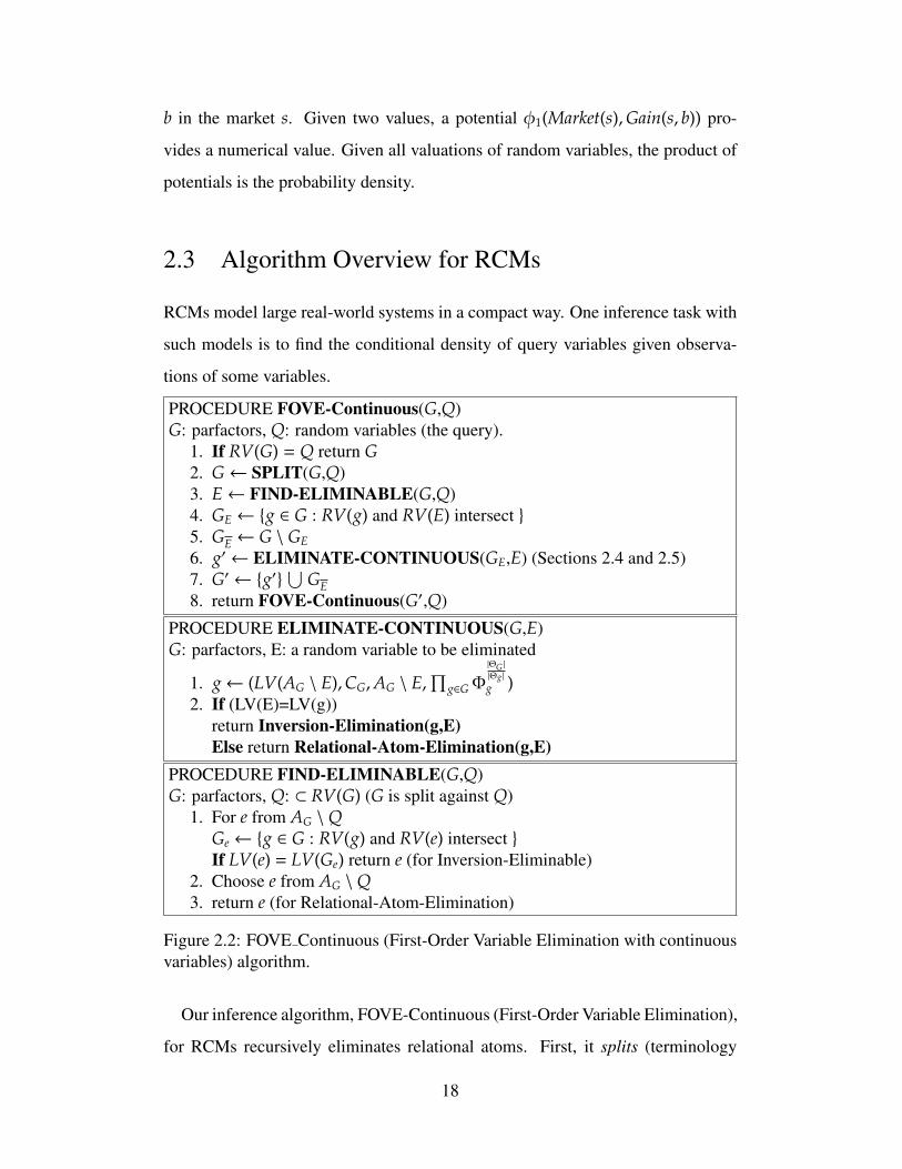
2.2 FOVE Continuous (First-Order Variable Elimination with con-tinuous variables) algorithm. . . . . . . . . . . . . . . . . . . . . 18

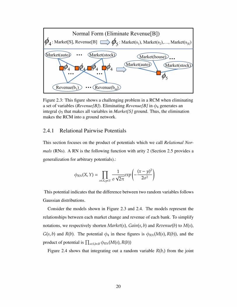
2.3 This figure shows a challenging problem in a RCM when elim-inating a set of variables (Revenue[B]). Eliminating Revenue[B]in φ4 generates an integral φ5 that makes all variables in Mar-ket[S] ground. Thus, the elimination makes the RCM into aground network. . . . . . . . . . . . . . . . . . . . . . . . . . . 20

2.4 This figure shows our method for the problem shown in Fig-ure 2.3. When eliminating Revenue[B], we do not generatea ground network. Instead, we directly generate the pairwiseform which allows the inference at the lifted level. . . . . . . . . . 21

2.5 Inference time with different number of banks . . . . . . . . . . . 312.6 Inference time with different number of markets . . . . . . . . . 32

3.1 Example of a housing market model. We are interested in esti-mating the hidden value of houses given observations of housesales prices (e.g. HPOt(1) = $500K). Both, the hidden valueof a house and the observed sales prices are affected by severalfactors, e.g., house values increase by a certain rate every yearand are also influenced by a housing market index (HMt). . . . . 39

xi

3.2 This model has three relational atoms, Xi, which may repre-sent any number of random variables. The relational represen-tation dramatically eliminates the need for redundant poten-tials. Hence, representation and filtering become much moreefficient than in the propositional case. Note that the conven-tional KF representation is not suited for efficient (i.e. lifted)inference. . . . . . . . . . . . . . . . . . . . . . . . . . . . . . . 40

3.3 Algorithm Lifted Relational Kalman Filter for Relational Gaus-sian Models. . . . . . . . . . . . . . . . . . . . . . . . . . . . . . 49

3.4 Average filtering time with increasing number of houses. Notethe cubic increase in filtering time for the Ground Kalman fil-ter and the linear increase for our Lifted Relational Kalmanfilter (LRKF). The y-axis is shown in logarithmic scale. Toshow that LRKF performs linearly, we added markers at themeasurements on the LRKF curve. . . . . . . . . . . . . . . . . 52

4.1 Graphical model on the domain of the election of one of twoparties A and B. The random variable Ads indicates whichparty has the most ads in the media. The variables Vi indi-cate the vote of each person in a population, modeled as a de-pendence of ad exposure. The Winner variable indicates thewinner and it is determined by the majority (MODE) of votes.One would like to estimate the probability of each party win-ning the election given this model. . . . . . . . . . . . . . . . . . 59

4.2 Histogram with a binomial distribution with (a) equality and(b) inequality constraints. . . . . . . . . . . . . . . . . . . . . . . 65

4.3 Histogram space for multinomial distributions with (a) equal-ity and (b) inequality constraints. . . . . . . . . . . . . . . . . . . 68

4.4 Ratios of utilities of approximate algorithms and exact method(histogram based counting). . . . . . . . . . . . . . . . . . . . . . 73

4.5 Error curves for different values of k and n. . . . . . . . . . . . . 74

5.1 An illustration of factoring a potential φXY(Xn,Ym). Our al-gorithm converts a RHM (left) into a variational (or factored)RHM (right) where the probability is represented by only twolatent variables LX and LY. . . . . . . . . . . . . . . . . . . . . . 79

5.2 Algorithm Lifted Relational Variational Inference (LRVI). . . . . 815.3 Algorithm Find-Variational-RHM (Section 5.5). . . . . . . . . . . 815.4 Algorithm Latent-Variable-Elimination (Section 5.6). . . . . . . . 82

xii

5.5 Illustrations of three different value-histograms of 10 exchange-able discrete rvs. Dotted lines with markers represent the bestpossible variational approximation, i.e., the binomial distri-bution for discrete rvs. (a) presents a potential, which is notextendible to n>10 because of the single bar at 8. (b) and(c) respectively present potentials extendible up to 20 and 100rvs. For a potential in (1), the variational approximation hasa high error, TVD, and thus is not appropriate. When a po-tential is extendible to a number larger than 10, the variationalapproximation is reasonably small as shown in (2) and (3). . . . . 90

5.6 The TVD of our variational models with k components. Whenk is a reasonable size (e.g. 32), the TVD is very small even fora large number of components (e.g. 1024) in the target distributions. 92

5.7 Locations of clustered wells A and B in the RRCA dataset. . . . . 955.8 Learned empirical distributions, Cdfs (FlA,u(x) and FlB,u′ (x)), of

rvs in groups A and B. . . . . . . . . . . . . . . . . . . . . . . . 955.9 A factored variational model for a continuous atom HPm, the

price change of each house, and a discrete atom Jobn, whethereach individual has a job. . . . . . . . . . . . . . . . . . . . . . . 96

5.10 Figure (a) compares the accuracy of our lifted MCMC and theground MCMC with various numbers of houses. ‘()’ indicatesthe number of houses (e.g. ‘Ground(16)‘ is the ground MCMCwith 16 houses, and ‘Lifted(16)‘ is the lifted MCMC with 16houses). Figure (b) shows the average sampling time per eachtime step with various number of houses. . . . . . . . . . . . . . . 97

xiii

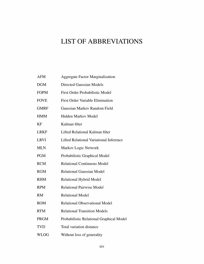
LIST OF ABBREVIATIONS

AFM Aggregate Factor Marginalization

DGM Directed Gaussian Models

FOPM First Order Probabilistic Model

FOVE First Order Variable Elimination

GMRF Gaussian Markov Random Field

HMM Hidden Markov Model

KF Kalman filter

LRKF Lifted Relational Kalman filter

LRVI Lifted Relational Variational Inference

MLN Markov Logic Network

PGM Probabilistic Graphical Model

RCM Relational Continuous Model

RGM Relational Gaussian Model

RHM Relational Hybrid Model

RPM Relational Pairwise Model

RM Relational Model

ROM Relational Observational Model

RTM Relational Transition Models

PRGM Probabilistic Relational Graphical Model

TVD Total variation distance

WLOG Without loss of generality

xiv

CHAPTER 1

INTRODUCTION

This thesis presents new insights and algorithms for Probabilistic Graphical Mod-

els (PGMs). A PGM is a graphical representation of a joint probability distribution

over random variables. Each node in the graph represents a random variable. Each

factor in the graph represents a joint probability over a subset of the random vari-

ables. By grouping random variables, Probabilistic Relational Graphical Models

(PRGMs), or Relational Models (RMs), enable scaling up the representation and

learning of PGMs. Inference, answering questions, with the relational models

enables many current and future applications, such as medical informatics, en-

vironmental engineering, financial forecasting, and robot localizations. Scaling

inference algorithms for large models is a key challenge to scaling up current ap-

plications and enabling future ones.

Inference, computing various probabilities of interest, with large PRGMs is

hard because large graphs tend to include large cliques, sets of fully intercon-

nected random variables. In general, the computational solution of an inference

problem with such a model becomes exponentially harder as the number of ran-

dom variables in the largest clique increases. Thus, many inference problems for

large relational models are intractable.

This thesis delivers fresh insights into and algorithms for large-scale probabilis-

tic graphical models, including clustered random variables. It presents new ideas

that maintain a compact structure when solving inference problems for relational

models with continuous random models. The insights expand to a key contribu-

tion, the Lifted Relational Kalman filter (LRKF), an efficient estimation algorithm

for large-scale linear dynamic systems which shows that the LRKF enables scal-

1

ing the exact Kalman filter from 1,000 to 1,000,000,000 variables.

Another key contribution of this thesis is that it proves that regularly used prob-

abilistic first-order languages, including Markov Logic Networks (MLNs) and

First-Order Probabilistic Models (FOPMs), can be reduced to compact probabilis-

tic graphical representations under reasonable conditions. Specifically, this thesis

shows that aggregate factors and the existential quantification in the languages

are accurately approximated by linear constraints in the Gaussian distribution. In

general cases, variational models approximate PRGMs with bounded errors. Vari-

ational models also pave the way for solving inference problems efficiently. These

advances have been directly applied in real-world groundwater models [Xu et al.,

2012]. The similar principles also have been applied to multiple domains in com-

puter vision [Choi et al., 2011c; 2008], robot planning [Choi and Amir, 2007;

2009], network abuse detection [Choi et al., 2010b] and decision making [Ha-

jishirzi et al., 2009].

1.1 Inference with Relational Hybrid Models

1.1.1 Overview

Relational Hybrid Models (RHMs) represent relationships among sets of random

variables with continuous and discrete domains in a concise manner. The intuition

of RHMs is that each set of random variables has the same numbers and types of

relationships as other sets. For example, prices of houses in the same residential

district may change together. Two random variables, representing the prices of a

house A and a neighboring house B, may have the same relationship with another

random variable, the mortgage rate. Thus, one may also model the relationship

with the same factor, e.g., having the same Gaussian noise.

In this thesis, probabilistic first-order language describes relationships among

sets of discrete and continuous random variables for the RHMs. The probabilis-

tic language handles uncertainty using probability theory and exploits structure

2

using first-order logic. The language provides an expressive formalism that repre-

sents the joint probability distribution of a large number of random variables. The

language first defines a first-order logic sentence over the universe of random vari-

ables. Any set of random variables satisfied by the first-order logic sentence has

the same factor over the set of random variables. In this way, the relational models

can compactly represent the joint probability distribution without redundancies.

The language allows the utilization of the first-order structure for efficient in-

ference. It is well known that first-order logic allows for efficient reasoning proce-

dures by enumerating first-order logic sentences without referring to all proposi-

tional, or individual, elements. Lifted inference algorithms can calculate the con-

ditional and marginal probabilities for RHMs by uplifting the model structures

and referring only to first-order relationships, not all propositional variables.

1.1.2 What Is the Problem?

Many real-world systems in finance, environmental engineering, and robotics in-

clude continuous domains. One cannot avoid dealing with continuous random

variables when answering questions about the systems. Unfortunately, most prin-

ciples devised for discrete RMs, e.g. [Poole, 2003; de Salvo Braz et al., 2005;

Milch and Russell, 2006; Richardson and Domingos, 2006], are not applicable to

such complex continuous systems and require discretizing continuous domains.

Furthermore, discretization and usage of discrete lifted inference algorithms is

highly imprecise. Therefore, the first fundamental challenge addressed in this

thesis is building probabilistic representation languages and efficient inference al-

gorithms for RMs with continuous variables.

Another key challenge is handling individual attributes of random variables in

relational models. For example, an RM can represent a housing market model in a

country. The models should be able to handle the price of each house in the coun-

try. However, most existing lifted inference algorithms force random variables to

have the exact same attributes so they are in the same group. Thus, whenever new

3

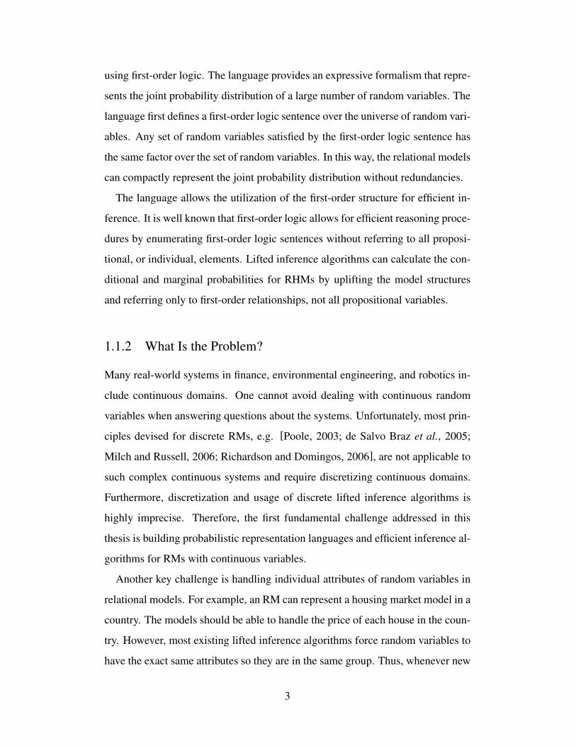
Relational Hybrid Models

Continuous Discrete

O(n3)

Gaussian

O(n3)

Observations

Exchangeable RVs

O(exp(m)) O(exp(n)) O(exp(n))

Aggregate Factors

𝐎(log 𝐧)

𝐎 𝐞𝐱𝐩 𝐦∗ 𝐎 𝐞𝐱𝐩 𝐦

∗

𝐎(𝐧) 𝐎(𝐧)

𝐎 𝐜 ∗ 𝐂𝐡𝐚𝐩𝐭𝐞𝐫 2

𝐂𝐡𝐚𝐩𝐭𝐞𝐫 3

𝐂𝐡𝐚𝐩𝐭𝐞𝐫 4

𝐂𝐡𝐚𝐩𝐭𝐞𝐫 5

Figure 1.1: An illustration of the contributions of this thesis. The complexitiesdisplayed with bold fonts represent the new results of this thesis on solvinginference problems with RHMs. Here, n is the number of random variables(RVs); m is the number of RV clusters; c is a constant; and ∗ represents anapproximation. Aggregate factors and exchangeable RVs will be defined in therelevant chapters.

attributes are given or observed in an individual random variable, the attributes

force the lifted inference algorithms to deteriorate the first-order structures into

fine-grained propositional structures. Given such propositional structures, lifted

inference algorithms refer to all ground random variables, and do as badly as

propositional inference algorithms.

1.1.3 The Contributions of This Thesis

This thesis introduces new lifted inference algorithms that compute the condi-

tional (or marginal) probability of RHMs. The first contribution (Chapter 2) is a

new lifted inference algorithm for RMs with only continuous variables, or Rela-

tional Continuous Models (RCMs). The algorithm maintains relational structures

during the inference procedure for relational pair-wise potentials, such as pairwise

linear Gaussian potentials.

The second contribution (Chapter 3) is an efficient exact filtering algorithm,

4

the LRKF, for large-scale linear dynamic systems. In each time step, the lifted

inference algorithm efficiently updates a large number of random variables. The

LRKF maintains compact pairwise relationships among random variables even

with individual observations. Thus, individual attributes do not degenerate the

relational structures into propositional ones.

The third contribution (Chapter 4) is a new insight into aggregate operations in

RMs1. It shows that aggregate operators over relational models can be accurately

approximated using linear constraints over Gaussian distributions. Thus, in many

cases, calculating the conditional probability does not depend on the number of

random variables. The accuracy of approximation is close to optimal when the

model has a large number of random variables.

The last contribution (Chapter 5) includes new variational models, which present

a new understanding of RHMs and variational models. One of the key under-

standings is that some potentials over sets of random variables in RHMs can be

represented by a mixture of a joint probability distribution over independent and

identically distributed (i.i.d.) random variables. The variational models seam-

lessly represent the discrete and continuous variables in the unified framework.

1.2 The Technical Results of This Thesis

1.2.1 Efficient Inference with Relational Continuous Models

Calculating a marginal over variables of interest is a typical inference task. At

a propositional level, inference with a large number of continuous variables is

non-trivial. Suppose that a random variable representing the market index such

as S&P 500 depends directly on n random variables, revenues of n banks. When

marginalizing the market index variable out, the marginal is a function of n vari-

ables (revenues of banks), thus marginalizing out remaining variables becomes

1Aggregate operators in RMs are equivalent to the existential quantification the probabilisticfirst-order languages

5

harder. When n grows, the computation becomes expensive. For example, when

relations among variables follow Gaussian distributions, the computational com-

plexity of the inference problem is O(|U|3) (U is a set of random variables). It

limits the uses of such relational models to many large-scale real-world applica-

tions.

To address these issues, Probabilistic Relational Models (PRMs) [Ng and Sub-

rahmanian, 1992; Koller and Pfeffer, 1997; Pfeffer et al., 1999; Friedman et al.,

1999; Poole, 2003; de Salvo Braz et al., 2005; Richardson and Domingos, 2006;

Milch and Russell, 2006; Getoor and Taskar, 2007] describe probability distribu-

tions at a relational level with the purpose of capturing larger models. PRMs

combine probability theory for handling uncertainty and relational models for

representing system structures compactly. Thus, they facilitate construction and

learning of probabilistic models for large systems. Recently, [Poole, 2003; de

Salvo Braz et al., 2005; Milch et al., 2008; Singla and Domingos, 2008] showed

that such models enable more efficient inference than possible with propositional

graphical models, when inference occurs directly at the relational level.

Present exact lifted inference algorithms [Poole, 2003; de Salvo Braz et al.,

2006; Milch et al., 2008] and those developed in the efforts above are suitable for

discrete domains, thus can in theory be applied to continuous domains through

discretization. However, the precision of discretizations deteriorates exponen-

tially in the number of dimensions in the model, and the number of dimensions in

relational models is the number of ground random variables. Thus, discretization

and usage of discrete lifted inference algorithms is highly imprecise.

Here, this thesis presents the first exact lifted inference algorithm for Relational

Continuous Models (RCMs), a new probabilistic first-order language for contin-

uous domains. The main insight is that, for some classes of potential functions

(or potentials), marginalizing out a ground random variable in a RCM can yield a

RCM representation that does not force other random variables to become propo-

sitional. Further, relational pairwise models, i.e. products of relational potentials

of arity 2, remain relational pairwise models after eliminating out ground random

6

variables in those models. Thus, it leads to the compact representations and the

efficient computations. I report Gaussian potentials, which satisfy the conditions

for relational pairwise models.

This thesis also adapts principles of Inversion Elimination, a method devised

by [Poole, 2003], to continuous models. Inversion Elimination’s step essentially

takes advantage of an ability to exchange sums and products. The lifted exchange

of sums and products translates directly to continuous domains. This is a unique

approach to continuous models.

Given a RCM, the suggested algorithm marginalizes continuous variables by

analytically integrating out random variables except query variables. It does so by

finding a variable, and eliminating it by Inversion Elimination. If such elimination

is not possible, Relational Atom Elimination eliminates each pairwise form in a

linear time. If the marginal is not in pairwise form, it converts the marginal into a

pairwise form.

1.2.2 The Lifted Relational Kalman Filtering

The Kalman filter (KF) [Kalman, 1960] accurately estimates the state of a dy-

namic system given a sequence of control-inputs and observations. It has been

applied in a broad range of domains which include weather forecasting [Burgers et

al., 1998], localization and tracking in robotics [Limketkai et al., 2005], economic

forecasting [Bahmani-Oskooee and Brown, 2004] and many others. Given a se-

quence of observations and Gaussian dependences between variables, the filtering

problem is to calculate the conditional probability density of the state variables

at each timestep. Unfortunately, the KF computations are cubic in the number

of random variables, which limits the use of the KF exact methods to domains

with a limited number of random variables. This has led to the combination of

approximation and sampling (e.g. the Ensemble Kalman filter [Evensen, 1994]).

The LRKF leverages the power of relational languages [Friedman et al., 1999;

Poole, 2003; Richardson and Domingos, 2006] to describe models of which rep-

7

resentations are independent of the size of populations involved. Various lifted

inference algorithms for relational models have been proposed [Poole, 2003; de

Salvo Braz et al., 2005; Milch and Russell, 2006; Richardson and Domingos,

2006; Wang and Domingos, 2008; Choi et al., 2010a]. These seek to achieve

carry computations in time independent of the size of the populations involved.

However, the key challenge in relational filtering (of dynamic systems) is ensur-

ing that the representation does not deteriorate to the ground case when multiple

observations are made. As more observations are received, an increasing num-

ber of objects become distinguished. This precludes the use of previously known

algorithms unless approximately equivalent objects are grouped with expensive

clustering algorithms.

This thesis presents Relational Gaussian Models (RGMs) to model dynamic

systems of a large number of variables in a relational fashion. RGMs have as their

main building block the pairwise linear Gaussian potential as detailed in Section

3.2. Further, it proposes a new lifted filtering algorithm that marginalizes out

random variables of the previous timestep efficiently, in time linear in the number

of random variables, while maintaining the relational (RGM) representation.

This prevents the relational pairwise structure from being increasingly grounded

even when individual observations are made for all random variables. Moreover,

updating the relational model takes only quadratic in the number of relational

atoms (sets of random variables).

One key insight is that, given identical observation models, even when the

means of the random variables are dispersed their variances remain identical. This

is sufficient to sustain a relational representation.

1.2.3 Efficient Inference with Aggregate Factors in RelationalModels

Relational models can compactly (that is, intensionally) represent graphical mod-

els involving a large number of random variables, each of them representing a rela-

8

tion between objects in a domain [Koller and Pfeffer, 1997; Friedman et al., 1999;

Milch et al., 2005; Richardson and Domingos, 2006].

While it is possible to take advantage of compactness only for representation

and expand the model into a propositional (extensional) form for inference, lifted

inference methods try to keep the representation as compact as possible even

during inference, increasing efficiency [Poole, 2003; de Salvo Braz et al., 2007;

Milch et al., 2008; Singla and Domingos, 2008] .

The first proposed lifted inference solutions could deal only with factors on a

fixed number of random variables. Aggregate parametric factors (based on aggre-

gate functions such as OR, MAX, AND, SUM, AVERAGE, MODE and MEDIAN),

which are defined on a varying, intensionally defined set of random variables, still

needed to be treated propositionally, with cost exponential in the number n of

random variables.

[Kisynski and Poole, 2009] introduced lifted methods for aggregate factors that

reduce this complexity to O(rk log n) for commutative associative aggregate func-

tions on n k-valued random variables being aggregated into an r-valued random

variable (and even O(rk) for OR and MAX)2. However, for general cases (such

as the non-associative function MODE), their exact inference process has time

O(rnk), that is, polynomial in n.

Here, the contributions of this chapter are threefold. It contributes an exact

solution constant in n when k = 2 for aggregate operations AND, OR, MAX and

SUM.

It also presents an efficient (constant in n) approximate algorithm for inference

with aggregate factors, for all typical aggregate functions.

The potential of an aggregate factor for a valuation v of a set of random vari-

ables depends only on the histogram on the distribution of k values in V (in what

[Milch et al., 2008] calls a counting formula).

This chapter shows that the typical aggregate functions but for XOR3 can be

2Note that r=n for aggregate functions such as SUM of n binary variables.3XOR has its own straightforward solution.

9

represented by linear constraints in the space of histograms (a (k−1)-simplex).

Because aggregate factors’ potentials on the space of histograms can be approx-

imated by a normal distribution, one can approximately sums over them (which

is the main inference operation) by computing the volume under normal distribu-

tions truncated by linear constraints. This holds even for MODE, which is com-

mutative but not associative.

This approximation can be computed analytically for all operations on binary

random variables and for certain operations on multivalued (k>2) random vari-

ables such as SUM and MEDIAN. Otherwise, it is computed by Gibbs sampling

with a limited number of iterations [Geweke, 1991; Damien and Walker, 2001].

Finally, a third contribution is a further optimization for aggregations of multiple

groups of random variables, each with its own distribution.

1.2.4 Lifted Relational Variational Models

Many real-world systems can be described using continuous and discrete variables

with relations among them. Such examples include measurements in environmen-

tal sensor networks, localizations in robotics, and economic forecasting in finance.

In such large systems, efficient and precise inference is necessary. As an example

from environmental science, an inference algorithm can predict a posterior of un-

observed groundwater levels and contamination levels at different locations, and

making such an inference precisely is critical to decision makers.

Probabilistic Relational Models (PRMs) [Ng and Subrahmanian, 1992; Pfeffer

et al., 1999; Friedman et al., 1999; Richardson and Domingos, 2006] describe

probability distributions at a relational level with the purpose of capturing the

structure of larger models. These compact representations can facilitate the con-

struction and learning of probabilistic models for large systems. A key challenge

of inference procedures with RPLs is that they often result in intermediate den-

sity functions involving many random variables and complex relationship among

them.

10

Real-world systems have large numbers of variables including both discrete

and continuous. PRMs represent such large systems compactly. Lifted inference

presently can address discrete models and continuous models, but not hybrid ones.

For (d-valued) discrete variables, lifted inference can take advantage of the insight

which groups equivalent models into a histogram representation with an order

of poly(d) entries [de Salvo Braz et al., 2005; Milch and Russell, 2006; Jha et

al., 2010] (instead of exp(d) entries in traditional ground models). For Gaussian

potentials, lifted inference algorithms can maintain a compact covariance matrix

during (and after) inference, e.g. [Choi et al., 2010a; 2011b].

Unfortunately, these principles are not applicable to general (non-Gaussian)

hybrid models because the histogram is not applicable to continuous domains

without discretizations, and the covariance matrix is a special structure for Gaus-

sians. Thus, existing variational methods, e.g. Latent Tree Models [Zhang, 2002;

Choi et al., 2011d] and Nonparametric Bayesian Logic [Carbonetto et al., 2005],

focus either on discrete models or Gaussian models.

This thesis provides a new insight (relational variational-inference lemmas)

which accurately factors densities of relational models into mixtures of i.i.d. ran-

dom variables. These lemmas enable us to build a variational approximation al-

gorithm that takes large-scale graphical models with hybrid variables and finds

close-to-optimal relational variational models. Then, lifted inference algorithms, a

variable elimination and a Markov chain Monte Carlo (MCMC) sampling method,

efficiently solve marginal inference problems on the variational models. This the-

sis shows that the algorithm gives a better solution than previous ones.

1.3 Plan of This Thesis

The main contributions of the thesis are included in Chapters 2, 3, 4 and 5. Chapter

2 formally defines RCMs, which are relational models with pairwise continuous

potentials. Then, it presents an efficient inference algorithm for pairwise Gaussian

11

potentials. Chapter 3 extends the algorithm of Chapter 2 to create the LRKF,

a new relational Kalman filter for relational linear dynamic systems. Chapter 4

presents lifted inference algorithms with aggregate factors. Chapter 5 presents a

unified framework for relational hybrid models with the perspective of variational

models. Chapter 6 summarizes the thesis and suggests opportunities for future

studies.

Each chapter is written in an independent manner without assuming that readers

have any background knowledge in relational models. Thus, it should be compre-

hensible to readers in computer science and other fields of science and engineer-

ing. Readers who are interested in Kalman Filtering should refer to Chapter 3.

Those who are interested in variational inference should refer to Chapter 5.

1.4 Publication Notes

Below is the list of publications and chapters where they are revised and used :

• [Choi et al., 2010a]: Chapter 2

• [Choi et al., 2011b]: Chapter 3

• [Choi et al., 2011a]: Chapter 4

• [Choi and Amir, 2011; 2012]: Chapter 5

12

CHAPTER 2

LIFTED INFERENCE FOR RELATIONALCONTINUOUS MODELS

Relational Continuous Models (RCMs) represent joint probability densities over

attributes of objects, when the attributes have continuous domains. With rela-

tional representations, they can model joint probability distributions over large

numbers of variables compactly in a natural way. This section presents a new ex-

act lifted inference algorithm for RCMs, thus it scales up to large models of real

world applications. The algorithm applies to Relational Pairwise Models which

are (relational) products of potentials of arity 2. Our algorithm is unique in two

ways. First, it substantially improves the efficiency of lifted inference with vari-

ables of continuous domains. When a relational model has Gaussian potentials,

it takes only linear-time compared to cubic time of previous methods. Second, it

is the first exact inference algorithm which handles RCMs in a lifted way. The

algorithm is illustrated over an example from econometrics. Experimental results

show that our algorithm outperforms both a ground-level inference algorithm and

an algorithm built with previously-known lifted methods.

2.1 Introduction

Many real world systems are described by continuous variables and relations

among them. Such systems include measurements in environmental-sensors net-

works [Hill et al., 2009], localizations in robotics [Limketkai et al., 2005], and

economic forecastings in finance [Niemira and Saaty, 2004]. Once a relational

model among variables is given, inference algorithms can solve value prediction

problems and classification problems.

13

At a ground level, inference with a large number of continuous variables is non-

trivial. Typically, inference is the task of calculating a marginal over variables of

interest. Suppose that a market index has a relationship with n variables, revenues

of n banks. When marginalizing out the market index, the marginal is a function

of n variables (revenues of banks), thus marginalizing out remaining variables be-

comes harder. When n grows, the computation becomes expensive. For example,

when relations among variables follow Gaussian distributions, the computational

complexity of the inference problem is O(|U|3) (U is a set of ground variables).

Thus, the computation with such models is limited to moderate-size models, pre-

venting its use in the many large, real-world applications.

To address these issues, Probabilistic Relational Models (PRMs) [Ng and Sub-

rahmanian, 1992; Koller and Pfeffer, 1997; Pfeffer et al., 1999; Friedman et al.,

1999; Poole, 2003; de Salvo Braz et al., 2005; Milch et al., 2005; Richardson and

Domingos, 2006; Milch and Russell, 2006; Getoor and Taskar, 2007] describe

probability distributions at a relational level with the purpose of capturing larger

models. PRMs combine probability theory for handling uncertainty and rela-

tional models for representing system structures. Thus, they facilitate construction

and learning of probabilistic models for large systems. Recently, [Poole, 2003;

de Salvo Braz et al., 2005; Milch et al., 2008; Singla and Domingos, 2008]

showed that such models enable more efficient inference than possible with propo-

sitional graphical models, when inference occurs directly at the relational level.

Present exact lifted inference algorithms [Poole, 2003; de Salvo Braz et al.,

2006; Milch et al., 2008] and those developed in the efforts above are suitable for

discrete domains, thus can in theory be applied to continuous domains through

discretization. However, the precision of discretizations deteriorates exponen-

tially in the number of dimensions in the model, and the number of dimensions in

relational models is the number of ground random variables. Thus, discretization

and usage of discrete lifted inference algorithms is highly imprecise.

Here, we propose the first exact lifted inference algorithm for Relational Con-

tinuous Models (RCMs), a new relational probabilistic language for continuous

14

domains. Our main insight is that, for some classes of potential functions (or po-

tentials), marginalizing out a ground random variable in a RCM can yield a RCM

representation that does not force other random variables to become propositional

(Section 2.4). Further, relational pairwise models, i.e. products of relational po-

tentials of arity 2, remain relational pairwise models after eliminating out ground

random variables in those models. Thus, it leads to the compact representations

and the efficient computations. We report Gaussian potentials which satisfy the

conditions for relational pairwise models (Section 2.5). However, we are unsure

whether the conditions are only satisfied by Gaussian potentials, yet.

We also adapt principles of Inversion Elimination, a method devised by [Poole,

2003], to continuous models. Inversion Elimination’s step essentially takes ad-

vantage of an ability to exchange sums and products. The lifted exchange of sums

and products translates directly to continuous domains. This is a unique approach

to continuous models, even though the insight is brought from discrete models.

Given a RCM, our algorithm marginalizes continuous variables by analytically

integrating out random variables except query variables. It does so by finding a

variable, and eliminating it by Inversion Elimination. If such elimination is not

possible, Relational Atom Elimination eliminates each pairwise form in a linear

time. If the marginal is not in pairwise form, it converts the marginal into a pair-

wise form.

This chapter is organized as follows. Section 2.2 provides the formal definition

of RCMs. Section 2.3 overviews our inference algorithms. Section 2.4 presents

main intuitions and results in a Gaussian potential. Section 2.5 provides the gener-

alized algorithm for relational pairwise models. Section 2.7 provides experimental

results followed by related works in Section 2.6. It concludes in Section 2.8.

15

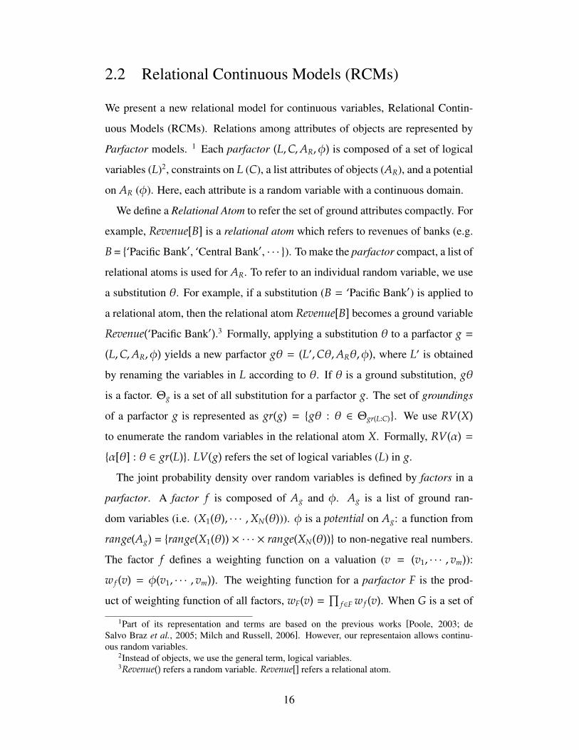
2.2 Relational Continuous Models (RCMs)

We present a new relational model for continuous variables, Relational Contin-

uous Models (RCMs). Relations among attributes of objects are represented by

Parfactor models. 1 Each parfactor (L,C,AR, φ) is composed of a set of logical

variables (L)2, constraints on L (C), a list attributes of objects (AR), and a potential

on AR (φ). Here, each attribute is a random variable with a continuous domain.

We define a Relational Atom to refer the set of ground attributes compactly. For

example, Revenue[B] is a relational atom which refers to revenues of banks (e.g.

B = {‘Pacific Bank′, ‘Central Bank′, · · · }). To make the parfactor compact, a list of

relational atoms is used for AR. To refer to an individual random variable, we use

a substitution θ. For example, if a substitution (B = ‘Pacific Bank′) is applied to

a relational atom, then the relational atom Revenue[B] becomes a ground variable

Revenue(‘Pacific Bank′).3 Formally, applying a substitution θ to a parfactor g =

(L,C,AR, φ) yields a new parfactor gθ = (L′,Cθ,ARθ, φ), where L′ is obtained

by renaming the variables in L according to θ. If θ is a ground substitution, gθ

is a factor. Θg is a set of all substitution for a parfactor g. The set of groundings

of a parfactor g is represented as gr(g) = {gθ : θ ∈ Θgr(L:C)}. We use RV(X)

to enumerate the random variables in the relational atom X. Formally, RV(α) =

{α[θ] : θ ∈ gr(L)}. LV(g) refers the set of logical variables (L) in g.

The joint probability density over random variables is defined by factors in a

parfactor. A factor f is composed of Ag and φ. Ag is a list of ground ran-

dom variables (i.e. (X1(θ), · · · ,XN(θ))). φ is a potential on Ag: a function from

range(Ag) = {range(X1(θ)) × · · · × range(XN(θ))} to non-negative real numbers.

The factor f defines a weighting function on a valuation (v = (v1, · · · , vm)):

w f (v) = φ(v1, · · · , vm)). The weighting function for a parfactor F is the prod-

uct of weighting function of all factors, wF(v) =∏

f∈F w f (v). When G is a set of

1Part of its representation and terms are based on the previous works [Poole, 2003; deSalvo Braz et al., 2005; Milch and Russell, 2006]. However, our representaion allows continu-ous random variables.

2Instead of objects, we use the general term, logical variables.3Revenue() refers a random variable. Revenue[] refers a relational atom.

16

Loss(s,b): Loss of a bank(b) in a market(s) (e.g. -$0.2B)Market(s): Market index of a sector(s) (e.g.-5.3%)

Revenue(b): Revenue of a bank(b) (eg. +$0.3B)

Recession: Recession index of a country (e.g. -4.3%)

Market(auto) Market(stock)

Loss(auto,b1) Loss(stock,b1) Loss(stock,bm)Loss(auto,bm)

Revenue(b1) Revenue(bm)

… … …

…

…

potential functioneg. -5.3%

φ 2φ 2φ 2 φ 2

φ 3 φ 3φ 3φ 3

eg. -$0.2B

eg. +$0.3B

Recession

φ1 φ 1

eg. -4.3%

bank1

S = {auto, house, …, stock} B = {b1, b2, …, bm}Market[S] = {Market(auto), Market(house), …, Market(stock)}

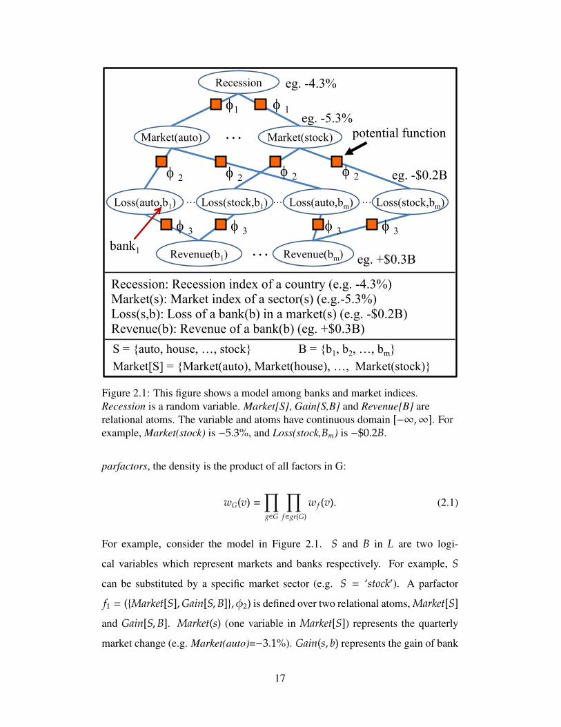
Figure 2.1: This figure shows a model among banks and market indices.Recession is a random variable. Market[S], Gain[S,B] and Revenue[B] arerelational atoms. The variable and atoms have continuous domain [−∞,∞]. Forexample, Market(stock) is −5.3%, and Loss(stock,Bm) is −$0.2B.

parfactors, the density is the product of all factors in G:

wG(v) =∏g∈G

∏f∈gr(G)

w f (v). (2.1)

For example, consider the model in Figure 2.1. S and B in L are two logi-

cal variables which represent markets and banks respectively. For example, S

can be substituted by a specific market sector (e.g. S = ‘stock′). A parfactor

f1 = ({Market[S],Gain[S,B]}, φ2) is defined over two relational atoms, Market[S]

and Gain[S,B]. Market(s) (one variable in Market[S]) represents the quarterly

market change (e.g. Market(auto)=−3.1%). Gain(s, b) represents the gain of bank

17

b in the market s. Given two values, a potential φ1(Market(s),Gain(s, b)) pro-

vides a numerical value. Given all valuations of random variables, the product of

potentials is the probability density.

2.3 Algorithm Overview for RCMs

RCMs model large real-world systems in a compact way. One inference task with

such models is to find the conditional density of query variables given observa-

tions of some variables.

PROCEDURE FOVE-Continuous(G,Q)G: parfactors, Q: random variables (the query).

1. If RV(G) = Q return G2. G← SPLIT(G,Q)3. E← FIND-ELIMINABLE(G,Q)4. GE← {g ∈ G : RV(g) and RV(E) intersect }5. GE← G \ GE

6. g′← ELIMINATE-CONTINUOUS(GE,E) (Sections 2.4 and 2.5)7. G′← {g′}

⋃GE

8. return FOVE-Continuous(G′,Q)

PROCEDURE ELIMINATE-CONTINUOUS(G,E)G: parfactors, E: a random variable to be eliminated

1. g← (LV(AG \ E),CG,AG \ E,∏

g∈G Φ|ΘG ||Θg |g )

2. If (LV(E)=LV(g))return Inversion-Elimination(g,E)Else return Relational-Atom-Elimination(g,E)

PROCEDURE FIND-ELIMINABLE(G,Q)G: parfactors, Q: ⊂ RV(G) (G is split against Q)

1. For e from AG \QGe← {g ∈ G : RV(g) and RV(e) intersect }If LV(e) = LV(Ge) return e (for Inversion-Eliminable)

2. Choose e from AG \Q3. return e (for Relational-Atom-Elimination)

Figure 2.2: FOVE Continuous (First-Order Variable Elimination with continuousvariables) algorithm.

Our inference algorithm, FOVE-Continuous (First-Order Variable Elimination),

for RCMs recursively eliminates relational atoms. First, it splits (terminology

18

of [Poole, 2003]; shattering in [de Salvo Braz et al., 2005])4 relational atoms.

The split operation makes groundings (e.g. RV(X) RV(Y)) of every relational

atoms (e.g. X Y) disjoint. It introduces observations as observations of ground-

ings of separate relational variables. For example, observing Market(auto) =

30% creates two separate relational atoms: Market(auto), Market(M)M,auto. The

‘M , auto’ then appears in parfactors relating to the latter relational atom. Af-

ter split, FIND-ELIMINABLE finds a relational atom which satisfies conditions

for one of the elimination algorithms: Inversion-Elimination (Section 2.5.2) and

Relational-Atom-Elimination (Section 2.5.3). The found atom is eliminated by

our ELIMINATE-CONTINUOUS algorithm explained in Sections 2.4 and 2.5. It

iterates the elimination until only query variables are remained. The procedure is

described in Figure 2.2.

Our main contributions are focused on the algorithm ELIMINATE-CONTIN-

UOUS, a lifted variable eliminations for continuous variables. We describe details

in Sections 2.4 and 2.5.

2.4 Inference with Gaussian Potentials

This section presents our first main technical contribution, efficient variable elim-

ination algorithms for relational Gaussian models. We focus on the inference

problem of computing the posterior of query variables given observations. It

is important to efficiently integrating out relational atoms (e.g. Revenue[B] =

{Revenue(b1), · · · , Revenue(bm)}) for solving this inference problem.

In the following description, we omit the (inequality between logical variables

and objects) constraints from parfactors. This allows us to focus on the potential

functions inside those parfactors. The treatment below holds with little change for

parfactors with such constraints.

4Please refer [Poole, 2003; de Salvo Braz et al., 2005] for further details.

19

5φ : Market(s1), Market(s2),…, Market(s|S|)

Normal Form (Eliminate Revenue[B])

4φ : Market[S], Revenue[B]

Market(auto) Market(stock)

Revenue(b1) Revenue(bm)

…

…

…

…Market(auto) Market(stock)

…Market(house)

5φ4φ4φ 4φ4φ

Figure 2.3: This figure shows a challenging problem in a RCM when eliminatinga set of variables (Revenue[B]). Eliminating Revenue[B] in φ4 generates anintegral φ5 that makes all variables in Market[S] ground. Thus, the eliminationmakes the RCM into a ground network.

2.4.1 Relational Pairwise Potentials

This section focuses on the product of potentials which we call Relational Nor-

mals (RNs). A RN is the following function with arity 2 (Section 2.5 provides a

generalization for arbitrary potentials).:

φRN(X,Y) =∏

x∈X,y∈Y

1

σ√

2πexp

(−

(x − y)2

2σ2

)

This potential indicates that the difference between two random variables follows

Gaussian distributions.

Consider the models shown in Figure 2.3 and 2.4. The models represent the

relationships between each market change and revenue of each bank. To simplify

notations, we respectively shorten Market(s), Gain(s, b) and Revenue(b) to M(s),

G(s, b) and R(b). The potential φ4 in these figures is φRN(M(s),R(b)), and the

product of potential is∏

s∈S,b∈B φRN(M(s),R(b))

Figure 2.4 shows that integrating out a random variable R(bi) from the joint

20

4φ : Market[S], Revenue[B] 5φ′: Market(si),Market(sj) (si,sj∈S)Pair-wise Form (Eliminate Revenue[B])

Market(auto) Market(stock)

Revenue(b1) Revenue(bm)

…

…

…

…Market(auto) Market(stock)

…Market(house)

∏∈

′Sss

jiji

ss,

5 ),(φ

5φ′5φ′

5φ′4φ4φ 4φ4φ

Figure 2.4: This figure shows our method for the problem shown in Figure 2.3.When eliminating Revenue[B], we do not generate a ground network. Instead, wedirectly generate the pairwise form which allows the inference at the lifted level.

density results in the product of RNs again (c and c’ are constants) as follow.

ˆR(bi)

∏s∈S

φ4(M(s),R(bi)) = c · exp(

(∑

s∈S M(s))2

2σ2 · |S|−

∑s∈S M(s)2

2σ2

)= c ·

∏1≤i< j≤|S|

exp(−

(M(si) −M(s j))2

2σ2 · |S|

)= c′ ·

∏1≤i< j≤|S|

φ′5(M(si),M(s j)) (2.2)

Note that, following equations holds for integration.

ˆR(bi)

exp(−aR(bi)

2 + 2bR(bi) + c)

=

√πa

exp(

b2

a+ c

)(2.3)

Here, the terms a and b can include random variables except R(bi).

Definition 1 (Connected Relational Normal) The product of RNs is connected,

when the connectivity graph is a connected component. Each vertex of the con-

nectivity graph is a random variable or a constant in RNs, and each edge is a

potential (RN). �

Lemma 1 The product of RNs is a probability density function when it is con-

nected, and at least a RN includes a constant argument.

The proof is provided in Section 2.9.

21

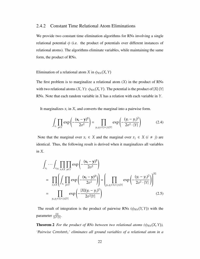
2.4.2 Constant Time Relational Atom Eliminations

We provide two constant time elimination algorithms for RNs involving a single

relational potential φ (i.e. the product of potentials over different instances of

relational atoms). The algorithms eliminate variables, while maintaining the same

form, the product of RNs.

Elimination of a relational atom X in φRN(X,Y)

The first problem is to marginalize a relational atom (X) in the product of RNs

with two relational atoms (X, Y): φRN(X,Y). The potential is the product of |X|·|Y|

RNs. Note that each random variable in X has a relation with each variable in Y.

It marginalizes xi in X, and converts the marginal into a pairwise form.

ˆxi

∏y∈Y

exp(−

(xi − y)2

2σ2

)=

∏yi,y j∈Y,i< j≤|Y|

exp(−

(yi − y j)2

2σ2 · |Y|

)(2.4)

Note that the marginal over xi ∈ X and the marginal over x j ∈ X (i , j) are

identical. Thus, the following result is derived when it marginalizes all variables

in X.

ˆx1

· · ·

ˆx|X|

∏xi∈X

∏y∈Y

exp(−

(xi − y)2

2σ2

)

=∏xi∈X

ˆxi

∏y∈Y

exp(−

(xi − y)2

2σ2

) =

∏yi,y j∈Y,i< j≤|Y|

exp(−

(yi − y j)2

2σ2 · |Y|

)|X|

=∏

yi,y j∈Y,i< j≤|Y|

exp(−|X|(yi − y j)2

2σ2|Y|

)(2.5)

The result of integration is the product of pairwise RNs (φRN(Y,Y)) with the

parameter |X|2σ2·|Y| .

Theorem 2 For the product of RNs between two relational atoms (φRN(X,Y)),

‘Pairwise Constant1’ eliminates all ground variables of a relational atom in a

22

constant time.

Proof Eliminating a variables xi in X takes a constant time shown as Equation

2.4. Eliminating other variables in X takes a constant time shown as Equation 2.5.

Thus, the computation takes only a constant time without an iteration. �

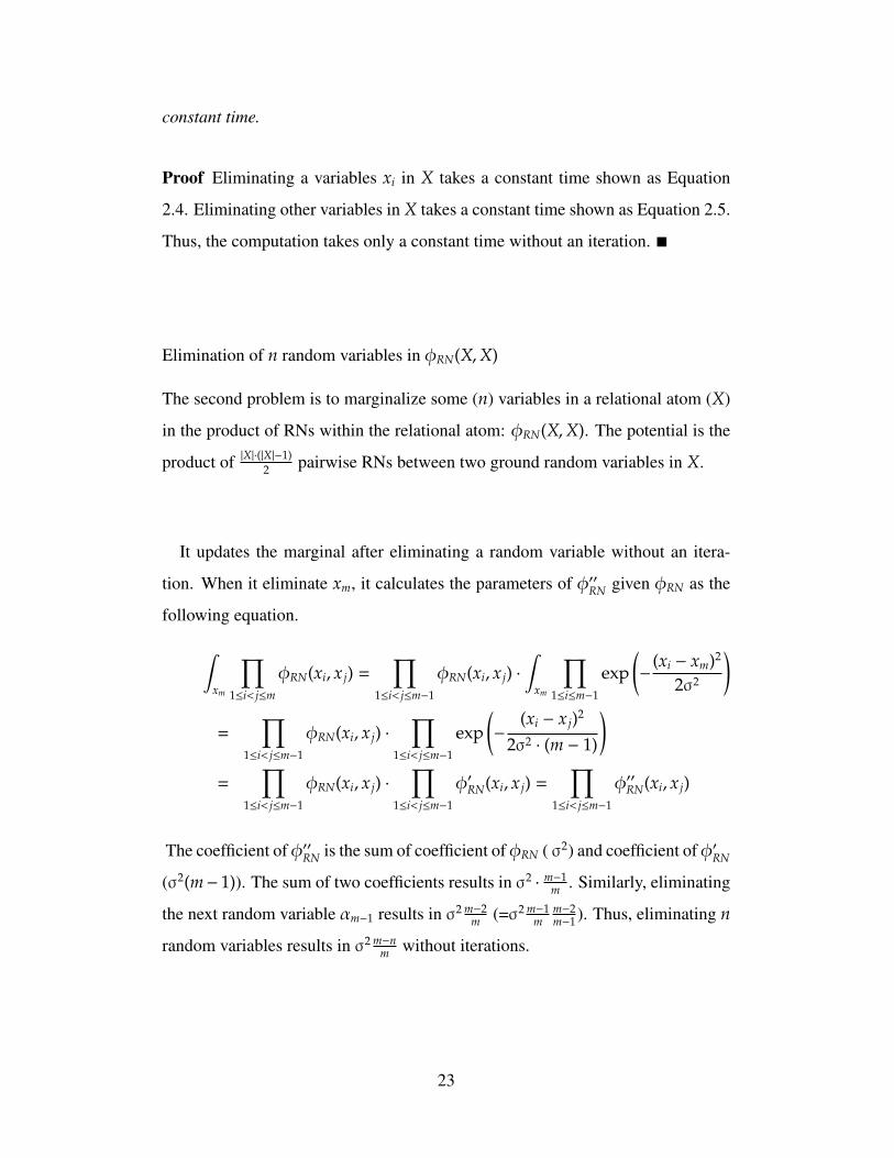
Elimination of n random variables in φRN(X,X)

The second problem is to marginalize some (n) variables in a relational atom (X)

in the product of RNs within the relational atom: φRN(X,X). The potential is the

product of |X|·(|X|−1)2 pairwise RNs between two ground random variables in X.

It updates the marginal after eliminating a random variable without an itera-

tion. When it eliminate xm, it calculates the parameters of φ′′RN given φRN as the

following equation.

ˆxm

∏1≤i< j≤m

φRN(xi, x j) =∏

1≤i< j≤m−1

φRN(xi, x j) ·ˆ

xm

∏1≤i≤m−1

exp(−

(xi − xm)2

2σ2

)

=∏

1≤i< j≤m−1

φRN(xi, x j) ·∏

1≤i< j≤m−1

exp(−

(xi − x j)2

2σ2 · (m − 1)

)=

∏1≤i< j≤m−1

φRN(xi, x j) ·∏

1≤i< j≤m−1

φ′RN(xi, x j) =∏

1≤i< j≤m−1

φ′′RN(xi, x j)

The coefficient ofφ′′RN is the sum of coefficient ofφRN ( σ2) and coefficient ofφ′RN

(σ2(m− 1)). The sum of two coefficients results in σ2·

m−1m . Similarly, eliminating

the next random variable αm−1 results in σ2 m−2m (=σ2 m−1

mm−2m−1 ). Thus, eliminating n

random variables results in σ2 m−nm without iterations.

23

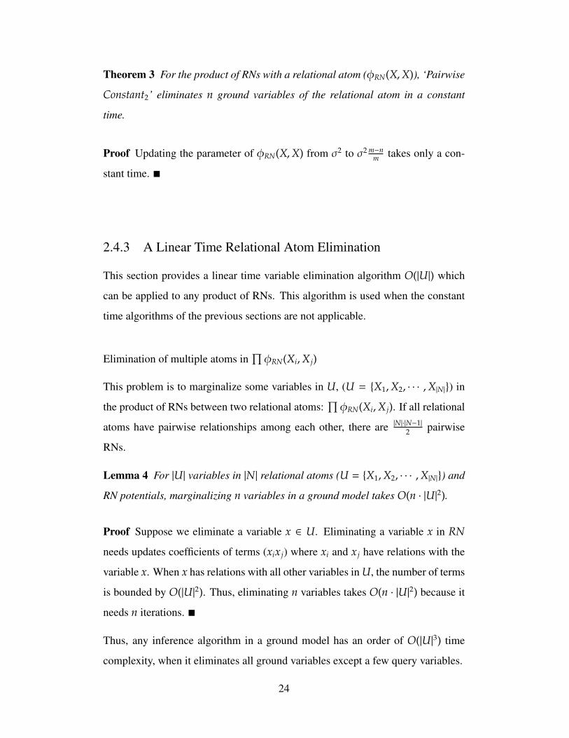
Theorem 3 For the product of RNs with a relational atom (φRN(X,X)), ‘Pairwise

Constant2’ eliminates n ground variables of the relational atom in a constant

time.

Proof Updating the parameter of φRN(X,X) from σ2 to σ2 m−nm takes only a con-

stant time. �

2.4.3 A Linear Time Relational Atom Elimination

This section provides a linear time variable elimination algorithm O(|U|) which

can be applied to any product of RNs. This algorithm is used when the constant

time algorithms of the previous sections are not applicable.

Elimination of multiple atoms in∏φRN(Xi,X j)

This problem is to marginalize some variables in U, (U = {X1,X2, · · · ,X|N|}) in

the product of RNs between two relational atoms:∏φRN(Xi,X j). If all relational

atoms have pairwise relationships among each other, there are |N|·|N−1|2 pairwise

RNs.

Lemma 4 For |U| variables in |N| relational atoms (U = {X1,X2, · · · ,X|N|}) and

RN potentials, marginalizing n variables in a ground model takes O(n · |U|2).

Proof Suppose we eliminate a variable x ∈ U. Eliminating a variable x in RN

needs updates coefficients of terms (xix j) where xi and x j have relations with the

variable x. When x has relations with all other variables in U, the number of terms

is bounded by O(|U|2). Thus, eliminating n variables takes O(n · |U|2) because it

needs n iterations. �

Thus, any inference algorithm in a ground model has an order of O(|U|3) time

complexity, when it eliminates all ground variables except a few query variables.

24

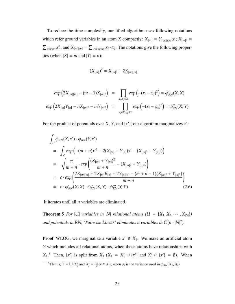
To reduce the time complexity, our lifted algorithm uses following notations

which refer ground variables in an atom X compactly: X[m] =∑

1≤i≤m xi; X[m]2 =∑1≤i≤m x2

i ; and X[m][m] =∑

1≤i< j≤m xi · x j. The notations give the following proper-

ties (when |X| = m and |Y| = n):

(X[m]

)2= X[m]2 + 2X[m][m]

exp(2X[m][m] − (m − 1)X[m]2

)=

∏xi,x j∈X

exp(−(xi − x j)2

)= φ′RN(X,X)

exp(2X[m]Y[n] − nX[m]2 −mY[n]2

)=

∏xi∈X,yk∈Y

exp(−(xi − yk)2

)= φ′′RN(X,Y)

For the product of potentials over X, Y, and {x′}, our algorithm marginalizes x′:

ˆx′φRN(X, x′) · φRN(Y, x′)

=

ˆx′

exp(−(m + n)x′2 + 2(X[m] + Y[n])x′ − (X[m]2 + Y[n]2)

)=

√π

m + n· exp

((X[m] + Y[n])2

m + n− (X[m]2 + Y[n]2)

)= c · exp

(2X[m][m] + 2X[m]B[n] + 2Y[n][n] − (m + n − 1)(X[m]2 + Y[n]2)

m + n

)= c · φ′RN(X,X) · φ′′RN(X,Y) · φ′′′RN(Y,Y) (2.6)

It iterates until all n variables are eliminated.

Theorem 5 For |U| variables in |N| relational atoms (U = {X1,X2, · · · ,X|N|})

and potentials in RN, ‘Pairwise Linear’ eliminates n variables in O(n · |N|2).

Proof WLOG, we marginalize a variable x′ ∈ X1. We make an artificial atom

Y which includes all relational atoms, when those atoms have relationships with

X1.5 Then, {x′} is split from X1 (X1 = X′1 ∪ {x′} and X′1 ∩ {x

′} = ∅). When

5That is, Y =⋃

i X′i and X′i = { xσi|x ∈ Xi}, when σi is the variance used in φRN(X1,Xi).

25

marginalizing x′ out in φRN(X′1, x′) · φRN(Y, x′), the marginal is also the product

of RNs shown as Equation 2.6: φ′RN(X′1,X′

1) · φ′′RN(X′1,Y) · φ′′′RN(Y,Y).

The marginal can be represented without the artificial atom Y in the follow-

ing procedures. We convert into φ′′RN(X′,Y) and φ′′′RN(Y,Y) as follows. First,

φ′′RN(X′1,Y) is represented as the product of RNs between atoms Xi in Y and X′1:∏Xi∈Y φ

′′

RN(X′1,Xi). Second, φ′′′RN(Y,Y) is also represented as the product of RNs

between atoms Xi and X j in Y:∏

Xi,X j∈Y φ′′

RN(Xi,X j).

For each elimination, it updates parameters of all possible pairs O(|N|2) among

|N| atoms. Thus, the computational complexity to eliminate n variables is the

order of O(n · |N|2). �

Thus, ‘Pairwise Linear’ has linear time complexity O(|U|) with respect to the

number of ground variables.

2.5 Exact Lifted Inference with RCMs

This section presents our algorithm, ELIMINATE-CONTINUOUS, which gener-

ates a new parfactor after eliminating a set of relational atoms given a set of parfac-

tors. A potential of each parfactor is the product of Relational Pairwise Potentials

(RPPs):

φRPP(X,Y) =∏

x∈X,y∈Y

φRPP(x, y)

A relational pairwise model is a RCM whose potentials are RPPs. Here, RPPs

are not limited to the RNs in Section 2.4.1.

2.5.1 Conditions for Exact Lifted Inference

The lifted ELIMINATE CONTINUOUS algorithm provides the exact solution for

potentials of parfactors when the potentials satisfy three conditions: Condition

26

(I), analytically integrable; Condition (II), closed under product operations; and

Condition (III), closed under marginalizations, thus represented with the product

of relational pairwise potentials again. The RNs are an example that satisfies

the conditions. Here, we introduce another potential, a linear Gaussian, which

satisfies the conditions.

Lemma 6 The product of RNs with non-zero Means (RNMs) satisfies the three

conditions. A RNM has the following form (d is a constant).

φRN(X,Y) =∏

x∈X,y∈Y

1

σ√

2πexp

(−

(x − y − d)2

2σ2

)

The proof is provided in Section 2.9.

2.5.2 Inversion-Elimination

Inversion elimination is applicable when the set of logical variables in g is same

with the set of logical variables in e, LV(e) = LV(g). Let θ1,...,θn be enumeration

of Θg.

ˆRV(e)

φ(g) =

ˆRV(e)

∏θ∈Θg

φg(Agθ) =

ˆe[θ1]· · ·

ˆe[θn]

φg(Agθ1) · · ·φg(Agθn)

=∏θ∈Θg

ˆe[θ]φg(Agθ)(∵ split (Section 2.3)) =

∏θ∈Θg

ˆeφg(A′θ, e)

=∏θ∈Θg

φ′(A′θ) = φg′

Return to the econometric market example, inversion elimination can be applied

to G[S,B]. Before an elimination, it combines two parfactors which include φ2

andφ3 respectively. The combined parfactor is g = ({S,B},>, (M[S],G[S,B],R[B]), φ2·

27

φ3). Then, the elimination procedure is follow.

ˆRV(G)

φ(g) =

ˆRV(G)

∏s∈S,b∈B

φg(M(s),G(s, b),R(b))

=∏

s∈{auto,··· ,stock},b∈{b1,··· ,bm}

(ˆG(s,b)

φg(M(s),G(s, b),R(b)))

=∏

s∈{auto,··· ,stock},b∈{b1,··· ,bm}

φnew(M(s),R(b)) = φnew(M[S],R[b]) = φg′

Note that, the number of substitutions (|Θg|) is the number of market sectors

(|S|) times the number of banks (|B|). Regardless the number of substitutions, we

can apply the same integration to eliminate |S| · |B| number of random variables

(G(s,b)). Thus, it calculates the integral (=´

L φg(M(s),G(s, b),R(b))) one time

regardless of specific s and b. The marginal (φnew(M[S],R[B])) becomes the po-

tential of the output parfactor (g′).

2.5.3 Relational-Atom-Elimination

Relational-Atom-Elimination marginalizes atoms when Inversion-Elimination is

not applicable. It is a generalized algorithm of those for RN shown in Section 2.4.

It marginalizes each relational atom of a parfactor g according to three cases: (1)

variables in the atom e has relationship with an atom (i.e. ‘φ(X,Y)’); (2) variables

in the atom e has relationships only each other (i.e. ‘φ(X,X)’); and (3) other

general cases (i.e. ‘∏φ(Xi,X j)’).

For the case (1), a modified ‘Pairwise Constant1’ eliminates an atom e. In this

case, integrating out a random variable in the atom does not affect integrating an-

other variable in the atom as shown in Section 2.4.2. That is,´

RV(e)

∏θ∈Θg

φg(.) =∏θe∈Θe

´e(θe)

∏θ∈Θg\{e}

φg(.). Here, E is the set of atoms in g, and E = E \ {e}, and

28

ΘE is the set of all substitutions for E.

ˆRV(e)

φ(g) =

ˆRV(e)

∏θ∈ΘE

φg(Agθ) =

ˆRV(e)

∏θe∈Θ{e}

∏θ∈ΘE\{e}

φg(Agθe,Agθ)

=∏θe∈Θ{e}

ˆe[θe]

∏θ∈ΘE\{e}

φg(Agθe,Agθ) =∏θe∈Θ{e}

φ′(RV(E))(∵ Condition(I))

= φ′(RV(E))|RV(e)| = φ′′(RV(E))(∵ Condition(II))

Normally, the marginal φ′′(RV(E)) is not a relational pairwise potential because

all random variables in E are arguments of the potential. However, when Condi-

tion (III) is satisfied, the marginal can be converted into the product of relational

pairwise potentials: φ′′(RV(E)) =∏

Xi,X j∈RV(E) φRPP(Xi,X j).

In the financial example, it eliminates R[B] as follow.

ˆRV(R)

φ(g′) =

ˆRV(R)

∏s∈S,b∈B

φnew(M(s),R(b))

=∏b∈B

ˆR(b)

∏s∈S

φnew(M(s),R(b)) =∏b∈B

φ′new(M(auto), · · · ,M(stock))

= φ′new(M(auto), · · · ,M(stock))|RV(R)| = φ′′new(M(auto), · · · ,M(stock))

Beyond Relational Gaussian defined in Section 2.4.1, any potential function sat-

isfying the Condition III) can convert the potential φ′′new into the pairwise form∏φ′′′new.

φ′′new(M(auto), · · · ,M(stock)) =∏

s1,s2∈S

φ′′′new(M(s1),M(s2))

Likewise, for the cases (2) and (3), generalized algorithms of ‘Pairwise Constant2’

and ‘Pairwise Linear’ are also applied respectively.

29

2.6 Related Work

[Poole, 2003] solves inference problems with the unification which dynamically

splits a set of ground nodes and unifies them. With a counting formula, [de

Salvo Braz et al., 2005; 2006] provides a tractable algorithm. [Milch et al., 2008]

applies the counting formula to reduce the size of probability density tables. How-

ever, these lifted inference algorithms are hard to apply to continuous domains.

MLNs (Markov Logic Network) [Richardson and Domingos, 2006] use First-

order logic sentences to represent relationships over nodes in a graphical model. In

this regard, MLNs also represent graphical models at the relational level. [Singla

and Domingos, 2008] provides an approximated lifted inference algorithm over

discrete domain. [Singla and Domingos, 2007] makes an analysis for infinitely

many discrete variables. However, these achievements are not for continuous do-

mains, too. Although there is an inference algorithm for Hybrid MLNs [Wang and

Domingos, 2008], it is an approximated algorithm. Thus, most of achievements

are comparable to lifted inferences [de Salvo Braz et al., 2005; Milch et al., 2008;

Pfeffer et al., 1999] over discrete domain.

Inference with Gaussian distributions is a classic problem [Roweis and Ghahra-

mani, 1999]. In detail, calculating conditional densities of multivariate Gaussians

requires matrix inversions [Kotz et al., 2000] which are intractable for high di-

mensions. [Lerner and Parr, 2001; Shenoy, 2006] builds inference algorithms for

hybrid models with Gaussians. [Paskin, 2003] shows that efficient inference is

possible for a linear Gaussian when the treewidth of the model is small. For mod-

els with large treewidth, however, those inference algorithms over ground models

which would be inefficient.

Recent advances in inference with relational models [Kisynski and Poole, 2009;

Mihalkova and Mooney, 2009] show the promise of the approach in discrete mod-

els, and underline the promise of our algorithm in continuous models.

30

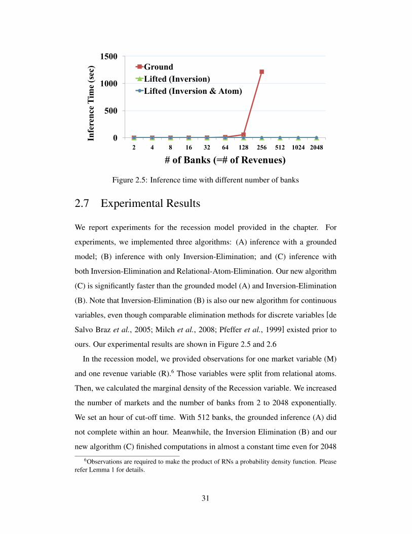
0

500

1000

1500

2 4 8 16 32 64 128 256 512 1024 2048

Infe

renc

e Ti

me

(sec

)

# of Banks (=# of Revenues)

GroundLifted (Inversion)Lifted (Inversion & Atom)

Figure 2.5: Inference time with different number of banks

2.7 Experimental Results

We report experiments for the recession model provided in the chapter. For

experiments, we implemented three algorithms: (A) inference with a grounded

model; (B) inference with only Inversion-Elimination; and (C) inference with

both Inversion-Elimination and Relational-Atom-Elimination. Our new algorithm

(C) is significantly faster than the grounded model (A) and Inversion-Elimination

(B). Note that Inversion-Elimination (B) is also our new algorithm for continuous

variables, even though comparable elimination methods for discrete variables [de

Salvo Braz et al., 2005; Milch et al., 2008; Pfeffer et al., 1999] existed prior to

ours. Our experimental results are shown in Figure 2.5 and 2.6

In the recession model, we provided observations for one market variable (M)

and one revenue variable (R).6 Those variables were split from relational atoms.

Then, we calculated the marginal density of the Recession variable. We increased

the number of markets and the number of banks from 2 to 2048 exponentially.

We set an hour of cut-off time. With 512 banks, the grounded inference (A) did

not complete within an hour. Meanwhile, the Inversion Elimination (B) and our

new algorithm (C) finished computations in almost a constant time even for 2048

6Observations are required to make the product of RNs a probability density function. Pleaserefer Lemma 1 for details.

31

0

500

1000

1500

2000

2500

2 4 8 16 32 64 128 256 512 1024 2048

Infe

renc

e Ti

me

(sec

)

# of Markets

GroundLifted (Inversion)Lifted (Inversion & Atom)

Figure 2.6: Inference time with different number of markets

banks. With 512 markets, (A) could not finish within an hour, again. With 1024

markets, (B) did not finish in an hour. Meanwhile, our new algorithm (C) finished

in a reasonable time (about 151 secs) even with 2048 markets.

2.8 Conclusion and Future work

In this chapter, we propose a new exact lifted inference algorithm for Relational

Continuous Models (RCMs). This algorithm is an advancement of exact inference

in RCMs, since all previous works are restricted to discrete domain. Given a query

and observations, our algorithm exactly computes the conditional density of the

query, when potentials satisfy specified conditions.

There are two limitations in our current algorithm. First, found potentials which

satisfy the conditions in Section 2.5 are variants of Gaussian potentials. Thus,

finding potentials beyond Gaussian is a goal of our future works. Second, the

current algorithm is designed only for continuous variables. Many real-world

models require not only continuous variables but also discrete variables. Thus,

making an efficient inference algorithm for hybrid relational models would be a

promising direction.

32

2.9 Appendix

Proof of Lemma 1 Here, we prove that the product of RNs integrates to a con-

stant given the conditions. The constant becomes the normalizing factor of the

probability density function.

We prove this by contradiction. Suppose that the product of RNs does not

integrate to a constant. That is, it integrates to infinity.

According to Equation 2.2, the product of RNs maintains the same form after

integrating out a random variable x. Thus, only possible case to be infinity is when

the marginal (after an integration over x) is a constant function of another random

variable y which is not yet integrated.

When x has relations with more than one variable (e.g. y and z), the condition

for infinity is not satisfied. The marginal includes a potential φ(y, z). When x

has a relation with only y which has relations with other variables beyond x, the

condition for infinity is not satisfied. The marginal is not a constant function of y.

Thus, only φ(x, y) satisfies the condtion for infinity. Given the assumption that

at least a RN includes a constant, y can not be a variable. Thus, it contradicts the

assumption. �

Proof of Lemma 6 First, the product of RNMs is analytically integrated by the

rule in Equation 2.3. Thus, the product of RNMs satisfy the Condition (I).

Second, the product of RNMs is closed under product operations and marginal-

izations. It satisfies the Condition (I) because it is an exponential family. That is,

the product of two RNMs (φ′RNM(x, y) and φ′′RNM(x, y)) is another RNMs (φ′′′RNM

(x, y)). Thus, the product of RNMs satisfies the Condition (II).

Third, it is also closed under marginalizations. When y j in Equation 2.4 is

33

substituted with y j − d, the following equation is derived.

ˆxi

∏y∈Y

exp(−

(xi − y − d)2

2σ2

)=

∏yi,y j∈Y

exp(−

(yi − y j − 0))2

2σ2 · |Y|

)

Thus, the result is the product of RNMs.

As explained in the proof of Theorem 5, the the product of RNMs can be rep-

resented as the following form φRNM(X, x′) · φRNM(Y, x′) when x′ is the variable

of integration.

When y j ∈ Y in Equation 2.6 is substituted with y j − d ∈ Y′, the following

equation is derived.

ˆx′φRNM(X, x′) · φRNM(Y, x′) = c ·

ˆx′φRN(X, x′) · φRN(Y′, x′)

= c′ · φ′RN(X,X) · φ′′RN(X,Y′) · φ′′′RN(Y′,Y′)

= c′′ · φ′RNM(X,X) · φ′′RNM(X,Y) · φ′′′RNM(Y,Y)

The result is also the product of RNMs. Thus, it is closed under marginalizations.

�

34

CHAPTER 3

LIFTED RELATIONAL KALMANFILTERING

Kalman filtering is a computational tool with widespread applications in robotics,

financial and weather forecasting, environmental engineering and defense. Given

observation and state transition models, the Kalman filter (KF) recursively esti-

mates the state variables of a dynamic system. However, the KF requires a cubic

time matrix inversion operation at every timestep which prevents its application in

domains with large numbers of state variables. We propose Relational Gaussian

Models to represent and model dynamic systems with large numbers of variables

efficiently. Furthermore, we devise an exact lifted Kalman filtering algorithm

which takes only linear time in the number of random variables at every timestep.

We prove that our algorithm takes linear time in the number of state variables even

when individual observations apply to each variable. To our knowledge, this is the

first lifted (linear time) algorithm for filtering with continuous dynamic relational

models.

3.1 Introduction

Many real-world systems can be modeled by continuous variables and relation-

ships (or dependences) among them. The Kalman filter (KF) [Kalman, 1960]

accurately estimates the state of a dynamic system given a sequence of control-

inputs and observations. It has been applied in a broad range of domains which

include weather forecasting [Burgers et al., 1998], localization and tracking in

robotics [Limketkai et al., 2005], economic forecasting in finance [Bahmani-

Oskooee and Brown, 2004] and many others. Given a sequence of observations

35

and Gaussian dependences between variables, the filtering problem is to calculate

the conditional probability density of the state variables at each timestep. Unfor-

tunately, the KF computations are cubic in the number of random variables which

limits current exact methods to domains with limited number of random variables.

This has led to the combination of approximation and sampling (e.g. the Ensemble

Kalman filter [Evensen, 1994]).

This chapter leverages the ability of relational languages [Friedman et al., 1999;

Poole, 2003; Milch et al., 2005; Richardson and Domingos, 2006] to specify

models with size of representation independent of the size of populations in-

volved. Various lifted inference algorithms for relational models have been pro-

posed [Poole, 2003; de Salvo Braz et al., 2005; Milch and Russell, 2006; Singla

and Domingos, 2008; Wang and Domingos, 2008; Choi et al., 2010a]. These

seek to carry computations in time independent of the size of the populations in-

volved. However, the key challenge in relational filtering (of dynamic systems)

is ensuring that the representation does not degenerate to the ground case when

multiple observation are made. As more observations are received, an increasing

number of objects become distinguished. This precludes the application of previ-

ously known algorithms unless approximately equivalent objects are grouped with

expensive clustering algorithms.

We propose Relational Gaussian Models (RGMs) to model dynamic systems

of large number of variables in a relational fashion. RGMs have as their main

building block the pairwise linear Gaussian potential as detailed in Section 3.2.

Further, we propose a new lifted filtering algorithm that is able to marginalize out

random variables of the previous timestep efficiently (in time linear in the num-

ber of random variables) while maintaining the relational (RGM) representation.

This prevents the model from being increasingly grounded even when individual

observations are made for all random variables. Moreover, updating the relational

representation takes only quadratic time in the number of relational atoms (sets

of random variables). One key insight is that, given identical observation models,

even when the means of the random variables are dispersed their variances remain

36

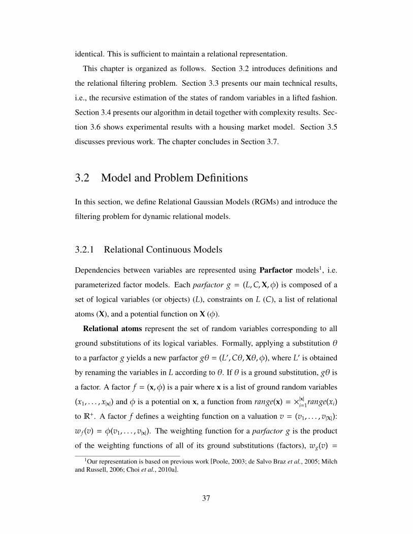
identical. This is sufficient to maintain a relational representation.

This chapter is organized as follows. Section 3.2 introduces definitions and

the relational filtering problem. Section 3.3 presents our main technical results,

i.e., the recursive estimation of the states of random variables in a lifted fashion.

Section 3.4 presents our algorithm in detail together with complexity results. Sec-

tion 3.6 shows experimental results with a housing market model. Section 3.5

discusses previous work. The chapter concludes in Section 3.7.

3.2 Model and Problem Definitions

In this section, we define Relational Gaussian Models (RGMs) and introduce the

filtering problem for dynamic relational models.

3.2.1 Relational Continuous Models

Dependencies between variables are represented using Parfactor models1, i.e.

parameterized factor models. Each parfactor g = (L,C,X, φ) is composed of a

set of logical variables (or objects) (L), constraints on L (C), a list of relational

atoms (X), and a potential function on X (φ).

Relational atoms represent the set of random variables corresponding to all

ground substitutions of its logical variables. Formally, applying a substitution θ

to a parfactor g yields a new parfactor gθ = (L′,Cθ,Xθ, φ), where L′ is obtained

by renaming the variables in L according to θ. If θ is a ground substitution, gθ is

a factor. A factor f = (x, φ) is a pair where x is a list of ground random variables

(x1, . . . , x|x|) and φ is a potential on x, a function from range(x) = ×|x|i=1range(xi)

to R+. A factor f defines a weighting function on a valuation v = (v1, . . . , v|X|):

w f (v) = φ(v1, . . . , v|x|). The weighting function for a parfactor g is the product

of the weighting functions of all of its ground substitutions (factors), wg(v) =

1Our representation is based on previous work [Poole, 2003; de Salvo Braz et al., 2005; Milchand Russell, 2006; Choi et al., 2010a].

37

∏f∈g w f (v). Hence, a set of parfactors G defines2 a probability density propor-

tional to,

wG(v) =∏g∈G

∏f∈g

w f (v). (3.1)

3.2.2 Relational Gaussian Models

Relational Gaussian Models (RGMs) are a subset of Relational Continuous

Models (RCMs) where potentials are restricted to be Gaussian distributions. RGMs

are composed of three types of parfactor models: (1) Relational Transition Mod-

els (RTMs); (2) Relational Pairwise Models (RPMs); and (3) Relational Obser-

vation Models (ROMs). Suppose that we have n relational atoms: X1t (L), . . .,

Xnt (L) where L is a list of logical variables. In a relational linear dynamic model,

relational atoms are linearly influenced by control-inputs U1t (L), . . ., Un

t (L). Sim-

ilarly, a linear observation model specifies the relationship between observation

variables O1t (L), . . ., On

t (L) and other relational atoms. Control inputs and obser-

vations are associated with relational atoms in two ways: (1) direct association;

and (2) indirect association. We provide further details in Section 3.2.4.

Relational Transition Models (RTMs) model the dependence of relational

atoms at the next timestep, X jt+1(a′), on relational atoms at the current timestep,

Xit(a), and (when available) control-input information. They take the following

form,

X jt+1(a′) = Bi, j

X · Xit(a) + Bi, j

U ·Uit(a) + Gi, j

RTM, (3.2)

where Gi, jRTM ∼ N(0, σi, j

RTM) and N(m, σ2) is the normal distribution with mean m

and variance σ2. Bi, jX and Bi, j

U are the transition models, matrices or a constants,

corresponding to two relational atoms.

For univariate state variables, we can represent the transition model with a lin-

2The condition is that at least a random variable has a prior distribution as outlined in [Choi etal., 2010a].

38

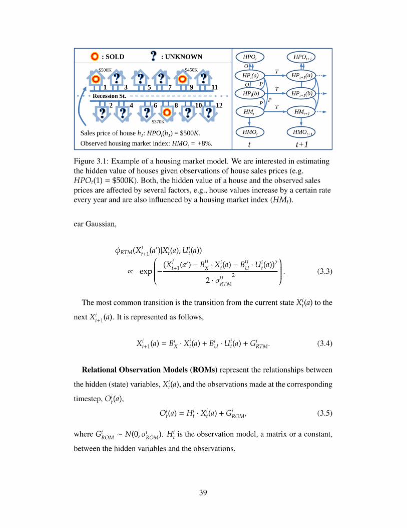
Sales price of house h1: HPOt(h1) = $500K.

Observed housing market index: HMOt = +8%.

O

O P

P P

T

T

T

t t+1

HPOt

HPt(a)

HPt(b)

HMt

HMOt

HPOt+1

HPt+1(a)

HPt+1(b)

HMt+1

HMOt+1

: UNKNOWN : SOLD

2 4 6 8 10 12

$370K

1 3 5 7 9 11

$500K $450K

Recession St. … …

Figure 3.1: Example of a housing market model. We are interested in estimatingthe hidden value of houses given observations of house sales prices (e.g.HPOt(1) = $500K). Both, the hidden value of a house and the observed salesprices are affected by several factors, e.g., house values increase by a certain rateevery year and are also influenced by a housing market index (HMt).

ear Gaussian,

φRTM(X jt+1(a′)|Xi

t(a),Uit(a))

∝ exp

− (X jt+1(a′) − Bi j

X · Xit(a) − Bi j

U ·Uit(a))2

2 · σi jRTM

2

. (3.3)

The most common transition is the transition from the current state Xit(a) to the

next Xit+1(a). It is represented as follows,

Xit+1(a) = Bi

X · Xit(a) + Bi

U ·Uit(a) + Gi

RTM. (3.4)

Relational Observation Models (ROMs) represent the relationships between

the hidden (state) variables, Xit(a), and the observations made at the corresponding

timestep, Oit(a),

Oit(a) = Hi

t · Xit(a) + Gi

ROM, (3.5)

where GiROM ∼ N(0, σi

ROM). Hit is the observation model, a matrix or a constant,

between the hidden variables and the observations.

39

Lifted Relational Kalman Filter a potential a random variable

P

P

T

T

T T

T

T

I P

P T

T I

I P

T I

I

P

P

P

1

tX

2

tX

3

tX

1

1tX

2

1tX

3

1tXMarginalizing

1

tX Marginalizing 3

tX Marginalizing 2

tX Filtered model at time t+1

P

P

P

1

1tX

2

1tX

3

1tX

Figure 3.2: This model has three relational atoms, Xi, which may represent anynumber of random variables. The relational representation dramaticallyeliminates the need for redundant potentials. Hence, representation and filteringbecome much more efficient than in the propositional case. Note that theconventional KF representation is not suited for efficient (i.e. lifted) inference.

In the linear Gaussian representation, they take the following form,

φROM(Oit(a)|Xi

t(a)) ∝ exp

− (Oit(a) −Hi

t · Xit(a))2

2 · σiROM

2

. (3.6)

Relational Pairwise Models (RPMs) represent Gaussian dependences between

pairs of relational atoms within the same timestep as follows,

Xit(a) = Ri, j

t · Xjt(a′) + Gi, j

RPM, (3.7)

where Gi, jRPM ∼ N(0, σi, j

RPM). Ri, jt is the pairwise coefficient, a matrix or a constant,

between the two relational atoms.

Note that RTMs and ROMs are directed models while RPMs are undirected.

The directed models represent the nature of dynamic systems (e.g. the state at the

next timestep depends on the current timestep). The product of RPMs is an effi-

cient way to represent a multivariate Gaussian density over all the state variables.3

3Note that a multivariate Gaussian density (of state variables) is a quadratic exponential form.The quadratic exponential form can always be decomposed into terms involving only single vari-ables and pairs of variables. We provide additional details in Section 3.5.

40

3.2.3 A Relational Filtering Problem

Given a prior (or current belief) over the state variables, the filtering problem is

to compute the posterior after a sequence of timesteps. The input to the problem

is: (1) Relational Gaussian Model (RTMs, RPMs and ROMs); (2) current be-

lief over the relational atoms (Xi0) represented by a product of relational Gaussian

potentials; (3) sequence of control-inputs (Ui1, . . . ,U

iT); and (4) sequence of obser-

vations (Oi1, . . . ,O

iT). The output is the relational Gaussian posterior distribution

over the relational atoms (XiT) at timestep T.

3.2.4 Input and Observation Association

At every timestep the control-inputs and observations must be associated with the

random variables they affect. The ideas in this section apply to control-inputs and

observations but we illustrate them for observations.

We distinguish two types of observations: direct and indirect. Direct observa-

tions are those made for a specific random variable. For instance, if we make an

observation for each random variable in a subset Ait ⊆ Xi

t of the ground substitu-

tions of relational atom Xit, we are looking at the following model,

∏a j∈Ai

t

φROM

(oi

t(a j)|Xit(a j)

). (3.8)

In the example of Figure 3.1, observing the selling price of a house would dramat-

ically reduce the variance of the hidden variable that represents the true value of

that house.

Similarly, multiple direct observations, Oit = oi,1

t , oi,2t , . . . , o

i,|Oit|

t , could be made

for each variable in some set of random variables,

∏a j∈Ai

t

∏oi,k

t ∈Oit

φROMk

(oi,k

t (a j)|Xit(a j)

). (3.9)

Given some notion of neighborhood (e.g. a residential neighborhood or a block

41

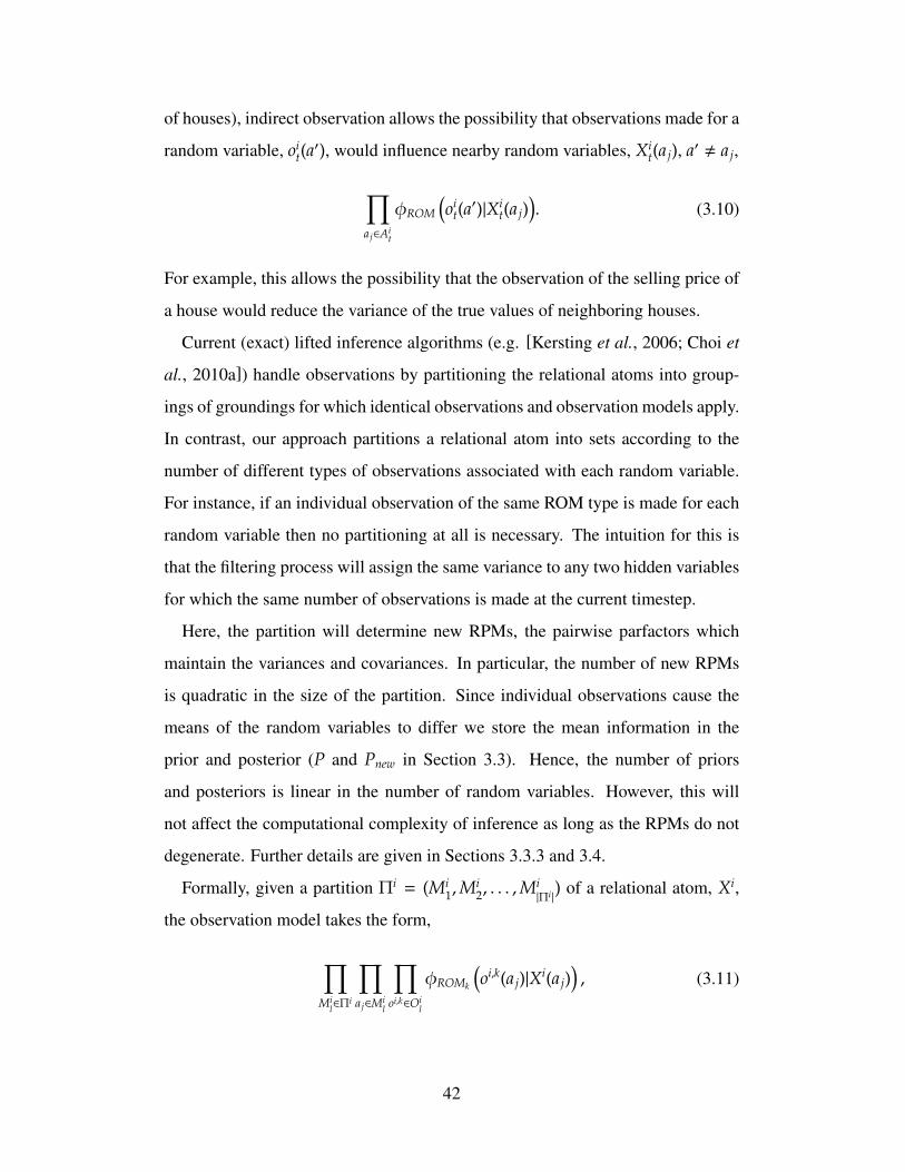
of houses), indirect observation allows the possibility that observations made for a

random variable, oit(a′), would influence nearby random variables, Xi

t(a j), a′ , a j,

∏a j∈Ai

t

φROM

(oi

t(a′)|Xi

t(a j)). (3.10)

For example, this allows the possibility that the observation of the selling price of

a house would reduce the variance of the true values of neighboring houses.

Current (exact) lifted inference algorithms (e.g. [Kersting et al., 2006; Choi et

al., 2010a]) handle observations by partitioning the relational atoms into group-

ings of groundings for which identical observations and observation models apply.

In contrast, our approach partitions a relational atom into sets according to the

number of different types of observations associated with each random variable.

For instance, if an individual observation of the same ROM type is made for each

random variable then no partitioning at all is necessary. The intuition for this is

that the filtering process will assign the same variance to any two hidden variables

for which the same number of observations is made at the current timestep.

Here, the partition will determine new RPMs, the pairwise parfactors which

maintain the variances and covariances. In particular, the number of new RPMs

is quadratic in the size of the partition. Since individual observations cause the

means of the random variables to differ we store the mean information in the

prior and posterior (P and Pnew in Section 3.3). Hence, the number of priors

and posteriors is linear in the number of random variables. However, this will

not affect the computational complexity of inference as long as the RPMs do not

degenerate. Further details are given in Sections 3.3.3 and 3.4.

Formally, given a partition Πi = (Mi1,M

i2, . . . ,M

i|Πi|

) of a relational atom, Xi,

the observation model takes the form,

∏Mi

l∈Πi

∏a j∈Mi

l

∏oi,k∈Oi

l

φROMk

(oi,k(a j)|Xi(a j)

), (3.11)

42

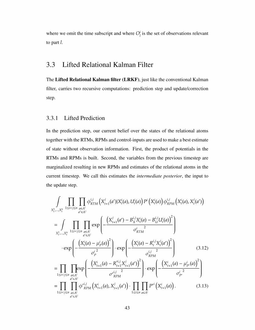
where we omit the time subscript and where Oil is the set of observations relevant

to part l.

3.3 Lifted Relational Kalman Filter

The Lifted Relational Kalman filter (LRKF), just like the conventional Kalman

filter, carries two recursive computations: prediction step and update/correction

step.

3.3.1 Lifted Prediction

In the prediction step, our current belief over the states of the relational atoms

together with the RTMs, RPMs and control-inputs are used to make a best estimate

of state without observation information. First, the product of potentials in the

RTMs and RPMs is built. Second, the variables from the previous timestep are

marginalized resulting in new RPMs and estimates of the relational atoms in the

current timestep. We call this estimates the intermediate posterior, the input to

the update step.

ˆ

X1t ,...,X

nt

∏1≤i< j≤n

∏a∈Ai

a′∈A j

φi, jRTM

(X j

t+1(a′)|Xit(a),Ui

t(a))

Pi(Xi

t(a))φi, j

RPM

(Xi

t(a),X jt(a′))

=

ˆ

X1t ,...,X

nt

∏1≤i< j≤n

∏a∈Ai

a′∈A j

exp

−(X j

t+1(a′) − Bi, jX Xi

t(a) − Bi, jU Ui

t(a))2

σiRTM

2

· exp

−(Xi

t(a) − µiP(a)

)2

σiP

2

· exp

−(Xi

t(a) − Ri, jt X j

t(a′))2

σi, jRPM

2

(3.12)

=∏

1≤i< j≤n

∏a∈Ai

a′∈A j

exp

−(Xi

t+1(a) − R′i, jt+1X jt+1(a′)

)2

σ′i, jRPM

2

· exp

−(Xi

t+1(a) − µiP′(a)

)2

σiP′

2

=

∏1≤i< j≤n

∏a∈Ai

a′∈A j

φ′i, jRPM

(Xi

t+1(a),X jt+1(a′)

)·

∏1≤i≤n

∏a∈Ai

P′i(Xi

t+1(a)). (3.13)

43

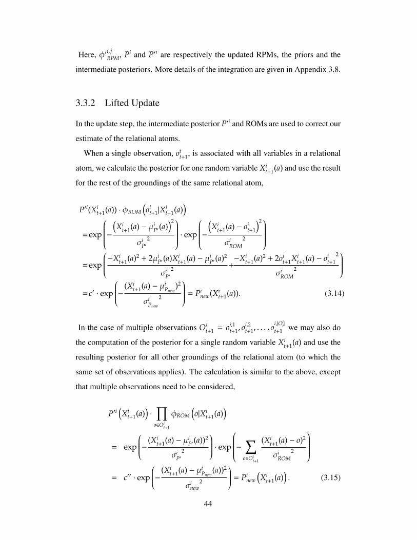
Here, φ′i, jRPM, Pi and P′i are respectively the updated RPMs, the priors and the

intermediate posteriors. More details of the integration are given in Appendix 3.8.

3.3.2 Lifted Update

In the update step, the intermediate posterior P′i and ROMs are used to correct our

estimate of the relational atoms.

When a single observation, oit+1, is associated with all variables in a relational

atom, we calculate the posterior for one random variable Xit+1(a) and use the result

for the rest of the groundings of the same relational atom,

P′i(Xit+1(a)) · φROM

(oi

t+1|Xit+1(a)

)=exp

−(Xi

t+1(a) − µiP′(a)

)2

σiP′

2

· exp

−(Xi

t+1(a) − oit+1

)2

σiROM

2

=exp

−Xit+1(a)2 + 2µi

P′(a)Xit+1(a) − µi

P′(a)2

σiP′

2 +−Xi

t+1(a)2 + 2oit+1Xi

t+1(a) − oit+1

2

σiROM

2

=c′ · exp

− (Xit+1(a) − µi

Pnew)2

σiPnew

2

= Pinew(Xi

t+1(a)). (3.14)

In the case of multiple observations Oit+1 = oi,1

t+1, oi,2t+1, . . . , o

i,|Oit|

t+1 we may also do

the computation of the posterior for a single random variable Xit+1(a) and use the

resulting posterior for all other groundings of the relational atom (to which the

same set of observations applies). The calculation is similar to the above, except

that multiple observations need to be considered,

P′i(Xi

t+1(a))·

∏o∈Oi

t+1

φROM

(o|Xi

t+1(a))

= exp

− (Xit+1(a) − µi

P′(a))2

σiP′

2

· exp

− ∑o∈Oi

t+1

(Xit+1(a) − o)2

σiROM

2

= c′′ · exp

− (Xit+1(a) − µi

Pnew(a))2

σinew

2

= Pinew

(Xi

t+1(a)). (3.15)

44

3.3.3 Lifted Inference with Individual Observations

One of the key challenges in lifted inference is handling individual observations.

Current methods ground a relational atom when different observations are made

for its random variables. It is usually the case that models shatter combinatorially

fast and thus forfeit the benefits of a relational representation and the applicability

of lifted inference.

We solve this problem in the LRKF by noting that the variances and covari-

ances in the model are not affected by individual observations. We are thus able

to represent the variances and covariances in a relational way while allowing vari-

ables to carry individual means. Further, the lifted prediction operation applies

unmodified to this representation.

Lemma 7 The variances of two random variables X(a), X(b) in an RGM are

equal after a filtering step (Lifted Prediction and Lifted Update) if the following

conditions hold before the filtering step: (1) both random variables are in the same

relational atom; (2) the variance of both variables is the same; (3) observations

are made for both variables or none of them.

Proof Given conditions (1) and (2), we first prove that the variance of both ran-

dom variables is the same after the Lifted Prediction step. Note that condition (3)

is not relevant to this step.

WLOG we assume Xt(a) and Xt(b) have different means, µt(a) and µt(b). More-

over, it is easy to see that the variance of Xit+1(a) and Xi

t+1(b) is the same after

marginalizing all random variables of timestep t due to the following two rea-

sons: (i) X(a) and X(b) are in the same relational atom and thus share the same

relationships with other random variables; (ii) the means are not involved in the

marginalizations (see Section 3.3.1). It follows that we can represent the potentials

45

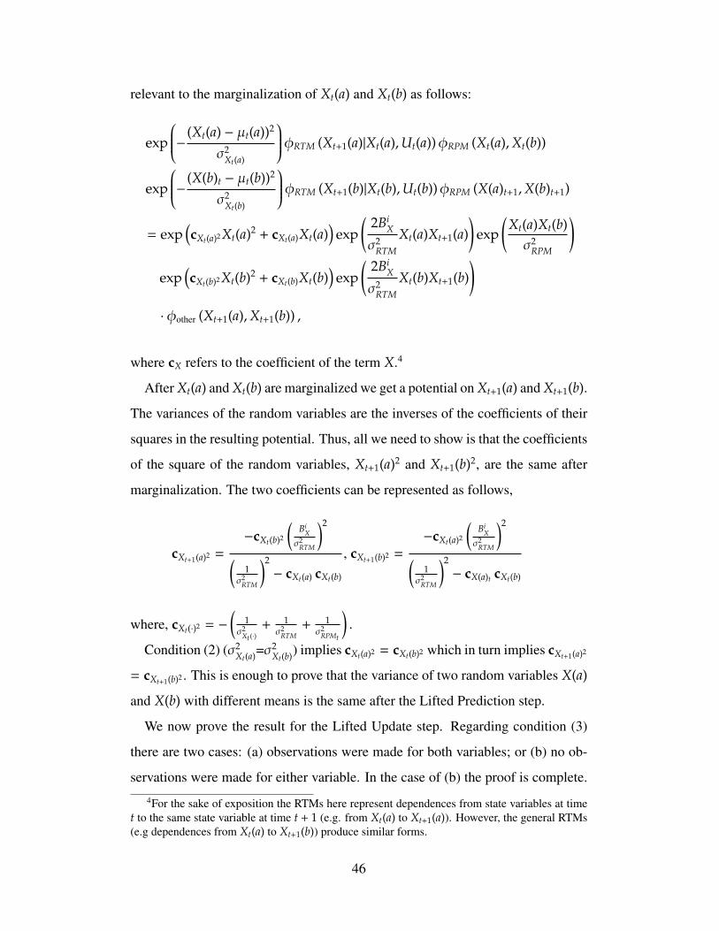
relevant to the marginalization of Xt(a) and Xt(b) as follows:

exp

− (Xt(a) − µt(a))2

σ2Xt(a)

φRTM (Xt+1(a)|Xt(a),Ut(a))φRPM (Xt(a),Xt(b))

exp

− (X(b)t − µt(b))2

σ2Xt(b)

φRTM (Xt+1(b)|Xt(b),Ut(b))φRPM (X(a)t+1,X(b)t+1)

= exp(cXt(a)2Xt(a)2 + cXt(a)Xt(a)

)exp

(2Bi

X

σ2RTM

Xt(a)Xt+1(a))

exp(

Xt(a)Xt(b)σ2

RPM

)exp

(cXt(b)2Xt(b)2 + cXt(b)Xt(b)

)exp

(2Bi

X

σ2RTM

Xt(b)Xt+1(b))

· φother (Xt+1(a),Xt+1(b)) ,

where cX refers to the coefficient of the term X.4

After Xt(a) and Xt(b) are marginalized we get a potential on Xt+1(a) and Xt+1(b).

The variances of the random variables are the inverses of the coefficients of their

squares in the resulting potential. Thus, all we need to show is that the coefficients

of the square of the random variables, Xt+1(a)2 and Xt+1(b)2, are the same after

marginalization. The two coefficients can be represented as follows,

cXt+1(a)2 =−cXt(b)2

(Bi

Xσ2

RTM

)2

(1

σ2RTM

)2

− cXt(a) cXt(b)

, cXt+1(b)2 =−cXt(a)2

(Bi

Xσ2

RTM

)2

(1

σ2RTM

)2

− cX(a)t cXt(b)

where, cXt(·)2 = −(

1σ2

Xt(·)+ 1

σ2RTM

+ 1σ2

RPMt

).

Condition (2) (σ2Xt(a)=σ

2Xt(b)) implies cXt(a)2 = cXt(b)2 which in turn implies cXt+1(a)2

= cXt+1(b)2 . This is enough to prove that the variance of two random variables X(a)

and X(b) with different means is the same after the Lifted Prediction step.

We now prove the result for the Lifted Update step. Regarding condition (3)

there are two cases: (a) observations were made for both variables; or (b) no ob-

servations were made for either variable. In the case of (b) the proof is complete.

4For the sake of exposition the RTMs here represent dependences from state variables at timet to the same state variable at time t + 1 (e.g. from Xt(a) to Xt+1(a)). However, the general RTMs(e.g dependences from Xt(a) to Xt+1(b)) produce similar forms.

46

In the case of (a), the update step for X(a) can be represented by,

exp

− (Xt+1(a) − µXt+1(a))2

σ2Xt+1(a)i

−(Xt+1(a) − oat)

2

σXROM2

= exp

− (Xt+1(a) − µ+Xt+1

(a))2

σ+Xt+1(a)2

where,

σ+2Xt+1(a) =

σ2Xt+1(a)σ

2XROM

σ2Xt+1(a)i + σ2

XROM

, µ+Xt+1(a) =

σ2XROM

µXt+1(a) + σ2Xt+1(a)oat

σ2XROM

+ σ2Xt+1(a)

Likewise, after the update step the variance of X(b) is,

σ+2Xt+1(b) =

σ2Xt+1(b)iσ

2XROM

σ2Xt+1(b)i + σ2

XROM

By condition (2) and the proof for the prediction step, σXt+1(a)i = σXt+1(b)i . Thus,

σ+Xt+1(a) = σ+

Xt+1(b). �

Lemma 8 The covariances of two pairs of variables (X(a), X(b)) and (X(a), X(c))

in an RGM are equal after a filtering step (Lifted Prediction and Lifted Update)

if the following conditions hold before the filtering step: (1) the three random

variables are in the same relational atom; (2) the covariance of both pairs of

variables is the same; (3) observations are made for the three variables or none

of them.

Proof The method used in the proof of Lemma 7 can be employed in this proof:

The terms involving the individual observations do not affect terms which deter-

mine the covariance of two random variables. �

3.4 Algorithms and Computational Complexity

Let X (|X|) be the set (number) of all random variables in the model and X =

(X1, . . . ,X|X|) be the set of relational atoms (also, a partition of X). In this section

we speak of the relational atoms as sets of random variables.

47

Figure 3.3 presents our Lifted Relational Kalman filtering algorithm. The inputs

to the algorithm are: relational atoms, X; the RGM, RTMs MX, RPMs MP and

ROMs MO; the prior over the relational atoms, P0; and the control-inputs, U[1,...,T],

and observations, O[1,...,T], for each timestep.

The algorithm computes the posterior recursively. Split partitions the domains

of each relational atom Xi as induced by the control-inputs Ut. Lifted Predict cal-

culates new RPMs, MP5, and intermediate posterior, Pint, based on the transition

models, MX, and the control-inputs, Ut. Then, Split Obs partitions the domains

of each relational atom Xi as induced by the observations, Oit. Lifted Update

calculates the new posterior, Pcur, based on the intermediate posterior, Pint, the

observation models, MO, and the observations, Oit.

Given the control-inputs, Split partitions relational atoms as done in previous

work: e.g. Split [Poole, 2003] and SHATTER [de Salvo Braz et al., 2005]. If

the control-inputs are allowed to differ for the variables in a relational atom, the

model will be propositionalized. Hence, there is little advance in how we handle

individual control-inputs with respect to previous algorithms [Choi et al., 2010a].6

Algorithm Split Obs partitions a relational atom Xi based on the observations.

However, Split Obs will only partition a relational atom in case the conditions

of Lemmas 7 and 8 do not hold, i.e., when different number of observations are

made for the relational variables. If the conditions of Lemmas 7 and 8 hold,

the efficiency of the relational representation will be preserved even if multiple

observations are made for all variables in some or all of the relational atoms.

Lemma 9 The complexity of Lifted Predict is O(|X| · |Xt+ |2). Where Xt+ is the

set of relational atoms output by Split.

Proof This step corresponds to the marginalization (Equation (3.13) and Ap-

5In our representation the number of relational atoms determines the number of RPMs whichis equal to E(|X|, 2) (the number of 2-combinations of |X| with repetition).

6However, we conjecture that techniques similar to the ones we used for ROMs can be appliedto RTMs. Any two random variables in the same atom will have the same variance after theLifted Predict step if they receive the same types of control inputs. That is, RTMs of the sametype will increase the variances of the random variables by the same amount.

48

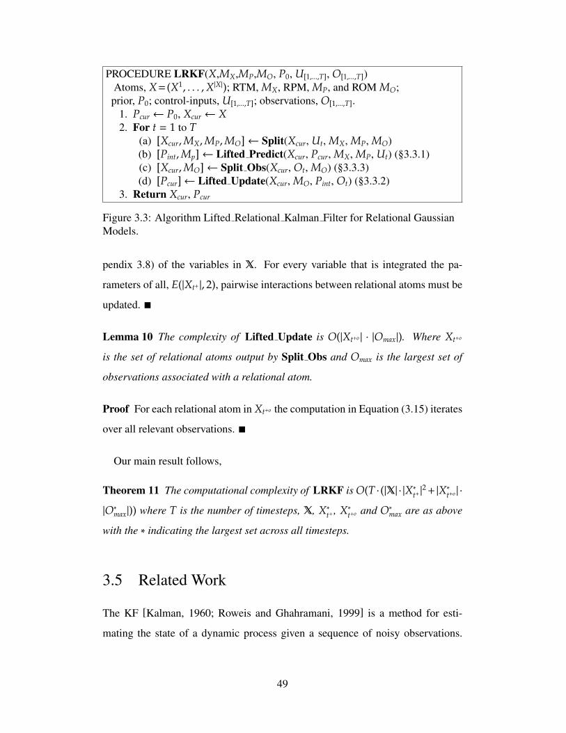
PROCEDURE LRKF(X,MX,MP,MO, P0, U[1,...,T], O[1,...,T])Atoms, X= (X1, . . . ,X|X|); RTM, MX, RPM, MP, and ROM MO;prior, P0; control-inputs, U[1,...,T]; observations, O[1,...,T].

1. Pcur← P0, Xcur← X2. For t = 1 to T

(a) [Xcur,MX,MP,MO]← Split(Xcur, Ut, MX, MP, MO)(b) [Pint,Mp]← Lifted Predict(Xcur, Pcur, MX, MP, Ut) (§3.3.1)(c) [Xcur,MO]← Split Obs(Xcur, Ot, MO) (§3.3.3)(d) [Pcur]← Lifted Update(Xcur, MO, Pint, Ot) (§3.3.2)

3. Return Xcur, Pcur

Figure 3.3: Algorithm Lifted Relational Kalman Filter for Relational GaussianModels.

pendix 3.8) of the variables in X. For every variable that is integrated the pa-

rameters of all, E(|Xt+ |, 2), pairwise interactions between relational atoms must be

updated. �

Lemma 10 The complexity of Lifted Update is O(|Xt+o | · |Omax|). Where Xt+o

is the set of relational atoms output by Split Obs and Omax is the largest set of

observations associated with a relational atom.

Proof For each relational atom in Xt+o the computation in Equation (3.15) iterates

over all relevant observations. �

Our main result follows,

Theorem 11 The computational complexity of LRKF is O(T · (|X| · |X∗t+ |2 + |X∗t+o | ·

|O∗max|)) where T is the number of timesteps, X, X∗t+ , X∗t+o and O∗max are as above

with the ∗ indicating the largest set across all timesteps.

3.5 Related Work

The KF [Kalman, 1960; Roweis and Ghahramani, 1999] is a method for esti-

mating the state of a dynamic process given a sequence of noisy observations.

49

It is restricted to linear dynamic and linear measurement models both with ad-

ditive Gaussian noise. The Extended Kalman filter (EKF) [Sorenson and Stub-

berud, 1968] extends the KF to non-linear systems. For high dimensional data, a

sampling method has been devised, the Ensemble Kalman filter [Evensen, 1994].

Exact Kalman filtering for high dimensional data is not feasible because exact fil-

tering requires matrix inversions which take time cubic in the number of random

variables.

Our RGMs represent the probability density as a product of node and edge

factors. Any multivariate Gaussian is a quadratic exponential and can thus be

written in this form. This is related to the information form of the Gaussian den-

sity and is the basis of other models such as Directed Gaussian Models (DGMs)

[Cowell, 1998] and Gaussian Markov Random Fields (GMRFs) [Rue and Held,

2005]. However, RGMs are relational while DGMs and GMRFs are not. Thus,

the previous models do not have a compact (relational) representations and, more

importantly, an efficient (lifted) exact inference algorithm.

Relational probabilistic models allow the specification of models with size in-

dependent of the sizes of the populations in the model [Friedman et al., 1999;

Poole, 2003; Milch et al., 2005; Richardson and Domingos, 2006]. Lifted infer-

ence algorithms [de Salvo Braz et al., 2005; Milch and Russell, 2006] attempt to

carry as much of the computations without propositionalizing the model. [Poole,

2003], solves inference problems by dynamically splitting and unifying sets of

ground atoms. [de Salvo Braz et al., 2005] (FOVE) introduced counting elimi-

nation to efficiently eliminate atoms with different parameterizations. [Milch et

al., 2008] (C-FOVE) take a slightly different approach with the introduction of

counting formulas. However, all of the above lifted inference algorithms are not

applicable to models with continuous variables.

[Kersting et al., 2006] introduced Logical HMMs that combine ideas from Sta-

tistical Relational Learning and dynamic models. Indeed their work, as ours,

pursues the benefits that the relational approach brings to inference and learning.

However, their work is inherently discrete and further, they assume specific tran-

50

sition and observation models.

For relational models with continuous variables, recent advances have made

inference possible. [Wang and Domingos, 2008] is an approximate algorithm

based on sampling, search and local optimization. [Choi et al., 2010a] is an exact

variable elimination algorithm for continuous domains. The latter algorithm is

similar to the marginalization problem that is part of the prediction step in filtering.

However, none of these algorithms have been devised with dynamic models in

mind nor do they address the problem of individual observations.

3.6 Experimental Results

We compare the average filtering time of LRKF and a conventional Kalman filter

by varying the number of random variables. We implemented both the LRKF and

the conventional KF (which handles random variables individually) in Perl. This

makes the manipulation of the dynamically changing structure convenient.

For the housing market model in Figure 3.1, we randomly choose the parame-

ters of the models (priors, RTMs, RPMs, and ROMs) and provide observations for

HMOt and HPOt(·). To emphasize the difference in scalability, we assume that

some set of houses has individual observations in each timestep, HPOt(·), while

the rest of the houses do not. We ran the two filters over 50 timesteps. The results

in graph 3.4 confirm our theoretical results contrasting the linear time complexity

of LRKF with the cubic time complexity of the Kalman filter.

3.7 Conclusion

We propose Relational Gaussian Models to represent and model dynamic systems

in a relational (first-order) way. Further, we present the first algorithm for filtering

or tracking at the first-order level. Our theoretical analysis and empirical tests

show that our approach leads to significant gains in efficiency and enables filtering

51

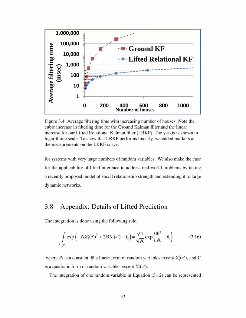
1

10

100

1,000

10,000

100,000

1,000,000

0 200 400 600 800 1000

Aver

age

filte

ring

tim

e (m

sec)

Number of houses

Ground KFLifted Relational KF

Figure 3.4: Average filtering time with increasing number of houses. Note thecubic increase in filtering time for the Ground Kalman filter and the linearincrease for our Lifted Relational Kalman filter (LRKF). The y-axis is shown inlogarithmic scale. To show that LRKF performs linearly, we added markers atthe measurements on the LRKF curve.

for systems with very large numbers of random variables. We also make the case

for the applicability of lifted inference to address real-world problems by taking

a recently proposed model of social relationship strength and extending it to large

dynamic networks.

3.8 Appendix: Details of Lifted Prediction

The integration is done using the following rule,

ˆ

Xit(a∗)

exp(−AXi

t(a∗)

2+ 2BXi

t(a∗) − C

)=

√π√A

exp(B2

A− C

). (3.16)

whereA is a constant, B a linear form of random variables except Xit(a∗), and C

is a quadratic form of random variables except Xit(a∗).

The integration of one random variable in Equation (3.12) can be represented

52

as follows,

ˆ

Xit(a∗)

∏1≤ j≤n

∏a′∈A j

exp

−(X j

t+1(a′) − Bi, jX Xi

t(a∗) − Bi, j

U Uit(a∗))2

σiRTM

2

exp

−(Xi

t(a∗) − µi

P(a∗))2

σiP

2

· exp

−(Xi

t(a∗) − Ri, j

t X jt(a′))2

σi, jRPM

2

(3.17)

=

ˆ

Xit(a∗)

exp

−AXit(a∗)

2+

c +∑

1≤ j≤n

∑a′∈A j

c jtX

jt(a′) + c j

t+1X jt+1(a′)

Xit(a∗) − C

=

ˆ

Xit(a∗)

exp

−AXit(a∗)

2+

c +∑

1≤ j≤n

c jt

∑a′∈A j

X jt(a′) + c j

t+1

∑a′∈A j

X jt+1(a′)

Xit(a∗)− C

=

ˆ

Xit(a∗)

exp

−AXit(a)

2+

c +∑

1≤ j≤n

c jtX

jt + c j

t+1Xjt+1

Xit(∗a) − C

, (3.18)

when c, c jt and c j

t+1 represent constants calculated from Equation (3.17), and X jt

represents∑

a′∈A j X jt(a′).

Note the quadratic form in Equation (3.16) includes the following types of ex-

pression,

(X +X′)2 = [X2] + 2[XX] + 2XX′ + [X′2] + 2[X′X′], (3.19)

where [X2] is∑

a∈A X(a)2, and [XX] is∑

a,a′∈A,a,a′ X(a)X(a′).

53

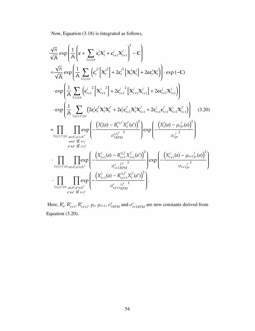
Now, Equation (3.18) is integrated as follows,

√π√A

exp

1A

c +∑

1≤ j≤n

c jtX

jt + c j

t+1Xjt+1

2

− C

=

√π√A

exp

1A

∑1≤ j≤n

(c j

t

2[X

jt

2]

+ 2c jt

2 [X

jtX

jt

]+ 2cc j

tXjt

) · exp (−C)

· exp

1A

∑1≤ j≤n

(c j

t+1

2[X

jt+1

2]

+ 2c jt+1

2 [X

jt+1X

jt+1

]+ 2cc j

t+1Xjt+1

)· exp

1A

∑1≤ j< j′≤n

(2c j

tcj′

t XjtX

j′

t + 2c jtc

j′

t+1XjtX

j′

t+1 + 2c jt+1c j′

t+1Xjt+1X

j′

t+1

) (3.20)

=∏

1≤ j< j′≤n

∏a∈A j,a′∈A j′

a,a∗ if i= ja′,a∗ if i= j′

exp

−(Xi

t(a) − R′ j, j′

t X j′

t (a′))2

σ′tj, j′

RPM

2

exp

−(X j

t(a) − µtjP′(a)

)2

σtjP′

2

·

∏1≤ j< j′≤n

∏a∈A j,a′∈A j′

exp

−(X j

t+1(a) − R′ j, j′

t+1 X j′

t+1(a′))2

σ′t+1j, j′

RPM

2

exp

−(X j

t+1(a) − µt+1jP′(a)

)2

σt+1jP′

2

·

∏1≤ j, j′≤n

∏a∈A j,a′∈A j′

a′,a∗ if i= j′

exp

−(X j

t+1(a) − R′ j, j′

t,t+1X j′

t (a′))2

σ′t,t+1j, j′

RPM

2

.Here, R′t, R′t+1, R′t,t+1, µt, µt+1, σ′tRPM and σ′t+1RPM are new constants derived from

Equation (3.20).

54

CHAPTER 4

LIFTED INFERENCE WITH AGGREGATEFACTORS

Aggregate factors (that is, those based on aggregate functions such as SUM, AV-

ERAGE, AND etc) in probabilistic relational models can compactly represent de-

pendencies among a large number of relational random variables. However, propo-

sitional inference on a factor aggregating n k-valued random variables into an r-

valued result random variable is O(rk2n). Lifted methods can ameliorate this to

O(rnk) in general and O(rk log n) for commutative associative aggregators. In

this chapter, I propose (a) an exact solution constant in n when k=2 for certain

aggregate operations such as AND, OR and SUM, and (b) a close approximation

for inference with aggregate factors with time complexity constant in n. This

approximate inference involves an analytical solution for some operations when

k>2. The approximation is based on the fact that the typically used aggregate

functions can be represented by linear constraints in the standard (k−1)-simplex

in Rk where k is the number of possible values for random variables. This in-

cludes even aggregate functions that are commutative but not associative (e.g.,

the MODE operator that chooses the most frequent value). Our algorithm takes

polynomial time in k (which is only 2 for binary variables) regardless of r and n,

and the error decreases as n increases. Therefore, for most applications (in which

a close approximation suffices) our algorithm is a much more efficient solution

than existing algorithms. I present experimental results supporting these claims.

I also present a (c) third contribution which further optimizes aggregations over

multiple groups of random variables with distinct distributions.

55

4.1 Introduction

Relational models can compactly (that is, intensionally) represent graphical mod-

els involving a large number of random variables, each of them representing a rela-

tion between objects in a domain [Koller and Pfeffer, 1997; Friedman et al., 1999;

Milch et al., 2005; Richardson and Domingos, 2006].

While it is possible to take advantage of compactness only for representation

and expand the model into a propositional (extensional) form for inference, lifted

inference methods try to keep the representation as compact as possible even

during inference, increasing efficiency [Poole, 2003; de Salvo Braz et al., 2007;

Milch et al., 2008; Singla and Domingos, 2008].

The first proposed lifted inference solutions could deal only with factors on a

fixed number of random variables. Aggregate parametric factors (based on aggre-

gate functions such as OR, MAX, AND, SUM, AVERAGE, MODE and MEDIAN),

which are defined on a varying, intensionally defined set of random variables,

still needed to be treated propositionally, with cost exponential in the number n

of random variables. [Kisynski and Poole, 2009] introduced lifted methods for

aggregate factors that reduce this complexity to O(rk log n) for commutative as-

sociative aggregate functions on n k-valued random variables being aggregated

into an r-valued random variable (and even O(rk) for OR and MAX)1. However,

for general cases (such as the non-associative function MODE), their exact infer-

ence method has time O(rnk), that is, polynomial in n.

The contributions of this chapter are threefold. I contribute an exact solution

constant in n when k = 2 for aggregate operations AND, OR, MAX and SUM. I

also present an efficient (constant in n) approximate algorithm for inference with

aggregate factors, for all typical aggregate functions. The potential of a aggregate

factor for a valuation v of a set of random variables depends only on the histogram

on the distribution of k values in V (in what [Milch et al., 2008] calls a counting

1Note that r=n for aggregate functions such as SUM of n binaray variables.

56

formula). I show that the typical aggregate functions but for XOR2 can be repre-

sented by linear constraints in the space of histograms (a (k−1)-simplex). Because

aggregate factors’ potentials on the space of histograms can be approximated by a

normal distribution, one can approximately sums over them (which is the main in-

ference operation) by computing the volume under normal distributions truncated

by linear constraints. This holds even for MODE, which is commutative but not

associative.

This approximation can be computed analytically for all operations on binary

random variables and for certain operations on multivalued (k>2) random vari-

ables such as SUM and MEDIAN. Otherwise, it is computed by Gibbs sampling

with a limited number of iterations [Geweke, 1991; Damien and Walker, 2001].

Finally, a third contribution is a further optimization for aggregations of multiple

groups of random variables, each with its own distribution.

This chapter is organized as follows. Section 4.2 defines relational models and

our inference problem, AFM (Aggregation Factor Marginalization). Section 4.3

presents our lifted inference methods for aggregate factors followed by an ex-

tended algorithm for the generalized problems in Section 4.4. Section 4.5 pro-

vides the error bounds of the approximations. I present some empirical results in

Section 4.6. The chapter concludes in Section 4.7.

4.2 Background and Problem Definition

This chapter is concerned about inference problems over relational models with

aggregate factors. I now revisit these concepts.

4.2.1 First-order Probabilistic Models

A factor f is a pair (A f , φ f ) where A f is a tuple of random variables and φ f is a

potential function from the range of A f to the nonnegative real numbers. Given a

2XOR has its own simple solution.

57

valuation v of random variables (rvs), the potential of f on v is w f (v) = φ f (A f ).

The joint probability defined by a set F of factors on a valuation v of random

variables is the normalization of∏

f∈F w f (v). If each factor in F is a conditional

probability of a child random variable given the value of its parent random vari-

ables, and there are no directed cycles in the graph formed by directed edges from

parents to children, then the model defines a Bayesian network. Otherwise it is an

undirected model.

One can have parameterized (indexed) random variables by using predicates,

which are functions mapping parameter values (indices) to random variables. A

relational atom is an application of a predicate, possibly with free variables. For

example, a predicate f riends is used in atoms f riends(X,Y), f riends(X, bob) and

f riends( john, bob), where X and Y are free variables and john and bob possible

parameter values. f riends( john, bob) is a ground atom and directly corresponds

to a random variable.

A parfactor is a tuple (L,C,A, φ) composed of a set of parameters (also called

logical variables) L, a constraint C on L, a tuple of atoms A, and a potential

function φ. Let a substitution θ be an assignment to L and Aθ the relational

atom (possibly ground) resulting from replacing logical variables by their values

in θ. A parfactor g stands for the set of factors gr(g) with elements (Aθ, φ) for

every assignment θ to the parameters L that satisfies the constraint C. A First-

order Probabilistic Model (FOPM) is a compact, or intensional, representation

of a graphical model. It is composed by a domain, which is the set of possible

parameter values (referred to as domain objects) and a set of parfactors. The

corresponding graphical model is the one defined by all instantiated factors. The

joint probability of a valuation v according to a set of parfactors G is

P(v) = 1/Z∏g∈G

∏f∈gr(g)

w f (v), (4.1)

where Z is a normalization constant.

Example: The dependence between political ads and votes in the example in

58

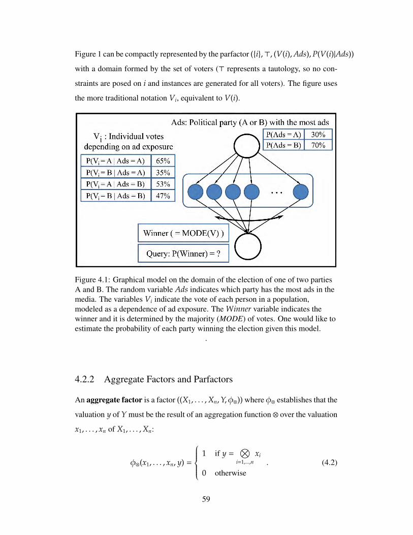
Figure 1 can be compactly represented by the parfactor ({i},>, (V(i),Ads),P(V(i)|Ads))

with a domain formed by the set of voters (> represents a tautology, so no con-

straints are posed on i and instances are generated for all voters). The figure uses

the more traditional notation Vi, equivalent to V(i).

Figure 4.1: Graphical model on the domain of the election of one of two partiesA and B. The random variable Ads indicates which party has the most ads in themedia. The variables Vi indicate the vote of each person in a population,modeled as a dependence of ad exposure. The Winner variable indicates thewinner and it is determined by the majority (MODE) of votes. One would like toestimate the probability of each party winning the election given this model.

.

4.2.2 Aggregate Factors and Parfactors

An aggregate factor is a factor ((X1, . . . ,Xn,Y, φ⊗)) where φ⊗ establishes that the

valuation y of Y must be the result of an aggregation function ⊗ over the valuation

x1, . . . , xn of X1, . . . ,Xn:

φ⊗(x1, . . . , xn, y) =

1 if y =

⊗i=1,...,n

xi

0 otherwise. (4.2)

59

This chapter considers the aggregate functions OR, MAX, AND, XOR, SUM, AV-

ERAGE, MODE and MEDIAN. Noisy versions such as Noisy-OR can be repre-

sented by adding an extra factor on xi.3

An aggregate parfactor g = (L,C,X,⊗,Y), where X and Y are now relational

atoms, can be used by FOPMs to compactly represent a set of aggregate factors.

The set gr(g) of ground factors instantiated from g comprises the aggregate fac-

tors ((Xθ0θ1, . . . ,Xθ0θn,Yθ0), φ⊗), for each substitution θ0 on the logical vari-

ables in Y consistent with constraint C, and substitutions θ1, . . . , θn on the logical

variables in X but not in Y consistent with C. For the example in Figure 1, the

conditional probability of Winner can be compactly represented by the aggregate

parfactor (i,>,V(i),MODE,Winner). More general aggregation cases (for ex-

ample, with aggregated random variables sets including more than one predicate)

can be normalized to this type of aggregated parfactor, as detailed in [Kisynski

and Poole, 2009].

4.2.3 Inference with Aggregate Parfactors: Aggregate FactorMarginalization (AFM)

This section is concerned about the inference problem of marginalizing a set of rvs

in an FOPM with aggregate factors to determine the marginal density of others. As

shown by [Kisynski and Poole, 2009], this can be done by using C-FOVE [Milch

et al., 2008] extended with a lifted operation for summing random variables out of

an aggregate parfactor. These summations can be reduced to the Aggregate Factor

Marginalization (AFM) calculation:

φ′y(y) =∑x1,,xn

φ⊗(y, x1, . . . , xn)∏

1≤i≤n

φx(xi)

.3Our definitions are based on [Kisynski and Poole, 2009] but differ from theirs in this aspect;

while our aggregate factors are deterministic, theirs include an extra potential for noisy versions.As explained, one can do the same with an extra factor/parfactor.

60

where φx is the (same for all i) potential product of all other factors in the model

that have Xi as an argument, and φ′y is the resulting potential on y alone. This sub-

problem is also one that needs to be solved in extending Lifted Belief Propagation

[Singla and Domingos, 2008] to deal with aggregate factors.

[Kisynski and Poole, 2009] shows how, when different xi have different po-

tential functions on them, the problem can be normalized (by splitting and using

auxiliary variables) to multiple such sums in which this uniformity holds. Simi-

larly, one can separate the case in which only some xi need to be summed out into

two different aggregate parfactors, one for all aggregate random variables being

summed out, and another for the remaining ones.

A direct computation of AFM is exponential in n. [Kisynski and Poole, 2009]

shows lifted operations that can be done in time polynomial or logarithmic in n

(depending on certain conditions explained below). In Section 4.3 I present two

lifted methods, one exact and one approximate, with time constant in n.

4.2.4 Inference Problems with Inequality

This section defines aggregate factors with inequality constraints by using

φ⊗≤(y, x1, . . . , xn) =

1 if y ≤ x1 ⊗ · · · ⊗ xn

0 otherwise

with the corresponding problem AFM[≤] defined as

∑x1,...,xn

φ⊗≤(y, x1, . . . , xn) ·∏

1≤i≤n

φx(xi)

.φ⊗≥ and AFM[≥] are defined analogously.

61

4.2.5 Existing Methods for AFM Problems

MAX and its special case OR (as well as their noisy versions) allow factorizations

leading to lifted marginalization constant in n [Dıez and Galan, 2003]. These

operators can be decomposed into the product of n potentials:4

∑x1,...,xn

φ⊗(y, x1, . . . , xn) ·n∏

i=1

φx(xi) =∑

y′

∑x1,...,xn

n∏i=1

φy′,y(y′, y) · φy′,x(y′, xi)

(4.3)

=∑

y′

φy′,y(y′, y)n∏

i=1

∑xi

φy′,x(y′, xi)

.(4.4)

Because the product is over a term independent of n, one can compute it once and

exponentiate in time constant in n:

=∑

y′

φy′,y(y′, y)

∑x′φy′,x(y′, x′)

n .For other aggregate functions that happen to be commutative and associative,

AFM can be computed by a recursive decomposition [Kisynski and Poole, 2009]

into a subproblem with half the number of aggregated random variables, and there-

fore in time O(r2k log n) when n is a power of 2:

∑x1,...,xn

φ⊗(y, x1, . . . , xn)n∏

i=1

φx(xi) =∑

y=y′⊗y′′

∑x1,...,x n

2

φ⊗(y′, x1, . . . , x n2)

n2∏

i=1

φx(xi)

·

∑x n

2 +1,...,xn

φ⊗(y′′, x n2 +1, . . . , xn)

n∏i= n

2 +1

φx(xi)

,4See [Dıez and Galan, 2003] for details on φy′,y and φy′,x.

62

where φ⊗(y, xi) =

1 if y = xi

0 otherwise.

Note that the two decomposition halves are the same problem up to variable re-

naming and thus computed in time O(k log n), r2 times (once per value of y′ or

y′′ and another per value of y). [Kisynski and Poole, 2009] describes the minor

adjustments needed when n is not a power of 2.

4.3 Efficient Methods for AFM Problems

This section now presents solutions for AFM problems. The exact solutions pre-

sented in the previous section are efficient. However, their applicability is limited

to some operations [Dıez and Galan, 2003], or their computational complexity

still depends on the number of rvs [Kisynski and Poole, 2009]. Here, it proposes

an exact solution for some cases, and new efficient approximate marginalizations

that are applicable to more aggregate functions.

4.3.1 Normal Distribution with Linear Constraints

[Kisynski and Poole, 2009] shows how the potential of an aggregate parfactor de-

pends only on the value histogram of its aggregated random variables (histograms

were introduced in Counting Elimination [de Salvo Braz et al., 2007] and used as

counting formulas in [Milch et al., 2008]).

Given values x1, . . . , xn for n rvs with the same range, the value histogram of x

is a vector h with hu = |{i : xi = u}| for each u in the rvs’ range. When a potential

function on x1, . . . , xn depends on the histogram alone, as in the case of aggre-

gate factors, then there is a function φh on histograms such that φ(y, x1, . . . , xn) =

φh(y, h) and φ⊗(y, x1, . . . , xn) = φ⊗h(y, h). In what follows, this section de-

scribes the binomial case (range of xi equal to 2) for clarity, but it applies to the

63

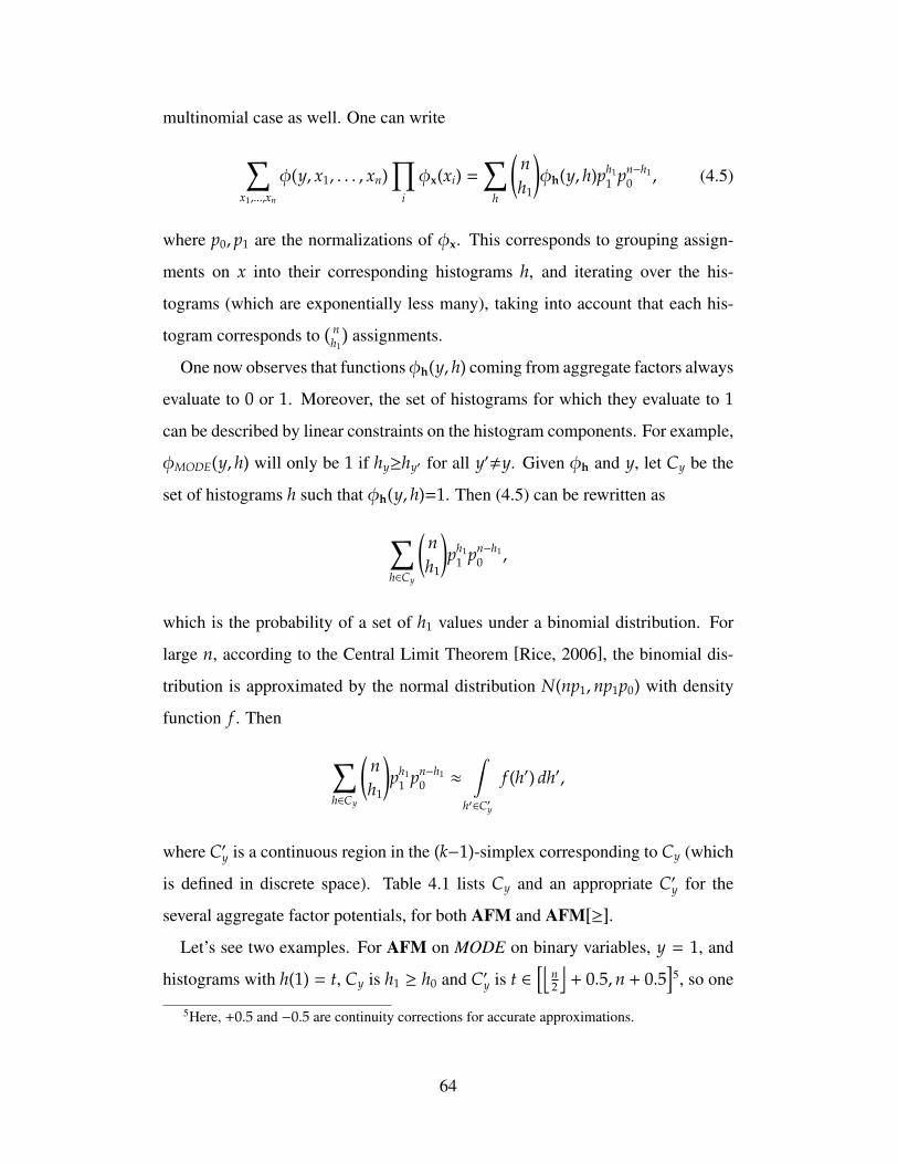
multinomial case as well. One can write

∑x1,...,xn

φ(y, x1, . . . , xn)∏

i

φx(xi) =∑

h

(nh1

)φh(y, h)ph1

1 pn−h10 , (4.5)

where p0, p1 are the normalizations of φx. This corresponds to grouping assign-

ments on x into their corresponding histograms h, and iterating over the his-

tograms (which are exponentially less many), taking into account that each his-

togram corresponds to( n

h1

)assignments.

One now observes that functionsφh(y, h) coming from aggregate factors always

evaluate to 0 or 1. Moreover, the set of histograms for which they evaluate to 1

can be described by linear constraints on the histogram components. For example,

φMODE(y, h) will only be 1 if hy≥hy′ for all y′,y. Given φh and y, let Cy be the

set of histograms h such that φh(y, h)=1. Then (4.5) can be rewritten as

∑h∈Cy

(nh1

)ph1

1 pn−h10 ,

which is the probability of a set of h1 values under a binomial distribution. For

large n, according to the Central Limit Theorem [Rice, 2006], the binomial dis-

tribution is approximated by the normal distribution N(np1,np1p0) with density

function f . Then

∑h∈Cy

(nh1

)ph1

1 pn−h10 ≈

ˆ

h′∈C′y

f (h′) dh′,

where C′y is a continuous region in the (k−1)-simplex corresponding to Cy (which

is defined in discrete space). Table 4.1 lists Cy and an appropriate C′y for the

several aggregate factor potentials, for both AFM and AFM[≥].

Let’s see two examples. For AFM on MODE on binary variables, y = 1, and

histograms with h(1) = t, Cy is h1 ≥ h0 and C′y is t ∈[⌊

n2

⌋+ 0.5,n + 0.5

]5, so one

5Here, +0.5 and −0.5 are continuity corrections for accurate approximations.

64

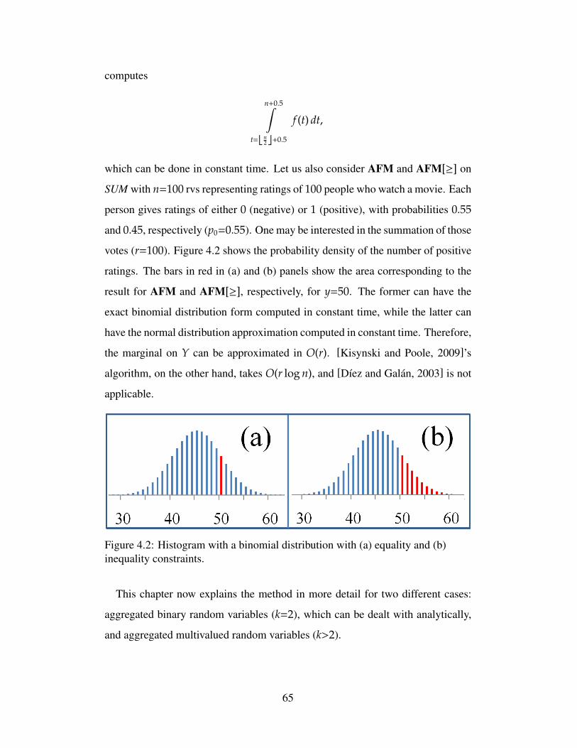
computes

n+0.5ˆ

t=b n2c+0.5

f (t) dt,

which can be done in constant time. Let us also consider AFM and AFM[≥] on

SUM with n=100 rvs representing ratings of 100 people who watch a movie. Each

person gives ratings of either 0 (negative) or 1 (positive), with probabilities 0.55

and 0.45, respectively (p0=0.55). One may be interested in the summation of those

votes (r=100). Figure 4.2 shows the probability density of the number of positive

ratings. The bars in red in (a) and (b) panels show the area corresponding to the

result for AFM and AFM[≥], respectively, for y=50. The former can have the

exact binomial distribution form computed in constant time, while the latter can

have the normal distribution approximation computed in constant time. Therefore,

the marginal on Y can be approximated in O(r). [Kisynski and Poole, 2009]’s

algorithm, on the other hand, takes O(r log n), and [Dıez and Galan, 2003] is not

applicable.

Figure 4.2: Histogram with a binomial distribution with (a) equality and (b)inequality constraints.

This chapter now explains the method in more detail for two different cases:

aggregated binary random variables (k=2), which can be dealt with analytically,

and aggregated multivalued random variables (k>2).

65

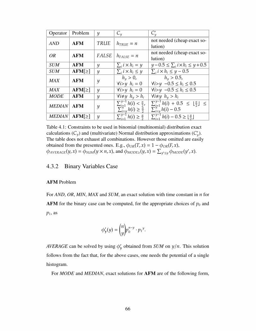
Operator Problem y Cy C′y

AND AFM TRUE hTRUE = n not needed (cheap exact so-lution)

OR AFM FALSE hFALSE = n not needed (cheap exact so-lution)

SUM AFM y∑

i i × hi = y y−0.5 ≤∑

i i×hi ≤ y+0.5SUM AFM[≥] y

∑i i × hi ≤ y

∑i i × hi ≤ y − 0.5

MAX AFM y hy > 0,∀i>y hi = 0

hy > 0.5,∀i>y −0.5 ≤ hi ≤ 0.5

MAX AFM[≥] y ∀i>y hi = 0 ∀i>y −0.5 ≤ hi ≤ 0.5MODE AFM y ∀i,y hy > hi ∀i,y hy > hi

MEDIAN AFM y∑y−1

i=1 h(i) < n2 ,∑n

i=y h(i) ≥ n2

∑y−1i=1 h(i) + 0.5 ≤ bn

2 c ≤∑ni=y h(i) − 0.5

MEDIAN AFM[≥] y∑y−1

i=1 h(i) ≥ n2

∑y−1i=1 h(i) − 0.5 ≥ bn

2 c

Table 4.1: Constraints to be used in binomial (multinomial) distribution exactcalculations (Cy) and (multivariate) Normal distribution approximations (C′y).The table does not exhaust all combinations. However those omitted are easilyobtained from the presented ones. E.g., φOR(T, x) = 1 − φOR(F, x),φAVERAGE(y, x) = φSUM(y × n, x), and φMODE≥(y, x) =

∑y′≤y φMODE(y′, x).

4.3.2 Binary Variables Case

AFM Problem

For AND, OR, MIN, MAX and SUM, an exact solution with time constant in n for

AFM for the binary case can be computed, for the appropriate choices of p0 and

p1, as

φ′y(y) =

(ny

)pn−y

0 · p1y.

AVERAGE can be solved by using φ′y obtained from SUM on y/n. This solution

follows from the fact that, for the above cases, one needs the potential of a single

histogram.

For MODE and MEDIAN, exact solutions for AFM are of the following form,

66

with time linear in n:

φ′y(TRUE) =

n∑i=b n

2c+1

(ni

)pn−i

0 · p1i.

Such solutions are more expensive because they measure the density of a re-

gion of histograms. They can be approximated by the Normal distribution in the

following way:

φ′y(TRUE) ≈

n+0.5ˆ

t=b n2c+0.5

exp(−

(t−np1)2

2·np1(1−p1)

)√

2π · np1(1 − p1)dt.

Note that MODE is not solved by either [Dıez and Galan, 2003]’s factorization

or [Kisynski and Poole, 2009]’s logarithmic algorithm, while our approach can

compute an approximation in constant time. For n is 100, p1 = 0.45, the exact

solution is about 0.18272. Our approximate solution is about 0.18286. Thus, the

error is less than 0.1% of the exact solution.

AFM[≤] and AFM[≥] Problems

For binary aggregated random variables, these problems are different from AFM

only for the SUM (and thus, AVERAGE) case. For SUM one can use the approxi-

mation

φ′y(y) =

n∑i=y

(ni

)pi

1(1 − p1)n−i≈

n+0.5ˆ

t=y−0.5

exp(−

(t−np1)2

2·np1(1−p1)

)√

2π · np1(1 − p1)dt.

4.3.3 Multivalued Variables Case

In the multivalued (k>2) case, there is a need to compute the probability of a

linearly constrained region of histograms, which motivates us to consider approx-

imate solutions with the multivariate Normal distribution. Consider the following

67

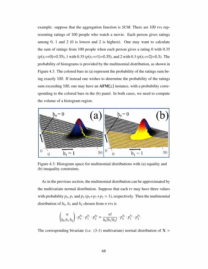
example: suppose that the aggregation function is SUM. There are 100 rvs rep-

resenting ratings of 100 people who watch a movie. Each person gives ratings

among 0, 1 and 2 (0 is lowest and 2 is highest). One may want to calculate

the sum of ratings from 100 people when each person gives a rating 0 with 0.35

(p(xi=r0)=0.35), 1 with 0.35 (p(xi=r1)=0.35), and 2 with 0.3 (p(xi=r2)=0.3). The

probability of histograms is provided by the multinomial distribution, as shown in

Figure 4.3. The colored bars in (a) represent the probability of the ratings sum be-

ing exactly 100. If instead one wishes to determine the probability of the ratings

sum exceeding 100, one may have an AFM[≥] instance, with a probability corre-

sponding to the colored bars in the (b) panel. In both cases, we need to compute

the volume of a histogram region.

Figure 4.3: Histogram space for multinomial distributions with (a) equality and(b) inequality constraints.

As in the previous section, the multinomial distribution can be approximated by

the multivariate normal distribution. Suppose that each rv may have three values

with probability p0, p1 and p2 (p0+p1+p2 = 1), respectively. Then the multinomial

distribution of h0, h1 and h2 chosen from n rvs is(n

h0 h1 h2

)· ph0

0 · ph11 · p

h22 =

n!h0!h1!h2!

· ph00 · p

h11 · p

h22 .

The corresponding bivariate (i.e. (3-1) multivariate) normal distribution of X =

68

[h0 h1] chosen from n rvs is as follows (Note that h2 = n − h1 − h2),

1(2π)2/2|Σ|1/2

· exp(−

12

(X − µ)Σ−1(X − µ)′),

when the µ and Σ are

µ = [np0 np1], Σ =

np0(1 − p0) np1p2

np2p1 np2(1 − p2)

.

Analytical Solution for Operators with a Single Linear Constraint

As in the previous section, one sets p0, p1 and p2 as 0.35, 0.35 and 0.3 respectively

and y as 100. Any operator with a single linear constraint (e.g. AFM, AFM[≤]

and AFM[≥] on SUM, and AFM[≤] and AFM[≥] on MEDIAN) allows an an-

alytical solution because there is a linear transformation from X = [h0 h1] to y.

Consider the following linear transform y = 0·h0 + 1·h1 + 2·h2 = 200 − 2·h0 − h1.

When one represents the transform as y = AX + B, the new distribution of y is

given by the 1-D Normal distribution:

1√2πΣy

· exp(−

(y−µy)2

2Σy

),

where µy = Aµ + B and Σy = AΣAT are scalars. From the transformation the

solution of AFM for y=100 can be calculated in the following way:

1√2πΣy

100+0.5ˆ

y=100−0.5

exp(−

(y−µy)2

2Σy

)dy.

The solutions of AFM[≤] and AFM[≥] for y=100 can be calculated in similar

ways.

69

Sampling for Remaining Operators

In general, integration of a multivariate truncated normal does not allow an an-

alytical solution. Fortunately, efficient Gibbs sampling methods (e.g. [Geweke,

1991; Damien and Walker, 2001]) are applicable to the truncated normal in straight-

forward ways, even with several linear constraints. This immediately feeds to an

approximation with time complexity not depending on n, the number of rvs.

4.4 Aggregate Factor with Multiple Atoms

This section now considers a generalized situation. Previous sections assume that

all rvs in a relational atom have the same distribution. Here, it deals with the

issue of aggregating J distinct groups of random variables, each represented by a

relational atom X j with n j groundings and a distinct potential φxj , for 1≤ j≤J.

y =⊗1< j<J1<i<n j

x j,i.

This problem, AFM-M, is an extension of the AFM. The AFM-M is to calcu-

late a marginal

∑x1,1,···,xJ,nJ

φ⊗(y, x1,1, · · · , xJ,nJ )J∏

j=1

∏1≤i≤n j

φxj(x j,i).

One approach is to compute an aggregate y0j per atom j, and then combine each

pair yij and yi

j+1 into yi+1b j/2c until they are all aggregated. This will have complexity

O(J log J) but works only for associative operators. For non-associative operators,

one may need to calculate the marginal for each X j independently:

∑h1,···,hJ

φ⊗h(y,h)

(n1

h11

)ph1

01,0p

h11

1,1· · ·

(nJ

hJ1

)p

hJ0

J,0phJ

1J,1

,

70

where p j,0 and p j,1 are the normalization of φxj(0) and φxj(1); h j is a histogram

for atom j, and h is the combined histogram. The complexity of this approach is

O(exp(J)).

Another approach is to make use of the representation of the aggregation opera-

tor as a set of linear constraints (Table 4.1). Note that h j is approximately Normal

when n j is large, and hi and h j are independent when i, j. Thus, the all-group his-

togram vector h is also approximately Normal distributed because it is the Normal

sum (hi =∑

j h ji ).

Any linear constraint in Table 4.1 can be re-expressed as a linear constraint

using elements of h, and the multinomial-Normal approximation can be used to

yield a similar approximate solution in time constant n, the total number of rvs.

For example, for binary random variables, the Normal approximation of the

all-group histogram is:

N

J∑j=1

n jp j,1,J∑

j=1

n jp j,1p j,0

.This way, the time complexity is only O(J) instead of O(J log J) (or O(exp(J))

for non-associative operators).

4.5 Error Analysis

Here, this section discusses error bounds for the multinomial-Normal approxima-

tions. In general, the Berry-Esseen theorem [Esseen, 1942] gives an upper bound

on the error. Suppose that φy(y) and φy(y) represent the probability mass of a

binomial distribution and density of its normal approximation, respectively. Fur-

thermore, one may represent the cumulative probabilties as Φy(y) and Φy(y)6.

Then, given any y, the error between the two cumulative probabilities is bounded

[Esseen, 1942]:

6That is, Φy(y) =y∑

i=0φy(i), and Φy(y) =

y

t=−∞φy(t) dt.

71

∣∣∣Φy(y) − Φy(y)∣∣∣ < c ·

p2 + (1 − p)2√np(1 − p)

,

where c is a small (< 1) constant. Thus, the asymptotic error bound is O(1/√

n),

and this extends to probability on any interval.

For k-valued multinomials, suppose that ΦY(A) and ΦY(A) represent the prob-

ability of a multinomial distribution and its multivariate normal approximation

over a measurable convex set A in Rk. Then, the approximation error is bounded

[Gotze, 1991]:

supA

∣∣∣ΦY(A) − ΦY(A)∣∣∣ < c ·

k√

n,

where c depends only on the multinomial parameters and not on n. In our problem,

A is determined by linear constraints, hence is convex. Thus, the asymptotic error

bound is O(k/√

n).

4.6 Experimental Results

This section provides experimental results on the example in Figure 1 (which

uses the MODE aggregate function) which give us an insight on when to use the

approximate algorithm instead of the generally applicable exact algorithm based

on Counting Formulas (the logarithmic method in [Kisynski and Poole, 2009]

does not apply to MODE).

One may compute the utility of any of the methods tested, approximations or

exact inference alike, in the following manner. One assumes a typical application

in which the utility of an error is an inverse quadratic function U(err) = 1 − err2.

The utility of a method obtaining error err is normalized by the time t it takes to

run, so U(err, t) = U(err)/t. For sampling methods, t is the time to convergence.

Finally, it plots the ratio between the utility of our methods and the utility of the

exact inference method.

Therefore, a method is advantageous over the exact inference method when this

72

ratio is greater than 1.

Figure 4.4: Ratios of utilities of approximate algorithms and exact method(histogram based counting).

An experiments runs on the approximations and the exact inference algorithm

for the model in Figure 4.1. For k = 2, it runs both the analytical and the sampling

method. Given k and n, it randomly chooses the potentials, and records the error

and the convergence time. Then, it average them over 100 trials to calculate the

utility, UApprox.

As shown in Figure 4.4, the suggested approximate algorithm has much higher

utility than the exact method for larger k and n. However, when k = 2 (binary

variables), the exact method has higher utility than sampling for relatively large n

(e.g. n = 10240). In this case, one can use the efficient analytic integration which

applies for k = 2. I also show in Figure 4.5 how the error decreases for different

values of k and n.

In addition, the results observed that the convergence time stays flat for various

k and n. However, the error of sampling method is noticeable for small n. For

example, when k = 4, the error is 3.07% with n = 40 and 1.82% with n = 80. For

larger n, this issue is resolved. The error becomes less than 1% when n = 320 and

negligible when n > 5120. These observations are consistent for various k from 2

to 6.

73

Figure 4.5: Error curves for different values of k and n.

4.7 Conclusion

Processing aggregate parfactors efficiently is an important problem since they in-

volve functions commonly used in writing models. Our contribution adds efficient

exact methods for the binary case k=2, as well as efficient approximations for the

cases in which the sets of aggregated variables are large, which is precisely the

situation in which one may be more likely to use aggregate factors in the first

place. It will therefore be an important part of practical applications of relational

graphical models.

74

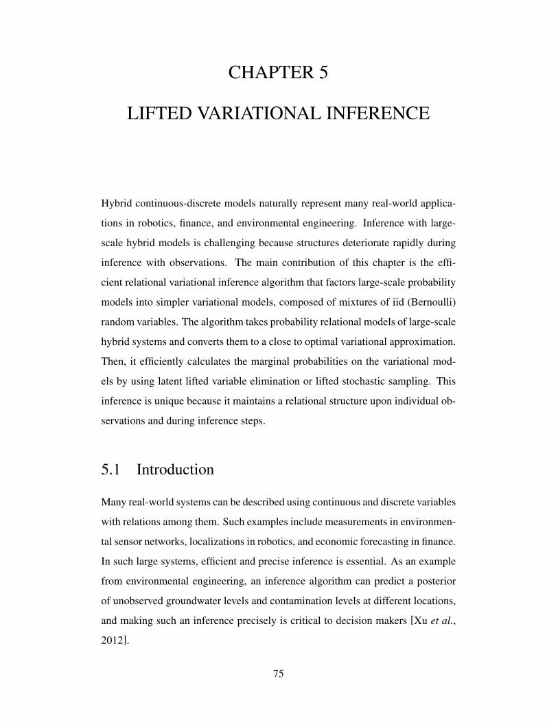
CHAPTER 5

LIFTED VARIATIONAL INFERENCE

Hybrid continuous-discrete models naturally represent many real-world applica-

tions in robotics, finance, and environmental engineering. Inference with large-

scale hybrid models is challenging because structures deteriorate rapidly during

inference with observations. The main contribution of this chapter is the effi-

cient relational variational inference algorithm that factors large-scale probability

models into simpler variational models, composed of mixtures of iid (Bernoulli)

random variables. The algorithm takes probability relational models of large-scale

hybrid systems and converts them to a close to optimal variational approximation.

Then, it efficiently calculates the marginal probabilities on the variational mod-

els by using latent lifted variable elimination or lifted stochastic sampling. This

inference is unique because it maintains a relational structure upon individual ob-

servations and during inference steps.

5.1 Introduction

Many real-world systems can be described using continuous and discrete variables

with relations among them. Such examples include measurements in environmen-

tal sensor networks, localizations in robotics, and economic forecasting in finance.

In such large systems, efficient and precise inference is essential. As an example

from environmental engineering, an inference algorithm can predict a posterior

of unobserved groundwater levels and contamination levels at different locations,

and making such an inference precisely is critical to decision makers [Xu et al.,

2012].

75

Real-world systems have large numbers of variables including both discrete

and continuous. Probabilistic first order languages, e.g. [Bacchus, 1990; Halpern,

1990; Ng and Subrahmanian, 1992; Pfeffer et al., 1999; Friedman et al., 1999;

Poole, 2003; Richardson and Domingos, 2006], describe probability distributions

at a relational level with the purpose of capturing the structure of larger models. A

key challenge of inference procedures with the languages is that they often result

in intermediate density functions involving many random variables and complex

relationship among them.

Lifted inference presently can address discrete models and continuous models,

but not hybrid ones. For (d-valued) discrete variables, lifted inference can take an

advantage of the insight which groups equivalent models into a histogram repre-

sentation with an order of poly(d) entries [de Salvo Braz et al., 2005; Milch and

Russell, 2006; Jha et al., 2010] (instead of exp(d) entries in traditional ground

models). For Gaussian potentials, lifted inference can use an insight which en-

ables maintaining compact covariance matrices during (and after) inference, e.g.

[Choi et al., 2010a].

Unfortunately, these principles are not applicable to general (non-Gaussian) hy-

brid models because the histogram is not applicable to continuous domains with-

out discretizations, and the covariance matrix is a special structure for Gaussians.

Thus, existing variational methods, e.g. NP-BLOG [Carbonetto et al., 2005] and

Latent Tree Models [Zhang, 2002; Choi et al., 2011d], focus only on discrete or

Gaussian models.

In this chapter, we present pragmatic algorithms based on a new insight (re-

lational variational-inference lemmas) which accurately factors densities of rela-

tional models into mixtures of iid random variables. These lemmas enable us

to build a variational approximation algorithm, which takes large-scale graphical

models with hybrid variables and finds close to optimal relational variational mod-

els. Then, our inference algorithms, the variable elimination and the stochastic

sampling, efficiently solve marginal inference problems on the variational mod-

els. We show that the algorithm gives a better solution than previous ones.

76

This chapter is organized as follows. Section 5.2 defines Relational Hybrid

Models. Section 5.3 presents a theoretical background, de Finetti’s theorem. Sec-

tion 5.4 overviews our Lifted Relational Variational Inference algorithm. Sec-

tion 5.5 and 5.6 respectively elucidate the learning and inference algorithms. Sec-

tion 5.7 presents our theoretical contributions, relational-variational lemmas.

Section 5.8 compares our method with existing inference methods. Section 5.9

shows experimental results, followed by the conclusion and future work in Sec-

tion 5.10.

5.2 Relational Hybrid Models (RHMs)

A factor f = (A f , φ f ) is a pair, composed of a tuple of random variables (rvs) A f

and a potential function φ f . Here, φ f is an unnormalized probability density from

the range of A f to the nonnegative real numbers. The range of a rv is discrete or

continuous, i.e., hybrid domains. Given a valuation v of rvs, the potential of f

on v is w f (v) = φ f (A f ).

We define parameterized (indexed) rvs by using predicates those are func-

tions mapping parameter values to rvs. A relational atom (or just atom) denotes

a parametrized rv with free parameter variable(s). For example, an atom X(a) can

be mapped to one of n rvs {X(a1), · · ·,X(an)} when the free parameter variable a is

substituted by a value ai.

A parfactor g = [PV,Ag, φg] is a tuple composed of parameter variables PV,

a tuple of relational atoms Ag and a potential function φg. A substitution θ is an

assignment to PV, and Agθ the relational atom (possibly ground) resulting from

replacing the logical variables by their values in θ. gr(g) is a set of factors derived

from the parfactor g by substitutions.

77

For example, a RHM can include the following parfactor:

[ (a, b)

Parameter

variables

, (X(a),Y(b))

Relational

atoms

,N(X(a)−Y(b);µ, σ2)

A potential

(linear Gaussian)

]. (5.1)

The domains of the parameter variables (a and b) can be {a1, . . . , an} and {b1, . . . , bm}.

Thus, any substitution (e.g. a = ai, b = b j) let two rvs (e.g. X(ai), Y(bj)) holds the

linear Gaussian relationship.

A Relational Hybrid Model (RHM) is a compact, or intensional, representa-

tion of graphical models with discrete and continuous rvs. An RHM is composed

of a domain, the set of possible parameter values, and a set of parfactors G. The

joint probability of an RHM G on a valuation v of rvs is as follows:

1z

∏g∈G

∏f∈gr(g)

w f (v)

where z is the normalizing constant.

This representation seems rather straightforward. However, inference proce-

dures often result in complex models. For example, eliminating X(a1) in Equation

(5.1) makes all other rvs fully connected. An important property in RHMs is

that the ground rvs mapped from a relational atom are exchangeable, defined as

follows:

Definition 1 (Exchangeable Random Variables) A sequence X(a1), · · ·,X(an) of

rvs is exchangeable, when for any finite permutation π() of the indices the joint

probability distribution of the permuted sequence X(aπ(1)), · · ·,X(aπ(n)) is the same

as the joint probability distribution of the original sequence.

Note that RHMs may include atoms with non-exchangeable rvs.1 In this case, our

variational algorithm grounds, or shatters, any atom including non-exchangeable

1Lifted inference for non-exchangeable rvs is out of scope of this chapter. Instead, see [Jha etal., 2010; Apsel and Brafman, 2011].

78

….

….

….

….

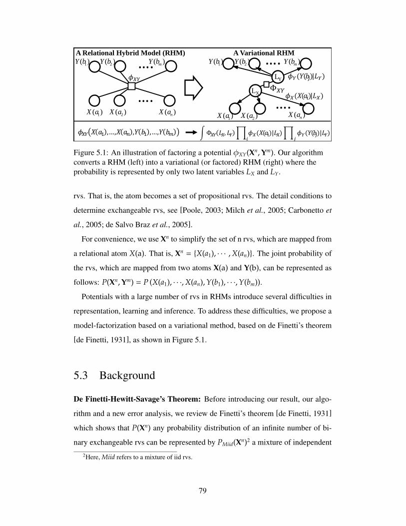
1( )X a 2( )X a )( nX a1( )X a 2( )X a )( nX a

1( )Y b 2( )Y b )( mY b 1( )Y b 2( )Y b )( mY b

A Relational Hybrid Model (RHM) A Variational RHM

Φ𝑋𝑌 𝐿𝑋, 𝐿𝑌 𝜙𝑋(𝑋(𝑎𝑖)|𝐿𝑋)𝑖

𝜙𝑌(𝑌(𝑏𝑗)|𝐿𝑌)𝑗

Φ𝑋𝑌 𝜙𝑋(𝑋(𝑎𝑖)|𝐿𝑋)

𝜙𝑌(𝑌(𝑏𝑗)|𝐿𝑌) LY

LX

𝜙𝑋𝑌

𝜙𝑋𝑌 𝑋 𝑎1 ,…,𝑋 𝑎𝑛 ,𝑌 𝑏1 ,…,𝑌 𝑏𝑚

Figure 5.1: An illustration of factoring a potential φXY(Xn,Ym). Our algorithmconverts a RHM (left) into a variational (or factored) RHM (right) where theprobability is represented by only two latent variables LX and LY.

rvs. That is, the atom becomes a set of propositional rvs. The detail conditions to

determine exchangeable rvs, see [Poole, 2003; Milch et al., 2005; Carbonetto et

al., 2005; de Salvo Braz et al., 2005].

For convenience, we use Xn to simplify the set of n rvs, which are mapped from

a relational atom X(a). That is, Xn = {X(a1), · · · ,X(an)}. The joint probability of

the rvs, which are mapped from two atoms X(a) and Y(b), can be represented as

follows: P(Xn,Ym) = P (X(a1), · · ·,X(an),Y(b1), · · ·,Y(bm)).

Potentials with a large number of rvs in RHMs introduce several difficulties in

representation, learning and inference. To address these difficulties, we propose a

model-factorization based on a variational method, based on de Finetti’s theorem

[de Finetti, 1931], as shown in Figure 5.1.

5.3 Background

De Finetti-Hewitt-Savage’s Theorem: Before introducing our result, our algo-

rithm and a new error analysis, we review de Finetti’s theorem [de Finetti, 1931]

which shows that P(Xn) any probability distribution of an infinite number of bi-

nary exchangeable rvs can be represented by PMiid(Xn)2 a mixture of independent

2Here, Miid refers to a mixture of iid rvs.

79

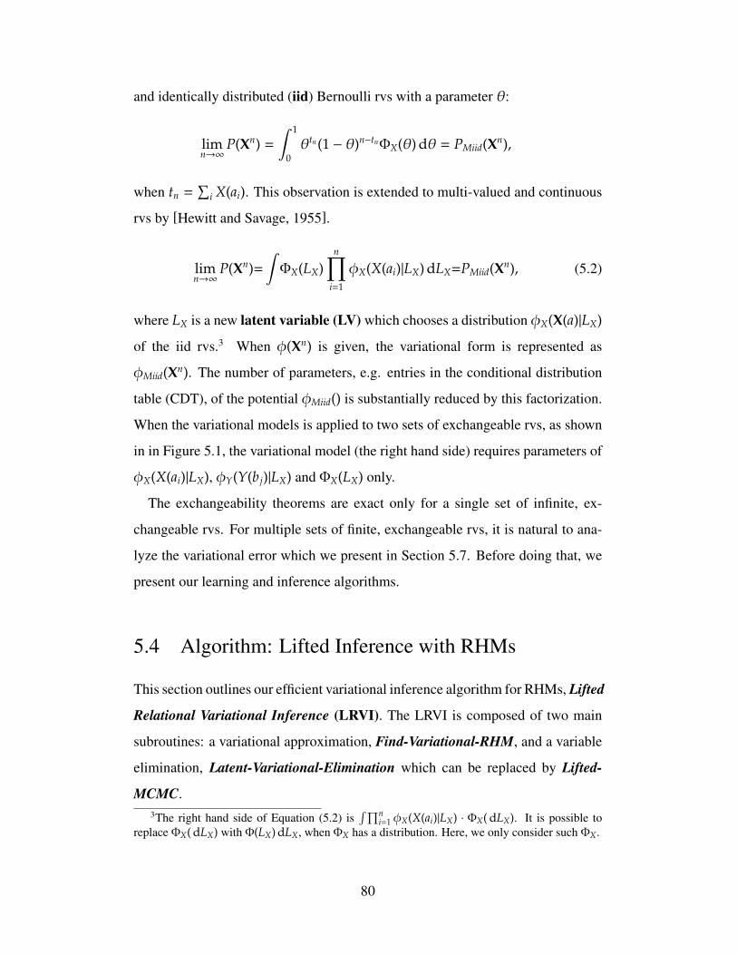
and identically distributed (iid) Bernoulli rvs with a parameter θ:

limn→∞

P(Xn) =

ˆ 1

0θtn(1 − θ)n−tnΦX(θ) dθ = PMiid(Xn),

when tn =∑

i X(ai). This observation is extended to multi-valued and continuous

rvs by [Hewitt and Savage, 1955].

limn→∞

P(Xn)=ˆ

ΦX(LX)n∏

i=1

φX(X(ai)|LX) dLX=PMiid(Xn), (5.2)

where LX is a new latent variable (LV) which chooses a distribution φX(X(a)|LX)

of the iid rvs.3 When φ(Xn) is given, the variational form is represented as

φMiid(Xn). The number of parameters, e.g. entries in the conditional distribution

table (CDT), of the potential φMiid() is substantially reduced by this factorization.

When the variational models is applied to two sets of exchangeable rvs, as shown

in in Figure 5.1, the variational model (the right hand side) requires parameters of

φX(X(ai)|LX), φY(Y(b j)|LX) and ΦX(LX) only.

The exchangeability theorems are exact only for a single set of infinite, ex-

changeable rvs. For multiple sets of finite, exchangeable rvs, it is natural to ana-

lyze the variational error which we present in Section 5.7. Before doing that, we

present our learning and inference algorithms.

5.4 Algorithm: Lifted Inference with RHMs

This section outlines our efficient variational inference algorithm for RHMs, Lifted

Relational Variational Inference (LRVI). The LRVI is composed of two main

subroutines: a variational approximation, Find-Variational-RHM, and a variable

elimination, Latent-Variational-Elimination which can be replaced by Lifted-

MCMC.3The right hand side of Equation (5.2) is

´∏ni=1 φX(X(ai)|LX) · ΦX( dLX). It is possible to

replace ΦX( dLX) with Φ(LX) dLX, when ΦX has a distribution. Here, we only consider such ΦX.

80

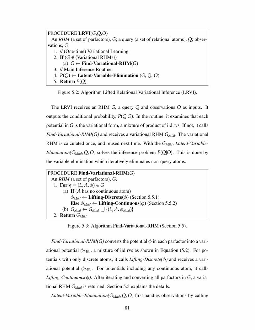
PROCEDURE LRVI(G,Q,O)An RHM (a set of parfactors), G; a query (a set of relational atoms), Q; obser-

vations, O.1. // (One-time) Variational Learning2. If (G < {Variational RHMs})

(a) G← Find-Variational-RHM(G)3. // Main Inference Routine4. P(Q)← Latent-Variable-Elimination (G, Q, O)5. Return P(Q)

Figure 5.2: Algorithm Lifted Relational Variational Inference (LRVI).

The LRVI receives an RHM G, a query Q and observations O as inputs. It

outputs the conditional probability, P(Q|O). In the routine, it examines that each

potential in G is the variational form, a mixture of product of iid rvs. If not, it calls

Find-Variational-RHM(G) and receives a variational RHM GMiid. The variational

RHM is calculated once, and reused next time. With the GMiid, Latent-Variable-

Elimination(GMiid,Q,O) solves the inference problem P(Q|O). This is done by

the variable elimination which iteratively eliminates non-query atoms.

PROCEDURE Find-Variational-RHM(G)An RHM (a set of parfactors), G.1. For g = (L,A, φ) ∈ G

(a) If (A has no continuous atom)φMiid← Lifting-Discrete(φ) (Section 5.5.1)Else φMiid← Lifting-Continuous(φ) (Section 5.5.2)

(b) GMiid← GMiid⋃{(L,A, φMiid)}

2. Return GMiid

Figure 5.3: Algorithm Find-Variational-RHM (Section 5.5).

Find-Variational-RHM(G) converts the potential φ in each parfactor into a vari-

ational potential φMiid, a mixture of iid rvs as shown in Equation (5.2). For po-

tentials with only discrete atoms, it calls Lifting-Discrete(φ) and receives a vari-

ational potential φMiid. For potentials including any continuous atom, it calls

Lifting-Continuous(φ). After iterating and converting all parfactors in G, a varia-

tional RHM GMiid is returned. Section 5.5 explains the details.

Latent-Variable-Elimination(GMiid,Q,O) first handles observations by calling

81

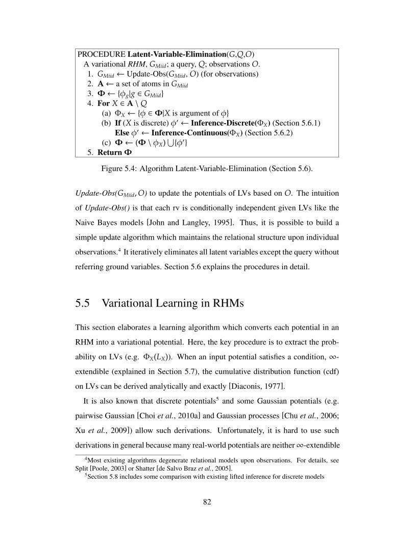
PROCEDURE Latent-Variable-Elimination(G,Q,O)A variational RHM, GMiid; a query, Q; observations O.1. GMiid← Update-Obs(GMiid, O) (for observations)2. A← a set of atoms in GMiid

3. Φ← {φg|g ∈ GMiid}

4. For X ∈ A \Q(a) ΦX ← {φ ∈Φ|X is argument of φ}(b) If (X is discrete) φ′← Inference-Discrete(ΦX) (Section 5.6.1)

Else φ′← Inference-Continuous(ΦX) (Section 5.6.2)(c) Φ← (Φ \ φX)

⋃{φ′}

5. ReturnΦ

Figure 5.4: Algorithm Latent-Variable-Elimination (Section 5.6).

Update-Obs(GMiid,O) to update the potentials of LVs based on O. The intuition

of Update-Obs() is that each rv is conditionally independent given LVs like the

Naive Bayes models [John and Langley, 1995]. Thus, it is possible to build a

simple update algorithm which maintains the relational structure upon individual

observations.4 It iteratively eliminates all latent variables except the query without

referring ground variables. Section 5.6 explains the procedures in detail.

5.5 Variational Learning in RHMs

This section elaborates a learning algorithm which converts each potential in an

RHM into a variational potential. Here, the key procedure is to extract the prob-

ability on LVs (e.g. ΦX(LX)). When an input potential satisfies a condition, ∞-

extendible (explained in Section 5.7), the cumulative distribution function (cdf)

on LVs can be derived analytically and exactly [Diaconis, 1977].

It is also known that discrete potentials5 and some Gaussian potentials (e.g.

pairwise Gaussian [Choi et al., 2010a] and Gaussian processes [Chu et al., 2006;

Xu et al., 2009]) allow such derivations. Unfortunately, it is hard to use such

derivations in general because many real-world potentials are neither∞-extendible

4Most existing algorithms degenerate relational models upon observations. For details, seeSplit [Poole, 2003] or Shatter [de Salvo Braz et al., 2005].

5Section 5.8 includes some comparison with existing lifted inference for discrete models

82

nor Gaussian. Here, we present rather intuitive variational discrete models first,

and then focus on continuous ones.

5.5.1 Lifting Discrete Potentials

For discrete potentials, we need to find the probability density ΦX(LX) over the

iid (Bernoulli) rvs where LX is the Bernoulli parameter. To represent an in-

put potential φ(Xn) compactly, we group equivalent value assignments by the

value-histogram representation [de Salvo Braz et al., 2005; Milch et al., 2008],

φ(Xn) = φh(hX).6 Equation (5.2) with discrete rvs is formulated as follows:

arg maxΦX(LX)

∥∥∥∥∥∥∥φX(Xn) −ˆ

ΦX(LX)n∏

i=1

φX(X(ai)|LX) dLX

∥∥∥∥∥∥∥= arg max

ΦX(LX)

∥∥∥∥∥φh(hX) −ˆ

ΦX(LX) · fB/M(hX; n,LX) dLX

∥∥∥∥∥≈ arg max

w,lX

∥∥∥∥∥∥∥φh(hX) −k∑

u=1

wu · fB/M(hX; n, lX,u)

∥∥∥∥∥∥∥ , (5.3)

where fB/M(hX; n,LX) is a binomial (or multinomial) pdf; w = (w1, · · · ,wk) is a

k-dimensional weight vector such that∑k

u=1 wu = 1; and lX = (lX,1, · · · , lX,k) is a

vector of k values chosen from the latent variable LX.

For binary rvs Xn, the iid potential φX(X(ai)|lX,u) is the Bernoulli distribu-

tion with a parameter lX (i.e. P(X(ai)) = lX,u). When equivalent models in

Xn are grouped into the histogram hX, the product of n Bernoulli distributions∏i φX(X(ai)|LX) along with number of equivalent models

( nhX

)forms a binomial

distribution because fB(hX; n,LX) =( n

hX

)∏i φX(X(ai)|LX). That is, the problem is

reduced to learn a mixture of binomial distributions where wu is a weight for each

binomial fB(hX; n, lX,u).

For multi-valued rvs Xn, the iid potential φX(X(ai)|lX,u) is the Categorical dis-

tribution, i.e. multi-valued Bernoulli. Thus, this problem is reduced to learn a

6hX is a vector with hXv = |{i : X(ai) = v}|.

83

mixture of multinomial distributions fM:

arg maxw,lX

∥∥∥∥∥∥∥φh(hX) −k∑

u=1

wu · fM(hX; n, lX,u)

∥∥∥∥∥∥∥ . (5.4)

For potentials with two or more atoms, it can be formulated as follows:

arg maxw,lX,lY

∥∥∥∥∥∥∥φh(hX, hY) −k∑

u=1

wu fB/M(hX; n, lX,u) fB/M(hY; m, lY,u)

∥∥∥∥∥∥∥ , (5.5)

where lY is a k-dimensional vector, (lY,1, · · · , lY,k) and fB/M is the binomial or

multinomial distribution depends of the domain (binary or multi-valued) of rvs.

We learn a mixture of binomials (or multinomials), i.e. (w, lX), in Equation

(5.3), (5.4) and (5.5), from the original potential φ using an incremental EM al-

gorithm.7 Because the k is not known or given, the incremental EM algorithm

increases k up to n until the variational error converges.8 The computational com-

plexity of the EM algorithm for n binary, exchangeable rvs is bounded by O(n· n2

2 ).

The EM algorithm incrementally increases k from 1 to n. In each EM step, k com-

ponents visit n histogram entries O(kn).

5.5.2 Lifting Continuous and Hybrid Potentials

For a potential φX(Xn) with continuous rvs, we use a mixture of non-parametric

densities to represent variational potentials. Here, we generate samples from the

input potential φX(Xn), then learn parameters for the mixture of non-parametric

densities.7EM algorithms are common to learn parameters for mixture models [Xu and Jordan, 1995;

Dasgupta, 1999; Rasmussen and Ghahramani, 2001].8The value-histogram is an exact representation with poly(n) entries. Thus, it is not reasonable

to build an approximate variational model with more than poly(n) entries. For conditions andexamples, we explain details in Section 5.7 and Figure 5.5.

84

Equation (5.2) is used to formulate the learning problem as follows:

arg maxΦX(LX)

∥∥∥∥∥∥∥φn(X)−ˆ

ΦX(LX) ·n∏

i=1

fLX(X(ai)) dLX

∥∥∥∥∥∥∥ (5.6)

≈ arg maxw,flX

∥∥∥∥∥∥∥φn(X) −k∑

u=1

wu ·

n∏i=1

flX,u(X(ai))

∥∥∥∥∥∥∥ , (5.7)

where fLX refers a probability distribution (possibly non-parametric). To solve the

optimization problem, we generate N samples v1, · · ·,vN from the input potential

φ(Xn) where vt = (vt,1, · · ·, vt,n), values of n rvs. Then, we solve the following

maximum likelihood estimation (MLE) problem:

arg maxw,flX

N∑t=1

log

k∑u=1

wu ·

n∏i=1

flX,u(vt,i)

,where we denote the kernel density estimator by flX,u(x)= 1

Sσ2

∑Si=1 K

(x−µi

σ2

)where

(µ1, · · ·, µS) are S data points that underlie the density, and σ2 is a parameter. For

simplicity, we use the Gaussian Kernel, K(x) = 1√

2πe−x2/2.

It is interesting to note that the kernel density estimator is analogous to the

value-histogram for discrete rvs in a sense that frequently observed regions (or

bins) have a higher probability. This new insight enables us to represent continu-

ous models compactly .

For potentials with two or more atoms, the approach can be formulated as fol-

lows:

arg maxw,flX ,flY

N∑t=1

log

k∑u=1

wl ·

n∏i=1

flX,u(vXt,i) ·m∏

j=1

flY,u(vYt, j)

,where vXt,i is the value of ith rv of X in the tth sample, and vYt, j is the value of jth

rv of Y.

This MLE problem is also solved by an EM algorithm. N samples are used to

build k densities in the maximization (M) step, and the likelihood of each sample

85

is calculated in the expectation (E) step.

5.6 Lifted Inference with Variational RHMs

In this section we build on the result of previous sections, variational RHMs, and

present lifted inference algorithms that utilize the learned variational models to

speed up relational inference. The algorithms are designated lifted variational

inference because they solve inference problems without referring all rvs.

The Latent-Variable-Elimination() marginalizes relational atoms with the fol-

lowing steps: (i) choosing an atom; (ii) finding all potentials including the atom

and making a product of them; (iii) marginalizing the atom; and (iv) repeating the

steps until only query atoms are left. We demonstrate the key step (iii) with an

example of two variational potentials, φMiid(Xn,Ym) and φ′Miid(Ym) as shown in

Equation (5.5).

5.6.1 Inference with Discrete Variables

The key intuition is that the variational form is maintained after eliminating an

atom. We demonstrate the intuition by an example. The marginal probability

of the LV LX is calculated by eliminating (or summing) Ym out:∑

hyφh(hx, hy) ·

φ′h(hy)

≈

∑hy

k∑u=1

wu fB(hx; n, lX,u) fB(hy; m, lY,u)k′∑

u′=1

wu′ fB(hy; m, lY,u′)

=

k∑u=1

k′∑u′=1

wuwu′

∑hy

fB(hy; m, lY,u) fB(hy; m, lY,u′)

fB(hx; n, lX,u)

≈

k∑u=1

k′∑u′=1

wuwu′

(ˆfN (hy;µu, σ

2u) fN (hy;µu′ , σ

2u′) dhy

)fB(hx; n, lX,u)

=

k∑u=1

wY,u· fB(hx; n, lX,u) = φ′′(Xn) (5.8)

86

when∑k

l=1 wY,l=1 and fN (hy;µu, σ2u) is the Normal approximation to binomial

such that µu(=mlY,u) and σ2u(=mlY,u(1−lY,u)), and zu,u′ is the inverse of the normal-

izing constant calculated from the product of two Normals. It is important to note

that binomial pdfs are not closed under the product operation. That is, a product

of two binomial pdfs are not a binomial pdf unless the binomial prarameters, lX,u

and lY,u, are identical. For large n and m, the Normal approximation to Binomial

is an important step to maintain the variational structure during the inference pro-

cedure.9 In this way, after eliminating Ym, the marginal potential φ′′Miid(Xn) is still

represented as the variational form. For potentials with more than two atoms, the

same intuition can be applied to shows the property.

Now, we will show that the product of variational forms in Step (iii) can also be

represented as a variational form. Suppose that we have two variational potentials

φMiid(Xn) φ′Miid(Xn). There could be such potentials in the elimination step as

shown in Equation (5.8). The product of φMiid(Xn) and φ′′Miid(Xn) is as follows:

k∑u=1

wu· fB(hx; n, lX,u)

· k′∑

u′=1

w′u′ · f′

B(hx; n, lX,u′)

≈

k∑u=1

k′∑u′=1

wu·w′u′ˆ

fN (hx;µu, σ2u)· f ′

N(hx;µu′ , σ

2u′) dhx

=

k∑u=1

k′∑u′=1

wu·w′u′ ·zu,u′ fN (hx;µnew, σ2new) = φ′′′Miid(Xn), (5.9)

zu,u′ is the inverse of the normalizing constant. This derivation shows that a prod-

uct of variational potentials results in a variational potential as φ′′′Miid(Xn).10

9For small n and m, the binomial distributions can be reversed to the value-histogram repre-sentation.

10φ′′′Miid(Xn) is a mixture of |k · k′| Normals. When |k · k′| is large, it is possible to merge someGaussians.

87

5.6.2 Inference with Continuous Variables

For continuous variables, we also demonstrate the intuition by an example with

two potentials φMiid(Xn,Ym) φ′Miid(Ym) where Xn and Ym are two sets of continu-

ous rvs. Each potential will be represented as shown in Section 5.5.2. When we

eliminate Ym it can be formulated as follows:

ˆ k∑u=1

wu

n∏i=1

flX,u(X(ai))m∏

j=1

flY,u(Y(b j))

φ′Miid(Ym) dY

=

k∑u=1

k′∑u′=1

wuwu′

n∏i=1

flX,u(X(ai))m∏

j=1

(ˆflY,u(Y(b j)) flY,u′ (Y(b j)) dY(b j)

)

=

k∑u=1

k′∑u′=1

wuwu′zu,u′m

n∏i=1

flX,u(X(ai)) = φ′′Miid(Xn), (5.10)

zl,l′ is the inverse of the normalizing constant of the product of two mixtures of

Normals, flY,u(Y(b j)) and flY,u′ (Y(b j)).

Finally, we can also show that the product of two variational potentials is a

variational potential:(∑k

u=1 wu·∏n

i=1 flX,u(X(ai)))·

(∑k′u′=1 w′u′ ·

∏ni=1 f ′lX,u′ (X(ai))

)

=

k∑u=1

k′∑u′=1

wuw′u′n∏

i=1

flX,u(X(ai)) f ′lX,u′ (X(ai))

=

k∑u=1

k′∑u′=1

wuw′u′ · zu,u′n·

n∏u=1

f newlX,u,u′

(X(ai)) = φ′′′Miid(Xn). (5.11)

5.6.3 Lifted Markov chain Monte Carlo (MCMC)

When variational RHMs are still complex for the latent VE, we use a lifted MCMC

algorithm, which has following steps: (i) choosing a LV (e.g LX) to sample; (ii)

calculating the conditional probability of the LV (e.g. ΦX(LX)) using assignment

of neighboring LVs; (iii) choosing an assignment from the distribution (e.g. LX=lu

(1≤u≤k)); and (iv) repeating until convergence.

Here, the main steps are the steps (ii) and (iii). Step (ii) is a subset of the

88

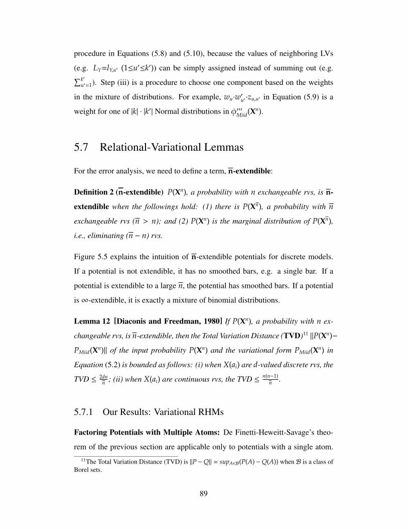
procedure in Equations (5.8) and (5.10), because the values of neighboring LVs

(e.g. LY=lY,u′ (1≤u′≤k′)) can be simply assigned instead of summing out (e.g.∑k′u′=1). Step (iii) is a procedure to choose one component based on the weights

in the mixture of distributions. For example, wu·w′u′ ·zu,u′ in Equation (5.9) is a

weight for one of |k| · |k′| Normal distributions in φ′′′Miid(Xn).

5.7 Relational-Variational Lemmas

For the error analysis, we need to define a term, n-extendible:

Definition 2 (n-extendible) P(Xn), a probability with n exchangeable rvs, is n-

extendible when the followings hold: (1) there is P(Xn), a probability with n

exchangeable rvs (n > n); and (2) P(Xn) is the marginal distribution of P(Xn),

i.e., eliminating (n − n) rvs.

Figure 5.5 explains the intuition of n-extendible potentials for discrete models.

If a potential is not extendible, it has no smoothed bars, e.g. a single bar. If a

potential is extendible to a large n, the potential has smoothed bars. If a potential

is∞-extendible, it is exactly a mixture of binomial distributions.

Lemma 12 [Diaconis and Freedman, 1980] If P(Xn), a probability with n ex-

changeable rvs, is n-extendible, then the Total Variation Distance (TVD)11‖P(Xn)−

PMiid(Xn)‖ of the input probability P(Xn) and the variational form PMiid(Xn) in

Equation (5.2) is bounded as follows: (i) when X(ai) are d-valued discrete rvs, the

TVD ≤ 2dnn ; (ii) when X(ai) are continuous rvs, the TVD ≤ n(n−1)

n .

5.7.1 Our Results: Variational RHMs

Factoring Potentials with Multiple Atoms: De Finetti-Heweitt-Savage’s theo-

rem of the previous section are applicable only to potentials with a single atom.

11The Total Variation Distance (TVD) is ‖P−Q‖ = supA∈B(P(A)−Q(A)) when B is a class ofBorel sets.

89

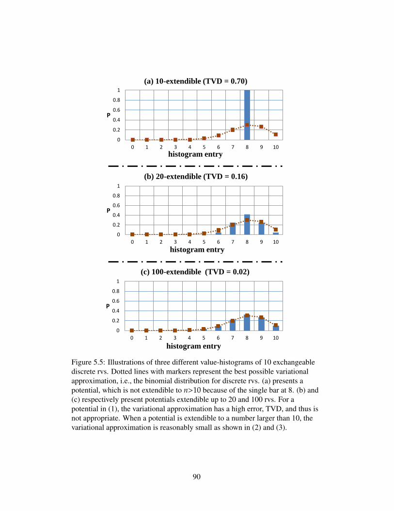
0

0.2

0.4

0.6

0.8

1

0 1 2 3 4 5 6 7 8 9 10

P

histogram entry

(a) 10-extendible (TVD = 0.70)

0

0.2

0.4

0.6

0.8

1

0 1 2 3 4 5 6 7 8 9 10

P

histogram entry

(b) 20-extendible (TVD = 0.16)

0

0.2

0.4

0.6

0.8

1

0 1 2 3 4 5 6 7 8 9 10

P

histogram entry

(c) 100-extendible (TVD = 0.02)

Figure 5.5: Illustrations of three different value-histograms of 10 exchangeablediscrete rvs. Dotted lines with markers represent the best possible variationalapproximation, i.e., the binomial distribution for discrete rvs. (a) presents apotential, which is not extendible to n>10 because of the single bar at 8. (b) and(c) respectively present potentials extendible up to 20 and 100 rvs. For apotential in (1), the variational approximation has a high error, TVD, and thus isnot appropriate. When a potential is extendible to a number larger than 10, thevariational approximation is reasonably small as shown in (2) and (3).

90

Here, we present our new theoretical result to construct variational models for

RHMs.

Lemma 13 [The Existence of a Variational Form] For P(Xn,Ym), a probability

with two atoms in an RHM, there are two new LVs, LX and LY, and a new potential

ΦXY(LX,LY) such that the following holds, limn,m→∞ P(Xn,Ym)

=

ˆΦ(LX,LY)

n∏i=1

φX(X(ai)|LX)m∏

j=1

φY(Y(b j)|LY) dLXLY

= PMiid(Xn,Ym).

Sketch of proof Assigning values to one atom (e.g. Ym = v) results in a new

potential with one atom, φ(Xn), which can be factored in Equation (5.2). It is not

hard to see that Φ(LX|v) is conditioned on v. Then, Φ(LX|Ym) can be factored into´Φ(LX,LY)

∏j φY(Y(b j)|LY)dLY.

To analyze variational error of potential with multiple atoms, we introduce a

new term (n,m)-extendible.

Definition 3 ((n,m)-extendible) P(Xn,Ym) is (n,m)-extendible when (1) there

is P(Xn,Ym), a probability with two sets of exchangeable rvs (n>n,m>m); and

(2) P(Xn,Ym) is the marginal distribution of P(Xn,Ym).

Lemma 14 (The Error of the Variational Parfactor) If P(Xn,Ym), a probabil-

ity with two exchangeable rvs in an RHM, is (n,m)-extendible, then the TVD

‖P(Xn,Ym)−PMiid(Xn,Ym)‖ is bounded as follows: (i) when Xn and Ym are re-

spectively dx-valued and dy-valued discrete rvs, the TVD ≤ 2dxnn +

2dymm ; (ii) when

Xn are dx-valued discrete and Ym are continuous, the TVD ≤ 2dxnn + m(m−1)

m ; (iii)

when Xn and Ym are continuous, the TVD ≤ n(n−1)n + m(m−1)

m .

Sketch of proof The intuition developed on the result in [Diaconis and Freed-

man, 1980] is that the error of a variational model is additive for an additional

atom.

91

0

0.2

0.4

0.6

0.8

1 2 4 8 16 32 64

10241286432168

k: the # of mixture components in the variational model Err

ors

of

Ap

pro

x.

(TV

D)

# of mixture components in the target probability

ktarget

k

32 64

1024 0.010 0.003

512 0.011 0.003

256 0.009 0.003

128 0.006 0.003

64 0.007 0.003

TVDs for k=32, k=64

Figure 5.6: The TVD of our variational models with k components. When k is areasonable size (e.g. 32), the TVD is very small even for a large number ofcomponents (e.g. 1024) in the target distributions.

It is straightforward to extend Lemma 14 for probability with more than two sets

of rvs, e.g. P(Xn,Ym,Zu).

Theorem 15 (The Error of a Variational RHM) Let Xg and XG is respectively

the set of all rvs in a parfactor g and an RHM G. Let P(Xg)(= 1zg

∏f∈gr(g) w f (X f ));

and P(XG)(= 1z

∏g∈G P(Xg)). The TVD ‖P(XG) − PMiid(XG)‖ is bounded by the

sum of TVD of each parfactor 1z

∑g∈G εg when εg is

∥∥∥P(Xg) − PMiid(Xg)∥∥∥.

Sketch of proof We can build a fully joint probability of all relational atoms with

the RHM. Then, Lemma 14 can be used to prove the TVD of the variational RHM.

5.8 Related Work

[Carbonetto et al., 2005] presents Nonparametric Bayesian Logic (NP-BLOG)

which is a variational representation for discrete variables using the Dirichlet Pro-

cess, a class of nonparametric methods for discrete variables. In principle, the

NP-BLOG and the variational RHMs have in common: compact representations

for exchangeable rvs. The difference is that NP-BLOG assumes that all discrete,

exchangeable rvs are ∞-extendible. Thus, it does not need error analysis or ap-

proximations for finite rvs. Here, we investigated further for several new direc-

tions: learning algorithms, continuous domains, and approximation errors. Our

error bounds for discrete variables provides the better understanding when using

92

NP-BLOG for a finite number of exchangeable rvs. For example, NP-BLOG has

at least the same error when approximating the potential (a) in Figure 5.5.

For discrete cases, exact methods, called value-histogram [de Salvo Braz et al.,

2005; Milch et al., 2008], represent potentials using histograms with only rel-

atively small (polynomial) numbers of entries. [Choi et al., 2011a] shows that

histogram representations for some special, aggregate, potentials can be approxi-

mately replaced by a fixed number of parameters. We generalize and expand the

concept to compress general-purpose histogram representations. In addition, we

clarify when the variational approximation is good to use and when not.

For continuous potentials, unfortunately, the histogram representation is not

applicable because it is not clear how to discretize continuous domains to build up

such histograms. Thus, most existing lifted inference for continuous models are

limited to Gaussian potentials [Choi et al., 2010a; 2011b; Ahmadi et al., 2011].

Thus, our representation is a unique lifted inference for non-Gaussian continuous

potentials.

[Singla and Domingos, 2008] presents the lifted Belief Propagation (BP) by

grouping discrete, exchangeable rvs, which send the same messages to neighbor-

ing rvs. The intuition, sending the same messages, assumes that the rvs are not

constrained among others, thus a single iid not but a mixture of iid rvs. Instead, our

lifted MCMC sends a distribution, has more expressive power, and may requires

fewer samples until the convergence. We believe that our variational models and

the lifted MCMC method can be a good complement to the lifted BP [Singla and

Domingos, 2008] for relational models.

When one mixture component of the variational form is given, one may think

about the Inversion Elimination [Poole, 2003], especially the Partial Inversion

Elimination [de Salvo Braz et al., 2006] because the mixture component is a prod-

uct of iid rvs. However, existing Inversion Eliminations has specific constraints,

and thus not directly applicable to the mixture of iid rvs. In this aspect, our varia-

tional models enable applying the Partial Inversion Elimination for lifted inference

by the variational learning.

93

Inferences in hybrid graphical models are proposed, e.g. [Lerner and Parr,

2001; Wang and Domingos, 2008]. [Lerner and Parr, 2001] presents an inference

algorithm for Linear-Gaussian Models where linear relations over rvs follow the

Gaussian distribution. [Wang and Domingos, 2008] proposed a MCMC algorithm

in Hybrid MLNs. However, it converts MLNs into a grounded, or propositional-

ized, one while sampling.

5.9 Experimental Results

We provide experimental results regarding the variational errors and the efficiency

and the accuracy of the LRVI in a real-world groundwater model.

First, we examine the error caused by k, the finite numbers of mixture com-

ponents. We assume that the target probabilities are ∞-extendible, so that the

TVD, variational error, can converge to 0 when k is large enough. P(X100) each

target probability over 100 exchangeable binary rvs is a mixture of binomials with

various k from 8 to 1024. For each target probability, our EM algorithm (Section

5.5) incrementally learn the variational model, k and φMiid with the EM algorithm.

Then, we measure the average TVD, variational error. Figure 5.6 shows the TVD

of our EM algorithm. It shows that the TVD becomes reasonably small (≤ 0.01)

with only 32 components even for target densities with 1024 components. When

we increase the number of rvs to 1000 P(X1000), the results are consistent. Thus,

the results show that the finite number of k is not an issues when the variational

approximation is applicable, i.e. n-extendible and n� n.

Second, we apply our variational learning algorithm to a real-world groundwa-

ter dataset, Figure 5.7 Republican River Compact Administration (RRCA) , which

is composed of measurements at over 10,000 wells and baseflow observations at

65 gages from 1918 until 2007.12 After calibration, the training dataset is a set of

partial continuous observations in a 480 (months) by 3420 (wells) matrix. First,

12Head predictions are available via the RRCA official website,http://www.republicanrivercompact.org.

94

(b)

Group A

Group B

Figure 5.7: Locations of clustered wells A and B in the RRCA dataset.

0

0.2

0.4

0.6

0.8

1

-5 -4 -3 -2 -1 0 1 2 3

cdf(A,1)cdf(A,2)cdf(A,3)cdf(A,4)cdf(B,1)cdf(B,2)cdf(B,3)

Group A

Group B F 𝑙𝐴,𝑢

(𝑥)

F 𝑙𝐵,𝑢′(𝑥)

Figure 5.8: Learned empirical distributions, Cdfs (FlA,u(x) and FlB,u′ (x)), of rvs ingroups A and B.

95

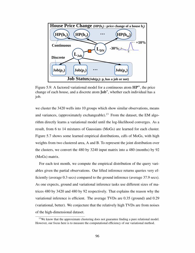
+10%

-30%

… HP(h1) HP(h2) HP(hm)

House Price Change (HP(hj) : price change of a house hj)

LDN

LJob

Job(p1) Job(p2) Job(pn) …

Job Status(Job(pi): pi has a job or not)

Discrete

Continuous

Figure 5.9: A factored variational model for a continuous atom HPm, the pricechange of each house, and a discrete atom Jobn, whether each individual has ajob.

we cluster the 3420 wells into 10 groups which show similar observations, means

and variances, (approximately exchangeable).13 From the dataset, the EM algo-

rithm directly learns a variational model until the log-likelihood converges. As a

result, from 6 to 14 mixtures of Gaussians (MoGs) are learned for each cluster.

Figure 5.7 shows some learned empirical distributions, cdfs of MoGs, with high

weights from two clustered area, A and B. To represent the joint distribution over

the clusters, we convert the 480 by 3240 input matrix into a 480 (months) by 92

(MoGs) matrix.

For each test month, we compute the empirical distribution of the query vari-

ables given the partial observations. Our lifted inference returns queries very ef-

ficiently (average 0.3 secs) compared to the ground inference (average 37.9 secs).

As one expects, ground and variational inference tasks use different sizes of ma-

trices 480 by 3420 and 480 by 92 respectively. That explains the reason why the

variational inference is efficient. The average TVDs are 0.35 (ground) and 0.29

(variational, better). We conjecture that the relatively high TVDs are from noises

of the high-dimensional dataset.

13We know that the approximate clustering does not guarantee finding a pure relational model.However, our focus here is to measure the computational efficiency of our variational method.

96

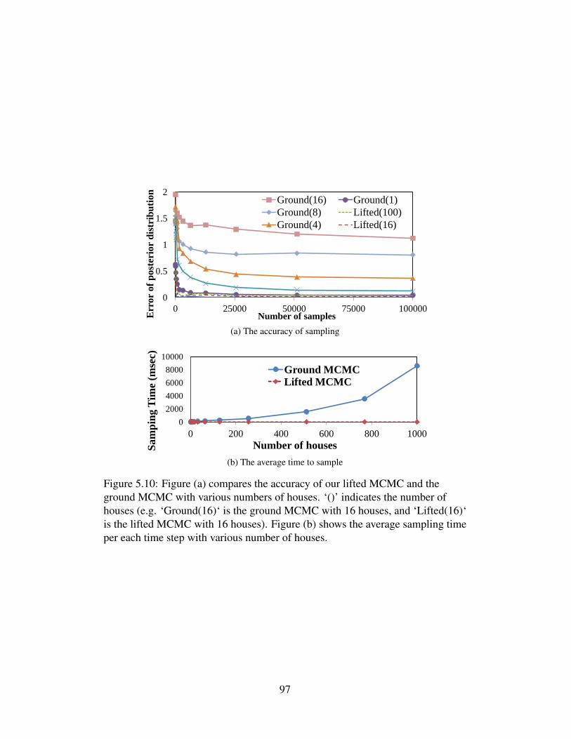
Err

or

of

po

ster

ior

dis

trib

uti

on

Number of samples

0

0.5

1

1.5

2

0 25000 50000 75000 100000

Ground(16) Ground(1)

Ground(8) Lifted(100)

Ground(4) Lifted(16)

(a) The accuracy of sampling

Sam

ping

Tim

e (m

sec)

Number of houses

0 2000 4000 6000 8000

10000

0 200 400 600 800 1000

Ground MCMC Lifted MCMC

(b) The average time to sample

Figure 5.10: Figure (a) compares the accuracy of our lifted MCMC and theground MCMC with various numbers of houses. ‘()’ indicates the number ofhouses (e.g. ‘Ground(16)‘ is the ground MCMC with 16 houses, and ‘Lifted(16)‘is the lifted MCMC with 16 houses). Figure (b) shows the average sampling timeper each time step with various number of houses.

97

Third, we compare the accuracy and the efficiency of our lifted MCMC algo-

rithm with a vanilla (ground) MCMC algorithm on an already factored variational

model. The model is composed of two relational atoms: a binary atom Jobn,

saying whether each individual has a job, and a continuous atom HPm, saying the

price change of each house. LJob is a latent variable, which represents the Bernoulli

parameters of φMiid(Jobn). LDN is a latent variable, which represents the mixture

of two Gaussians,14

φMiid(HPm) = LDN

m∏j=1

fN (HP(h j);−0.3, σ2DN)+(1−LDN)

m∏j=1

fN (HP(h j); 0.1, σ2UP).

Then, the potential between two latent variables follows a linear Gaussian:

Φ(LJob,LDN)=N(LJob−LDN, σ2JH).

Figure 5.10 (a) shows the accuracy of the two algorithms given the same number

of samples. That is, it measure the ratio of error to estimate a probability of a

randomly chosen variable x, |ptrue(x)−pMCMC(x)|/ptrue(x). It shows that our lifted

MCMC converges to the true density much faster than the ground MCMC. Figure

5.10 (b) shows the average sampling time (per step) with different number of RVS

(e.g. the number of houses).

5.10 Conclusion and Future Work

We propose new lifted relational variational inference algorithms for relational

hybrid models. Our main contributions are two folds: (1) in theory, we show that

a relational model, which can represent large-scale systems, is accurately repre-

sented by a variational model; (2) our lifted algorithms are the first to solve infer-

14Because the target distribution is a mixture of two iid Gaussians, the lifted Belief Propaga-tion (BP) [Singla and Domingos, 2008] is not applicable without a modification. Although wecan modify it for continuous domain, the lifted BP assumes that each house sends the same mes-sage,i.e. price. Here, the messages between houses should be constrained among others. That is,the prices of some houses go down, and then prices of the other houses should go up.

98

ence problems without referring ground rvs for non-Gaussian continuous models.

Experiments show that our algorithm outperforms the existing possible methods

in a real-world problem.

There are some limitations of this work. First, for continuous potentials, the

variational learning may require extensive computations. Especially, when there

is no analytic solution, we may need (up to) O(exp(n)) samples. Unfortunately,

this is a hard problem in general. Finding variational forms for well-known dis-

tributions, such as logistic regression [Doucet et al., 2000], would be interesting

future research. Second, clustering continuous exchangeable rvs is still unsolved

problem because of the noise in continuous data. We only know solutions for dis-

crete domains [Kok and Domingos, 2008; 2009]. However, the methods are not

directly applicable to continuous domains due to the noise.

99

CHAPTER 6

SUMMARY AND FUTURE WORK

This thesis presents efficient methods to answer questions on large-scale prob-

abilistic graphical models, specifically Relational Hybrid Models (RHMs). The

key contributions of this thesis are two folds: (1) novel lifted inference algorithms

for large-scale probabilistic graphical models with continuous variables (Chapter

2 and 3); and (2) new insights that transform probabilistic first-order languages

into compact approximations which allow efficient ways of inference (Chapter 4

and 5).

6.1 Summary of Contributions

This thesis offers the following contributions:

• It introduces new lifted inference algorithms that compute conditional and

marginal probabilities of probabilistic graphical models with continuous

variables, Relational Continuous Models (RCMs), especially the pairwise

linear Gaussian (Chapter 2) [Choi et al., 2010a];

• It presents a new exact Kalman filter (KF), the Lifted Relational Kalman

filter (LRKF), that enables scaling the exact Kalman filter from thousands

of variables to billions of variables (Chapter 3) [Choi et al., 2011b];

• It shows that typically used aggregate operators over Probabilistic Rela-

tional Graphical Models (PRGMs) and the existential quantification over

probabilistic first-order logic can be accurately approximated by linear con-

straints in Gaussian distributions. (Chapter 4) [Choi et al., 2011a];

100

• It proves that Relational Hybrid Models, relational models with continuous

and discrete domains, can be accurately approximated by variational mod-

els, composed of mixtures of independent and identically distributed(i.i.d.)

random variables. The approximation allows efficient inference procedures

on the large-scale probabilistic graphical models with hybrid domains (Chap-

ter 5) [Choi and Amir, 2011; 2012].

Chapter 2 introduces new lifted inference algorithms that compute conditional

and marginal probabilities of RCMs, large probabilistic graphical models with

continuous variables only. The algorithm is a key advance in exact inference for

RCMs, since most previous works are restricted to discrete domains. Given a

query and a set of observations, the algorithm exactly computes the conditional

probability of the query, when potentials satisfy specified conditions in the chap-

ter. The algorithm maintains relational structures during the inference procedure

for relational pair-wise potentials such as pairwise linear Gaussian potentials.

The Kalman filter (KF) is a computational tool with widespread applications

in robotics, financial and weather forecasting, environmental engineering and de-

fense. Given observation and state transition models, the KF recursively estimates

the state variables of a dynamic system. Chapter 3 presents a new efficient filtering

algorithm, the LRKF, for large-scale linear dynamic systems. The LRKF extends

the RCMs with pairwise linear Gaussian potentials in Chapter 2, and represents

dynamic systems in a relational (first-order) way. In each time step, the lifted

inference algorithm efficiently updates the large number of random variables at

the first-order (relational) level. The LRKF maintains compact pairwise relation-

ships among random variables even with individual observations. Thus, individual

attributes do not degenerate the relational structures into propositional ones. The-

oretical analysis and empirical tests show that this approach leads to significant

gains in efficiency and enables filtering for systems with very large numbers of

random variables.

101

Processing aggregate parfactors efficiently is a fundamental problem since they

involve functions commonly used in writing models. Chapter 4 adds efficient

exact methods for the binary case k=2, as well as efficient approximations for

the cases in which sets of aggregated variables are large, which is precisely the

situation in which we are more likely to use aggregate factors in the first place. The

chapter shows that aggregate operators over relational models can be accurately

approximated by linear constraints over Gaussian distributions. Thus, in many

case, calculating the conditional probability does not depend on the number of

random variables. The accuracy of approximation is close to optimal when the

model has a large number of random variables. The approximation will therefore

be an important part of practical applications of relational graphical models.

Finally, Chapter 5 presents new understandings that relate RHMs and varia-

tional models. The contributions of this chapter are two folds: (1) in theory, it

shows that a relational model, that can represent large-scale systems, is accurately

represented by a variational model; (2) the lifted variational inference algorithms

are the first to solve inference problems without referring to ground random vari-

ables for non-Gaussian continuous models. The variational models also represent

the discrete and continuous variables in a coherent way. RHMs are general, so that

the new insights can be applied to other models such as Markov Logic Networks

(MLNs) and Latent Tree Models (LTMs). Experiments show that the algorithm

outperforms the existing methods in a real-world problem.

6.2 Future Work

Most Relational Models assume that each set of random variables has the same

types of relationships with other sets. Thus, whenever an individual attribute is

assigned or observed to a random variable, the random variable is separated from

the relational structure. This thesis shows that it is possible to maintain relational

structures even if individual attributes are made to large linear dynamic systems

102

with continuous variable (Chapter 3) and to large-scale graphical models with both

discrete and continuous domains by approximations (Chapter 5). However, in dis-

crete models or non-Gaussian models, individual attributes prevent exact lifted in-

ference algorithms from maintaining relational structures. Thus, handling individ-

ual attributes for Relational Models with discrete domains would be a promising

research direction.

Another key challenge is to learn RPGMs from noisy data. Building a relational

model by clustering continuous random variables is hard especially for noisy con-

tinuous inputs. Suppose that a house X is on the border of two cities A and B.

A random variable representing the price of the house X would have similar rela-

tionships with random variables for housing prices both in A and random variable

in B. It is not clear that a random variable should be included either one cluster or

another. In this reason, solutions for discrete domains [Kok and Domingos, 2008;

2009] are not directly applicable to continuous models. One possible solution is

building several Relational Models with different granularities [de Salvo Braz et

al., 2009; Kiddon and Domingos, 2011]. Finding more principles to cluster con-

tinuous random variables may pave the way for new applications, such in econo-

metrics, computer vision, robot planning, and environmental engineering.

One limitation of the LRKF is that it shatters the model when the random vari-

ables in a relational atom receive different numbers of observations because their

variances and covariances become different. Approximate re-grouping of random

variables would be a general recourse in this case. Although the Gaussian distri-

bution has widespread use in real-world applications, the linearity assumption in

the KF limits the use of the Relational Kalman filter to non-linear dynamic sys-

tems. Thus, understanding principles for non-linear dynamic systems would be

crucial to building a new relational Extended Kalman filter (EKF). In the general

case, building a relational stochastic filter, e.g. Particle filter [Doucet et al., 2000],

could be an attractive alternative.

103

REFERENCES

[Ahmadi et al., 2011] Babak Ahmadi, Kristian Kersting, and Scott Sanner. Multi-evidence lifted message passing, with application to pagerank and the kalmanfilter. In Walsh [2011], pages 1152–1158.

[Apsel and Brafman, 2011] Udi Apsel and Ronen I. Brafman. Extended lifted in-ference with joint formulas. In Proceedings of the Twenty-Seventh Conferenceon Uncertainty in Artificial Intelligence, UAI 2011, pages 11–18, 2011.

[Bacchus, 1990] Fahiem Bacchus. Representing and reasoning with probabilisticknowledge: a logical approach to probabilities. MIT Press, Cambridge, MA,USA, 1990.

[Bahmani-Oskooee and Brown, 2004] Mohsen Bahmani-Oskooee and FordBrown. Kalman filter approach to estimate the demand for internationalreserves. Applied Economics, 36(15):1655–1668, 2004.

[Boutilier, 2009] Craig Boutilier, editor. IJCAI 2009, Proceedings of the 21stInternational Joint Conference on Artificial Intelligence, Pasadena, California,USA, July 11-17, 2009. IJCAI, 2009.

[Burgard and Roth, 2011] Wolfram Burgard and Dan Roth, editors. Proceedingsof the Twenty-Fifth AAAI Conference on Artificial Intelligence, AAAI 2011, SanFrancisco, California, USA, August 7-11, 2011. AAAI Press, 2011.

[Burgers et al., 1998] Gerrit Burgers, Peter Jan van Leeuwen, Geir Evensen, Ger-rit Burgers, and Gerrit Burgers. On the analysis scheme in the ensemble kalmanfilter. Monthly Weather Review, 126:1719–1724, 1998.

[Carbonetto et al., 2005] Peter Carbonetto, Jacek Kisynski, Nando de Freitas,and David Poole. Nonparametric bayesian logic. In Fahiem Bacchus andTommi Jaakkola, editors, Proceedings of the 21st Conference in Uncertaintyin Artificial Intelligence, UAI 2005, pages 85–93. AUAI Press, 2005.

[Choi and Amir, 2007] Jaesik Choi and Eyal Amir. Factor-guided motion plan-ning for a robot arm. In 2007 IEEE/RSJ International Conference on IntelligentRobots and Systems, IROS 2007, pages 27–32. IEEE, 2007.

104

[Choi and Amir, 2009] Jaesik Choi and Eyal Amir. Combining planning and mo-tion planning. In 2009 IEEE International Conference on Robotics and Au-tomation, ICRA 2009, pages 238–244. IEEE, 2009.

[Choi and Amir, 2011] Jaesik Choi and Eyal Amir. Lifted variational inference.Computer science research and tech reports, University of Illinois, 2011.

[Choi and Amir, 2012] Jaesik Choi and Eyal Amir. Lifted relational variationalinference. In Submitted for publication, 2012.

[Choi et al., 2008] Jaesik Choi, Won J. Jeon, and Sang-Chul Lee. Spatio-temporal pyramid matching for sports videos. In Michael S. Lew, Alberto DelBimbo, and Erwin M. Bakker, editors, Multimedia Information Retrieval, MIR2008, pages 291–297. ACM, 2008.

[Choi et al., 2010a] Jaesik Choi, Eyal Amir, and David Hill. Lifted inference forrelational continuous models. In Peter Grunwald and Peter Spirtes, editors,Proceedings of the Twenty-Sixth Conference on Uncertainty in Artificial Intel-ligence, UAI 2010, pages 126–134. AUAI Press, 2010.

[Choi et al., 2010b] Jaesik Choi, Jay Pujara, Vishwanth Tumkur Ramarao, andKe Wei. Identifying ip addresses for spammers. U.S. Patent No. 7,849,146,2010.

[Choi et al., 2011a] Jaesik Choi, Rodrigo de Salvo Braz, and Hung H. Bui. Effi-cient methods for lifted inference with aggregate factors. In Burgard and Roth[2011].

[Choi et al., 2011b] Jaesik Choi, Abner Guzman-Rivera, and Eyal Amir. Liftedrelational kalman filtering. In Walsh [2011], pages 2092–2099.

[Choi et al., 2011c] Jaesik Choi, Ke Wei, and Vishwanath Tumkur Ramarao. Fil-ter for blocking image-based spam. U.S. Patent No. 8,055,078, 2011.

[Choi et al., 2011d] Myung Jin Choi, Vincent Y. F. Tan, Animashree Anandku-mar, and Alan S. Willsky. Learning latent tree graphical models. Journal ofMachine Learning Research, 12:1771–1812, 2011.

[Chu et al., 2006] Wei Chu, Vikas Sindhwani, Zoubin Ghahramani, andS. Sathiya Keerthi. Relational learning with gaussian processes. In Bern-hard Scholkopf, John C. Platt, and Thomas Hoffman, editors, Proceedings ofthe Twentieth Annual Conference on Neural Information Processing Systems,NIPS 2006, pages 289–296. MIT Press, 2006.

[Cowell, 1998] Robert Cowell. Advanced inference in bayesian networks. InMichel I. Jordan, editor, Learning in graphical models, pages 27–49. MITPress, Cambridge, MA, 1998.

105

[Damien and Walker, 2001] Paul Damien and Stephen G Walker. Sampling trun-cated normal, beta, and gamma densities. Journal of Computational andGraphical Statistics, 10(2):206–215, 2001.

[Dasgupta, 1999] Sanjoy Dasgupta. Learning mixtures of gaussians. In The 40thAnnual Symposium on Foundations of Computer Science, FOCS 1999, pages634–644. IEEE Computer Society, 1999.

[de Finetti, 1931] B. de Finetti. Funzione caratteristica di un fenomeno aleatorio.Mathematice e Naturale, 1931.

[de Salvo Braz et al., 2005] Rodrigo de Salvo Braz, Eyal Amir, and Dan Roth.Lifted first-order probabilistic inference. In Kaelbling and Saffiotti [2005],pages 1319–1325.

[de Salvo Braz et al., 2006] Rodrigo de Salvo Braz, Eyal Amir, and Dan Roth.Mpe and partial inversion in lifted probabilistic variable elimination. In Pro-ceedings of the Twenty-First National Conference on Artificial Intelligence andthe Eighteenth Innovative Applications of Artificial Intelligence Conference,AAAI/IAAI 2006, pages 1123–1130. AAAI Press, 2006.

[de Salvo Braz et al., 2007] R. de Salvo Braz, E. Amir, and D. Roth. Lifted first-order probabilistic inference. In L. Getoor and B. Taskar, editors, An Introduc-tion to Statistical Relational Learning, pages 433–451. MIT Press, 2007.

[de Salvo Braz et al., 2009] R. de Salvo Braz, S. Natarajan, H. Bui, J. Shavlik,and S. Russell. Anytime lifted belief propagation. In Statistical RelationalLearning Workshop, 2009.

[Diaconis and Freedman, 1980] P. Diaconis and D. Freedman. Finite exchange-able sequences. Annals of Probability, 8(1):115–130, 1980.

[Diaconis, 1977] P. Diaconis. Finite forms of de finetti’s theorem on exchange-ability. Synthese, 36(2):271–281, 1977.

[Dıez and Galan, 2003] F. J. Dıez and S. F. Galan. Efficient computation for thenoisy MAX. International Journal of Approximate Reasoning, 18:165–177,2003.

[Doucet et al., 2000] Arnaud Doucet, Nando de Freitas, Kevin P. Murphy, andStuart J. Russell. Rao-blackwellised particle filtering for dynamic bayesiannetworks. In Craig Boutilier and Moises Goldszmidt, editors, Proceedings ofthe 16th Conference in Uncertainty in Artificial Intelligence, UAI 2000, pages176–183. Morgan Kaufmann, 2000.

[Esseen, 1942] Carl-Gustav Esseen. On the liapunoff limit of error in the the-ory of probability. Arkiv foer Matematik, Astronomi, och Fysik, A28(9):1–19,1942.

106

[Evensen, 1994] Geir Evensen. Sequential data assimilation with a nonlinearquasi-geostrophic model using monte carlo methods to forecast error statistics.Journal of Geophysical Research, 99:10143–10162, 1994.

[Fox and Gomes, 2008] Dieter Fox and Carla P. Gomes, editors. Proceedingsof the Twenty-Third AAAI Conference on Artificial Intelligence, AAAI 2008,Chicago, Illinois, USA, July 13-17, 2008. AAAI Press, 2008.

[Friedman et al., 1999] Nir Friedman, Lise Getoor, Daphne Koller, and Avi Pfef-fer. Learning probabilistic relational models. In Thomas Dean, editor, Proceed-ings of the Sixteenth International Joint Conference on Artificial Intelligence,IJCAI 1999, pages 1300–1309. Morgan Kaufmann, 1999.

[Getoor and Taskar, 2007] Lise Getoor and Ben Taskar. Introduction to StatisticalRelational Learning (Adaptive Computation and Machine Learning). The MITPress, 2007.

[Geweke, 1991] John Geweke. Efficient simulation from the multivariate normaland student-t distributions subject to linear constraints and the evaluation ofconstraint probabilities. In Proceedings the 23rd Symposium on the Interfacebetween Computer Sciences and Statistics, pages 571–578, 1991.

[Gottlob and Walsh, 2003] Georg Gottlob and Toby Walsh, editors. IJCAI 2003,Proceedings of the Eighteenth International Joint Conference on Artificial In-telligence, Acapulco, Mexico, August 9-15, 2003. Morgan Kaufmann, 2003.

[Gotze, 1991] F. Gotze. On the rate of convergence in the multivariate clt. TheAnnals of Probability, 19(2):724–739, 1991.

[Hajishirzi et al., 2009] Hannaneh Hajishirzi, Afsaneh Shirazi, Jaesik Choi, andEyal Amir. Greedy algorithms for sequential sensing decisions. In Boutilier[2009], pages 1908–1915.

[Halpern, 1990] Joseph Y. Halpern. An analysis of first-order logics of probabil-ity. Artif. Intell., 46(3):311–350, 1990.

[Hewitt and Savage, 1955] E. Hewitt and L.J. Savage. Symmetric measures oncartesian products. Trans. Amer. Math. Soc., 80:470–501, 1955.

[Hill et al., 2009] David J. Hill, Barbara S. Minsker, and Eyal Amir. Real-timebayesian anomaly detection in streaming environmental data. Water ResourcesResearch, 45:W00D28, 2009.

[Jha et al., 2010] Abhay Kumar Jha, Vibhav Gogate, Alexandra Meliou, and DanSuciu. Lifted inference seen from the other side : The tractable features. InJohn D. Lafferty, Christopher K. I. Williams, John Shawe-Taylor, Richard S.Zemel, and Aron Culotta, editors, Proceedings of the 24th Annual Conferenceon Neural Information Processing Systems, NIPS 2010, pages 973–981. CurranAssociates, Inc., 2010.

107

[John and Langley, 1995] George H. John and Pat Langley. Estimating continu-ous distributions in bayesian classifiers. In Philippe Besnard and Steve Hanks,editors, Proceedings of the Eleventh Annual Conference on Uncertainty in Ar-tificial Intelligence, UAI 1995, pages 338–345. Morgan Kaufmann, 1995.

[Kaelbling and Saffiotti, 2005] Leslie Pack Kaelbling and Alessandro Saffiotti,editors. IJCAI 2005, Proceedings of the Nineteenth International Joint Con-ference on Artificial Intelligence, Edinburgh, Scotland, UK, July 30-August 5,2005. Professional Book Center, 2005.

[Kalman, 1960] Rudolph Emil Kalman. A new approach to linear filtering andprediction problems. Transactions of the ASME–Journal of Basic Engineering,82(Series D):35–45, 1960.

[Kersting et al., 2006] K. Kersting, L. De Raedt, and T. Raiko. Logical hiddenmarkov models. Journal of Artificial Intelligence Research, 25:425–456, 2006.

[Kiddon and Domingos, 2011] Chloe Kiddon and Pedro Domingos. Coarse-to-fine inference and learning for first-order probabilistic models. In Burgard andRoth [2011].

[Kisynski and Poole, 2009] Jacek Kisynski and David Poole. Lifted aggregationin directed first-order probabilistic models. In Boutilier [2009], pages 1922–1929.

[Kok and Domingos, 2008] Stanley Kok and Pedro Domingos. Extracting se-mantic networks from text via relational clustering. In Walter Daelemans, BartGoethals, and Katharina Morik, editors, Machine Learning and KnowledgeDiscovery in Databases, European Conference, ECML/PKDD 2008, volume5211 of Lecture Notes in Computer Science, pages 624–639. Springer, 2008.

[Kok and Domingos, 2009] Stanley Kok and Pedro Domingos. Learning markovlogic network structure via hypergraph lifting. In Andrea Pohoreckyj Danyluk,Leon Bottou, and Michael L. Littman, editors, Proceedings of the 26th AnnualInternational Conference on Machine Learning, ICML 2009, volume 382 ofACM International Conference Proceeding Series, page 64. ACM, 2009.

[Koller and Pfeffer, 1997] Daphne Koller and Avi Pfeffer. Object-orientedbayesian networks. In Dan Geiger and Prakash P. Shenoy, editors, Proceed-ings of the Thirteenth Conference on Uncertainty in Artificial Intelligence, UAI1997, pages 302–313. Morgan Kaufmann, 1997.

[Kotz et al., 2000] S. Kotz, N Balakrishnan, and N.L. Johnson. Continuous Mul-tivariate Distributions. Wiley, New York, 2000.

[Lerner and Parr, 2001] Uri Lerner and Ronald Parr. Inference in hybrid net-works: Theoretical limits and practical algorithms. In Jack S. Breese andDaphne Koller, editors, Proceedings of the 17th Conference in Uncertainty inArtificial Intelligence, UAI 2001, pages 310–318. Morgan Kaufmann, 2001.

108

[Limketkai et al., 2005] Benson Limketkai, Lin Liao, and Dieter Fox. Relationalobject maps for mobile robots. In Kaelbling and Saffiotti [2005], pages 1471–1476.

[Mihalkova and Mooney, 2009] Lilyana Mihalkova and Raymond J. Mooney.Transfer learning from minimal target data by mapping across relational do-mains. In Boutilier [2009], pages 1163–1168.

[Milch and Russell, 2006] Brian Milch and Stuart J. Russell. First-order proba-bilistic languages: Into the unknown. In Stephen Muggleton, Ramon P. Otero,and Alireza Tamaddoni-Nezhad, editors, Inductive Logic Programming, 16thInternational Conference, ILP 2006, volume 4455 of Lecture Notes in Com-puter Science, pages 10–24. Springer, 2006.

[Milch et al., 2005] Brian Milch, Bhaskara Marthi, Stuart J. Russell, David Son-tag, Daniel L. Ong, and Andrey Kolobov. Blog: Probabilistic models withunknown objects. In Kaelbling and Saffiotti [2005], pages 1352–1359.

[Milch et al., 2008] Brian Milch, Luke S. Zettlemoyer, Kristian Kersting,Michael Haimes, and Leslie Pack Kaelbling. Lifted probabilistic inferencewith counting formulas. In Fox and Gomes [2008], pages 1062–1068.

[Ng and Subrahmanian, 1992] Raymond Ng and V. S. Subrahmanian. Probabilis-tic logic programming. Information and Computation, 101(2):150–201, 1992.

[Niemira and Saaty, 2004] Michael P. Niemira and Thomas L. Saaty. An analyticnetwork process model for financial-crisis forecasting. International Journalof Forecasting, 20(4):573–587, 2004.

[Paskin, 2003] Mark A. Paskin. Thin junction tree filters for simultaneous local-ization and mapping. In Gottlob and Walsh [2003], pages 1157–1166.

[Pfeffer et al., 1999] Avi Pfeffer, Daphne Koller, Brian Milch, and Ken T.Takusagawa. Spook: A system for probabilistic object-oriented knowledgerepresentation. In Kathryn B. Laskey and Henri Prade, editors, Proceedings ofthe Fifteenth Conference on Uncertainty in Artificial Intelligence, UAI 1999,pages 541–550. Morgan Kaufmann, 1999.

[Poole, 2003] David Poole. First-order probabilistic inference. In Gottlob andWalsh [2003], pages 985–991.

[Rasmussen and Ghahramani, 2001] Carl Edward Rasmussen and ZoubinGhahramani. Infinite mixtures of gaussian process experts. In Thomas G.Dietterich, Suzanna Becker, and Zoubin Ghahramani, editors, Advances inNeural Information Processing Systems 14, Neural Information ProcessingSystems: Natural and Synthetic, pages 881–888. MIT Press, 2001.

109

[Rice, 2006] John A. Rice. Mathematical Statistics and Data Analysis. DuxburyPress, 2006.

[Richardson and Domingos, 2006] Matthew Richardson and Pedro Domingos.Markov logic networks. Machine Learning, 62(1-2):107–136, 2006.

[Roweis and Ghahramani, 1999] Sam Roweis and Zoubin Ghahramani. A uni-fying review of linear gaussian models. Neural Computation, 11(2):305–345,1999.

[Rue and Held, 2005] H. Rue and L. Held. Gaussian Markov random fields: The-ory and applications. Springer, New York, 2005.

[Shenoy, 2006] Prakash P. Shenoy. Inference in hybrid bayesian networks usingmixtures of gaussians. In Rina Dechter and Thomas Richardson, editors, Pro-ceedings of the 22nd Conference in Uncertainty in Artificial Intelligence, UAI2006. AUAI Press, 2006.

[Singla and Domingos, 2007] Parag Singla and Pedro Domingos. Markov logicin infinite domains. In Ronald Parr and Linda C. van der Gaag, editors, Pro-ceedings of the Twenty-Third Conference on Uncertainty in Artificial Intelli-gence, UAI 2007, pages 368–375. AUAI Press, 2007.

[Singla and Domingos, 2008] Parag Singla and Pedro Domingos. Lifted first-order belief propagation. In Fox and Gomes [2008], pages 1094–1099.

[Sorenson and Stubberud, 1968] H. W. Sorenson and A. R. Stubberud. Non-linear filtering by approximation of the a posteriori density. International Jour-nal of Control, 8:33–51, 1968.

[Walsh, 2011] Toby Walsh, editor. IJCAI 2011, Proceedings of the 22nd Interna-tional Joint Conference on Artificial Intelligence, Barcelona, Catalonia, Spain,July 16-22, 2011. IJCAI/AAAI, 2011.

[Wang and Domingos, 2008] Jue Wang and Pedro Domingos. Hybrid markovlogic networks. In Fox and Gomes [2008], pages 1106–1111.

[Xu and Jordan, 1995] Lei Xu and Michael I. Jordan. On convergence propertiesof the em algorithm for gaussian mixtures. Neural Computation, 8:129–151,1995.

[Xu et al., 2009] Zhao Xu, Kristian Kersting, and Volker Tresp. Multi-relationallearning with gaussian processes. In Boutilier [2009], pages 1309–1314.

[Xu et al., 2012] Tiangfang Xu, Albert J. Valocchi, Jaesik Choi, and Eyal Amir.Improving groundwater flow model prediction using complementary data-driven models. In XIX International Conference on Computational Methodsin Water Resources, CMWR 2012, 2012.

110

[Zhang, 2002] Nevin Lianwen Zhang. Hierarchical latent class models for clusteranalysis. In Rina Dechter and Richard S. Sutton, editors, Proceedings of theEighteenth National Conference on Artificial Intelligence and Fourteenth Con-ference on Innovative Applications of Artificial Intelligence, AAAI/IAAI 2002,pages 230–237. AAAI Press / The MIT Press, 2002.

111