Embed Size (px)
Citation preview

Balogh András
REAL-TIME VISUALIZATION OF DETAILED TERRAIN
Budapesti Műszaki- és Gazdaságtudományi Egyetem Villamosmérnöki és Informatikai Kar
Automatizálási és Alkalmazott Informatika Tanszék
KONZULENS
Rajacsics Tamás BUDAPEST, 2003

2
HALLGATÓI NYILATKOZAT
Alulírott Balogh András, szigorló hallgató kijelentem, hogy ezt a diplomatervet meg
nem engedett segítség nélkül, saját magam készítettem, csak a megadott forrásokat
(szakirodalom, eszközök, stb.) használtam fel. Minden olyan részt, melyet szó szerint,
vagy azonos értelemben de átfogalmazva más forrásból átvettem, egyértelműen, a forrás
megadásával megjelöltem.
Tudomásul veszem, hogy az elkészült diplomatervben található eredményeket a
Budapesti Műszaki- és Gazdaságtudományi Egyetem, a feladatot kiíró egyetemi
intézmény saját céljaira felhasználhatja.
Kelt: Budapest, 2003. 05. 16.
.....................................................................Balogh András

3
Összefoglaló
A nagy kiterjedésű, részletdús felületek valósidejű megjelenítése a számítógépes
grafika egyik alapvető problémája. A téma fontosságát az is mutatja, hogy a hosszú
évek óta tartó folyamatos kutatások eredményeképpen mára számtalan algoritmus látott
napvilágot. Azonban az egyre növekvő követelmények újabb módszerek kifejlesztését
igénylik. Munkámban megoldást keresek a domborzat felbontásának futásidejű
növelésére procedúrális geometria hozzáadásával. Természetesen az ilyen procedúrális
részlet valósidejű beillesztése a domborzatba nem egyszerű feladat. A legtöbb
algoritmus az előfeldolgozási feltételei miatt egyáltalán nem képes az ilyen típusú
felületek megjelenítésére.
Dolgozatomban először röviden elemzem, és összehasonlítom az eddig
kifejlesztett legsikeresebb terepmegjelenítő algoritmusokat, rámutatok azok előnyeire és
korlátaira egyaránt, majd az egyik legújabb és leghatékonyabb algoritmust alapul véve
kifejlesztek egy olyan módszert, ami alkalmassá teszi tetszőleges felbontású,
procedúrális geometriával dúsított domborzatok valósidejű megjelenítésére.
Mindemellett bemutatok egy olyan árnyalási technikát is, ami a legmodernebb grafikus
hardverek tudását maximálisan kihasználva lehetővé teszi az ilyen részletes
domborzatok valósághű, pixel pontos megvilágítását is.

4
Abstract
This thesis focuses on real-time displaying of large scale, detail rich terrains.
Although terrain rendering algorithms have been studied for a long time, it is still a very
active field in computer graphics. The growing requirements and changing conditions
always call for new solutions. In this work I explore possible methods to increase the
perceived resolution of the surface by adding extra procedural detail to the terrain
geometry at run-time. This is not an easy task, as it can be seen by the lack of available
algorithms supporting it. High performace terrain rendering techniques all depend on
special precomputed data for a fixed size, static terrain, which makes them unable to
deal with such detailed surfaces generated at run-time.
I start out with describing and comparing several well known algorithms, that
take different approaches to terrain visualization. Then, based on one of these
algorithms, I introduce a novel method to extend the algorithm to support real-time
visualization of high resolution terrain surfaces with extra detail geometry. To
complement the geometry with a decent lighting solution, I also develop a robust
technique to perform accurate per pixel shading of such a detailed terrain, using the
latest crop of graphics hardware.

5
Table of Contents
1 Introduction.................................................................................................................. 7
1.1 Overview................................................................................................................. 7
1.2 Computer graphics .................................................................................................. 8
2 Modelling the terrain................................................................................................. 10
2.1 Geometrical description of the surface ................................................................. 10
2.2 Using heightmaps and displacement maps ........................................................... 11
2.3 Surface normal and tangent plane......................................................................... 11
3 Displaying the geometry............................................................................................ 14
3.1 Overview............................................................................................................... 14
3.2 Introducing Level of Detail................................................................................... 15
3.3 View-dependent refinement.................................................................................. 17
3.4 Data management ................................................................................................. 18
4 A survey of algorithms .............................................................................................. 19
4.1 Overview............................................................................................................... 19
4.2 Chunked LOD....................................................................................................... 20
4.3 Progressive meshes ............................................................................................... 21
4.4 The ROAM algorithm........................................................................................... 23
4.5 The SOAR algorithm ............................................................................................ 25
4.6 Miscellaneous issues............................................................................................. 30
4.6.1 Geomorphing ................................................................................................. 30
4.6.2 Occlusion culling ........................................................................................... 30
4.6.3 Z fighting ....................................................................................................... 31
4.6.4 Multi-frame amortized mesh building ........................................................... 32
5 Improving the SOAR algorithm............................................................................... 33
5.1 More efficient refinement ..................................................................................... 33
5.2 Lazy view-frustum culling.................................................................................... 39
6 Extending SOAR with detail geometry.................................................................... 41
6.1 Overview............................................................................................................... 41
6.2 Basic concepts....................................................................................................... 42
6.3 Detailed explanation ............................................................................................. 42

6
7 Terrain lighting .......................................................................................................... 46
7.1 Overview............................................................................................................... 46
7.2 Lighting basics ...................................................................................................... 48
7.3 Per pixel dynamic lighting of detailed surfaces.................................................... 51
8 Implementation .......................................................................................................... 55
8.1 Overview............................................................................................................... 55
8.2 The framework...................................................................................................... 56
8.3 The preprocessing module .................................................................................... 56
8.4 The rendering module ........................................................................................... 57
8.5 Testing environment and performance ................................................................. 58
9 Summary..................................................................................................................... 60
10 References................................................................................................................. 61
Appendix A: Glossary .................................................................................................. 62
Appendix B: Color plates ............................................................................................. 63

7
1 Introduction
1.1 Overview
One of the most important use case of computers is simulation. It allows us to do
things that would not be possible (or would be too dangerous, or just too expensive)
otherways. Simulation is a very wide concept. Whether we are simulating the collision
of entire galaxies, or some tiny particles in a cyclotron, or the efficiency and behaviour
of a jet engine under various circumstances, or the view from an airplane 10’000 feet
above, it is all the same. Simulation mimics reality1. Thus, we call the result Virtual
Reality (VR), where everything seems and works like in reality, except that it is not
real2. A VR system has lots of components, the one responsible for creating audiovisual
stimuli is one of the most important ones, since humans can comprehend this kind of
information the most. Here we will be concerned exlusively with the visualization part.
More specifically the visualization of large scale, detailed terrain surfaces.
Applications ranging from aerial and land traffic training and control software,
to entertaining computer games, all require detailed, consistent views of massive terrain
surfaces. There are a lot of issues involved in terrain visualization. Most important ones
are the compact, yet accurate representation of the terrain model (describing its
geometry, material properties and such), efficient management (i.e. paging from mass
storage devices) of this dataset, and displaying the geometry extracted from this model,
so that the result is comparable to what one would see in reality.
We must not forget that simulation is always an approximation. Even if we
make some very exact and precise calculations, we do them with regards to a model. A
simplified model of the part of the real world we are interested in. It is very important to
have a firm grasp on these concepts, because it is essential when one has to make
important decisions and balance tradeoffs during engineering some kind of simulation
application.
1 Or, perhaps, unreality. One could simulate an imagined world, where one could bend the rules
of physics. 2 Well, what is real, and what is not is really a question of philosophy. According to Platon, one
cannot talk about things that do not exist.

8
1.2 Computer graphics
Computer Graphics (CG for short) is in itself a very diverse field. There are a
number of very good textbooks on the topic [11][12] and I very much recommend
reading at least one of them to get familiar with the concepts. Although I will do my
best to make this paper easy to understand for everyone, I will still assume some basic
knowledge in the field of computer graphics.
There are some very different methods for photorealistic versus non-
photorealistic (like an illustration), and real-time versus off-line rendering. The main
goal is of course to display some kind of image on the screen. Even this simple task of
displaying an already calculated image has its problems. Today’s computer displays
have severe limitations, most importantly that they lack the dynamic range of the human
eye. We could (and should) use higher internal precision for our calculations (this is
called HDR (High Dynamic Range) rendering) to achieve more realistic reflections and
other effects (like the specular bloom), but we still should not forget that ultimately it
will be displayed on a device with reduced dynamic range. That is a limitation we have
to live with1. There are some image processing methods, like adaptive contrast
enhancement, that tries to bring detail into the compressed dynamic range to make the
image more enjoyable, but it is really just cheating the eye by distorting the source
range. This technique is mainly used as a post processing operation on commercials or
movies. It is too expensive for real-time visualization, however.
There are many ways to display a scene in computer graphics. What is common
is that for each pixel on the screen, we have to determine a color value that represents
the incoming light from that direction. The difference is how the light contributions are
calculated for each pixel. Global illumination methods, like radiosity and raytracing are
physically most accurate, but they are very expensive in terms of required calculations.
Since we are aiming at real-time visualization, they are not appropriate for our purposes.
Incremental image synthesis on the other hand uses a local illumination model, meaning
that each object is displayed as a set of primitives (points, lines or triangles) and each
primitive is shaded independently of other parts of the scene. Thus it is possible to build
special, heavily pipelined hardware accelerators capable to process geometry and
fragments (pixel data) at an incredible speed, but this comes at a price. Shadows, and
1 Some military flight simulators utilize special display devices that are capable of displaying
very bright spots (simulating mainly ground lights), but they are expensive and still limited to points.

9
inter-object reflections that are handled elegantly by the global lighting solutions, have
to be added using various tricks and hacks. Although these tricks are not always
perfectly accurate, they do not have to be. In our case it is enough to give the user an
illusion of reality. Also, some techniques from raytracing and radiosity can be used
directly in the local lighting solution. Eventually it turns out that near raytraced quality
images can be rendered in real-time using cheap, consumer level hardware accelelrators.
In the rest of this document we will be concerned solely with using hardware
accelerated rendering techniques for real-time visualization of large-scale detailed
terrains.
10
2 Modelling the terrain
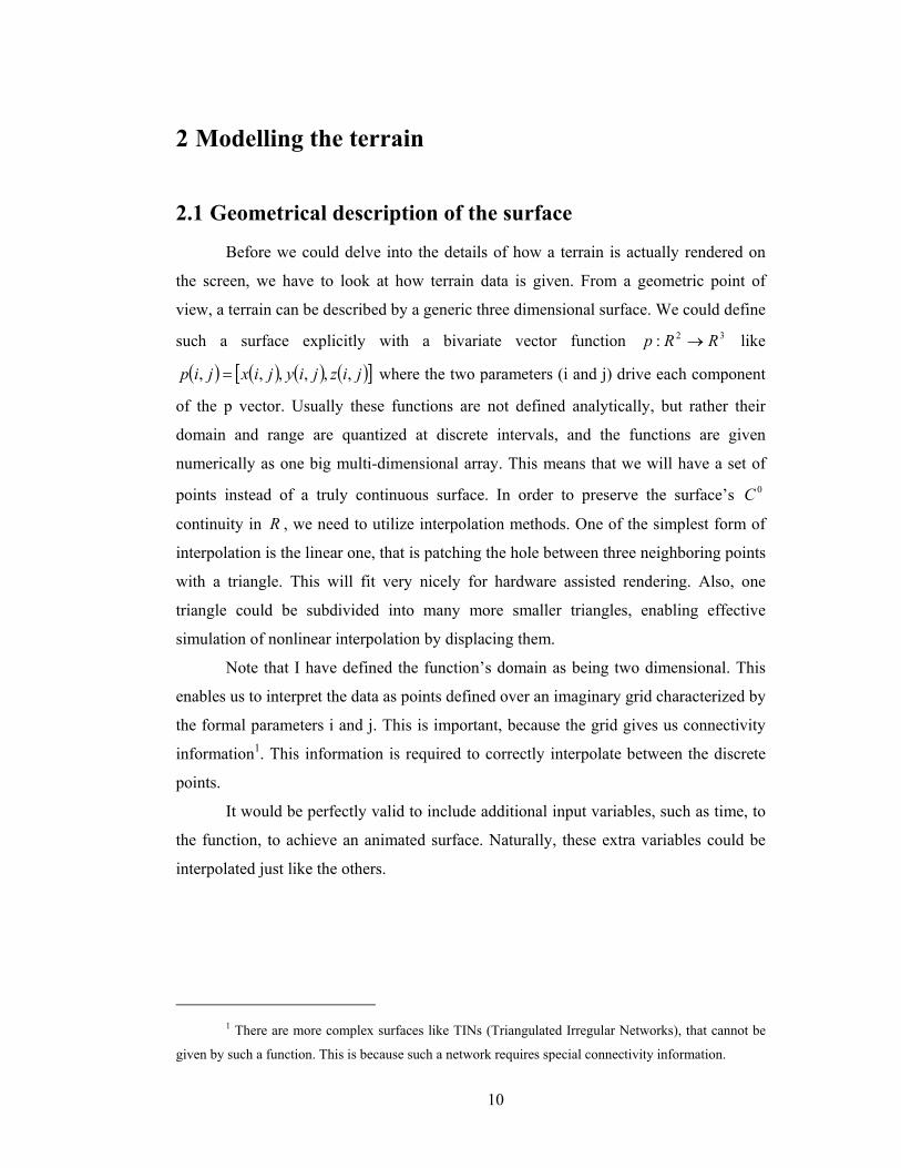
2.1 Geometrical description of the surface
Before we could delve into the details of how a terrain is actually rendered on
the screen, we have to look at how terrain data is given. From a geometric point of
view, a terrain can be described by a generic three dimensional surface. We could define
such a surface explicitly with a bivariate vector function 32: RRp → like
( ) ( ) ( ) ( )[ ]jizjiyjixjip ,,,,,, = where the two parameters (i and j) drive each component
of the p vector. Usually these functions are not defined analytically, but rather their
domain and range are quantized at discrete intervals, and the functions are given
numerically as one big multi-dimensional array. This means that we will have a set of
points instead of a truly continuous surface. In order to preserve the surface’s 0C
continuity in R , we need to utilize interpolation methods. One of the simplest form of
interpolation is the linear one, that is patching the hole between three neighboring points
with a triangle. This will fit very nicely for hardware assisted rendering. Also, one
triangle could be subdivided into many more smaller triangles, enabling effective
simulation of nonlinear interpolation by displacing them.
Note that I have defined the function’s domain as being two dimensional. This
enables us to interpret the data as points defined over an imaginary grid characterized by
the formal parameters i and j. This is important, because the grid gives us connectivity
information1. This information is required to correctly interpolate between the discrete
points.
It would be perfectly valid to include additional input variables, such as time, to
the function, to achieve an animated surface. Naturally, these extra variables could be
interpolated just like the others.
1 There are more complex surfaces like TINs (Triangulated Irregular Networks), that cannot be
given by such a function. This is because such a network requires special connectivity information.

11
2.2 Using heightmaps and displacement maps
Despite the fact that the function described in the previous section gives us the
most flexibility when defining a surface, in most cases though, terrain is not given as
such a generic surface, but as simple elevation data, called a heightmap. This could be
described with a simpler 32: RRp → function, like
( ) ( )[ ]zzxyxzxp ,,,, = . It is easy to see that this is a
special case of the original function. This formula is
much more constrained than the previous one, since
overhanging surfaces (like the one shown in Figure 2-1)
cannot be modelled with it. Still this format is preferred
over the generic one, because it is much more efficient in
terms of memory usage, since all we need to store is a simple scalar for each point (the
other two components are implicitly given by the function definition). Since on most
systems usually data throughput is the bottleneck, this is a major win. Generalizing this
idea means that we could use a simple vector function that describes the base form of
the surface, and then use another compact scalar function that changes the base surface.
A very nice example for adding more detail to a surface in such a way is called
displacement mapping. Displacement mapping is a technique that displaces each point
on the surface in the direction of the normal vector (n) by an amount given by a
bivariate scalar function RRd →2: . So the final, displaced position is
( ) ( ) ( ) ( )jidjinjipjir ,,,, += . Note that the heightmap is really a displacement map
defined over a plane. Next generation hardware accelerators will have built-in support
for mesh subdivision and displacement, making this technique ideal for adding detail to
a smooth surface.
Obviously, if the surfaces are given numerically rather than analytically then
function interpolation must be used to combine surfaces with different resolutions. Later
in this paper (in Chapter 6) I will also use a special kind of surface combining technique
to add more detail to a base surface.
2.3 Surface normal and tangent plane
A vector that is perpendicular to the surface at a given point is called a normal.
The surface normal has lots of uses. Some of the more important ones are collision
detection and response, and lighting calculations. Actually, we are not really interested
Figure 2-1 Overhangs

12
in the normal vector itself, but the tangent plane defined by it. It might help to think
about the normal, as the representation of
the plane. To be exact, the normal vector
defines only the facing direction of the
plane, not its position, but for most
computations that is enough. By defining a
point on the plane, we can also pin down
the plane’s exact location. Note that there
are an infinite number of normal vector and
point combinations that define the same
plane. The normal could be scaled by an
arbitrary positive1 scalar, and any other
point on the plane is a good candidate for
the plane definition. Most of our
calculations require the normal to be unit length, however, making the vector unique to
the plane. Such unit length vectors are said to be normalized. We can normalize any
vector by dividing each of its components by the length of the vector. Having the unit
normal and a point on the plane, we can calculate the distance of any point from the
plane as illustrated on Figure 2-2.
When using homogeneous coordinates, we can express a plane in a much more
compact and convenient way. Instead of defining a unit normal vector and a point
separately, we can describe the plane with a simple four component vector q, where the
first three components represent the facing direction of the plane and the fourth
component is the negated distance of the plane from the
origo. Using this vector, we can calculate any point’s
distance from the plane by calculating the dot product
between the point and the plane (see equations on the
left). The distance is signed, meaning that the plane
divides the space into a positive and a negative half space. Moreover, we can use the
same dot product operation to calculate the sine of the angle between the plane and a
unit length direction vector.
1 Negating the vector will still define the plane with the same set of points but it will have a
different facing direction.
[ ][ ][ ]( )
[ ]npnnnqqrnpnrprnd
rrrrr
nnnn
ppppp
zyx
wzyx
zyx
wzyx
−==−=−=
=
=
=
0
Figure 2-2 Calculating the distance between
a point and a plane .

13
Now, that we know how to use the tangent plane, let us see, how to find it for a
given point on a surface. For each point on the parametric surface, there is exactly one
tangent plane, that can be defined by the contact point and the normal vector of the
surface at that point. Using the function from the previous section, the normal vector is
defined as follows1:
jp
ipn
∂∂
×∂∂
=
The partial derivatives of the surface lay on the tangent plane, and the cross
product is perpendicular to both tangent vectors. Thus the resulting vector is also
perpendicular to the tangent plane. Even if the surface is not given analytically, we can
still compute an approximation using finite differencing. Note that this formula does not
usually result in a unit length normal vector, so we must take care of normalizing it, if
necessary. Even if we can skip normalizing, calculating the direction of the normal
vector on-the-fly for every point is still a costly operation. So it is recommended to
calculate and store them beforehand, if possible. Also, when the surface is given
analitically then the normal vectors can also be derived analitically, which might be
cheap enough to be evaluated runtime.
1 Note that the definition is the same for both left and right handed coordinate systems. The
results will be different, because the cross product operator is defined differently in the two coordinate
systems.

14
3 Displaying the geometry
3.1 Overview
Assuming we know everything about the surface geometry, displaying it seems
like an easy task.. Note that we are not interested in the material properties of the
terrain, nor in the characteristics of the environment (like lightsources) for the moment.
These topics will be discussed later (in Chapter 7). Right now we are only concerned
with pure geometry. Now, all we have to do is walk the surface grid, and build a
triangle mesh by connecting neighbouring vertices. Unfortunately this method is not
usable in real-time visualizaton. Suppose we have to display a terrain that has an area of
a million hectares (100Km * 100Km) at 10cm resolution. In this case we would have to
display a triangle mesh consisting of no less than a thousand milliard ( 1210 ) vertices.
Since for each vertex we need at least a couple of bytes for height information (and in
the generic case for two more coordinates), we would have to deal with terrabytes of
data. Even if we had the memory and the bandwidth necessary to access all these data,
we would still not be able to process this much information in real time.
For interactive display, we need to render an image at minimum 15 fps (frames
per second). For the illusion of continuous animation at least 24 fps is required1, but 60-
80 fps is much more plausible to the human brain. Today’s state of the art workstations
are capable of processing about a 100 million vertices per second. This means that if we
are to achieve an enjoyable framerate, we have to live with 4 million vertices per frame.
Note that these are theoretical peak rates. In practice this means a lot less, about 200
thousand triangles per frame. Of course these are just raw numbers, real performance
depends on the complexity of the vertex and fragment programs used, the number of
state changes required (which causes expensive pipeline stalling), the number of pixels
rendered (depth complexity), and so on...
1 Movie films are played back at 24fps, but sometimes it’s rather unconvincing (e.g. when the
camera is turning around in a small room, the motion feels jerky).

15
3.2 Introducing Level of Detail
As we can see, the brute force method proposed in the previous section is not
going to suffice. We have to find a way to display that huge dataset by accessing and
using a limited number of vertices. This inevitably means that we have to drop detail.
Of course it is up to the application to decide how much detail should be dropped, and
where. The ultimate goal is to drop as much unnecessary detail as possible while still
preserving a good level of perceived image quality. In general, these kinds of algorithms
are collectively called LOD (Level of Detail) algorithms.
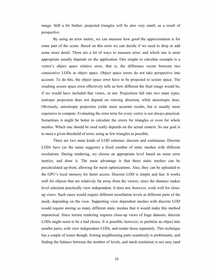
Looking at Figure 3-1 immediately demonstrates the problems caused by the
lack of LOD. Every triangle on the screen have approximately the same size in world
space. The nearby regions (which make up the majority of the pixels on the screen) are
made up of only a couple of triangles, clearly missing every kind of detail. A little
farther away, there is a sudden density change (thick black), where the terrain surface is
almost parallel to the viewing plane (i.e. the surface normal is perpendicular to the
viewing vector, as is the case with silhouette edges), thus triangles there will be very
small when projected to screen space and so have a minimal contribution to the final
Figure 3-1 A wireframe rendering of a terrain without LOD
16
image. Still a bit farther, projected triangles will be also very small, as a result of
perspective.
By using an error metric, we can measure how good the approximation is for
some part of the scene. Based on this error we can decide if we need to drop or add
some more detail. There are a lot of ways to measure error, and which one is most
appropriate usually depends on the application. One simple to calculate example is a
vertex’s object space relative error, that is, the difference vector between two
consecutive LODs in object space. Object space errors do not take perspective into
account. To do this, the object space error have to be projected to screen space. The
resulting screen space error effectively tells us how different the final image would be,
if we would have included that vertex, or not. Projections fall into two main types:
isotropic projection does not depend on viewing direction, while anisotropic does.
Obviously, anisotropic projection yields more accurate results, but is usually more
expensive to compute. Evaluating the error term for every vertex is not always practical.
Sometimes it might be better to calculate the errors for triangles or even for whole
meshes. Which one should be used really depends on the actual context. So our goal is
to meet a given threshold of error, using as few triangles as possible.
There are two main kinds of LOD schemes: discrete and continuous. Discrete
LODs have (as the name suggests) a fixed number of static meshes with different
resolutions. During rendering, we choose an appropriate level based on some error
metrics, and draw it. The main advantage is that these static meshes can be
precalculated up-front, allowing for mesh optimizations. Also, they can be uploaded to
the GPU’s local memory for faster access. Discrete LOD is simple and fast. It works
well for objects that are relatively far away from the viewer, since the distance makes
level selection practically view independent. It does not, however, work well for close-
up views. Such cases would require different tessellation levels at different parts of the
mesh, depending on the view. Supporting view dependent meshes with discrete LOD
would require storing so many different static meshes that it would make this method
impractical. Since terrain rendering requires close-up views of huge datasets, discrete
LODs might seem to be a bad choice. It is possible, however, to partition an object into
smaller parts, with view independent LODs, and render those separately. This technique
has a couple of issues though. Joining neighbouring parts seamlessly is problematic, and
finding the balance between the number of levels, and mesh resolution is not easy (and

17
is probably very application specific). Although discrete LOD schemes are quite rigid,
we will see some examples of efficient terrain rendering methods that use discrete LOD.
On the contrary, continuous LOD (also called CLOD) schemes offer a vast
(practically unlimited) number of different meshes, without requiring additional storage
space for each of them. These algorithms assemble the approximating mesh at runtime,
giving the application much finer control over mesh approximation. This means that
these methods require less triangles to achieve the same image quality. The downside is
that these CLOD algorithms are usually quite complex, the cost of building and
maintaining the mesh is high. Also, since the mesh is dynamic, it must reside in system
memory and sent over to the GPU every frame1. Most terrain rendering algorithms
(including the one my work is based upon) are based on CLOD schemes, because it is
more flexible and scalable then discrete LOD.
3.3 View-dependent refinement
For continuous level of detail we need algorithms that construct a triangle mesh
that approximates the terrain as it would be seen from a particular location. In our case
this means that only vertices that are visible and play a significant role in forming the
shape of the terrain should be selected into the mesh. Finer tesselation occurs in nearby
terrain and at terrain features. These kind of algorithms use a so called view-dependent
refinement method. The result is a mesh that is more detailed in the areas of interest,
and less detailed everywhere else. Refinement methods can be grouped into two main
categories. The first one is bottom-up refinement (also called decimation), which starts
from the highest resolution mesh, and reduces its complexity, until an error metric is
met. The other one is called top-down refinement, which starts from a very low
resolution base mesh, and adds detail only where necessary. The bottom-up method
gives more optimal triangulations (that is, a better approximation, given the same
triangle budget), but the calculations required are proportional to the size of the input
data. The top-down method, on the other hand, while results in a slightly less optimal
triangulation, is insensitive to the size of the input data. Its calculation requirements
depend only on the size of the output mesh, which in our case is much lower than the
input. Legacy algorithms, like [3], were based on the bottom up method, because input
data was small, and rendering was expensive. Today almost every algorithm is based on
1 With fast AGP (Accelerated Graphics Port) bus, this is usually not a bottleneck.

18
the top-down scheme, since the size of input datasets have increased by some orders of
magnitude, while rendering performance is much higher (so rendering a couple of more
triangles than necessary will not hurt overall performance).
This is a perfect example of the precious balancing required when engineering
performance critical applications. One has to balance carefully, and make important
tradeoffs. With today’s hardware, it is cheaper to send a little more triangles than
spending long CPU cycles just to decide that a few of those triangles were unnecessary.
It is always very important to identify the bottleneck in the processing pipeline. It is safe
to say, that today’s GPUs (Graphic Processing Unit) can process as many vertices as it
is possible to send down the bus1. With time, bottlenecks move from one part of the
processing pipeline to another. Thus every so often these methods must be revisited and
evaluated.
It is also very important, that the resulting mesh is continuous, so it must not
have T-junctions (also called T-vertices), where cracks might appear. There are a
number of ways to avoid such cracks, but these depend on the exact algorithm used.
3.4 Data management
Of course with huge terrains there is still the problem of accessing the data. If
the surface data has to be paged in from an external storage device, it is called out-of-
core refinement. Mass storage devices usually have very poor random access
characteristics, but have an acceptable performance for linear data access. By reordering
the dataset in a way, that a more linear access pattern is used, we can achieve much
better performance. Also, spatial locality means better cache usage, and thus improves
overall performance. There are many ways to deal with this problem. In this paper I will
only briefly introduce the method used by the SOAR algorithm.
1 Assuming a standard transform stage setup.

19
4 A survey of algorithms
4.1 Overview
In the last decade there have been some very intense work in the field of terrain
rendering. Today, there exist a lot of different algorithms, each having its own strengths
and drawbacks. In this survey I am going to briefly describe some of the more
successful ideas. They will also serve as a reference, so my work can be compared
against previous results.
Most algorithms described here render terrains described by heightfields. These
heightfields are usually defined over a square grid (if it is not square, then a tight
bounding square could be used instead). One of the
most straightforward method for partitioning such a
grid into smaller parts is by means of a quadtree. A
quadtree is a datastructure, where each node has four
children. When used in terrain rendering, the root
node represents the whole surface, and the child
nodes subdivide the parent into four smaller
partitions, and so on. Figure 4-1 shows quadtree
partitioning. Some early terrain rendering techniques
use this spatial partitioning only to perform fast
gross culling against the viewing frustum. In this case the algorithm always have to
subdivide to the lowest level for rendering, but large blocks can be culled away easily if
outside the frustum. It is very easy to add some LOD to this method by subdividing
deeper in branches with a higher error. Of course this kind of subdivision does not
guarantee that the resulting mesh will be free of T-junctions. The mesh will likely to
have cracks where different level of detail parts connect. The restricted quadtree
triangulation (RQT) can solve this problem. Such a restricted triangulation can be
ensured by walking in a dependency graph defined over a grid (see [6] for example),
and adding the necessary extra vertices. Figure 4-2 illustrates this method:
Figure 4-1 Quadtree hierarchy

20
Figure 4-2 Walking the dependency graph, and adding extra vertices where necessary results in a
restricted quadtree triangulation (Illustration by Renato Pajarola).
There are a couple of issues with this technique, though. This explicit
dependency walk is quite expensive, especially when dealing with lots of vertices. Also,
it only adds vertices, not triangles, and it is not trivial how to build a new triangulation
for the resulting set of vertices. Now that we have seen a basic approach and its
problems, let us investigate some more sophisticated techniques.
4.2 Chunked LOD
Thatcher Ulrich’s work [7] is a relatively simple, yet very effective terrain
rendering technique based on discrete level of detail. Contrary to other, more
complicated algorithms, its aim is not to achieve an optimal triangulation, but to
maximize triangle throughput, while minimizing CPU usage. As it has been discussed
in the previous chapter, it builds on the fact, that today’s graphics subsystems are so
fast, that it is usually cheaper to render a bit more triangles than to spend a lot of CPU
cycles to drop some of the unnecessary ones. Of course, level of detail management is
still required, but at a much coarser level. So the idea is to apply view dependent LOD
management not to single vertices, but to bigger chunks of geometry.
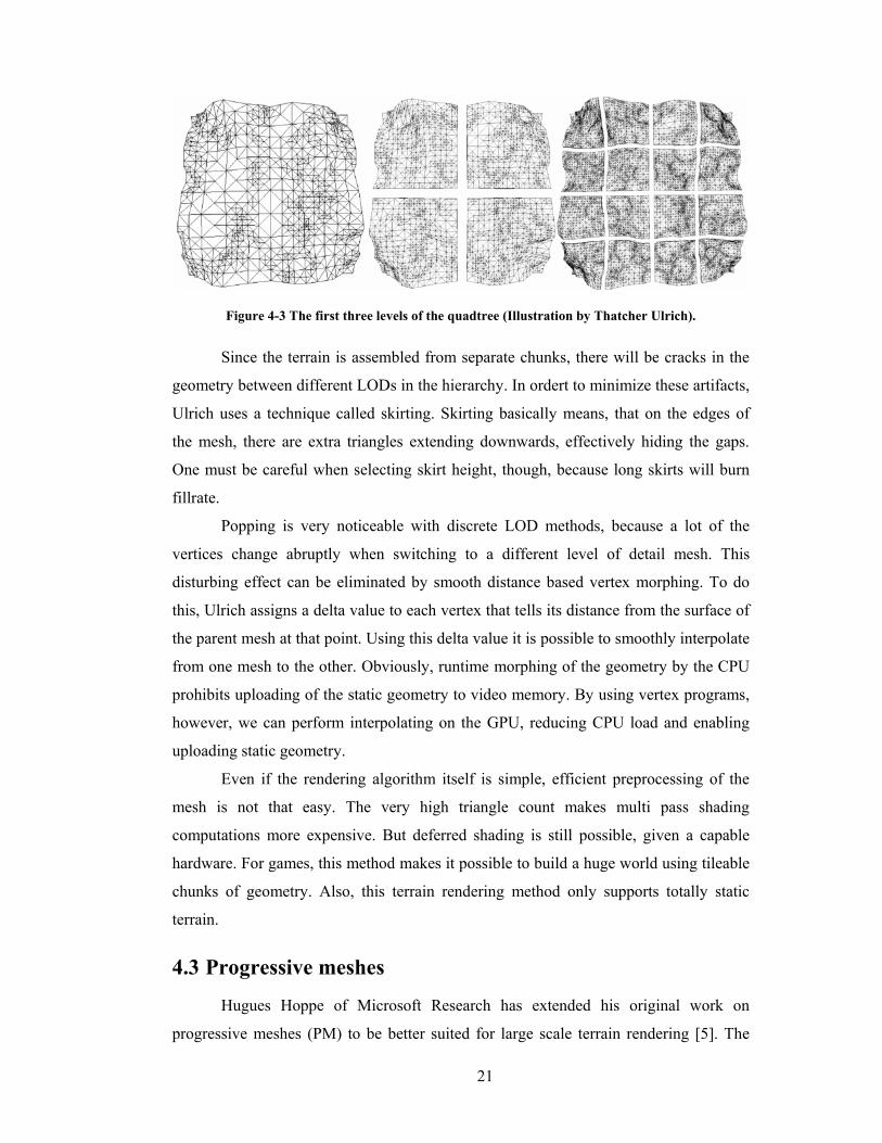
As a preprocessing step, a quadtree of terrain chunks is built (see Figure 4-3).
Every node is assigned a chunk, not just the leaves. Each chunk can contain an arbitrary
mesh, enabling very effective mesh optimization in the preprocessing step. The meshes
on different levels in the tree have different size in world space. The tree does not have
to be full, nor balanced, making adaptive detail possible. Each chunk is self contained
(the mesh and the texture maps are all packed together), making out-of-core data
management and rendering easy and efficient. During rendering the quadtree nodes are
culled against the viewing frustum as usual. The visible nodes are then split recursively,
until the chunk’s projected error falls below a threshold.
21
Figure 4-3 The first three levels of the quadtree (Illustration by Thatcher Ulrich).
Since the terrain is assembled from separate chunks, there will be cracks in the
geometry between different LODs in the hierarchy. In ordert to minimize these artifacts,
Ulrich uses a technique called skirting. Skirting basically means, that on the edges of
the mesh, there are extra triangles extending downwards, effectively hiding the gaps.
One must be careful when selecting skirt height, though, because long skirts will burn
fillrate.
Popping is very noticeable with discrete LOD methods, because a lot of the
vertices change abruptly when switching to a different level of detail mesh. This
disturbing effect can be eliminated by smooth distance based vertex morphing. To do
this, Ulrich assigns a delta value to each vertex that tells its distance from the surface of
the parent mesh at that point. Using this delta value it is possible to smoothly interpolate
from one mesh to the other. Obviously, runtime morphing of the geometry by the CPU
prohibits uploading of the static geometry to video memory. By using vertex programs,
however, we can perform interpolating on the GPU, reducing CPU load and enabling
uploading static geometry.
Even if the rendering algorithm itself is simple, efficient preprocessing of the
mesh is not that easy. The very high triangle count makes multi pass shading
computations more expensive. But deferred shading is still possible, given a capable
hardware. For games, this method makes it possible to build a huge world using tileable
chunks of geometry. Also, this terrain rendering method only supports totally static
terrain.
4.3 Progressive meshes
Hugues Hoppe of Microsoft Research has extended his original work on
progressive meshes (PM) to be better suited for large scale terrain rendering [5]. The

22
idea of progressive meshes is to build a special datastructure that allows rapid extraction
of different level of detail meshes that represent a good approximation of an arbitratry
triangle mesh. Also, this datastructure can handle not only geometry, but possibly other
attributes associated with each vertex or corner of the mesh (a corner is a vertex, face
pair), like material properties and such.
Building a good PM representation for the mesh is crucial. The process starts
with the original high resolution mesh, and then gradually reduces its complexity by
collapsing selected edges to a vertex. During this mesh decimation, we save collapse
information, making the process reversible. The result is a coarse base mesh, together
with a list of vertex split operations. The order of edge collapsing is very important to
form a good PM. There are a number of different algorithms for edge selection. For
view dependent refinement, the active front of vertices is visited, and a vertex split or an
edge collapse operation is performed based on the projected error. This PM
representation is very efficient for streaming data. First, only the coarse mesh is loaded,
and later, as we need more detail, we can load more vertex split data.
The preparation of the progressive mesh is computationally very expensive, and
as such, have to be done as a preprocessing step. Since the simplification procedure
should be performed bottom-up, it would prohibit processing of huge datasets that do
not fit into main memory at once. Hoppe introduces an alternative block based recursive
simplification process that permits simplificaton of large meshes. Hoppe also introduced
a couple of other enhancements over the original algorithm. He introduced smooth level
of detail control via geomorphing, and also redesigned the runtime datastructures to
have output sensitive memory requirements. Of course, these changes can be
generalized and used for arbitrary meshes also, not just for terrains.
The main advantage of using a progressive mesh is that it supports arbitrary
meshes. This means that PM geometry is not tied to a regular grid, and as a result,
usually a fraction of triangles (50-75%) are enough to approximate the original mesh,
compared to the other methods.
The downside of this method is that the runtime view dependent refinement
procedure is quite expensive. However, there is another method, called VIPM (View
Independent Progressive Meshes), that has the benefits of a good progressive mesh
representation, without the complicated computations required by the view dependent
refinement. For relatively small scale objects, VIPM is definitely a win, but for large
terrains it is hard to make it useful.

23
4.4 The ROAM algorithm
Mark Duchaineau et al. developed this remarkable algorithm mainly for
simulating low altitude flights. ROAM stands for Real-time Optimally Adapting
Meshes. Adapting meshes is a key concept in this algorithm. Since this algorithm has
been designed mainly for flight simulation purposes, it was a reasonable assumption to
make, that camera movement is continuous. Since there is no sudden change in the
viewpoint, it seems to be safe to exploit frame to frame coherence, and assume that the
mesh in the next frame will only differ in a few triangles. This means that there is no
need to regenerate the whole mesh from scratch every frame. It effectively allows the
algorithm to maintain a high resolution mesh (referred to as the active cut), and only
change it little by little every frame.
ROAM operates on a triangle bintree (a triangulation can be seen on Figure 4-4).
This structure allows for incremental refinement and decimation. To do this on-the-fly
mesh refinement, ROAM maintains two priority queues that drive the split and merge
operations. The queues are filled with triangles, sorted by their projected screen space
error. In every frame some triangles are split, bringing in more detail, and others are
merged into coarser triangles. Since the bintree is progressively refined, it is possible to
end the refinement at any time, enabling the application to maintain a stable framerate.
In order to avoid cracks (T-junctions) in the mesh, one has to recursively visit the
neighbours of the triangle and subdivide them if necessary (this is called a forced split,
see Figure 4-5). This is a quite expensive operation. Of course the fact that only a few
Figure 4-4 ROAM triangulation for an overhead view of the terrain
(Illustration by Mark Duchaineau).

24
triangles need updating would still justify this extra overhead, but ROAMs biggest flaw
turned out to be in this initial assumption.
For low resolution terrain the chain of dependecy to follow when fixing cracks is
not too deep. For higher resolution meshes this operation gets more expensive. Also, the
number of triangles that need updating
(splitting or merging) depends on the
relative speed of the camera. It is
important to note the term relative.
Camera speed should be measured
relative to terrain detail. Given the
same camera movement, the number of
triangles flown over (and thus, the
number of triangles need to be updated) depends on terrain resolution. If the relative
speed is high (and it will be, for high resolution terrain, no matter, how slow the camera
is moving), the number of triangles that pass by the camera will be high too. Also, since
most triangles in the approximating mesh consist of the nearby ones, it means that most
of the mesh will need updating.
So the bottom line is, that for highly detailed terrain, the approximating triangle
mesh will be so different every frame, that there is no point in updating the mesh from
last frame. It would mean dropping and then rebuilding most of the mesh every frame,
only to save the remaining couple of triangles. Considering how expensive these merge
and split operations are, it is clearly a bad idea to do incremental refinement. This is
worsened by the feedback loop effect. As one frame takes more time to render, during
that time the camera moves farther, requiring the next frame to change even more of the
mesh, that takes even more time to render, and so on.
This algorithm is a fine example for demonstrating how the bottleneck moves in
the processing pipeline, and how it affects performance. A couple of years ago this
algorithms seemed to be unbeatable (well, it is still very good for relatively low detail
terrains), but on today’s hardware it is very difficult to make it efficient. Lately there
has been some work to overcome this fundamental flaw in the algorithm, mainly by
working on chunks of triangles instead of individual triangles, but it is still not the right
solution.
Figure 4-5 Forced split to avoid T-junctions
(illustration by M. Duchaineou)

25
4.5 The SOAR algorithm
The SOAR (Stateless One-pass Adaptive Refinement) algorithm has been
developed by Peter Lindstrom and Valerio Pascucci at the Lawrence Livermore
National Laboratory. It combines the best methods published to date, and extends them
with some very good ideas. The result is a relatively simple, yet very powerful terrain
rendering framework. It has many independent components: an adaptive refinement
algorithm with optional frustum culling and on-the-fly triangle stripping, together with
smooth geomorphing based on projected error, and a specialized indexing scheme for
efficient paging of data required for out-of-core rendering. The heart of the method (as
its name, SOAR suggests) is the refinement procedure. Although the original paper
recommends some techniques for each component, all the other components can be
replaced or even left out alltogether. This makes it easy to compare various techniques
in the same framework. This also enables us to focus on one component of the
framework at a time. Since this algorithm serves as the basis to my work, I am going to
give a more in-depth description.
The refinement algorithm generates a new mesh from scratch every frame, thus
avoiding ROAMs biggest problem. The downside is that SOAR can not be interrupted
in the middle of the refinement. Once we started a new mesh, it is necessary to finish it
in order to get a continuous surface. In reality this is not a serious limitation, because it
is possible to adjust the error threshold between frames, so if one frame took too long to
build, the implementation could adaptively change refinement parameters.
Figure 4-6 Longest edge bisection
SOAR refinement is based on the longest edge bisection of isosceles right
triangles (see Figure 4-6). It subdivides each tirangle by its hypotenuse, creating two
smaller triangles. This subdivision scheme is quite popular amongst terrain renderers,

26
because it has two nice properties. First and most important is that it can be refined
locally, meaning that a small part of the mesh can be subdivided more than the other
parts, without breaking mesh continuity (of course, we have to follow some simple
constraints to ensure continuity, see later). This is essential for every CLOD algorithm.
Secondly, the new vertices introduced by each subdivision lay on a rectilinear grid,
making it easy to map a surface onto it.
The vertices are naturally categorized into levels, by the depth of the recursion.
The algorithm starts with the root vertex at level zero. Every vertex has four children
and two parents (vertices on the edge of the mesh have two children and one parent
only, and obviously, the root vertex has no parents at all). This hierarchy of vertices
could be represented as a DAG (Directed Acyclic Graph).
In practice, we almost always want to map our surface onto a square, not a
triangle. It is straightforward to build such a square by joining two triangles by their
hypotenouse, making a diamond, or joining four triangles by their right apex (illustrated
in Figure 4-7). We choose the latter one, for reasons discussed later. Now, the resulting
square base mesh can be recursively subdivided to any depth by the longest edge
bisection. Note that this kind of mesh has a somewhat constrained resolution. The
vertices introduced by this subdivision will always lay on a regular nn× grid, where
12 += kn . The number of levels in such a grid is kl 2= (so the number of levels is
always even). This might seem to be a serious limitation, but any surface could be
partitioned into such squares, and each partition could be rendered separately. Of course
one would have to take special care when joining such meshes to avoid cracks between
them.
It is also very important to note that this regular grid does not constrain the
layout of the output mesh. It only gives us a way to walk a hierarchy of vertices and
defines connectivity between them. So the input data for the refinement is not
constrained to heightfields. It can handle general 3D surfaces with overhangs as long as
the points of the surface can be indexed with two parameters (as it has been described in
Chapter 2.1).

27
Figure 4-7 Left: Joining four triangles forms a square. Middle: Refining triangles individually
results in cracks. Right: Crack prevention
Although the mesh can be refined locally, this subdivision scheme does not
automatically guarantee mesh continuity. In order to avoid T-junctions, we have to
follow a simple rule. Let us call the vertices that are in the resulting mesh active. For
each active vertex, all of its parents (and recursively all of its ancestors) must be active
too. This condition guarantees that there are no cracks in the mesh. This could be
ensured easily by visiting every vertex in the mesh and activating parents recursively
where necessary. As we have seen with previous algorithms, this dependency walk is a
very costly operation, and as such, should be avoided, if possible.
So how can we avoid these costly operations? Well, vertices are activated
(selected into the mesh) based on some kind of
projected error metrics. All we have to do is
ensure that these projected errors are nested, that
is, a vertex’s projected error must always be
smaller than any of its ancestors’. This way, if a
vertex is active then all of its ancestors will be
active, resulting in a continuous mesh. Now, the
question is, how to ensure these nesting
properties? Propagating the object space error
terms during preprocessing is not enough.
Consider a case when a child vertex is much
closer to the camera than its parent. Due to the
nature of the perspective projection, the projected error could be much higher for the
nearby vertex, even though its object space error is smaller. Since projection depends on
the relative position of the camera, it must be recalculated for each vertex, every frame,
making preprocessing impossible.
Figure 4-8 Bounding sphere
hierarchy (Illustration by P.
Lindstrom and V. Pascucci)

28
SOAR handles this problem in a very elegant and efficient way. It assigns
bounding spheres to vertices (Figure 4-8). These spheres must be nested, so that a
vertex’s bounding sphere contains all of its descendant vertices’ bounding spheres. This
nested hierarchy of bounding spheres can be built as a preprocessing step. Each sphere
can be described by a simple scalar value representing its radius. Now, if we project
every vertex’s object space error from the point on its bounding sphere’s surface that is
closest to the camera (Figure 4-9), then the resulting projected error will be nested, thus
cracks eliminated.
Of course this means that the projected error might be much higher than it really
is. This way more vertices will be selected into the mesh, than would be necessary for a
given error threshold. Considering that most of the extra vertices would be required for
crack prevention anyway, the added cost is not significant.
The nested sphere hierarchy also enables very efficient culling to the viewing
frustum. If a sphere is totally outside the frustum, then its vertex is culled, with all of its
descendants. This way big chunks of unseen geometry can be culled away early in the
processing pipeline. Note that this does not break the mesh continuity, since if a
vertex’s parent is culled then the vertex itself will also be culled. Also, if a sphere is
totally inside one plane, than all of its descendants will be inside, thus further checking
against that plane is unnecessary. By keeping a flag for the active planes, we can make
sure that only spheres intersecting at least one plane will be checked.
Now that we know how it is possible to decide if a given vertex is active, we can
continue our discussion about the refinement procedure. The main idea is pretty simple.
It recursively subdivides the four base triangles one by one, until the error threshold is
Figure 4-9 Error is projected from the nearest point on the bounding sphere.

29
met. The tricky part is building a continuous generalized triangle strip during refinement
(see Figure 4-10), that can then be passed to the hardware for rendering. Each triangle is
processed left to right. This means that first
we subdivide along its left child then
subdivide along the right child. In order to
make the strip continuous, we have to swap
triangle sides each level. So that the meaning
of “left” and “right” alternates between
consecutive levels of refinement. Since this
swapping also affects triangle winding,
sometimes degenerate triangles have to be
inserted into the strip. Otherwise a lot of the
triangles would turn up in the mesh
backfacing1. The refinement procedure keeps
track of swapping by using a parity flag. The new vertex’s parity flag is then compared
against the last vertex’s parity in the strip and a degenerate triangle is inserted if they are
equal. For a more detailed explanation refer to the original papers [1][2], or read
Chapter 5.1 where a more efficient refinement is discussed.
The framework also supports a nice method for smooth geomorphing of terrain
vertices, where the morphing starts from the interpolated vertex position and ends at the
real vertex position, and is driven by the vertex’s projected error. This is better than
time based geomorphing, since its stateless (no need to remember morphing vertices),
and vertices only morph when the camera is moving, making it practically undetectable.
Another very important component of the framework is the indexing scheme.
When dealing with huge datasets, the bottleneck will almost always be at the I/O
device. In these cases cache coherent data access can result in a drastical speedup. All
we have to do is store the surface vertices in an order that is close to the refinement
order. One such indexing scheme presented by the original paper is hierarchical
quadtree indexing. Although it is a little sparse (meaning that it requires more storage
space than traditional linear indexing), it does a great job when dealing with huge
1 Such triangles will be culled away by the graphics subsystem leaving a hole in the mesh. The
graphics subsystem could be configured not to clull backfacing triangles, but it is not a good idea to do so,
since it saves a lot of fillrate, and also makes z-fighting less likely to happen.
Figure 4-10 Single generalized triangle
strip for the whole mesh (Illustration by
P. Lindstrom and V. Pascucci).

30
external datasets1. The exact details of how to implement this indexing scheme (together
with some other alternatives) can be found in the original paper [2].
4.6 Miscellaneous issues
4.6.1 Geomorphing
Every time a new vertex is added to or removed from the mesh, the triangles
sharing that vertex will suddenly change (causing the infamous popping effect). Since
the human brain is very sensitive to changes, even a small number of popping can be
very disturbing. So it is important to totally eliminate these abrupt changes in vertex
positions. Although we can tell if a vertex suddenly jumps, we can not tell if a vertex is
at the correct position or not. Geomorphing techniques are based on this fact, tricking
our brains by slowly moving the new vertex to its real position. There are two main
kinds of geomorphing methods: time and error driven. As we have already seen when
describing the terrain rendering techniques, error based morphing is preferred, because
it morphs only during camera movement and does not need to remember the state (e.g.
time) for morphing vertices. Note that for per vertex lighting, not just the position, but
the normal vector also requires smooth morphing. The interpolation of the normal
vector results in the shifting of the triangle’s color, which might be noticeable. When
lighting is independent of the actual surface, then vertex morphing works without
problems.
Obviously, geomorphing only makes sense when dealing with big error
thresholds. If we render a mesh with projected errors below one pixel, than it is
unnecessary. Before implementing geomorphing, consider its computing overhead.
Sometimes it might be better to skip morphing, and just build a more accurate mesh
instead.
4.6.2 Occlusion culling
Another well known acceleration technique is occlusion culling. These
algorithms search for occluders in the scene (e.g. a nearby hill) and then cull every
detail occluded by it. These methods perform well with scenes having a considerable
1 Today’s CPUs are so much faster than memory modules that quadtree indexing results in a
considerable speedup even when the whole dataset fits in the computer’s main memory.

31
depth complexity. Problem is that every chain is as strong as its weakest link. In the
worst case we will look at the terrain from birds view, and there will be minimal
occlusion (haveing depth complexity of one). Since we require our rendering algorithm
to be fast enough in the worst case, there is no win in optimizing the best case. In this
case the oclusion culling algorithm will only give unnecessary overhead.
4.6.3 Z fighting
The ultimate goal of terrain rendering is to show the little features on the ground
in front of our feet and to show the distant mountains on the horizon. This means that
the 24bit Z-buffer found on most of today’s graphics cards is not going to suffice.
Because the insufficient precision, when rastering triangles in the distance, some pixels
will get the same depth value, disabling depth sorting. This phenomenon is known as Z-
fighting. Z-fighting can be reduced considerably by enabling backface culling. Backface
culling is a very cheap operation and it also reduces fillrate requirements, so it is worth
using. Unfortunatelly using this technique still cannot eliminate Z-fighting completely.
Also, there is another technique that might be useful, called depth clamping. When
depth clamping is enabled, the hardware does not perform clipping to the near and far
planes, instead it clamps the fragment’s depth value to the depth range. This means that
nearby objects will not be clipped, but they will get the same Z value, thus it might
result in some rendering artifacts (it is like rendering without a depth-buffer). It is still
better than clipping the triangle and usually enables us to push the near plane a little
farther without noticeable artifacts.
There are also other, more complicated methods, that increase depth precision,
like cutting up the viewing frustum to two or more parts, then rendering the terrain one
part a time, clearing the z-buffer between the parts. This method is not really
convenient, because it requires some difficult triangle surgery where the frustums
connect, to avoid cracks in the mesh.
As we can see, the best solution would be to use a 32bit z-buffer. Combined
with depth clamping, it would give all the precision a terrain renderer would probably
ever need. There are already some graphics cards supporting 32bit depth, and it is safe
to say that it will be a common feature in the near future.

32
4.6.4 Multi-frame amortized mesh building
When the mesh refinement operation is very expensive compared to the
rendering of the mesh (e.g. out-of-core rendering), it is common, to do these tasks in
separate threads. So, even if the refinement is only capable of building 10 meshes a
second, we could still display it at 60+ FPS, allowing for smooth camera movement. Of
course, refinement should work on another mesh. So this doubles the memory
requirements. This method assumes that camera movement is slow relative to terrain
detail. Otherways, swapping of the meshes will result in severe popping. Unfortunately,
this asynchronous refinement makes error based geomorphing practically useless. Even
though time based geomorphing might work, it would still be very difficult to make it
efficient. If the camera’s orientation is not restricted, then view frustum culling should
be turned off, so that the camera could turn around freely. Obviously, this means, that
we have to build and render a much bigger mesh, to meet the same error threshold.

33
5 Improving the SOAR algorithm
5.1 More efficient refinement
One of the most performance critical component of SOAR is the refinement
procedure that builds a single generalized triangle strip for the whole mesh in one pass.
The first paper [1] introduced a very simple, recursive algorithm for generating the
mesh. Although it is very short and easy to understand, it is rather inefficient. It suffers
from evaluating the same vertices (calculating its projected error, and performing view-
frustum culling) multiple times. In their second SOAR paper [2] the authors addressed
this issue and proposed a simple improvement over their previous algorithm, that avoids
some of these unnecessary calculations, by moving up the recursion by one level.
However, it turns out that there is still a lot of room for improvement. In this section I
am going to describe an alternative refinement algorithm that produces a more optimal
triangle strip and at the same time visits less inactive vertices.
In order to understand the main ideas behind the new mesh generation
algorithm, we have to investigate the
nature of triangle strips first. A triangle
strip is a special format for defining
adjoining triangles. Each new vertex is
assumed to form a triangle with the
previous two vertices. Defining the
primitives in such a format is very
efficient, because for n triangles, only n+2
vertices are required, compared to 3n for a
list of independent triangles. Also, the two
vertices borrowed from the previous
triangle do not have to be transformed and
lit again by the GPU1. Winding is automatically swapped after every vertex in order to
make all triangles face the same direction. When turning around corners, triangle
winding may get out of sync, flipping the faces of triangles. In order to avoid face
1 Note that using indexed primitives also solves most of these problems.
Figure 5-1 Triangle stripping

34
flipping, sometimes a degenerate triangle (a triangle that has all three vertices on the
same line) has to be inserted (see Figure 5-1 for examples on how to turn corners). To
avoid sending the same vertices over the bus multiple times for a degenerate triangle, it
is recommended to use indexed vertices. This way only the index has to be resent which
has a negligible cost compared to resending the full vertex data. Indices also make it
easy for the GPU to reuse already processed vertices from the post-T&L vertex cache.
It is possible to define a lot of different triangle strips that all result in the same
mesh. Our goal is to find a method that builds a strip that requires the least vertices and
the least degenerate triangles for a given mesh.
Figure 5-2 Comparing triangle stripping techniques. On the left the original algorithm generates
three triangles with 6 vertices and 2 degenerates. On the right side the same setup is drawn by the
new algorithm, using only 5 vertices and no degenerates.
Looking at Figure 5-2, it might not be obvious why the original algorithm (on
the left) has to send six vertices when there are five vertices at all. Some lines above I
have stated that indices can be used to resend vertices virtually for free. While this is
true, the algorithm might not know that a vertex has been sent before, therefore it can
not send its index. The reason for this lies in the refinement’s recursive and stateless
nature. The algorithm only has local information about a triangle. It does not know
about vertices introduced in other triangles. The trivial case when indices can be sent
over instead of vertices, is when turning a corner with a degenerate triangle. Other
duplications could be reduced by visiting the vertices in a different order (as can be seen
on the right side of Figure 5-2).
Also there is another, more serious problem with the original algorithm. It is
worth following the original refinement procedure for a simple mesh on a piece of
paper. Although they avoid some repetitive calculations in the new version, they still
visit and examine a lot more vertices during refinement, than would be necessary. If a
vertex is active, both of its two child vertices will be evaluated. This is not always
necessary. We know that we want to build a continuous mesh. This places a lot of

35
restrictions on which vertices can be
active. Looking at Figure 5-3 it is clear
that if a vertex has no right child node,
then refinement can only proceed in a
restricted direction on the left branch!
Otherwise (if a red vertex is active) there
would be a T-junction in the mesh,
which is forbidden. By first checking
both children and then choosing an appropriate sub-refinement procedure for each child,
it is easy to reject a number of vertices without explicitly testing them.
By carefully examining the nature of the refinement, it is possible to develop a
more sophisticated algrithm that have more knowledge about triangle connectivity, thus
capable of producing a more efficient triangle strip. The basics are the same as in the
original algorithm. We process each triangle left to right, swapping sides on each level.
The main difference is that we also keep track of the incoming and outgoing edges
(sometimes also referred to as enter/leave edges), not just the level parity. We call the
hypotenuse the bottom edge and the other two the side edges. Looking at the top
triangle in Figure 5-4, a strip always starts from vertex A and always ends at vertex B.
The enter/leave edges tell us from what direction the triangle strip arrives at each of
these vertices. Using this information we can decide the order in which the triangle
vertices should be visited that results in an optimal, continuous strip across the whole
mesh. At the figures below we can see how these edges change when subdividing the
left or the right child:
Figure 5-4 Neighborhood connectivity information
Figure 5-3 Red vertices do not have to be
checked. Green vertices have to be checked

36
By observing this figure, it is possible to draw a simple graph representing the
changes of in/out edges, depending on the branch we take on the next subdivision
(Figure 5-5). It is easy to convert such a
graph into a truth table (or a state
machine). Looking at the graph, some
simple observations can be made. When
subdividing along the left branch, the
child’s out edge will always be on the
triangle’s side and the incoming edge
will alternate between side and bottom.
On the other side, when subdividing
along the right branch, the child’s in edge will allways be on the side, and this time the
out edge alternates. Note that there is never a case when both the incoming and outgoing
edges are on the bottom. These flags can be passed along the refinement procedure.
Knowing the in/out edges for the actual triangle is only part of the required
information. We also need knowledge about which children are active. Using all these
informations, we can define different procedures for handling each case:
Figure 5-6 Order of vertices when none of the child vertices are active. Orange edge has been
defined by the previous triangle and the blue edge will be defined by the next triangle. Only the
green edges belong to the current triangle.
Figure 5-6 shows how we should build the triangle strip when there are no active
children. The left figure shows the case when both the in and out edges are on the side
of the triangle. On the middle figure we can see the a triangle with incoming edge at the
side and the outgoing at the bottom. The right figure shows when the incoming edge is
on the bottom and the outgoing edge is at the side. Remember that there is no such case
when both of the in/out edges are on the bottom.
Figure 5-5 Input - output edges follow a simple
rule
37
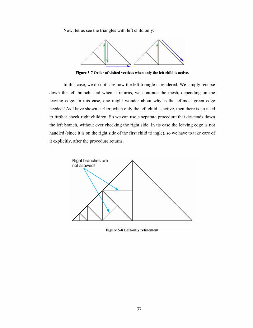
Now, let us see the triangles with left child only:
Figure 5-7 Order of visited vertices when only the left child is active.
In this case, we do not care how the left triangle is rendered. We simply recurse
down the left branch, and when it returns, we continue the mesh, depending on the
leaving edge. In this case, one might wonder about why is the leftmost green edge
needed? As I have shown earlier, when only the left child is active, then there is no need
to further check right children. So we can use a separate procedure that descends down
the left branch, without ever checking the right side. In tis case the leaving edge is not
handled (since it is on the right side of the first child triangle), so we have to take care of
it explicitly, after the procedure returns.
Figure 5-8 Left-only refinement

38
Processing triangles with right child only is quite similar:
Figure 5-9 Refinement when only the right child is active
First we render the left side as shown in Figure 5-9, and then we recurse down
the right branch. This recursion will also be a restricted one, going right only. However,
since this is a tail recursion, it can be rewritten into a simple loop, and then inlined,
totally eliminating the function call overhead (together with stack maintenance), making
the implementation even more efficient.
Now, the only case left out is when both children are active:
Figure 5-10 The simplest case is when both children are active.
In this case, all we have to do is recurse down the left side, insert the vertex at
the apex and the continue down the right side. We do not have to care about which
edges are incoming or outgoing, everything will be handled autmatically by the
recursion calls.
Now that we have covered all of the possible cases, implementing the set of
refine functions (a general, a left only and a right only) should not be hard. Note that in
all of the cases above, we now exactly what vertices need to be checked and in what
order they have to be appended to the triangle strip. So, although the code is longer,
since we have prepared to deal with every possible cases, we do not have to explicitly
check against degenerate vertices any more. This makes this algorithm more effective
than the original.
Empirical results show that while the original algorithm generates strips that
require 1.56 vertices per triangle, my enhanced method generates the same mesh with
only about 1.32 vertices required per triangle. In reality the speed improvements are
rarely noticeable when using indexed primitives, since these extra vertices are all
39
degenerates, and thus can be specified with a single index value. An index does not take
up considerable space, and it also utilizes the GPU’s vertex cache (i.e. no transformation
is required). Even if we do not use indexed primitives, the GPU’s T&L stage is rarely
the bottleneck. The real strength of the algorithm lies in the fact that it checks less
inactive vertices during refinement. Since in my work I require some more excessive
calculations per vertex (see later in Chapter 6), it is very important that no vertices are
processed unnecessarily.
5.2 Lazy view-frustum culling
The hierarchical culling of the bounding spheres against the view-frustum is a
very efficient method for rejecting large chunks of vertices, early in the refinement.
Spheres outside a plane are rejected, spheres inside all planes are accepted without
further testing. This method works very nicely, but there are some subtle problems.
First, it is possible to cull away a vertex in the lowest level, that was part of a triangle,
thus rendering a coarser triangle. This results in popping (most noticeable at the near
clip plane of the view-frustum). Since this popping is the result of vertex culling, using
geomorphing does not help. Although this popping is usually not disturbing, there are
cases when it results in a serious error (see color plates at page 66). This is not
acceptable and should be eliminated. The original paper suggests inflating the bounding
spheres until they enclose their parents. However, there is another problem with
efficiency. While culling away thousands of vertices with one sphere is very efficient,
culling small numbers (or even individual!) vertices at the lower levels is rather
inefficient. I propose that at the lower levels, culling should be stopped, and all vertices
accepted automatically (as if they were inside the frustum). This eliminates the popping
artifacts, and also results in a relative speedup, since the GPU does a far better job of
culling individual vertices than the CPU. Note that this does not affect gross culling,
since the majority of vertices are culled away high up in the hierarchy. Only vertices on
the lower levels and near the clipping planes are affected. This method has its own
problems, however, as it does not guarantee mesh continuity outside the viewing
frustum (Figure 5-11). This should not be a problem for most applications, since mesh
continuity is only required when building the mesh asynchronously in a separate thread.
In such cases frustum culling is likely to be skipped alltogether, allowing the camera to
turn around freely and still see a detailed mesh, while the other thread is busy building
the new mesh.

40
Figure 5-11 Culling the bounding spheres against the view frustum.
The shaded area indicates the inner side of the frustum.
We should investigate the figures above to have a better understanding of what
happens when culling the spheres against the viewing volume, and why the new method
causes cracks outside the frustum. For the sake of simplicity let us assume that the
projected error is bigger than the threshold for every vertex (i.e. all vertices are active,
unless culled). Using the original algorithm, only the spheres not intersecting with the
viewing volume are culled. This means that the vertex with the smallest bounding
sphere on the lower left figure will be culled, coarsening the triangle compared to the
lower right figure. This coarsening does not happen on higher levels because the sphere
hierarchy is loose enough to enclose the whole triangle. Lazy culling eliminates this
popping, since the vertex will be active, even if its sphere is outside the viewing volume
(because its parent intersects the volume). However, this will result in a T-vertex on the
upper right figure, where the lowest level is activated, but only one of its parents are
really active. In the next chapter we will see how the idea of lazy culling fits very nicely
with the method for adding detail geometry.

41
6 Extending SOAR with detail geometry
6.1 Overview
Although SOAR is a very powerful terrain rendering framework, it has some
severe limitations. It can only handle a fixed resolution, static terrain. The main reason
for these limitations is that the algorithm is heavily dependent on precomputed data (the
per vertex bounding sphere radius and the object space error), that can not be computed
in real-time.
Fixed resolution means that the amount of detail is limited. Even though the
algorithm itself could deal with huge, detailed terrains, storage and preprocessing
requirements quickly grow beyond a limit that makes it impractical for most
applications. Obviously, if we were about to display only geometry that is based on true
measured terrain data, then there is nothing we could do. But in most cases, the extra
detail’s sole purpose is just adding another level to the illusion of reality. Usually, these
tiny details cannot even be measured by conventional methods. So some form of
parametric description would be best for such details. The parameters should describe
soil properties, like roughness, and such. This would make it possible to define different
details for different kinds of terrains.
Static terrain means that it is not possible to change surface geometry on-the-fly,
without recalculating a lot of data. For every changed vertex, its radius and error must
be recomputed and propagated upwards, through its ancestors, until the nesting
requirement is met. Note that this simple propagation only works for incremental object
space errors measured between consecutive levels of refinement. With other error
metrics, the position change of one vertex could affect the errors of many other vertices
(usually the whole terrain), making it impossible to recalculate every frame. If we stick
to incremental errors, then this propagation might be acceptable for animating a couple
of vertices every frame. However, animation of larger areas are not possible.
In this section I am going to introduce a simple method that enables us to add
more detail to the surface and to even have dynamic detail (as it will soon turn out, the
requirements for the two are quite similar).

42
6.2 Basic concepts
There are countless methods to generate procedural detail. Perlin noise is one of
the most popular techniques, because it is easy to compute and can give continuous,
non-repeating, infinite detail. However, calculating the error term and bounding spheres
for such procedural detail is very hard, if at all possible. In a sense, such procedural
detail can be thought of as dynamic geometry (they both lack the required information).
For the sake of simplicity, I will use a precomputed tileable detail map instead, and
apply that onto the base geometry. From now on, I will call the original terrain
heightfield the base map and the one containing the detail the detail map.
In order to increase detail, we have to increase the virtual grid resolution of the
terrain. This means that we have to add extra
levels to the refinement. Figure 6-1 illustrates how
this happens: blue vertices represent the base map
and orange vertices represent the detail map. Next
we have to find a way to embed the actual
geometry into these extra levels, so that the new
vertices on the grid are assigned proper position
information. Besides the position, object space
error and bounding sphere radius are also
required. Since we are using a precomputed detail
map, we have all these information at hand. This
may all sound easy, but there are a cuple of caveats. Great care must be taken to insure
that these properties will remain valid and nested after the extra detail is mapped onto
the original map.
6.3 Detailed explanation
There are several different ways to combine surfaces together. We could use
displacement mapping, or just simply add the two maps (their height values) together.
There is a problem, though. Namely that these maps are not continuous (the points are
defined at discrete intervals) and they are defined at different resoultions. So, first we
would have to interpolate the lower resolution base map, then apply the detail with
whaterver method we have choosen. There are many kinds of interpolation methods,
each having its own strengths and drawbacks. The cheapest and easiest one is linear
Figure 6-1 Embedding detail map

43
interpolation. In our case, since we are dealing with a surface, we would have to use
bilinear interpolation. Using the notations on Figure 6-1, the interpolated value could be
calculated like this: ( ) ( )( ) ( ) ( ) xyHyxHyxHyxHyxH 3210 1111, +−+−+−−=
If we introduce the two vectors:
[ ]( )( ) ( ) ( )[ ]xyyxyxyxc
HHHHh−−−−=
=1111
3210
then the result can be written as a simple
dot product: ( ) hcyxH =, . This is good,
since usually we will have to interpolate
many values at a time (position, normal,
gradient, color and possibly some other
miscellaneous attributes) and can reuse the
c vector. Also, these kinds of vector
operations can be done quickly using
SIMD (Single Instruction Multiple Data)
instructions.
Now that we know how to interpolate our surface, we should decide about
which combining method to use. Note that a surface usually cannot be mapped onto
another surface without distortions. The simplest example is when we try to map an
image (defined on a plane) onto an arbitrary
surface. Or, thinking the other way around,
when we try to map a surface (e.g. a sphere)
to a plane. Looking at Figure 6-2 we can
compare displacement mapping (on the
middle) with simple addition (on the right).
Since our detail geometry usually have little
or no real physical meaning, distortion is not
a problem. In fact, distortion is good, since it
makes tiling of the detail map less noticable. Simple addition is also much simpler to
compute, which is essential for a real-time algorithm. Combining the height values is
the easiest part. Much more problematic is the computing of normal vectors for the
resulting surface. It is easy to see that normals cannot be simply added together. Since
normal vectors are most important for lighting the terrain, I leave its discussion to the
Figure 6-2 Bilinear interpolation
Figure 6-3 Comparing surface combining
techniques.
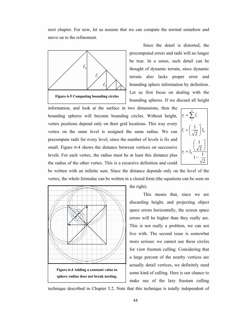
44
next chapter. For now, let us assume that we can compute the normal somehow and
move on to the refinement.
Since the detail is distorted, the
precomputed errors and radii will no longer
be true. In a sense, such detail can be
thought of dynamic terrain, since dynamic
terrain also lacks proper error and
bounding sphere information by definition.
Let us first focus on dealing with the
bounding spheres. If we discard all height
information, and look at the surface in two dimensions, then the
bounding spheres will become bounding circles. Without height,
vertex positions depend only on their grid locations. This way every
vertex on the same level is assigned the same radius. We can
precompute radii for every level, since the number of levels is fix and
small. Figure 6-4 shows the distance between vertices on successive
levels. For each vertex, the radius must be at least this distance plus
the radius of the other vertex. This is a recursive definition and could
be written with an infinite sum. Since the distance depends only on the level of the
vertex, the whole formulae can be written in a closed form (the equations can be seen on
the right).
This means that, since we are
discarding height, and projecting object
space errors horizontally, the screen space
errors will be higher than they really are.
This is not really a problem, we can not
live with. The second issue is somewhat
more serious: we cannot use these circles
for view frustum culling. Considering that
a large percent of the nearby vertices are
actually detail vertices, we definitely need
some kind of culling. Here is our chance to
make use of the lazy frustum culling
technique described in Chapter 5.2. Note that this technique is totally independent of
Figure 6-4 Adding a constant value to
sphere radius does not break nesting.
Figure 6-5 Computing bounding circles
211
21
21
0
0
−
=
=
= ∑∞
i
i
i
i
iii
lr
ll
lr

45
vertex positions, making it useful for even culling dynamic geometry. If we do not want
to waste many vertices, we could inflate the real bounding spheres (Figure 6-5), so that
the lowest level spheres contain all of their vertices’ detail descendants.
The next question is how we can assure the nesting of the projected errors. We
have two choices. For static detail, we could simply use the precalculated nested object
space errors and accept the fact that they will be somewhat inaccurate because of the
distorted geometry. Or we could just use a constant error for every detail vertex (this
works for both static and dynamic detail), effectively making LOD selection distance
based only. This is usually not a serious disadvantage, since detail geometry tends to be
featureless, noise like, so the error is likely to be nearly the same for most vertices. Still,
we have to make sure that the projected error will be nested with regards to the vertices
in the original base mesh. This could be solved by projecting the error from both the
real bounding sphere and the bounding circle assigned to the vertex’s level, and take the
maximum of the two errors and compare that against the threshold. This might seem to
be very inefficient, because of the double work, but if the first calculated error is bigger
than the threshold, then we do not have to check the other projection. Clearly, for detail
level vertices we only have to make the horizontal projection only.
Since we are dealing with multiple separate maps, special care must be taken to
insure error nesting between maps (only if the detail geometry has error information of
course).

46
7 Terrain lighting
7.1 Overview
Up until this very moment, we have been dealing exclusively with the
geometrical description of the terrain surface. We have shown how to build a near
optimal triangle mesh that approximates the surface geometry as seen from a given
view. Now it is time to investigate how these triangles actually get turned into colorful
pixels on the screen. What follows is a brief description of the OpenGL1 rendering
pipeline, but this basically applies to every other method based on incremental image
synthesis. Each of the primitives (in our case triangles) are defined by their vertices in
object space. Each vertex can be assigned a number of attributes like position, surface
normal, texture coordinates, material properties (like primary and secondary colors) and
so on. These vertex attributes are first transformed by the T&L (transform and lighting)
stage. This usually includes transforming position and normal vectors to eye space, and
calcuating various light contributions that change the vertex’s colors. Then the position
vector is projected to clip space, and the primitive is clipped in homogeneous
coordinates. After clipping, perspective division is applied, resulting in normalized
device coordinates, which is further scaled and biased by a viewport transformation to
obtain window coordinates (including depth). Using these window coordinates, the
primitives are then rasterized. During rasterizing, each pixel inside the primitive is
visited, and assigned a fragment. Fragments contain a lot of important information like
color, depth, stencil values, texture coordinates and so on. Most of these properties are
computed using perspective correct interpolation along the primitive. If all of the per
fragment visibility tests (like the ownership, scissor, stencil, depth and alpha tests) are
passed, then the pixel is finally assigned a color value that can be stored in the color
buffers and displayed on the screen. Which part of the rendering pipeline should be
called lighting is not obvious. Formerly all calculations regarding light contributions
had been computed per vertex in the (as its name suggests) T&L stage, but today the
rendering pipeline is much more flexible. It is possible to define complex per fragment
operations to compute each pixel’s color individually. I try to be as generic in my
1 The cross-platform industry standard graphics API, see [14].

47
definition as possible, so when I say lighting, I am talking about the whole setup of the
rendering pipeline.
Lighting can have a great influence on how the final image will look like. For
example setting every pixel of the surface to the same color can still be thought of as
some kind of (admittedly very trivial) lighting. However, such lighting will not help us
(as a viewer) much. We would see a solid color covering most of the screen, no matter
how detailed the geometry is. On the other hand, if we could calculate the reflected light
based on some physical model, for each pixel, the result could be a much more
believable, almost photorealistic image. So our goal is to find an efficient method to
perform quality lighting real-time.
Most presented terrain rendering algorithms deal only with the surface’s
geometric description, they usually do not care much about lighting1. The reason for this
is that lighting should be independent of how the geometry is built up. While this is
true, most lighting computations require a substantial amount of geometrical
information. Since we are dealing with CLOD algorithms, we throw away a lot of
supposedly unnecessary detail. The truth is that we do throw away important details. In
the error metrics, we use vertex positions exclusively, completely ignoring materials
and other surface properties. This results in poor approximation of visual appearance. If
we did take them into account, however, we would possibly have to tesselate down to
pixel sized triangles, to achieve sub-pixel accuracy, which is clearly not possible in real-
time. Still, our ultimate goal is precise per pixel shading of the terrain. To achieve this
we would need a normal vector for every fragment. Now it can be seen that we have to
find a way that is efficient and works with LOD meshes. Using detail geometry makes
things even more difficult. Extracting normal vectors from a complex surface, that was
combined from several heightmaps is not trivial.
In the following section, I am going to introduce basic and advanced lighting
methods. After that I will introduce some techniques that make it possible to light such
a detailed terrain.
1 There are several separate works though, that investigate terrain shadowing and the effect of
light scattering in the air.

48
7.2 Lighting basics
The physics of real-world lighting is quite complex. Radiometry, photometry
and colorimetry are not discussed here (refer to [11], [12] for details on these subjects).
We use a simplified model instead, to simulate lighting. In this model we can think of
lighting as photon particles emitted from lightsources. These particles bounce between
objects in the scene, until some of them arrive in the eye. Only those particles that are
absorbed by the eye contribute to the final color of a pixel. It is easy to see that the color
of one pixel is usually affected by the whole scene. So computing the color of a pixel
would require thorough traversing of the full scene (for this reason this is called a global
lighting solution), which is usually prohibitively expensive for real-time rendering. For
this reason, we have to further simplify our model, by using a local lighting solution
instead. This means that each primitive is shaded independently, as if it was alone in the
scene. This way, light is coming directly from the lightsources. Indirect lighting
reflected off from other surfaces and shadows cast by other objects are ignored in this
model. However, it is still possible to approximate environmental reflections and
shadows by using some clever techniques.
How a particle bounces off a surface depends on the surface’s material. Material
can be thought of as a function that gives the spectrum of light that is reflected in a
given direction, depending on the incoming light. Finding a compact and accurate
representation that describes a surface’s material properties at each point is not an easy
task. Evaluating such a complex function can also be very expensive. This is the reason
why phosphorescence, fluorescence, and light scattering inside an object are discarded
even by high quality off-line renderes. A very good material description is offered by
BRDFs (Bidrectional Reflectance Distribution Function). However, BRDF is still not a
widely used technique. The most common way to describe a material is to give its
ambient, diffuse and specular reflection terms. These terms determine how much of a
particular type of light is reflected by the surface. Ambient illumination simulates
scattered omnidirectional light. It has no source, comes from every direction, and is
reflected evenly in all directions. Diffuse light is also reflected equally in every
directions, but its intensity depends on the incoming angle. Using the notation on Figure
7-1, it can be calculated by computing a dot product between the normal and light
vectors. Specular light simulates highlights on shiny objects. Its intensity also depends
on the incoming light angle, just as it is with difffuse lights, but it is reflected back only

49
in a particular direction. So, how much of it reaches the eye depends also on the
viewer’s direction. A shininess factor is used to determine how focused the reflection is.
There are a couple of ways to
calculate a light’s specular
contribution, a popular one is
Blinn-Phong model, which
calculates the dot product
between the light direction and
the halfway vector (see Figure
7-1), and raises it to a power of
shininess to make distribution
more or less focused. To obtain
the final reflected colors, the
ambient, diffuse and specular
factors must be modulated by the corresponding material and lightsource intensities,
and then added together. Sometimes an emissive term is also added to simulate surfaces
that emit light themselves. The result is clamped to a dynamic range (usually 0..1). This
means that high intensity lights may saturate into white.
These material properties could be defined as simple color values per object or
per vertex, or could be stored in a texture map and stretched over an object, effectively
resulting in per pixel material resolution. Obviously, the complexity of the per fragment
operations that can be effectively calculated depends on the capabilities of the graphics
hardware.
Now we have to describe the lightsources. In our simplified model, there are two
main types of lights: positional lights and directional lights. The basic positional light
(also called a point light) emits light in every direction, its intensity is usually attenuated
over distance. There is also a special positional light, the spotlight, which has some
additional constraints like a direction vector, cutoff angle and falloff factor that modifies
the emitting direction. Directional light, on the other hand is assumed to be infinitely far
away (and thus also called infinite light), and for this reason the incoming light can be
considered parallel. Since the light direction is constant for the whole screen, direction
lights are much cheaper than point lights (for which the direction vector always have to
be recalculated). Obviously, attenuation have no meaning for lights that are infinitely far
away. A good example of a directional light is the Sun.
Figure 7-1 Most lighting calculations require these unit
length vectors. n: surface normal l: light direction
e: eye direction, h: halfway vector (l+e)

50
There are also some very nice tricks that can simulate much more complex
lightsources. The main idea is to use a texture to capture lighting effects (as we have
done it with materials). The simplest example is capturing diffuse lighting in lightmaps.
These intensity textures hold the amount of light that strikes the surface. Such a map
can then be stretched over a surface and modulated with its diffuse color. The lightmap
does not have to be statically linked to a surface. Using projective texturing, a lightmap
could be projected over any surface to simulate a spotlight for example. Going further,
we could render colorful lights into a cube texture map to simulate just about every kind
of point lights. Also, we could use the cube map to capture the environment as it is seen
from a point (this is called an environment map). This enables rendering of surfaces that
reflect their environment. It is also possible to capture the overall ambient and diffuse
light contributions for every direction in an irradiance map. The difference between an
environment map and an irradiance map is that while the first gives the incoming light
intensity from a single direction, the second integrates light contributions coming from
every direction. Using these powerful techniques, it is possible to render radiosity
quality images. Obviously, there is some cheating in using cube maps for such effects.
They contain a snapshot of the surrounding environment as seen from one point in
space. Ideally, we would need a different cube map for every point in space. In practice,
one cube map is enough, however, if the environment is relatively far. Obviously, for
dynamic scenes, we would have to recompute these cube maps.
The possibilities of using texture mapping are endless. For example calculating
an attenuation factor for every pixel is very expensive, instead we could use a projected
3D intensity texture as a look-up table for distance based attenuation. Such a texture
could also be used the same way to achieve stunning volumetric lighting effects.
As I have stated earlier, shadows are not handled by local lighting models
automatically. There are many popular methods that can be used, though, including
stenciled shadow volumes and shadow mapping (also called shadow buffers). However,
I am not going to describe them in more detail here. Refer to [11][13] for more
information on the topic.

51
7.3 Per pixel dynamic lighting of detailed surfaces
For now, we do not have to care about materials, nor light properties (these are
the parts that are independent of the geometry). First, we should only be concerned
about having correct surface normals for the detailed terrain at every pixel, even where
geometry is not tesselated enough. The trivial solution would be to precompute a texture
map that holds normal vectors for the detailed terrain, and stretch this map over the
surface. Obviously, this is impractical, considering the resolution of the combined
terrain1. The other solution would be to combine the base and detail maps at run-time to
compute the normal vector at a given fragment. These calculations should be done in a
vertex independent manner, to avoid dependency on geometry LOD level.
The original concept of bump mapping is supposed to solve exactly these kinds
of problems [15]. A bump map (what is actually a heightmap) is defined to displace the
underlying surface, but instead of actually tesselating and displacing the geometry, only
the surface normals are perturbed by the bump map in a way, that the resulting vector is
the normal for the corresponding displaced surface. So it seems like, as if the surface
geometry has been displaced, when in fact it is not. Obviously, this lighting trick does
not work for silhouette edges, so it cannot replace geometry totally. Still, it is good
enough for simulating relatively small bumps on the surface. Our case is somewhat
different, since we do not want to replace all the detail geometry with bump maps. We
just want to use the concept to generate normals for per pixel lighting of the surface.
Nearby regions will have real geometry, but for far away parts of the terrain, the extra
lighting will make up for the lack of detail.
Although the original idea is quite old (it has been invented in 1978 by James
Blinn), it is still too expensive to compute the normals for displaced surfaces real-time.
Simplified versions of the original approach are widely used, though. By assuming that
the bump map is defined in tangent space, the required computations become much
more manageable. This assumption means that no combining is required, since the
bump map is independent of the base surface. Of course this also means that the lighting
calculations must be taken place in tangent space. So, for each triangle in the mesh, we
have to calculate its tangent space basis vectors, and transform the lightsources to
tangent space. However, that triangle is usually just an approximation of the real
1 Paging in the huge texture from mass storage devices, using clipmapping might work, but it is
not practical in any way.
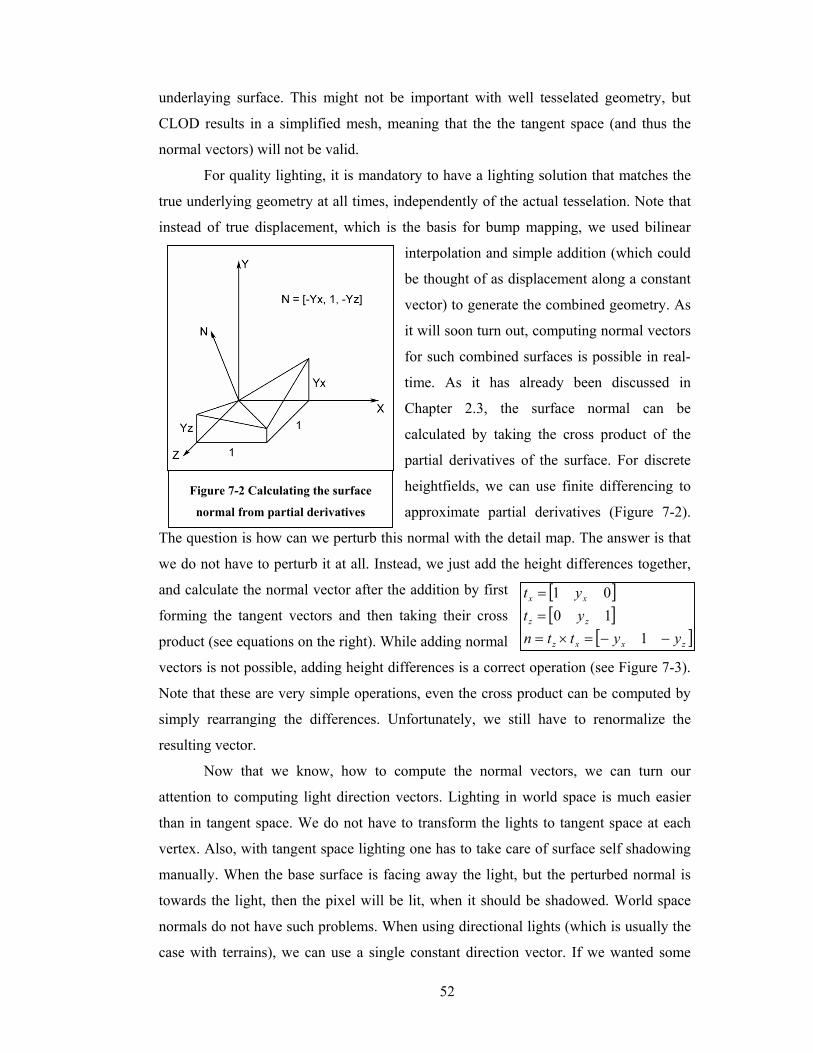
52
underlaying surface. This might not be important with well tesselated geometry, but
CLOD results in a simplified mesh, meaning that the the tangent space (and thus the
normal vectors) will not be valid.
For quality lighting, it is mandatory to have a lighting solution that matches the
true underlying geometry at all times, independently of the actual tesselation. Note that
instead of true displacement, which is the basis for bump mapping, we used bilinear
interpolation and simple addition (which could
be thought of as displacement along a constant
vector) to generate the combined geometry. As
it will soon turn out, computing normal vectors
for such combined surfaces is possible in real-
time. As it has already been discussed in
Chapter 2.3, the surface normal can be
calculated by taking the cross product of the
partial derivatives of the surface. For discrete
heightfields, we can use finite differencing to
approximate partial derivatives (Figure 7-2).
The question is how can we perturb this normal with the detail map. The answer is that
we do not have to perturb it at all. Instead, we just add the height differences together,
and calculate the normal vector after the addition by first
forming the tangent vectors and then taking their cross
product (see equations on the right). While adding normal
vectors is not possible, adding height differences is a correct operation (see Figure 7-3).
Note that these are very simple operations, even the cross product can be computed by
simply rearranging the differences. Unfortunately, we still have to renormalize the
resulting vector.
Now that we know, how to compute the normal vectors, we can turn our
attention to computing light direction vectors. Lighting in world space is much easier
than in tangent space. We do not have to transform the lights to tangent space at each
vertex. Also, with tangent space lighting one has to take care of surface self shadowing
manually. When the base surface is facing away the light, but the perturbed normal is
towards the light, then the pixel will be lit, when it should be shadowed. World space
normals do not have such problems. When using directional lights (which is usually the
case with terrains), we can use a single constant direction vector. If we wanted some
Figure 7-2 Calculating the surface
normal from partial derivatives
[ ][ ]
[ ]zxxz
zz
xx
yyttnytyt
−−=×===
11001

53
positional lights, then we had to calculate the direction vector per vertex, but it is a
cheap operation compared to
transforming to tangent space.
The light vector is interpolated
along the triangle, just like other
per vertex attributes. This
interpolation results in non unit
length vectors that would make
the shading darker in the center
of the triangle. We can normalize
the vector by feeding it as texture
coordinates for a normalization
cube map. The same technique
works for other direction vectors, like the local viewer (or halfway vector, depending on
the model used for calculating the specular term)
Now we have to find a way to do the actual combining with available hardware.
We precompute the height differences and store them in separate base and detail texture
maps. Using multitexturing, we can stretch these textures over the surface. Note that
this mapping requires filtering of the texture map. The simple bilinear interpolation for
magnification, and box filtering for mipmapping produces correct difference values,
since we used the same method for interpolating the geometry.
If we have a graphics hardware that supports fragment programs (Radeon 9700
or GeForceFX class GPUs), then we can write a simple fragment program that adds the
texels, forms the normal vector, and normalizes it using pure arithmetic operations.
Since all operations are done using floating point arithmetics, the result is accurate
surface normal. Alternatively, normalization could be done using a dependent texture
lookup into a normalization cube map, which might be a bit faster in some cases.
Computing the dot product between the normal and the light direction vector results in
the diffuse term. Modulating it with the diffuse color gains the final color.
Unfortunately GeForce3 class hardware do not support fragment programs, nor
dependent texture fetches in the combiner stage. This means that it is not possible to add
two textures and do a dependent texture read after that, in the same pass. Still, it is
possible to make the necessary computations using a multi-pass technique and a special
lookup texture. In the first pass we render the terrain to an off-screen pixel buffer using
Figure 7-3 Adding differences. Note that these are
signed values (ie. df is negative in this case).

54
additive texture environment mode1 to add the texels that represent the height
differences. In the second pass, we render the terrain again, but this time to the on-
screen window. We use the pixel buffer that was created in the previous pass as a
texture projected onto the screen to perform dependent texture read using the texture
shaders. The two difference values index into a precomputed texture map that contains
the unit length normal vectors (encoded as RGB values) for the corresponding
differences. We then compute the dot product between the normal vector with the unit
length light direction vector (that is provided by a cube map as described earlier), using
dot3 texture environment, to get the diffuse contribution for the fragment. Modulating
this value with the diffuse color specified by a texture bound to the fourth texturing unit
could be used to specify the final color of the fragment.
If the scene contains only static directional lights, than the diffuse contribution
could be baked in the lookup texture instead of normal vectors, saving a dot product
operation (and also requires less texture space, since it is an internsity value instead of a
three component vector).
If the per fragment operations are too expensive then there is an optimization
technique that works for both of the methods above. First we render the scene with
depth writing and testing enabled to lay out the depth buffer (and, optionally render the
diffuse color at the same pass). Then we turn off depth writing and use depth testing
only (which is a very cheap operation on decent hardware) to skip invisible fragments in
the following passes. This saves a lot of unnecessary per fragment calculations.
The method introduced here is efficient, easy to implement, and results in
correct normal vectors at each fragment, representing the true geometry, independently
of the actual tesselation.
1 Every time I write texture environment, it can be done with register combiners instead. I stick
to using environment modes when possible, because it is more standard.
55
8 Implementation
8.1 Overview
Personal computers are so complex and diverse, that it would be impossible to
develop software without some powerful tools. Today, there are mature compilers that
produce very good, optimized machine code for many different processor architectures.
Also, the operating system supports industry standard APIs (Application Programming
Interface) that enable easy access to special hardware capabilities from high level
languages. It seems that everything is given to produce high performance applications
that work on a range of different personal computers.
However, the computing performance of personal computers grow at an
astonishing rate. Graphics accelerators are evolving even faster than other components
of the PC. The market can hardly keep up with the pace of advancement in technology.
We can see graphics cards on the shelves that are three generations away from each
other. Even the graphics APIs can barely keep up with the changes. Fortunately, the
OpenGL API has an extension mechanism that allows new features to be published
quickly by hardware manufacturers, not having to wait for a new version of the API. Of
course, this means that to utilize the latest features, sometimes vendor specific
extensions have to be used, which makes the software not portable. This is not a serious
problem, though, since in the long run, these extensions will likely to be merged into the
core API, ensuring that the method is portable across various hardware accelerators.
Today, personal computers are based on the IA-32 family of processors.
Although these family of processors have a standard instruction set, we can see similar
extensions as with graphics cards. Recent CPUs have special SIMD (Single Instruction
Multiple Data) instruction sets that can speed up many computationally intensive
applications. Unforunately, since these instructions are not in the core instruction set,
not all processors supports them. Different processors have different instruction sets for
the same task! Intel has SSE (Streaming SIMD Extensions), while AMD has 3DNOW!
giving roughly the same functionality. Fortunately, newer AMD processors (starting
from the AthlonXP) support the 3DNOW! Professional extension, which is in fact the
original 3DNow! extended with Intel’s SSE instruction set. These extensions are not

56
supported directly by compilers, but they offer so much additional performance, that it
would not be wise to discard them.
When researching new, cutting edge technologies, one should not target legacy
hardware and legacy functionality. It does not make sense to support them, because
most of the time they require a totally different approach to the same problem. So I
decided to define a strict minimum hardware requirement for the sample software, and
tried to make sure, that this hardware is utilized to its maximum.
8.2 The framework
Although the goal of this work is to develop a high performance terrain
rendering application, such software requires a lot of supporting code for window and
input management, journaling, scripting, timing, camera handling and so on. These
features are required by most similar applications and are thus independent of the actual
terrain rendering algorithm. Such features are best implemented in a separate, portable
framework.
The framework has a well defined interface, that allows different components to
use the services offered by it. A component can even register itself as an additional
service, making it easy to further extend the framework. Such component based systems
have a lot of advantages. Given a well defined interface, it is possible to develop
different parts of the system independently. This makes developing huge, complex
software manageable. Components can also be swapped in and out of the framework, or
replaced (even runtime) without any modification required to the other components.
This independency also helps keeping down build times, which is very important for
large projects.
8.3 The preprocessing module
The terrain preprocessing module reads any non-interlaced 16bit per channel
grayscale PNG (Portable Network Graphics) file and converts it to a preprocessed
terrain data file. Preprocessing is a lengthy operation, it calculates relative object space
errors, nested bounding spheres, and gradients for every vertex.
The demonstration program uses the Puget Sound dataset (Washington state,
USA) with 160m horizontal and 0.1m vertical resolution. The base grid is made up from
1024x1024 points, meaning that the map size is roughly 160km x 160km. This base
map is enhanced with another 1024x1024 detail map (a simple tileable pattern), that is

57
embedded into 16x16 sized partitions in the base map. This means, that each 1x1 quad
in the base map is subdivided to 64x64 vertices. This results in an effective resolution of
65536x65536 height samples, meaning that the horizontal resolution is 2.5m! Note that
these numbers are for the actual sample dataset, and that the program itself could handle
maps with any other size. Since the rendering algorithm is output sensitive, it scales
easily for even more detailed terrains.
I used the built in embedded script language (Lua) of the framework to enable
easy configuration of terrain parameters.
8.4 The rendering module
The terrain data is paged in from disk using the file mapping services offered by
the operating system (MapViewOfFile in the Windows API). This service maps a file
into linear address space. Although this would make it possible, to work with huge
maps that do not even fit into the physical memory, the simple linear scheme I used for
data access makes it impractical to use very large maps. The reason for this is that such
linear data access has very poor spatial locality, and introduces a lot of page faults,
making it only useful for in-core rendering. By using the somewhat more complicated
hierarchical quadtree method described in [1], it would be possible to use out-of-core
rendering for such large maps. Also, it is worth noting that today’s computers are
usually limited by memory throughput, so this cache friendly memory access pattern
should speed up even in-core rendering considerably. There is still a lot of research
going on to find even more efficient data layout schemes.
Due to lack of time, I have not implemented per pixel lighting of the detailed
surface. The demonstration engine only uses per vertex lighting. However, it uses the
same mathematics to compute the normals, what means that I had to interpolate
difference values and compute normals using the CPU. The result is that the rendering
performance is very much CPU limited. Also, lighting is not nearly as detailed as it
should be, because of the CLOD geometry. By implementing per pixel lighting, the
performance will likely to go up, besides the increase in image quality.
To perform view-frustum culling during refinement, it is necessary to extract the
six clipping planes from the combined model-view-projection matrix. I have used the
very elegant method described in [16] to do this.
I used depth clamping (as described in section 4.6.3) to achieve better depth
resolution.

58
In order to minimize memory bus usage, I have used the vertex array range
extension that supports writing directly into AGP or local video memory, avoiding
unnecessary copying to and from generic system memory. This is most efficient for
multipass rendering, since we do not have to resend the vertex arrays every time. I used
this technique together with the fence extension that enables asynchronous processing
of the vertex arrays.
The sample implementation modulates the vertex lit triangles by a simple 3D
noise texture to help perceiving of perspective. I used hardware texture coordinate
generation to avoid sending texture coordinates. Normalizing is also done in the
hardware T&L stage, to further save CPU cycles.
8.5 Testing environment and performance
The sample implementation have been tested on an average desktop PC. Details:
• Processor: AMD AthlonXP 1800+ (1533Mhz)
• Memory: 512MB PC2700 (333MHz DDR)
• GPU: nVidia GeForce4 Ti4200 128MB
• OS: Microsoft Windows XP Professional
Measuring and comparing the performace of different terrain rendering methods
is difficult. It is not possible to give precise and comparable numbers, because of the
wealth of parameters that affect visual appearence and thus performance. Since visual
quality is subjective, it is not fair to compare the results of different methods. For
example pure distance based detail geometry is faster and works well for detail
geometry with noise like distribution. On the other hand, error based detail geometry
might require less triangles to achieve the same visual quality at the expense of
additional computing overhead.
The algorithm is clearly CPU limited, since increasing the window size and
doing multiple passes does not affect performance at all1. Performance varies heavily
depending on the geometry level of detail settings. Also, measuring frames per second
is not a good performance indicator, because this number varies based on the viewpoint.
1 Note that increasing window size should mean that more vertices are required to result in the
same screen space error, but I used a projected metric for a fixed resolution window to avoid these
differences during testing.

59
Instead, I measured triangle throughput for the best and worst cases. In the best case I
measured pure refinement speed with simple distance based error, without culling. The
result is roughly 9 million triangles per second. This is quite good for dynamic mesh
generation. However, when doing proper error metrics calculation, together with view
frustum culling and detail geometry calculations (terrain interpolation, and normal
generation), performance drops to about 2.3 million triangles per second. As stated
earlier, using per pixel lighting stresses only fillrate, and would save a lot of
calculations that are done by the CPU on this implementation. Also, implementing a
datastructure with better cache locality would likely to increase performance even more.

60
9 Summary
I have successfully developed and implemented an algorithm that supersedes the
refinement and frustum culling methods introduced by the original SOAR algorithm. I
also showed how this new frustum culling technique, together with static bounding
circles, enables adding detail to the original geometry. As a complement for geometry, I
also developed an efficient method to perform accurate per pixel lighting of this large
and detailed terrain, independently of the geometrical resolution of the output mesh. The
result is a robust method that enables rendering and shading of vast surfaces in real
time.
However, this is just the first step in creating truly realistic visualization of a
detail rich terrain. There is still a lot of challenge ahead. Ultimately, what we would like
to see, is not just a bare surface, but a scenery full of nature’s wonders. There are a lot
of other aspects of realistic terrain visualization that we have not talked about in this
paper. Terrain self shadowing makes the scene much more convincing, and can be
accomplished by horizon mapping [8]. More realistic lighting (that depends on the time
of day and the weather) could be achieved by taking into account the light scattering in
the air [9]. Volumetric fogging, clouds and other environmental and weather effects
would increase reality even further. Particle systems could be used to simulate fire, dust,
wind, snow and rain. Modelling of ecosystems is also very important for a natural
appearance [10]. Flora (trees, bushes, grass) could be selected based on some kind of
quadtree structure and rendered using impostors. Integrating portal based visibility
culling into the terrain rendering algorithm would enable combining of large outdoor
areas with indoor areas (like a house). Hardware displacement mapping coul be used to
add even more dynamic detail, like sand, or snow.
The list of possible enhancements is practically endless. Now we can see that
there is a long way ahead for someone aiming at real-time visualization of natural
looking terrains. I can only hope that the methods and ideas introduced in this paper will
serve as a basis to some techniques that will present an even richer visual experience.

61
10 References
[1] P. Lindstrom, V. Pascucci: Visualization of Large Terrains Made Easy [2001]
[2] P. Lindstrom, V. Pascucci: A General Framework for View-Dependent Out-of-
Core Visualization [2002]
[3] P. Lindstrom et al.: Real-Time, Continuous Level of Detail Rendering of Height
Fields [1996]
[4] M. Duchaineau et al.: Real-Time Optimally Adapting Meshes [1997]
[5] H. Hoppe: Smooth View-Dependent Level-of-Detail Control and its Application
to Terrain Rendering [1998]
[6] R. Pajarola: Large Scale Terrain Visualization Using The Restricted Quadtree
Triangulation [1998]
[7] T. Ulrich: Rendering Massive Terrains Using Chunked Level of Detail Control
[2002]
[8] P.P.J. Sloan, M.F. Cohen: Interactive Horizon Mapping
[9] N. Hoffman, A. J. Preetham: Rendering Outdoor Light Scattering in Real Time
[10] J. Hammes: Modeling of ecosystems as a datasource for real-time terrain
rendering
[11] T. A-Möller, E. Haines: Real-Time Rendering, 2nd edition [2002]
[12] L. Szirmay-Kalos: Számítógépes Grafika [1999]
[13] E. Lengyel: Mathematics for 3D Game Programming & Computer Graphics
[14] M. Woo, J. Neider, T. Davis, D. Shreiner: OpenGL Programming Guide [2000]
[15] M. J. Kilgard: A Practical and Robust Bump-mapping technique for Today’s
GPUs [2000]
[16] G. Gribb, K. Hartmann: Fast Extraction of Viewing Frustum Planes from the
World-View-Projection Matrix
[17] www.vterrain.org
[18] www.opengl.org

62
Appendix A: Glossary
BRDF: Bidirectional Reflectance Distribution Function
CLOD: Continuous LOD
Fragment: During rasterizing, each pixel is assigned a fragment, that contains its color,
depth and possibly some other data.
Generalized triangle strip: A triangle strip that has degenerate vertices to support turning
around corners.
GPU: Graphics Processing Unit
HDR: High Dynamic Range
LOD: Level of Detail
T-junction: A place in the mesh where a vertex is not connected to one of its neighbouring
edge’s endpoints. Even if the vertex lies on the edge, floating point inaccuracies may cause
cracks to appear in the mesh (causing the infamous missing pixels effect).
T-vertex: see T-junction
Triangle strip: An efficient format for defining adjoining triangles, where each new vertex
defines a triangle together with the previous two vertices.

63
Appendix B: Color plates
Top: Testing the refinement algorithm on a flat plane.
Bottom: Splitting the mesh to several short strips.

64
Top: The column in the front is inside the viewing frustum.
Bottom: Tilting the camera a bit results in the top vertex of the colum being culled
away by the original algorithm, making the whole column disappear.

65
Top: Illustrating local refinement.
Bottom: The same mesh rendered with smooth shaded per vertex lighting.

66
Top: View frustum culling in action.
Bottom: False coloring using a one dimensional texture.

67
Top: Smooth shaded rendering of a high resolution fractal terrain.
Bottom: Wireframe rendering of Mount Rainier (4391m), Washington, USA.

68
Top: Rendering of the original terrain dataset, without extra details.
Bottom: Rendering of the same view of the same dataset, but with added detail
geometry, to improve visual quality.


![An Algorithm for Automated Fractal Terrain Deformation · constraining fractal terrains has been studied previously. [ST89] present a method to approximate a coarse spline mesh with](https://img.pdfslide.us/doc/110x75/5fb9c085e15ffb6a3b16e6ec/an-algorithm-for-automated-fractal-terrain-deformation-constraining-fractal-terrains.jpg)