REAL-TIME SIGN CLASSIFICATION FOR AIBO ROBOTS

Memòria del Projecte Fi de Carrera

d'Enginyeria en Informàtica

realitzat per

José Luis Ledesma Piqueras

Director: Sergio Escalera

Tutora: Petia Radeva

Bellaterra 12 de Juny de 2006

Last years robotics intelligence has shown significant improvement due to the highquality of the actual technology. Based on last advances of Computer Vision, in-telligent systems have been designed to allow the robotics devices to simulate au-tonomous behaviors. In this paper, we design a real-time model matching and clas-sification system in order to allow an Aibo robot to interact with its environment.The experiments show good performance on synthetic objects recognition in clut-tered scenes, and simulate autonomous behaviors in non-controlled environments.Besides, we extend our system to run in real traffic sign recognition system. In differ-ent real experiments, our application shows a good performance being robust eitherin case of lack of visibility, partial occlusions, illumination changes and slightly affinetransformations.

En los ultimos anos, la inteligencia robotica esta siendo desarrollada gracias a losultimos avances tecnologicos. A traves de la vision por computador, los sistemasinteligentes han sido disenados para permitir a los robots simular comportamientosautonomos. En este articulo, hemos disenado un sistema de captura y clasificacionde objetos para permitir al Aibo, el robot de Sony, interactuar con su entorno. Losexperimentos han mostrado un buen rendimiento reconociendo objetos sinteticosy simulando comportamientos autonomos en entornos no controlados con ruido.A parte, hemos extendido nuestro sistema para trabajar en el reconocimiento desenales de trafico reales.

Als darrers anys, la intel·ligencia robotica ha estat desenvolupada a partir dels ultimsavancos tecnologics. Basant-se en els sistemas de visio per computador, els sistemasintel·ligents han estat disenyats per permetre als robots simular comportamentsautonoms. En aquest article, hem disenyat un sistema de captura i classificacio deobjectes per permitir al aibo interactuar amb el seu entorn. Els experiments hanmostrat un bon rendimient en el reconeixemente de objectes sintetics i simulacio decomportaments autonoms en entorns no controlats amb soroll. A part, hem extesel nostre sistema per treballar al reconeixement de senyals de trafic reals.

2

Index

Article: Real-time Sign Classification for Aibo Robots...........1 Introduction................................................................................2 Methodology..............................................................................3 Results ......................................................................................6 Conclusions...............................................................................10

Appendices .................................................................................12 A. Artificial Intelligence history...................................................13 B. Computer Vision....................................................................22 C. Mobile Mapping: Real traffic sign images acquisition ...........27 D. Aibo specifications ................................................................30 E. Application source code ........................................................33

CD contents.................................................................................57

JOSE LUIS LEDESMA PIQUERAS - REAL-TIME SIGN CLASSIFICATION FOR AIBO ROBOTS 1

Real-time sign classification for Aibo robotsJose Luis Ledesma Piqueras1

Abstract

Last years robotics intelligence has shown significant improvement due to the high quality of the actual technology.Based on last advances of Computer Vision, intelligent systems have been designed to allow the robotics devices tosimulate autonomous behaviors. In this paper, we design a real-time model matching and classification system inorder to allow an Aibo robot to interact with its environment. The experiments show good performance on syntheticobjects recognition in cluttered scenes, and simulate autonomous behaviors in non-controlled environments. Besides,we extend our system to run in real traffic sign recognition system. In different real experiments, our applicationshows a good performance being robust either in case of lack of visibility, partial occlusions, illumination changesand slightly affine transformations.

Index Terms

Robotics, Computer Vision, Model Matching, Multiclass classification, k-NN, Fisher Linear Discriminant Analisys.

1Jose Luis Ledesma Piqueras is a member of the Escuela Tecnica Superiot de Ingenierıa, UAB, Edifici Q, Campus UAB, Bellaterra, 08193, Spain. E-mail:joseluis.ledesma@gmail.com

JOSE LUIS LEDESMA PIQUERAS - REAL-TIME SIGN CLASSIFICATION FOR AIBO ROBOTS 2

I. INTRODUCTION

Robotics deals with the practical application ofmany artificial intelligence techniques to solve real-world problems. This combines problems of sensingand modelling the world, planning and performingtasks, and interacting with the world. One of themain ways to interact with the environment is throwartificial vision, where the goal is to make usefuldecisions about real physical objects and scenesbased on sensed images. It uses statistical methodsto extract data using models based on geometry,physics and learning theory. Vision applicationsrange from mobile robotics, industrial inspection andsatellite image understanding, to human computerinteraction, image retrieval from digital libraries,medical image analysis, proteinic image analysis andrealistic rendering of synthetic scenes in computergraphics.

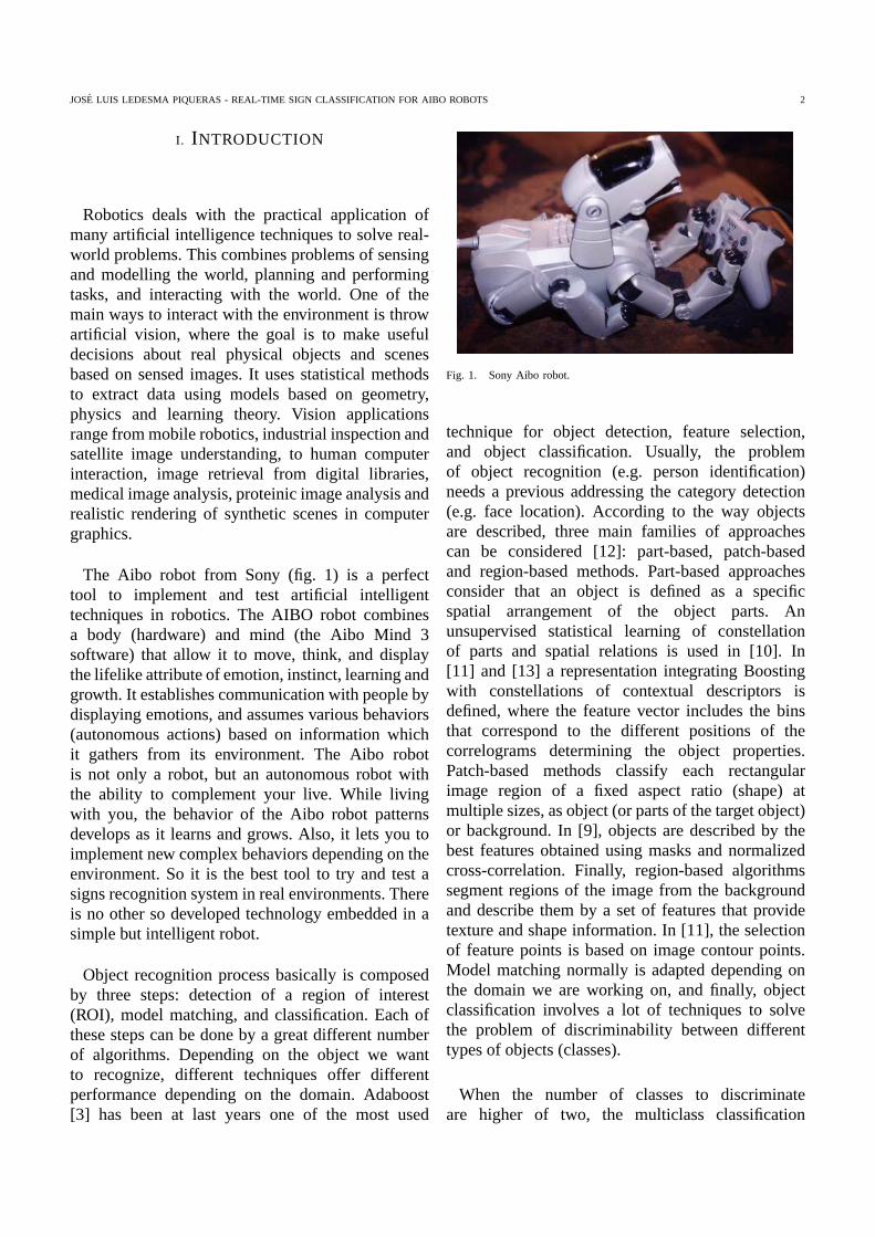
The Aibo robot from Sony (fig. 1) is a perfecttool to implement and test artificial intelligenttechniques in robotics. The AIBO robot combinesa body (hardware) and mind (the Aibo Mind 3software) that allow it to move, think, and displaythe lifelike attribute of emotion, instinct, learning andgrowth. It establishes communication with people bydisplaying emotions, and assumes various behaviors(autonomous actions) based on information whichit gathers from its environment. The Aibo robotis not only a robot, but an autonomous robot withthe ability to complement your live. While livingwith you, the behavior of the Aibo robot patternsdevelops as it learns and grows. Also, it lets you toimplement new complex behaviors depending on theenvironment. So it is the best tool to try and test asigns recognition system in real environments. Thereis no other so developed technology embedded in asimple but intelligent robot.

Object recognition process basically is composedby three steps: detection of a region of interest(ROI), model matching, and classification. Each ofthese steps can be done by a great different numberof algorithms. Depending on the object we wantto recognize, different techniques offer differentperformance depending on the domain. Adaboost[3] has been at last years one of the most used

Fig. 1. Sony Aibo robot.

technique for object detection, feature selection,and object classification. Usually, the problemof object recognition (e.g. person identification)needs a previous addressing the category detection(e.g. face location). According to the way objectsare described, three main families of approachescan be considered [12]: part-based, patch-basedand region-based methods. Part-based approachesconsider that an object is defined as a specificspatial arrangement of the object parts. Anunsupervised statistical learning of constellationof parts and spatial relations is used in [10]. In[11] and [13] a representation integrating Boostingwith constellations of contextual descriptors isdefined, where the feature vector includes the binsthat correspond to the different positions of thecorrelograms determining the object properties.Patch-based methods classify each rectangularimage region of a fixed aspect ratio (shape) atmultiple sizes, as object (or parts of the target object)or background. In [9], objects are described by thebest features obtained using masks and normalizedcross-correlation. Finally, region-based algorithmssegment regions of the image from the backgroundand describe them by a set of features that providetexture and shape information. In [11], the selectionof feature points is based on image contour points.Model matching normally is adapted depending onthe domain we are working on, and finally, objectclassification involves a lot of techniques to solvethe problem of discriminability between differenttypes of objects (classes).

When the number of classes to discriminateare higher of two, the multiclass classification

JOSE LUIS LEDESMA PIQUERAS - REAL-TIME SIGN CLASSIFICATION FOR AIBO ROBOTS 3

is normally generated expending a set of two-class classifiers. The most common classifiersused in the literature are: K-Nearest neighbors,Principal Components Analysis, Fisher DiscriminantAnalysis, Tangent Distance, Adaboost variants,Support Vector Machine, etc.

In our application, we make use of the results of theAdaboost procedure as a detection algorithm. Theuse of this algorithm let us detect regions of interestwith high probability of containing signs. Once theAdaboost returns a ROI, we fit the model using thecircular geometry properties, obtaining the estimatedcenter and the radius of the sign. The main reasonof using the circular geometry is the robustness ofthe algorithm. Once we have fit the model, usingk-NN classification method we obtain the label ofthe sign. We can use safely k-NN with the syntheticsigns we have created, because these signs are verydifferent between them. The system is validatedin a Sony Aibo robot showing good performanceon recognizing objects in real-time. In the nextpart the methodology to solve a real traffic signrecognition system is shown. All the algorithms usedare separately explained. Following one can readabout the results of applying the different algorithms.

This paper is organized as follows: Section 1overviews robotics, artificial vision and introducesthe paper goal and scope. Section 2 describes therequired techniques of the methodology and it showsthe architecture of our proposed system. Section 3shows the experiments and results, and section 4concludes the paper.

II. METHODOLOGY

In this chapter, we explain the techniques usedto solve the model matching and classification ofobjects. Finally, we show the integrated strategies inthe real application.

A. Adabost DetectionThe AdaBoost boosting algorithm has become over

the last few years a very popular algorithm to usein practice. The main idea of AdaBoost is to assigneach example of the given training set a weight. Atthe beginning all weights are equal, but in every

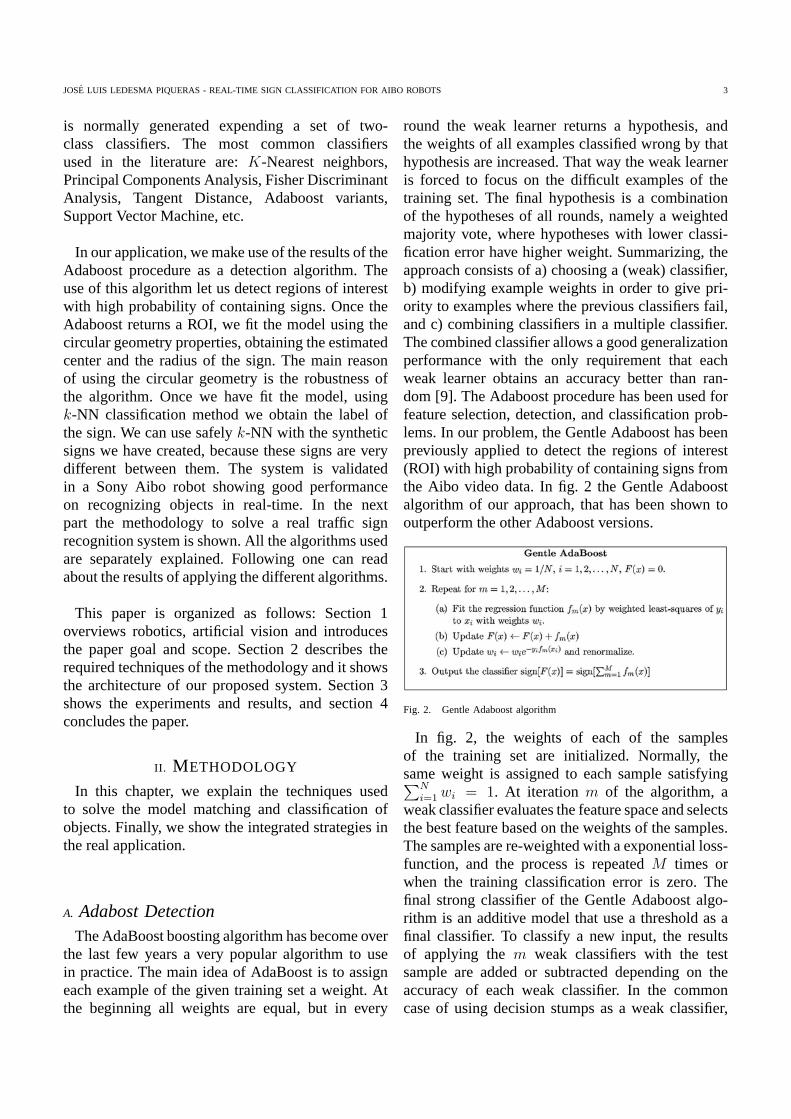
round the weak learner returns a hypothesis, andthe weights of all examples classified wrong by thathypothesis are increased. That way the weak learneris forced to focus on the difficult examples of thetraining set. The final hypothesis is a combinationof the hypotheses of all rounds, namely a weightedmajority vote, where hypotheses with lower classi-fication error have higher weight. Summarizing, theapproach consists of a) choosing a (weak) classifier,b) modifying example weights in order to give pri-ority to examples where the previous classifiers fail,and c) combining classifiers in a multiple classifier.The combined classifier allows a good generalizationperformance with the only requirement that eachweak learner obtains an accuracy better than ran-dom [9]. The Adaboost procedure has been used forfeature selection, detection, and classification prob-lems. In our problem, the Gentle Adaboost has beenpreviously applied to detect the regions of interest(ROI) with high probability of containing signs fromthe Aibo video data. In fig. 2 the Gentle Adaboostalgorithm of our approach, that has been shown tooutperform the other Adaboost versions.

Fig. 2. Gentle Adaboost algorithm

In fig. 2, the weights of each of the samplesof the training set are initialized. Normally, thesame weight is assigned to each sample satisfying∑N

i=1 wi = 1. At iteration m of the algorithm, aweak classifier evaluates the feature space and selectsthe best feature based on the weights of the samples.The samples are re-weighted with a exponential loss-function, and the process is repeated M times orwhen the training classification error is zero. Thefinal strong classifier of the Gentle Adaboost algo-rithm is an additive model that use a threshold as afinal classifier. To classify a new input, the resultsof applying the m weak classifiers with the testsample are added or subtracted depending on theaccuracy of each weak classifier. In the commoncase of using decision stumps as a weak classifier,

JOSE LUIS LEDESMA PIQUERAS - REAL-TIME SIGN CLASSIFICATION FOR AIBO ROBOTS 4

the additive model assigns the same weight to eachof the hypothesis, so all the features are consideredto have the same importance. The last fact is themain difference between the Gentle Adaboost andthe traditional Adaboost versions.

Given an Adaboost positive sample, it determinesa region of interest (ROI) that contains an object.However, besides the ROI we miss information aboutscale and position, so before applying recognitionwe need to apply a spatial normalization. Concernedwith the correlation of sign distortion, we look foraffine transformations that can perform the spatialnormalization to improve final recognition.

B. Model fitting

In order to capture the model contained in thedetected ROI, we consider the radial properties ofthe circular signs to fit a possible instance and toestimate its center and radius.

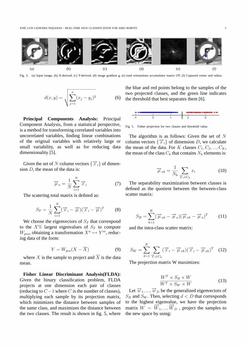
Fast radial symmetry: The fast radial symmetry[4] is calculated over a set of one or more ranges Ndepending on the scale of the features one is trying todetect. The value of the transform at range indicatesthe contribution to radial symmetry of the gradientsa distance n away from each point. At each rangen we define an orientation projection image On (1)and (2), generated by examining the gradient g ateach point p, from which a corresponding positively-affected pixel p+ve(p) and negatively-affected pixelp−ve(p) are determined (3) and (4).

On(P+ve(p)) = On(P+ve(p)) + 1 (1)

On(P−ve(p)) = On(P−ve(p)) + 1 (2)

P+ve(p) = p + roundg(p)

||g(p)||n (3)

P−ve(p) = p − roundg(p)

||g(p)||n (4)

Now, to locate the radial symmetry position, wesearch for the maximum position (x, y) at accumu-lated orientations matrix OT :

OT =n∑

i=1

On (5)

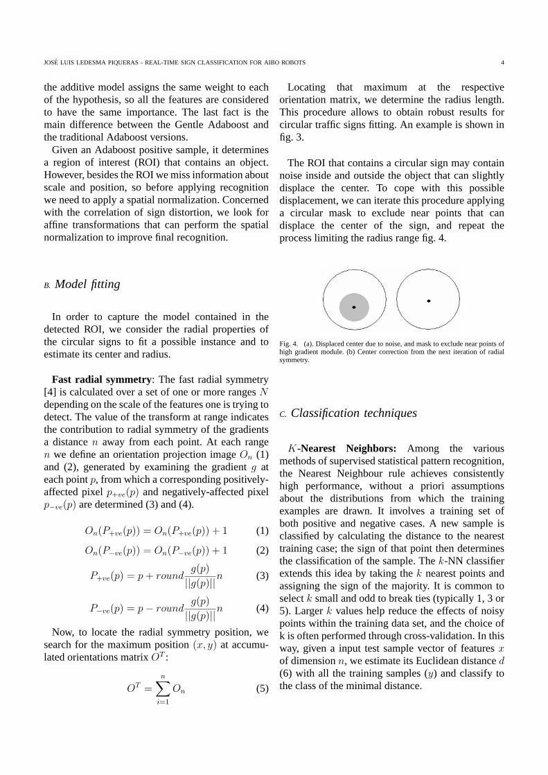
Locating that maximum at the respectiveorientation matrix, we determine the radius length.This procedure allows to obtain robust results forcircular traffic signs fitting. An example is shown infig. 3.

The ROI that contains a circular sign may containnoise inside and outside the object that can slightlydisplace the center. To cope with this possibledisplacement, we can iterate this procedure applyinga circular mask to exclude near points that candisplace the center of the sign, and repeat theprocess limiting the radius range fig. 4.

Fig. 4. (a). Displaced center due to noise, and mask to exclude near points ofhigh gradient module. (b) Center correction from the next iteration of radialsymmetry.

C. Classification techniques

K-Nearest Neighbors: Among the variousmethods of supervised statistical pattern recognition,the Nearest Neighbour rule achieves consistentlyhigh performance, without a priori assumptionsabout the distributions from which the trainingexamples are drawn. It involves a training set ofboth positive and negative cases. A new sample isclassified by calculating the distance to the nearesttraining case; the sign of that point then determinesthe classification of the sample. The k-NN classifierextends this idea by taking the k nearest points andassigning the sign of the majority. It is common toselect k small and odd to break ties (typically 1, 3 or5). Larger k values help reduce the effects of noisypoints within the training data set, and the choice ofk is often performed through cross-validation. In thisway, given a input test sample vector of features xof dimension n, we estimate its Euclidean distance d(6) with all the training samples (y) and classify tothe class of the minimal distance.

JOSE LUIS LEDESMA PIQUERAS - REAL-TIME SIGN CLASSIFICATION FOR AIBO ROBOTS 5

(a) (b) (c) (d) (e) (f)

Fig. 3. (a) Input image, (b) X-derived, (c) Y-derived, (d) image gradient g, (e) total orientations accumulator matrix OT, (f) Captured center and radius.

d(x, y) =

√√√√n∑

j=1

(xj − yj)2 (6)

Principal Components Analysis: PrincipalComponent Analysis, from a statistical perspective,is a method for transforming correlated variables intouncorrelated variables, finding linear combinationsof the original variables with relatively large orsmall variability, as well as for reducing datadimensionality [5].

Given the set of N column vectors {−→x i} of dimen-sion D, the mean of the data is:

−→µ x =1

N

N∑i=1

−→x i (7)

The scatering total matrix is defined as:

ST =1

N

N∑i=1

(−→x i −−→µ )(−→x i −−→µ )T (8)

We choose the eigenvectors of ST that correnpondto the X% largest eigenvalues of ST to computeWpca, obtaining a transformation Xn �→ Y m, reduc-ing data of the form:

Y = Wpca(X − X) (9)

where X is the sample to project and X is the datamean.

Fisher Linear Discriminant Analysis(FLDA):Given the binary classification problem, FLDAprojects at one dimension each pair of classes(reducing to C−1 where C is the number of classes),multiplying each sample by its projection matrix,which minimizes the distance between samples ofthe same class, and maximizes the distance betweenthe two classes. The result is shown in fig. 5, where

the blue and red points belong to the samples of thetwo projected classes, and the green line indicatesthe threshold that best separates them [6].

Fig. 5. Fisher projection for two classes and threshold value.

The algorithm is as follows: Given the set of Ncolumn vectors {−→x i} of dimension D, we calculatethe mean of the data. For K classes C1, C2, ..., CK ,the mean of the class Ck that contains Nk elements is:

−→µ xk =1

Nk

∑−→x i∈Ck

xi (10)

The separability maximization between classes isdefined as the quotient between the between-classscatter matrix:

SB =K∑

k=1

(−→µ xk −−→µ x)(−→µ xk −−→µ x)

T (11)

and the intra-class scatter matrix:

SW =K∑

k=1

∑−→x i∈Ck

(−→x i −−→µ xk)(−→x i −−→µ xk)

T (12)

The projection matrix W maximizes:

W T × SB × W

W T × SW × W(13)

Let −→w 1, ...,−→w D be the generalized eigenvectors of

SB and SW . Then, selecting d < D that correspondsto the highest eigenvalue, we have the projectionmatrix W =

−→W 1, ...,

−→WD , project the samples to

the new space by using:

JOSE LUIS LEDESMA PIQUERAS - REAL-TIME SIGN CLASSIFICATION FOR AIBO ROBOTS 6

−→y = W Td−→x (14)

The generalized eigenvectors of (12) are the eigen-vectors of SBS−1

W .

D. System

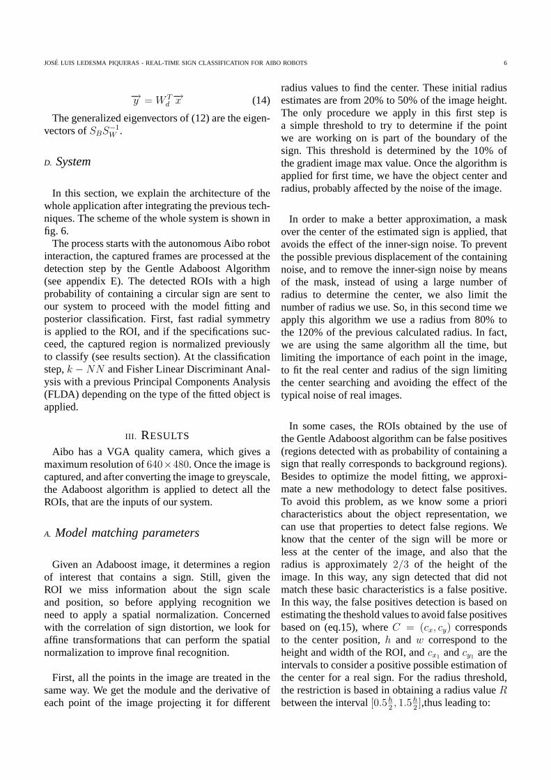
In this section, we explain the architecture of thewhole application after integrating the previous tech-niques. The scheme of the whole system is shown infig. 6.

The process starts with the autonomous Aibo robotinteraction, the captured frames are processed at thedetection step by the Gentle Adaboost Algorithm(see appendix E). The detected ROIs with a highprobability of containing a circular sign are sent toour system to proceed with the model fitting andposterior classification. First, fast radial symmetryis applied to the ROI, and if the specifications suc-ceed, the captured region is normalized previouslyto classify (see results section). At the classificationstep, k − NN and Fisher Linear Discriminant Anal-ysis with a previous Principal Components Analysis(FLDA) depending on the type of the fitted object isapplied.

III. RESULTS

Aibo has a VGA quality camera, which gives amaximum resolution of 640×480. Once the image iscaptured, and after converting the image to greyscale,the Adaboost algorithm is applied to detect all theROIs, that are the inputs of our system.

A. Model matching parameters

Given an Adaboost image, it determines a regionof interest that contains a sign. Still, given theROI we miss information about the sign scaleand position, so before applying recognition weneed to apply a spatial normalization. Concernedwith the correlation of sign distortion, we look foraffine transformations that can perform the spatialnormalization to improve final recognition.

First, all the points in the image are treated in thesame way. We get the module and the derivative ofeach point of the image projecting it for different

radius values to find the center. These initial radiusestimates are from 20% to 50% of the image height.The only procedure we apply in this first step isa simple threshold to try to determine if the pointwe are working on is part of the boundary of thesign. This threshold is determined by the 10% ofthe gradient image max value. Once the algorithm isapplied for first time, we have the object center andradius, probably affected by the noise of the image.

In order to make a better approximation, a maskover the center of the estimated sign is applied, thatavoids the effect of the inner-sign noise. To preventthe possible previous displacement of the containingnoise, and to remove the inner-sign noise by meansof the mask, instead of using a large number ofradius to determine the center, we also limit thenumber of radius we use. So, in this second time weapply this algorithm we use a radius from 80% tothe 120% of the previous calculated radius. In fact,we are using the same algorithm all the time, butlimiting the importance of each point in the image,to fit the real center and radius of the sign limitingthe center searching and avoiding the effect of thetypical noise of real images.

In some cases, the ROIs obtained by the use ofthe Gentle Adaboost algorithm can be false positives(regions detected with as probability of containing asign that really corresponds to background regions).Besides to optimize the model fitting, we approxi-mate a new methodology to detect false positives.To avoid this problem, as we know some a prioricharacteristics about the object representation, wecan use that properties to detect false regions. Weknow that the center of the sign will be more orless at the center of the image, and also that theradius is approximately 2/3 of the height of theimage. In this way, any sign detected that did notmatch these basic characteristics is a false positive.In this way, the false positives detection is based onestimating the theshold values to avoid false positivesbased on (eq.15), where C = (cx, cy) correspondsto the center position, h and w correspond to theheight and width of the ROI, and cx1 and cy1 are theintervals to consider a positive possible estimation ofthe center for a real sign. For the radius threshold,the restriction is based in obtaining a radius value Rbetween the interval [0.5h

2, 1.5h

2],thus leading to:

JOSE LUIS LEDESMA PIQUERAS - REAL-TIME SIGN CLASSIFICATION FOR AIBO ROBOTS 7

Fig. 6. Whole intelligent Aibo process scheme.

cy1 ∈ [0.6h

2, 1.4

h

2], cx1 ∈ [0.6

x

2, 1.4

x

2] (15)

Once we have a good approximation about thecenter and the radius of the circular sign, we haveto normalize it before classification.

B. Normalization parameters

The normalization process consists in four steps.First we rescale it to a 30 × 30 pixels image. Sec-ondly we equalize the image. When one wishes tocompare two or more images on a specific basis,such as texture, it is common to first normalize theirhistograms to a ”standard” histogram. This can beespecially useful when the images have been ac-quired under different circumstances. The most com-mon histogram normalization technique is histogramequalization where one attempts to change the his-togram through the use of a function b = f(a) intoa histogram that is constant for all brightness values.This would correspond to a brightness distributionwhere all values are equally probable. Unfortunately,for an arbitrary image, one can only approximatethis result. For a ”suitable” function f(∗) the relationbetween the input probability density function, theoutput probability density function, and the functionf(∗) is given by:

pb(b)db = pa(a)da =⇒ df =pa(a)da

pb(d)(16)

From (16) we see that ”suitable” means that f(∗)is differentiable and that df/da � 0. For histogramequalization we desire that pb(b) = constant andthis means that:

f(a) = (2B − 1) × p(a) (17)

where P (a) is the probability distribution function.In other words, the quantized probability distributionfunction normalized from 0 to 2B − 1 is the look-up table required for histogram equalization. Thehistogram equalization procedure can also be appliedon a regional basis.

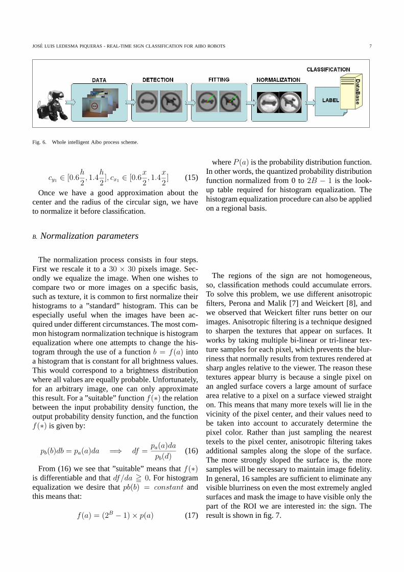
The regions of the sign are not homogeneous,so, classification methods could accumulate errors.To solve this problem, we use different anisotropicfilters, Perona and Malik [7] and Weickert [8], andwe observed that Weickert filter runs better on ourimages. Anisotropic filtering is a technique designedto sharpen the textures that appear on surfaces. Itworks by taking multiple bi-linear or tri-linear tex-ture samples for each pixel, which prevents the blur-riness that normally results from textures rendered atsharp angles relative to the viewer. The reason thesetextures appear blurry is because a single pixel onan angled surface covers a large amount of surfacearea relative to a pixel on a surface viewed straighton. This means that many more texels will lie in thevicinity of the pixel center, and their values need tobe taken into account to accurately determine thepixel color. Rather than just sampling the nearesttexels to the pixel center, anisotropic filtering takesadditional samples along the slope of the surface.The more strongly sloped the surface is, the moresamples will be necessary to maintain image fidelity.In general, 16 samples are sufficient to eliminate anyvisible blurriness on even the most extremely angledsurfaces and mask the image to have visible only thepart of the ROI we are interested in: the sign. Theresult is shown in fig. 7.

JOSE LUIS LEDESMA PIQUERAS - REAL-TIME SIGN CLASSIFICATION FOR AIBO ROBOTS 8

(a) (b)

Fig. 7. (a) Extracted equalized sign. (b) Anisotropic Weickert filter.

C. Database generation

The database we have used is based on over 500images of each class, generated and stored using theprevious procedures. Much more images will lead toa slower system performance, and less images willreduce the percentage of success. In the k-NN appli-cation, a k = 3 has obtained a good performanceas the number of nearest neighbors considered toclassify a given object. The three-class Aibo problemrepresentant are shown in fig. 8.

Fig. 8. Aibo circular classes.

D. Classification parameters

Now that we have the image normalized, theclassification algorithm (k-NN) has to deal with a3-class to return the sign label.

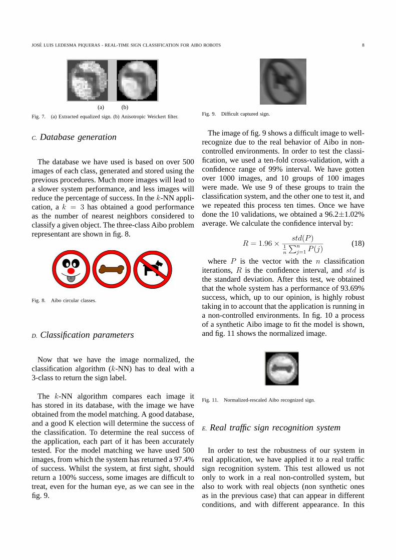
The k-NN algorithm compares each image ithas stored in its database, with the image we haveobtained from the model matching. A good database,and a good K election will determine the success ofthe classification. To determine the real success ofthe application, each part of it has been accuratelytested. For the model matching we have used 500images, from which the system has returned a 97.4%of success. Whilst the system, at first sight, shouldreturn a 100% success, some images are difficult totreat, even for the human eye, as we can see in thefig. 9.

Fig. 9. Difficult captured sign.

The image of fig. 9 shows a difficult image to well-recognize due to the real behavior of Aibo in non-controlled environments. In order to test the classi-fication, we used a ten-fold cross-validation, with aconfidence range of 99% interval. We have gottenover 1000 images, and 10 groups of 100 imageswere made. We use 9 of these groups to train theclassification system, and the other one to test it, andwe repeated this process ten times. Once we havedone the 10 validations, we obtained a 96.2±1.02%average. We calculate the confidence interval by:

R = 1.96 × std(P )1n

∑nj=1 P (j)

(18)

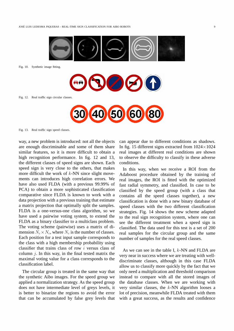
where P is the vector with the n classificationiterations, R is the confidence interval, and std isthe standard deviation. After this test, we obtainedthat the whole system has a performance of 93.69%success, which, up to our opinion, is highly robusttaking in to account that the application is running ina non-controlled environments. In fig. 10 a processof a synthetic Aibo image to fit the model is shown,and fig. 11 shows the normalized image.

Fig. 11. Normalized-rescaled Aibo recognized sign.

E. Real traffic sign recognition system

In order to test the robustness of our system inreal application, we have applied it to a real trafficsign recognition system. This test allowed us notonly to work in a real non-controlled system, butalso to work with real objects (non synthetic onesas in the previous case) that can appear in differentconditions, and with different appearance. In this

JOSE LUIS LEDESMA PIQUERAS - REAL-TIME SIGN CLASSIFICATION FOR AIBO ROBOTS 9

Fig. 10. Synthetic image fitting.

Fig. 12. Real traffic sign circular classes.

Fig. 13. Real traffic sign speed classes.

way, a new problem is introduced: not all the objectsare enough discriminable and some of them sharesimilar features, so it is more difficult to obtain ahigh recognition performance. In fig. 12 and 13,the different classes of speed signs are shown. Eachspeed sign is very close to the others, that makesmore difficult the work of k-NN since slight move-ments can introduces high correlation errors. Wehave also used FLDA (with a previous 99.99% ofPCA) to obtain a more sophisticated classificationcomparative since FLDA is known to work with adata projection with a previous training that estimatea matrix projection that optimally split the samples.FLDA is a one-versus-one class algorithm, so wehave used a pairwise voting system, to extend theFLDA as a binary classifier to a multiclass problem.The voting scheme (pairwise) uses a matrix of di-mension Nc×Nc, where Nc is the number of classes.Each position for a test input sample corresponds tothe class with a high membership probability usingclassifier that trains class of row i versus class ofcolumn j. In this way, in the final tested matrix themaximal voting value for a class corresponds to theclassification label.

The circular group is treated in the same way thatthe synthetic Aibo images. For the speed group weapplied a normalization strategy. As the speed groupdoes not have intermediate level of greys levels, itis better to binarize the regions to avoid the errorthat can be accumulated by false grey levels that

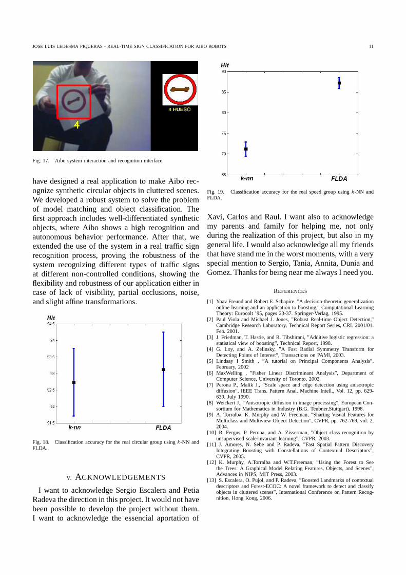
can appear due to different conditions as shadows.In fig. 15 different signs extracted from 1024×1024real images at different real conditions are shownto observe the difficulty to classify in these adverseconditions.

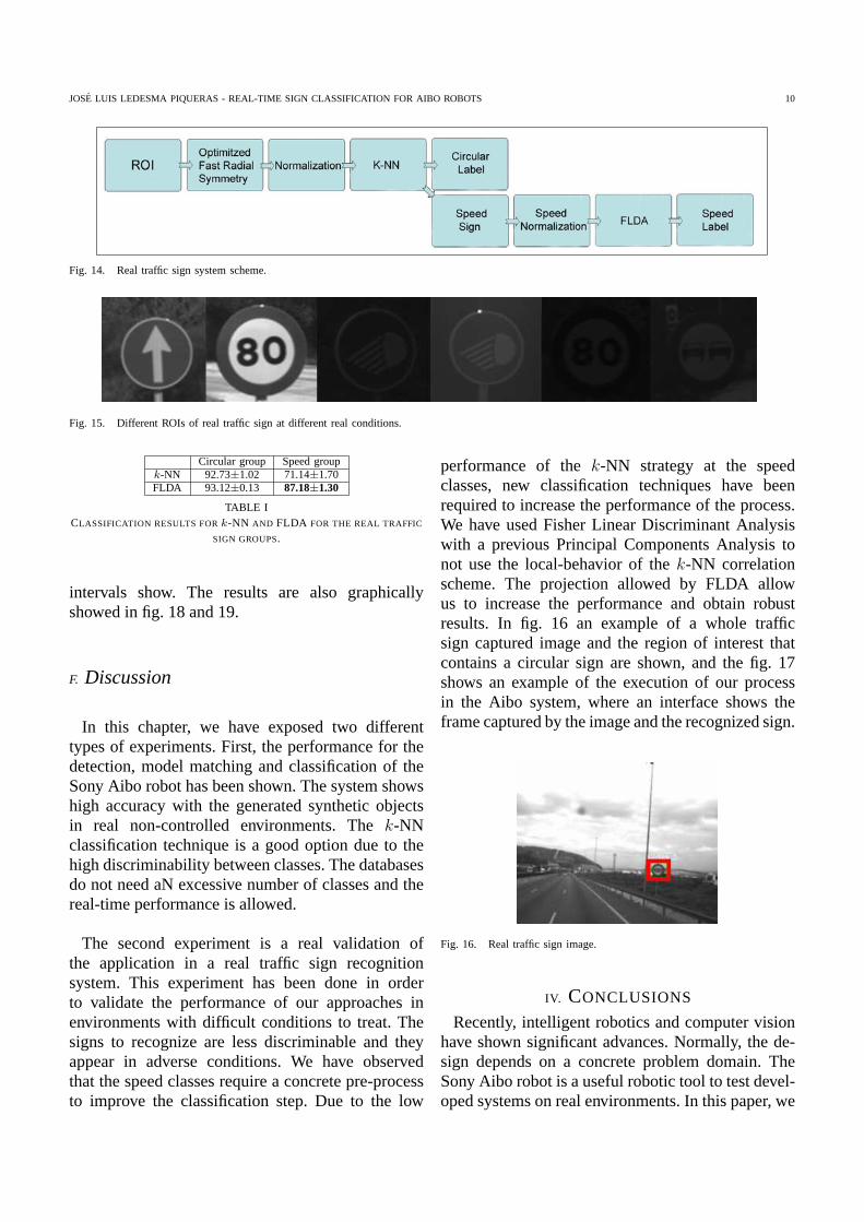
In this way, when we receive a ROI from theAdaboost procedure obtained by the training ofreal images, the ROI is fitted with the optimizedfast radial symmetry, and classified. In case to beclassified by the speed group (with a class thatcontains all the speed classes together), a newclassification is done with a new binary database ofspeed classes with the two different classificationstrategies. Fig. 14 shows the new scheme adaptedto the real sign recognition system, where one cansee the different treatment when a speed sign isclassified. The data used for this test is a set of 200real samples for the circular group and the samenumber of samples for the real speed classes.

As we can see in the table I, k-NN and FLDA arevery near in success where we are treating with well-discriminate classes, although in this case FLDAallow us to classify more quickly by the fact that weonly need a multiplication and threshold comparisoninstead to compare with all the stored images ofthe database classes. When we are working withvery similar classes, the k-NN algorithm looses alot of precision, meanwhile FLDA treated with themwith a great success, as the results and confidence

JOSE LUIS LEDESMA PIQUERAS - REAL-TIME SIGN CLASSIFICATION FOR AIBO ROBOTS 10

Fig. 14. Real traffic sign system scheme.

Fig. 15. Different ROIs of real traffic sign at different real conditions.

Circular group Speed groupk-NN 92.73±1.02 71.14±1.70FLDA 93.12±0.13 87.18±1.30

TABLE ICLASSIFICATION RESULTS FOR k-NN AND FLDA FOR THE REAL TRAFFIC

SIGN GROUPS.

intervals show. The results are also graphicallyshowed in fig. 18 and 19.

F. Discussion

In this chapter, we have exposed two differenttypes of experiments. First, the performance for thedetection, model matching and classification of theSony Aibo robot has been shown. The system showshigh accuracy with the generated synthetic objectsin real non-controlled environments. The k-NNclassification technique is a good option due to thehigh discriminability between classes. The databasesdo not need aN excessive number of classes and thereal-time performance is allowed.

The second experiment is a real validation ofthe application in a real traffic sign recognitionsystem. This experiment has been done in orderto validate the performance of our approaches inenvironments with difficult conditions to treat. Thesigns to recognize are less discriminable and theyappear in adverse conditions. We have observedthat the speed classes require a concrete pre-processto improve the classification step. Due to the low

performance of the k-NN strategy at the speedclasses, new classification techniques have beenrequired to increase the performance of the process.We have used Fisher Linear Discriminant Analysiswith a previous Principal Components Analysis tonot use the local-behavior of the k-NN correlationscheme. The projection allowed by FLDA allowus to increase the performance and obtain robustresults. In fig. 16 an example of a whole trafficsign captured image and the region of interest thatcontains a circular sign are shown, and the fig. 17shows an example of the execution of our processin the Aibo system, where an interface shows theframe captured by the image and the recognized sign.

Fig. 16. Real traffic sign image.

IV. CONCLUSIONS

Recently, intelligent robotics and computer visionhave shown significant advances. Normally, the de-sign depends on a concrete problem domain. TheSony Aibo robot is a useful robotic tool to test devel-oped systems on real environments. In this paper, we

JOSE LUIS LEDESMA PIQUERAS - REAL-TIME SIGN CLASSIFICATION FOR AIBO ROBOTS 11

Fig. 17. Aibo system interaction and recognition interface.

have designed a real application to make Aibo rec-ognize synthetic circular objects in cluttered scenes.We developed a robust system to solve the problemof model matching and object classification. Thefirst approach includes well-differentiated syntheticobjects, where Aibo shows a high recognition andautonomous behavior performance. After that, weextended the use of the system in a real traffic signrecognition process, proving the robustness of thesystem recognizing different types of traffic signsat different non-controlled conditions, showing theflexibility and robustness of our application either incase of lack of visibility, partial occlusions, noise,and slight affine transformations.

Fig. 18. Classification accuracy for the real circular group using k-NN andFLDA.

V. ACKNOWLEDGEMENTS

I want to acknowledge Sergio Escalera and PetiaRadeva the direction in this project. It would not havebeen possible to develop the project without them.I want to acknowledge the essencial aportation of

Fig. 19. Classification accuracy for the real speed group using k-NN andFLDA.

Xavi, Carlos and Raul. I want also to acknowledgemy parents and family for helping me, not onlyduring the realization of this project, but also in mygeneral life. I would also acknowledge all my friendsthat have stand me in the worst moments, with a veryspecial mention to Sergio, Tania, Annita, Dunia andGomez. Thanks for being near me always I need you.

REFERENCES

[1] Yoav Freund and Robert E. Schapire. ”A decision-theoretic generalizationonline learning and an application to boosting,” Computational LearningTheory: Eurocolt ’95, pages 23-37. Springer-Verlag, 1995.

[2] Paul Viola and Michael J. Jones, ”Robust Real-time Object Detection,”Cambridge Research Laboratory, Technical Report Series, CRL 2001/01.Feb. 2001.

[3] J. Friedman, T. Hastie, and R. Tibshirani, ”Additive logistic regression: astatistical view of boosting”, Technical Report, 1998.

[4] G. Loy, and A. Zelinsky, ”A Fast Radial Symmetry Transform forDetecting Points of Interest”, Transactions on PAMI, 2003.

[5] Lindsay I Smith , ”A tutorial on Principal Components Analysis”,February, 2002

[6] MaxWelling , ”Fisher Linear Discriminant Analysis”, Department ofComputer Science, University of Toronto, 2002.

[7] Perona P., Malik J., ”Scale space and edge detection using anisotropicdiffusion”, IEEE Trans. Pattern Anal. Machine Intell., Vol. 12, pp. 629-639, July 1990.

[8] Weickert J., ”Anisotropic diffusion in image processing”, European Con-sortium for Mathematics in Industry (B.G. Teubner,Stuttgart), 1998.

[9] A. Torralba, K. Murphy and W. Freeman, ”Sharing Visual Features forMulticlass and Multiview Object Detection”, CVPR, pp. 762-769, vol. 2,2004.

[10] R. Fergus, P. Perona, and A. Zisserman, ”Object class recognition byunsupervised scale-invariant learning”, CVPR, 2003.

[11] J. Amores, N. Sebe and P. Radeva, ”Fast Spatial Pattern DiscoveryIntegrating Boosting with Constellations of Contextual Descriptors”,CVPR, 2005.

[12] K. Murphy, A.Torralba and W.T.Freeman, ”Using the Forest to Seethe Trees: A Graphical Model Relating Features, Objects, and Scenes”,Advances in NIPS, MIT Press, 2003.

[13] S. Escalera, O. Pujol, and P. Radeva, ”Boosted Landmarks of contextualdescriptors and Forest-ECOC: A novel framework to detect and classifyobjects in cluttered scenes”, International Conference on Pattern Recog-nition, Hong Kong, 2006.

Appendices

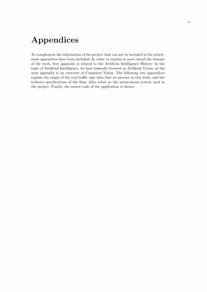
To complement the information of the project that can not be included in the article,some appendices have been included. In order to explain in more detail the domainof the work, first appendix is related to the Artificial Intelligence History. In thetopic of Artificial Intelligence, we have basically focused on Artificial Vision, so thenext appendix is an overview of Computer Vision. The following two appendicesexplain the origin of the real traffic sign data that we process in this work, and thetechnics specifications of the Sony Aibo robot as the autonomous system used inthe project. Finally, the source code of the application is shown.

24

12

Appendix A. Artificial IntelligencehistoryPrehistory of AI

Humans have always speculated about the nature of mind, thought, and language,and searched for discrete representations of their knowledge. Aristotle tried to for-malize this speculation by means of syllogistic logic, which remains one of the keystrategies of AI. The first is-a hierarchy was created in 260 by Porphyry of Tyros.Classical and medieval grammarians explored more subtle features of language thatAristotle shortchanged, and mathematician Bernard Bolzano made the first modernattempt to formalize semantics in 1837.

Early computer design was driven mainly by the complex mathematics needed totarget weapons accurately, with analog feedback devices inspiring an ideal of cyber-netics. The expression ”artificial intelligence” was introduced as a ’digital’ replace-ment for the analog ’cybernetics’.

Development of AI theory

Much of the (original) focus of artificial intelligence research draws from an ex-perimental approach to psychology, and emphasizes what may be called linguisticintelligence (best exemplified in the Turing test).

Approaches to Artificial Intelligence that do not focus on linguistic intelligence in-clude robotics and collective intelligence approaches, which focus on active manipu-lation of an environment, or consensus decision making, and draw from biology andpolitical science when seeking models of how ”intelligent” behavior is organized.

AI also draws from animal studies, in particular with insects, which are easier toemulate as robots (see artificial life), as well as animals with more complex cogni-tion, including apes, who resemble humans in many ways but have less developedcapacities for planning and cognition. Some researchers argue that animals, whichare apparently simpler than humans, ought to be considerably easier to mimic. Butsatisfactory computational models for animal intelligence are not available.

Seminal papers advancing AI include ”A Logical Calculus of the Ideas Immanent inNervous Activity” (1943), by Warren McCulloch and Walter Pitts, and ”On Com-puting Machinery and Intelligence” (1950), by Alan Turing, and ”Man-ComputerSymbiosis” by J.C.R. Licklider. See Cybernetics and Turing test for further discus-sion.

There were also early papers which denied the possibility of machine intelligence onlogical or philosophical grounds such as ”Minds, Machines and Godel” (1961) byJohn Lucas.

With the development of practical techniques based on AI research, advocates of

10

13

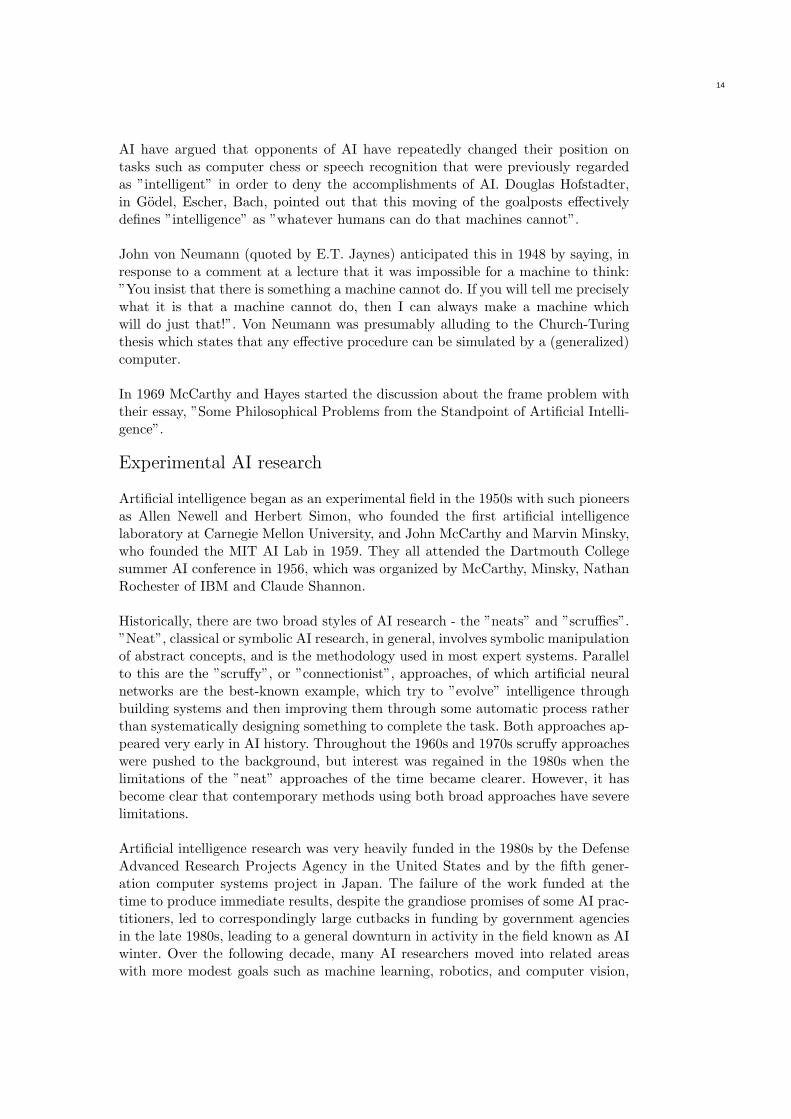
AI have argued that opponents of AI have repeatedly changed their position ontasks such as computer chess or speech recognition that were previously regardedas ”intelligent” in order to deny the accomplishments of AI. Douglas Hofstadter,in Godel, Escher, Bach, pointed out that this moving of the goalposts effectivelydefines ”intelligence” as ”whatever humans can do that machines cannot”.

John von Neumann (quoted by E.T. Jaynes) anticipated this in 1948 by saying, inresponse to a comment at a lecture that it was impossible for a machine to think:”You insist that there is something a machine cannot do. If you will tell me preciselywhat it is that a machine cannot do, then I can always make a machine whichwill do just that!”. Von Neumann was presumably alluding to the Church-Turingthesis which states that any effective procedure can be simulated by a (generalized)computer.

In 1969 McCarthy and Hayes started the discussion about the frame problem withtheir essay, ”Some Philosophical Problems from the Standpoint of Artificial Intelli-gence”.

Experimental AI research

Artificial intelligence began as an experimental field in the 1950s with such pioneersas Allen Newell and Herbert Simon, who founded the first artificial intelligencelaboratory at Carnegie Mellon University, and John McCarthy and Marvin Minsky,who founded the MIT AI Lab in 1959. They all attended the Dartmouth Collegesummer AI conference in 1956, which was organized by McCarthy, Minsky, NathanRochester of IBM and Claude Shannon.

Historically, there are two broad styles of AI research - the ”neats” and ”scruffies”.”Neat”, classical or symbolic AI research, in general, involves symbolic manipulationof abstract concepts, and is the methodology used in most expert systems. Parallelto this are the ”scruffy”, or ”connectionist”, approaches, of which artificial neuralnetworks are the best-known example, which try to ”evolve” intelligence throughbuilding systems and then improving them through some automatic process ratherthan systematically designing something to complete the task. Both approaches ap-peared very early in AI history. Throughout the 1960s and 1970s scruffy approacheswere pushed to the background, but interest was regained in the 1980s when thelimitations of the ”neat” approaches of the time became clearer. However, it hasbecome clear that contemporary methods using both broad approaches have severelimitations.

Artificial intelligence research was very heavily funded in the 1980s by the DefenseAdvanced Research Projects Agency in the United States and by the fifth gener-ation computer systems project in Japan. The failure of the work funded at thetime to produce immediate results, despite the grandiose promises of some AI prac-titioners, led to correspondingly large cutbacks in funding by government agenciesin the late 1980s, leading to a general downturn in activity in the field known as AIwinter. Over the following decade, many AI researchers moved into related areaswith more modest goals such as machine learning, robotics, and computer vision,

11

14

though research in pure AI continued at reduced levels.

Micro-World AI

The real world is full of distracting and obscuring detail: generally science progressesby focusing on artificially simple models of reality (in physics, frictionless planes andperfectly rigid bodies, for example). In 1970 Marvin Minsky and Seymour Papert,of the MIT AI Laboratory, proposed that AI research should likewise focus ondeveloping programs capable of intelligent behaviour in artificially simple situationsknown as micro-worlds. Much research has focused on the so-called blocks world,which consists of coloured blocks of various shapes and sizes arrayed on a flat surface.Micro-World AI

Spinoffs

Whilst progress towards the ultimate goal of human-like intelligence has been slow,many spinoffs have come in the process. Notable examples include the languagesLISP and Prolog, which were invented for AI research but are now used for non-AItasks. Hacker culture first sprang from AI laboratories, in particular the MIT AILab, home at various times to such luminaries as John McCarthy, Marvin Minsky,Seymour Papert (who developed Logo there) and Terry Winograd (who abandonedAI after developing SHRDLU).

AI languages and programming styles

AI research has led to many advances in programming languages including the firstlist processing language by Allen Newell et. al., Lisp dialects, Planner, Actors, theScientific Community Metaphor, production systems, and rule-based languages.

GOFAI TEST research is often done in programming languages such as Prologor Lisp. Bayesian work often uses Matlab or Lush (a numerical dialect of Lisp).These languages include many specialist probabilistic libraries. Real-life and espe-cially real-time systems are likely to use C++. AI programmers are often academicsand emphasise rapid development and prototyping rather than bulletproof softwareengineering practices, hence the use of interpreted languages to empower rapidcommand-line testing and experimentation.

The most basic AI program is a single If-Then statement, such as ”If A, then B.”If you type an ’A’ letter, the computer will show you a ’B’ letter. Basically, you areteaching a computer to do a task. You input one thing, and the computer respondswith something you told it to do or say. All programs have If-Then logic. A morecomplex example is if you type in ”Hello.”, and the computer responds ”How areyou today?” This response is not the computer’s own thought, but rather a line youwrote into the program before. Whenever you type in ”Hello.”, the computer alwaysresponds ”How are you today?”. It seems as if the computer is alive and thinkingto the casual observer, but actually it is an automated response. AI is often a longseries of If-Then (or Cause and Effect) statements.

12

15

A randomizer can be added to this. The randomizer creates two or more responsepaths. For example, if you type ”Hello”, the computer may respond with ”Howare you today?” or ”Nice weather” or ”Would you like to play a game?” Threeresponses (or ’thens’) are now possible instead of one. There is an equal chancethat any one of the three responses will show. This is similar to a pull-cord talkingdoll that can respond with a number of sayings. A computer AI program can havethousands of responses to the same input. This makes it less predictable and closer tohow a real person would respond, arguably because living people respond somewhatunpredictably. When thousands of input (”if”) are written in (not just ”Hello.”) andthousands of responses (”then”) are written into the AI program, then the computercan talk (or type) with most people, if those people know the If statement inputlines to type.

Many games, like chess and strategy games, use action responses instead of typedresponses, so that players can play against the computer. Robots with AI brainswould use If-Then statements and randomizers to make decisions and speak. How-ever, the input may be a sensed object in front of the robot instead of a ”Hello.”line, and the response may be to pick up the object instead of a response line.

Chronological History

Historical Antecedents

Greek myths of Hephaestus and Pygmalion incorporate the idea of intelligent robots.In the 5th century BC, Aristotle invented syllogistic logic, the first formal deductivereasoning system.

Ramon Llull, Spanish theologian, invented paper ”machines” for discovering non-mathematical truths through combinattions of words from lists in the 13th century.

By the 15th century and 16th century, clocks, the first modern measuring machines,were first produced using lathes. Clockmakers extended their craft to creating me-chanical animals and other novelties. Rabbi Judah Loew ben Bezalel of Prague issaid to have invented the Golem, a clay man brought to life (1580).

Early in the 17th century, Rene Descartes proposed that bodies of animals arenothing more than complex machines. Many other 17th century thinkers offeredvariations and elaborations of Cartesian mechanism. Thomas Hobbes publishedLeviathan, containing a material and combinatorial theory of thinking. Blaise Pascalcreated the second mechanical and first digital calculating machine (1642). GottfriedLeibniz improved Pascal’s machine, making the Stepped Reckoner to do multiplica-tion and division (1673) and evisioned a universal calculus of reasoning (Alphabetof human thought) by which arguments could be decided mechanically.

The 18th century saw a profusion of mechanical toys, including the celebrated me-chanical duck of Jacques de Vaucanson and Wolfgang von Kempelen’s phony chess-playing automaton, The Turk (1769).

13

16

Mary Shelley published the story of Frankenstein; or the Modern Prometheus (1818).

19th and Early 20th Century

George Boole developed a binary algebra (Boolean algebra) representing (some)”laws of thought.” Charles Babbage and Ada Lovelace worked on programmablemechanical calculating machines.

In the first years of the 20th century Bertrand Russell and Alfred North White-head published Principia Mathematica, which revolutionized formal logic. Russell,Ludwig Wittgenstein, and Rudolf Carnap lead philosophy into logical analysis ofknowledge. Karel Capek’s play R.U.R. (Rossum’s Universal Robots)) opens in Lon-don (1923). This is the first use of the word ”robot” in English.

Mid 20th century and Early AI

Warren Sturgis McCulloch and Walter Pitts publish ”A Logical Calculus of theIdeas Immanent in Nervous Activity” (1943), laying foundations for artificial neuralnetworks. Arturo Rosenblueth, Norbert Wiener and Julian Bigelow coin the term”cybernetics” in a 1943 paper. Wiener’s popular book by that name published in1948. Vannevar Bush published As We May Think (The Atlantic Monthly, July1945) a prescient vision of the future in which computers assist humans in manyactivities.

The man widely acknowledged as the father of computer science, Alan Turing, pub-lished ”Computing Machinery and Intelligence” (1950) which introduced the Turingtest as a way of operationalizing a test of intelligent behavior. Claude Shannon pub-lished a detailed analysis of chess playing as search (1950). Isaac Asimov publishedhis Three Laws of Robotics (1950).

1956: John McCarthy coined the term ”artificial intelligence” as the topic of theDartmouth Conference, the first conference devoted to the subject.

Demonstration of the first running AI program, the Logic Theorist (LT) written byAllen Newell, J.C. Shaw and Herbert Simon (Carnegie Institute of Technology, nowCarnegie Mellon University).

1957: The General Problem Solver (GPS) demonstrated by Newell, Shaw and Simon.

1952-1962: Arthur Samuel (IBM) wrote the first game-playing program, for checkers(draughts), to achieve sufficient skill to challenge a world champion. Samuel’s ma-chine learning programs were responsible for the high performance of the checkersplayer.

1958: John McCarthy (Massachusetts Institute of Technology or MIT) inventedthe Lisp programming language. Herb Gelernter and Nathan Rochester (IBM) de-scribed a theorem prover in geometry that exploits a semantic model of the domainin the form of diagrams of ”typical” cases. Teddington Conference on the Mecha-nization of Thought Processes was held in the UK and among the papers presented

14

17

were John McCarthy’s Programs with Common Sense, Oliver Selfridge’s Pandemo-nium, and Marvin Minsky’s Some Methods of Heuristic Programming and ArtificialIntelligence.

Late 1950s and early 1960s: Margaret Masterman and colleagues at University ofCambridge design semantic nets for machine translation.

1961: James Slagle (PhD dissertation, MIT) wrote (in Lisp) the first symbolic in-tegration program, SAINT, which solved calculus problems at the college freshmanlevel.

1962: First industrial robot company, Unimation, founded.

1963: Thomas Evans’ program, ANALOGY, written as part of his PhD work atMIT, demonstrated that computers can solve the same analogy problems as aregiven on IQ tests. Edward Feigenbaum and Julian Feldman published Computersand Thought, the first collection of articles about artificial intelligence.

1964: Danny Bobrow’s dissertation at MIT (technical report #1 from MIT’s AIgroup, Project MAC), shows that computers can understand natural language wellenough to solve algebra word problems correctly. Bert Raphael’s MIT dissertationon the SIR program demonstrates the power of a logical representation of knowledgefor question-answering systems.

1965: J. Alan Robinson invented a mechanical proof procedure, the ResolutionMethod, which allowed programs to work efficiently with formal logic as a rep-resentation language. Joseph Weizenbaum (MIT) built ELIZA (program), an inter-active program that carries on a dialogue in English language on any topic. It wasa popular toy at AI centers on the ARPANET when a version that ”simulated” thedialogue of a psychotherapist was programmed.

1966: Ross Quillian (PhD dissertation, Carnegie Inst. of Technology, now CMU)demonstrated semantic nets. First Machine Intelligence workshop at Edinburgh: thefirst of an influential annual series organized by Donald Michie and others. Negativereport on machine translation kills much work in Natural language processing (NLP)for many years.

1967: Dendral program (Edward Feigenbaum, Joshua Lederberg, Bruce Buchanan,Georgia Sutherland at Stanford University) demonstrated to interpret mass spec-tra on organic chemical compounds. First successful knowledge-based program forscientific reasoning. Joel Moses (PhD work at MIT) demonstrated the power ofsymbolic reasoning for integration problems in the Macsyma program. First suc-cessful knowledge-based program in mathematics. Richard Greenblatt (program-mer) at MIT built a knowledge-based chess-playing program, MacHack, that wasgood enough to achieve a class-C rating in tournament play.

1968: Marvin Minsky and Seymour Papert publish Perceptrons, demonstrating lim-its of simple neural nets.

15

18

1969: Stanford Research Institute (SRI): Shakey the Robot, demonstrated combin-ing animal locomotion, perception and problem solving. Roger Schank (Stanford)defined conceptual dependency model for natural language understanding. Laterdeveloped (in PhD dissertations at Yale University) for use in story understandingby Robert Wilensky and Wendy Lehnert, and for use in understanding memory byJanet Kolodner. Yorick Wilks (Stanford) developed the semantic coherence view oflanguage called Preference Semantics, embodied in the first semantics-driven ma-chine translation program, and the basis of many PhD dissertations since such asBran Boguraev and David Carter at Cambridge. First International Joint Confer-ence on Artificial Intelligence (IJCAI) held at Stanford.

1970: Jaime Carbonell (Sr.) developed SCHOLAR, an interactive program for com-puter assisted instruction based on semantic nets as the representation of knowledge.Bill Woods described Augmented Transition Networks (ATN’s) as a representationfor natural language understanding. Patrick Winston’s PhD program, ARCH, atMIT learned concepts from examples in the world of children’s blocks.

Early 70’s: Jane Robinson and Don Walker established an influential Natural Lan-guage Processing group at SRI.

1971: Terry Winograd’s PhD thesis (MIT) demonstrated the ability of computers tounderstand English sentences in a restricted world of children’s blocks, in a couplingof his language understanding program, SHRDLU, with a robot arm that carriedout instructions typed in English.

1972: Prolog programming language developed by Alain Colmerauer.

1973: The Assembly Robotics Group at University of Edinburgh builds FreddyRobot, capable of using visual perception to locate and assemble models. TheLighthill report gives a largely negative verdict on AI research in Great Britainand forms the basis for the decision by the British government to discontine sup-port for AI research in all but two universities.

1974: Ted Shortliffe’s PhD dissertation on the MYCIN program (Stanford) demon-strated the power of rule-based systems for knowledge representation and inferencein the domain of medical diagnosis and therapy. Sometimes called the first expertsystem. Earl Sacerdoti developed one of the first planning programs, ABSTRIPS,and developed techniques of hierarchical planning.

1975: Marvin Minsky published his widely-read and influential article on Frames as arepresentation of knowledge, in which many ideas about schemas and semantic linksare brought together. The Meta-Dendral learning program produced new results inchemistry (some rules of mass spectrometry) the first scientific discoveries by acomputer to be published in a referreed journal.

Mid 70’s: Barbara Grosz (SRI) established limits to traditional AI approaches todiscourse modeling. Subsequent work by Grosz, Bonnie Webber and Candace Sidnerdeveloped the notion of ”centering”, used in establishing focus of discourse and

16

19

anaphoric references in NLP. David Marr and MIT colleagues describe the ”primalsketch” and its role in visual perception.

1976: Douglas Lenat’s AM program (Stanford PhD dissertation) demonstrated thediscovery model (loosely-guided search for interesting conjectures). Randall Davisdemonstrated the power of meta-level reasoning in his PhD dissertation at Stanford.

Late 70’s: Stanford’s SUMEX-AIM resource, headed by Ed Feigenbaum and JoshuaLederberg, demonstrates the power of the ARPAnet for scientific collaboration.

1978: Tom Mitchell, at Stanford, invented the concept of Version Spaces for describ-ing the search space of a concept formation program. Herbert Simon wins the NobelPrize in Economics for his theory of bounded rationality, one of the cornerstones ofAI known as ”satisficing”. The MOLGEN program, written at Stanford by MarkStefik and Peter Friedland, demonstrated that an object-oriented programming rep-resentation of knowledge can be used to plan gene-cloning experiments.

1979: Bill VanMelle’s PhD dissertation at Stanford demonstrated the generalityof MYCIN’s representation of knowledge and style of reasoning in his EMYCINprogram, the model for many commercial expert system ”shells”. Jack Myers andHarry Pople at University of Pittsburgh developed INTERNIST, a knowledge-basedmedical diagnosis program based on Dr. Myers’ clinical knowledge. Cordell Green,David Barstow, Elaine Kant and others at Stanford demonstrated the CHI systemfor automatic programming. The Stanford Cart, built by Hans Moravec, becomesthe first computer-controlled, autonomous vehicle when it successfully traverses achair-filled room and circumnavigates the Stanford AI Lab. Drew McDermott andJon Doyle at MIT, and John McCarthy at Stanford begin publishing work on non-monotonic logics and formal aspects of truth maintenance.

1980s: Lisp machines developed and marketed. First expert system shells and com-mercial applications.

1980: Lee Erman, Rick Hayes-Roth, Victor Lesser and Raj Reddy published the firstdescription of the blackboard model, as the framework for the HEARSAY-II speechunderstanding system. First National Conference of the American Association forArtificial Intelligence (AAAI) held at Stanford.

1981: Danny Hillis designs the connection machine, a massively parallel architecturethat brings new power to AI, and to computation in general. (Later founds ThinkingMachines, Inc.)

1982: The Fifth Generation Computer Systems project (FGCS), an initiative byJapan’s Ministry of International Trade and Industry, begun in 1982, to create a”fifth generation computer” (see history of computing hardware) which was sup-posed to perform much calculation utilizing massive parallelism.

1983: John Laird and Paul Rosenbloom, working with Allen Newell, complete CMUdissertations on Soar (program). James F. Allen invents the Interval Calculus, the

17

20

first widely used formalization of temporal events.

Mid 80’s: Neural Networks become widely used with the Backpropagation algorithm(first described by Paul Werbos in 1974).

1985: The autonomous drawing program, AARON, created by Harold Cohen, isdemonstrated at the AAAI National Conference (based on more than a decade ofwork, and with subsequent work showing major developments).

1987: Marvin Minsky publishes The Society of Mind, a theoretical description ofthe mind as a collection of cooperating agents.

1989: Dean Pomerleau at CMU creates ALVINN (An Autonomous Land Vehiclein a Neural Network), which grew into the system that drove a car coast-to-coastunder computer control for all but about 50 of the 2850 miles.

1990s: Major advances in all areas of AI, with significant demonstrations in machinelearning, intelligent tutoring, case-based reasoning, multi-agent planning, schedul-ing, uncertain reasoning, data mining, natural language understanding and trans-lation, vision, virtual reality, games, and other topics. Rodney Brooks’ MIT Cogproject, with numerous collaborators, makes significant progress in building a hu-manoid robot.

Early 90’s: TD-Gammon, a backgammon program written by Gerry Tesauro, demon-strates that reinforcement (learning) is powerful enough to create a championship-level game-playing program by competing favorably with world-class players.

1997: The Deep Blue chess program (IBM) beats the world chess champion, GarryKasparov, in a widely followed match. First official RoboCup football (soccer) matchfeaturing table-top matches with 40 teams of interacting robots and over 5000 spec-tators.

1998: Tim Berners-Lee published his Semantic Web Road map paper [2].

Late 90’s: Web crawlers and other AI-based information extraction programs be-come essential in widespread use of the World Wide Web. Demonstration of anIntelligent room and Emotional Agents at MIT’s AI Lab. Initiation of work onthe Oxygen architecture, which connects mobile and stationary computers in anadaptive network.

2000: Interactive robopets (”smart toys”) become commercially available, realizingthe vision of the 18th century novelty toy makers. Cynthia Breazeal at MIT pub-lishes her dissertation on Sociable machines, describing Kismet (robot), with a facethat expresses emotions. The Nomad robot explores remote regions of Antarcticalooking for meteorite samples.

2004: OWL Web Ontology Language W3C Recommendation (10 February 2004).

18

21

Appendix B. Computer VisionThe field of computer vision can be characterized as immature and diverse. Eventhough earlier work exists, it was not until the late 1970’s that a more focused studyof the field started when computers could manage the processing of large data setssuch as images. However, these studies usually originated from various other fields,and consequently there is no standard formulation of the ”computer vision prob-lem”. Also, and to an even larger extent, there is no standard formulation of howcomputer vision problems should be solved. Instead, there exists an abundance ofmethods for solving various well-defined computer vision tasks, where the methodsoften are very task specific and seldom can be generalized over a wide range ofapplications. Many of the methods and applications are still in the state of basicresearch, but more and more methods have found their way into commercial prod-ucts, where they often constitute a part of a larger system which can solve complextasks (e.g., in the area of medical images, or quality control and measurements inindustrial processes).

Computer vision is by some seen as a subfield of artificial intelligence where imagedata is being fed into a system as an alternative to text based input for controllingthe behaviour of a system. Some of the learning methods which are used in computervision are based on learning techniques developed within artificial intelligence.

Since a camera can be seen as a light sensor, there are various methods in computervision based on correspondences between a physical phenomenon related to lightand images of that phenomenon. For example, it is possible to extract informationabout motion in fluids and about waves by analyzing images of these phenomena.Also, a subfield within computer vision deals with the physical process which givena scene of objects, light sources, and camera lenses forms the image in a camera.Consequently, computer vision can also be seen as an extension of physics.

A third field which plays an important role is neurobiology, specifically the study ofthe biological vision system. Over the last century, there has been an extensive studyof eyes, neurons, and the brain structures devoted to processing of visual stimuliin both humans and various animals. This has led to a coarse, yet complicated,description of how ”real” vision systems operate in order to solve certain visionrelated tasks. These results have led to a subfield within computer vision whereartificial systems are designed to mimic the processing and behaviour of biologicalsystems, at different levels of complexity. Also, some of the learning-based methodsdeveloped within computer vision have their background in biology.

Yet another field related to computer vision is signal processing. Many existingmethods for processing of one-variable signals, typically temporal signals, can beextended in a natural way to processing of two-variable signals or multi-variablesignals in computer vision. However, because of the specific nature of images thereare many methods developed within computer vision which have no counterpart inthe processing of one-variable signals. A distinct character of these methods is thefact that they are non-linear which, together with the multi-dimensionality of the

19

22

signal, defines a subfield in signal processing as a part of computer vision.

Beside the above mentioned views on computer vision, many of the related researchtopics can also be studied from a purely mathematical point of view. For example,many methods in computer vision are based on statistics, optimization or geometry.Finally, a significant part of the field is devoted to the implementation aspect ofcomputer vision; how existing methods can be realized in various combinations ofsoftware and hardware, or how these methods can be modified in order to gainprocessing speed without losing too much performance.

Related fields

Computer vision, Image processing, Image analysis, Robot vision and Machine vi-sion are closely related fields. If you look inside text books which have either ofthese names in the title there is a significant overlap in terms of what techniquesand applications they cover. This implies that the basic techniques that are usedand developed in these fields are more or less identical, something which can beinterpreted as there is only one field with different names.

On the other hand, it appears to be necessary for research groups, scientific journals,conferences and companies to present or market themselves as belonging specificallyto one of these fields and, hence, various characterizations which distinguish eachof the fields from the others have been presented. The following characterizationsappear relevant but should not be taken as universally accepted.

Image processing and Image analysis tend to focus on 2D images, how to transformone image to another, e.g., by pixel-wise operations such as contrast enhancement,local operations such as edge extraction or noise removal, or geometrical transfor-mations such as rotating the image. This characterization implies that image pro-cessing/analysis does not produce nor require assumptions about what a specificimage is an image of.

Computer vision tends to focus on the 3D scene projected onto one or several images,e.g., how to reconstruct structure or other information about the 3D scene from oneor several images. Computer vision often relies on more or less complex assumptionsabout the scene depicted in an image.

Machine vision tends to focus on applications, mainly in industry, e.g., vision basedautonomous robots and systems for vision based inspection or measurement. Thisimplies that image sensor technologies and control theory often are integrated withthe processing of image data to control a robot and that real-time processing isemphasized by means of efficient implementations in hardware and software.

There is also a field called Imaging which primarily focus on the process of produc-ing images, but sometimes also deals with processing and analysis of images. Forexample, Medical imaging contains lots of work on the analysis of image data inmedical applications.

20

23

Finally, pattern recognition is a field which uses various methods to extract infor-mation from signals in general, mainly based on statistical approaches. A significantpart of this field is devoted to applying these methods to image data.

A consequence of this state of affairs is that you can be working in a lab related toone of these fields, apply methods from a second field to solve a problem in a thirdfield and present the result at a conference related to a fourth field!

Examples of applications for computer vision

Another way to describe computer vision is in terms of applications areas. Oneof the most prominent application fields is medical computer vision or medicalimage processing. This area is characterized by the extraction of information fromimage data for the purpose of making a medical diagnosis of a patient. Typicallyimage data is in the form of microscopy images, X-ray images, angiography images,ultrasonic images, and tomography images. An example of information which canbe extracted from such image data is detection of tumours, arteriosclerosis or othermalign changes. It can also be measurements of organ dimensions, blood flow, etc.This application area also supports medical research by providing new information,e.g., about the structure of the brain, or about the quality of medical treatments.

A second application area in computer vision is in industry. Here, information isextracted for the purpose of supporting a manufacturing process. One example isquality control where details or final products are being automatically inspected inorder to find defects. Another example is measurement of position and orientationof details to be picked up by a robot arm. See the article on machine vision for moredetails on this area.

Military applications are probably one of the largest areas for computer vision,even though only a small part of this work is open to the public. The obviousexamples are detection of enemy soldiers or vehicles and guidance of missiles to adesignated target. More advanced systems for missile guidance send the missile toan area rather than a specific target, and target selection is made when the missilereaches the area based on locally acquired image data. Modern military concepts,such as ”battlefield awareness,” imply that various sensors, including image sensors,provide a rich set of information about a combat scene which can be used to supportstrategic decisions. In this case, automatic processing of the data is used to reducecomplexity and to fuse information from multiple sensors to increase reliability.

One of the newer application areas is autonomous vehicles, which include sub-mersibles, land-based vehicles (small robots with wheels, cars or trucks), and aerialvehicles. An unmanned aerial vehicle is often denoted UAV. The level of auton-omy ranges from fully autonomous (unmanned) vehicles to vehicles where com-puter vision based systems support a driver or a pilot in various situations. Fullyautonomous vehicles typically use computer vision for navigation, i.e. for knowingwhere it is, or for producing a map of its environment (SLAM) and for detectingobstacles. It can also be used for detecting certain task specific events, e. g., a UAVlooking for forest fires. Examples of supporting system are obstacle warning systems

21

24

in cars and systems for autonomous landing of aircraft. Several car manufacturershave demonstrated systems for autonomous driving of cars, but this technology hasstill not reached a level where it can be put on the market. There are ample exam-ples of military autonomous vehicles ranging from advanced missiles to UAVs forrecon missions or missile guidance. Space exploration is already being made withautonomous vehicles using computer vision, e. g., NASA’s Mars Exploration Rover.

Other application areas include the creation of visual effects for cinema and broad-cast, e.g., camera tracking or matchmoving, and surveillance.

Typical tasks of computer vision

Object recognition

Detecting the presence of known objects or living beings in an image, possiblytogether with estimating the pose of these objects.

Examples: Searching in digital images for specific content (content-based imageretrieval) Recognizing human faces and their location in images. Estimation of thethree-dimensional pose of humans and their limbs Detection of objects which arepassing through a manufacturing process, e.g., on a conveyor belt, and estimationof their pose so that a robot arm can pick up the objects from the belt.

Optical character recognition

OCR (optical character recognition) takes pictures of printed or handwritten textand converts it into computer readable text such as ASCII or Unicode. In the pastimages were acquired with a computer scanner, however more recently some softwarecan also read text from pictures taken with a digital camera.

Tracking

Tracking known objects through an image sequence.

Examples: Tracking a single person walking through a shopping center. Tracking ofvehicles moving along a road.

Scene interpretation

Creating a model from an image/video.

Examples: Creating a model of the surrounding terrain from images, which arebeing taken by a robot-mounted camera. Anticipating the pattern of the image todetermine size and density to estimate the volume using tomography like device.The cloud recognition is one the government project using this method.

Egomotion

The goal of egomotion computation is to describe the motion of an object with

22

25

respect to an external reference system, by analyzing data acquired by sensors on-board on the object. i.e. the camera itself.

Examples: Given two images of a scene, determine the 3d rigid motion of the camerabetween the two views.

Computer vision systems

A typical computer vision system can be divided in the following subsystems:

Image acquisition

The image or image sequence is acquired with an imaging system (camera, radar,lidar, tomography system). Often the imaging system has to be calibrated beforebeing used.

Preprocessing

In the preprocessing step, the image is being treated with ”low-level”-operations.The aim of this step is to do noise reduction on the image (i.e. to dissociate thesignal from the noise) and to reduce the overall amount of data. This is typicallybeing done by employing different (digital)image processing methods such as: Down-sampling the image. Applying digital filters convolutions, computing a scale spacerepresentation Correlations or linear shift invariant filters Sobel operator Comput-ing the x- and y-gradient (possibly also the time-gradient). Segmenting the image.Pixelwise thresholding. Performing an eigentransform on the image Fourier trans-form Doing motion estimation for local regions of the image (also known as opticalflow estimation). Estimating disparity in stereo images. Multiresolution analysis

Feature extraction

The aim of feature extraction is to further reduce the data to a set of features,which ought to be invariant to disturbances such as lighting conditions, cameraposition, noise and distortion. Examples of feature extraction are: Performing edgedetection or estimation of local orientation. Extracting corner features. Detectingblob features. Extracting spin images from depth maps. Extracting geons or otherthree-dimensional primitives, such as superquadrics. Acquiring contour lines andmaybe curvature zero crossings. Generating features with the Scale-invariant featuretransform.

Registration

The aim of the registration step is to establish correspondence between the featuresin the acquired set and the features of known objects in a model-database and/orthe features of the preceding image. The registration step has to bring up a finalhypothesis. To name a few methods: Least squares estimation Hough transform inmany variations Geometric hashing Particle filtering RANdom SAmple Consensus.

23

26

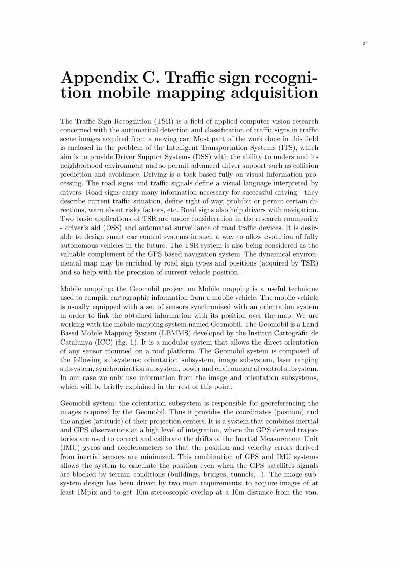
Appendix C. Traffic sign recogni-tion mobile mapping adquisition

The Traffic Sign Recognition (TSR) is a field of applied computer vision researchconcerned with the automatical detection and classification of traffic signs in trafficscene images acquired from a moving car. Most part of the work done in this fieldis enclosed in the problem of the Intelligent Transportation Systems (ITS), whichaim is to provide Driver Support Systems (DSS) with the ability to understand itsneighborhood environment and so permit advanced driver support such as collisionprediction and avoidance. Driving is a task based fully on visual information pro-cessing. The road signs and traffic signals define a visual language interpreted bydrivers. Road signs carry many information necessary for successful driving - theydescribe current traffic situation, define right-of-way, prohibit or permit certain di-rections, warn about risky factors, etc. Road signs also help drivers with navigation.Two basic applications of TSR are under consideration in the research community- driver’s aid (DSS) and automated surveillance of road traffic devices. It is desir-able to design smart car control systems in such a way to allow evolution of fullyautonomous vehicles in the future. The TSR system is also being considered as thevaluable complement of the GPS-based navigation system. The dynamical environ-mental map may be enriched by road sign types and positions (acquired by TSR)and so help with the precision of current vehicle position.

Mobile mapping: the Geomobil project on Mobile mapping is a useful techniqueused to compile cartographic information from a mobile vehicle. The mobile vehicleis usually equipped with a set of sensors synchronized with an orientation systemin order to link the obtained information with its position over the map. We areworking with the mobile mapping system named Geomobil. The Geomobil is a LandBased Mobile Mapping System (LBMMS) developed by the Institut Cartografic deCatalunya (ICC) (fig. 1). It is a modular system that allows the direct orientationof any sensor mounted on a roof platform. The Geomobil system is composed ofthe following subsystems: orientation subsystem, image subsystem, laser rangingsubsystem, synchronization subsystem, power and environmental control subsystem.In our case we only use information from the image and orientation subsystems,which will be briefly explained in the rest of this point.

Geomobil system: the orientation subsystem is responsible for georeferencing theimages acquired by the Geomobil. Thus it provides the coordinates (position) andthe angles (attitude) of their projection centers. It is a system that combines inertialand GPS observations at a high level of integration, where the GPS derived trajec-tories are used to correct and calibrate the drifts of the Inertial Measurement Unit(IMU) gyros and accelerometers so that the position and velocity errors derivedfrom inertial sensors are minimized. This combination of GPS and IMU systemsallows the system to calculate the position even when the GPS satellites signalsare blocked by terrain conditions (buildings, bridges, tunnels,...). The image sub-system design has been driven by two main requirements: to acquire images of atleast 1Mpix and to get 10m stereoscopic overlap at a 10m distance from the van.

3

27

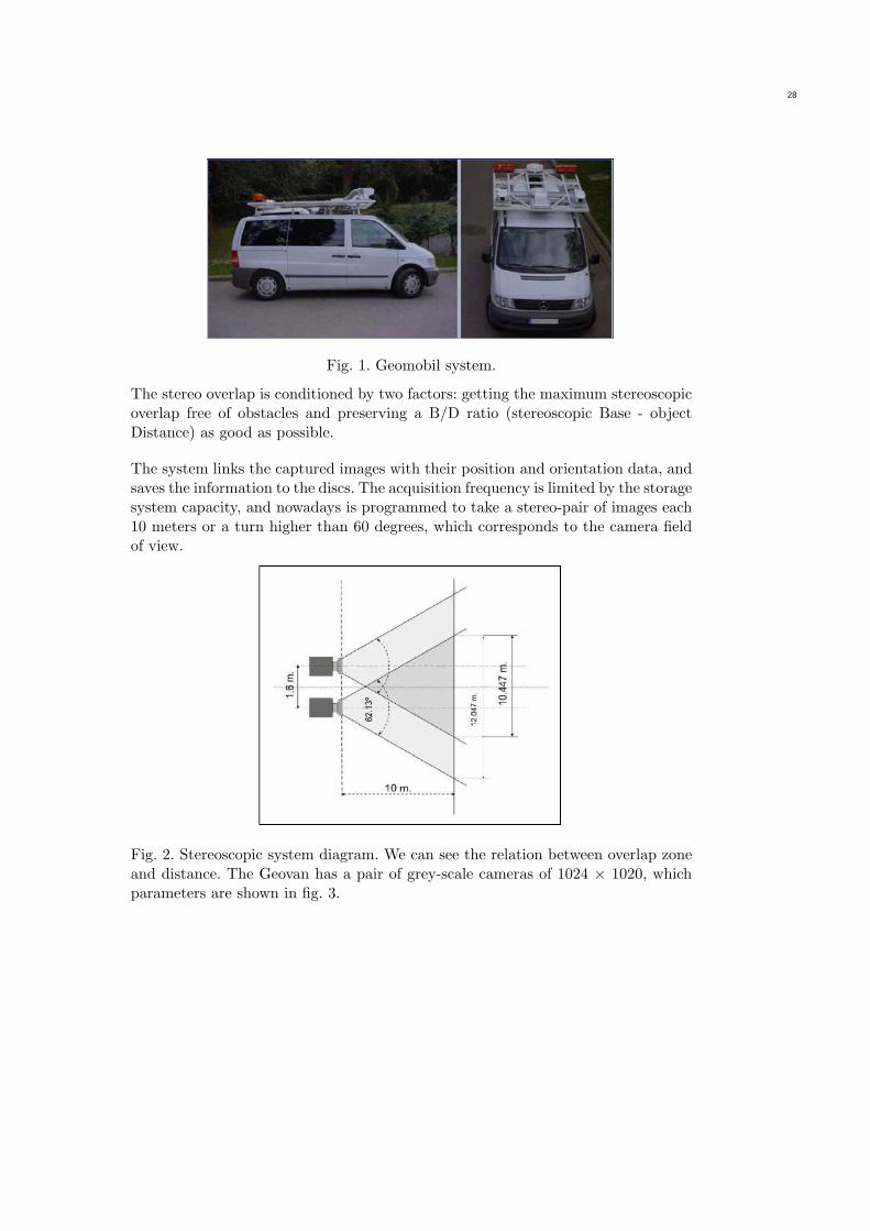
Fig. 1. Geomobil system.

The stereo overlap is conditioned by two factors: getting the maximum stereoscopicoverlap free of obstacles and preserving a B/D ratio (stereoscopic Base - objectDistance) as good as possible.

The system links the captured images with their position and orientation data, andsaves the information to the discs. The acquisition frequency is limited by the storagesystem capacity, and nowadays is programmed to take a stereo-pair of images each10 meters or a turn higher than 60 degrees, which corresponds to the camera fieldof view.

Fig. 2. Stereoscopic system diagram. We can see the relation between overlap zoneand distance. The Geovan has a pair of grey-scale cameras of 1024 × 1020, whichparameters are shown in fig. 3.

4

28

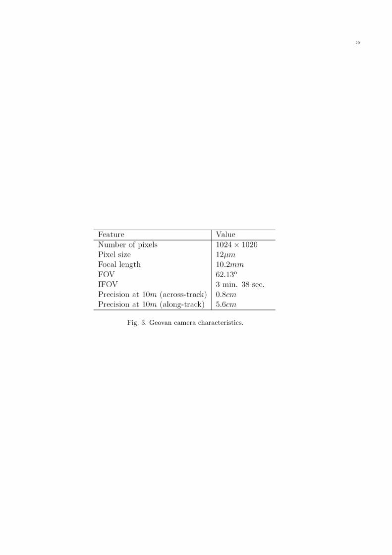
Fig. 3. Geovan camera characteristics.

5

29

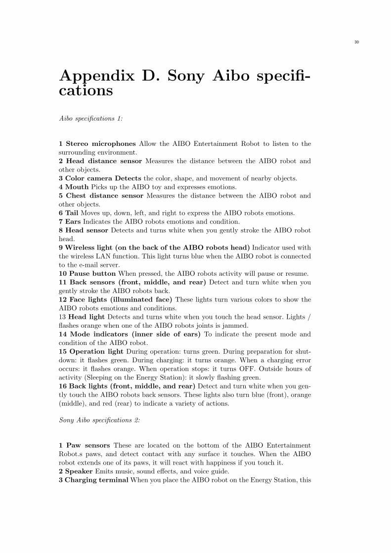
Appendix D. Sony Aibo specifi-cations

Aibo specifications 1:

1 Stereo microphones Allow the AIBO Entertainment Robot to listen to thesurrounding environment.2 Head distance sensor Measures the distance between the AIBO robot andother objects.3 Color camera Detects the color, shape, and movement of nearby objects.4 Mouth Picks up the AIBO toy and expresses emotions.5 Chest distance sensor Measures the distance between the AIBO robot andother objects.6 Tail Moves up, down, left, and right to express the AIBO robots emotions.7 Ears Indicates the AIBO robots emotions and condition.8 Head sensor Detects and turns white when you gently stroke the AIBO robothead.9 Wireless light (on the back of the AIBO robots head) Indicator used withthe wireless LAN function. This light turns blue when the AIBO robot is connectedto the e-mail server.10 Pause button When pressed, the AIBO robots activity will pause or resume.11 Back sensors (front, middle, and rear) Detect and turn white when yougently stroke the AIBO robots back.12 Face lights (illuminated face) These lights turn various colors to show theAIBO robots emotions and conditions.13 Head light Detects and turns white when you touch the head sensor. Lights /flashes orange when one of the AIBO robots joints is jammed.14 Mode indicators (inner side of ears) To indicate the present mode andcondition of the AIBO robot.15 Operation light During operation: turns green. During preparation for shut-down: it flashes green. During charging: it turns orange. When a charging erroroccurs: it flashes orange. When operation stops: it turns OFF. Outside hours ofactivity (Sleeping on the Energy Station): it slowly flashing green.16 Back lights (front, middle, and rear) Detect and turn white when you gen-tly touch the AIBO robots back sensors. These lights also turn blue (front), orange(middle), and red (rear) to indicate a variety of actions.

Sony Aibo specifications 2:

1 Paw sensors These are located on the bottom of the AIBO EntertainmentRobot.s paws, and detect contact with any surface it touches. When the AIBOrobot extends one of its paws, it will react with happiness if you touch it.2 Speaker Emits music, sound effects, and voice guide.3 Charging terminal When you place the AIBO robot on the Energy Station, this

6

30

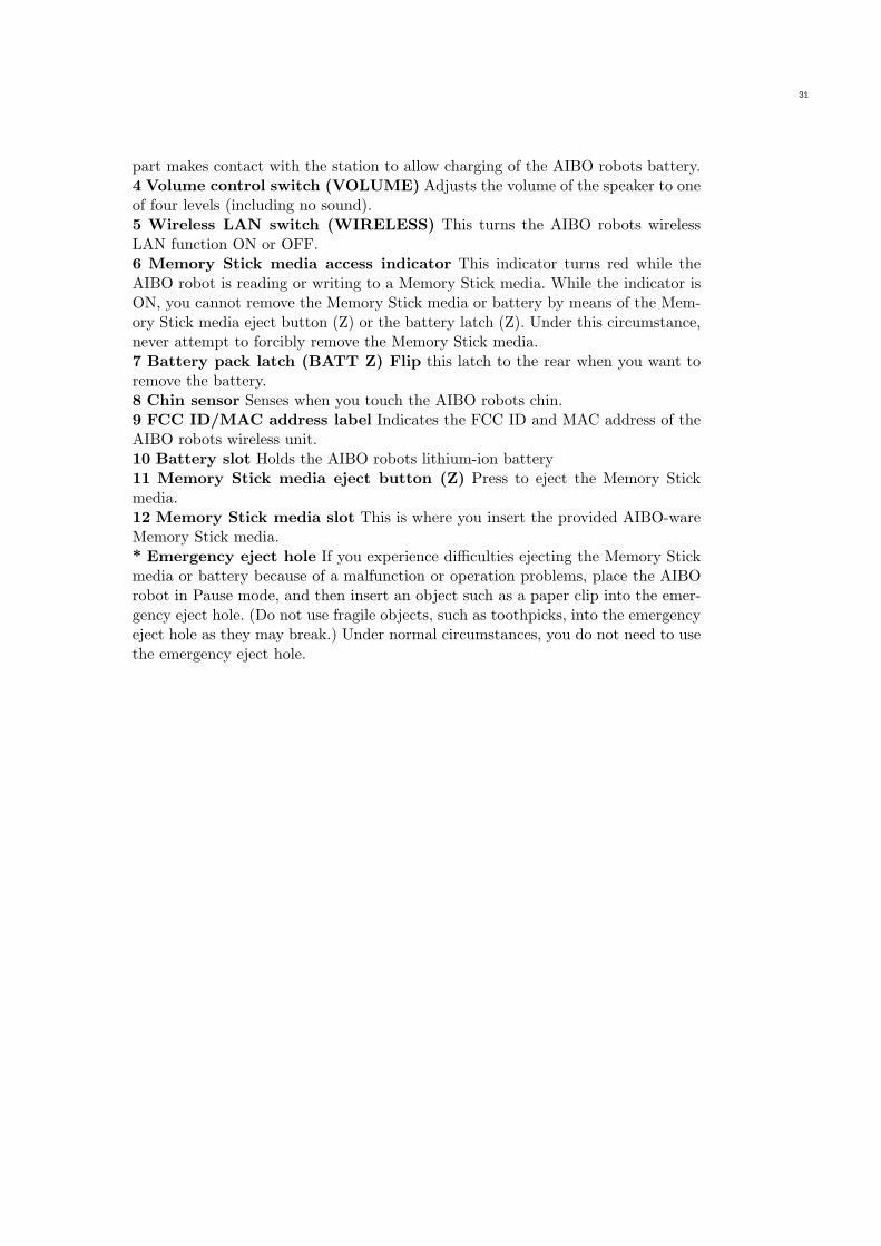
part makes contact with the station to allow charging of the AIBO robots battery.4 Volume control switch (VOLUME) Adjusts the volume of the speaker to oneof four levels (including no sound).5 Wireless LAN switch (WIRELESS) This turns the AIBO robots wirelessLAN function ON or OFF.6 Memory Stick media access indicator This indicator turns red while theAIBO robot is reading or writing to a Memory Stick media. While the indicator isON, you cannot remove the Memory Stick media or battery by means of the Mem-ory Stick media eject button (Z) or the battery latch (Z). Under this circumstance,never attempt to forcibly remove the Memory Stick media.7 Battery pack latch (BATT Z) Flip this latch to the rear when you want toremove the battery.8 Chin sensor Senses when you touch the AIBO robots chin.9 FCC ID/MAC address label Indicates the FCC ID and MAC address of theAIBO robots wireless unit.10 Battery slot Holds the AIBO robots lithium-ion battery11 Memory Stick media eject button (Z) Press to eject the Memory Stickmedia.12 Memory Stick media slot This is where you insert the provided AIBO-wareMemory Stick media.* Emergency eject hole If you experience difficulties ejecting the Memory Stickmedia or battery because of a malfunction or operation problems, place the AIBOrobot in Pause mode, and then insert an object such as a paper clip into the emer-gency eject hole. (Do not use fragile objects, such as toothpicks, into the emergencyeject hole as they may break.) Under normal circumstances, you do not need to usethe emergency eject hole.

7

31

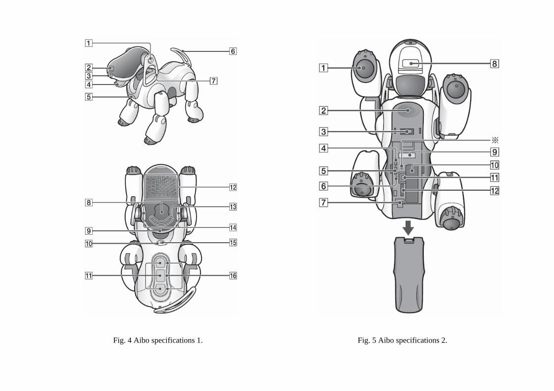
Fig. 4 Aibo specifications 1. Fig. 5 Aibo specifications 2.

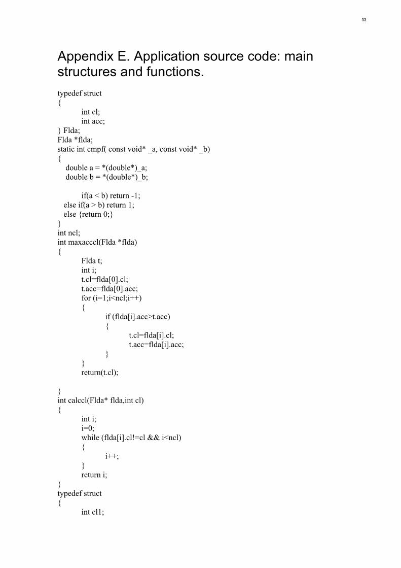
Appendix E. Application source code: main structures and functions.

typedef struct

{

int cl;

int acc;

} Flda;

Flda *flda;

static int cmpf( const void* _a, const void* _b)

{

double a = *(double*)_a;

double b = *(double*)_b;

if(a < b) return -1;

else if(a > b) return 1;

else {return 0;}

}

int ncl;

int maxacccl(Flda *flda)

{

Flda t;

int i;

t.cl=flda[0].cl;

t.acc=flda[0].acc;

for (i=1;i<ncl;i++)

{

if (flda[i].acc>t.acc)

{

t.cl=flda[i].cl;

t.acc=flda[i].acc;

}

}

return(t.cl);

}

int calccl(Flda* flda,int cl)

{

int i;

i=0;

while (flda[i].cl!=cl && i<ncl)

{

i++;

}

return i;

}

typedef struct

{

int cl1;

33

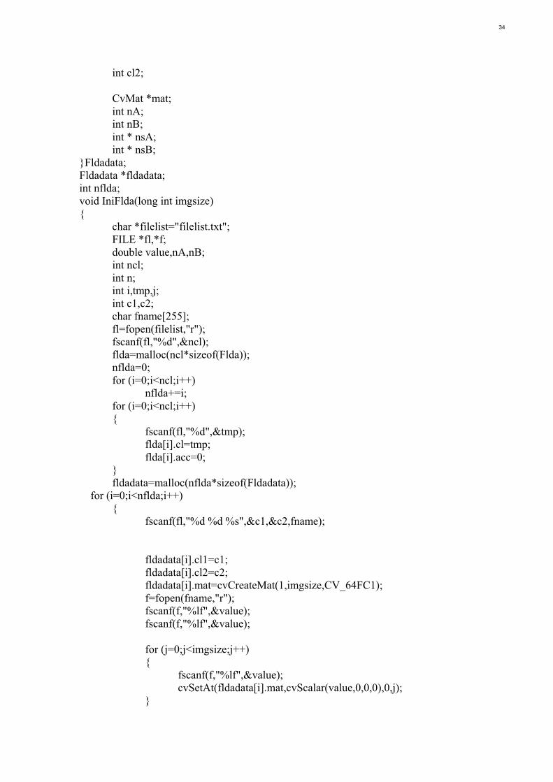
int cl2;

CvMat *mat;

int nA;

int nB;

int * nsA;

int * nsB;

}Fldadata;

Fldadata *fldadata;

int nflda;

void IniFlda(long int imgsize)

{

char *filelist="filelist.txt";

FILE *fl,*f;

double value,nA,nB;

int ncl;

int n;

int i,tmp,j;

int c1,c2;

char fname[255];

fl=fopen(filelist,"r");

fscanf(fl,"%d",&ncl);

flda=malloc(ncl*sizeof(Flda));

nflda=0;

for (i=0;i<ncl;i++)

nflda+=i;

for (i=0;i<ncl;i++)

{

fscanf(fl,"%d",&tmp);

flda[i].cl=tmp;

flda[i].acc=0;

}

fldadata=malloc(nflda*sizeof(Fldadata));

for (i=0;i<nflda;i++)

{

fscanf(fl,"%d %d %s",&c1,&c2,fname);

fldadata[i].cl1=c1;

fldadata[i].cl2=c2;

fldadata[i].mat=cvCreateMat(1,imgsize,CV_64FC1);

f=fopen(fname,"r");

fscanf(f,"%lf",&value);

fscanf(f,"%lf",&value);

for (j=0;j<imgsize;j++)

{

fscanf(f,"%lf",&value);

cvSetAt(fldadata[i].mat,cvScalar(value,0,0,0),0,j);

}

34

fscanf(f,"%lf",&nA);

fscanf(f,"%lf",&nB);

fldadata[i].nA=nA;

fldadata[i].nB=nB;

fldadata[i].nsA=malloc(fldadata[i].nA*sizeof(int));

fldadata[i].nsB=malloc(fldadata[i].nB*sizeof(int));

for (j=0;j<fldadata[i].nA;j++)

{

fscanf(f,"%lf",&value);

fldadata[i].nsA[j]=value;

}

for (j=0;j<fldadata[i].nB;j++)

{

fscanf(f,"%lf",&value);

fldadata[i].nsB[j]=value;

}

fclose(f);

}

fclose(fl);

}

int clasflda(IplImage *img,int kn)

{

char *filelist="filelist.txt";

FILE *fl,*f;

int i,tmp,j;

int c1,c2,ce1,ce2;

double nA,nB;

char fname[100];

char lastname[100];

double value,sum,e1,e2;

int t1,t2;

CvMat *mat,*imgmat,*rimgmat,*rtimgmat;

CvMemStorage* storagetempA;

CvMemStorage* storagetempB;

CvSeq* seqA;

CvSeq* seqB;

storagetempA = cvCreateMemStorage(0);

storagetempB = cvCreateMemStorage(0);

seqA = cvCreateSeq( CV_64FC1, /* sequence of integer elements */

sizeof(CvSeq), /* header size - no extra

fields */

sizeof(double), /* element size */

storagetempA /* the container storage */ );

seqB = cvCreateSeq( CV_64FC1, /* sequence of integer elements */

sizeof(CvSeq), /* header size - no extra fields */

sizeof(double), /* element size */

storagetempB /* the container storage */ );

35

imgmat=cvCreateMatHeader(img->height,img->width,CV_8UC1);

imgmat=cvGetMat(img,imgmat,NULL,0);

rtimgmat=cvCreateMat(img->height,img->width,CV_64FC1);

rimgmat=cvCreateMat(img->height*img->width,1,CV_64FC1);

cvConvertScale(imgmat,rtimgmat,1,0);

cvReshape(rtimgmat,rimgmat,1,1);

for (j=0;j<nflda;j++)

{

sum=cvDotProduct(fldadata[j].mat,rimgmat);

sum=sum/255.0;

for (i=0;i<fldadata[j].nA;i++)

{

value=fldadata[j].nsA[i];

value=value-sum;

value*=(value<0? -1:1);

cvSeqPush(seqA,&value);

}

cvSeqSort(seqA,cmpf,0);

for (i=0;i<fldadata[j].nB;i++)

{

value=fldadata[j].nsB[i];

value=value-sum;

value*=(value<0? -1:1);

cvSeqPush(seqB,&value);

}

cvSeqSort(seqB,cmpf,0);

e1=*(double*)cvGetSeqElem( seqA, 0 );

e2=*(double*)cvGetSeqElem( seqB, 0 );

i=0;

ce1=0;

ce2=0;

c1=calccl(flda,fldadata[j].cl1);

c2=calccl(flda,fldadata[j].cl2);

while (i<kn)

{

if (e1<e2)

{

ce1++;

e1=*(double*)cvGetSeqElem(seqA,ce1);

} else

{

ce2++;

e2=*(double*)cvGetSeqElem(seqB,ce2);

}

i++;

}

if (ce1>ce2)

36

{

flda[c1].acc++;

} else

{

flda[c2].acc++;

}

cvClearSeq(seqA);

cvClearSeq(seqB);

}

return maxacccl(flda);

}

int valid=1;

IplImage *detecta2(IplImage *imgO);

typedef struct Class

{

float dif;

int y;

}

Class;

typedef struct structClass

{

CvRect* rectangulo;

int clase_final;

}

structClass;

static int cmp_func( const void* _a, const void* _b)

{

float* a = (float*)_a;

float* b = (float*)_b;

if(a[4] < b[4]) return 1;

else if(a[4] > b[4]) return -1;

else {if(a[5] < b[5]) return 1;

else if(a[5] > b[5]) return -1;

else return 0;}

}

static int cmp_func2( const void* _a, const void* _b)

{

Class* a = (Class*)_a;

Class* b = (Class*)_b;

37

if(a->dif < b->dif) return -1;

else if(a->dif > b->dif) return 1;

else {return 0;}

}

float angulo( int a, int b)

{

float aux;

float F;

if(a==0){

if(b>0){

F=(float)(CV_PI/2);

}else{ F=(float)((3*CV_PI)/2);}

}else{

if (b==0){

if(a>0) F=0;

else F=(float)CV_PI;

}

else{

aux= (float)atan2(b,a);

if(a>0 && b>0) F=(float)(CV_PI-aux);

if(a<0 && b<0) F=-aux;

if(a>0 && b<0) F=-aux;

if(a<0 && b>0) F=(float)(aux+CV_PI);

}

}

F=(float)((F*360)/(2*CV_PI));

return F;

}

CvPoint interseccion( CvPoint a1 , CvPoint a2 , CvPoint b1 , CvPoint b2)

{

CvPoint tall;

int x_tall;

int y_tall;

float m1=(float) (a2.y - a1.y)/(a2.x - a1.x);

float m2=(float) (b2.y - b1.y)/(b2.x - b1.x);

float c1= a1.y - (m1 * a1.x);

float c2= b1.y - (m2 * b1.x);

x_tall=(int)((c2-c1)/(m1-m2));

y_tall=(int)(m1*x_tall+c1);

38

tall = cvPoint(x_tall,y_tall);

return tall;

}

IplImage* drawSquares( IplImage* imagen, CvSeq* clases )

{

CvFont fuente;

CvPoint pt1,pt2;

CvRect* r;

char texto[2];

structClass* numero;

int i;

//Inicializamos la fuente

cvInitFont(&fuente, CV_FONT_VECTOR0,0.8,0.8,0,2,8);

// Leemos 4 elementos de la secuencia al mismo tiempo(vertices del rectangulo)

for( i = 0; i < clases->total; i ++ )

{

numero = ( structClass* )cvGetSeqElem( clases , i);

r= numero->rectangulo;

pt1.x = r->x;

pt2.x = r->x + r->width;

pt1.y = r->y;

pt2.y = r->y + r->height;

// Pintamos el rectangulo

cvRectangle( imagen, pt1, pt2, CV_RGB(255,0,0), 3, 8, 0);

// Pintamos el texto

printf("%d\n",numero->clase_final);

itoa(numero->clase_final,texto,10);

cvPutText( imagen, texto, cvPoint(pt2.x - (r->width/2),pt2.y + 25),

&fuente, CV_RGB(255,255,0));

}

return imagen;

}

IplImage* transform( IplImage* origen, IplImage* destino,IplImage* mascara ,CvPoint

int1 , CvPoint int2 , CvPoint int3 )

{

39

CvPoint2D32f sp[4];

CvPoint2D32f dp[4];

double m[9];

CvMat map_matrix = cvMat( 3, 3, CV_64F, m );

sp[0] = cvPoint2D32f(int1.x,int1.y);

sp[1] = cvPoint2D32f(int2.x,int2.y);

sp[2] = cvPoint2D32f(int3.x,int3.y);

sp[3] = cvPoint2D32f((int1.x+int2.x+int3.x)/3,(int1.y+int2.y+int3.y)/3);

dp[0] = cvPoint2D32f(21,0);

dp[1] = cvPoint2D32f(0,38);

dp[2] = cvPoint2D32f(43,38);

dp[3] = cvPoint2D32f(64/3,76/3);

cvWarpPerspectiveQMatrix( sp, dp, &map_matrix );

m[8] = 1.; // workaround for the bug

cvWarpPerspective( origen,destino , &map_matrix,

CV_INTER_LINEAR+CV_WARP_FILL_OUTLIERS,cvScalarAll(0));

cvEqualizeHist(destino , destino);

cvAnd( destino, mascara, destino, 0 );

return destino;

}

int clasif( IplImage* origen, char nombre[] ,int* clases[] ,int width ,int height )

{

int conta=0;

int i;

IplImage* a = cvCreateImage( cvSize(width,height), 8, 1 );

IplImage* b = cvCreateImage( cvSize(width,height), 8, 1 );

IplImage* clase;

CvScalar resto;

Class diff;

Class* diff2;

int clasres[10];

char num[2];

char nombref[100];

CvMat* pnt3=0;

CvMemStorage* storagetemp = cvCreateMemStorage(0);

CvSeq* seq = cvCreateSeq( CV_32FC2, /* sequence of integer elements

*/

sizeof(CvSeq), /* header size - no extra fields */

40

sizeof(Class), /* element size */

storagetemp /* the container storage */ );

pnt3 = cvCreateMat( origen->width, origen->height, CV_32FC1 );

for(conta=0; conta< 22 ; conta++)

{

sprintf(nombref,"%s%d_knn.jpg",nombre,clases[conta]);

if( (clase = cvLoadImage(nombref, 0))!= 0)

{

for(i=0; i<(clase->height); i++)

{

pnt3 = cvGetRow( clase, pnt3, i);

cvReshape( pnt3, pnt3, 0, height);

cvGetImage (pnt3, a);

cvAbsDiff( origen, a, b);

cvPow( b, b, 2 );

resto = cvSum( b );

diff.dif=(float)sqrt((float)resto.val[0]);

diff.y=clases[conta];

cvSeqPush( seq, &diff );

}

}else{printf("El fichero de clase no existe\n");}

}

cvSeqSort( seq, cmp_func2, 0 );

for( i = 0; i < 3; i++ )

{

diff2 = (Class*)cvGetSeqElem( seq, i );

clasres[i]=diff2->y;

}

if(clasres[0]==clasres[1] || clasres[0]==clasres[2])

{

return clasres[0];

41

}else{

if(clasres[1]==clasres[2]){

return clasres[1];

}else{

return clasres[0];

}

}

cvReleaseImage( &a );

cvReleaseImage( &b );

cvReleaseImage( &clase );

cvReleaseMemStorage(&storagetemp);

}

IplImage* detecta(IplImage* src2)

{

IplImage* src = cvCreateImage( cvGetSize(src2), 8, 1 );

IplImage* dst = cvCreateImage( cvGetSize(src2), 8, 1 );

IplImage* color_dst = cvCreateImage( cvGetSize(src2), 8, 3 );

IplImage* color_dst2 = cvCreateImage( cvSize(44,39), 8, 3 );

IplImage* color_dst3 = cvCreateImage( cvSize(44,39), 8, 1 );

IplImage* mask = cvLoadImage("mask.jpg", 0);

float* p1;

int N= 6;

int S;

int contador=0;

int recta1=0;

int recta2=0;

int recta3=0;

char finnom[]=".jpg";

int num[3]={0,1,2};

CvPoint interseccion1,interseccion2,interseccion3;

CvMat* dist=0;

CvMat* pnt3=0;

42

double m[9];

CvMat map_matrix = cvMat( 3, 3, CV_64F, m );*/

CvPoint punto11,punto12, punto21,punto22,punto31,punto32;

CvMemStorage* storage = cvCreateMemStorage(0);

CvSeq* lines = 0;

CvMemStorage* storagetemp = cvCreateMemStorage(0);

CvSeq* seq = cvCreateSeq( CV_32FC2, /* sequence of integer elements

*/

sizeof(CvSeq), /* header size - no extra fields */

sizeof(Class), /* element size */

storagetemp /* the container storage */ );

int i;

cvCvtColor( src2, src, CV_BGR2GRAY);

cvCanny( src, dst, 48, 80, 3 );

cvCvtColor( dst, color_dst, CV_GRAY2BGR );

lines = cvHoughLines2( dst, storage,

CV_HOUGH_PROBABILISTIC, 1, CV_PI/180, 9, 5, 2);

dist = cvCreateMat( lines->total, 6, CV_32FC1 );

for( i = 0; i < lines->total; i++ )

{

CvPoint* line = (CvPoint*)cvGetSeqElem(lines,i);

CV_MAT_ELEM(*dist, int, i, 0)=line[0].x;

CV_MAT_ELEM(*dist, int, i, 1)=line[0].y;

CV_MAT_ELEM(*dist, int, i, 2)=line[1].x;

CV_MAT_ELEM(*dist, int, i, 3)=line[1].y;

CV_MAT_ELEM(*dist, float, i, 4)=(float)sqrt(pow((line[1].x-

line[0].x),2) + pow((line[1].y-line[0].y),2));

CV_MAT_ELEM(*dist, float, i, 5)=angulo((line[0].x-line[1].x),(line[0].y-

line[1].y));

}

(float *)p1 = dist->data.fl;

S= dist->step;

43

qsort(p1,lines->total,S, cmp_func);

i=0;

while(contador<=3 && i<(lines->total))

{

if(dist->data.fl[i*6+5]>45 && dist->data.fl[i*6+5]<75 &&

recta1==0){

recta1=1;

punto11= cvPoint(CV_MAT_ELEM(*dist, int, i, 0),

CV_MAT_ELEM(*dist, int, i, 1));

punto12= cvPoint(CV_MAT_ELEM(*dist, int, i, 2),

CV_MAT_ELEM(*dist, int, i, 3));

contador++;}

if(dist->data.fl[i*6+5]>105 && dist->data.fl[i*6+5]<135 &&

recta2==0){

punto21= cvPoint(CV_MAT_ELEM(*dist, int, i, 0),

CV_MAT_ELEM(*dist, int, i, 1));

punto22= cvPoint(CV_MAT_ELEM(*dist, int, i, 2),

CV_MAT_ELEM(*dist, int, i, 3));

recta2=1;

contador++;}

if(dist->data.fl[i*6+5]>-15 && dist->data.fl[i*6+5]<15 &&

recta3==0){

punto31= cvPoint(CV_MAT_ELEM(*dist, int, i, 0),

CV_MAT_ELEM(*dist, int, i, 1));

punto32= cvPoint(CV_MAT_ELEM(*dist, int, i, 2),

CV_MAT_ELEM(*dist, int, i, 3));

recta3=1;

contador++;}

if(dist->data.fl[i*6+5]>165 && dist->data.fl[i*6+5]<195 &&

recta3==0){

punto31= cvPoint(CV_MAT_ELEM(*dist, int, i, 0),

CV_MAT_ELEM(*dist, int, i, 1));

punto32= cvPoint(CV_MAT_ELEM(*dist, int, i, 2),

CV_MAT_ELEM(*dist, int, i, 3));

recta3=1;

contador++;}

44

if(contador==3 && (punto31.y < punto11.y && punto31.y <

punto12.y) && (punto31.y < punto21.y && punto31.y < punto22.y)){

contador--;

recta3=0;}

i++;

}

interseccion1 =interseccion(punto11,punto12,punto21,punto22);

interseccion2 =interseccion(punto11,punto12,punto31,punto32);

interseccion3 =interseccion(punto31,punto32,punto21,punto22);

valid=1;

if((interseccion1.x==0 && interseccion1.y==0) || (interseccion2.x==0

&& interseccion2.y==0) || (interseccion3.x==0 && interseccion3.y==0))

{

valid=0;

printf("una de las rectas no es valida");

}

color_dst3= transform( src , color_dst3 , mask , interseccion1 ,

interseccion2 , interseccion3 );

cvReleaseMat(&pnt3);

cvReleaseMat(&dist);

cvReleaseImage( &src );

cvReleaseImage( &dst );

cvReleaseImage( &color_dst );

cvReleaseImage( &color_dst2 );

cvReleaseMemStorage(&storage);

cvReleaseMemStorage(&storagetemp);

return (color_dst3);

}

CvSeq* detect_and_draw( IplImage* img ,char cascada[])

{

int scale = 1;

IplImage* temp = cvCreateImage( cvSize(img->width/scale,img->height/scale), 8, 3

);

CvPoint pt1, pt2;

int i;

int clase;

int num[3];

45

CvHaarClassifierCascade* cascade;

IplImage* R;

IplImage* C;

IplImage* Captura;

CvRect* r;

CvMemStorage* storage2= cvCreateMemStorage(0);

CvMemStorage* storagetemp2 = cvCreateMemStorage(0);

char tipo;

CvSeq* secuencia =

cvCreateSeq(CV_32FC2,sizeof(CvSeq),sizeof(structClass),storagetemp2);

structClass resultado;

cvClearMemStorage( storage2 );

cascade = (CvHaarClassifierCascade*)cvLoad( cascada, 0, 0, 0 );

if (strcmp(cascada,"cascada_circular.xml"))

{

tipo=0;

num[0]=0;

num[1]=1;

num[2]=2;

} else

{

tipo=1;

num[0]=3;

num[1]=4;

num[2]=5;

}

if( cascade )

{

CvSeq* faces = cvHaarDetectObjects( img, cascade, storage2,

1.1, 2, CV_HAAR_DO_CANNY_PRUNING,

cvSize(40, 40) );

for( i = 0; i < (faces ? faces->total : 0); i++ )

{

r = (CvRect*)cvGetSeqElem( faces, i );

pt1.x = r->x*scale;

pt2.x = (r->x+r->width)*scale;

pt1.y = r->y*scale;

pt2.y = (r->y+r->height)*scale;

//Clonar imagen a recortar

C = cvCloneImage(img);

46

//Guardar la imagen recortada

cvSetImageROI(C,cvRect(pt1.x,pt1.y,r->width,r->height));

R = cvCreateImage( cvSize(r->width,r->height),8,3);

cvResize(C,R,CV_INTER_LINEAR);

//Paso por parametros a funcion

if (!tipo)

Captura = detecta(R);

else

Captura = detecta2(R);

if(valid==1){

if (!tipo)

clase = clasif(Captura,"./clases/clase",num ,44,39);

else

clase = clasif(Captura,"./clases/clase",num ,30,30);

resultado.rectangulo = r;

resultado.clase_final = clase;

cvSeqPush(secuencia,&resultado);

switch(resultado.clase_final)

{

case 0:

printf("\nLa imagen es de la clase PELIGRO

FUEGO\n");

break;

case 1:

printf("\nLa imagen es de la clase PELIGRO

GATO\n");

break;

case 2:

printf("\nLa imagen es de la clase PELIGRO

TUNEL\n");

break;

case 3:

printf("\nLa imagen es de la clase PELOTA\n");

break;

case 4:

printf("\nLa imagen es de la clase HUESO\n");

break;

case 5:

printf("\nLa imagen es de la clase CARA

SONRIENTE\n");

break;

default:

47

printf("\nNO he podido clasificarla\n");

}

}

cvResetImageROI(C);

}

cvReleaseImage( &temp);

cvReleaseHaarClassifierCascade(&cascade);

return secuencia;

}

}

IplImage *modulo,*canny,*acc;

CvMat *imgsxmat,*imgsymat,*modulmat,*imgsx2mat,*imgsy2mat,*scalemat;

CvMat *finalmat,*finalmat,*scaledmat1,*finalscaledmat;

double *modul;

int size;

float thres;

int calcacc(int rmin,int rmax, long int *a,char setzero,int *x,int *y,int *min,int *max)

{

int radio=0;

int cmax=0;

int i,j,k;

float px;

float py;

long int p;

double c;

int b1,b2;

int x1,y1;

for (i=0;i<size;i++)

a[i]=0;

for (k=rmin;k<rmax;k++)

{

if (setzero)

for (i=0;i<size;i++)

a[i]=0;

48

for (i=0;i<modulo->width;i++)

{

for (j=0;j<modulo->height;j++)

{

if (modul[i+j*modulo->width]>thres)

{

c=modul[i+j*modulo->width];

b1=cvGetAt(imgsxmat,j,i).val[0];

b2=cvGetAt(imgsymat,j,i).val[0];

if (c)

{

px=k*b1;

px=px/c;

py=k*b2;

py=py/c;

p=px+i+(j+py)*modulo->width;

if ((p < size) && (p>=0))

a[p]++;

p=i-px+(j-py)*modulo->width;

if ( p>= 0 && p<size)

a[p]++;

}

}

}

}

if (setzero)

if (a[(*x)+(*y)*modulo->width]>cmax && k>rmin)

{

radio=k;

cmax=a[(*x)+(*y)*modulo->width];

}

}

if (!setzero)

{

(*min)=2100000;

(*max)=0;

(*x)=0;

(*y)=0;

for (i=0;i<size;i++)

{

y1=i/acc->width;

49

x1=i%acc->width;

if (a[i]>(*max) && y1 < (0.6*acc->height) && x1<(0.6*acc->width)

&& y1>(0.4*acc->height) && x1>(0.4*acc->width))

{

*x=x1;

*y=y1;

*max=a[i];

}

min=(a[i]<min? a[i]:min);

}

}

return(radio);

}

IplImage *detecta2(IplImage *imgO,int height,int width)

{

float mmax=0;

int rmin;

int rmax;

unsigned char *rawdata;

unsigned char *modulos;

long int *a;

int x,y,i,j;

int min,max,radio;

double scal;

double macci=0;

double maccj=0;

IplImage* img ;

IplImage* imgs ;

IplImage* imgsx16;

IplImage* imgsy16 ;

IplImage* imgsx;

IplImage* imgsy;

IplImage* mask;

CvPoint2D32f sp[4];

CvPoint2D32f dp[4];

double m[9];

CvMat map_matrix;

IplImage *finalimg,*finalscaledimg;

unsigned char *final;

unsigned char *finalscaled;

50

img = cvCreateImage(cvGetSize(imgO),IPL_DEPTH_8U,1);

imgsx = cvCreateImage(cvGetSize(img),IPL_DEPTH_8U,1);

imgsy = cvCreateImage(cvGetSize(img),IPL_DEPTH_8U,1);

imgs = cvCloneImage(img);

imgsx16 = cvCreateImage(cvGetSize(img),IPL_DEPTH_16S,1);

imgsy16 = cvCreateImage(cvGetSize(img),IPL_DEPTH_16S,1);

acc = cvCreateImage(cvGetSize(img),IPL_DEPTH_8U,1);

modulo= cvCreateImage(cvGetSize(img),IPL_DEPTH_8U,1);

canny = cvCreateImage(cvGetSize(img),IPL_DEPTH_8U,1);

img=imgO;

//El Gaussian y las derivadas

cvSmooth( img, imgs, CV_GAUSSIAN,3,0,0);

cvSobel( imgs, imgsx16, 1, 0,3);

cvSobel( imgs, imgsy16, 0, 1,3);

cvConvert(imgsx16,imgsx);

cvConvert(imgsy16,imgsy);

imgsxmat=cvCreateMatHeader(imgsx16->height,imgsx16->width,CV_16SC1);

imgsymat=cvCreateMatHeader(imgsy16->height,imgsy16->width,CV_16SC1);

imgsxmat=cvGetMat(imgsx16,imgsxmat,NULL,0);

imgsymat=cvGetMat(imgsy16,imgsymat,NULL,0);

size=imgsx16->height*imgsx16->width;

rawdata=(unsigned char *) malloc(size);

modulos=(unsigned char *)malloc(size);

modul=(double *) malloc(size*sizeof(double));

for (i=0;i<imgsx16->width;i++)

for (j=0;j<imgsx16->height;j++)

{

double

tmp=cvGetAt(imgsxmat,j,i).val[0]*cvGetAt(imgsxmat,j,i).val[0]+cvGetAt(imgsymat,j,i

).val[0]*cvGetAt(imgsymat,j,i).val[0];

modul[i+j*imgsx16->width]=sqrt(tmp);

modulos[i+j*imgsx16->width]=(unsigned char)modul[i+j*imgsx16-

>width];

}

imgsx2mat=cvCreateMat(imgsx16->height,imgsx16->width,CV_16SC1);

cvSetZero(imgsx2mat);

cvMul (imgsxmat, imgsxmat, imgsx2mat,1);

51

imgsy2mat=cvCreateMat(imgsx16->height,imgsx16->width,CV_16SC1);

cvSetZero(imgsy2mat);

cvMul (imgsymat, imgsymat, imgsy2mat,1);

modulmat=cvCreateMat(imgsx16->height,imgsx16->width,CV_16SC1);

cvSetZero(modulmat);

cvAdd (imgsx2mat, imgsy2mat, modulmat,0);

cvGetImage(modulmat,modulo);

mmax=0;

for (i=0;i<modulo->width;i++)

for (j=0;j<modulo->height;j++)

mmax=(modulo->imageData[i+j*modulo->width]>mmax? modulo-

>imageData[i+j*modulo->width]:mmax);

fflush(stdout);

thres=0.1*mmax;

cvCanny(imgs,canny,1,40,3);

a=(long int *)malloc(size*sizeof(long int));

rmin=img->width/5;

rmax=img->width/2;

//Calc acc mira entre rmin y rmax los vectores y acumula en a, scando el minimo y el

maximo, y la posicion del maximo

calcacc(rmin,rmax,a,0,&x,&y,&min,&max);

radio=calcacc(rmin,rmax,a,1,&x,&y,&min,&max);

rmin=0.8*radio;

rmax=1.3*radio;

calcacc(rmin,rmax,a,0,&x,&y,&min,&max);

radio=calcacc(rmin,rmax,a,1,&x,&y,&min,&max);

//sanity check

if (radio*2+1>=(img->width))

{

radio=img->width/2-1;

}

52

for (i=0;i<size;i++)

{

a[i]=255*(a[i]-min);

rawdata[i]=a[i]/(max-min);

}

cvSetImageData (acc, (void *)rawdata, acc->widthStep);

final=(unsigned char *) malloc((2*radio+1)*(2*radio+1));

finalscaled=(unsigned char *) malloc(30*30);

finalimg = cvCreateImage(cvSize(radio*2+1,radio*2+1),IPL_DEPTH_8U,1);

finalscaledimg = cvCreateImage(cvSize(height,width),IPL_DEPTH_8U,1);

cvGetSubArr (img, finalimg, cvRect ((x-radio>0? x-radio:0),((y-radio)>0? y-

radio:0), radio*2+1, radio*2+1));

mask=cvCreateImage(cvGetSize(finalimg),IPL_DEPTH_8U,1);

cvSetZero(mask);

cvCircle(mask,cvPoint(radio,radio),radio,cvScalar(255,255,255,0),-1,8,0);

cvAnd( finalimg, mask, finalimg, 0 );

scal=(2*radio+1)/30;

map_matrix=cvMat( 3, 3, CV_64F, m );

sp[0] = cvPoint2D32f(0,0);

sp[1] = cvPoint2D32f(0,radio*2);

sp[2] = cvPoint2D32f(radio*2,radio*2);

sp[3] = cvPoint2D32f(radio*2,0);

dp[0] = cvPoint2D32f(0,0);

dp[1] = cvPoint2D32f(0,width-1);

dp[2] = cvPoint2D32f(height-1,width-1);

dp[3] = cvPoint2D32f(height-1,0);

cvWarpPerspectiveQMatrix( sp, dp, &map_matrix );

m[8] = 1.; // workaround for the bug

cvWarpPerspective( finalimg,finalscaledimg, &map_matrix,

CV_INTER_LINEAR+CV_WARP_FILL_OUTLIERS,cvScalarAll(0));

cvEqualizeHist(finalscaledimg,finalscaledimg);

cvNamedWindow( "image", 1 );

cvNamedWindow( "images", 1 );

cvNamedWindow( "imagesx", 1 );

53

cvNamedWindow( "imagesy", 1 );

cvNamedWindow( "imagesxy", 1 );

cvShowImage( "images", modulo );

cvShowImage( "image", finalimg );

cvShowImage( "imagesx", imgsx);

cvShowImage( "imagesy", imgsy);

cvShowImage( "imagesxy", finalscaledimg);

cvWaitKey(0);

cvDestroyWindow("image");

cvDestroyWindow("images");

cvDestroyWindow("imagesx");

cvDestroyWindow("imagesy");

cvDestroyWindow("imagesxy");

free(rawdata);

cvReleaseImage(&imgsx16);

cvReleaseImage(&imgsy16);

cvReleaseImage(&imgs);

free(modulos);

free(modul);

free(a);

free(final);

return(finalscaledimg);

}

IplImage* interfaz( IplImage* img, CvSeq* circular, CvSeq* triangular )

{

IplImage* imagen;

IplImage* panel;

IplImage* modelo;

IplImage* salida;

int j,num;

structClass *st;

imagen = drawSquares(img,circular);

imagen = drawSquares(imagen,triangular);

panel = cvLoadImage("panel.jpg",3);

salida = cvCreateImage(cvSize( imagen->width + 300, imagen->height ), 8, 3);

cvSetImageROI(salida,cvRect(150,0,imagen->width,imagen->height));

cvResize(imagen,salida,CV_INTER_LINEAR);

cvResetImageROI(salida);

cvSetImageROI(salida, cvRect(0,0,150,panel->height));

54

cvResize(panel, salida,CV_INTER_LINEAR);

cvResetImageROI(salida);

cvSetImageROI(salida, cvRect(imagen->width + 150,0,150,panel->height));

cvResize(panel, salida,CV_INTER_LINEAR);

cvResetImageROI(salida);

for (j=0; j<circular->total; j++)

{

st =(structClass*)cvGetSeqElem(circular , j);

num = st->clase_final;

if(num == 3){

modelo = cvLoadImage("f_pelota.jpg",3);

cvSetImageROI(salida, cvRect(imagen->width +

180,10,90,100));

cvResize(modelo, salida,CV_INTER_LINEAR);

cvResetImageROI(salida);

}

if(num == 4){

modelo = cvLoadImage("f_hueso.jpg",3);

cvSetImageROI(salida, cvRect(imagen->width +

180,110,90,100));

cvResize(modelo, salida,CV_INTER_LINEAR);

cvResetImageROI(salida);

}

if(num == 5){

modelo = cvLoadImage("f_smile.jpg",3);

cvSetImageROI(salida, cvRect(imagen->width +

180,210,90,100));

cvResize(modelo, salida,CV_INTER_LINEAR);

cvResetImageROI(salida);

}

}

for (j=0; j<triangular->total; j++)

{

st =(structClass*)cvGetSeqElem(triangular , j);

num = st->clase_final;

if(num == 0){

modelo = cvLoadImage("f_fuego.jpg",3);

cvSetImageROI(salida, cvRect(30,10,90,100));

cvResize(modelo, salida,CV_INTER_LINEAR);

cvResetImageROI(salida);

}

if(num == 1){

modelo = cvLoadImage("f_gato.jpg",3);

cvSetImageROI(salida, cvRect(30,110,90,100));

55

cvResize(modelo, salida,CV_INTER_LINEAR);

cvResetImageROI(salida);

}

if(num == 2){

modelo = cvLoadImage("f_tunel.jpg",3);

cvSetImageROI(salida, cvRect(30,210,90,100));

cvResize(modelo, salida,CV_INTER_LINEAR);

cvResetImageROI(salida);

}

}

return(salida);

}

56

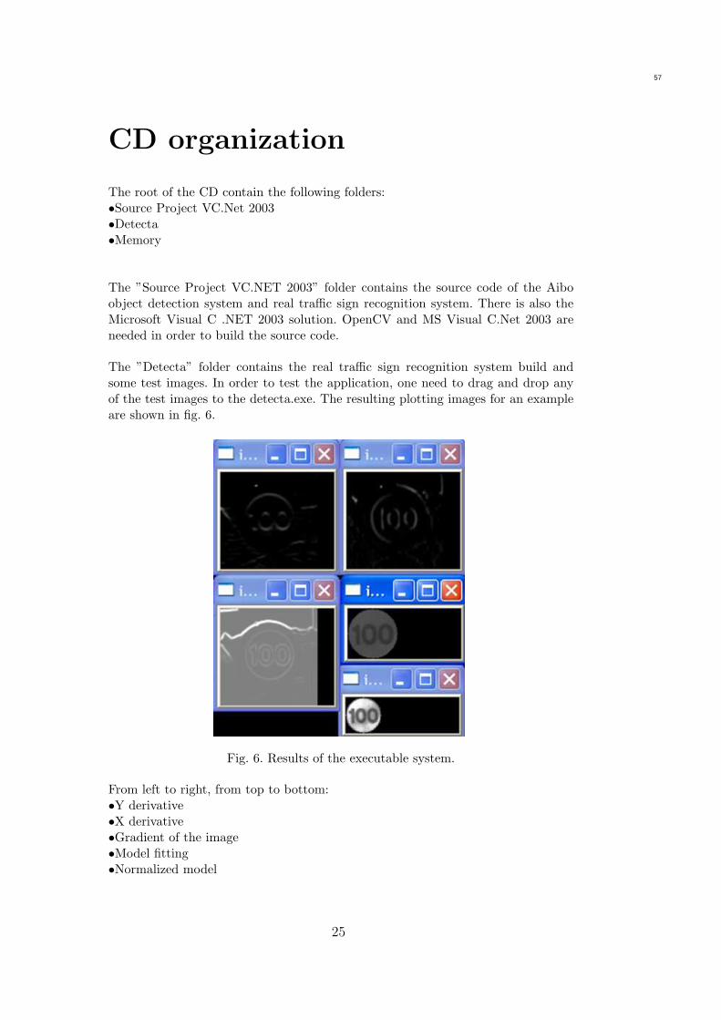
CD organization

The root of the CD contain the following folders:•Source Project VC.Net 2003•Detecta•Memory

The ”Source Project VC.NET 2003” folder contains the source code of the Aiboobject detection system and real traffic sign recognition system. There is also theMicrosoft Visual C .NET 2003 solution. OpenCV and MS Visual C.Net 2003 areneeded in order to build the source code.

The ”Detecta” folder contains the real traffic sign recognition system build andsome test images. In order to test the application, one need to drag and drop anyof the test images to the detecta.exe. The resulting plotting images for an exampleare shown in fig. 6.

Fig. 6. Results of the executable system.

From left to right, from top to bottom:•Y derivative•X derivative•Gradient of the image•Model fitting•Normalized model

25

57

The images remain plotted until any key is pressed. After to press any key, thesystem writes in the console the class membership of the input sample. If the K-NNclassifies the image as 100 (speed sign), the same image normalized by the FLDAclassification system is shown. Once a key is pressed, the console shows the signlabel.

The ”Memory” folder contains the article and documentation of the project.

26

58

2006