Embed Size (px)
Citation preview

Real-Time Face Detection on aConfigurable Hardware Platform
by
Rob McCready
A thesis submitted in conformity with the requirements
for the degree of Master of Applied Science in
the Graduate Department of Electrical and Computer Engineering,
University of Toronto
Copyright by Rob J. McCready 2000
ii
Real-Time Face Detection on a Configurable Hardware Platform
Rob McCready
Master of Applied Science, 2000
Department of Electrical and Computer Engineering
University of Toronto
Abstract
Automated object detection is desirable because locating important structures in an image is a fun-
damental operation in machine vision. The biggest obstacle to realizing this goal is the inherent
computational complexity of the problem. The focus of this research is to develop an object de-
tection system that operates on real-time video data in hardware. Using human faces as the target
object, we develop a detection method that is both accurate and efficient, and then implement it on
a large programmable hardware system. Using a programmable system reduced the time and cost
required to create a working hardware prototype. The implementation runs at 30 frames per second,
which is approximately 1000 times faster than the same algorithm running in software and approx-
imately 90 to 6000 times faster than the reported speed of other software algorithms.

iii
Acknowledgements
I am very grateful to my supervisor, Jonathan Rose, for his enthusiasm, patience, wisdom, hu-
mour, and unwavering confidence.
I am also indebted to Jonathan’s students both past and present for their advice and good com-
panionship, particularly Vaughn, Jordan, Yaska, and Sandy.
Dave Galloway and Marcus van Ierssel contributed much to this work in the form of TM-2a
support and maintenance.
I had the good fortune to work beside Mark Bourgeault, who had the poor fortune to encounter
many of the TM-2a bugs before I had to.
Ketan Padalia developed a neat serial arithmetic hardware generation tool for me to use. I
didn’t end up needing serial arithmetic, but the tool is neat nonetheless.
Prof. Allan Jepson, Chakra Chennubhotla, and Prof. James MacLean made time for some very
interesting and very useful conversations during the course of project.
My cubicle in LP392 would have been a very boring place to work without the always stimu-
lating presence of my colleages who also reside there (in 392, not my in cubicle).
I am grateful beyond measure for my family and friends, in particular for my partner Carly,
whose belief in my abilities is surpassed only by her love, for Mom, who is also sure I know what
I’m doing even though she remembers “FPGA” using the first initials of our relatives, and for my
sister Tara, who blazed the academic trail.

iv
Table Of Contents
Chapter 1: Introduction ........................................................................................................1
Chapter 2: Background ........................................................................................................32.1 Overview of Face Detection.............................................................................................................. 3
2.1.1 Problem Definition .................................................................................................................. 32.1.2 Face Detection as Object Detection ........................................................................................ 32.1.3 General Approach to Face Detection ...................................................................................... 5
2.2 Image Processing............................................................................................................................... 62.2.1 Image Filtering ........................................................................................................................ 72.2.2 G2/H2 Properties..................................................................................................................... 8
2.3 Pattern Classification......................................................................................................................... 92.3.1 Machine Learning.................................................................................................................... 92.3.2 Previous Pattern Classification Methods............................................................................... 132.3.3 Competitive Feature Analysis (CFA) .................................................................................... 18
2.4 Programmable Hardware................................................................................................................. 262.4.1 Field Programmable Gate Arrays (FPGAs) .......................................................................... 272.4.2 Reconfigurable Systems ........................................................................................................ 272.4.3 The TM-2a Reconfigurable System ...................................................................................... 28
2.5 Object Detection Using Reconfigurable Systems ........................................................................... 282.5.1 ATR Problem Description ..................................................................................................... 282.5.2 ATR Approaches ................................................................................................................... 292.5.3 Discussion ............................................................................................................................. 30
Chapter 3: Object Detection Framework ...........................................................................313.1 Goals and Assumptions ................................................................................................................... 32
3.2 Image Processing............................................................................................................................. 323.2.1 G2/H2 Filtering ..................................................................................................................... 323.2.2 QMP Conversion................................................................................................................... 33
3.3 CFA Classifier ................................................................................................................................. 353.3.1 Training Strategies................................................................................................................. 353.3.2 Hierarchy ............................................................................................................................... 383.3.3 Testing ................................................................................................................................... 39
3.4 Peak Detection................................................................................................................................. 41
3.5 Summary and Discussion ................................................................................................................ 41
Chapter 4: Hardware-Ready Face Detection .....................................................................444.1 Review of Framework ..................................................................................................................... 44
4.2 Filtering and QMP Conversion Parameters..................................................................................... 45
4.3 Object Detection Training and Testing............................................................................................ 454.3.1 Number and Scope of Features ............................................................................................. 464.3.2 Face and Non-Face Sets ........................................................................................................ 474.3.3 Feature Initialization.............................................................................................................. 474.3.4 Fixation and Repetition ......................................................................................................... 474.3.5 Bootstrapping ........................................................................................................................ 48
4.4 Detection Accuracy Results ............................................................................................................ 49

v
4.5 Discussion........................................................................................................................................ 49
Chapter 5: Hardware Implementation................................................................................515.1 Goals................................................................................................................................................ 51
5.2 Overview ......................................................................................................................................... 515.2.1 Flow Control.......................................................................................................................... 52
5.3 Video Input ...................................................................................................................................... 52
5.4 Scaling ............................................................................................................................................. 53
5.5 G2/H2 Filtering ............................................................................................................................... 545.5.1 Design Tools.......................................................................................................................... 555.5.2 X Filter Stage......................................................................................................................... 565.5.3 Y Filter Stage......................................................................................................................... 565.5.4 Comparison to Non-Separable Filters ................................................................................... 57
5.6 QMP Conversion ............................................................................................................................. 585.6.1 Efficiency of QMP ................................................................................................................ 58
5.7 Face Detection ................................................................................................................................. 595.7.1 FDU Structure ....................................................................................................................... 595.7.2 Design Tools.......................................................................................................................... 615.7.3 An Alternate Design.............................................................................................................. 61
5.8 Peak detection.................................................................................................................................. 62
5.9 Display............................................................................................................................................. 62
5.10Implementation Results ................................................................................................................... 625.10.1Functionality.......................................................................................................................... 625.10.2Speed ..................................................................................................................................... 635.10.3Accuracy................................................................................................................................ 64
Chapter 6: Conclusions and Future Work..........................................................................656.1 Conclusions and Contributions........................................................................................................ 65
6.2 Future Work..................................................................................................................................... 67
References .........................................................................................................................68
Appendix............................................................................................................................76

vi
List Of Figures
Figure 1: Object Pose Variation ...........................................................................................5
Figure 2: Face Detection Stages ..........................................................................................6
Figure 3: Frequency Response of a Vertical Bandpass Filter ..............................................7
Figure 4: G2/H2 Filters at 0 and 90 Degrees .......................................................................8
Figure 5: Structure of an Island-Style FPGA.....................................................................27
Figure 6: Detail of Logic Cluster Contents........................................................................27
Figure 7: Object Detection Processing Sequence ..............................................................31
Figure 8: G2/H2 Phase and Magnitude Calculation ..........................................................34
Figure 9: Phase Reflection .................................................................................................35
Figure 10: Pseudocode for Iterative Feature Addition/Removal .......................................37
Figure 11: Sample Input Arrays.........................................................................................39
Figure 12: Features Learned and Learning Progression During First-Level Training ......39
Figure 13: Second Level Feature Predictions for First-Level Feature Positions ...............40
Figure 14: Face Probability Surfaces.................................................................................41
Figure 15: Object Detection Processing Sequence ............................................................44
Figure 16: Probability of H2 Response (normalized to [0,255]) .......................................50
Figure 17: Block Diagram of Face Detection System .......................................................52
Figure 18: Structure of Scaling Unit..................................................................................53
Figure 19: Scaling Unit Processing Stages ........................................................................54
Figure 20: Example Structure of a 5-element X Filter ......................................................56
Figure 21: Example of 7x7 Shifter Array Operation .........................................................57
Figure 22: Face Detection Unit Principle and Structure....................................................59
Figure 23: Face Detection Hardware Output .....................................................................63

1
Chapter 1
Introduction
Humans use vision as their primary means for gathering information about, and navigating
through, their surroundings. Providing this ability to automated systems would be a large step to-
ward having them operate effectively in our world. There are, however, two major obstacles to au-
tomated vision: incomplete human knowledge of how to reliably derive high-level information
from a 2-D image; and the computational complexity of image processing and analysis methods.
The latter is of primary concern in the research and development of real-time systems.
Only recently has the growth in affordable computing power and research into faster tech-
niques allowed some complex vision tasks to move into industrial and consumer applications.
Since many of the most compute-intensive image processing operations are also highly parallel
they could be accelerated by orders of magnitude using a customized hardware implementation.
This is widely recognized in real-time vision research but rarely attempted since the resources re-
quired to design custom hardware are usually not available. Instead researchers direct their efforts
toward devising vision algorithms that are efficient when implemented using standard processors.
They thus avoid due to computational complexity approaches which are not feasible in software
but might work well in hardware.
Another option not widely known in the vision community to employ programmable hardware
as the implementation vehicle. Programmable hardware has already been shown to be a good so-
lution for many signal processing tasks that are similar to machine vision [25][26][27][28], and us-
ing a programmable system reduces the time, cost, and expertise required to create a working
hardware prototype. It reduces cost by avoiding the enormous expense of chip and board fabrica-
tion and by spreading the cost of the system over all of the vision and non-vision applications for
which it might be used. It reduces time and expertise requirements by permitting less rigorous de-
sign and testing. When using programmable hardware, the cost of fixing a bug after design is the

Chapter 1: Introduction 2
minimal penalty of recompiling rather than the enormous expense of refabricating. The cost of a
design change is similarly reduced, thus allowing much more experimentation using differing
hardware implementations.
The goal of this research is to explore the feasibility of programmable hardware as a platform
for complex real-time machine vision. We will do this by implementing a complex vision task on
the Transmogrifier-2a (TM-2a), a large configurable hardware system [18][19]. The vision prob-
lem we will focus on is object detection: the task of locating an object in an image despite consid-
erable variation in lighting, background and object appearance. Object detection is one of the best-
known and most useful machine vision applications, and is also difficult and computationally com-
plex. The specific case we will consider is face detection, motivated because face analysis is a very
active area of vision research. Face analysis can be used in security applications, telecommunica-
tions, human-computer interfaces, entertainment, and database retrieval. In order to analyze a face
in detail, however, the face must first be located. Many face analysis algorithms are developed with
the assumption of controlled environments in which face detection is trivial. Such assumptions be-
come invalid as the applications move into uncontrolled environments, so accurate face detection
is necessary. Since detection is only a first step before recognition and other tasks, it needs to be
done quickly.
The first stage of this research was to develop an object detection strategy that would be accu-
rate, efficient in hardware, and applicable to faces. The literature proposes a considerable variety
of approaches, but the best of these are either inherently serial or require too much hardware to im-
plement. We have developed an object detection framework aimed at a hardware implementation
and based on a new machine learning method. The second stage was the adaptation of the frame-
work for the specific problem of face detection. The third and final stage was to implement the
method on a programmable hardware system. The final implementation runs at 30 frames per sec-
ond and detects faces over three octaves of scale variation. This is approximately 1000 times faster
than the same algorithm running in software on a 500MHz UltraSparc and approximately 90 to
6000 times faster than the reported speed of other software algorithms.
This dissertation begins by presenting background in Chapter 2. Chapter 3 presents the object
detection framework, and Chapter 4 discusses its use for face detection. Chapter 5 describes the
implementation of the face detection algorithm in programmable hardware. Finally, Chapter 6 pre-
sents conclusions and future work.

3
Chapter 2
Background
This thesis has two goals: to develop a face detection method that is both accurate and efficient
in programmable hardware; and to implement this algorithm on a large programmable system. In
this chapter, Section 2.1 first reviews the face detection problem and presents a general face detec-
tion approach. Sections 2.2 and 2.3 then consider in detail two stages of this general approach: im-
age processing and pattern classification, respectively. Section 2.4 looks at programmable logic
and programmable hardware systems, and Section 2.5 reviews how these have been used to per-
form tasks similar to the one at hand.
2.1 Overview of Face Detection
2.1.1 Problem DefinitionFor this thesis, face detection is defined as the problem of locating faces in an image in the pres-
ence of uncontrolled backgrounds and lighting, unrestricted range of facial expression, and typical
variations in hair style, facial hair, glasses, and other adornments. These variations must be handled
by any face detection method which hopes to operate in an uncontrolled environment. We do not
assume the presence of colour information, motion information, or other parts of the body, since
the human vision system proves that it is possible to detect faces without them, and they would
introduce additional potential failure modes for the system.
2.1.2 Face Detection as Object DetectionThe problem of face detection falls into the much larger category of object detection. Although
the terms “detection” and “recognition” are often used interchangeably in the literature, we define
them as follows: given one or more object classes, “detection” is the task of distinguishing mem-
bers of one class from members of another, and “recognition” is the task of distinguishing between
members of the same class. The ambiguity between these two problems comes from the fact that

Chapter 2: Background 4
whether one is doing detection or recognition depends entirely on how one defines the object class-
es.
In the most typical detection problem there are only two classes: the class of target objects (fac-
es, for example) and the class of all other objects, or the background class. Any object detection
problem that fits this model is then uniquely defined by two factors: the variation in the target ob-
ject’s appearance; and the variation in the appearance of all of the non-target objects. If either of
these kinds of variation is not present, accurate detection becomes trivial. If the target objects ap-
pear against an unvarying background then detection consists of a simple subtraction operation,
even if the object itself varies wildly in appearance. If the target objects have a precise, unvarying
visual appearance then detection can be performed by a matched filter even in nearly arbitrary clut-
ter. In the most interesting detection problems there is significant variation in both the appearance
of the target objects and the appearance of the background, such that there exist instances of each
class that are indistinguishable from instances of the other.
Face detection is one of these problems. Faces can change drastically in visual appearance from
one individual to the next and even for a single individual over the space of expression, facial hair,
and adornments such as glasses. Due to their 3-dimensional structure, the appearance of faces also
depends greatly on lighting conditions. As for backgrounds, they are essentially arbitrary; when
one considers the space of likely surrounding objects, both natural and man-made, we are able to
exclude from possibility only the most unnatural kinds of artificially generated noise.
One source of target appearance variation that is common to all visual detection problems is
object pose. The three types of pose variation are illustrated in Figure 1. Objects can vary in size
depending on their distance from the camera, and they can be rotated through three degrees of free-
dom. Changes in size and rotation in the camera’s image plane pose only a computational problem
as in any case the image could be scaled or rotated to correct for them. Rotation in depth poses a
much more serious problem as the resulting appearance depends on the three-dimensional structure
of the object. One useful way to categorize detection methods is by the extent to which they can
tolerate variation in the different components of object pose, and we will consider this when we
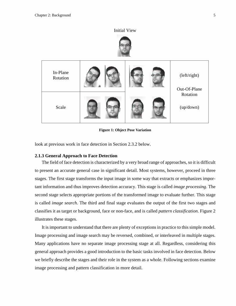
Chapter 2: Background 5
look at previous work in face detection in Section 2.3.2 below.
2.1.3 General Approach to Face DetectionThe field of face detection is characterized by a very broad range of approaches, so it is difficult
to present an accurate general case in significant detail. Most systems, however, proceed in three
stages. The first stage transforms the input image in some way that extracts or emphasizes impor-
tant information and thus improves detection accuracy. This stage is called image processing. The
second stage selects appropriate portions of the transformed image to evaluate further. This stage
is called image search. The third and final stage evaluates the output of the first two stages and
classifies it as target or background, face or non-face, and is called pattern classification. Figure 2
illustrates these stages.
It is important to understand that there are plenty of exceptions in practice to this simple model.
Image processing and image search may be reversed, combined, or interleaved in multiple stages.
Many applications have no separate image processing stage at all. Regardless, considering this
general approach provides a good introduction to the basic tasks involved in face detection. Below
we briefly describe the stages and their role in the system as a whole. Following sections examine
image processing and pattern classification in more detail.
Initial View
In-PlaneRotation
Scale
Out-Of-PlaneRotation
(up/down)
Figure 1: Object Pose Variation
(left/right)

Chapter 2: Background 6
Any given face detection system could use a considerable variety of image processing tasks, as
the particular ones chosen will depend on the requirements of the pattern classification stage. The
processing stage must extract information that the classification stage needs and suppress variation
that the classification stage cannot handle. Two common tasks are lighting correction and filtering.
Lighting correction reduces the effects of variable lighting intensity and direction, and filtering ex-
tracts information at particular spatial frequencies and orientations. Section 2.2 below discusses
image processing.
The image search method chosen also depends on the capabilities of the pattern classification
stage. One very simple and common method is to systematically select every possible sub-image
from the input, potentially including scaled and/or rotated sub-images in order to compensate for
face size and in-plane rotation. This is often used for fixed-size face “templates”. The approach is
computationally expensive, however, and so recent work has focussed on developing ways to re-
duce the search space. In some cases, additional information such as colour or motion is used to
find portions of the image which are likely to contain a face. In other cases, the classification step
is designed to either be inherently invariant with respect to scale or rotation, or designed to provide
a method of directed image search.
Pattern classification is the most critical and complex of the three stages. The accuracy of the
face detection system relies primarily on the performance of this stage, and faces, as we discussed
above, are particularly difficult to classify because of the amount of possible variation in both face
appearance and background appearance. Section 2.3 below discusses pattern classification.
2.2 Image ProcessingThe first stage in our general face detection model is image processing. This stage must trans-
form the incoming data such that it is suitable for use by pattern classification. One common image
processing tool, image filtering, is an important stage in many vision systems because it emphasiz-
es certain types of information in an image and suppresses others. In this thesis we use a specific
pair of filters called G2 and H2 [16]. Below we give an overview of the image filtering process and
Figure 2: Face Detection Stages
ImageProcessing
PatternClassification
ImageSearch
Chapter 2: Background 7
then describe the properties of these filters in detail.
2.2.1 Image FilteringThere are many types of filters and many kinds of image data on which they operate, but we
are only going to consider one case: linear FIR filters operating on greyscale images. An FIR image
filter consists of a two-dimensional array of coefficients sampled from the filter’s continuous im-
pulse response. This is often called the filter kernel. The filter output for an image is generated by
performing a 2-D convolution operation between the image and this kernel. One useful way to vi-
sualize the filtering process is to imagine the kernel sliding across the image surface such that it is
centered, in turn, over each pixel location in the image. At each location each kernel coefficient is
multiplied with the greyscale value directly underneath it. The filter result for that location is the
sum of these products. Those familiar with 1-D FIR filtering or convolution will recognize this as
a simple extension to two dimensions.
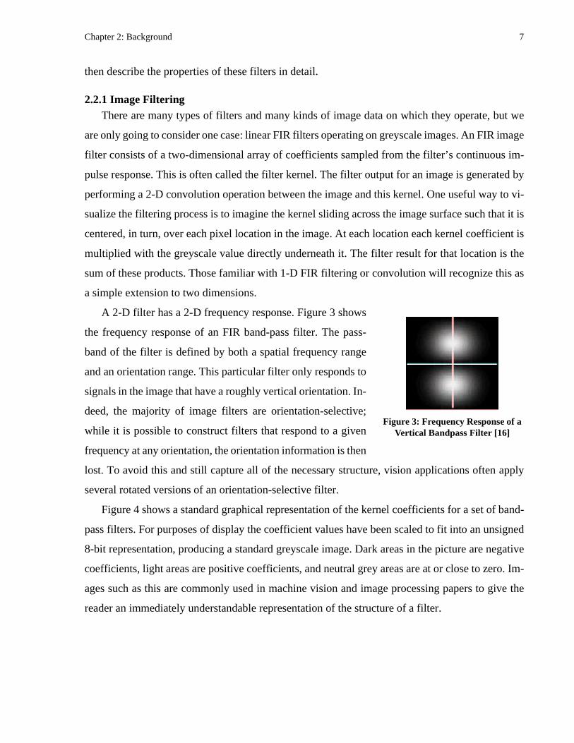
A 2-D filter has a 2-D frequency response. Figure 3 shows
the frequency response of an FIR band-pass filter. The pass-
band of the filter is defined by both a spatial frequency range
and an orientation range. This particular filter only responds to
signals in the image that have a roughly vertical orientation. In-
deed, the majority of image filters are orientation-selective;
while it is possible to construct filters that respond to a given
frequency at any orientation, the orientation information is then
lost. To avoid this and still capture all of the necessary structure, vision applications often apply
several rotated versions of an orientation-selective filter.
Figure 4 shows a standard graphical representation of the kernel coefficients for a set of band-
pass filters. For purposes of display the coefficient values have been scaled to fit into an unsigned
8-bit representation, producing a standard greyscale image. Dark areas in the picture are negative
coefficients, light areas are positive coefficients, and neutral grey areas are at or close to zero. Im-
ages such as this are commonly used in machine vision and image processing papers to give the
reader an immediately understandable representation of the structure of a filter.
Figure 3: Frequency Response of a Vertical Bandpass Filter [16]

Chapter 2: Background 8
2.2.2 G2/H2 PropertiesG2 and H2 are members of a class of filters useful for a
range of machine vision tasks [16][17]. Figure 4 shows the ker-
nels of the 0 and 90 degree orientations of both G2 and H2. G2
is the second derivative of a Gaussian, and H2 is the Hilbert
transform of G2. For the purposes of this work, they have three
important features: they are band-pass filters that form a
quadrature pair and are thus useful tools for multi-scale texture
analysis; they are X-Y separable, which makes them efficient
to implement; and they are orientation-steerable, which allows us to generate a version of the filters
at any orientation using a fixed set of basis filters.
An X-Y separable filter has an impulse response that may be expressed as a product of two
functions: one which depends only on X, and one which depends only on Y. Consider a the sepa-
rable filter with kernel defined as:
(EQ 1)
If we convolve with the image to produce the filter output , we can
separate the convolution into separate X and Y stages:
(EQ 2)
where is the size of the filter kernel. The image is first convolved with a row vector of X
coefficients, and then these X results are convolved with a column vector of Y coefficients. This
reduces the filtering process from an operation to an operation.
The other important property of G2/H2 is orientation-steerability. An orientation-steerable fil-
ter is one that can be generated at any orientation using linear combinations of a finite set of basis
filters. For G2, three basis filters are required; for H2, four are required. This property contributes
further to the pair’s efficiency, because it restricts the number of unique filter kernels convolved
with the image to seven, regardless of the number of distinct filter orientations the application
needs. If we only needed one or two orientations, however, we would probably not bother to use
G2
H2
0° 90°
Figure 4: G2/H2 Filters at 0 and 90 Degrees
K x[ ] y[ ]
K x[ ] y[ ] F x[ ] G y[ ]•=
K x[ ] y[ ] I x[ ] y[ ] O x[ ] y[ ]
O x[ ] y[ ] G v[ ] F u[ ] I x u+[ ] y v+[ ]•u N 2⁄( )–=
N 2⁄
∑
•v N 2⁄( )–=
N 2⁄
∑=
N
O N2( ) O 2N( )
Chapter 2: Background 9
this property as the cost of applying all of the basis filters would exceed the cost of directly apply-
ing the oriented filter versions.
2.3 Pattern ClassificationThe final stage in our general face detection system is pattern classification. Pattern classifica-
tion takes as input an image region enhanced by the processing stage and selected by the search
stage. As output it produces a decision as to whether the region represents a face or represents back-
ground. All face detection methods must use some form of pattern classification to distinguish fac-
es from background, and the accuracy of this classification is the most important contributor to the
overall accuracy of the system. When designing a face detection system, it is therefore critical to
design an accurate pattern classification method. In this section we first discuss one of the most
powerful techniques for constructing accurate classifiers: machine learning. We then review clas-
sification methods used in previous work and analyze their performance. Finally, we present the
machine learning method on which the classifier used in this work is based.
2.3.1 Machine LearningFace detection is a difficult task because of the variation present in both face and background
appearance. Given the complexity of the problem, it is difficult to hand-craft a solution that will
have satisfactory accuracy. Instead, one of the best ways to build a classifier is to collect a large set
of classification examples, create a parameterized classification function, and then have a computer
optimize the function parameters such that the output better agrees with the examples. This process
is called machine learning. Machine learning methods approximate the underlying statistical prop-
erties of an unknown system by observing the system’s behaviour. The unknown system is repre-
sented by a parameterized model, and it’s behaviour is captured in a set of samples called a training
set. An optimization algorithm modifies, or “trains”, the model parameters such that the error be-
tween the model’s predictions and the training set data is minimized.
In the absence of machine learning, application designers must rely on their own domain
knowledge to create an approximation of an unknown system. This process is highly susceptible
to the often incomplete and inaccurate nature of human memory and reasoning. If the system is
very complex, accurately hand-crafting an approximation may not be possible at all. In contrast, a
machine learning method has only those biases explicitly included in the model and optimization
procedure. Even for very complex systems machine learning provides a directed means to search

Chapter 2: Background 10
the space of model parameters and provide a result that fits the examples given and generalizes to
new ones.
Many machine vision applications use machine learning concepts. An image of a scene is a
very under-constrained description of that scene’s contents, and thus machine vision techniques
must be given a good deal of prior knowledge about the structures they are looking for in order to
extract any information at all from the data. Machine learning techniques allow this prior knowl-
edge to be captured from examples of the structures rather than explicitly stated. The most accurate
face detection techniques are those which make consistent use of machine learning, as we discuss
in Section 2.3.2 below.
In this section we first review the major styles of machine learning, which we divide into su-
pervised and unsupervised methods. We then describe general machine learning issues around
choice of model, model training, and model testing.
Styles of Learning
There are two major styles of machine learning: supervised and unsupervised. Both styles have
been used in the face detection systems we will discuss, and the learning method used in this work
combines elements of both. It is important to understand the different goals and characteristics of
each type to evaluate how choosing one or the other can affect the performance of a face detection
system.
Supervised learning refers to methods in which each training example has two sets of values:
a set of known inputs and a set of target outputs. The goal of training is to have the model produce
the correct outputs when presented with particular inputs. These methods are given the label “su-
pervised” by analogy to a human learning process in which the learner is monitored and corrected
at each step. This category includes the most widely known and used learning techniques, ranging
from polynomial fitting to artificial neural networks.
While supervised learning approximates input/output relationships, unsupervised learning ap-
proximates generative processes. Given a training set of patterns from a single target class, the goal
of unsupervised learning is to learn a model of the statistical structure of the patterns. Once trained,
such models are often used to calculate the probability that a new pattern belongs to the target class,
to encode and then reconstruct patterns, or to generate completely new example patterns that con-
form to the learned statistics. These methods are labeled “unsupervised” since no explicit target
output values are given, but it is important not to take this label at its semantic face value. In a very

Chapter 2: Background 11
real sense the data themselves are both the known input and the target output, as many unsuper-
vised learning methods measure their performance by coding an example, reconstructing it, and
then comparing the reconstruction with the original. In order for these methods to work, human
intervention is still required to ensure that the training set contains only positive examples of the
target class.
Unsupervised learning methods are generally less well-known than supervised methods, but
they have proven to be very powerful and useful tools. The basic idea behind unsupervised learning
can be summarized as “representation equals analysis”: if we try to learn ways to accurately and
efficiently represent the target patterns, we are likely to end up discovering interesting structure
about those patterns. This emphasis on representation and reconstruction makes unsupervised
learning excellent for problems such as efficient domain-specific video or sound coding tech-
niques. Unfortunately, it is not so well suited to detection problems. When performing detection,
we are interested in what differentiates our target pattern from other non-target patterns that are
likely to occur. Unsupervised learning only analyses the target pattern with the goal of representing
it, and the details that are useful for accurate representation are not always or even usually the de-
tails that are useful for detection.
Models, Training, and Testing
Even with the wide variety of approaches to machine learning, there are three steps that most
application designers perform: choose a model architecture; train the model; and test the perfor-
mance of the trained system. Although the details of these steps vary considerably from method to
method, there are general guidelines and theory on how to perform them so as to encourage good
performance and ensure accurate measurement of that performance. In this section we discuss typ-
ical ways of approaching these tasks.
Many machine learning methods require the designer to choose a specific model architecture.
It is important to choose an architecture with an appropriate level of complexity and an appropriate
internal structure. The complexity of a model is determined largely by the number of free param-
eters, and the greater the number of model parameters, the greater representational power the mod-
el has. If a model is too simple it will not be able to capture the underlying structure of the target
system and will perform badly. For example, a linear model could never fit quadratic data accu-
rately. This is called bias error. If the model is too complex it will be under-constrained by the
training set and will over-fit it, causing poor performance on new data. For example a, 9th-order

Chapter 2: Background 12
polynomial fits any set of 10 training points precisely, including any noise in the data. This is called
variance error. Closely related to the issue of choosing model complexity is that of choosing model
structure. With many learning techniques the designer has the opportunity to impose certain struc-
tural constraints on the model. Doing so reduces the number of model parameters by removing
those which would have allowed the model to move away from the imposed structure. If the struc-
ture is guided by knowledge about the target system, however, we can reduce the number of model
parameters without reducing the effectiveness of the model; we reduce the variance error without
adding bias error. Choosing model structure is something of an art because of this. Although hu-
man domain knowledge is problematic when it comes to manually defining the gritty details of an
approximation, it is typically the best way to craft a model structure to learn those details. Even so
it remains a good idea to mitigate the designer’s biases by training a set of models with different
structures and complexity, and either keeping the best one or combining their results in some fash-
ion.
Once a model is chosen the next step is to train it, and the most important component of training
is the training set. When it comes to training sets, one can rarely have enough data. Having a large
number of samples is one of the best ways to ensure good results. Sheer number of examples, how-
ever, is not the only consideration. Ensuring that the training set covers a broad variety of operating
circumstances is also vital. The learning algorithm will find whatever statistical relationships exist
in the data, even the ones that occur by accident, and it will not find those relationships which do
not exist in the data. There are many cases of machine learning systems that were trained on data
that had strong spurious correlations and thus performed in very strange ways once deployed. As
an example, consider what might happen if a face detection algorithm were trained with a set of
face images taken with the subjects standing against a brick wall. The trained model might include
more information about the structure of the wall than about the structure of the faces. In operation
it might do a great job of detecting brick walls, but be utterly unable to find a single face.
In practice, it is almost never possible to achieve either the number or variety of training set
examples required to avoid over-fitting altogether. To address this problem, machine vision re-
searchers have developed the concept of regularization. Regularization places soft a priori con-
straints on parameter values during training that encourage the model as a whole to prefer simpler
solutions over more complex ones. These constraints are set to be weak enough that the major re-
lationships in the data are learned and strong enough that the occasional spurious correlations are

Chapter 2: Background 13
smoothed away.
Finally, we need to be able to estimate the performance of the trained system on new data. For
this purpose we use a test set, which is a set of data not included in training but only used to deter-
mine the accuracy of the system. Typically the designer will randomly select 10% of the available
examples and reserve them for the test set, leaving the remaining 90% for training. Training is re-
peated several times with different randomly selected test and training sets and the results are av-
eraged. This ensures that the measured accuracy is not influenced by the unlucky choice of a test
set that is not representative of the data as a whole.
2.3.2 Previous Pattern Classification MethodsIn this section we review and discuss a number of recent approaches to pattern classification in
face detection. At the beginning of this chapter we gave a definition of the specific face detection
problem considered in this work. Even with this limiting definition, however, there are a large
number of differing approaches in prior work to examine and compare. To reduce this number, we
will only consider appearance-based approaches: those that model a face as one or more two-di-
mensional patterns and do not have an explicit three-dimensional description of head or face struc-
ture. Viewed as two-dimensional patterns of intensity variation, faces are objects with distinct sub-
patterns that occur over scopes ranging from highly local to nearly global. Over the space of iden-
tity, expression, lighting, and pose these patterns can deform and move independently with respect
to one another.
The key to accurate face detection is to identify those patterns which are stable over the space
of face appearance and are useful for distinguishing faces from background, and then to unify these
patterns in a flexible manner into a whole face detector. As we review previous face detection clas-
sifiers, we will be considering in particular how each is biased towards particular types and scopes
of patterns, how each determines which patterns to use, and how these patterns are connected. At
the end of the section we will summarize and synthesize the prior work and use this analysis as the
basis for developing a robust face detection method.
The simplest appearance-based face detection method is perhaps the matched filter or correla-
tion template. The template consists of a single, properly normalized (for statistical purposes) im-
age of a face. The template is created by averaging a training set of face images, which is a very
simple type of unsupervised learning. This kind of method does not typically perform well for the
simple reason that a single fixed template is too inflexible to capture enough appearance variation.

Chapter 2: Background 14
A single template represents all face patterns from local to global with a single mean case, and rep-
resents them together in a rigid spatial arrangement. Even if the training images are normalized for
position and scale with respect to some facial landmarks, independent movement or deformation
of patterns associated with other landmarks will result in a blurring effect after averaging. Patterns
with global scope tend to be affected little by this, while very local patterns may be entirely ob-
scured, so such methods favour global patterns.
There have been a number of methods which improve on the basic correlation template by di-
viding the face into separate local regions and using more complex learning methods to capture
greater variation. Mogghadam and Pentland [6] use four regions corresponding to four facial land-
marks: left eye, right eye, nose, and mouth. They use an unsupervised learning technique called
Principal Components Analysis (PCA) to model the variation in these features. PCA generates a
mapping from the high-dimensional input pixel space to a lower-dimensional feature-specific
space. Once PCA has determined this mapping, two measures are used to decide whether a partic-
ular sub-image matches a feature: a measure of how much of the information in the image is lost
by the mapping; and a measure of how likely it is that the mapped point corresponds to a valid fea-
ture. These probabilistic measures are determined by another unsupervised learning stage. A third
unsupervised learning stage models the spatial relationships between the four features. On a very
simple test set with little variation, this method detects 90% of the faces. One of the major draw-
backs of this approach is that no attempt is made to model and account for close non-face patterns:
PCA finds a mapping which is optimal for face representation but which may not be useful for clas-
sification. Lew [4] addresses this problem by using a very similar method with two major differ-
ences. First, a supervised learning stage analyses face and non-face images and determines which
pixels are the most important for distinguishing faces from background. Second, the authors use a
supervised learning method which is similar to PCA, but which finds a mapping directed towards
classification.
The methods discussed above have solved the correlation template’s problem of representing
local and global patterns together in a single template by splitting that template into a set of smaller
ones that can vary independently. While doing so improves the flexibility of the model, it also ig-
nores a considerable amount of information. These methods place absolute limits on pattern scope;
patterns which would extend beyond the size of any single smaller template can no longer even be
represented. They also require a choice of which sub-patterns to pay attention to; while a single

Chapter 2: Background 15
whole-face template can at least attempt to represent all face patterns, a set of local templates can-
not represent any pattern that falls outside of the chosen sub-regions. This choice of pattern is made
manually, and so is subject to all of the inaccuracies of human reasoning.
Leung et. al. [14] illustrates an extreme case of sacrificing information for flexibility. They use
a face model consisting of local pattern detectors connected via a complex shape model. The pat-
terns and shape model are invariant with respect to in-plane rotation and scale, and are also very
tolerant with respect to out-of-plane rotation. The resulting model can predict the positions of miss-
ing features during search and evaluate the quality of a face candidate by calculating its probability
under the model parameters. The authors chose a multi-orientation, multi-scale set of derivative-
of-Gaussian filters to describe 12 facial landmarks. The responses of a given landmark to these fil-
ters are assembled into a vector that serves as a landmark template. At run time the same filters are
convolved with the input image producing a similar vector at each location. These vectors are com-
pared with the feature vectors to determine where the local patterns are present. The individual
landmark detectors are, however, fairly unreliable. Each generates a large number of false posi-
tives. The authors use their shape model to look for groupings of multiple local features that con-
form to the expected arrangement
While this method inherently deals well with variation due to face pose, it does not deal well
with variation due to other factors such as identity and expression; the authors report a detection
accuracy of only 70%. The likely reason is that the small number of very local features do not take
enough information into account, so that faces that happen to vary considerably in those particular
areas cannot be detected. While the local pattern vectors and the spatial relationship model are
trained using unsupervised learning, the choice of facial landmarks is manual and thus arbitrary.
Part of the degradation in performance could be due to using landmarks that are not truly stable
indications of the presence of a face. This stability can only be judged reliably by a rigorous statis-
tical learning method.
The most successful techniques find ways to balance local and global scopes and balance in-
formation versus flexibility. The key to doing this well is to use machine learning to decide what
information is truly important. To this end Rowley et al. [10][11] propose a neural network face
detection system. The system has a 20x20 pixel receptive field which is applied at every location
in the input image. The network is structured to allow for both a small set of large patterns and larg-
er set of local patterns. The candidate sub-image is passed into this detector network, which is

Chapter 2: Background 16
trained to produce a “1” on its output if the area contains a face, and a “-1” otherwise. One problem
associated with training a face detection network using supervised learning is that it is difficult to
manually choose challenging non-face examples, as one never knows beforehand what cases the
network will classify badly. To overcome this problem the authors use a “bootstrap” training meth-
od; areas which are incorrectly identified as faces are included more often in subsequent training.
The final system arbitrates between a redundant pair of independently trained networks to produce
greater accuracy. Several different network architectures and arbitration schemes were used pro-
ducing differing levels of accuracy, but in general the detection rate was 85% to 90% with few false
positives. The good performance of the system and the widespread acceptance and understanding
of neural networks have made this method popular. McKenna et. al. [9] use the detector net from
[10] as a verification stage in their motion-based face detection system. Han et. al. [5] also use the
detector as a verification stage. The major limitation of this approach is the hand-crafted structure
of the network; while it is useful and intuitive, it also places hard limits on the sort and arrangement
of information the network can use.
Schniederman [12] uses a very different modelling technique and produces better results still.
The face is modelled by a discrete set of patterns combined at different positions and over three
different scales. The likelihood of a particular pattern type occurring at any given position and scale
is calculated for both faces and non-faces, and this information is used during run-time to classify
candidate image regions. The multi-scale nature of the model allows a considerable range of pat-
tern scopes to be accounted for, and the explicit comparison with non-face distributions causes pat-
terns with little discriminatory power to be ignored. Using the same test set as Rowley et al., this
system produces a 10% better detection rate given the same number of false positives.
Discussion
From our review of pertinent current methods, we can see some general approaches that work
well. A robust face detection method is able to accurately account for patterns with varying scope,
from local to global. This typically involves breaking up the face into a set of independent patterns
and allowing these patterns to move in relation to one another. As much as is possible, the scope,
location, and arrangement of these patterns is learned rather than chosen manually, and the learning
process focusses on discriminating between faces and non-faces rather than on attempting to accu-
rately represent face images alone. Once the useful patterns have been identified they have to be
flexibly integrated into a whole face detector, either implicitly as in multi-layer neural networks or

Chapter 2: Background 17
explicitly via statistical models of pattern position.
The methods we reviewed each satisfied these goals to different degrees and in different ways.
One thing that is common to nearly all, however, is that the designers needed to assemble a hodge-
podge of techniques: shape statistics, Gaussian clustering, neural networks, supervised learning,
unsupervised learning, and large contributions of manual construction. There are two examples in
which this mixing of techniques is most obvious. The first is the selection of pattern locations and
scopes. In all of the methods we reviewed there is a significant amount of designer choice required
in determining the possible location and scope of patterns used, if not required in determining the
patterns themselves. Even in Rowley et al. [10] the network architecture allowed only three differ-
ent pattern scopes and a distinct set of positions, and this is also true of Schniederman [12]. The
second example is the separation between the detection methods used to find individual patterns
and the unification methods used to find a characteristic arrangement of the patterns. In all but
Rowley et al. [10] the method used to detect pattern arrangements had no relationship to the meth-
od used to detect the patterns themselves.
We have discussed at several points why designers should avoid inserting arbitrary decisions
into their systems, but have not touched on any benefits of using a single learning method rather
than a combination of methods. What we would ideally like is for both the task of learning a char-
acteristic arrangement of patterns and the task of learning the patterns themselves to be expressed
in a single theoretical framework. There are two major benefits of this: elegance and extensibility.
Elegance is a badly defined term, but we would consider an elegant solution to be one which ac-
counts for the required complexity within a rigorous framework and without significant special
case requirements. This is of greatest importance during design as it avoids ad-hoc solutions to
parts of the problem that are otherwise not handled. Extensibility comes as a result of considering
the unification stage to be an additional detection stage in which we look for patterns in the outputs
of the initial pattern detectors. We can learn patterns in these outputs exactly the same way as we
learn patterns in the input by simply repeating an identical second stage of analysis on top of the
first. In the same way as we looked for different scales and types of patterns in the input, we now
look for them again in the pattern detection results. Once we are able to perform this analysis
“stacking”, we can repeat it as many times as required by the structure of the data. The standard
ANN is a good example of a learning method that displays these properties; neurons in the first
layer are sensitive to certain patterns in the input, neurons in the second layer are sensitive to cer-
Chapter 2: Background 18
tain patterns in the first layer, and so on. Each neuron, regardless of where it is located, is trained
and activated in precisely the same manner as any other neuron. This has proven to be a very ele-
gant, extensible, and useful method indeed. The major difficulty with ANNs from our perspective
is that the designer must manually craft a network architecture, thus limiting the types of patterns
the net can use.
Any single method that is going to satisfy these requirements will have to be able to perform
two tasks automatically: decompose the input into an appropriate set of stable, characteristic pat-
terns; and build an appropriate hierarchy of pattern detectors by applying this decomposition at
more than one level of analysis. In the next section we discuss the CFA algorithm we use in our
own face detection application and which was developed to perform this sort of analysis.
2.3.3 Competitive Feature Analysis (CFA)In the previous section we reviewed some past and current face detection methods in order to
evaluate what strategies were the most successful and why. We found that the best methods used
machine learning techniques to discover the important patterns in the input and to model how these
patterns are arranged. All of the existing approaches, however, need significant human intervention
to limit the scope and position of potential patterns, and all save one use completely different meth-
ods to learn the patterns and then learn their spatial arrangement. In the conclusion, we noted that
what was needed was a method that could perform both automatic decomposition, to find impor-
tant patterns, and automatic hierarchy building, to unify them.
This section describes the Competitive Feature Analysis (CFA) learning method. CFA was de-
veloped at the beginning of this work with visual object detection specifically in mind, although it
is not considered part of this thesis and will be developed in future research. Presented with a train-
ing set of object images, CFA is designed to decompose the object into characteristic sub-patterns
through the use of competing pattern detectors called features. Each feature is responsible for a par-
ticular pattern present in the object’s appearance, and the features compete with each other to be
responsible for larger portions of the object. Features have nonlinear outputs which may be used
as inputs to higher-level features in a hierarchy, providing an elegant method of pattern unification.
The competitive learning algorithm strongly couples representation with detection and provides an
elegant way to integrate non-target examples. This approach ensures that the patterns learned are
both stable and characteristic of the target class.
We first discuss the particular type of inputs required by features and examine how a feature
Chapter 2: Background 19
internally represents the pattern for which it is responsible. Next we show how this representation
is used to produce a detection probability given input, and also how it is used to reconstruct input
given a detection probability. This is followed by a discussion of the competitive learning algo-
rithm. We briefly look at feature hierarchies, and finally summarize the properties of the CFA
method. In order to avoid unnecessary detail in this section only simplified versions of the most
important CFA formulas are shown. Appendix A contains the full formulation for those interested.
Feature Inputs
One unusual aspect of CFA features is the type of inputs they use. CFA has a probabilistic for-
mulation, and as part of this formulation it requires that feature inputs are in the form of probabil-
ities. This is different from most other learning methods, which can typically operate on any real-
valued input. It also seems problematic for visual detection, as greyscale images are expressed as
real-valued pixels, not probabilities.
To evaluate the implications of this input requirement, it is instructive to review some basic
probability theory. Any probability specifies the likelihood of a random event, and this random
event is defined as the occurence of a random variable meeting certain criteria. CFA requires that
the variables associated with feature inputs are discrete, meaning that each can only take on a set
of mutually exclusive states. These states constitute the sample space of the random variable. A
good example of a discrete random variable is the typical speed switch on a fan, which might have
the settings “off”, “low”, and “high”. The switch cannot take on values between these states, and
it must always be in one state or another. The current state of the fan switch can be represented by
a set of probabilities. For example, the set {0.1, 0.6, 0.3} indicates that there is a 10% chance that
the switch is “off”, a 60% chance that it is on “low”, and a 30% chance that is on “high”. Since the
switch is always in one of these states, the probabilities in the set must sum to one
The state of an input to a CFA feature is similary represented by a probability set. The practical
result of this requirement is that the designer of a CFA-based detection application must determine
beforehand a discrete representation for the pixel data, that makes sense in the context of the ap-
plication. The image processing stage of the application will then be responsible for transforming
the image into this representation. One possible choice would be to represent a pixel as one of two
states: either less than or not less than a certain greyscale threshold. The associated transformation
would then simply covert each pixel to one bit by comparing its value to the threshold. The inputs
to a CFA feature in this case could only be either {1.0, 0} or {0, 1.0}, since each pixel is either

Chapter 2: Background 20
completely below the threshold or not. A more complex method that assumed a gaussian noise dis-
tribution on the pixel values would have probabilities other than 1.0 and 0, with a pixel exactly
equal to the threshold perhaps having the probabilities {0.5, 0.5}. This simple representation would
likely be very sensitive to lighting changes, but it provides a useful example.
Pattern Representation
Each feature in a CFA object model has an internal representation of some pattern in that ob-
ject’s appearance. This pattern is expressed as a prediction of the state of each input, and the pre-
dictions have the same format as the inputs: a set of state probabilities. Continuing our pixel
thresholding example from the previous section, a feature might represent its prediction for two of
the inputs in its pattern as {0.9, 0.1} and {0.3, 0.7}. The first pixel is strongly predicted to be below
the threshold. The second pixel is predicted to be above the threshold, although with less certainty.
An important aspect of this model from a probabilistic perspective is that the inputs are assumed
to be independent of one another; if the value of one input is were known, this information would
not affect the prediction for the other input.
The pattern model described above is one of two models contained in a CFA feature. Since the
ultimate task of a feature is to detect its pattern, it also contains a model of what appears at its inputs
when its pattern is not present. This second model is called the background model, and it is ex-
pressed in exactly the same way as the first.
Finally, each feature keeps track of one additional value: the likelihood that it’s pattern will be
present in any given image. Since this probability represents a best detection guess prior to even
seeing the input, it is referred to as the a priori probability that the feature’s pattern is present.
Input Responsibilities
CFA, as its name states, is a competitive learning method. During training, CFA features com-
pete with each other to detect patterns in the target object’s appearance. To indicate how well a fea-
ture is performing on different portions of the object, it has a value associated with each of its inputs
that determines its responsibility for that input. The responsibility value is in the range [0, 1] and
acts as a weighting factor during detection and learning. As is shown in the discussion of compet-
itive learning below, the features with the most accurate models of object patterns will receive
greater responsibility for those patterns as training progresses.

Chapter 2: Background 21
Pattern Detection
In this section we look at the activation function of a feature and show how its pattern model,
background model, and responsibilities are used to perform pattern detection. The current state
probabilities for each input are compared with both models, and this comparison is used to calcu-
late the feature’s output, which is the probability its pattern is present. If the pattern is present in
the image, we will say that the feature is also ‘present’.
The formulas for calculating the output are given below, where
• is the output of feature
• is the activation of feature
• is the partial activation of feature associated with input
• is the number of inputs
• is the number of input states
• is the input probability that input is in state
• is the probability assigned by feature to the event of input being in state
given that feature is present
• is the probability assigned by feature to the event of input being in state
given that feature is not present
• is the responsibility of feature for input
• is the a priori probability that feature is present
• is the a priori probability that feature is not present
(EQ 3)
ok k
ak k
akn k n
NI
NS
ins n s
pkns+
k n s
k
pkns-
k n s
k
rkn k n
pk+
k
1 p– k+( ) k
akn ins
pkns+
pkns-----------
lns 0=
NS 1–
∑=
Chapter 2: Background 22
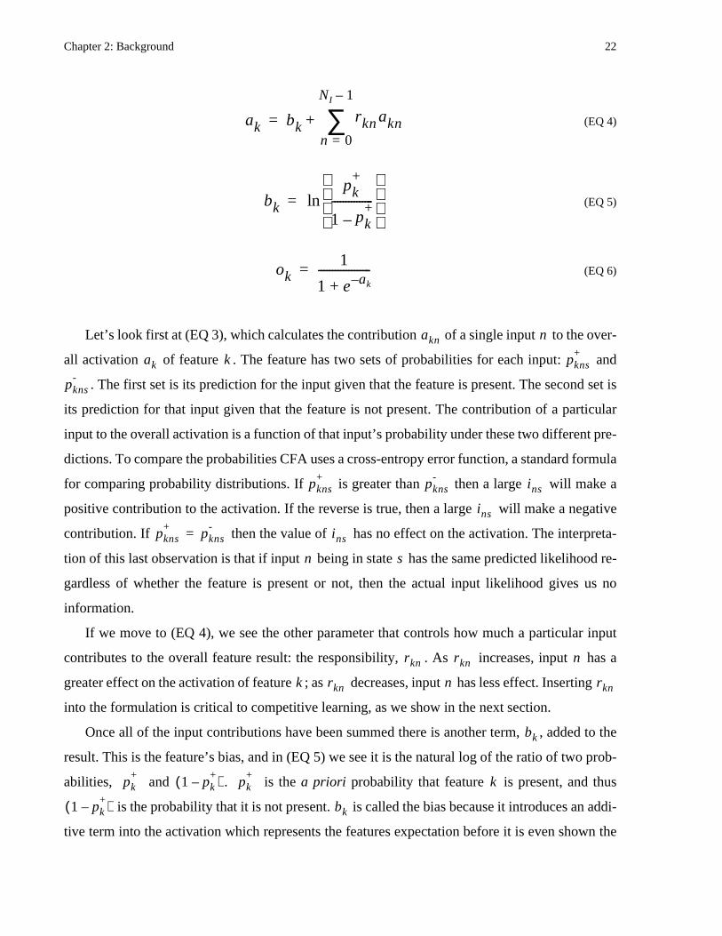
(EQ 4)
(EQ 5)
(EQ 6)
Let’s look first at (EQ 3), which calculates the contribution of a single input to the over-
all activation of feature . The feature has two sets of probabilities for each input: and
. The first set is its prediction for the input given that the feature is present. The second set is
its prediction for that input given that the feature is not present. The contribution of a particular
input to the overall activation is a function of that input’s probability under these two different pre-
dictions. To compare the probabilities CFA uses a cross-entropy error function, a standard formula
for comparing probability distributions. If is greater than then a large will make a
positive contribution to the activation. If the reverse is true, then a large will make a negative
contribution. If then the value of has no effect on the activation. The interpreta-
tion of this last observation is that if input being in state has the same predicted likelihood re-
gardless of whether the feature is present or not, then the actual input likelihood gives us no
information.
If we move to (EQ 4), we see the other parameter that controls how much a particular input
contributes to the overall feature result: the responsibility, . As increases, input has a
greater effect on the activation of feature ; as decreases, input has less effect. Inserting
into the formulation is critical to competitive learning, as we show in the next section.
Once all of the input contributions have been summed there is another term, , added to the
result. This is the feature’s bias, and in (EQ 5) we see it is the natural log of the ratio of two prob-
abilities, and . is the a priori probability that feature is present, and thus
is the probability that it is not present. is called the bias because it introduces an addi-
tive term into the activation which represents the features expectation before it is even shown the
ak bkrkn akn
n 0=
NI 1–
∑+=
bk
pk+
1 pk+
–---------------
ln=
ok1
1 e ak–+-------------------=
akn n
ak k pkns+
pkns-
pkns+
pkns-
ins
ins
pkns+
pkns-
= ins
n s
rkn rkn n
k rkn n rkn
bk
pk+
1 p– k+( ) pk
+k
1 p– k+( ) bk

Chapter 2: Background 23
input. If is greater than 0.5, then this term will be positive; if it is less, this term will be neg-
ative. If it is equally likely that the feature is present or not present, then the bias will be zero.
The activation has a possible range from negative infinity to positive infinity. We need to
use this value to generate a probability between zero and one. Given our derivation so far, the
meaningful way to do this, in a probabilistic sense, is to use the sigmoid activation function given
in (EQ 6).
Input Reconstruction and Competitive Learning
During learning, the current CFA model is iteratively presented with an image from the training
set and then adjusted to better account for the image contents. Each of these iterations has two stag-
es: a detection stage, which was discussed above, and a reconstruction and learning stage. During
the detection stage all of the features calculate their outputs. The resulting ensemble of feature out-
puts can be viewed as a coding of the input image in terms of the patterns it contains. To determine
how accurate this coding is, it is used as the input to a reconstruction stage in which the pattern
models contained in the features are combined to produce a prediction of the original input. A fea-
ture can be used to predict a set of state probabilities for each of its inputs by making the best guess
possible: that the probability set for an input is identical to its associated set in the pattern model.
The extent to which a feature’s model contributes to the reconstruction of a particular input is a
function of two factors. The first is the probability produced by the feature during the detection
stage, which is now part of the coding, and the second is the responsibility of the feature, , for
that input. As each of these increases, so does the influence of the feature’s predictions on the value
of the input in the reconstruction.
Once the reconstruction stage is complete, the error between the predictions of the features and
the original image is calculated. The precise value of this error is not important, however; what is
important is knowing how the CFA model can be changed to lower the error. A standard way of
doing this is to calculate the partial derivatives of the error function with respect to the each of the
model parameters. Learning consists of evaluating the value of these derivatives during training
and adjusting the model parameters by an amount proportional to their effect on the error. This is
not precise since we only have the individual partial derivatives, but it has been shown to work well
in many other learning algorithms.
A good way to evaluate how a learning method will behave is to look at its partial derivatives
with respect to critical parameters and see what sorts of conditions will cause these parameters to
pk+
ak
rkn

Chapter 2: Background 24
increase or decrease. The most important feature parameters for competitive learning are the re-
sponsibilities, , we introduced in a previous section, which control the extent to which a feature
considers a particular input to be part of its pattern. Below we show the simplified partial derivative
of the model error with respect to the responsibility of feature for input , , where
• is the total error over the entire input set I
• is the error on input considering the ensemble of features
• is the error on input considering feature alone
• is the number of inputs in the data set
• , , and are additional factors which are outside the scope of this discussion
(EQ 7)
If this derivative is negative, it indicates that raising will lower the total error; if it is posi-
tive, lowering will lower the total error. The most important and influential term in (EQ 7) is
, which occurs twice weighted by the current responsibility. If feature more accurate-
ly predicts input than does the ensemble of features, the value of the term will be negative. If the
opposite is true, it will be positive. The first instance of this term has a straightforward effect: if
feature is more accurate than the ensemble with respect to input then is encouraged to
increase. The second instance of this term is more subtle. The summation in brackets is a weighted
sum over all inputs of the error difference term. If this sum is negative it indicates in essence that
feature should consider itself to be present in the input, as this would lower the total error. If
is positive, increasing will increase the feature’s output and thus will cause the feature to con-
sider itself more likely to be present.
What all of the above shows is that in CFA the adjustment of critical feature parameters during
learning is inextricably linked with the performance of that feature relative to any other features
that are trying to use the same inputs. When the ensemble is presented with a training example, the
feature that most accurately predicts a given input will end up with increased responsibility for that
input. A feature which predicts an input with much less accuracy than others will receive reduced
responsibility for that input. Over time, features will become localized to the patterns they predict
rkn
k n rkn
EI
En n
Ekn n k
ND
C1 C2 C3
EI∂rkn∂
---------- C1rkn Ekn En–( ) akn C2rkm Ekm Em–( )
m 0=
ND 1–
∑
C3+ +=
rkn
rkn
Ekn En–( ) k
n
k n rkn
k akn
rkn

Chapter 2: Background 25
best.
A side effect of the competitive formulation is that it provides an elegant way to include non-
target training examples in the training set. If one is using an unsupervised learning method the
training set typically can include only examples of the target class. Unsupervised learning methods
focus almost exclusively on representation of the training set, and so would attempt to represent
target and non-target examples alike if both were present. Since the method only sees target exam-
ples it has no opportunity to model the appearance of difficult non-target objects. CFA allows non-
target examples by introducing the presence of a “virtual” ensemble of features that have both very
low error and high responsibility for all inputs when a non-target example is presented. These fea-
tures do not actually exist, in that they are never explicitly instantiated, but their virtual presence
effectively lowers for each input . Learning proceeds as if features existed that performed
well on non-target images, so from the perspective of all of the actual features there are now others
which outperform them on these images. Competitive learning forces the actual features to refine
their expectations such that they are less likely to detect non-target objects in the future. Using vir-
tual features and non-target examples helps to ensure that features are detecting patterns that are
characteristic of the target class in particular. The combination of unsupervised learning techniques
together with the use of non-target training examples places CFA between the supervised and un-
supervised learning camps. It is probably most accurate to call CFA a semi-supervised method.
One of the critical attributes of CFA learning is that it couples detection and representation. In
CFA, representation is accomplished by the ensemble of features predicting the state of an input.
If a feature does not consider itself to be present in an example, it does not attempt to predict the
state of any inputs. If a feature does not accurately predict a pattern, other features will assume re-
sponsibility for detecting that pattern via competitive learning. Thus features must both detect and
represent patterns accurately.
Building Hierarchies
We have discussed how competitive learning encourages features to decompose the input into
independent, characteristic patterns. The other goal is to use the same mechanism to build hierar-
chies of higher-level features that represent the likely arrangements of those patterns. In order to
build feature hierarchies we must be able to use the output of one feature as the input of another.
Feature outputs are binomial in that a feature is either present or not present; is the probability
that the feature is present, so is the probability that it is not. A feature output thus has the
En n
ok
1 ok–( )

Chapter 2: Background 26
proper probabilistic meaning to be used as another feature’s input. The output value is also a non-
linear function of the inputs , which is critical as otherwise the rule of linear superposition
would apply. Superposition states that any multi-layer hierarchy of linear operations is equivalent
to some single linear operation, making hierarchy pointless.
Summary
The CFA learning method is designed to both automatically decompose the input space into
separate characteristic patterns and automatically build hierarchies to unify these patterns. Decom-
position is achieved via competitive learning between separate pattern detectors called features.
Hierarchies are built by using multiple layers of features, with each layer trained on the output of
the previous. CFA encourages features to detect patterns which are highly characteristic of the tar-
get class through the combination of a semi-supervised learning approach with a strong coupling
between detection and representation.
2.4 Programmable HardwareA Programmable Logic Device (PLD) is a chip which in some fashion allows a user to control
the logic functions it implements. There are many types of PLDs, and these have found use in a
wide range of applications[23]. When compared to custom hardware, the advantages of PLDs are
shorter design cycles and the ability to re-program existing systems if a change in functionality is
required. The chief disadvantages are a significant speed penalty (approximately 66-75% speed re-
duction) and greater cost in volume. When compared to a software implementation the advantage
of programmable hardware is the potential for a significant speed increase, and the major disad-
vantage is a longer design cycle. For designs that are too large to fit on a single PLD, programmable
systems comprised of a set of interconnected PLDs are used. In this section we present an overview
of one type of PLD, the Field Programmable Gate Array (FPGA), followed by a basic discussion
of programmable systems. We end with a description of the programmable system used in this
work: the Transmogrifier-2a (TM-2a).
2.4.1 Field Programmable Gate Arrays (FPGAs)Field-Programmable Gate Arrays are one of the most popular types of PLDs today. An FPGA
ins{ }
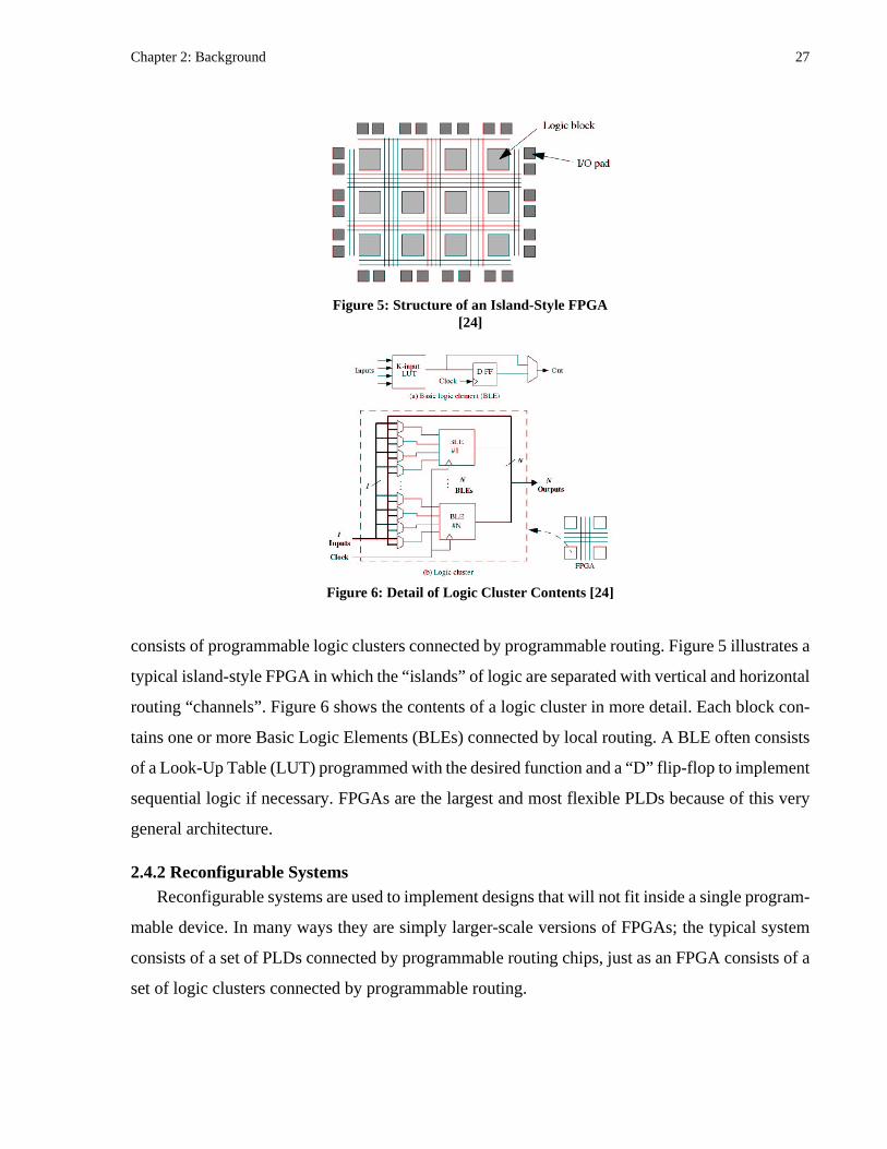
Chapter 2: Background 27
consists of programmable logic clusters connected by programmable routing. Figure 5 illustrates a
typical island-style FPGA in which the “islands” of logic are separated with vertical and horizontal
routing “channels”. Figure 6 shows the contents of a logic cluster in more detail. Each block con-
tains one or more Basic Logic Elements (BLEs) connected by local routing. A BLE often consists
of a Look-Up Table (LUT) programmed with the desired function and a “D” flip-flop to implement
sequential logic if necessary. FPGAs are the largest and most flexible PLDs because of this very
general architecture.
2.4.2 Reconfigurable SystemsReconfigurable systems are used to implement designs that will not fit inside a single program-
mable device. In many ways they are simply larger-scale versions of FPGAs; the typical system
consists of a set of PLDs connected by programmable routing chips, just as an FPGA consists of a
set of logic clusters connected by programmable routing.
Figure 5: Structure of an Island-Style FPGA [24]
Figure 6: Detail of Logic Cluster Contents [24]

Chapter 2: Background 28
2.4.3 The TM-2a Reconfigurable SystemThe Transmogrifier-2a [18][19] is an extensible programmable hardware architecture contain-
ing from one to sixteen boards in power-of-two increments. Each board contains two Altera
10K100 FPGAs [29], four I-Cube IQ320 Field Programmable Interconnect Devices (FPIDs) for
inter-chip and inter-board routing, 8 MB of SRAM in four independent banks, and other house-
keeping and programmable clocking circuitry. Its major uses are as a fast prototyping tool for large
hardware designs and as a platform for reconfigurable computing research [20][21][22]. In addi-
tion, the circuits produced are large enough to provide critical benchmarks for ongoing research
into next-generation FPGA architectures.
In this project we use a 16-board system. Video input and output cards are attached to I/O con-
nectors on two of the boards. This allows the image data to be read directly from the camera and
face detection results to be displayed on an attached monitor with no need for an intervening com-
puter. The system clock frequency is set at 12.5 MHz; this is the highest frequency at which the
SRAM operates reliably.
The Altera 10K100
As mentioned above, the TM-2a uses Altera 10K100 FPGAs [29]. These FPGAs are similar in
structure to the generic FPGA presented in Section 2.4.1. Each contains 4992 Logic Cells (LCs),
which are essentially equivalent to one of the BLEs described earlier. In addition, a 10K100 con-
tains 24,576 bits of on-chip memory in 12 independent 2048-bit banks. Each bank may be sepa-
rately configured to be 1, 2, 4, or 8 bits wide.
2.5 Object Detection Using Reconfigurable SystemsIt is instructive to look at tasks similar to face detection that have been implemented using re-
configurable hardware. To our knowledge there is no hardware system, reconfigurable or other-
wise, which performs face detection, but there are systems designed to perform other object
detection tasks. In this section we review two approaches to Automated Target Recognition (ATR)
on Synthetic Aperture Radar (SAR) data which have been implemented on reconfigurable systems.
2.5.1 ATR Problem DescriptionAlthough ATR uses the term “recognition”, by our earlier definition we would consider this to
be a detection task and it bears many resemblances to standard visual detection problems. The SAR
input data is very similar to a greyscale image where intensity indicates radar reflectance rather
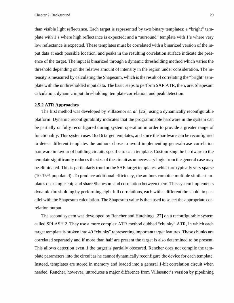
Chapter 2: Background 29
than visible light reflectance. Each target is represented by two binary templates: a “bright” tem-
plate with 1’s where high reflectance is expected; and a “surround” template with 1’s where very
low reflectance is expected. These templates must be correlated with a binarized version of the in-
put data at each possible location, and peaks in the resulting correlation surface indicate the pres-
ence of the target. The input is binarized through a dynamic thresholding method which varies the
threshold depending on the relative amount of intensity in the region under consideration. The in-
tensity is measured by calculating the Shapesum, which is the result of correlating the “bright” tem-
plate with the unthresholded input data. The basic steps to perform SAR ATR, then, are: Shapesum
calculation, dynamic input thresholding, template correlation, and peak detection.
2.5.2 ATR ApproachesThe first method was developed by Villasenor et. al. [26], using a dynamically reconfigurable
platform. Dynamic reconfigurability indicates that the programmable hardware in the system can
be partially or fully reconfigured during system operation in order to provide a greater range of
functionality. This system uses 16x16 target templates, and since the hardware can be reconfigured
to detect different templates the authors chose to avoid implementing general-case correlation
hardware in favour of building circuits specific to each template. Customizing the hardware to the
template significantly reduces the size of the circuit as unnecessary logic from the general case may
be eliminated. This is particularly true for the SAR target templates, which are typically very sparse
(10-15% populated). To produce additional efficiency, the authors combine multiple similar tem-
plates on a single chip and share Shapesum and correlation between them. This system implements
dynamic thresholding by performing eight full correlations, each with a different threshold, in par-
allel with the Shapesum calculation. The Shapesum value is then used to select the appropriate cor-
relation output.
The second system was developed by Rencher and Hutchings [27] on a reconfigurable system
called SPLASH 2. They use a more complex ATR method dubbed “chunky” ATR, in which each
target template is broken into 40 “chunks” representing important target features. These chunks are
correlated separately and if more than half are present the target is also determined to be present.
This allows detection even if the target is partially obscured. Rencher does not compile the tem-
plate parameters into the circuit as he cannot dynamically reconfigure the device for each template.
Instead, templates are stored in memory and loaded into a general 1-bit correlation circuit when
needed. Rencher, however, introduces a major difference from Villasenor’s version by pipelining
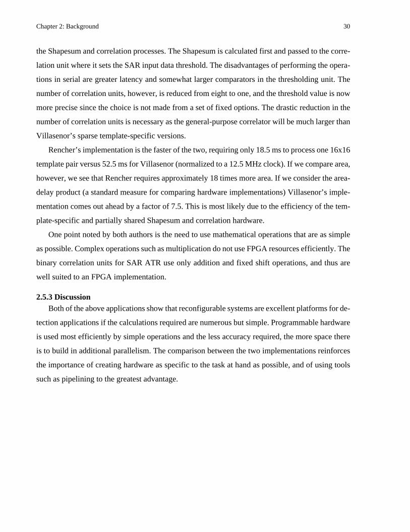
Chapter 2: Background 30
the Shapesum and correlation processes. The Shapesum is calculated first and passed to the corre-
lation unit where it sets the SAR input data threshold. The disadvantages of performing the opera-
tions in serial are greater latency and somewhat larger comparators in the thresholding unit. The
number of correlation units, however, is reduced from eight to one, and the threshold value is now
more precise since the choice is not made from a set of fixed options. The drastic reduction in the
number of correlation units is necessary as the general-purpose correlator will be much larger than
Villasenor’s sparse template-specific versions.
Rencher’s implementation is the faster of the two, requiring only 18.5 ms to process one 16x16
template pair versus 52.5 ms for Villasenor (normalized to a 12.5 MHz clock). If we compare area,
however, we see that Rencher requires approximately 18 times more area. If we consider the area-
delay product (a standard measure for comparing hardware implementations) Villasenor’s imple-
mentation comes out ahead by a factor of 7.5. This is most likely due to the efficiency of the tem-
plate-specific and partially shared Shapesum and correlation hardware.
One point noted by both authors is the need to use mathematical operations that are as simple
as possible. Complex operations such as multiplication do not use FPGA resources efficiently. The
binary correlation units for SAR ATR use only addition and fixed shift operations, and thus are
well suited to an FPGA implementation.
2.5.3 DiscussionBoth of the above applications show that reconfigurable systems are excellent platforms for de-
tection applications if the calculations required are numerous but simple. Programmable hardware
is used most efficiently by simple operations and the less accuracy required, the more space there
is to build in additional parallelism. The comparison between the two implementations reinforces
the importance of creating hardware as specific to the task at hand as possible, and of using tools
such as pipelining to the greatest advantage.
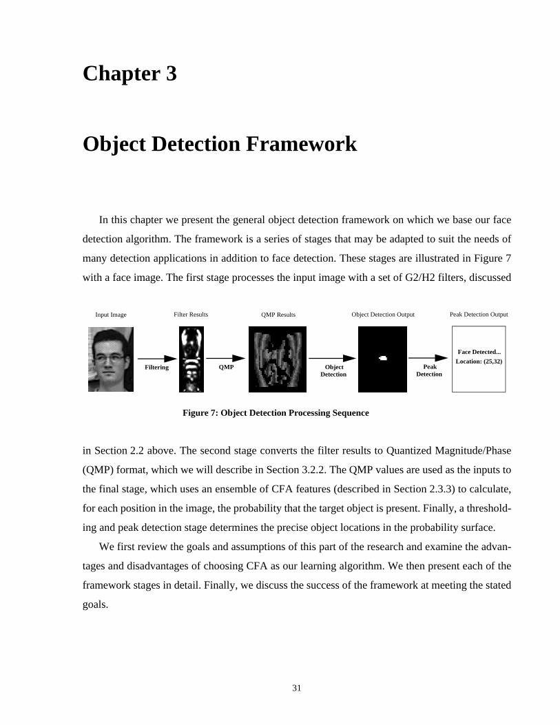
31
Chapter 3
Object Detection Framework
In this chapter we present the general object detection framework on which we base our face
detection algorithm. The framework is a series of stages that may be adapted to suit the needs of
many detection applications in addition to face detection. These stages are illustrated in Figure 7
with a face image. The first stage processes the input image with a set of G2/H2 filters, discussed
in Section 2.2 above. The second stage converts the filter results to Quantized Magnitude/Phase
(QMP) format, which we will describe in Section 3.2.2. The QMP values are used as the inputs to
the final stage, which uses an ensemble of CFA features (described in Section 2.3.3) to calculate,
for each position in the image, the probability that the target object is present. Finally, a threshold-
ing and peak detection stage determines the precise object locations in the probability surface.
We first review the goals and assumptions of this part of the research and examine the advan-
tages and disadvantages of choosing CFA as our learning algorithm. We then present each of the
framework stages in detail. Finally, we discuss the success of the framework at meeting the stated
goals.
Figure 7: Object Detection Processing Sequence
Input Image Filter Results QMP Results Object Detection Output
Filtering QMP ObjectDetection
Peak Detection Output
PeakDetection
Face Detected...
Location: (25,32)

Chapter 3: Object Detection Framework 32
3.1 Goals and AssumptionsIn developing a general object detection framework, our goal was to provide a software suite
that we could use to develop the face detection application and which could also be used to develop
detection applications for a variety of target objects. We chose this general approach for two rea-
sons: because it extends the applicability of the work beyond the single case of face detection; and
because it helps to ensure that face-specific human biases have minimal influence on the choice of
detection strategy. To support a range of objects the processing stages are highly parameterized,
since each particular application will require different types of information at different levels of
accuracy.
We assume that significant variation in object scale and in-plane rotation will be handled out-
side of the framework by scaling or rotating the input image. The amount of variation that can be
handled within the framework will depend on the object’s appearance and on the training set used.
3.2 Image ProcessingThe first two stages in the framework process the incoming image and convert it to a format
suitable for use with CFA. The image is convolved with a bank of oriented and scaled G2/H2 fil-
ters, and then the filter results are converted to Quantized Magnitude/Phase (QMP) representation.
In this section we present the details of these steps and how they affect the framework as a whole.
3.2.1 G2/H2 FilteringThe first processing step is to apply a set of oriented and scaled G2/H2 filters. The precise ori-
entations and scales used will depend on the application in question, but in general these will be
chosen such that they capture important structure in the target object. We chose this filtering meth-
od because of the need to resolve a set of interrelated problems caused by the assumption of un-
controlled lighting, by the choice of learning algorithm, and by the goal of an efficient hardware
implementation. Assuming uncontrolled lighting implies that the intensity value of any individual
pixel has little meaning, as changes in lighting brightness and direction could cause it to vary con-
siderably. CFA requires that the algorithm inputs are in the form of probabilities, which, in con-
trast, must have very well-defined meanings. This makes raw pixel intensity values unsuitable as
direct inputs to CFA. We must ensure in addition that any image processing we do may be imple-
mented efficiently in hardware, or otherwise we will violate one of the primary goals of this re-
search. While G2/H2 filtering does not solve all of these problems, it does begin to address them.
Chapter 3: Object Detection Framework 33
The filters have no DC response, making them insensitive to additive scalar lighting changes, or
lighting brightness. At each location they analyze the intensity variation over a local set of pixels
to derive texture information that is much more meaningful than a single intensity alone. The G2/
H2 filters, as we discuss in Chapter 2, are also very efficient due to the combined properties of X-
Y separability and orientation-steerability.
3.2.2 QMP ConversionWhile the individual filter results now have more meaning than individual pixels, they are not
the probabilities required as inputs to CFA. To produce these probabilities we convert each G2/H2
response to a format that we designed to preserve the important information in each filter result and
to be both calculated and stored efficiently. This format is called Quantized Magnitude/Phase
(QMP) format. It is important to note that this choice of representation is a crucial factor in the ef-
ficiency of the final hardware implementation.
In order to discuss how QMP works, we must introduce the concept of filter response phase
and magnitude. G2 and H2 are a quadrature pair, which means that in the frequency domain the
phase response of H2 is shifted 90 degrees with respect to G2. This relationship produces an inter-
esting property: we can use a linear combination of G2 and H2 to create a filter with the same mag-
nitude response but arbitrary frequency phase shift. If we apply both filters at a given location in
an image, we can use the two responses to determine the filter phase which would receive the stron-
gest response magnitude. This is often simply called the phase of the response. Response phase is
a useful description of local image texture that is invariant with respect to multiplicative changes
in lighting, or lighting contrast. Magnitude is not completely irrelevant, however, since in smooth
areas of the image the filter response will be too weak for phase to be meaningful, and we need to
detect this condition. The phase and magnitude of the G2/H2 response are calculated simply as:
(EQ 8)
(EQ 9)
G2/H2 G2 H2+=
Φ G2/H2( ) HG----
atan=

Chapter 3: Object Detection Framework 34
This is illustrated graphically in Figure 8.
The key to QMP is combining phase and magnitude in-
formation in a way that is compact, computationally cheap
to calculate, and, when combined with the CFA object clas-
sifier, makes detection extremely efficient. While we know
the phase angle provides useful information, it is unclear
how the actual value should be calculated and used. From a
hardware perspective an accurate phase value is expensive
to represent and even more expensive to calculate, as it
would involve evaluating the computationally complex function . Instead we divide
the phase space into a set of bins. A response phase angle can now be encoded using only the bin
number into which it falls. If there are phase bins and is divisible by four (to ensure the same
number of bins in each quadrant), the calculation of the correct bin in hardware may be accom-
plished with two absolute value operations, constant multiplications, compare op-
erations, and minimal additional logic to evaluate the signs of the G2/H2 responses and adjust the
bin number appropriately. The number of bins required depends on the accuracy needed by the ap-
plication.
To incorporate magnitude information we add an extra “bin” to represent the case when the re-
sponse is below a fixed threshold. Although this means that the framework will not detect a target
object with extremely low contrast, these cases should be both rare and unimportant. Calculating
the vector’s magnitude requires squaring both the G2 and H2 responses. If either G2 or H2 alone
is greater than or equal to the threshold, however, there is no need to perform the calculation. We
will only need to provide a multiplier large enough to square the bits representing values below the
threshold.
Using the QMP representation is critical to hardware efficiency. Once calculated, the QMP val-
ue is very compact. If there are there are phase bins plus one low-magnitude bin, we only need
ceil(log2(n+1)) bits to store each result. In an application that used eight bins of phase accuracy,
we would only need four bits per QMP value. This is a savings of 12 bits from the storage required
for the G2/H2 pair used to derive the QMP value. QMP is also an efficient input to CFA. As we
will discuss in Chapter 5, quantizing the filter output into one of a set of bins removes the need for
any multiplications in the face classifier network.
Figure 8: G2/H2 Phase and Magnitude Calculation
G2 Response
H2 Response
(G,H)
Phase
Mag
nitud
e
H G⁄( )atan
n n
n4---
2–n4---
1–
n
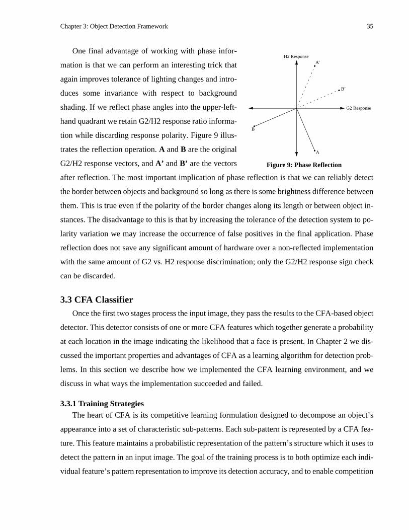
Chapter 3: Object Detection Framework 35
One final advantage of working with phase infor-
mation is that we can perform an interesting trick that
again improves tolerance of lighting changes and intro-
duces some invariance with respect to background
shading. If we reflect phase angles into the upper-left-
hand quadrant we retain G2/H2 response ratio informa-
tion while discarding response polarity. Figure 9 illus-
trates the reflection operation. A and B are the original
G2/H2 response vectors, and A’ and B’ are the vectors
after reflection. The most important implication of phase reflection is that we can reliably detect
the border between objects and background so long as there is some brightness difference between
them. This is true even if the polarity of the border changes along its length or between object in-
stances. The disadvantage to this is that by increasing the tolerance of the detection system to po-
larity variation we may increase the occurrence of false positives in the final application. Phase
reflection does not save any significant amount of hardware over a non-reflected implementation
with the same amount of G2 vs. H2 response discrimination; only the G2/H2 response sign check
can be discarded.
3.3 CFA ClassifierOnce the first two stages process the input image, they pass the results to the CFA-based object
detector. This detector consists of one or more CFA features which together generate a probability
at each location in the image indicating the likelihood that a face is present. In Chapter 2 we dis-
cussed the important properties and advantages of CFA as a learning algorithm for detection prob-
lems. In this section we describe how we implemented the CFA learning environment, and we
discuss in what ways the implementation succeeded and failed.
3.3.1 Training StrategiesThe heart of CFA is its competitive learning formulation designed to decompose an object’s
appearance into a set of characteristic sub-patterns. Each sub-pattern is represented by a CFA fea-
ture. This feature maintains a probabilistic representation of the pattern’s structure which it uses to
detect the pattern in an input image. The goal of the training process is to both optimize each indi-
vidual feature’s pattern representation to improve its detection accuracy, and to enable competition
G2 Response
H2 ResponseA’
A
B’
B
Figure 9: Phase Reflection

Chapter 3: Object Detection Framework 36
between features to determine the optimal number and scope of sub-patterns. In this section we dis-
cuss three aspects of our CFA training implementation that enhance its flexibility, accuracy, power,
and feasibility.
Improving Flexibility and Accuracy
In the most straightforward implementation of CFA, all of the training set images would be the
same size and would be cropped such that the target object is always in same position. This is a
common approach for many learning algorithms, both unsupervised and supervised, because it
greatly simplifies the training process. We have developed an alternate implementation that struc-
tures the CFA learning environment to allow any image size or object position, and in the process
promotes greater detection accuracy.
When an input image is presented to the algorithm we create multiple copies of the existing
features such that there is one copy of each feature located at each position in the image. We call
this process feature replication. Patterns will be detected regardless of their position, since every
feature has a copy at every image location. Even though the all of the copies of a given feature are
identical, however, they are considered separate for the purposes of competitive learning. All fea-
ture copies, regardless of which original feature they were copied from, will compete with each
other to detect and represent the input just as separate features would. As parameter updates are
calculated, all changes that apply to a feature’s copies are summed and applied to the original fea-
ture. Readers familiar with neural networks will recognize this as similar to weight sharing, with
the notable exception that the effective number of neurons changes with the image dimensions.
Feature replication has three major implications. It allows us to use images of any size as input
since the number of feature copies can change with the image dimensions. It also allows us to use
images containing any number of target objects appearing at any position and allows patterns rep-
resented by different features to move with respect to one another with no constraints. Lastly, it
promotes detection accuracy. Consider that copies of the same feature located near each other will
be using many of the same inputs. If a characteristic pattern is present, many of the copies around
its location will likely respond, creating a peak in the feature result surface. Competitive learning
will encourage the more successful copies to have a greater response while suppressing the others.
As learning proceeds, the response peak will narrow and heighten; narrower, higher peaks result
in more accurate detection.

Chapter 3: Object Detection Framework 37
Enabling Multi-Feature Training
While the CFA formulation allows any number of separate competing features, it does not
specify how to determine how many features are required. One good option would be to perform
multiple training runs, each with a different number of features, and statistically analyze the results
to determine the optimum number. In practice, however, we found that if we simply began training
with multiple concurrent features, the feature that first started to detect a pattern immediately pre-
vented the others from learning anything. To work around this problem we implemented an itera-
tive method for adding and removing features.
Figure 10 describes this process in pseudocode. In each iteration we first “freeze” any existing
features, meaning that we fix their parameters and do not allow them to learn. We then create a new
randomly initialized feature. We train this feature by itself on data weighted to emphasize areas on
which the current ensemble has the greatest error. We train this feature until it has learned a pattern
reasonably well, which we evaluate by recording the feature’s maximum output. Assuming the
new feature is not the very first to be added, we then un-freeze the whole ensemble and train them
together competitively. As we proceed through the training set we keep track of the maximum re-
sponse each feature produces. If the maximum response for a feature over the set is below a given
threshold, we assume that it has been forced from its pattern by another feature and should be re-
moved. We continue to train until either we have removed a feature or have made a fixed number
DO{
“freeze” all existing feature parameterscreate new featuretrain the new feature on weighted data until it learns a pattern reasonably welladd new feature to existing features and “unfreeze”
IF(more than one feature){
“unfreeze” all features
DO{
train once through entire training setcheck if we should remove any features
}UNTIL(we reach a fixed number of iterations or we remove a feature)}
}UNTIL(we have removed a feature N iterations in a row)
Figure 10: Pseudocode for Iterative Feature Addition/Removal

Chapter 3: Object Detection Framework 38
of passes through the training set. We then attempt to add another feature. The process is repeated
until we remove a feature in each of a number of successive iterations. The precise number of iter-
ations is another parameter to the process.
This iterative method has two major drawbacks. First, it is prone to becoming trapped in local
minima that are found while training with a small number of features, and that cannot be escaped
by adding more. Second, it introduces several additional training parameters which have no a pri-
ori reasonable values and yet can have significant effects on the final result. Nonetheless, it pro-
vides a reasonable solution to the problem of determining the number of features, given that we
cannot simply train multiple features from scratch. As we discuss in the testing section below, we
were able to find settings with which this method correctly determined the number of features for
an artificial test data with two independent patterns.
Modifying Feature Scope
The CFA formulation assumes that every feature has some prediction for every input. This is
not feasible in an implementation, however, as we must limit the scope of a feature in order to store
its parameters in a reasonable amount of space and evaluate its results in a reasonable amount of
time. In this implementation, each feature has a current scope defined by a rectangular area. For
good efficiency we would like to limit the scope of a feature to the minimum rectangle required to
encompass its characteristic pattern. On the other hand, to perform flexible learning we would like
to make sure that no characteristic pattern is truncated by a feature’s scope. We need to be able to
both shrink the scope of features that are much larger than their pattern and increase the scope of
features if the patterns are currently being truncated
To do this we periodically examine each feature during training. If all the feature’s effective
“weights” along one edge of the scope rectangle are vanishingly small, then the connections along
that edge are removed and the feature shrinks. If there is a weight along an edge that is larger than
a given threshold we assume that the pattern could be extended in that direction and we add a set
of connections to that edge of the scope. In this way the scope of a feature will adjust to the scope
of its pattern during learning. This method performed well during testing, as described in Section
3.3.3 below.
3.3.2 HierarchyIf an object is decomposed into multiple features, then hierarchy needs to be built to unify the
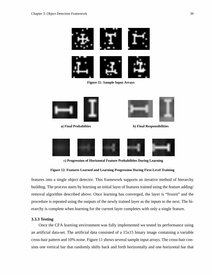
Chapter 3: Object Detection Framework 39
features into a single object detector. This framework supports an iterative method of hierarchy
building. The process starts by learning an initial layer of features trained using the feature adding/
removal algorithm described above. Once learning has converged, the layer is “frozen” and the
procedure is repeated using the outputs of the newly trained layer as the inputs to the next. The hi-
erarchy is complete when learning for the current layer completes with only a single feature.
3.3.3 Testing Once the CFA learning environment was fully implemented we tested its performance using
an artificial data-set. The artificial data consisted of a 15x15 binary image containing a variable
cross-hair pattern and 10% noise. Figure 11 shows several sample input arrays. The cross-hair con-
sists one vertical bar that randomly shifts back and forth horizontally and one horizontal bar that
Figure 11: Sample Input Arrays
Figure 12: Features Learned and Learning Progression During First-Level Training
a) Final Probabilties b) Final Responsibilities
c) Progression of Horizontal Feature Probabilities During Learning
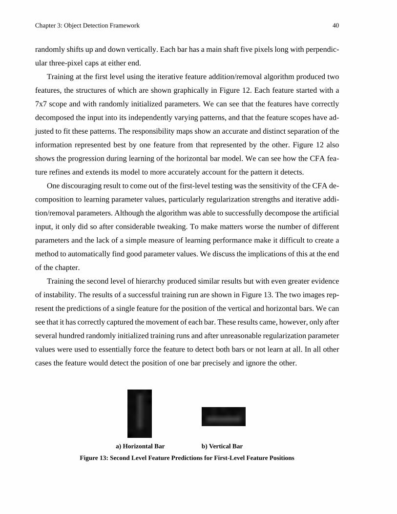
Chapter 3: Object Detection Framework 40
randomly shifts up and down vertically. Each bar has a main shaft five pixels long with perpendic-
ular three-pixel caps at either end.
Training at the first level using the iterative feature addition/removal algorithm produced two
features, the structures of which are shown graphically in Figure 12. Each feature started with a
7x7 scope and with randomly initialized parameters. We can see that the features have correctly
decomposed the input into its independently varying patterns, and that the feature scopes have ad-
justed to fit these patterns. The responsibility maps show an accurate and distinct separation of the
information represented best by one feature from that represented by the other. Figure 12 also
shows the progression during learning of the horizontal bar model. We can see how the CFA fea-
ture refines and extends its model to more accurately account for the pattern it detects.
One discouraging result to come out of the first-level testing was the sensitivity of the CFA de-
composition to learning parameter values, particularly regularization strengths and iterative addi-
tion/removal parameters. Although the algorithm was able to successfully decompose the artificial
input, it only did so after considerable tweaking. To make matters worse the number of different
parameters and the lack of a simple measure of learning performance make it difficult to create a
method to automatically find good parameter values. We discuss the implications of this at the end
of the chapter.
Training the second level of hierarchy produced similar results but with even greater evidence
of instability. The results of a successful training run are shown in Figure 13. The two images rep-
resent the predictions of a single feature for the position of the vertical and horizontal bars. We can
see that it has correctly captured the movement of each bar. These results came, however, only after
several hundred randomly initialized training runs and after unreasonable regularization parameter
values were used to essentially force the feature to detect both bars or not learn at all. In all other
cases the feature would detect the position of one bar precisely and ignore the other.
Figure 13: Second Level Feature Predictions for First-Level Feature Positions
a) Horizontal Bar b) Vertical Bar
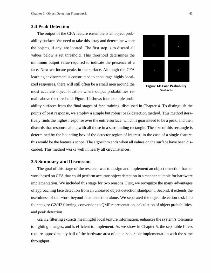
Chapter 3: Object Detection Framework 41
3.4 Peak DetectionThe output of the CFA feature ensemble is an object prob-
ability surface. We need to take this array and determine where
the objects, if any, are located. The first step is to discard all
values below a set threshold. This threshold determines the
minimum output value required to indicate the presence of a
face. Next we locate peaks in the surface. Although the CFA
learning environment is constructed to encourage highly local-
ized responses, there will still often be a small area around the
most accurate object location where output probabilities re-
main above the threshold. Figure 14 shows four example prob-
ability surfaces from the final stages of face training, discussed in Chapter 4. To distinguish the
points of best response, we employ a simple but robust peak detection method. This method itera-
tively finds the highest response over the entire surface, which is guaranteed to be a peak, and then
discards that response along with all those in a surrounding rectangle. The size of this rectangle is
determined by the bounding box of the detector region of interest; in the case of a single feature,
this would be the feature’s scope. The algorithm ends when all values on the surface have been dis-
carded. This method works well in nearly all circumstances.
3.5 Summary and DiscussionThe goal of this stage of the research was to design and implement an object detection frame-
work based on CFA that could perform accurate object detection in a manner suitable for hardware
implementation. We included this stage for two reasons. First, we recognize the many advantages
of approaching face detection from an unbiased object detection standpoint. Second, it extends the
usefulness of our work beyond face detection alone. We separated the object detection task into
four stages: G2/H2 filtering, conversion to QMP representation, calculation of object probabilities,
and peak detection.
G2/H2 filtering extracts meaningful local texture information, enhances the system’s tolerance
to lighting changes, and is efficient to implement. As we show in Chapter 5, the separable filters
require approximately half of the hardware area of a non-separable implementation with the same
throughput.
Figure 14: Face Probability Surfaces
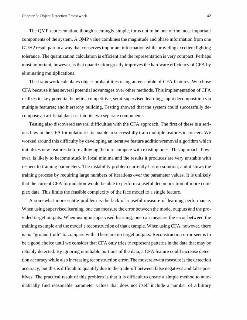
Chapter 3: Object Detection Framework 42
The QMP representation, though seemingly simple, turns out to be one of the most important
components of the system. A QMP value combines the magnitude and phase information from one
G2/H2 result pair in a way that conserves important information while providing excellent lighting
tolerance. The quantization calculation is efficient and the representation is very compact. Perhaps
most important, however, is that quantization greatly improves the hardware efficiency of CFA by
eliminating multiplications.
The framework calculates object probabilities using an ensemble of CFA features. We chose
CFA because it has several potential advantages over other methods. This implementation of CFA
realizes its key potential benefits: competitive, semi-supervised learning; input decomposition via
multiple features; and hierarchy building. Testing showed that the system could successfully de-
compose an artificial data-set into its two separate components.
Testing also discovered several difficulties with the CFA approach. The first of these is a seri-
ous flaw in the CFA formulation: it is unable to successfully train multiple features in concert. We
worked around this difficulty by developing an iterative feature addition/removal algorithm which
initializes new features before allowing them to compete with existing ones. This approach, how-
ever, is likely to become stuck in local minima and the results it produces are very unstable with
respect to training parameters. The instability problem currently has no solution, and it slows the
training process by requiring large numbers of iterations over the parameter values. It is unlikely
that the current CFA formulation would be able to perform a useful decomposition of more com-
plex data. This limits the feasible complexity of the face model to a single feature.
A somewhat more subtle problem is the lack of a useful measure of learning performance.
When using supervised learning, one can measure the error between the model outputs and the pro-
vided target outputs. When using unsupervised learning, one can measure the error between the
training example and the model’s reconstruction of that example. When using CFA, however, there
is no “ground truth” to compare with. There are no target outputs. Reconstruction error seems to
be a good choice until we consider that CFA only tries to represent patterns in the data that may be
reliably detected. By ignoring unreliable portions of the data, a CFA feature could increase detec-
tion accuracy while also increasing reconstruction error. The most relevant measure is the detection
accuracy, but this is difficult to quantify due to the trade-off between false negatives and false pos-
itives. The practical result of this problem is that it is difficult to create a simple method to auto-
matically find reasonable parameter values that does not itself include a number of arbitrary

Chapter 3: Object Detection Framework 43
parameters.
Despite these setbacks, and in some ways because of them, our implementation and testing pro-
vided valuable information for future work to improve CFA.
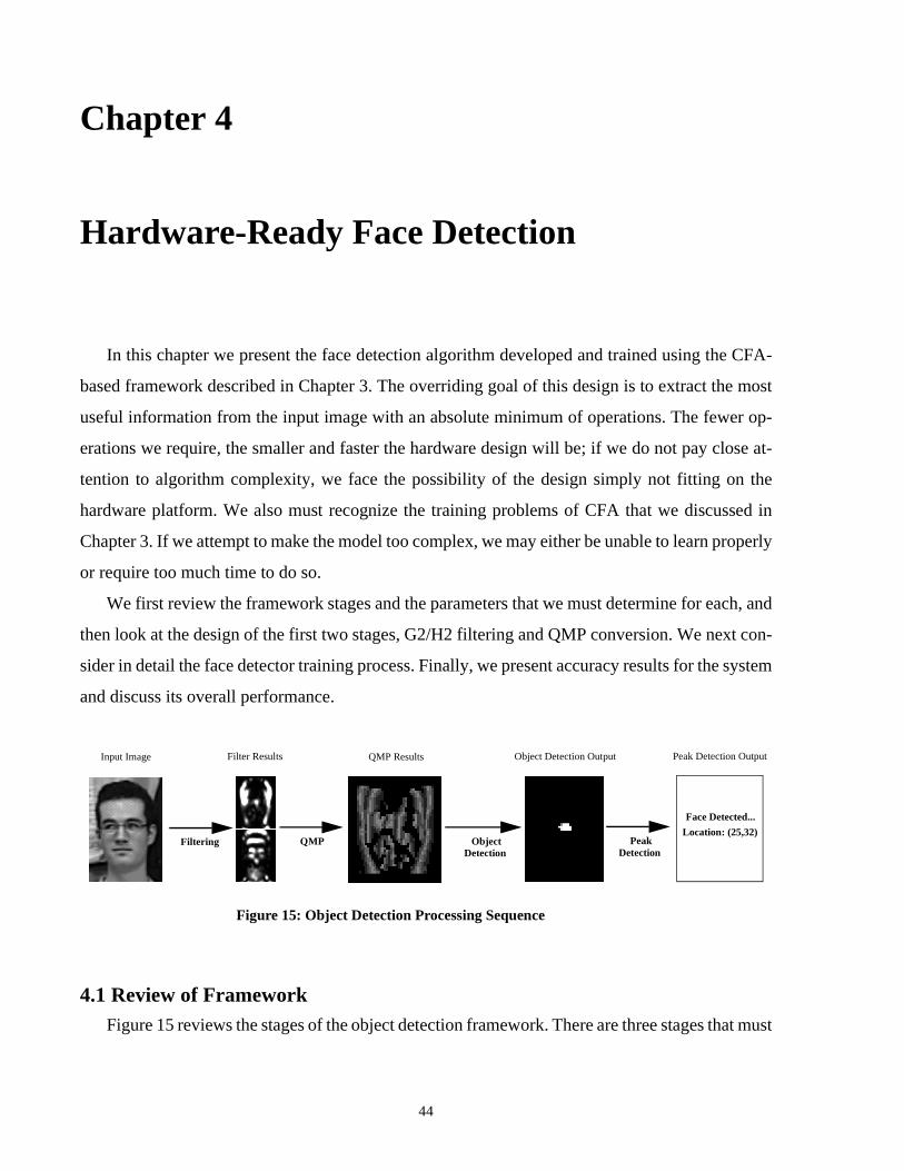
44
Chapter 4
Hardware-Ready Face Detection
In this chapter we present the face detection algorithm developed and trained using the CFA-
based framework described in Chapter 3. The overriding goal of this design is to extract the most
useful information from the input image with an absolute minimum of operations. The fewer op-
erations we require, the smaller and faster the hardware design will be; if we do not pay close at-
tention to algorithm complexity, we face the possibility of the design simply not fitting on the
hardware platform. We also must recognize the training problems of CFA that we discussed in
Chapter 3. If we attempt to make the model too complex, we may either be unable to learn properly
or require too much time to do so.
We first review the framework stages and the parameters that we must determine for each, and
then look at the design of the first two stages, G2/H2 filtering and QMP conversion. We next con-
sider in detail the face detector training process. Finally, we present accuracy results for the system
and discuss its overall performance.
4.1 Review of FrameworkFigure 15 reviews the stages of the object detection framework. There are three stages that must
Figure 15: Object Detection Processing Sequence
Input Image Filter Results QMP Results Object Detection Output
Filtering QMP ObjectDetection
Peak Detection Output
PeakDetection
Face Detected...
Location: (25,32)

Chapter 4: Hardware-Ready Face Detection 45
be customized to the specific application: G2/H2 filtering, QMP conversion, and object detection.
The parameters of the first two stages are relatively simple. For the filtering stage, the parameters
to consider are the orientation and scales (sizes) of filters that will be used. For the QMP conversion
stage, the key parameters are the number of phase bins, the low-magnitude threshold value, and
whether or not to use phase mirroring to ignore filter polarity.
The design of the object detection stage is more complex. We focus below on the composition
of the training set and details of the training algorithm which improve both the speed with which
learning proceeds and the accuracy of the resulting detector.
4.2 Filtering and QMP Conversion ParametersThe goal when choosing filter parameters is to account for as much of the important frequency
spectrum as possible with as few and as small filters as possible. It is difficult, however, to deter-
mine what face information, and thus what frequency range, is important before we train the de-
tector; this is the job of our learning algorithm. Since 9x9 filters are the smallest feasible size for
G2/H2 [16], and the 0 and 90 degree orientations are the simplest to implement and together cover
approximately two-thirds of the orientation spectrum [16], we used these as our initial choice. We
discuss in Section 4.3 how we then adjusted feature scope to find a reasonable spatial frequency
range.
When choosing QMP parameters, we would again like to capture the information we need as
simply as possible. For QMP quantization we use the polarity-invariant phase reflection described
in Chapter 3 and four phase bins centered at 0, 30, 60, and 90 degrees. Phase reflection allows us
to use information from the face/background border, and the four phase bins provide what would
seem to be a reasonable amount of phase resolution. We chose a QMP magnitude threshold of 8,
which is the value at which approximately 60% of the filter results from our training set fell into
the “low magnitude” bin.
4.3 Object Detection Training and TestingIn this section we describe the design and training of the CFA face detector. We first describe
our choice of the number and scope of CFA features used. We then look at the composition of the
training data and several training strategies that we implemented to improve learning speed and de-
tection results.

Chapter 4: Hardware-Ready Face Detection 46
4.3.1 Number and Scope of FeaturesAs we described in Section 3.3, CFA can decompose its input into a set of features using an
iterative algorithm. Results from the same section, however, show that the final number of features
used was very sensitive to learning parameters. We concluded that CFA would not be able to ac-
curately perform this decomposition on complex data in a reasonable amount of time. Given these
results, we chose to limit the CFA face detector to a single feature. Although doing so reduces the
potential accuracy of the detection system, it will also reduce the difficulty of the learning problem
and thus the time required to train the detector.
Given that we are not going to attempt multi-feature decomposition on faces, we can fix the
feature scope before training to be the size of the faces in our training set. As with other parameters,
the choice of face size is driven by two needs: the need to capture important information, and the
need to reduce the complexity of the system. As we change the size of the training set faces, we
change the resolution at which we sample those faces and also shift their spatial frequency content.
Lowering resolution reduces the complexity of the CFA feature but also potentially reduces accu-
racy. Shifting frequency content changes the responses we will get from our 9x9 G2/H2 filter pairs,
and could reduce accuracy if these filters no longer capture important face information. The only
way to find the correct balance between complexity and accuracy is to sample how detection ac-
curacy changes as we vary face size. The metric we used was the number of false positives encoun-
tered for a detection rate of 90%. Table 1 shows the results for four face sizes. We began with the
bounding box of an existing face, 48x45, and then reduced this size by approximately 20% at each
step. The number of false positives remains quite flat until 25x23, at which point it increases sig-
nificantly. We chose the next highest resolution, 30x32, for the implementation. This analysis, per-
formed at the start of this research, did not have the benefit of the full current training set, of full
training parameter optimization, or even of all of our training algorithm modifications. Any future
Face SizeFalse Positives Per Non-Face Image
48x45 12.6
39x37 11.5
32x30 11.9
25x23 13.9
Table 1: Accuracy vs. Face Size

Chapter 4: Hardware-Ready Face Detection 47
implementations should revisit this decision in light of these changes.
4.3.2 Face and Non-Face SetsIn total, we used 770 face images containing approximately 119 different people[30][31]. We
separated ten percent of these for use as a test set, and used the rest to train the face model. We
created three versions of each face image, each randomly scaled within % of the standard mod-
el size of 32 pixels high by 30 pixels wide. We made no effort to similarly introduce random vari-
ation in head tilt. We instead selected the training images to include subjects in natural rather than
arranged poses, such that the variation in head position present in the set would be representative
of that encountered during operation. The images include the left and right borders of the face so
as to take advantage of QMP polarity-invariance. The training and test sets are intentionally diffi-
cult, including noisy images, uncontrolled lighting conditions, and moving subjects.
We also gathered 371 non-face images and similarly split them into training and test
sets[32][33]. The images are densely textured examples of foliage, rocks, fabric patterns, and other
complex materials. These are ideal for testing face detection performance as their complex fractal
structure inevitably generates face-like false positives. We scaled each image to six different sizes
to take advantage of the multi-scale nature of the patterns and increase the number of non-face ex-
amples.
4.3.3 Feature InitializationWhen using any iterative learning strategy there is always the question of how to initialize the
model parameters. Typically they are generated randomly from some reasonable distribution. In
the case of CFA we have a particularly difficult problem. A feature will only learn a pattern if it
already detects some portion of it, however minimally. This is not a problem in theory; given
enough randomly initialized features we will eventually find one that coincidently resembles a pat-
tern in the input. It is, however, a problem in practice since we cannot spend hundreds of training
runs waiting to generate the correct pattern. Instead, we randomly choose one example from the
training set and use it to bias the initialization towards that example’s pattern. To avoid moving the
model to a strong local minimum, the bias is very slight. In practice, this approach eliminated the
need for multiple random restarts.
4.3.4 Fixation and RepetitionIn order to speed the learning process we introduced two strategies. The first of these constrains
10±
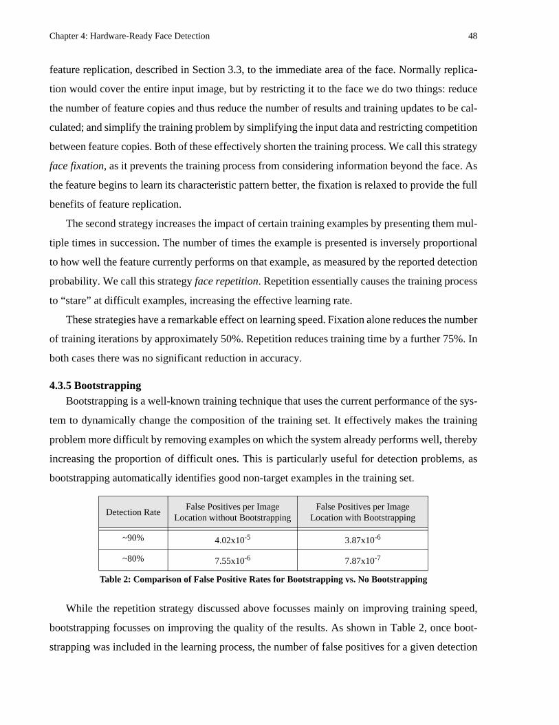
Chapter 4: Hardware-Ready Face Detection 48
feature replication, described in Section 3.3, to the immediate area of the face. Normally replica-
tion would cover the entire input image, but by restricting it to the face we do two things: reduce
the number of feature copies and thus reduce the number of results and training updates to be cal-
culated; and simplify the training problem by simplifying the input data and restricting competition
between feature copies. Both of these effectively shorten the training process. We call this strategy
face fixation, as it prevents the training process from considering information beyond the face. As
the feature begins to learn its characteristic pattern better, the fixation is relaxed to provide the full
benefits of feature replication.
The second strategy increases the impact of certain training examples by presenting them mul-
tiple times in succession. The number of times the example is presented is inversely proportional
to how well the feature currently performs on that example, as measured by the reported detection
probability. We call this strategy face repetition. Repetition essentially causes the training process
to “stare” at difficult examples, increasing the effective learning rate.
These strategies have a remarkable effect on learning speed. Fixation alone reduces the number
of training iterations by approximately 50%. Repetition reduces training time by a further 75%. In
both cases there was no significant reduction in accuracy.
4.3.5 BootstrappingBootstrapping is a well-known training technique that uses the current performance of the sys-
tem to dynamically change the composition of the training set. It effectively makes the training
problem more difficult by removing examples on which the system already performs well, thereby
increasing the proportion of difficult ones. This is particularly useful for detection problems, as
bootstrapping automatically identifies good non-target examples in the training set.
While the repetition strategy discussed above focusses mainly on improving training speed,
bootstrapping focusses on improving the quality of the results. As shown in Table 2, once boot-
strapping was included in the learning process, the number of false positives for a given detection
Detection RateFalse Positives per Image
Location without BootstrappingFalse Positives per Image
Location with Bootstrapping
~90% 4.02x10⁻⁵ 3.87x10⁻⁶
~80% 7.55x10⁻⁶ 7.87x10⁻⁷
Table 2: Comparison of False Positive Rates for Bootstrapping vs. No Bootstrapping

Chapter 4: Hardware-Ready Face Detection 49
rate decreased by almost precisely an order of magnitude.
4.4 Detection Accuracy ResultsTable 3 shows how face detection accuracy varies with respect to both false positives and false
negatives as the face classification threshold is varied. Given the difficulty of the images used to
train and test the system, these results are excellent.
Table 4 shows the accuracy results for other similar face detection methods on their own test
sets (from [12]). Although these should not be directly compared with our results given that differ-
ent test images were used, we can see that on average for a comparable detection rate we have ap-
proximately an order of magnitude more false positives. Since our face classifier is much simpler
than any of those given in Table 4, this may indicate that our test set is not as difficult as those used
by the other methods.
4.5 DiscussionThe most important result we derived from this portion of the research is that we can perform
reasonably accurate face detection using only very simple operations. We are performing minimal
pre-processing and using the equivalent of a single artificial neural network neuron for face clas-
Threshold Detection RateFalse Positives per
Image Location
0.11 90.9% 5.80x10⁻⁶
0.21 90.3% 3.82x10⁻⁶
0.52 87.0% 1.91x10⁻⁶
0.95 80.9% 7.87x10⁻⁷
Table 3: Detection Accuracy vs. Face Classification Threshold
Method Authors Detection RateFalse Positives per
Image Location
Schneiderman et. al. [12] 91.2% 1.66x10⁻⁷
Sung et. al. [13] 84.6% 1.81x10⁻⁷
Rowley et al. [11] 86.6% 9.51x10⁻⁷
Table 4: Examples of Accuracy Performance for Similar Methods (from [12])
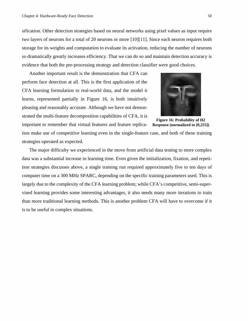
Chapter 4: Hardware-Ready Face Detection 50
sification. Other detection strategies based on neural networks using pixel values as input require
two layers of neurons for a total of 20 neurons or more [10][11]. Since each neuron requires both
storage for its weights and computation to evaluate its activation, reducing the number of neurons
so dramatically greatly increases efficiency. That we can do so and maintain detection accuracy is
evidence that both the pre-processing strategy and detection classifier were good choices.
Another important result is the demonstration that CFA can
perform face detection at all. This is the first application of the
CFA learning formulation to real-world data, and the model it
learns, represented partially in Figure 16, is both intuitively
pleasing and reasonably accurate. Although we have not demon-
strated the multi-feature decomposition capabilities of CFA, it is
important to remember that virtual features and feature replica-
tion make use of competitive learning even in the single-feature case, and both of these training
strategies operated as expected.
The major difficulty we experienced in the move from artificial data testing to more complex
data was a substantial increase in learning time. Even given the initialization, fixation, and repeti-
tion strategies discusses above, a single training run required approximately five to ten days of
computer time on a 300 MHz SPARC, depending on the specific training parameters used. This is
largely due to the complexity of the CFA learning problem; while CFA’s competitive, semi-super-
vised learning provides some interesting advantages, it also needs many more iterations to train
than more traditional learning methods. This is another problem CFA will have to overcome if it
is to be useful in complex situations.
Figure 16: Probability of H2 Response (normalized to [0,255])

51
Chapter 5
Hardware Implementation
In this chapter we present the hardware face detection system. We begin by reviewing our goals
for this implementation and giving an overview of the system as a whole. We then describe each
individual processing unit in detail. At the end of the chapter we provide performance results and
comparisons versus both a serial implementation of the algorithm and serial implementations of
other face detection algorithms.
5.1 GoalsThe goal of this implementation was to achieve full frame-rate face detection using the Trans-
mogrifier 2a and the algorithm described in Chapter 3 and Chapter 4. We also wanted to be able to
detect any number of faces and be able to detect them over the full range of scales from the smallest
detectable face to the largest that fits in the image. Assuming a 320x240 input image and eight scale
steps gives approximately 313644 pixels to process for each frame of video. One frame arrives ev-
ery 33 ms. Given the 12.5 MHz TM-2a clock, the system will need an effective throughput of one
pixel every 1.33 clock cycles to keep up with incoming video. To meet this constraint, the primary
design requirement for the units described below was that each should be able to both consume and
produce one piece of data every cycle, whether that data is a pixel, a filter output, a QMP value, or
a face probability. This ensures that data will “stream” efficiently through the system and allows
each unit to be unproductive for up to one out of every four cycles.
5.2 OverviewFigure 17 shows a block diagram of the system. Image data in the form of pixel greyscale val-
ues flows in from the video input unit, through a scaling unit, and to the X and Y stages of the sep-
arable filter pairs. Filter results are converted into QMP format and passed to the Face Detection
Unit (FDU), which calculates the face detection probabilities. As face probabilities emerge from
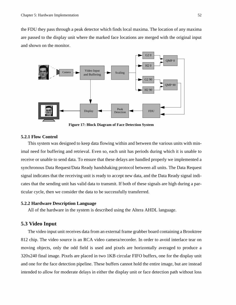
Chapter 5: Hardware Implementation 52
the FDU they pass through a peak detector which finds local maxima. The location of any maxima
are passed to the display unit where the marked face locations are merged with the original input
and shown on the monitor.
5.2.1 Flow ControlThis system was designed to keep data flowing within and between the various units with min-
imal need for buffering and retrieval. Even so, each unit has periods during which it is unable to
receive or unable to send data. To ensure that these delays are handled properly we implemented a
synchronous Data Request/Data Ready handshaking protocol between all units. The Data Request
signal indicates that the receiving unit is ready to accept new data, and the Data Ready signal indi-
cates that the sending unit has valid data to transmit. If both of these signals are high during a par-
ticular cycle, then we consider the data to be successfully transferred.
5.2.2 Hardware Description LanguageAll of the hardware in the system is described using the Altera AHDL language.
5.3 Video InputThe video input unit receives data from an external frame grabber board containing a Brooktree
812 chip. The video source is an RCA video camera/recorder. In order to avoid interlace tear on
moving objects, only the odd field is used and pixels are horizontally averaged to produce a
320x240 final image. Pixels are placed in two 1KB circular FIFO buffers, one for the display unit
and one for the face detection pipeline. These buffers cannot hold the entire image, but are instead
intended to allow for moderate delays in either the display unit or face detection path without loss
Video Inputand Buffering
QMP 0
FDUPeak
DetectionDisplay
Figure 17: Block Diagram of Face Detection System
QMP 90
G2 0
H2 0
G2 90
H2 90
ScalingCamera
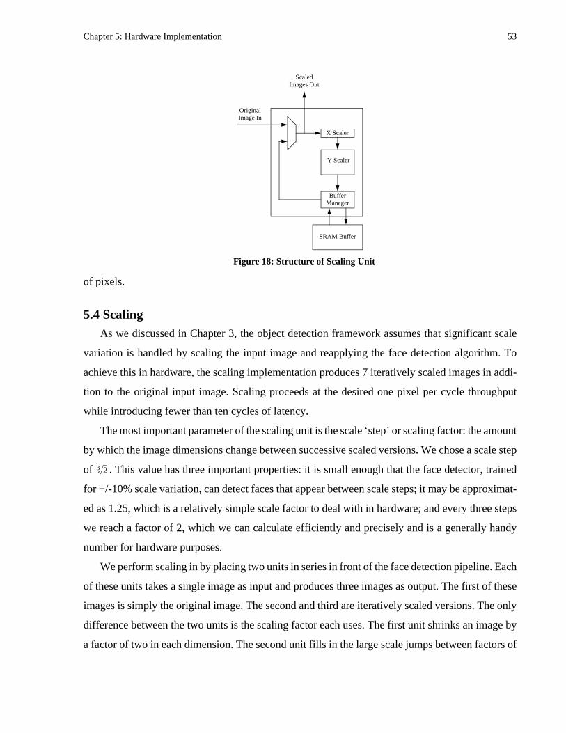
Chapter 5: Hardware Implementation 53
of pixels.
5.4 ScalingAs we discussed in Chapter 3, the object detection framework assumes that significant scale
variation is handled by scaling the input image and reapplying the face detection algorithm. To
achieve this in hardware, the scaling implementation produces 7 iteratively scaled images in addi-
tion to the original input image. Scaling proceeds at the desired one pixel per cycle throughput
while introducing fewer than ten cycles of latency.
The most important parameter of the scaling unit is the scale ‘step’ or scaling factor: the amount
by which the image dimensions change between successive scaled versions. We chose a scale step
of . This value has three important properties: it is small enough that the face detector, trained
for +/-10% scale variation, can detect faces that appear between scale steps; it may be approximat-
ed as 1.25, which is a relatively simple scale factor to deal with in hardware; and every three steps
we reach a factor of 2, which we can calculate efficiently and precisely and is a generally handy
number for hardware purposes.
We perform scaling in by placing two units in series in front of the face detection pipeline. Each
of these units takes a single image as input and produces three images as output. The first of these
images is simply the original image. The second and third are iteratively scaled versions. The only
difference between the two units is the scaling factor each uses. The first unit shrinks an image by
a factor of two in each dimension. The second unit fills in the large scale jumps between factors of
23
Original Image In
Scaled Images Out
X Scaler
Y Scaler
Buffer Manager
SRAM Buffer
Figure 18: Structure of Scaling Unit
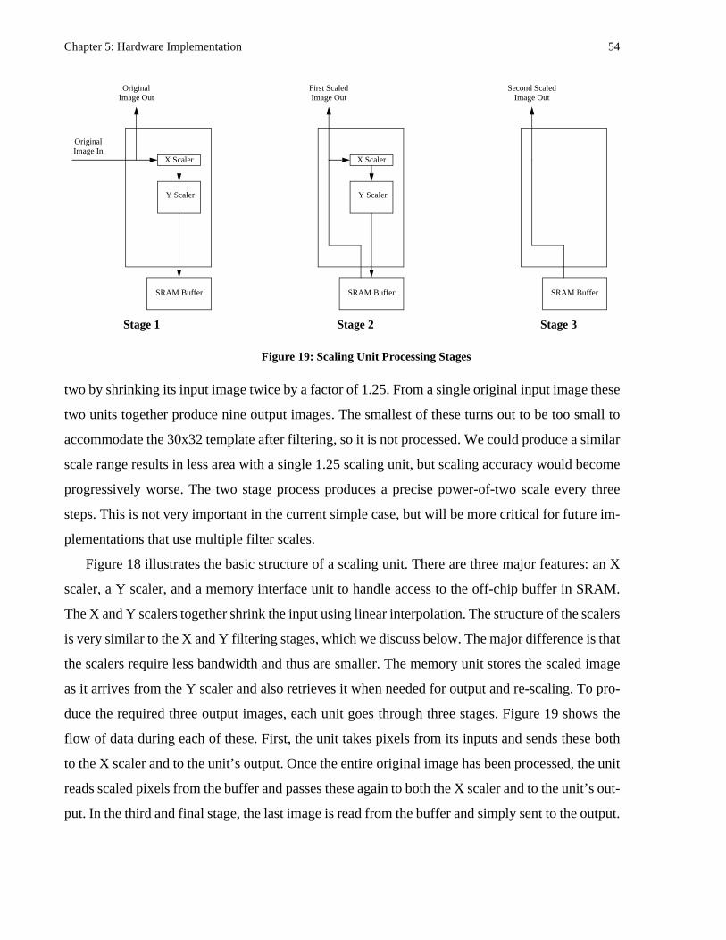
Chapter 5: Hardware Implementation 54
two by shrinking its input image twice by a factor of 1.25. From a single original input image these
two units together produce nine output images. The smallest of these turns out to be too small to
accommodate the 30x32 template after filtering, so it is not processed. We could produce a similar
scale range results in less area with a single 1.25 scaling unit, but scaling accuracy would become
progressively worse. The two stage process produces a precise power-of-two scale every three
steps. This is not very important in the current simple case, but will be more critical for future im-
plementations that use multiple filter scales.
Figure 18 illustrates the basic structure of a scaling unit. There are three major features: an X
scaler, a Y scaler, and a memory interface unit to handle access to the off-chip buffer in SRAM.
The X and Y scalers together shrink the input using linear interpolation. The structure of the scalers
is very similar to the X and Y filtering stages, which we discuss below. The major difference is that
the scalers require less bandwidth and thus are smaller. The memory unit stores the scaled image
as it arrives from the Y scaler and also retrieves it when needed for output and re-scaling. To pro-
duce the required three output images, each unit goes through three stages. Figure 19 shows the
flow of data during each of these. First, the unit takes pixels from its inputs and sends these both
to the X scaler and to the unit’s output. Once the entire original image has been processed, the unit
reads scaled pixels from the buffer and passes these again to both the X scaler and to the unit’s out-
put. In the third and final stage, the last image is read from the buffer and simply sent to the output.
Original Image In
Original Image Out
X Scaler
Y Scaler
SRAM Buffer
Figure 19: Scaling Unit Processing Stages
First Scaled Image Out
X Scaler
Y Scaler
SRAM Buffer
Second Scaled Image Out
SRAM Buffer
Stage 1 Stage 2 Stage 3

Chapter 5: Hardware Implementation 55
5.5 G2/H2 FilteringFrom the scaling unit pixels are passed through separable G2/H2 filters. We have one horizon-
tal and one vertical G2/H2 pair, for a total of four filters. Each filter consists of an X and a Y stage,
with the X stage first to take advantage of the row-oriented data coming from the camera. After
each stage the filter results are reduced to a signed 8-bit representation which allows efficient stor-
age in memory and has been shown in testing to be an adequate level of accuracy.
5.5.1 Design ToolsThe two major design issues common to both X and Y units were the selection of filter coeffi-
cients and the construction of an adder pyramid to sum the multiplied pixels. While the filter coef-
ficients are strictly defined in [16], it may be possible to save hardware area by adjusting the
coefficients values slightly. We may also save area by selecting the order in which to sum the in-
termediate results such that the size of the intermediate adders and registers is minimized. To solve
these problems we developed three software tools.
The first tool generates a set of G2/H2 basis filters of a specified size and optimizes both the X
and Y filter coefficients such that each may be expressed as the sum or difference of two powers
of two, with a slight bias towards exact powers of two. To understand why this is useful, we must
first examine the cost of various mathematical operations in hardware. Table 5 lists the approxi-
mate Altera LCs required for three operations: an 8-bit multiplication, an 8-bit addition, and an 8-
bit fixed shift. We can see that additions are much cheaper than multiplications, and fixed shifts
are free. Multiplication hardware, however, is constructed out of fixed shifts and adders; one shift
and add for every bit of the multiplier term. If one term in the multiplication is constant, the size
of the hardware will shrink roughly in proportion to the number of zeros in the binary representa-
tion of the constant. This is because the shift-and-add hardware for a bit fixed at zero is no longer
needed. If the constant is a power of two, the multiply becomes just a fixed shift and requires no
Operation Logic Cells
8x8-bit Multiplication 121
8-bit Addition 9
8-bit Fixed Shift 0
Table 5: Logic Resources Required for Mathematical Operations
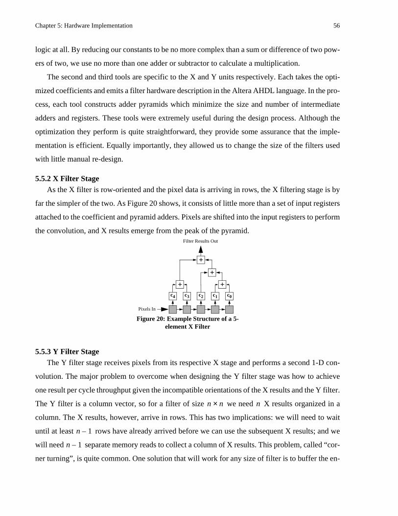
Chapter 5: Hardware Implementation 56
logic at all. By reducing our constants to be no more complex than a sum or difference of two pow-
ers of two, we use no more than one adder or subtractor to calculate a multiplication.
The second and third tools are specific to the X and Y units respectively. Each takes the opti-
mized coefficients and emits a filter hardware description in the Altera AHDL language. In the pro-
cess, each tool constructs adder pyramids which minimize the size and number of intermediate
adders and registers. These tools were extremely useful during the design process. Although the
optimization they perform is quite straightforward, they provide some assurance that the imple-
mentation is efficient. Equally importantly, they allowed us to change the size of the filters used
with little manual re-design.
5.5.2 X Filter StageAs the X filter is row-oriented and the pixel data is arriving in rows, the X filtering stage is by
far the simpler of the two. As Figure 20 shows, it consists of little more than a set of input registers
attached to the coefficient and pyramid adders. Pixels are shifted into the input registers to perform
the convolution, and X results emerge from the peak of the pyramid.
5.5.3 Y Filter StageThe Y filter stage receives pixels from its respective X stage and performs a second 1-D con-
volution. The major problem to overcome when designing the Y filter stage was how to achieve
one result per cycle throughput given the incompatible orientations of the X results and the Y filter.
The Y filter is a column vector, so for a filter of size we need X results organized in a
column. The X results, however, arrive in rows. This has two implications: we will need to wait
until at least rows have already arrived before we can use the subsequent X results; and we
will need separate memory reads to collect a column of X results. This problem, called “cor-
ner turning”, is quite common. One solution that will work for any size of filter is to buffer the en-
+c4 c3 c2 c1 c0
+
+
+
Filter Results Out
Pixels In
Figure 20: Example Structure of a 5-element X Filter
n n× n
n 1–
n 1–
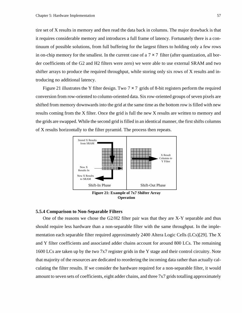
Chapter 5: Hardware Implementation 57
tire set of X results in memory and then read the data back in columns. The major drawback is that
it requires considerable memory and introduces a full frame of latency. Fortunately there is a con-
tinuum of possible solutions, from full buffering for the largest filters to holding only a few rows
in on-chip memory for the smallest. In the current case of a filter (after quantization, all bor-
der coefficients of the G2 and H2 filters were zero) we were able to use external SRAM and two
shifter arrays to produce the required throughput, while storing only six rows of X results and in-
troducing no additional latency.
Figure 21 illustrates the Y filter design. Two grids of 8-bit registers perform the required
conversion from row-oriented to column-oriented data. Six row-oriented groups of seven pixels are
shifted from memory downwards into the grid at the same time as the bottom row is filled with new
results coming from the X filter. Once the grid is full the new X results are written to memory and
the grids are swapped. While the second grid is filled in an identical manner, the first shifts columns
of X results horizontally to the filter pyramid. The process then repeats.
5.5.4 Comparison to Non-Separable FiltersOne of the reasons we chose the G2/H2 filter pair was that they are X-Y separable and thus
should require less hardware than a non-separable filter with the same throughput. In the imple-
mentation each separable filter required approximately 2400 Altera Logic Cells (LCs)[29]. The X
and Y filter coefficients and associated adder chains account for around 800 LCs. The remaining
1600 LCs are taken up by the two 7x7 register grids in the Y stage and their control circuitry. Note
that majority of the resources are dedicated to reordering the incoming data rather than actually cal-
culating the filter results. If we consider the hardware required for a non-separable filter, it would
amount to seven sets of coefficients, eight adder chains, and three 7x7 grids totalling approximately
7 7×
7 7×
Stored X Results from SRAM
New X Results In
New X Results to SRAM
X Result Columns to
Y Filter
Shift-In Phase Shift-Out Phase
Figure 21: Example of 7x7 Shifter Array Operation

Chapter 5: Hardware Implementation 58
5200 LCs in all. The separable implementation therefore reduced resource requirements by just
over 50% versus non-separable filters. The reason this result is not even more dramatic is that al-
though the move to separable filters reduces the coefficient and adder chain hardware by around
75%, it only reduces the data reordering hardware by 33%.
5.6 QMP ConversionThe QMP conversion units each take the filtering results from one of the G2/H2 pairs and con-
vert them into QMP representation. The final result is quantized into 4 phase bins so we only need
to perform two fixed multiplications and three compares, as we describe in Chapter 3. As with the
G2/H2 filters, fixed multiplication coefficients are optimized to be the sum or difference of two
powers of two, and so the multiplier becomes an adder. To complete the QMP conversion we need
to evaluate whether the G2/H2 magnitude is above a fixed threshold. The threshold was set at eight,
so we require only two 3-bit squaring units, one 7-bit adder, and three compare operators.
5.6.1 Efficiency of QMPIn the discussion of the QMP format in Section 3.2 we stated that the format substantially con-
tributed to the efficiency of CFA in hardware. To see why this is true, consider the CFA formula
for the activation given in (EQ 10) below:
(EQ 10)
In this formula is an input value representing the probability that input is currently in
state . In QMP format, the current state is equivalent to the magnitude/phase bin of the response.
Since each G2/H2 result is categorized into one and only one bin, one in (EQ 10) has a proba-
bility of one and the rest have a probability of zero. If we look again at the activation function, we
can see that the computationally expensive sum of products is reduced to a simple selection of one
of the values. In hardware, this selection operation will be much more efficient than mul-
tiplication.
5.7 Face DetectionThe two QMP units pass their results to a Face Detection Unit (FDU), which implements the
akn
akn ins
pkns+
pkns-----------
lns 0=
NS 1–
∑=
ins n
s
ins
pkns+
pkns-----------
ln
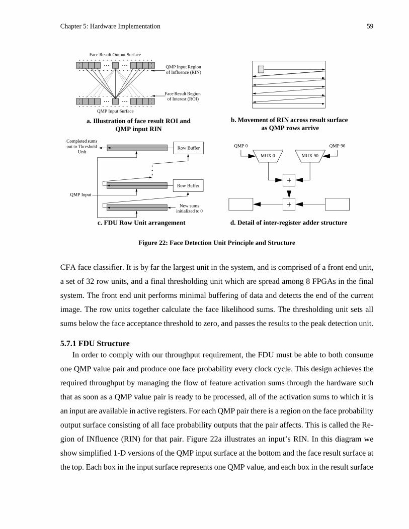
Chapter 5: Hardware Implementation 59
CFA face classifier. It is by far the largest unit in the system, and is comprised of a front end unit,
a set of 32 row units, and a final thresholding unit which are spread among 8 FPGAs in the final
system. The front end unit performs minimal buffering of data and detects the end of the current
image. The row units together calculate the face likelihood sums. The thresholding unit sets all
sums below the face acceptance threshold to zero, and passes the results to the peak detection unit.
5.7.1 FDU StructureIn order to comply with our throughput requirement, the FDU must be able to both consume
one QMP value pair and produce one face probability every clock cycle. This design achieves the
required throughput by managing the flow of feature activation sums through the hardware such
that as soon as a QMP value pair is ready to be processed, all of the activation sums to which it is
an input are available in active registers. For each QMP pair there is a region on the face probability
output surface consisting of all face probability outputs that the pair affects. This is called the Re-
gion of INfluence (RIN) for that pair. Figure 22a illustrates an input’s RIN. In this diagram we
show simplified 1-D versions of the QMP input surface at the bottom and the face result surface at
the top. Each box in the input surface represents one QMP value, and each box in the result surface
... ...
... ...QMP Input Surface
Face Result Output Surface
QMP Input Region of Influence (RIN)
Face Result Region of Interest (ROI)
a. Illustration of face result ROI and QMP input RIN
b. Movement of RIN across result surface as QMP rows arrive
Row Buffer
Row Buffer
...
QMP Input
New sums initialized to 0
Completed sums out to Threshold
Unit
c. FDU Row Unit arrangement
Figure 22: Face Detection Unit Principle and Structure
d. Detail of inter-register adder structure
+
+
MUX 0 MUX 90
QMP 90QMP 0
Chapter 5: Hardware Implementation 60
represents the output of one replicated feature. In solid lines, we show the RIN of the highlighted
QMP value. The shape and size of the RIN is the same as the feature scope.
As the FDU receives its input stream of QMP value pairs, it maintains all of the face activation
sums that will be affected by the next QMP value - that value’s RIN - in a large bank of registers
and updates these sums as QMP values arrive. It is instructive to review how the FDU uses the
QMP inputs to calculate an activation sum an produce a face probability. The value that the FDU
operates on is the activation associated with an output . This requires the calculation, for each
input , of the activation of output with respect to input . These formulas are given below:
(EQ 11)
(EQ 12)
As we discussed in Section 5.6.1, for each input one has a value of 1.0 and the rest are
zero. Each input thus selects of one of the constant values to be added to the overall acti-
vation . As a QMP pair arrives, the FDU must update all of the activations in the input’s RIN by
selecting the appropriate constant for each and adding it to the sum. QMP results arrive at the FDU
from left to right in row orientation. This causes the effective current RIN to scan across the face
from left to right, returning to the left-hand side and dropping down one at the end of each row as
illustrated in Figure 22b. In addition to adjusting the activation values, the FDU must also shift the
current RIN to prepare it for the next input.
The FDU row units implement this add-and-shift operation by storing a row of face results in
on-chip memory and using a bank of 31 registers connected in a chain by 30 adders. Figure 22c
illustrates the arrangement and connection of the row units and shows how results flow through the
FDU. The face results in the current RIN are located in the first 30 registers. When a new QMP
result arrives, its value is used as a selection signal to each of the adders indicating which of several
constant values should be added to each face result. Figure 22d shows this operation in detail. Face
results pass through the adders into the next register, thus performing both RIN shifts to the right,
ak k
n akn k n
ak bkrkn akn
n 0=
NI 1–
∑+=
akn ins
pkns+
pkns-----------
lns 0=
NS 1–
∑=
n inspkns
+
pkns-----------
ln
ak

Chapter 5: Hardware Implementation 61
the right-most edge is filled with new face results pulled out of local memory into the start of the
register bank. As face results arrive at the end of the register bank they are sent upwards to the next
row unit and buffered in local memory for the next left-to-right pass. Results emerging from the
end of the topmost row unit are complete and are passed to the thresholding unit. Results entering
the start of the bottommost row have not been encountered yet and are thus simply zero.
5.7.2 Design ToolsThere is significant complexity involved in properly arranging the model coefficients and de-
termining how may bits are required at each stage of the FDU. To aid in this process we created a
software tool that loads a model file created by the learning algorithm and emits an AHDL descrip-
tion of the FDU circuitry. The tool first quantizes the floating-point model coefficients into a user-
specified number of bits. It then keeps track of the maximum and minimum possible sums at each
stage throughout the row units, allocates as much local memory storage as needed, and sizes the
adders and registers properly. This tool was extremely useful during development as it can quickly
create brand-new circuitry with a different number of coefficient bits or from a model trained using
different learning parameters.
5.7.3 An Alternate DesignAlthough the current FDU structure works well, there is an alternate solution that we initially
overlooked. Figure 22a shows in dashed lines the region on the QMP input surface representing all
of the inputs used by one face probability output. This is the Region of Interest (ROI) of that output.
If a ROI of QMP inputs is buffered and shifted instead of a RIN of face results, the buffered inputs
in the ROI can be used as the input selectors to a large adder pyramid that calculates a single face
result sum. This structure would perform the same task using less memory, fewer adders, and
smaller registers. It would also allow multiple features to share the buffered input values, leading
to a more efficient multi-feature implementation. The current design allows the individual row
units to be more self-contained than this alternative, but on the whole the alternate design would
be preferable for future implementations. Fortunately, the nearly identical shifting structures of the
two solutions will make the new approach easy to implement.
5.8 Peak detectionThe peak detection unit receives thresholded face probabilities from the FDU and detects peaks
in the resulting surface. This is necessary as each face will produce an above-threshold response at

Chapter 5: Hardware Implementation 62
more than one location. Two rows of face results are stored in on-chip memory. As new results
arrive they are shifted along with the buffered results into a 3x3 grid of comparators. If the center
result is greater than or equal to its eight neighbors, the location is counted as a peak and is passed
on to the display unit. In practice this method works well, although a single face will sometimes
generate multiple peaks at adjacent locations or scale steps.
5.9 DisplayThe display unit performs three functions: it buffers the incoming image for display, writes the
face markings given input from the peak detection unit, and merges and displays the last frame’s
image and detection results. There are two pairs of buffers, a draw pair and a display pair, with each
pair containing one image buffer for the input image and one “overlay” buffer for the detection re-
sults. Using two pairs provides double-buffering so that one frame may be displayed while the oth-
er is being drawn. Once a new frame is finished the display and draw buffers are “flipped” during
the monitor’s vertical blank. This avoids the “tearing” of a display image associated with drawing
into a buffer at the same time as it is sent to the monitor.
When the results are being displayed, the display unit uses the value of the overlay pixel to de-
termine what is sent to the monitor: if the overlay pixel is zero, the image pixel value is sent; if it
is one, a green pixel is sent; otherwise the overlay pixel value is sent. This allows the face area to
be marked in a distinct color or even replaced entirely by a pre-set bitmap. Although the image and
overlay buffers are currently stored in the same 2 MB memory bank, they are kept distinct so that
they may be moved into separate banks if more bandwidth is required. This may occur if the input
image resolution is increased in the future.
5.10 Implementation Results
5.10.1 FunctionalityThe system is implemented and running using 9 boards of a 16-board TM-2a system. Detection
is performed over the entire image and at 8 different scales covering a range of nearly 3 octaves.
Any number of faces may be simultaneously detected at any location or scale. Figure 23 shows ac-
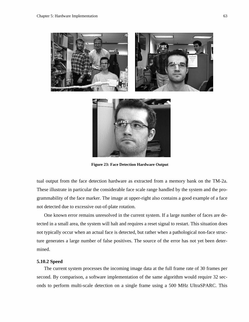
Chapter 5: Hardware Implementation 63
tual output from the face detection hardware as extracted from a memory bank on the TM-2a.
These illustrate in particular the considerable face scale range handled by the system and the pro-
grammability of the face marker. The image at upper-right also contains a good example of a face
not detected due to excessive out-of-plate rotation.
One known error remains unresolved in the current system. If a large number of faces are de-
tected in a small area, the system will halt and requires a reset signal to restart. This situation does
not typically occur when an actual face is detected, but rather when a pathological non-face struc-
ture generates a large number of false positives. The source of the error has not yet been deter-
mined.
5.10.2 SpeedThe current system processes the incoming image data at the full frame rate of 30 frames per
second. By comparison, a software implementation of the same algorithm would require 32 sec-
onds to perform multi-scale detection on a single frame using a 500 MHz UltraSPARC. This
Figure 23: Face Detection Hardware Output
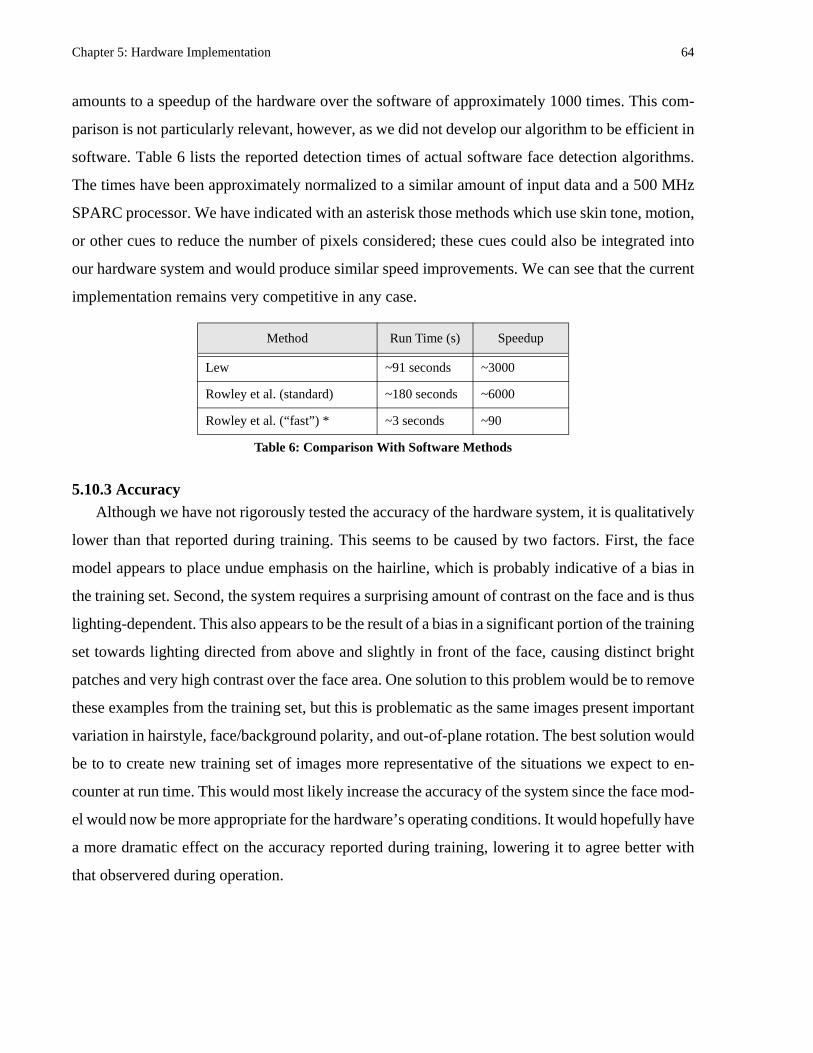
Chapter 5: Hardware Implementation 64
amounts to a speedup of the hardware over the software of approximately 1000 times. This com-
parison is not particularly relevant, however, as we did not develop our algorithm to be efficient in
software. Table 6 lists the reported detection times of actual software face detection algorithms.
The times have been approximately normalized to a similar amount of input data and a 500 MHz
SPARC processor. We have indicated with an asterisk those methods which use skin tone, motion,
or other cues to reduce the number of pixels considered; these cues could also be integrated into
our hardware system and would produce similar speed improvements. We can see that the current
implementation remains very competitive in any case.
5.10.3 AccuracyAlthough we have not rigorously tested the accuracy of the hardware system, it is qualitatively
lower than that reported during training. This seems to be caused by two factors. First, the face
model appears to place undue emphasis on the hairline, which is probably indicative of a bias in
the training set. Second, the system requires a surprising amount of contrast on the face and is thus
lighting-dependent. This also appears to be the result of a bias in a significant portion of the training
set towards lighting directed from above and slightly in front of the face, causing distinct bright
patches and very high contrast over the face area. One solution to this problem would be to remove
these examples from the training set, but this is problematic as the same images present important
variation in hairstyle, face/background polarity, and out-of-plane rotation. The best solution would
be to to create new training set of images more representative of the situations we expect to en-
counter at run time. This would most likely increase the accuracy of the system since the face mod-
el would now be more appropriate for the hardware’s operating conditions. It would hopefully have
a more dramatic effect on the accuracy reported during training, lowering it to agree better with
that observered during operation.
Method Run Time (s) Speedup
Lew ~91 seconds ~3000
Rowley et al. (standard) ~180 seconds ~6000
Rowley et al. (“fast”) * ~3 seconds ~90
Table 6: Comparison With Software Methods
65
Chapter 6
Conclusions and Future Work
6.1 Conclusions and ContributionsThe primary goal of this research was to implement a complex vision task in real-time using a
large configurable hardware system. The vision task we chose was face detection. The research
proceeded in three stages: we designed, implemented, and tested an object detection framework
based on the CFA learning algorithm; we trained a simple face detection system using this frame-
work; and we implemented this system on the Transmogrifier 2a.
We first designed and implemented an object detection framework in software based on the
CFA learning algorithm. The framework is a set of parameterized processing steps that can be eas-
ily adapted to create a detection system for a specific object, and which are geared towards a hard-
ware implementation.
By developing this framework, we made several contributions. The first is the framework as a
whole. Future designers can use it to produce hardware-ready appearance-based detection systems
for essentially any object. The second contribution is the QMP format. From a vision perspective,
QMP preserves important image texture information while providing excellent invariance with re-
spect to lighting changes. From a hardware perspective, it is very compact and cheap to calculate.
The third contribution is the CFA implementation. This is the first application that uses this learn-
ing algorithm. During development and testing we verified some of the anticipated benefits of
CFA, such as multi-feature decomposition and semi-supervised learning, and showed that the al-
gorithm could accurately decompose an artificial data set containing two independent patterns. We
also discovered flaws in the current formulation. The algorithm is unable to learn multiple features
from scratch simultaneously, requiring a iterative work-around that is very prone to becoming
trapped in local minima. The decomposition found using this iterative method is also very sensitive
to regularization. These problems together prevent the algorithm from accurately and efficiently

Chapter 6: Conclusions and Future Work 66
decomposing more complex data. This unfortunately limited the model complexity we could fea-
sibly use for faces to one CFA feature. Nonetheless, the implementation is still very useful and our
experiments provide valuable feedback to CFA development.
We next designed and trained a simple face detection system using the object detection frame-
work. We chose a minimal set of four filters and single CFA feature to perform detection. Once
trained, the system displayed surprisingly good accuracy results given the simplicity of the face
model. We concluded that this was largely due to the QMP representation being an intelligent
choice of input space. The major contribution of this stage was the demonstration that the detection
framework could produce good accuracy on a complex object even when using very simple oper-
ations. Secondary contributions were the training strategies we used to greatly improve both the
speed with which the system trained and the resulting accuracy.
In the last stage of research we implemented the face detection algorithm on the Transmogrifi-
er-2a configurable hardware platform. The system detects any number of faces at any location in
the image over a three-octave scale range, and runs at the full camera frame rate of 30 frames per
second. It requires only nine of the sixteen boards in the TM-2a, leaving nearly half of the system
free for future expansion. Compared to the same algorithm in software running on a 500 MHz
SPARC processor, the hardware system is approximately 1000 times faster. If we make the more
valid comparison to algorithms designed to be efficient in software, we are approximately 3000 to
6000 times faster than systems which restrict themselves to single greyscale images as we do. We
remain approximately 90 times faster than systems which use motion and/or colour information to
reduce the search space. Although we paid for this increased speed with a longer design process,
the time required was only approximately five to ten times over that for a similar software system.
These results validate our assertion that large programmable hardware systems are useful platforms
for the development of real-time vision applications.
The primary contribution of this stage was, of course, the working system. Any future model
improvements gained through CFA development or training modifications can be transferred
quickly to hardware using the FDU circuit generation tool. This tool and the filter generation tools
are also important contribution. These helped greatly during the design process as they allowed us
to quickly incorporate the results of ongoing detection experiments into the hardware design. They
also add to the usefulness of the object detection framework by providing a substantial part of the
path from a detection system created using the framework to a working hardware version.

Chapter 6: Conclusions and Future Work 67
6.2 Future WorkThere are four major directions of future work to explore based on this thesis. The first and sim-
plest direction is to develop new hardware implementations based on the current face detection al-
gorithm. The second direction is to experiment with various parameters of the face detection
algorithm without modifying the basic object detection framework. The third direction is to modify
the framework stages and explore new methods including alternate learning algorithms to CFA.
The fourth direction is to experiment with the CFA formulation itself.
There are promising research opportunities along each of these directions. One option from the
first direction is to add to the hardware system’s functionality. For example, it could be extended
to handle larger input images, or to handle in-plane rotation in the same way as it currently handles
scale. Along the second direction, future work could experiment with using smaller feature scopes
that omit the head/background boundary in concert with QMP conversion that does not use phase
reflection. This would determine whether the boundary of the head provides useful information and
whether phase reflection provides useful lighting invariance. An option from the third direction
would be to use the same G2/H2 filtering and QMP conversion but a better understood learning
method, such as standard neural networks, to experiment with more complex face models. It would
be critical to ensure that the new learning method could gain the same efficiency benefit from using
QMP inputs as does CFA, otherwise the size of the detection hardware could easily increase be-
yond the amount of logic available in the system. Along the fourth direction there is much work to
be done. The most critical task is to improve the stability and learning speed of CFA. Without im-
provement in these areas, it will not be able to perform useful multi-feature decomposition.

68
References
[1] S. McKenna, S. Gong, J. J. Collins. “Face Tracking and Pose Representation,” British Machine
Vision Conference, Edinburgh, Scotland, September 1996.
[2] K. C. Yow, R. Cipolla. “Enhancing Human Face Detection using Motion and Active Con-
tours,” In Proceedings 3rd Asian Conference on Computer Vision, vol. 1, pp 515-522, Hong
Kong, 1998.
[3] K. C. Yow, R. Cipolla. “Scale and Orientation Invariance in Human Face Detection,” In Pro-
ceedings 7th British Machine Vision Conference, vol. 2, pp 745-754, Edinburgh, 1996.
[4] M. S. Lew. “Information Theoretic View-Based and Modular Face Detection,” Proceedings of
the International Conference on Automatic Face and Gesture Recognition, Killington Ver-
mont, October 14-16, 1996, pp. 198-203.
[5] C. Han, H. M. Liao, K. Yu, L. Chen. “Fast Face Detection via Morphology-based Pre-process-
ing,” Technical Report TR-IIS-97-001, Academia Sinica Institute of Information Science,
January 1997.
[6] B. Moghaddam, A. Pentland. “Probabilistic Visual Learning for Object Detection,“ Interna-
tional Conference on Computer Vision, Cambridge, MA, June 1995.
[7] T. Darrell, B. Moghaddam, A. Pentland. “Active Face Tracking and Pose Estimation in an
Interactive Room,” IEEE Conf. on Computer Vision & Pattern Recognition, San Francisco,
CA, June 1996.
[8] P. S. Penev and J. J. Atick. “Local Feature Analysis: A General Statistical Theory for Object
Representation,” Network: Computation in Neural Systems 7(3), pp. 477-500, 1996.
[9] S. McKenna, S. Gong, Y. Raja. ``Segmentation and tracking using colour mixture models,'' in
Asian Conference on Computer Vision, Hong Kong, 8-11 January 1998.

References 69
[10]H. A. Rowley, S. Baluja, and T. Kanade, “Rotation Invariant Neural Network-Based Face
Detection”, Computer Vision and Pattern Recognition, 1998, pages 38-44
[11]H. A. Rowley, S. Baluja, and T. Kanade, “Neural Network-Based Face Detection”, IEEE
Trans. on Patt. Anal. and Mach. Intell., Vol. 20, No. 1, January 1998.
[12]H. Schneiderman, T. Kanade. “Probabilistic Modeling of Local Appearance and Spatial Rela-
tionships for Object Recognition”, IEEE Conference on Computer Vision and Pattern Recog-
nition (CVPR), pp. 45-51. 1998. Santa Barbara, CA
[13]K-K Sung, T. Poggio, “Example-based Learning of View-Based Human Face Detection”,
ACCV 1995 and AI Memo #1521, 1572, MIT.
[14]T. K. Leung, M. C. Burl, P. Perona. “Finding Faces in Cluttered Scenes using Random
Labeled Graph Matching,” Fifth International Conference on Computer Vision, Cambridge,
MA, June 1995.
[15]M.C. Burl, T.K. Leung and P. Perona, “Face Localization via Shape Statistics”, Int. Workshop
Face and Gesture Recognition, 1995, Zurich, Switzerland
[16]W. T. Freeman and E. H. Adelson, “The design and use of steerable filters”, IEEE Trans. on
Patt. Anal. and Mach. Intell., 13(9):891-906, 1991.
[17]E. P. Simoncelli, W. T. Freeman, “The steerable pyramid: A flexible architecture for multi-
scale derivative computation”, In Second International Conference on Image Processing,
Washington, DC, November 1995.
[18]D. Lewis, D. Galloway, M. van Ierssel, J. Rose, P. Chow, “The Transmogrifier-2: A 1 Million
Gate Rapid Prototyping System,” in IEEE Trans. on VLSI, Vol. 6, No. 2, June 1998, pp 188-
198.
[19]D. Lewis, D. Galloway, M. van Ierssel, J. Rose, P. Chow, "The Transmogrifier-2: A 1 Million
Gate Rapid Prototyping System," in FPGA `97, ACM Symp. on FPGAs, Feb 1997, pp. 53-61.
[20]I. Hamer and P. Chow, “DES Cracking on the Transmogrifier 2a,” In Cetin Kaya Koc and
Christof Paar, editors, Workshop on Cryptographic Hardware and Embedded Systems,

References 70
Springer-Verlag Lecture Notes in Computer Science (LNCS 1717), 1999.
[21]A. G. Yee, “Procedural Texture Mapping on FPGAs,” MASc thesis, University of Toronto,
1999.
[22]D. Galloway, “2-D Texture Mapping on TM-2”, Technical Report, University of Toronto,
1996.
[23]S. Brown, J. Rose, "FPGA and CPLD Architectures: A Tutorial," in IEEE Design and Test of
Computers, Vol.12, No. 2, Summer 1996, pp. 42-57.
[24]V. Betz, J. Rose, and A. Marquardt, “Architecture and CAD for Deep-Submicron FPGAs”,
Kluwer Academic Publishers, 1999.
[25]K. Chia, H. J. Kim, S. Lansing, W. H. Mangione-Smith, and J. Villasenor, “High-Performance
Automatic Target Recognition Through Data-Specific VLSI,” in IEEE Transactions on Very
Large Scale Integration Systems Vol. 6, No. 3, Sept. 98, page 364-371.
[26]J. Villasenor, B. Schoner, K. Chia, C. Zapata, H. J. Kim, C. Jones, S. Lansing, and B. Man-
gione-Smith, ”Configurable Computing Solutions for Automatic Target Recognition,” in Pro-
ceedings of the IEEE Symposium on FPGAs for Custom Computing Machines, Apr. 1996,
pp. 70-79.
[27]M. Rencher, B. L. Hutchings, "Automated Target Recognition on SPLASH 2", in Proceedings
of the IEEE Symposium on FPGAs for Custom Computing Machines, April 1997.
[28]R. Petersen, B. L. Hutchings, "An Assessment of the Suitability of FPGA-Based Systems for
Use in Digital Signal Processing", In 5th International Workshop on Field Programmable
Logic and Applications, pp 293-302, August 1995, Oxford, England.
[29]Altera, “Altera 10K FPGA Databook,” 1996.
[30]A.M. Martinez and R. Benavente, “The AR Face Database,” CVC Technical Report #24, June
1998
[31]D.Hond, L. Spacek, “Distinctive Descriptions for Face processing,” Proceeedings of the 8th
British Machine Vision Conference BMVC97, Colchester, England, September 1997, pp.

References 71
320-329.
[32]J.H. van Hateren, A. van der Schaaf, “Independent component filters of natural images com-
pared with simple cells in primary visual cortex,” Proc.R.Soc.Lond, 1998, B 265:359-366.
[33]“MIT Media Lab VisTex Database,” http://www-white.media.mit.edu/vismod/imagery/
VisionTexture/vistex.html.

72
Appendix A
This appendix contains an overview of the CFA formulation.
We begin by stating that the output, , of feature is the probability that the feature is
present given the input data set . We then use Bayes Law to express the output in terms of the
probability of the data given the presence or absence of the feature:
(EQ A1)
(EQ A2)
where is the feature’s activation and is expressed as:
(EQ A3)
If we make the assumption that the individual members, , of the data set are conditionally
independent given the presence or absence of feature , we can express as a function of their
marginal probabilities:
(EQ A4)
ok fk
D
ok p fk D( )=
p D fk( )p fk( )
p D fk( )p fk( ) p D fk( )p fk( )+----------------------------------------------------------------------=
1
1p D fk( )p fk( )p D fk( )p fk( )-------------------------------+
-----------------------------------------=
1
1 eak–
+------------------=
ak
ak lnp D fk( )p fk( )p D fk( )p fk( )-------------------------------
–=
ln=p D fk( )p fk( )
p D fk( )p fk( )-------------------------------
dn
k ak
ak
p fk( )
p fk( )------------
ln lnp dn fk( )
p dn fk( )--------------------
n 0=
ND 1–
∑+=

Appendix A 73
The negative log probabilities of the data members represent error terms between the ex-
pectations of the feature and the actual data, where lower probabilites produce greater error, and
higher probabilities produce lower error. In this case we have two probabilities for each member
of the data set: one set conditioned on the presence of the feature, one conditioned on its absence.
We therefore also have two error terms: one, ,giving the error in the prediction of the data
member if the feature is present, the other, , giving the error if the feature is not present:
(EQ A5)
(EQ A6)
If we consider the component of the activation contributed by , we have:
(EQ A7)
Substituting (EQ A5) and (EQ A6) into (EQ A7), we also have:
(EQ A8)
which shows that we can express the activation as a difference of error terms. If the feature’s
presence would introduce less error than its absence, the activation will be positive. Otherwise, the
activation will be negative.
Each data member is composed of a probability mass function. For each state in the sam-
ple space there is an associated input probability indicating the likelihood that the input is in
that state. The size of the sample space is .
(EQ A9)
The feature has two probability mass function for each input, where the probability of being
in state is if the feature is present and if it is not present. Since the probabilitiy mass
functions must sum to one over the sample space, their values are controlled by a set of lower-level
parameters which ensure this property. They are calculated as follows:
dn{ }
Ekn+
dn Ekn-
Ekn+
p dn fk( )( )ln–=
Ekn-
p dn fk( )( )ln–=
dn
akn lnp dn fk( )
p dn fk( )--------------------
=
akn Ekn-
Ekn+
–( )=
dn s
ins
NS
dn in0 in1 in2 … in NS 1–( ), , ,{ , }=
dn
s pkns+ pkns
-
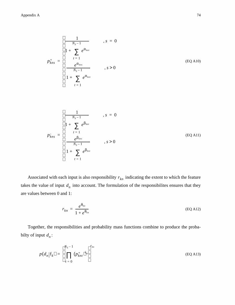
Appendix A 74
(EQ A10)
(EQ A11)
Associated with each input is also responsibility indicating the extent to which the feature
takes the value of input into account. The formulation of the responsibilites ensures that they
are values between 0 and 1:
(EQ A12)
Together, the responsibilities and probability mass functions combine to produce the proba-
bilty of input :
(EQ A13)
pkns+
1
1 eαknt
t 1=
NS 1–
∑+
------------------------------- s, 0=
eαkns
1 eαknt
t 1=
NS 1–
∑+
------------------------------- s, 0>
=
pkns-
1
1 eβknt
t 1=
NS 1–
∑+
------------------------------- s, 0=
eβkns
1 eβknt
t 1=
NS 1–
∑+
------------------------------- s, 0>
=
rkn
dn
rkneθkn
1 eθkn+-----------------=
dn
p dn fk( ) pknt+( )int
t 0=
NS 1–
∏ rkn
=

Appendix A 75
(EQ A14)
(EQ A15)
(EQ A16)
If we substitute the above equations into (EQ A8), we now have:
(EQ A17)
Substituting (EQ A7) into (EQ A4),
(EQ A18)
This completes the derivation of the feature’s activation and output.
Once detection is complete, the ensemble of feature outputs can be considered to be a coding
of the input data set in terms of the feature patterns present in the data. In order to determine how
well our features code the data, we need to measure the error between the data as predicted by the
coding and the original input.
Since more than one feature may be involved, we first need to determine the extent to which
any given feature’s prediction affects the overall prediction for any given data member. This is con-
trolled by a posterior responsibility :
p dn fk( )( )ln rkn pkn0+( ) intαknt
t 1=
NS 1–
∑
+ln
=
p dn fk( ) pknt-( )int
t 0=
NS 1–
∏ rkn
=
p dn fk( )( )ln rkn pkn0-( ) intβknt
t 1=
NS 1–
∑
+ln
=
akn rkn
pkn0+
pkn0-
----------
ln int αknt βknt–( )t 1=
NS 1–
∑
+
=
ak
p fk( )
p fk( )------------
ln rkn
pkn0+
pkn0-
----------
ln
n 0=
ND 1–
∑ rkn int αknt βknt–( )t 1=
NS 1–
∑
n 0=
ND 1–
∑+ +=
rkn

Appendix A 76
(EQ A19)
We also need to calculate the error between a given feature’s prediction and the actual input
given the presence or absence of that feature. This is called the posterior error, and it is expressed
as:
(EQ A20)
We can see that the output of the feature controls the weighting between “present” error and
“not present” error, which is intuitively satisfying.
The total prediction error for the ensemble of features for data member is now simply a sum
of the posterior errors weighted by the posterior responsibilities.
(EQ A21)
The total error for the ensemble over the entire data set is a simple sum of the individual data
member errors:
(EQ A22)
An update rule for any of the model parameters may be found by taking the partial derivative
of the total error with respect to the desired parameter.
rknrknok
rjnoj
j 0=
NF 1–
∑
-----------------------=
Ekn ok Ekn+( ) 1 o– k( ) Ekn
-( )+=
dn
En rknEkn
k 0=
NF 1–
∑=
ED rknEkn
k 0=
NF 1–
∑
n 0=
ND 1–
∑=

vii
List Of Tables
Table 1: Accuracy vs. Face Size ........................................................................................46
Table 2: Comparison of False Positive Rates for Bootstrapping vs. No Bootstrapping ....48
Table 3: Detection Accuracy vs. Face Classification Threshold .......................................49
Table 4: Examples of Accuracy Performance for Similar Methods (from [12]) ...............49
Table 5: Logic Resources Required for Mathematical Operations ....................................55
Table 6: Comparison With Software Methods...................................................................64


![Face Detection & Face Recognition [Teori Informasi 2011]](https://img.pdfslide.us/doc/110x75/548258a6b07959570c8b476a/face-detection-face-recognition-teori-informasi-2011.jpg)