Face Detection and Recognition

Reading: Chapter 18.10

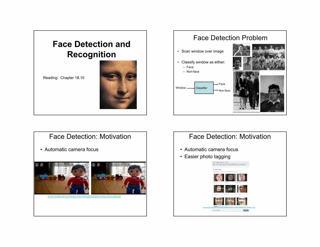
Face Detection Problem

• Scan window over image

• Classify window as either:– Face– Non-face

ClassifierWindowFace

Non-face

Face Detection: Motivation

• Automatic camera focus

http://cdn.conversations.nokia.com.s3.amazonaws.com/wp-content/uploads/2013/09/Nokia-Pro-Camera-auto-focus_half-press.jpghttp://cdn.conversations.nokia.com.s3.amazonaws.com/wp-content/uploads/2013/09/Nokia-Pro-Camera-auto-focus_half-press.jpg

Face Detection: Motivation

• Automatic camera focus• Easier photo tagging

http://sphotos-d.ak.fbcdn.net/hphotos-ak-ash3/163475_10150118904661729_7246884_n.jpg

Face Detection: Motivation

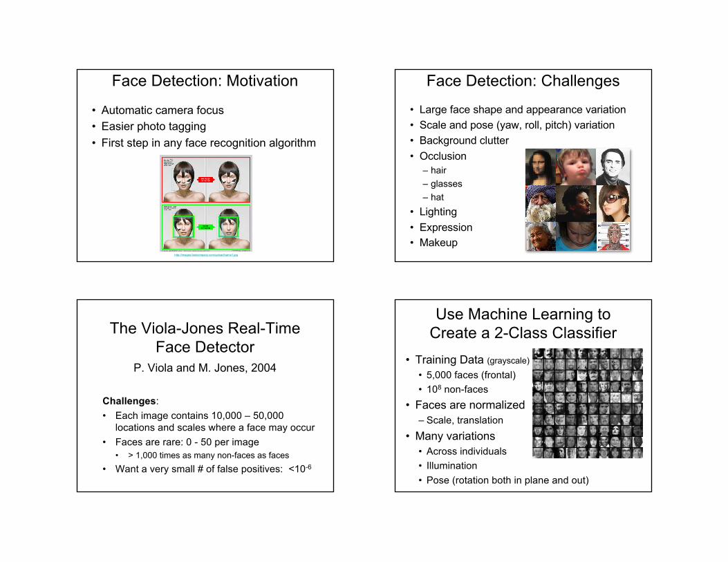
• Automatic camera focus• Easier photo tagging• First step in any face recognition algorithm

http://images.fastcompany.com/upload/camo1.jpg

Face Detection: Challenges

• Large face shape and appearance variation• Scale and pose (yaw, roll, pitch) variation• Background clutter• Occlusion

– hair– glasses– hat

• Lighting• Expression• Makeup

The Viola-Jones Real-Time Face Detector

P. Viola and M. Jones, 2004

Challenges:

• Each image contains 10,000 – 50,000 locations and scales where a face may occur

• Faces are rare: 0 - 50 per image• > 1,000 times as many non-faces as faces

• Want a very small # of false positives: <10-6

• Training Data (grayscale)

• 5,000 faces (frontal)• 108 non-faces

• Faces are normalized– Scale, translation

• Many variations• Across individuals• Illumination

• Pose (rotation both in plane and out)

Use Machine Learning to Create a 2-Class Classifier

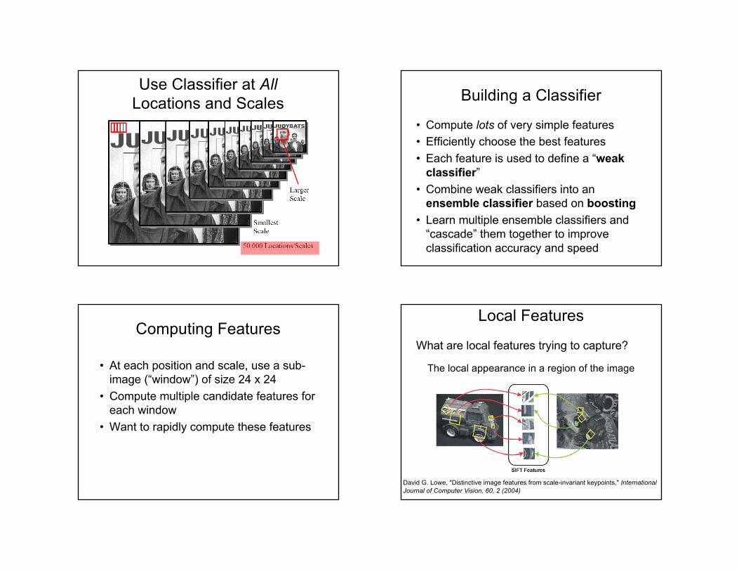
Use Classifier at AllLocations and Scales Building a Classifier

• Compute lots of very simple features• Efficiently choose the best features• Each feature is used to define a “weak

classifier”• Combine weak classifiers into an

ensemble classifier based on boosting• Learn multiple ensemble classifiers and

“cascade” them together to improve classification accuracy and speed

Computing Features

• At each position and scale, use a sub-image (“window”) of size 24 x 24

• Compute multiple candidate features for each window

• Want to rapidly compute these features

Local Features

What are local features trying to capture?

The local appearance in a region of the image

David G. Lowe, "Distinctive image features from scale-invariant keypoints," International Journal of Computer Vision, 60, 2 (2004)

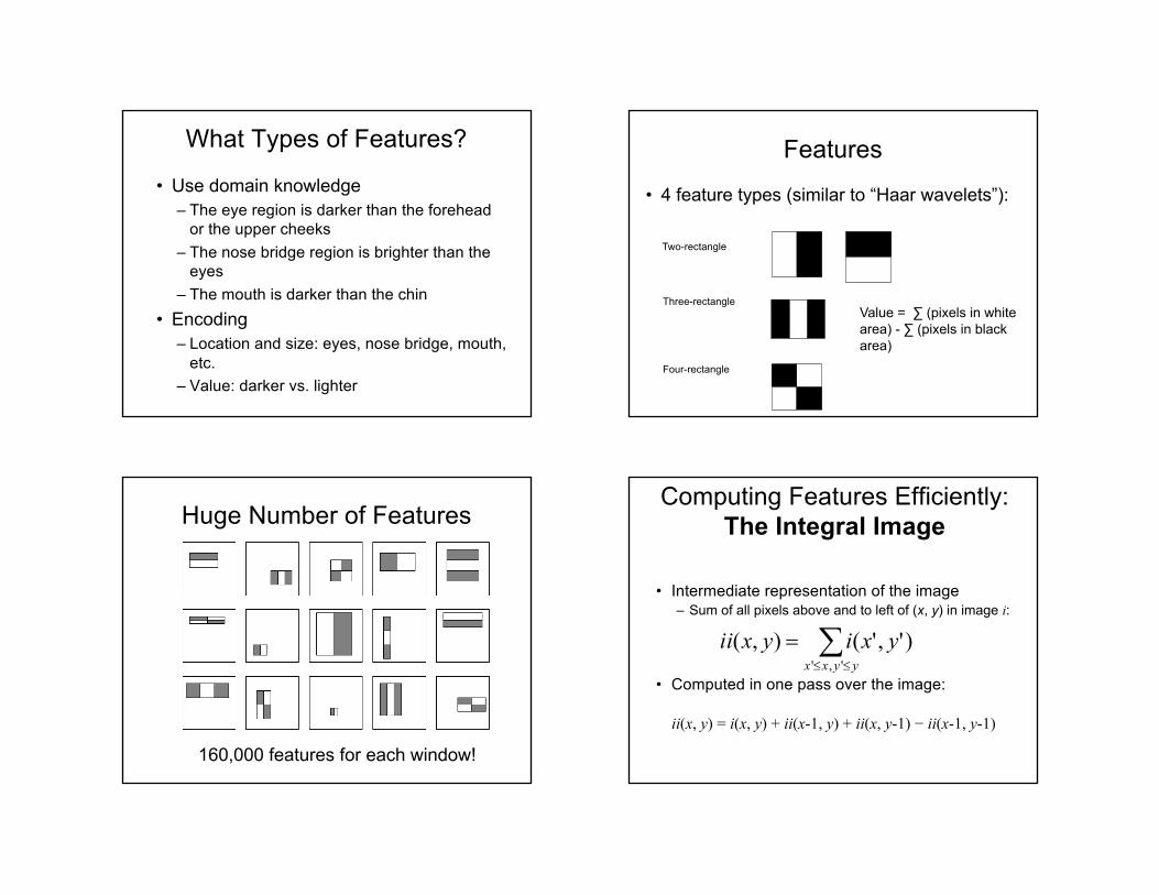
What Types of Features?

• Use domain knowledge– The eye region is darker than the forehead

or the upper cheeks– The nose bridge region is brighter than the

eyes– The mouth is darker than the chin

• Encoding– Location and size: eyes, nose bridge, mouth,

etc.– Value: darker vs. lighter

Features

• 4 feature types (similar to “Haar wavelets”):

Two-rectangle

Three-rectangle

Four-rectangle

Value = ∑ (pixels in white area) - ∑ (pixels in black area)

Huge Number of Features

160,000 features for each window!

Computing Features Efficiently:The Integral Image

• Intermediate representation of the image– Sum of all pixels above and to left of (x, y) in image i:

• Computed in one pass over the image:

ii(x, y) = i(x, y) + ii(x-1, y) + ii(x, y-1) − ii(x-1, y-1)

壣

=yyxx

yxiyxii','

)','(),(

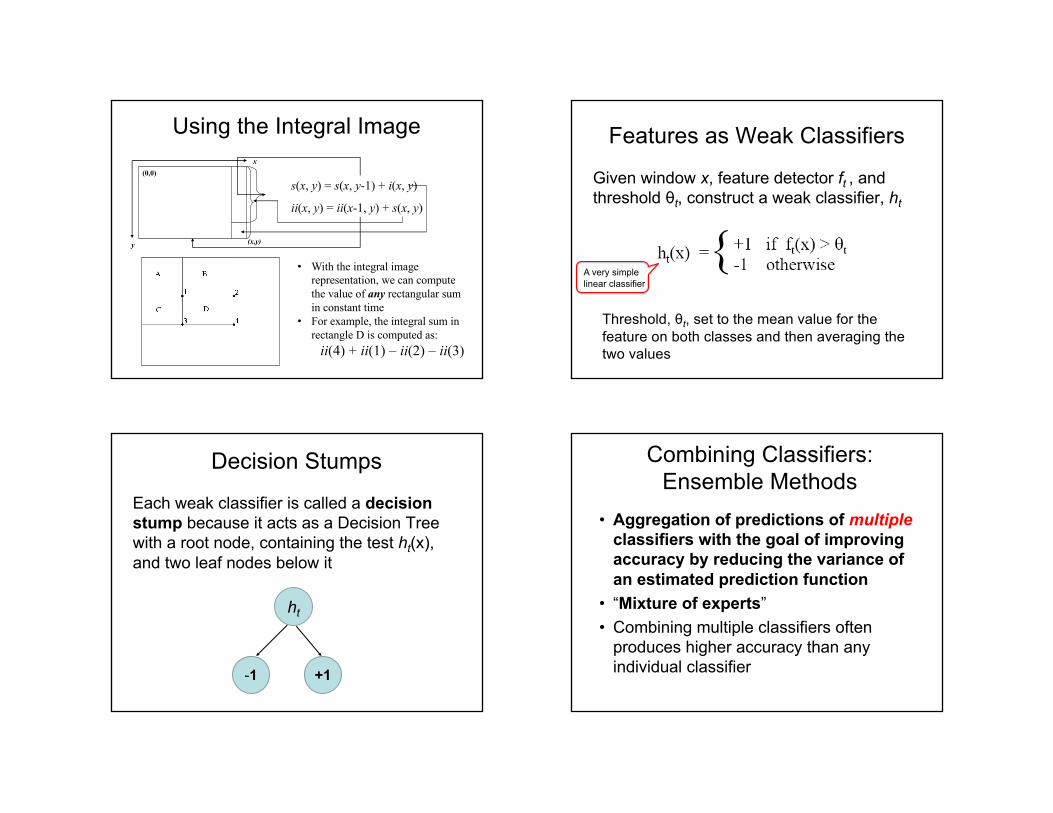
Using the Integral Image

• With the integral image representation, we can compute the value of any rectangular sum in constant time

• For example, the integral sum in rectangle D is computed as:ii(4) + ii(1) – ii(2) – ii(3)

(x,y)

s(x, y) = s(x, y-1) + i(x, y)

ii(x, y) = ii(x-1, y) + s(x, y)

(0,0)x

y

Features as Weak Classifiers

Given window x, feature detector ft , and threshold θt, construct a weak classifier, ht

A very simple linear classifier

Threshold, θt, set to the mean value for the feature on both classes and then averaging the two values

Decision Stumps

Each weak classifier is called a decision stump because it acts as a Decision Tree with a root node, containing the test ht(x), and two leaf nodes below it

ht

-1 +1

• Aggregation of predictions of multipleclassifiers with the goal of improving accuracy by reducing the variance of an estimated prediction function

• “Mixture of experts”• Combining multiple classifiers often

produces higher accuracy than any individual classifier

Combining Classifiers:Ensemble Methods

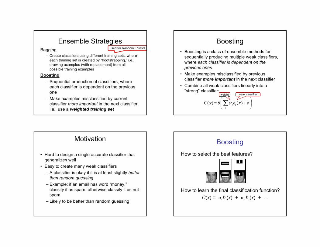
Ensemble StrategiesBagging

– Create classifiers using different training sets, where each training set is created by “bootstrapping,” i.e., drawing examples (with replacement) from all possible training examples

Boosting– Sequential production of classifiers, where

each classifier is dependent on the previous one

– Make examples misclassified by current classifier more important in the next classifier, i.e., use a weighted training set

used for Random Forests

Boosting• Boosting is a class of ensemble methods for

sequentially producing multiple weak classifiers, where each classifier is dependent on the previous ones

• Make examples misclassified by previous classifier more important in the next classifier

• Combine all weak classifiers linearly into a “strong” classifier:

weight weak classifier

Motivation

• Hard to design a single accurate classifier that generalizes well

• Easy to create many weak classifiers – A classifier is okay if it is at least slightly better

than random guessing – Example: if an email has word “money,”

classify it as spam; otherwise classify it as not spam

– Likely to be better than random guessing

BoostingHow to select the best features?

How to learn the final classification function?C(x) = α1 h1(x) + α2 h2(x) + ....

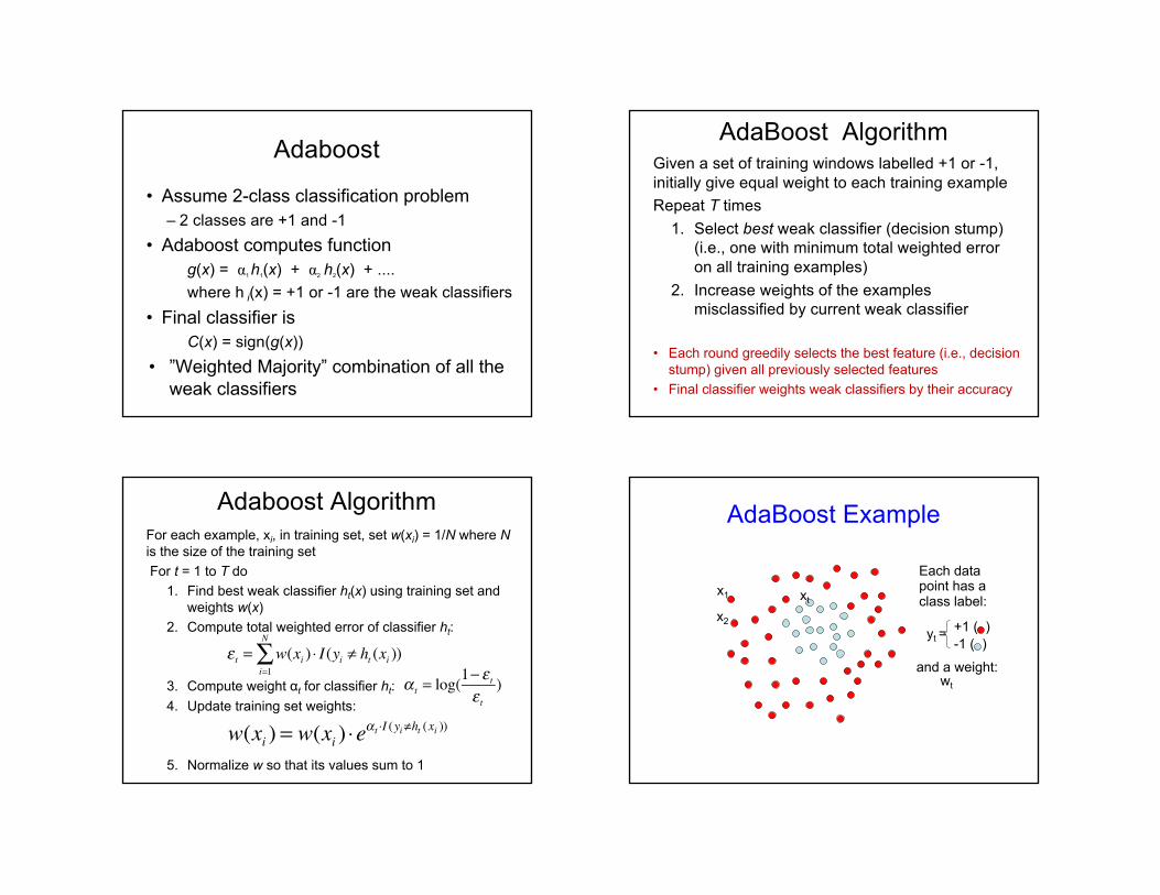
Adaboost

• Assume 2-class classification problem– 2 classes are +1 and -1

• Adaboost computes functiong(x) = α1 h1(x) + α2 h2(x) + ....where h i(x) = +1 or -1 are the weak classifiers

• Final classifier isC(x) = sign(g(x))

• ”Weighted Majority” combination of all the weak classifiers

AdaBoost AlgorithmGiven a set of training windows labelled +1 or -1, initially give equal weight to each training example

Repeat T times

1. Select best weak classifier (decision stump) (i.e., one with minimum total weighted error on all training examples)

2. Increase weights of the examples misclassified by current weak classifier

• Each round greedily selects the best feature (i.e., decision stump) given all previously selected features

• Final classifier weights weak classifiers by their accuracy

Adaboost AlgorithmFor each example, xi, in training set, set w(xi) = 1/N where Nis the size of the training setFor t = 1 to T do

1. Find best weak classifier ht(x) using training set and weights w(x)

2. Compute total weighted error of classifier ht:

3. Compute weight αt for classifier ht: 4. Update training set weights:

5. Normalize w so that its values sum to 1

ε t = w(xi ) ⋅ I(yi ≠ ht (xi ))i=1

N

∑α t = log(

1− ε tε t

)

w(xi ) = w(xi ) ⋅eα t ⋅I (yi≠ht (xi ))

Each data point has a class label:

wt

and a weight:

+1 ( )-1 ( )

yt =

AdaBoost Example

x1

x2

xt

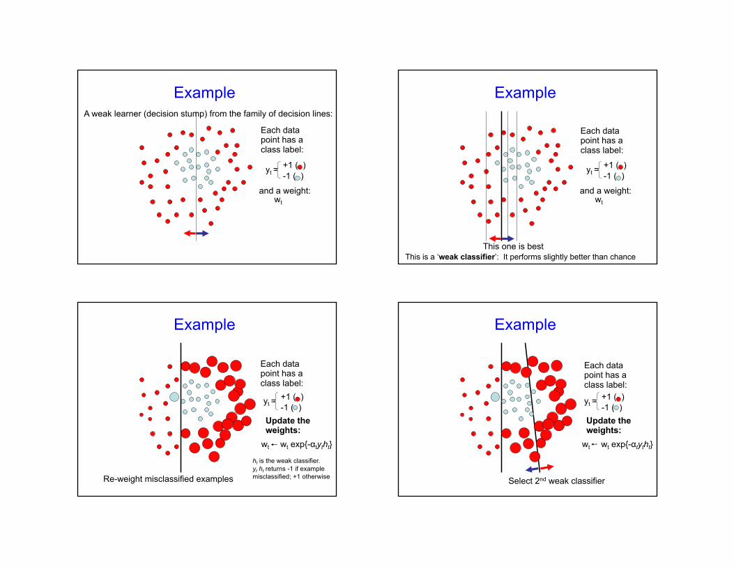
ExampleA weak learner (decision stump) from the family of decision lines:

Each data point has a class label:

wt

and a weight:

+1 ( )-1 ( )

yt =

Example

This one is best

Each data point has a class label:

wt

and a weight:

+1 ( )-1 ( )

yt =

This is a ‘weak classifier’: It performs slightly better than chance

Example

Re-weight misclassified examples

Each data point has a class label:

wt wt exp{-αtytht}

Update the weights:

+1 ( )-1 ( )

yt =

ht is the weak classifier. yt ht returns -1 if example misclassified; +1 otherwise

Example

Select 2nd weak classifier

Each data point has a class label:

wt wt exp{-αtytht}

Update the weights:

+1 ( )-1 ( )

yt =

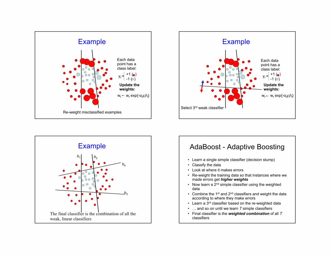
Example

Re-weight misclassified examples

Each data point has a class label:

wt wt exp{-αtytht}

Update the weights:

+1 ( )-1 ( )

yt =

Example

Select 3rd weak classifier

Each data point has a class label:

wt wt exp{-αtytht}

Update the weights:

+1 ( )-1 ( )

yt =

Example

The final classifier is the combination of all the weak, linear classifiers

h1 h2

h3

h4

AdaBoost - Adaptive Boosting• Learn a single simple classifier (decision stump) • Classify the data• Look at where it makes errors• Re-weight the training data so that instances where we

made errors get higher weights• Now learn a 2nd simple classifier using the weighted

data• Combine the 1st and 2nd classifiers and weight the data

according to where they make errors• Learn a 3rd classifier based on the re-weighted data• … and so on until we learn T simple classifiers• Final classifier is the weighted combination of all T

classifiers

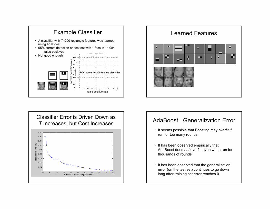
Example Classifier

ROC curve for 200-feature classifier

• A classifier with T=200 rectangle features was learned using AdaBoost

• 95% correct detection on test set with 1 face in 14,084false positives

• Not good enough

false positive rate

corre

ct d

etec

tion

rate

Learned Features

Classifier Error is Driven Down as T Increases, but Cost Increases AdaBoost: Generalization Error

• It seems possible that Boosting may overfit if run for too many rounds

• It has been observed empirically that AdaBoost does not overfit, even when run for thousands of rounds

• It has been observed that the generalization error (on the test set) continues to go down long after training set error reaches 0

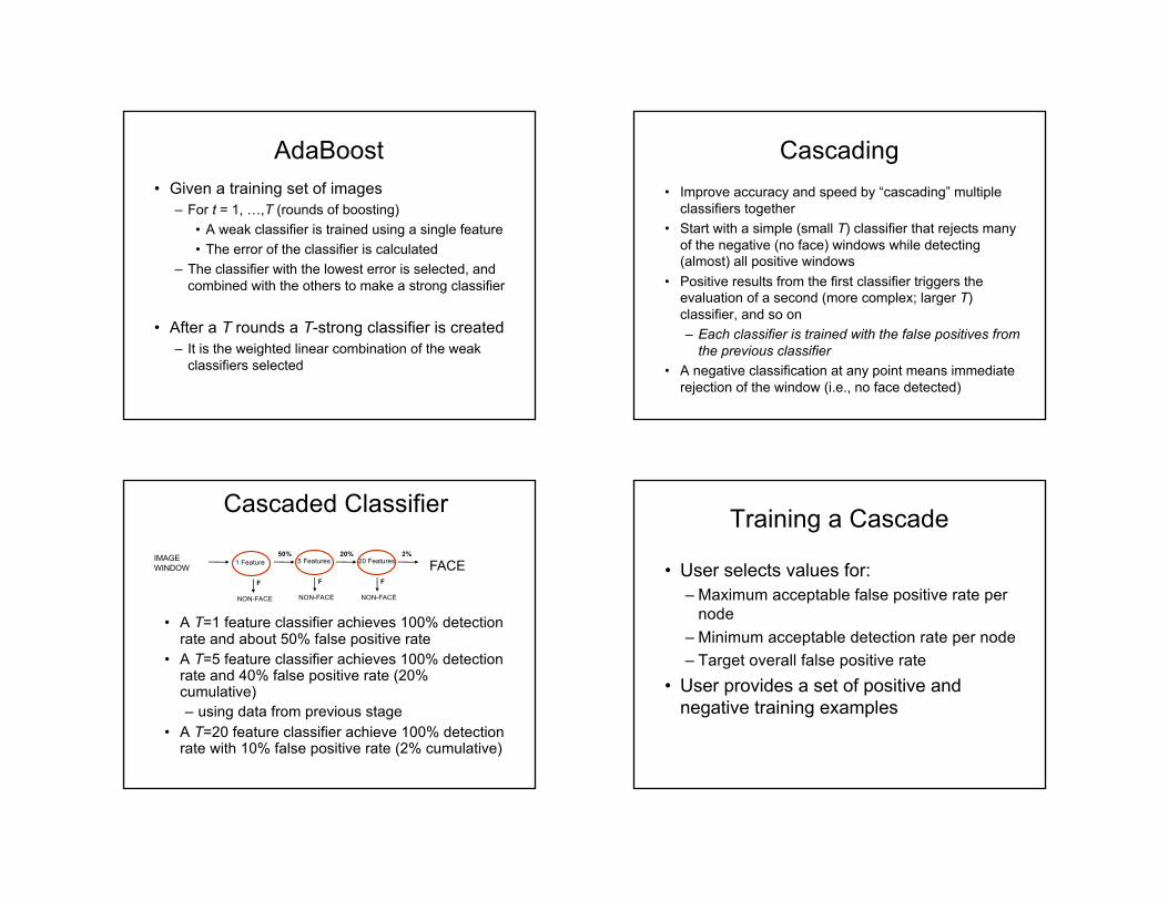
AdaBoost• Given a training set of images

– For t = 1, …,T (rounds of boosting)• A weak classifier is trained using a single feature• The error of the classifier is calculated

– The classifier with the lowest error is selected, and combined with the others to make a strong classifier

• After a T rounds a T-strong classifier is created– It is the weighted linear combination of the weak

classifiers selected

Cascading• Improve accuracy and speed by “cascading” multiple

classifiers together• Start with a simple (small T) classifier that rejects many

of the negative (no face) windows while detecting (almost) all positive windows

• Positive results from the first classifier triggers the evaluation of a second (more complex; larger T) classifier, and so on– Each classifier is trained with the false positives from

the previous classifier• A negative classification at any point means immediate

rejection of the window (i.e., no face detected)

Cascaded Classifier

5 Features50%

F

NON-FACE

20 Features20% 2%

FACEF

NON-FACE

IMAGEWINDOW

1 Feature

F

NON-FACE

• A T=1 feature classifier achieves 100% detection rate and about 50% false positive rate

• A T=5 feature classifier achieves 100% detection rate and 40% false positive rate (20% cumulative)– using data from previous stage

• A T=20 feature classifier achieve 100% detection rate with 10% false positive rate (2% cumulative)

Training a Cascade

• User selects values for: – Maximum acceptable false positive rate per

node– Minimum acceptable detection rate per node– Target overall false positive rate

• User provides a set of positive and negative training examples

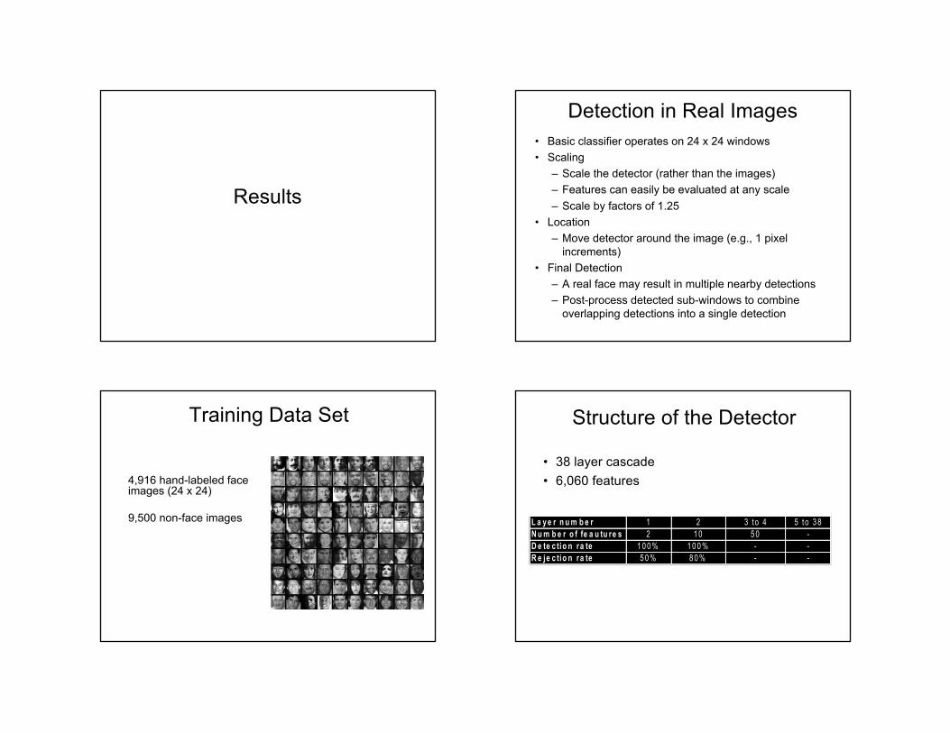
Results

Detection in Real Images• Basic classifier operates on 24 x 24 windows• Scaling

– Scale the detector (rather than the images)– Features can easily be evaluated at any scale– Scale by factors of 1.25

• Location– Move detector around the image (e.g., 1 pixel

increments)• Final Detection

– A real face may result in multiple nearby detections – Post-process detected sub-windows to combine

overlapping detections into a single detection

Training Data Set

4,916 hand-labeled face images (24 x 24)

9,500 non-face images

Structure of the Detector

• 38 layer cascade• 6,060 features

L a y e r n u m b e r 1 2 3 to 4 5 to 3 8N u m b e r o f fe a u tu re s 2 1 0 5 0 -D e te c tio n ra te 1 0 0 % 1 0 0 % - -R e je c tio n ra te 5 0 % 8 0 % - -

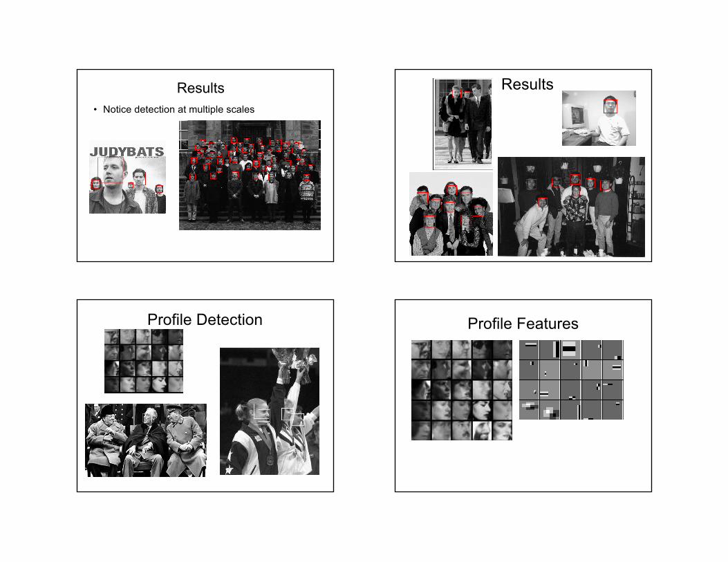
Results• Notice detection at multiple scales

Results

Profile Detection Profile Features

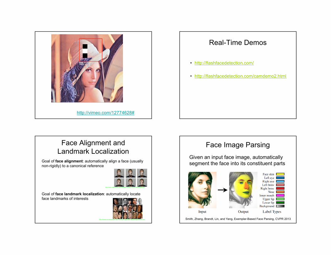
http://vimeo.com/12774628#

Real-Time Demos

• http://flashfacedetection.com/

• http://flashfacedetection.com/camdemo2.html

Face Alignment and Landmark Localization

Goal of face alignment: automatically align a face (usually non-rigidly) to a canonical reference

Goal of face landmark localization: automatically locate face landmarks of interests

http://www.mathworks.com/matlabcentral/fx_files/32704/4/icaam.jpg

http://homes.cs.washington.edu/~neeraj/projects/face-parts/images/teaser.png

Face Image ParsingGiven an input face image, automatically segment the face into its constituent parts

Smith, Zhang, Brandt, Lin, and Yang, Exemplar-Based Face Parsing, CVPR 2013

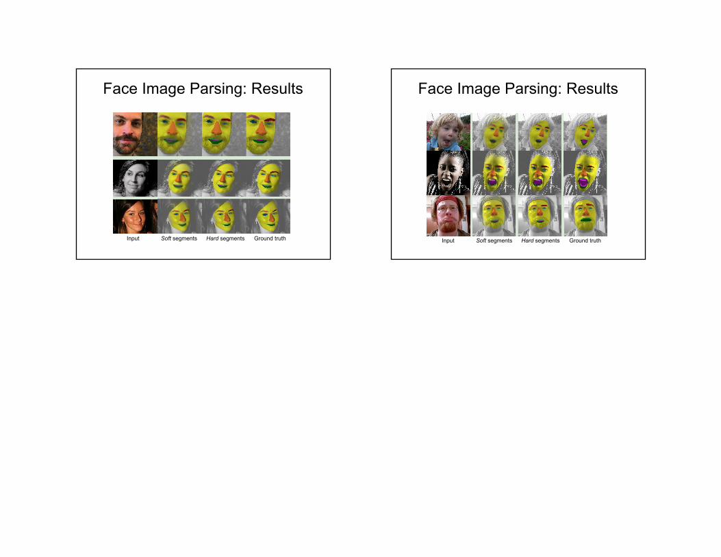
Face Image Parsing: Results

+Input Soft segments Hard segments Ground truth

Face Image Parsing: Results

+Input Soft segments Hard segments Ground truth