1 INTRODUCTION

Many practical engineering systems change dynamic parameters during their operation. Possible reason of parameters change can be damage, changes of operational conditions or occur some physical phenomena causing changes in dynamics of the system. Analysis of nonstationary sys-tems are more difficult than in stationary case and require a dedicated method of identification. Nonstationary linear mechanical systems are those systems whose parameters as stiffness, natu-ral frequency, mass and damping ratios or statistical properties of an input signal (such as mean value and variance) are time dependent. Changes of this parameters can be caused by many fac-tors, from changes of environmental conditions like temperature, humidity, changes of structure geometry, variable operational conditions to damage. In practice, many engineering structures like traffic – excited bridges, rotating machinery working with varying speed, aircrafts, robots, cranes and many others should be treated as non – stationary systems. Analysis of non – statio-nary systems require application of dedicated method which can not be based on averaging which is most popular way of improving quality of parameters identification results. In some cases, when changes of parameters are slow, the system can be treated as stationary in given time interval. Firsts attempts of non – stationary systems parameters identification consists in adaptation of classical identification method of Linear Time Invariant (LTI) systems. Main problem of this approach was to adapt classical algorithm to operate on small number of sam-ples, where quasistationarity condition was assumed. Within the space of the last several dozen years many method for non – stationary system identification were created. The method based on different algorithms like for example BTLS (Bootstarpped Total Least Squares) , RLS (Re-

Real time estimation of modal parameters of non-stationary systems using adaptive wavelet filtering and Recursive Least Square algorithm.

Andrzej Klepka AGH University of Science and Technology, Krakow, Poland

Tadeusz Uhl AGH University of Science and Technology, Krakow, Poland

ABSTRACT: The paper presents a method of modal parameter estimation based on RLS (Re-cursive Least Square) algorithm, and wavelet filtering. The wavelet filtering gives possibility to decoupling frequency components of signal response of structure. This operation can also re-duce the order of the signal model estimated by RLS algorithm. An additional advantage of this method is the possibility of adapting the wavelet filter parameters to the changing parameters of the system. Reduced model order significantly reduces the time of estimation of modal parame-ters, which enables the real – time implementation of the method. Due to recursively updated covariance matrix of model parameters, the confidence intervals of modal parameters can be al-so estimated. All routines have been implemented and tested in MATLAB®. The hardware rea-lization of the algorithm have been achieved employing FPGA (Field Programmable Gate Ar-ray) technology. The method have been tested on simulated data delivered by an AIRBUS team and on the test bed with a variable stiffness.

2 IOMAC'11 – 4th International Operational Modal Analysis Conference

dt

a

btgtx

abaxWg

*1,

cursive Least Square), TARMA (Time-dependent Autoregressive Moving Average), Recursive Subspace and many others. In the literature many of application of this method can be found.

One of an example of phenomenon causing nonstationary behavior of aircrafts (but not only) can be flutter phenomenon. Unstable vibrations of an airplane can be a reason of a catastrophic failure of the aircraft (Kehoe 1995). A critical instability phenomenon is known as “aero-elastic flutter”. In the literature (Brenner M.J. 1997, Reed 1981, Cooper 2006) many cases of flutter phenomena are carefully studied. The importance of accurate definition aeroelastic effects such as flutter on flight vehicles are evident and in fact can be traced earliest days of manned aviation itself. For preventing from a flutter phenomenon, the airplane is submitted to a flight flutter test-ing procedure, with incrementally increasing altitude and airspeed. Flight flutter testing proce-dure can be formulated as procedure of stability test. One possible solution is to find instable poles (which are responsible of flutter phenomena) of the aircraft structure with employing modal model parameters. Important challenges of the in-flight modal analyses are the limited choices for measured excitation inputs, and the presence of unmeasured natural excitation input (e.g. turbulence). A better exploitation of flight test data can be achieved by using output-only system identification methods, which exploits recorded vibration data under natural excitation conditions, without artificial control surface excitation and other types of excitation inputs (Kehoe 1995, Reed 1981). There are many different modal parameters identification methods that could be used for flight flutter testing (Brenner 2003, Cooper 2006, Brenner M.J. 1997, Klepka A. Uhl T 2008, Verboven P. 2004).

This paper presents a recursive modal parameters identification method of nonstationary sys-tems. The classical RLS algorithm is supported wavelet transform which allows decouple com-ponents of the signal response and reduce the order of the model. This operation greatly accele-rated the process of modal parameter estimation, which is a critical part of the algorithm. Such an approach allow real – time implementation of the algorithm. The method was applied to identification of modal parameters of airplane model and to track frequency changes of the system with variable stiffness.

2 RECURSIVE METHOD OF MODAL PARAMETERS ESTIMATION

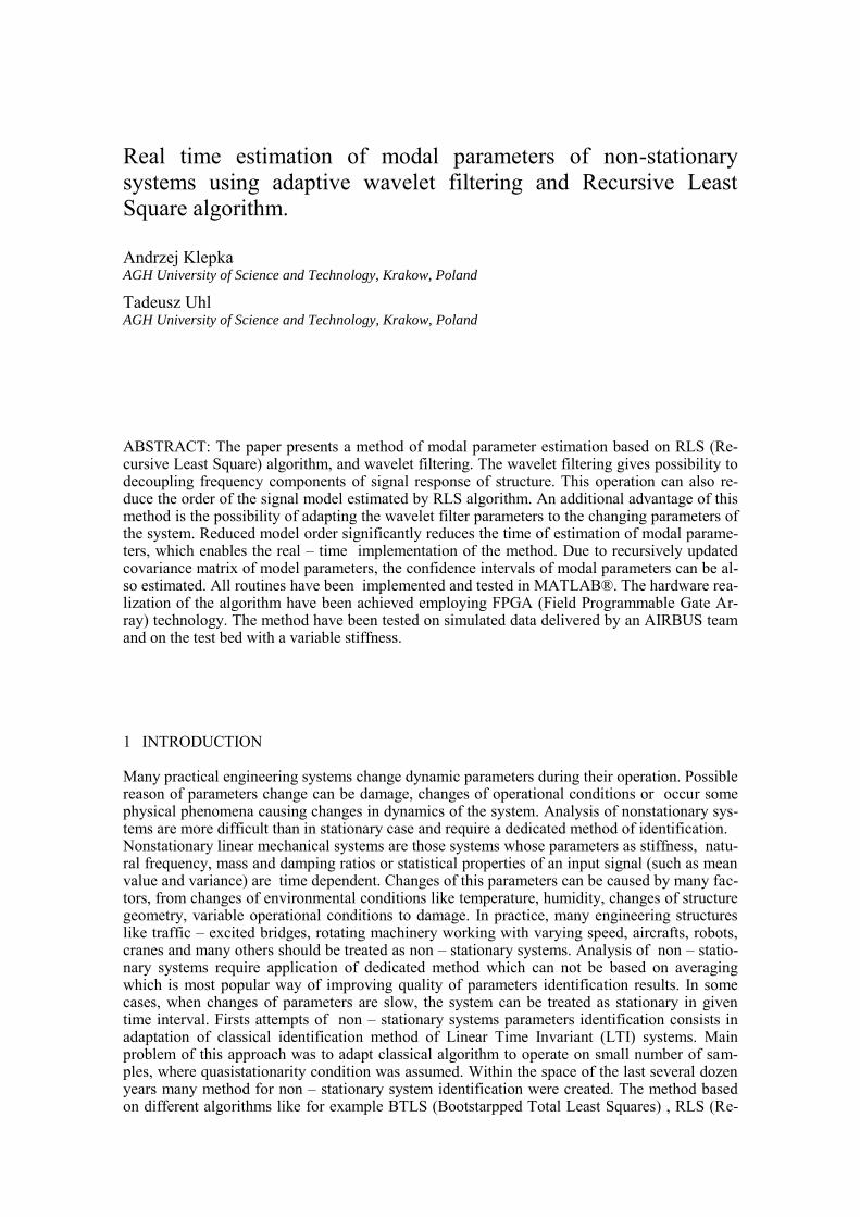
The proposed algorithm consists of three main parts. In the first step the signal is decom-posed by wavelet transform. In second step model parameters are estimated. In third step a modal parameters and their standard deviation are determined. Organization of the algorithm shown in Figure 1.

Figure 1 : Organization of the algorithm. All parts of the algorithm are described in detail in the next subsections.

2.1 Wavelet Transform

The wavelet analysis is a method of signal decomposition. As a result of the wavelet analy-

sis, in contradiction to the Fourier transform, elementary signals – so called wavelets – are ob-tained. Wavelet functions are continuous, oscillated with various duration times and spectrums. From the mathematical point of view, a continuous wavelet transform (CWT) of a signal x(t)

can be defined as (Uhl .T 2005) (K. A. Uhl T. 2006):

(1)

3

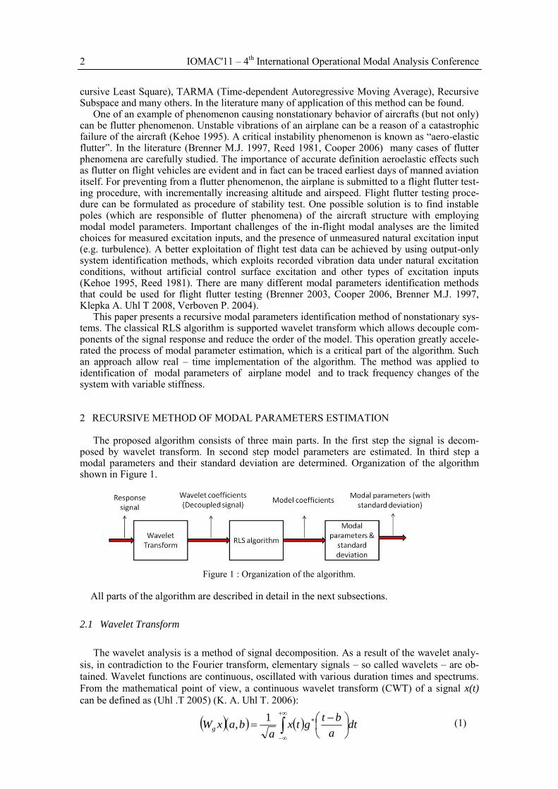
Using properties of wavelet transform, can be proved mathematically that this kind of time frequency analysis decoupling frequency components of signal. Utilizing above – mentioned feature as signal processing method each component of the signal can be analyzed separately. Additionally order of the model using to identification process is reduced to model for only giv-en frequency component of the signal. This approach decrease computational effort which can be significant for higher model order systems especially during finding a roots of the characte-ristic polynomial. Besides, it is not always demand to track all natural frequencies and damping ratios of the system. Using wavelet filtration only critical modes (from the point of view of process) can be track. It also reduces demand for computational capability which increase appli-cability of method and makes real – time implementation process easier. Schematically process of frequency component decoupling is shown in Figure 2. More detailed information about fre-quency components decoupling can be found at (Uhl .T 2005).

Figure 2 : Wavelet based signal components decoupling.

2.2 Recursive Least Square algorithm

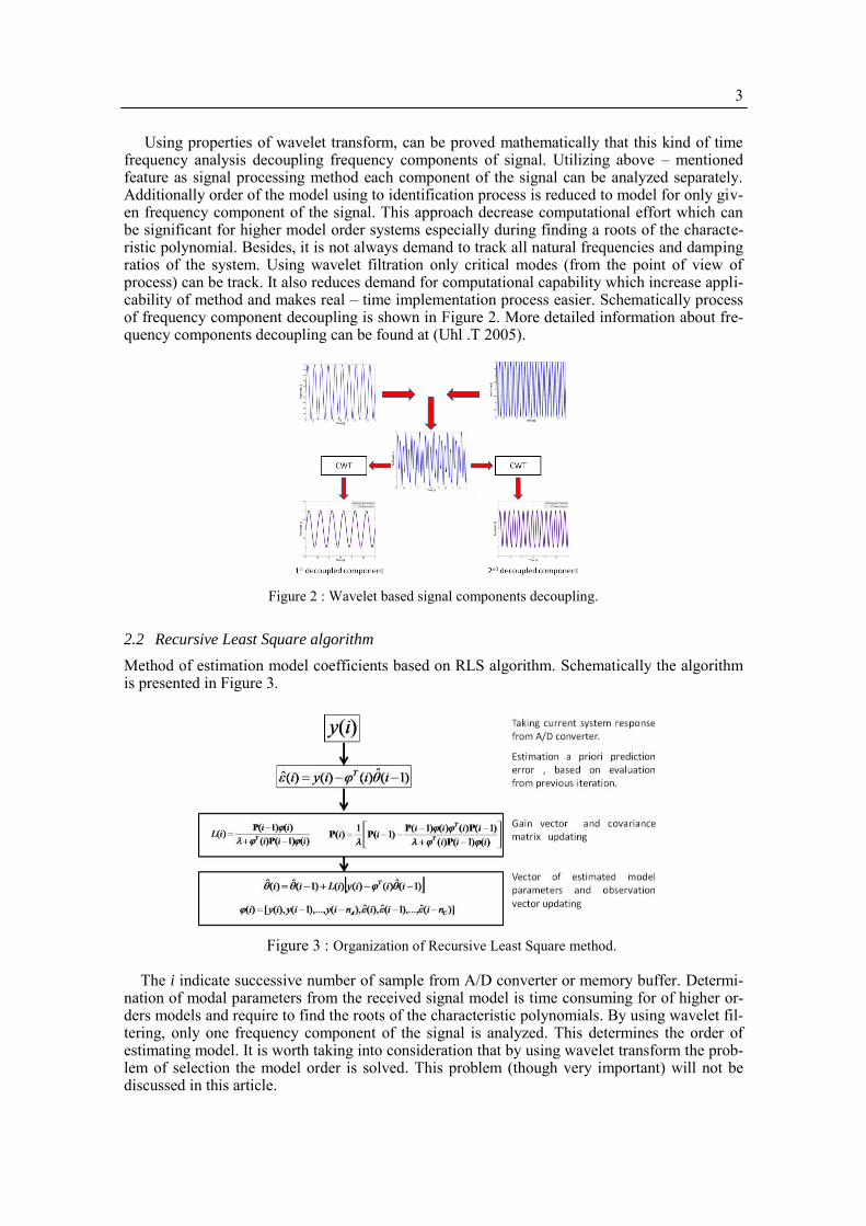
Method of estimation model coefficients based on RLS algorithm. Schematically the algorithm is presented in Figure 3.

Figure 3 : Organization of Recursive Least Square method.

The i indicate successive number of sample from A/D converter or memory buffer. Determi-nation of modal parameters from the received signal model is time consuming for of higher or-ders models and require to find the roots of the characteristic polynomials. By using wavelet fil-tering, only one frequency component of the signal is analyzed. This determines the order of estimating model. It is worth taking into consideration that by using wavelet transform the prob-lem of selection the model order is solved. This problem (though very important) will not be discussed in this article.

4 IOMAC'11 – 4th International Operational Modal Analysis Conference

ss T

aaa

T

aaa

211211 42

1arctan4

2

1ln

2

1

2

2

12

2

1

2

2

2

2

1

2

1

2

2

1

2

1

2

1,4

2

1arctan4

2

1ln

42

1ln

ss

sT

aaa

T

aaa

T

aaa

T

NNn EP ˆˆˆˆ

00

TNnN

T

N

T

NNNn JPJJEJP ˆˆˆˆˆˆˆˆˆ

00

n

mmm

n

n

fff

fff

fff

J

21

2

2

2

1

2

1

2

1

1

1

2.3 Modal parameters and their standard deviation

Thanks to low (equal to 2) model order, estimation of modal parameters is reduced to the ap-plication of simple mathematical formulas. For example, the natural frequency of the system and the corresponding damping coefficient can be determined from the dependence:

(2) where: a1, a2 – model coefficients, - natural frequency, - damping ratio,

Ts – sampling time. When analytical dependences between modal and model parameters are known it is possible

to calculate covariance matrix of modal parameters (Andersen P. 2007, Andersen 1997).

(3)

where: E - is the expected value, ],,...,,[ˆ2211 nsN - is a vector of estimated

modal parameters, 0 - is a vector of true modal parameters, nP ˆˆ - is a covariance matrix of

modal parameters. Using Taylor series expansion method, the covariance matrix of modal pa-rameters can be expressed as:

(4)

Where NJ ̂ is the following Jacobi matrix:

(5)

and - is the vector of model parameters. In general case the Jacobi matrix is impossible to de-termine, that is why in the considered case the numerical differentiation with the Central Differ-ence method was applied. When the standard deviation of modal parameters is known, the con-fidence bounds can be easy determined using “n sigma” method. In this work “three sigma” was assumed. It means that about 99,7% of the values lie within three standard deviation range from expected value.

3 ADAPTIVE WAVELET FILTERING

Main difficulty of the identification process with using wavelet transform algorithm is selec-tion of parameters responsible for decoupling of signal frequency components. The issue con-nected with proper wavelet function parameters selection mainly concern the Heisenberg rela-tion. According to this rule the signal cannot be analyzing with the same good resolution in time and frequency domain simultaneously. Selection of wavelet function require some compromise

5

between quality of information from frequency and time domain. Additional inconvenience of using constant wavelet function for identification process is that it has limited bandwidth. In sit-uation where changes of signal frequency component are grater then half of assumed bandwidth parameter (to assume that central frequency of wavelet filter is tuned to frequency of given component) filtration process can be incorrect and obtained results can be only filter response. This problem is presented in figure 2a. Detailed information about non – adaptive wavelet filter-ing method for system parameter identification can be found at (Klepka A. Uhl T 2008, Uhl T. 2008). Solution of constant filter bandwidth problem can be make bandwidth parameter condi-tional on identification process. This requires the determination of wavelet functions for differ-ent moments in time. Applying that, formula 1 must be rewritten as:

(6)

where i is given time interval. Determination of wavelet functions which allows filtration of the given frequency component requires definition of a scale parameter associated with the fre-quency by the formula: (7) where Ts is sampling time and fi is frequency corresponding to scale parameters ai. From the above relation shows that if the scale parameter changes will also change the frequency of the signal filtering. This allows to change the band wavelet filter during identification process.

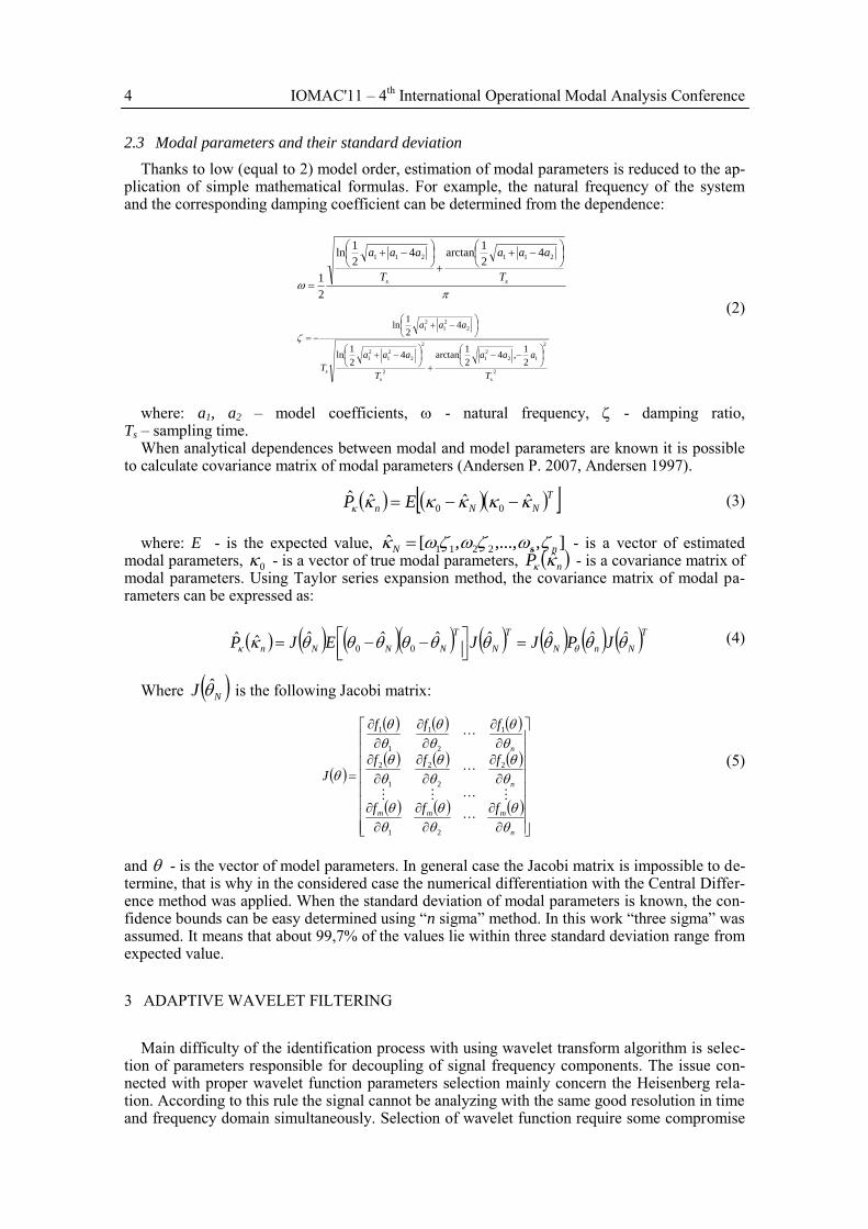
In the presented algorithm, the scale parameter ai is determined based on the frequency fi es-timated from recursive model.

Figure 4: Scheme of adaptive procedure organization. Adaptation process is realized by comparing wavelet frequency and frequency obtained from

RLS algorithm. If the frequencies have the same value or their difference contain in given range, identification process is continued without any changes, but if this two frequencies have different value or their difference has value greater than assumed, the frequency of wavelet function is changed to value corresponding to frequency value estimated from RLS algorithm. Schematically, process adaptation and diagram of method with adaptive wavelet filtering is pre-sented in Figure 4, where fe and fw are current estimated frequency and wavelet frequency re-spectively.

4 HARDWARE IMPLEMENTATION OF MODAL PARAMETERS TRACKING ALGORITHM

The time-domain method, based on classical recursive RLS algorithm, is applied as the pro-posed solution and is efficient enough and relatively easy to implement. The idea of the pro-posed method is based on application of wavelets filtering for decomposition of measured sys-tem response into components related to particular vibration modes. These components can be extracted in parallel way for all modes. The procedure can be applied to any number of meas-ured signals and consists of steps listed in the diagram (Figure. 5b).

dt

a

btgtx

abaxW

i

iiii

i

iiiig

*1,

i

si

a

Tf

6 IOMAC'11 – 4th International Operational Modal Analysis Conference

)()()(=)()()()( tFtFtFtKtGAtM tca qqq

tq

tq

tq

tZ

=)(

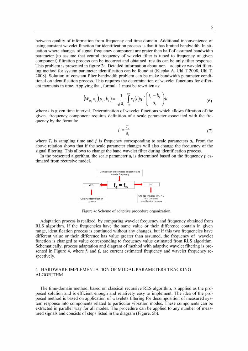
The hardware architecture is shown diagrammatically in Figure 5a. In proposed solution hard-ware is limited to two analog inputs and A/D signal conversion with 200 Hz sampling rate and two analog outputs with value of natural frequency and damping ration for chosen normal mode. a) b)

Figure 5 : Hardware implementation: a) Scheme of implemented hardware, b) Diagram of applied pro-cedure

The USB digital output is implemented to present results for all investigated vibration modes. Used FPGA Altera chip helps to monitor maximum 60 modes simultaneously on-line within 5 ms period.

5 CASE STUDIES

5.1 An aero – elastic model

The aeroelastic equations define the time evolution of the vector )(tq of the structure generalized displacements by the second-order differential equation (Klepka A. Uhl T 2008). The left-hand side of this equation concerns the structural efforts while the right-hand side is the sum of various external forces. The vector of the measurements )(tZ depends linearly on )(tq and its first and second derivatives according to equation :

(8)

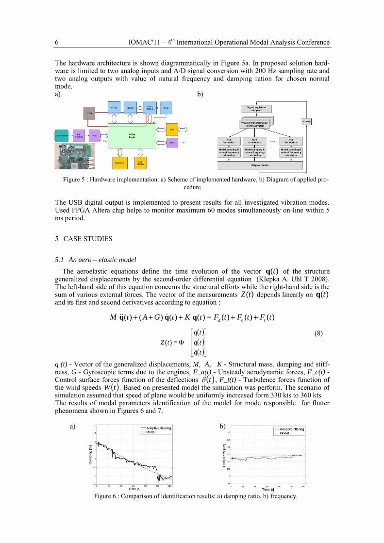
q (t) - Vector of the generalized displacements, M, A, K - Structural mass, damping and stiff-ness, G - Gyroscopic terms due to the engines, F_a(t) - Unsteady aerodynamic forces, F_c(t) - Control surface forces function of the deflections t , F_t(t) - Turbulence forces function of the wind speeds tW . Based on presented model the simulation was perform. The scenario of simulation assumed that speed of plane would be uniformly increased form 330 kts to 360 kts. The results of modal parameters identification of the model for mode responsible for flutter phenomena shown in Figures 6 and 7. a) b)

Figure 6 : Comparison of identification results: a) damping ratio, b) frequency.

7

a) b)

Figure 7 : Identified time history of modal parameters non – stationary aero - elastic system with esti-mated confidence bounds: a) damping ratio, b) natural frequency..

As can be noticed some peaks appeared in estimated confidence bounds. This occurrence is

caused by wavelet adaptation process. In the next step after wavelet function changing, the RLS algorithm is called with initial parameters connected with “old” wavelet function. As a result of it covariance matrix values increase temporary. This problem was solved in hardware version where parallel computation can be perform.

5.2 System with variable stiffness

The hardware implementation of algorithm was tested on the 1DOF system with variable stiff-ness. Experimental setup of experiment is presents in Figure 8.

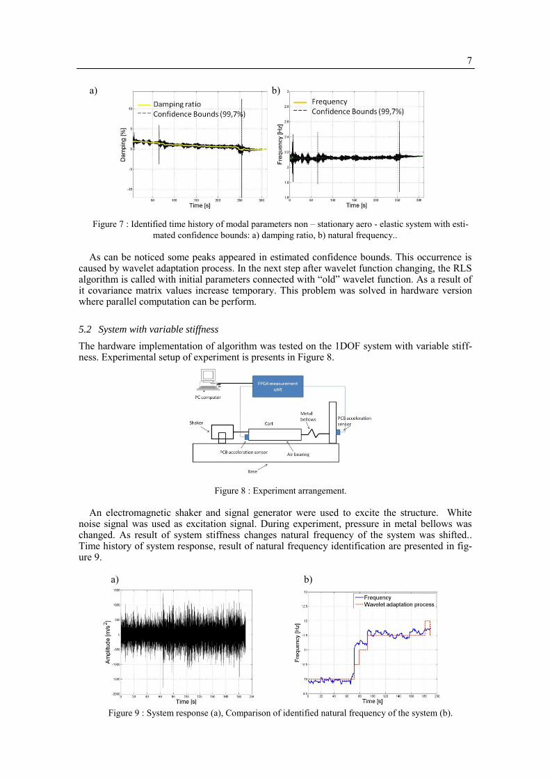
Figure 8 : Experiment arrangement. An electromagnetic shaker and signal generator were used to excite the structure. White

noise signal was used as excitation signal. During experiment, pressure in metal bellows was changed. As result of system stiffness changes natural frequency of the system was shifted.. Time history of system response, result of natural frequency identification are presented in fig-ure 9.

a) b)

Figure 9 : System response (a), Comparison of identified natural frequency of the system (b).

8 IOMAC'11 – 4th International Operational Modal Analysis Conference

Additionally, wavelet adaptation process was presented in Figure 9b (red dashed line).

6 CONCLUSIONS

All performed test showed that adaptive wavelet formula combined with RLS algorithm gives satisfactory results. Natural frequency of the systems are identified much better then damping ratios. Good results of natural frequency identification gives a possibility of use this kind of algorithm in other applications. An example can be vibrating string sensors where fre-quency of oscillation of sensor resonator can give information about changes of operational condition. Another example can be process of rotational speed tracking in structures like wind turbine, gear boxes or mining machines. A formulated algorithm allows computing modal pa-rameters of structures in real – time. Hardware implementation of the algorithm is proposed with the Hardware-Software Co-design approach, i.e. a part realized by hardware and the re-maining part by software running on a Nios II soft-processor contained in the FPGA. Using adaptive formula of wavelet filter, process of wavelet function selection was simplified. The method enable to track modal parameters of the non – stationary system even if their changes are significant.

REFERENCES

Andersen P., Brincker R., Goursat M., Mevel L., 2007. Automated Modal Parameter Estimation For Operational Modal Analysis of Large Systems, Proceedings of the 2nd International Operational Modal Analysis Conference (IOMAC),. Andersen, P., 1997, Identification of Civil Engineering Structures using Vector ARMA Models, Aalborg University. Brenner M.J., R.C. Lind and D.F. Voracek , 1997, Overview of recent flight flutter testing research at NASA Dryden, NASA TM/4792. Brenner, M. J., 2003, Non-stationary dynamics data analysis with wavelet-SVD filtering, Mechanical Systems and Signal Processing, 2003: 765–786. Cooper, A.A. Abbasi and J.E., 2006, Current Status and Challenges for Flight Flutter Testing, Proceedings of ISMA 2006 Conference,: 1523- 1546. Kehoe, M.W., 1995, A historical Preview of flight flutter testing, AGARD Conference Proceedings 566, Advanced Aeroservoelastic Testing and Data Analysis,: 1–15. Klepka A. Uhl T, Vacher P., 2008, On-line flight flutter margin detection—algorithm and case study, Structural health monitoring: proceedings of the fourth European workshop, 2008: 1249–1256. Reed, I.E. Garrick and W.H. "Historical development of aircraft flutter." Journal of Aircraft, 1981: 897-912. Uhl T, Klepka A., 2005, Application of wavelet transform for identification of modal parameters of nonstationary systems, Journal of theoretical and applied mechanics, 2005: 277 – 296. Uhl T., Klepka A., 2006, The use of wavelet transform for in-flight modal analysis XII International Conference on Noise and Vibration Engineering,. Uhl T., Petko M. , Karpie Gl, Klepka A., 2008, Real time estimation of modal parameters and their quality assessment, Shock and Vibration,: 299–306. Verboven P., B. Cauberghe, P. Guillaume, S. Vanlanduit, E. Parloo., 2004, Modal parameter estimation and monitoring for on-line flight flutter analysis, Mechanical Systems and Signal Processing,: 587–610.