Embed Size (px)
Citation preview

REAL-TIME CONTROL OF CYCLING IN A HIGH-PERFORMANCE LEG
WITH SERIES-ELASTIC ACTUATION
A Thesis
Presented in Partial Fulfillment of the Requirements for
the Degree of Bachelor of Science with Distinction
at The Ohio State University
By
Paul Birkmeyer
* * * * *
The Ohio State University
2007
Honors Examination Committee: Approved by:
Dr. David E. Orin
Dr. James P. Schmiedeler ________________________________
Adviser Electrical and Computer Engineering


iii
CONTENTS Page
Abstract………………………………………………………………………………….....v
Acknowledgments………………………………………………..……………..………...vi
List of Figures…………………………………….…………………..…..…………..…...vii
List of Tables……………………………………………………………………………..viii
Chapters:
1. INTRODUCTION ............................................................................................................... 1
1.1 Background.......................................................................................................... 1
1.2 Previous Research................................................................................................ 5
1.3 Research Objectives ............................................................................................ 6
1.4 Thesis Organization............................................................................................. 7
2. IMPROVEMENTS TO EMBEDDED SYSTEM CONTROLLER.................................. 9
2.1 Introduction.......................................................................................................... 9
2.2 Hardware Integration of Potentiometer ............................................................ 10
2.2.1 Manipulation of Input Pins.............................................................................. 11
2.2.2 Maximizing Angular Resolution..................................................................... 13
2.3 Software Integration of Knee Potentiometer .................................................... 16
2.3.1 Changes to the KoreMotor Code .................................................................... 17
2.3.2 Changes to the KoreBot Code......................................................................... 21
2.3.3 Applications of Direct Knee Angle Sensing................................................... 24
2.4 Summary............................................................................................................ 29
3. IMPLEMENTATION OF HIGH-SPEED CYCLING .................................................... 30
3.1 Introduction........................................................................................................ 30
3.2 Inverse Kinematics ............................................................................................ 30
3.3 Cubic Spline Generation ................................................................................... 33
3.4 Cycling Algorithm............................................................................................. 35
3.5 Results................................................................................................................ 38
3.6 Summary............................................................................................................ 45

iv
4. SUMMARY AND CONCLUSIONS ............................................................................... 46
4.1 Summary and Conclusions................................................................................. 46
4.2 Future Work........................................................................................................ 47
Appendices:
Appendix A1: Values for Physical Parameters of Leg [1]...................................... 50
Appendix A2: Integration of Foot Contact Sensing to DIP Switch........................ 51
Appendix A3: Integration of Analog-to-Digital Conversion on the KoreMotor
Board ......................................................................................................................... 52
Appendix A4: New I2C Feedback Protocol ............................................................ 53
Appendix A5: New kmot_AdvancedReadHip Function......................................... 55
Appendix A7: Safety Routines Added to the KoreMotor Board ............................ 59
Appendix A8: Computation of Inverse Kinematics and Inverse Jacobian............. 61
Appendix A9: Cubic Spline Functions and Derivations ......................................... 65
Appendix A10: Cycle Function................................................................................ 67
Appendix A11: Getting System Time on the KoreBot ........................................... 75
v
ABSTRACT
A high-performance, lightweight prototype robotic leg using series-elastic
actuation was developed in previous work to study the effects of series-elastic actuation
in vertical jumping. However, there was also a desire to perform other high-speed
dynamic motions with the leg such as cycling. To this end, the thesis goals were focused
on improving the existing embedded controller as well as implementing a high-speed
cycling function. An analog potentiometer was used to replace a faulty sensor at the knee
joint, which houses the compliant element of the series-elastic actuator. Changes were
made to the previous controller hardware and software in order to utilize the data
available from this new sensor. Using several new functions, a smooth cyclical trajectory
was created and followed by the robotic leg at high speeds. The entire cycle was
completed in less than 0.5 seconds with a stroke of more than 15cm. These functions will
open the path for development of precise trajectory control in future robotic legs, as well
as allow for the study of series-elastic actuation through a new dynamic motion. The
design of the aforementioned changes and functions are discussed. The significance of
the thesis results is discussed, as well as the expected course of future work.

vi
ACKNOWLEDGMENTS
My most sincere thanks go to Simon Curran for his generous offerings of time,
wisdom, and support through all of the issues that arose during this project. His patient
teachings proved invaluable in coming up to speed on the intricacies of the entire system.
Po-Kai Huang was a great mentor, and he deserves many thanks as well. Even
after he returned home to Taiwan, he was more than willing to help debug the system. He
had an incredible ability to get to the root cause of a problem, and I hope to learn from
him.
My sincere thanks also go to Alexis Weitner for her countless hours proofreading
my documents, practicing my presentations, designing figures, and providing tireless
mental support.
I would also like to thank Dr. Orin and Dr. Schmiedeler for their incredible
patience and understanding through this hectic process.

vii
LIST OF FIGURES
Figure Page
Figure 1.1: Articulated Jumping Leg [1] 1
Figure 1.2: Block Diagram for Generic Series Elastic Actuator [1] 2
Figure 1.3: K-Team KoreBot Front (Right) and Back (Left) [6] 3
Figure 1.4: K-Team KoreMotor Front (Bottom) and Back (Top) [7] 4
Figure 1.5: Communication Hierarchy of Control System [1] 5
Figure 2.1: KoreMotor Motor Port Pins [7] 11
Figure 2.2: Modification to DIP Switch for Foot Contact Sensing on KoreMotor 13
Figure 2.3: Biasing of Knee Potentiometer Relative to Thigh 15
Figure 2.4: Consolidation to Three PICs 19
Figure 2.5: Flowchart of new_i2c_prepare_data Function for the Hip PIC 21
Figure 2.6: Angle of Knee Computed by the Knee Encoder vs. the Angle Computed by
the Hip Encoder and Knee Potentiometer 26
Figure 2.7: Spring Deflection During Two Consecutive Jumps 27
Figure 3.1: Coordinate System for Inverse Kinematics and Inverse Jacobian 31
Figure 3.2: Flowchart of Cycling Algorithm 35
Figure 3.3: Generated Cubic Spline From Reference Points 39
Figure 3.4: Actual Motion vs. Commanded Motion for One Cycle 41
Figure 3.6: Knee Motor Encoder Position vs. Commanded Position for Three Cycles 43
Figure 3.7: Foot Trajectory Consistency Over 10 Cycles 45
Figure A1.1: Physical Representation of Leg 50

viii
LIST OF TABLES
Table Page
Table 2.1: Comparison of I2C Communication for Data Feedback................................. 24
Table A1.1: Physical Leg Parameters ............................................................................ 50

1
CHAPTER 1
INTRODUCTION
1.1 Background
This project mainly focuses on establishing the ability to perform high-speed
cycling on a high-performance, series-elastic leg while simultaneously improving its
ability to perform feedback sensing. Since 2003, a lightweight, real-time computer-
controlled, series-elastic, articulated jumping leg has been under development at The
Ohio State University. The team working on its development is headed by Dr. David E.
Orin of the Department of Electrical and Computer Engineering and Dr. James P.
Schmiedeler of the Department of Mechanical Engineering at The Ohio State University.
This prototype leg, seen in Figure 1.1, was designed to study the capabilities required for
jumping, quadruped galloping, and dynamic locomotion in general [1,2]. A more detailed
overview of the system, including lists of physical dimensions, can be seen in Appendix
A1.
Figure 1.1: Articulated Jumping Leg [1]

2
The leg was designed by Joseph Remic III [2] under Dr. Schmiedeler in order to
investigate a lightweight leg with series-elastic actuation for use in a galloping
quadruped. Simon Curran, under Dr. Orin, performed the integration of motors,
amplifiers, sensors, and control hardware as well as generation of the foundation of
software from which this research is built [1]. The entire system is constrained from
lateral movement by vertical guide rails. All of the control hardware is located on the top
of the leg, with only the power supply located outside of the platform.
Series-elastic actuation in its most fundamental form can be seen in Figure 1.2. This
type of actuation is present in the knee joint of the robotic leg with the intention of
allowing energy storage to be used in vertical jumping [1,3]. Series-elastic actuation also
has the benefits of reducing impact forces at the load as seen by the actuator [1,4].
However, because the actuator is not directly connected to the load, the system is unable
to directly determine the load position based solely on the actuator position due to the
compliance in the series-elastic actuation [1]. Thus, in order to directly measure the knee
angle, a separate sensor must measure the knee joint angle itself rather than relying on the
position feedback of the knee actuator.
ACTUATOR LOAD
SERIESELASTICITY
Figure 1.2: Block Diagram for Generic Series Elastic Actuator [1]
Given that this leg was developed to perform high-speed motions, with specific
attention given to vertical jumping, the system was designed to be as lightweight as
possible in order to achieve the greatest possible height. However, the desire was also to
3
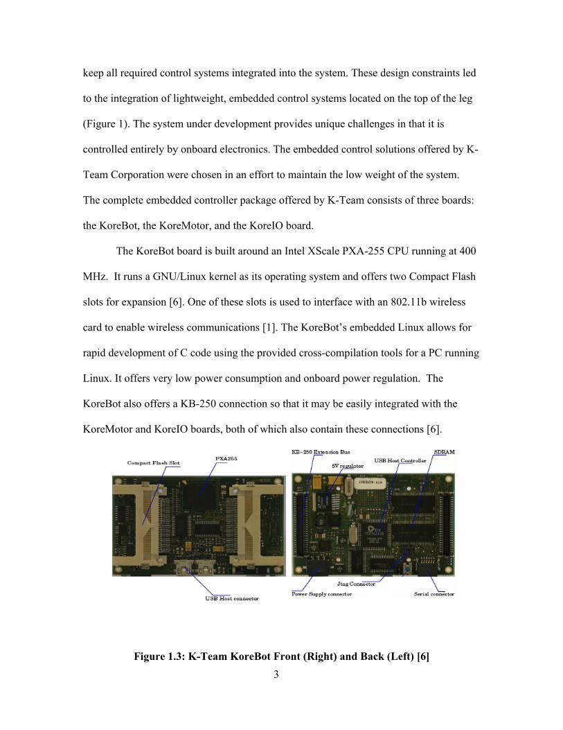
keep all required control systems integrated into the system. These design constraints led
to the integration of lightweight, embedded control systems located on the top of the leg
(Figure 1). The system under development provides unique challenges in that it is
controlled entirely by onboard electronics. The embedded control solutions offered by K-
Team Corporation were chosen in an effort to maintain the low weight of the system.
The complete embedded controller package offered by K-Team consists of three boards:
the KoreBot, the KoreMotor, and the KoreIO board.
The KoreBot board is built around an Intel XScale PXA-255 CPU running at 400
MHz. It runs a GNU/Linux kernel as its operating system and offers two Compact Flash
slots for expansion [6]. One of these slots is used to interface with an 802.11b wireless
card to enable wireless communications [1]. The KoreBot’s embedded Linux allows for
rapid development of C code using the provided cross-compilation tools for a PC running
Linux. It offers very low power consumption and onboard power regulation. The
KoreBot also offers a KB-250 connection so that it may be easily integrated with the
KoreMotor and KoreIO boards, both of which also contain these connections [6].
Figure 1.3: K-Team KoreBot Front (Right) and Back (Left) [6]
4
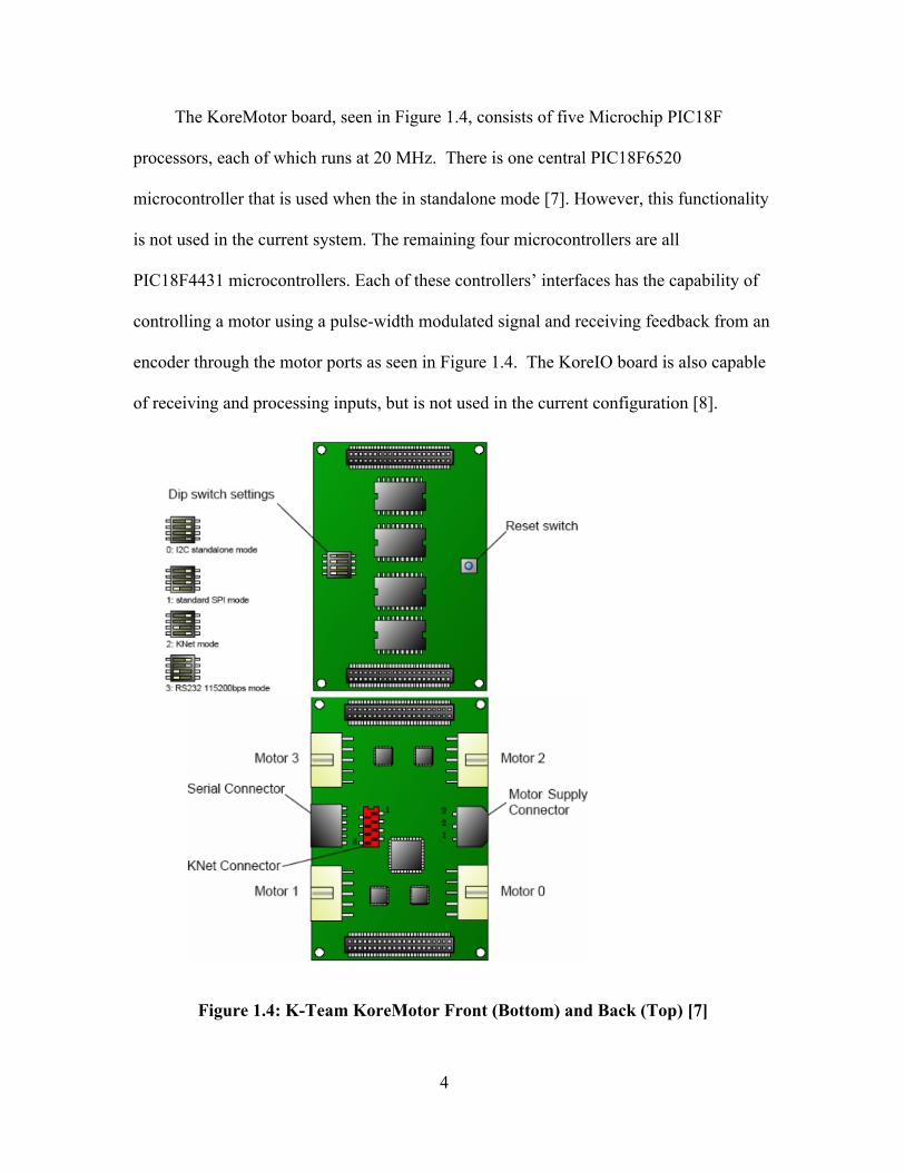
The KoreMotor board, seen in Figure 1.4, consists of five Microchip PIC18F
processors, each of which runs at 20 MHz. There is one central PIC18F6520
microcontroller that is used when the in standalone mode [7]. However, this functionality
is not used in the current system. The remaining four microcontrollers are all
PIC18F4431 microcontrollers. Each of these controllers’ interfaces has the capability of
controlling a motor using a pulse-width modulated signal and receiving feedback from an
encoder through the motor ports as seen in Figure 1.4. The KoreIO board is also capable
of receiving and processing inputs, but is not used in the current configuration [8].
Figure 1.4: K-Team KoreMotor Front (Bottom) and Back (Top) [7]

5
The K-Team control system uses Inter-Integrated Circuit (I2C) communications, a
serial communication protocol developed by Philips, as an interface between the KoreBot
and each microcontroller on the KoreMotor board through the KB-250 interface [7]. Each
microcontroller on the KoreMotor board is assigned a unique I2C address so that the
KoreBot may communicate with each chip individually [7]. In order to achieve any sort
of dynamic motion or feedback, the KoreBot board sends or receives data through the I2C
bus. A simple control architecture diagram is shown in Figure 1.5 that illustrates the
control flow of a single motor. An in-depth discussion of the interface between the K-
Team control system and the physical actuators and sensors has been written before [1].
Figure 1.5: Communication Hierarchy of Control System [1]
1.2 Previous Research
Simon Curran, a graduate student under Dr. Orin, has been working with the
robotic leg and control system for several years. His efforts were directed to performing,
and then optimizing, vertical jumping with the robotic leg. His work has shown that the
performance of a vertical jump can depend largely upon the proper utilization of the

6
series-elastic actuation in the knee motor [1]. However, in the course of running
experiments with the robotic leg, the sensor used to measure the angle of the knee joint
directly furnished erroneous data. This made it impossible to determine the direct knee
joint angle as well as the state of the spring in the series-elastic actuator. Curran also
expressed the desire to study different high-speed dynamic motions, specifically those
that can be applied to legged locomotion [1]. However, due to the complexity of the
system and the amount of time required to develop a full understanding of vertical
jumping with a series-elastic actuator, no other high-speed motions were really explored.
1.3 Research Objectives
The main objective of this work is to continue the efforts towards the creation of
high-speed, dynamic motions while maintaining real-time feedback of the robotic leg.
This includes developing a high-speed cycling motion in which the leg is suspended in
mid-air as well as developing a new method for direct sensing of the knee angle.
In order to successfully replace the previous knee angle sensor and obtain tenable
data, a good replacement sensor first needed to be selected. Successful integration of the
sensor into the hardware system was critical to ensure accurate and reliable
measurements. The software on the KoreMotor microcontrollers needed to be modified in
order to properly sense the knee angle, process the data internally, and communicate it
with the KoreBot. The KoreBot needed to be able to process this incoming data properly
as well. It also had to be able to correlate these values to physical angles of the knee joint.
All of these measurements and communications should be realized as quickly as possible
in order to be able to maintain real-time control.

7
To achieve high-speed cycling controlled in real-time, several new functions
needed to be developed. The leg had to be able to generate smooth trajectories from a
limited set of inputs so that user input could be kept as minimal as possible. These
trajectories needed to be based in Cartesian coordinates in order to maintain the most
intuitive interface possible. Finally, a function that integrated these abilities with the
ability to track the system, issue new commands and obtain system feedback in real-time
is needed to successfully implement a high-speed cycling motion.
1.4 Thesis Organization
Chapter 1 of this thesis presents background information on the project aimed at
studying a high-performance, lightweight, series-elastic actuated prototype robotic leg.
Key features of the physical system are discussed, as well as a more in-depth discussion
of the embedded controller. Next, a summary of previous work done on the robotic leg is
discussed along with problems and shortcomings that were determined as a result of that
research. Finally, a summary of the research objectives of this project is presented.
Chapter 2 will focus on the improvements made to the embedded controller of the
robotic system. The addition of a potentiometer at the knee joint will be discussed, going
into detail regarding the physical changes to the embedded controller circuitry in addition
to software changes on both the KoreMotor and KoreBot systems. Chapter 2 concludes
with the results from these improvements, including communication optimizations,
spring deflection measurement, and safety routine implementations.
Chapter 3 will discuss the development of a cycling algorithm. First, a means of
computing the inverse kinematics and inverse Jacobian, used to compute the joint angle

8
and their rates, will be described. Then, a function that computes cubic spline
interpolations between two points will be shown in detail. A third function capable of
utilizing the previous two functions to generate cyclical motions through which the
robotic leg is controlled in real-time will be discussed. Finally, the results from a
performance of high-speed cycling using these functions are analyzed.
Finally, Chapter 4 is a summary with conclusions of the research performed in
this thesis. It also provides recommendations for future study and applications.
9
CHAPTER 2
IMPROVEMENTS TO EMBEDDED SYSTEM CONTROLLER
2.1 Introduction
This chapter will discuss the improvements made to the embedded system
controller used for real-time control of the robotic leg. The focus of the chapter will lie
specifically in the addition of the ability to directly sense the knee joint angle and the
resulting improvements that derive from the process of integrating and utilizing such an
improvement. The applications possible by sensing the direct knee angle are very
exciting and can lead to new developments in safety routines, spring deflection analysis,
and energy analysis of the system during dynamic motions.
In order to directly sense the angle between the thigh and shank of the robotic leg,
a sensor is needed directly on the knee joint itself. Due to the series-elastic actuation of
the shank, the knee motor is unable to directly determine the angle of the shank relative
to ground. Any deflection of the spring in the knee joint leads to a discrepancy between
the perceived angle of the shank as determined by the knee motor encoder and the actual
angle of the shank. The only way to become aware of an actual discrepancy is to measure
the knee joint angle directly.
This sensing was previously done with a rotary encoder manufactured by Gurley
Precision Instruments that was dedicated to the knee joint [1]. However, due to the
inability of this encoder to withstand the extreme forces experienced during jumping as
well as its susceptibility to electromagnetic noise, it was not a viable means of
determining the knee angle directly.

10
A potentiometer was a practical replacement to the Gurley encoder. A
potentiometer would be more robust in the face of high forces and torques and was less
prone to corruption by electromagnetic noise. The resistance of the potentiometer needed
to be adequately high so that the current draw would be fairly low, keeping the power
consumption low. A CLAROSTAT 308-N-PC-5 potentiometer was chosen as the
substitute. It has a resistance of 5 kilohms and is encased in a plastic housing to reduce
electromagnetic interference within the device. It also weighs 5 grams, thus helping to
keep the weight of the system as small as possible.
2.2 Hardware Integration of Potentiometer
Brian Knox, an undergraduate Mechanical Engineering student working on the
robotic leg, physically mounted the potentiometer on the system [9]. However, hardware
modifications to the embedded system itself were required in order to integrate the
potentiometer fully into the system. The potentiometer represented an entirely different
type of input signal to the embedded controller than had been previously provided by the
Gurley encoder. The Gurley encoder utilized the digital quadrature encoder input that the
KoreMotor board utilizes. The potentiometer, in contrast, was only capable of providing
an analog voltage signal. Unfortunately, there was no method for directly measuring
analog values on the KoreMotor board. The KoreIO board is capable of reading analog
values, but is not suitable for measuring the knee joint angle. The reasons for avoiding
the use of the KoreIO board and demanding the use of the KoreMotor board for analog
readings will be explained in Section 2.3.

11
2.2.1 Manipulation of Input Pins
The KoreMotor board was not designed to allow for analog signal inputs. Since
all of the pins of the PIC microcontrollers on the KoreMotor are tied directly into the
printed circuit board of the KoreMotor board, the options for pin access are extremely
limited. Fortunately, there is a single pin that is available through the motor encoder input
ports on the KoreMotor seen in Figure 2.1. This pin, which connects to the RA2/INDX
pin on the associated PIC18F4431 chip on the KoreMotor [10], was designed by K-Team
to utilize the motor encoder index output from a motor encoder. The encoder index is
used to allow the encoder to determine absolute positioning using the index as a
reference. The previous hardware setup did not utilize absolute position sensing but
instead used relative positioning [1]. Given that the index pin was not being used in the
previous system, it was instead used as the foot contact input. Unfortunately, the INDX
pin is the only pin that is capable of reading analog inputs and is available with little
modification to the KoreMotor board itself.
Figure 2.1: KoreMotor Motor Port Pins [7]
In order to gain access to the INDX pin, the foot contact sensor would have to be
relocated. This modification was made more difficult because it suffered from the same
lack of available pins as was the case with the analog input. One of the only available
digital inputs that was suitable for the foot contact switch was found in a dual in-line
12
package (DIP) switch on the KoreMotor board. This DIP switch was used within the code
on the microcontrollers to establish a suitable range of addresses for I2C communications
[7]. Since the I2C addressing was never something that needed to be changed during
normal operation, the I2C range could simply be set in software on the microcontrollers
on the KoreMotor.
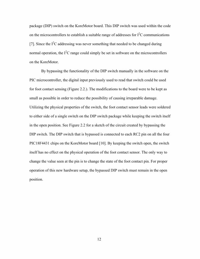
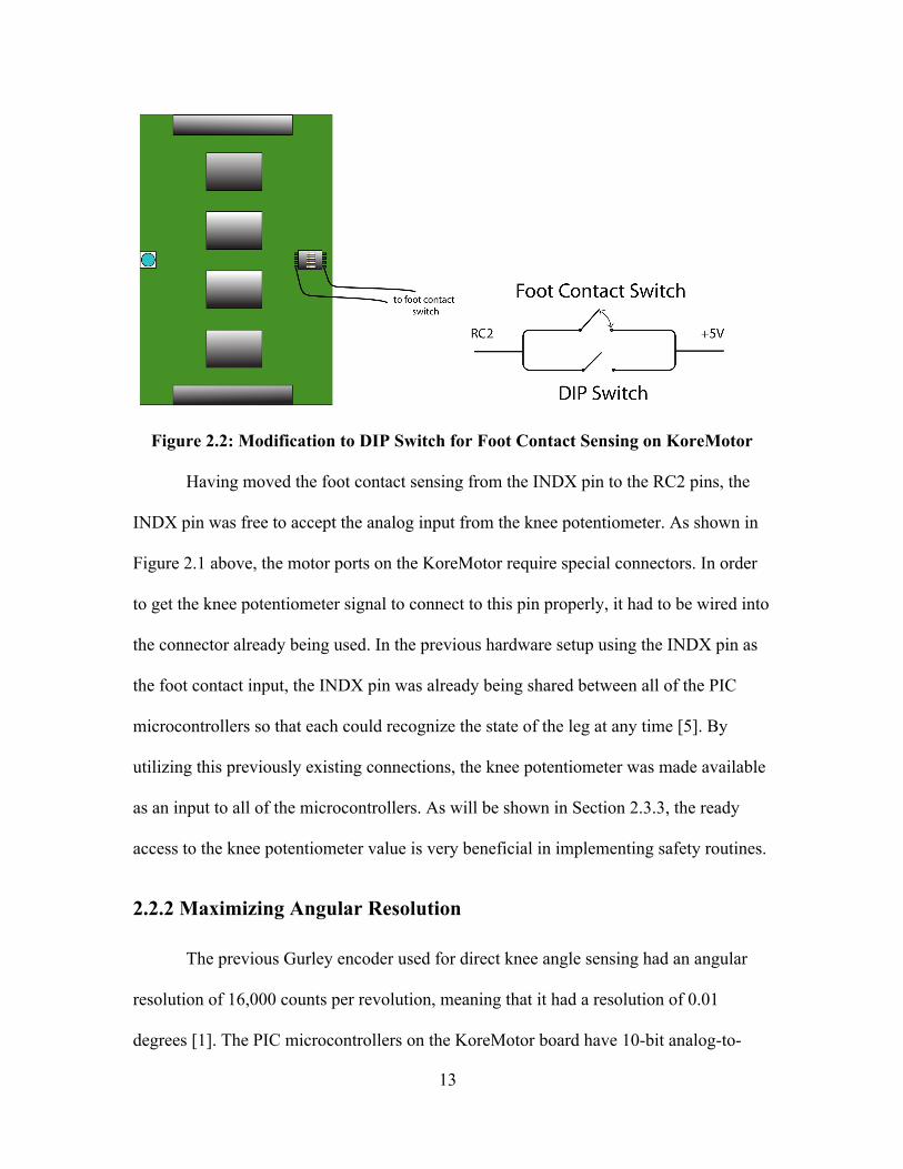
By bypassing the functionality of the DIP switch manually in the software on the
PIC microcontroller, the digital input previously used to read that switch could be used
for foot contact sensing (Figure 2.2.). The modifications to the board were to be kept as
small as possible in order to reduce the possibility of causing irreparable damage.
Utilizing the physical properties of the switch, the foot contact sensor leads were soldered
to either side of a single switch on the DIP switch package while keeping the switch itself
in the open position. See Figure 2.2 for a sketch of the circuit created by bypassing the
DIP switch. The DIP switch that is bypassed is connected to each RC2 pin on all the four
PIC18F4431 chips on the KoreMotor board [10]. By keeping the switch open, the switch
itself has no effect on the physical operation of the foot contact sensor. The only way to
change the value seen at the pin is to change the state of the foot contact pin. For proper
operation of this new hardware setup, the bypassed DIP switch must remain in the open
position.
13
Figure 2.2: Modification to DIP Switch for Foot Contact Sensing on KoreMotor
Having moved the foot contact sensing from the INDX pin to the RC2 pins, the
INDX pin was free to accept the analog input from the knee potentiometer. As shown in
Figure 2.1 above, the motor ports on the KoreMotor require special connectors. In order
to get the knee potentiometer signal to connect to this pin properly, it had to be wired into
the connector already being used. In the previous hardware setup using the INDX pin as
the foot contact input, the INDX pin was already being shared between all of the PIC
microcontrollers so that each could recognize the state of the leg at any time [5]. By
utilizing this previously existing connections, the knee potentiometer was made available
as an input to all of the microcontrollers. As will be shown in Section 2.3.3, the ready
access to the knee potentiometer value is very beneficial in implementing safety routines.
2.2.2 Maximizing Angular Resolution
The previous Gurley encoder used for direct knee angle sensing had an angular
resolution of 16,000 counts per revolution, meaning that it had a resolution of 0.01
degrees [1]. The PIC microcontrollers on the KoreMotor board have 10-bit analog-to-
14
digital conversion (ADC) capabilities, meaning that the resolution is limited to 1024
divisions over the voltage range accepted by the microcontrollers [10]. The closed
hardware system of the KoreMotor board had tied the reference voltages of the
KoreMotor PIC microcontrollers to 0V and 5V, thus limiting the acceptable range of
input values from the knee potentiometer to 0V through 5V. This means that the ADC on
the microcontrollers can only recognize differences in (5-0) V/1024, or roughly 0.005V.
The best way to maximize the angular resolution for the knee joint angle to is to
maximize the voltage range of the potentiometer within the 5V range accepted by the
microcontrollers. This means that the potentiometer must be set up so that there is a
voltage range of 0 through 5V through the entire range of motion of the knee angle. This
was done as shown in Figure 2.3. The potentiometer has a range of rotation of
approximately 300 degrees, while the knee has a range of approximately 120 degrees. By
putting 12VDC across the entire range of the potentiometer from the PT4313 power
supply [1], approximately 4.7VDC was seen across the range of motion. The
potentiometer is fixed relative to the thigh, so only changes of the shank relative to the
thigh is measured. The potentiometer was oriented such that there is a range of
approximately 5 degrees prior to the shank reaching singularity in which the
potentiometer outputs zero degrees throughout. This is done to make sure that the leg
does not, in fact, leave the proper range of operation and send a signal greater than 5V to
the KoreMotor board. Thus, out of a possible 1024 steps of resolution available, the knee
angle can utilize approximately 975 steps of resolution. Thus, the knee angle
potentiometer and the PIC microcontrollers are able to resolve differences in knee angle
of approximately 0.12 degrees.

15
Figure 2.3: Biasing of Knee Potentiometer Relative to Thigh
This resolution is poorer than was possible with the Gurley encoder, but it was
deemed adequate for the robotic leg. Unfortunately, the potentiometer analog signal line
suffers from noise much as the Gurley encoder did. The source of the noise is currently
unknown, but it introduces noise roughly on the scale of 15 or 20 millivolts. This
translates to a fluctuation of half a degree on either side of the actual value. This amount
of noise is unacceptable for controlling the leg through the knee angle, but it is sufficient
to get approximate values of the knee angle.
There are several possible sources of noise that need to be explored in order to
reduce the noise that is present on the analog line of the knee potentiometer. The 12VDC
supply that biases the potentiometer comes from the PT4313 power supply. Any
fluctuation on the output voltage of the supply would affect the biasing of the
potentiometer, thus affecting the voltage level at the PIC ADC pin. Fluctuations of
approximately 36 to 48 millivolts at the terminals of the supply would be required to

16
create the noise levels that are seen on the signal line. Another possible source of noise
could come from the reference voltage supplies on the KoreMotor boards. The reference
voltage lines used to by the ADC on the PIC microcontrollers are tied to the board itself,
and any fluctuation on those lines could change the value given by the ADC. The third
possible source of noise would be from electromagnetic noise present in the
electromechanical system. The current signal, ground and 12V lines are twisted together
in an attempt to reduce the effects of electromagnetic radiation, but that is certainly not a
guaranteed fix. All that is known at this point is that there are still significant amounts of
noise on the knee potentiometer line that remains to be explained definitively.
2.3 Software Integration of Knee Potentiometer
This section will address the changes to the software of the embedded system in
order to utilize the feedback information made possible by including the knee
potentiometer in the robotic leg. Changes were required in the software on both the
KoreMotor board as well as on the KoreBot board. All changes made on the KoreMotor
board were done in the Windows XP environment using the Custom Computer Services,
Inc. PCWH C-compiler. All changes for the KoreBot board were made in the Linux
environment using the LibKoreBot Application Programming Interface (API) provided
by K-Team as well as the new updated API commands created by Simon Curran and Po-
Kai Huang [1,5].

17
2.3.1 Changes to the KoreMotor Code
2.3.1.1 Accommodating New Input Pins
As discussed in an earlier section, the previous input for the foot contact sensing
was a digital input sensed on the INDX pin of the motor encoder ports. The relocation of
the foot contact sensing input to the new pin location required several changes in the code
on the PIC microcontrollers on the KoreMotor board. It required defining a new pointer
entitled c_CONTACT_PIN that could be referenced instead of the previous pointer used
for the INDX pin. Appendix A2 shows how the foot contact pin pointer was changed and
how it can be used to retrieve the input of the foot contact sensor. Most importantly, the
new pointer had to be used in every I2C protocol in order to send the proper foot contact
status to the KoreBot to allow for proper control during jumping.
Relocating the foot contact switch input to a different pin left the INDX pin open
for the new analog input. Since the pin was previously used as a digital input, it required
changing the initialization routine created by K-Team in the controler.c file. The code
showing the proper initialization using the new pointer mentioned above can be seen in
Appendix A2 as well. The change was a simple change to one of the registers in the PIC
microcontroller responsible for controlling the type of input present on each pin capable
of receiving analog inputs.
2.3.1.2 Analog-to-Digital Conversion
In order for a PIC microcontroller to be able to properly process an analog input,
it was necessary to convert the analog value to a digital value. The PIC18F4431
microcontrollers on the KoreMotor each have 10-bit analog-to-digital converters (ADCs)
capable of doing conversions of analog signals without using CPU resources [10]. It

18
simply requires properly initializing the ADC, setting a bit to start the conversion
process, and then waiting for the value to be converted and stored into a register. Each
analog-to-digital conversion takes approximately six microseconds, meaning that the
conversion must be started so that it is known that enough time will pass before the
conversion will be read. The placements of both the ADC trigger and the reading of the
analog value as well as the initialization of the ADC are shown in Appendix A3.
It should be noted that this analog-to-digital conversion can run on each of the
PIC microcontrollers while only negligibly taxing the CPU resources on each. The
required CPU time needed to complete a single conversion is approximately 400
nanoseconds. This allows the previous functionality of the PIC microcontrollers to
continue unabated while simultaneously benefiting from the ability to perform analog-to-
digital conversions.
2.3.1.3 Consolidation of PICs, I2C Communications
Changes were also required for the I2C communication protocol so that the
microcontrollers would simply be able to send the 10-bit value to the KoreBot. As
mentioned previously, it is possible for each PIC microcontroller to process the analog
value from the knee potentiometer simultaneously with the digital encoder input from the
motors or the string potentiometer that measures the body height. Thus, it is possible to
use a single PIC microcontroller to send the information from the knee potentiometer as
well as from a single other digital encoder input. There are several advantages that derive
directly from sending the knee potentiometer value along with all the previous
information sent to a single microcontroller.

19
The first advantage from this approach is that it gives the ability to remove one of
the four PIC microcontrollers from the feedback loop. Whereas previously each PIC was
responsible for only one input, it became possible to incorporate more than one feedback
sensor into a single PIC. See Figure 2.4 for the way in which the actual consolidation was
arranged, combining the knee potentiometer value with the hip motor encoder value. The
first improvement this consolidation would bring immediately is a reduction in the
number of PIC microcontrollers, which need to be addressed in order to gain all feedback
information, from four to three.
Figure 2.4: Consolidation to Three PICs
By carefully choosing which PIC microcontroller would send the direct knee
angle information as well as which microcontroller would be excluded, even larger gains
could made. By some hardware defect in the current KoreMotor board, it has been
impossible to reprogram the PIC that was responsible for the string potentiometer. As a
result, it has not benefited from the I2C optimizations implemented by Po-Kai Huang [5].
Thus, by removing this microcontroller, it could be removed from the feedback loop and

20
greatly increase the speed with which feedback could be accomplished.
The knee potentiometer data was paired with the hip motor PIC microcontroller
for a specific reason as well. Under the condition when there is no spring deflection in the
knee joint, the knee motor encoder gives the angle of the shank relative to the ground [1].
However, if there is spring deflection in the knee joint, the only way to accurately
compute the shank angle relative to the ground is by knowing the hip angle and the direct
knee angle. Thus, by allowing one PIC to return both the hip motor angle and the direct
knee angle, it provides all the information necessary to compute the shank angle. As is
shown in Appendix A3, the hip PIC updates the direct knee angle from the potentiometer
and the hip motor position at nearly the same time instant, assuring that the two values
are nearly simultaneous, giving more accurate shank angle computations.
Consolidating the data feedback to three microcontrollers on the KoreMotor board
demanded that the I2C protocol be extended to allow for the hip PIC to send the knee
potentiometer value along with the foot contact state, the motor position, and the motor
velocity. The changes made to accomplish this follow very closely to the improvements
designed by Huang [5]. Instead limiting the string of data sent in one I2C communication
sequence from the hip PIC to include only the position, velocity, and foot contact state, it
is extended to include two 8-bit data blocks in which the 10-bit ADC value can be placed.
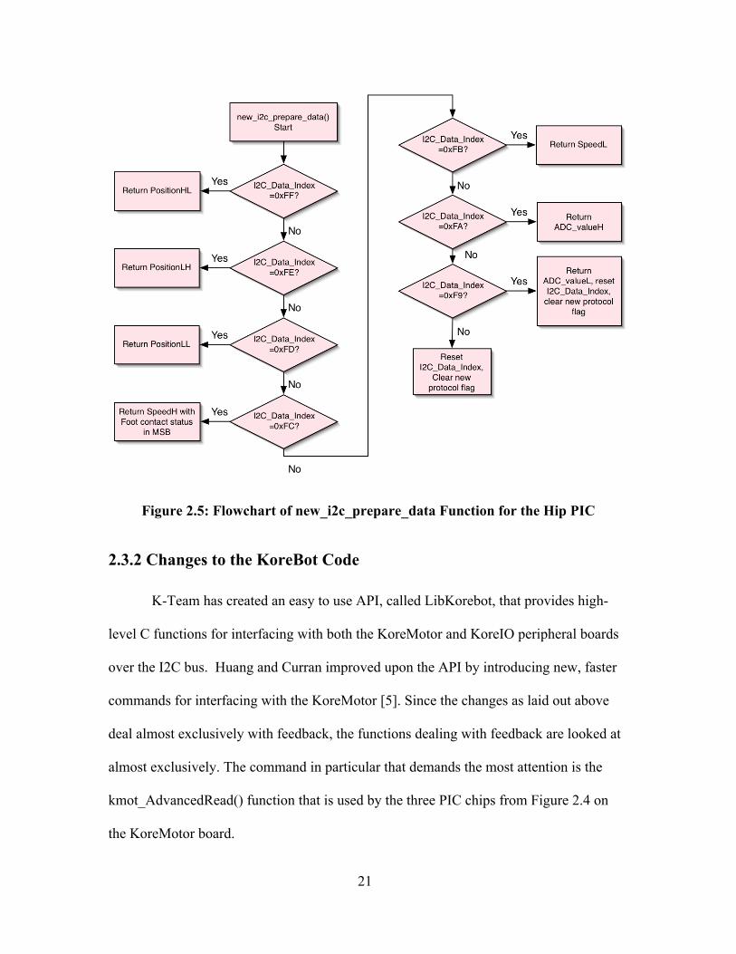
A flowchart showing the operation of the new I2C feedback protocol is shown in Figure
2.5. The resulting new_i2c_prepare_data function on the hip microcontroller that handles
the feedback communications is shown in Appendix A4.
21
Figure 2.5: Flowchart of new_i2c_prepare_data Function for the Hip PIC
2.3.2 Changes to the KoreBot Code
K-Team has created an easy to use API, called LibKorebot, that provides high-
level C functions for interfacing with both the KoreMotor and KoreIO peripheral boards
over the I2C bus. Huang and Curran improved upon the API by introducing new, faster
commands for interfacing with the KoreMotor [5]. Since the changes as laid out above
deal almost exclusively with feedback, the functions dealing with feedback are looked at
almost exclusively. The command in particular that demands the most attention is the
kmot_AdvancedRead() function that is used by the three PIC chips from Figure 2.4 on
the KoreMotor board.

22
The original kmot_AdvancedRead function accepts three pointers that point to memory
locations to hold the values of the position, speed, and foot contact state (Appendix A5).
Since the hip motor is now set up to send the analog value from the potentiometer in
addition to those two things, there must be another pointer added to the accepted
arguments to the kmot_AdvancedRead() command. Rather than modify the existing
kmot_AdvancedRead() command at the risk of corrupting the proper operation of the
original, a new function was created within kmot.c called kmot_AdvancedReadHip() to
handle the I2C feedback communication and processing. It was modeled after
kmot_AdvancedRead(), but features an additional pointer as an argument that points to
the memory location to hold the analog value. Within this function, the I2C
communication buffer length needed to be extended to 7 bytes when calling
knet_readNew() in order to accommodate the extra bytes for the knee potentiometer. See
Appendix A5 for this function along with its declaration in the kmot.h header file.
Consolidating the feedback to three PIC18F4431 microcontrollers and extending
the I2C communication protocol made significant performance gains. Look
at Table 2.1 for a comprehensive comparison of the original K-Team I2C protocol used
[5], the previous iteration based on Po-Kai Huang’s efforts [5], and the most recent
iteration. The table compares different statistics from a complete system feedback
communication loop: the number of I2C operations required; the number of data bytes
sent over the line; the total time required; and the number of interrupts generated on the
PIC microcontrollers. The I2C operations are defined when a new exchange occurs
between the KoreBot and the KoreMotor. When reading data from the KoreMotor board,
the KoreBot must first command a PIC to give the feedback information, and then PIC

23
must give the data in return. These two operations must be performed for each PIC in the
feedback loop; thus, 6 total operations are performed per feedback loop. The number of
data bytes is simply the number of bytes sent over the I2C medium that contain feedback
information. The data bytes that are sent from the knee PIC and the string potentiometer
PIC have not changed from the previous I2C iteration. They send the 24 bits of the
position value first, followed by the 16-bit speed value according to the order established
by Huang [5]. The most significant bit of the speed value is set as the foot contact state
[5]. This creates 5 data bytes for both the knee and the string potentiometer PICs. The hip
PIC, as shown in Figure 2.5, sends these same values in the same order, but then
additionally sends the 10-bit analog value from the knee potentiometer in two 8-byte
blocks. ADC_valueL contains the lower 8 bits while ADC_valueH contains the two most
significant bytes. Therefore, the hip PIC sends 7 additional data bytes, creating a sum
total of 17 data bytes for one feedback loop.
The two most important numbers are the number of interrupts and the total time
delay. Every time an interrupt is generated, a microcontroller must stop what it is
currently doing it in order to process the interrupt. An interrupt occurs on the PIC every
time that a new byte is sent over the I2C protocol. Since every byte generates an interrupt,
sending data more efficiently over the I2C generates fewer interrupts, which in turn
allows the system to focus on the current tasks. The total time delay represents how long
it takes the KoreBot system to gather all of the feedback from the KoreMotor and is
directly related to the number of interrupts generated. When the KoreBot is waiting for
I2C communications to finish, all of its resources are tied and it cannot do other
operations that may be needed. Thus, reductions in feedback times of nearly 50% are
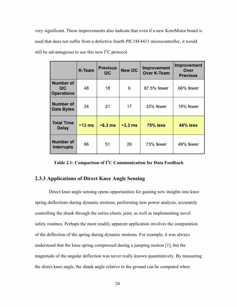
24
very significant. These improvements also indicate that even if a new KoreMotor board is
used that does not suffer from a defective fourth PIC18F4431 microcontroller, it would
still be advantageous to use this new I2C protocol.
Table 2.1: Comparison of I2C Communication for Data Feedback
2.3.3 Applications of Direct Knee Angle Sensing
Direct knee angle sensing opens opportunities for gaining new insights into knee
spring deflections during dynamic motions, performing new power analysis, accurately
controlling the shank through the series-elastic joint, as well as implementing novel
safety routines. Perhaps the most readily apparent application involves the computation
of the deflection of the spring during dynamic motions. For example, it was always
understood that the knee spring compressed during a jumping motion [1], but the
magnitude of the angular deflection was never really known quantitatively. By measuring
the direct knee angle, the shank angle relative to the ground can be computed when

25
combined with knowledge about the thigh angle relative to the ground. This value can
then be compared to the knee motor encoder value, which gives a value directly related to
the shank angle relative to ground assuming no spring deflection. The calculations that
need to be done to the knee potentiometer value are shown in Appendix A6. The
difference of these two shank angle computations can then give the angular deflection of
the spring in the knee joint.
Figure 2.6 shows the type of data that is possible when measuring the knee angle
directly during a jump test featuring two sequential jumps. The measured shank angle
(relative to the vertical) as given by the knee encoder, which includes no spring
deflection, is shown in blue, while the computed shank angle is shown in red. The two
sharp positive-slope blue lines are the thrusting phases of the jumps, exactly when the
spring deflection would be expected to be large. As is evident from the figure, the spring
deflections can be upwards of 25 degrees during the thrusting phases. The other two large
deflections come at impact with the ground after a jump, wherein the red plot takes sharp
dives despite relatively small changes in the perceived shank angle. This type of data can
lead to insight into the amount of energy stored in the spring during different stages of a
jump. Knowledge of how much energy is stored in the spring during the thrust phase and
at takeoff can be a very important step towards optimizing the translation of the spring
energy to vertical thrust.

26
-80
-70
-60
-50
-40
-30
-20
-10
0
0.01 0.13 0.25 0.37 0.48 0.60 0.72 0.83 0.96 1.08 1.21 1.32 1.44 1.57
Time (s)
Sh
an
k A
ng
le R
ela
tive t
o G
rou
nd
(D
eg
rees)
Knee Encoder
Potentiometer /Hip Encoder
Figure 2.6: Angle of Shank Computed from the Knee Encoder vs. the Angle
Computed from the Knee Potentiometer and Hip Encoder
Figure 2.7 below shows a graph of the spring deflection from the same two jumps
as in Figure 2.6. It should be noted that the spikes that create the two largest deflections
are erroneous. During these spikes, the knee reaches singularity and the potentiometer
enters the region in which it saturates and returns 0V. Thus, the computed shank angle
becomes a function of the hip angle only, and the true nature of the series-elastic joint is
lost in this region. Eventually, the knee potentiometer enters into the proper range of
operation near the points where in Figure 2.6 the potentiometer angle and the knee
encoder angle converge on the sharp negative slope. It can be known, however, that the
spring in the knee joint can reach displacements of 35° during a thrust, representing the
presence of a significant amount of energy storage within the spring itself.

27
-10
0
10
20
30
40
50
0.01 0.13 0.25 0.37 0.48 0.60 0.72 0.83 0.96 1.08 1.21 1.32 1.44 1.57
Time (s)
Sp
rin
g D
efl
ect
ion
in
Deg
rees
Figure 2.7: Spring Deflection During Two Consecutive Jumps
Another application that can derive from this knowledge of the actual shank angle
relative to the ground is the ability to perform power analysis of the leg. It is known that
power is equal to the product of torque and velocity. Torque is a function of the motor
current and speed, and it should be possible to measure the torque output of the motors
with the previous sensing abilities. In order to obtain the velocity of the shank, the rate of
change of the shank angle relative to the ground must be calculated. Since the knee
potentiometer data is saved along with the time in which it arrives at the KoreBot, it is
possible to derive approximately how fast the knee potentiometer rotates in time.
However, due to the noise observed on the signal line, this data must first be passed
through a low-pass filter in order to get more smooth and coherent velocity information.
However, once this information is obtained, the power output can be determined and used
in a more thorough data analysis.
Direct measurement of the knee angle gives the opportunity to perform control on

28
the true knee angle directly. Whereas now PID control is performed from encoder
position at the knee motor, knowledge of the direct knee joint angle would allow the
position of the knee joint to be controlled directly by using the knee angle as the feedback
for the new controller. Currently, the noise on the knee angle does not allow for tight
control of the knee joint angle, and thus it is not entirely feasible as of yet. Also, servo
control would be required through the KoreBot board, and this process may not be fast
enough for precise control.
A fourth application that derives from having the knee joint angle is the ability to
implement new safety routines into the robotic leg. Previously when performing a jump,
the robotic leg would reach full extension of the knee joint near the point of takeoff.
During this thrust phase of the jump, both the hip motor and the knee motor are running
at maximum current under open loop control. If the KoreBot failed to issue a new closed
loop command, the KoreMotor failed to transition to closed loop, or if the foot contact
sensor failed to read a new state of contact with the ground, the system would remain in
open loop despite leaving the ground. Once at singularity, the knee motor would continue
to push into the knee hard stop and effectively overwhelm the hip motor, pushing the
entire leg into the upper hard stop on the hip joint. The angular momentum of the shank is
also transferred to the thigh and hip motor when the shank reaches the hard stop at
singularity, further overwhelming the hip motor. This particular error was responsible for
multiple fractures of the carbon fiber tube of the thigh. It was realized that if ever the leg
reaches singularity during a jump in open loop mode, the leg is not really capable of
delivering more power into vertical displacement and, more significantly, was also at
large risk of breaking itself.
29
Thus, a safety routine was created that safely stops all current flow when the
system is operating under open loop control, as is done during a thrust phase of a jump,
and also is at a singularity. The knee potentiometer value is available to all PICs and is
updated internally, providing the ability to very quickly sense that the knee is fully
extended. If, instead, the KoreBot had to be told that the knee was at singularity by a
single PIC and in turn had to tell other PIC chips on the KoreMotor board so that they
could stop the open loop current, this would introduce delays of nearly five milliseconds
before any action could be taken. As it is designed now, each chip is capable of realizing
the robotic leg is in this undesired state and can shut off open loop current in under sixth-
tenths of a millisecond. As it was ultimately implemented (Appendix A7), the safety
routine allows for transition to closed loop mode unopposed, thus allowing for normal
operation to continue if the system is later able to successfully issue closed loop
commands. When combined with a more calculated application of epoxy by Brian Knox,
the leg has yet to fracture again due to control malfunctions [9].
2.4 Summary
This chapter discussed improvements that were made to the embedded system,
focusing on the hardware as well as software changes. In particular, changes made to the
KoreMotor PICs’ code in order to obtain the analog value of the knee potentiometer were
discussed, as well as changes to the I2C communication protocol. Then, the requisite
changes made to the code of the KoreBot board were discussed. Finally, a discussion of
the utilization and applications of the new information available from the knee
potentiometer was presented, as well as an analysis of the performance of the new I2C
protocol.

30
CHAPTER 3
IMPLEMENTATION OF HIGH-SPEED CYCLING
3.1 Introduction
This chapter will discuss the implementation of high-speed cycling of the robotic
leg under real-time control. The majority of this work focuses on the software
implementation of the cycling algorithm, along with its auxiliary constituent parts. First
the various functions required for performing high-speed cycling will be discussed in
detail. The results of the cycling will be given following that.
In order to achieve high-speed cycling motions in real time, there are several
abilities that had to be added into the embedded system controller. The first function that
was added is the ability to determine the position of the leg in Cartesian space. The
second function gives the embedded controller the ability to compute cubic splines to
connect various setpoints into smooth trajectories. The final element is the capability to
control the leg through the spline trajectories in real time. All of these functions were
developed in the Linux environment using the hybrid compiler and the updated
LibKoreBot API [1].
3.2 Inverse Kinematics
The original embedded controller had exclusively dealt with encoder values in
joint space for all previous controls. This method of control is not very intuitive and
requires mental awareness in order to be able to correlate encoder values for both the hip
and knee to physical positions of the thigh and shank. Inverse kinematics provides a way

31
to translate points in Cartesian space to joint encoder values with which the embedded
system can directly work. This idea was originally conceived as being a simple interface
between the robotic leg and simulations that optimized jumping height as a function of
foot placement for thrusting [1]. However, its merit within cycling is immediately
recognizable.
The chosen coordinate system is shown in Figure 3.1. The origin of the coordinate
system was chosen to be the hip axis, and coordinates correspond to the position of the
bottom of the foot relative to the hip axis. A positive x value corresponds to a foot
position to the left of the hip axis as shown in Figure 3.1. All arrow directions indicate a
positive change of a coordinate. A positive y value corresponds to a foot position located
below the hip axis. The equations derived for computing the hip and knee encoder value
are shown in Appendix A8.
Figure 3.1: Coordinate System for Inverse Kinematics and Inverse Jacobian

32
It was also necessary to compute the inverse Jacobian of the system in order to
allow for Cartesian velocities to be integrated into the cycling routine. The velocity of the
foot contact is dependent upon the knee and hip angles (φk and φh), and thus more
calculations must be done in order to translate Cartesian velocities to rates of change of
the encoder. For example, if the thigh is completely vertical, any change of the hip
position translates to purely horizontal velocity. But if the hip is parallel to the ground,
any hip rotation correlates to vertical velocity only. The equations used to derive the hip
and knee motor encoder rates of change are shown in Appendix A8 as well.
All of these computations are done on the KoreBot within the inversek() function.
The KoreBot was chosen to do these computations because it has a much faster CPU than
is available on the KoreMotor board. There is also no reason to compute the inverse
kinematics on the KoreMotor board, since all the position commands are computed on
the KoreBot, as is shown later in Section 3.4. The function, as shown in Appendix A8,
accepts eight arguments. The first two arguments are floats that represent the x and y
coordinates, in meters, according to the coordinate system defined above. The third and
fourth arguments are the horizontal and vertical velocities, in meters per second. These
four arguments are all floats to accommodate varied speed and position. The last four
arguments are pointers to integer memory locations. The first two pointers point to the
locations of the knee encoder location and the hip encoder location to hold the computed
encoder values. The last two pointers point to the location for the knee and hip encoder
rates of change, respectively. The total time for this computation was measured at 40 ms
to compute the knee and hip encoder positions and rates of change.
33
3.3 Cubic Spline Generation
The ultimate desire of the high-speed cycling of the robotic leg is to have a fast,
smooth cyclical motion. In order to have a natural looking motion, a smooth trajectory
must be defined for the leg to follow. A method previously used in legged locomotion
that has proven itself useful in such situations utilizes cubic splines [10,11]. The general
equation of a cubic spline is:
€
f (t − t0) = a + b(t − t0) + c(t − t0)2 + d(t − t0)
3 . Given two
points in a single dimension (e.g. two different places in the x-coordinate or two different
knee encoder values), time to travel between the points, and the velocities at those two
points, a smooth trajectory can be interpolated between the points. If a set of more than
two points need to be connected, simply compute the splines between each pair, making
sure that the final velocity, position, and time are equivalent between the last point of the
preceding pair and the first point of the subsequent pair. In this manner, it is possible to
create chains of splines that together form one coherent, time-dependent path.
The implementation of the cubic spline in the embedded controller was done
entirely on the KoreBot again. This was done for a variety of reasons. As was mentioned
before, the KoreBot has the fastest processor available in the K-Team system, allowing
for faster computation of the spline coefficients as well as the computation of the output
of the spline given the coefficients and system time. By doing the calculation of the
output of the spline on the KoreBot, it is possible to keep just one system timer. The
KoreBot is thus responsible for keeping time, computing the output of the cubic spline
functions, as well as issuing commands based on the output of the splines. This was
deemed more efficient and easier to implement than trying to have both the PICs, which
are responsible for the joint motors, try to compute the output of the splines in real-time

34
using their own independent timers. The presence of a high-resolution timer on the
KoreBot was shown in previous work, and its use was fairly simple [1].
In order to reduce the amount of computation that has to be done in real time, the
coefficients are computed in a function distinct from the function that computes the
output of the spline at any given time. This first function, computeSpline(), along with its
mathematical derivation is shown in Appendix A9. The function requires information
about a starting position, ending position, velocity at the starting position, velocity at the
ending position, the time at the initial position, and the time at the final position. It also
requires a pointer to the first value in an array that will contain the four computed cubic
spline coefficients. The system of equations is then solved for the coefficients, which are
then stored according the pointer that was passed when calling the function. The ‘a’
variable is stored in the first location pointed to by the pointer, ‘b’ is stored in the
subsequent location, and so on. The total time to compute the coefficients for a single
spline is approximately 0.34 milliseconds.
The second function, computeSplinePos(), computes the output of the cubic spline
function given the coefficients and the current system time and can also be seen in
Appendix A9. This function is passed the time value as well as a pointer to the first
coefficient in the array of spline coefficients. Recall that the first element in the array
corresponds to the ‘a’ coefficient as defined above, the second value corresponds to ‘b’,
and so on. This simple function simply computes and returns the position at the given
time using the predefined cubic spline function. This function requires only 0.1
milliseconds to compute the output and return it to the calling function.
35
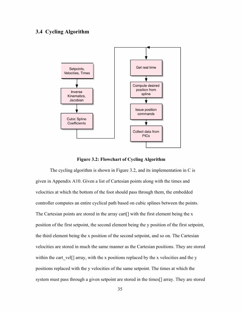
3.4 Cycling Algorithm
Figure 3.2: Flowchart of Cycling Algorithm
The cycling algorithm is shown in Figure 3.2, and its implementation in C is
given in Appendix A10. Given a list of Cartesian points along with the times and
velocities at which the bottom of the foot should pass through them, the embedded
controller computes an entire cyclical path based on cubic splines between the points.
The Cartesian points are stored in the array cart[] with the first element being the x
position of the first setpoint, the second element being the y position of the first setpoint,
the third element being the x position of the second setpoint, and so on. The Cartesian
velocities are stored in much the same manner as the Cartesian positions. They are stored
within the cart_vel[] array, with the x positions replaced by the x velocities and the y
positions replaced with the y velocities of the same setpoint. The times at which the
system must pass through a given setpoint are stored in the times[] array. They are stored

36
such that the time for the first setpoint is the first element of the array, the time for the
second setpoint is the second element, and so on.
In the interest of maintaining fast closed-loop control of the leg, splines are
generated between encoder values for both the hip and knee motors rather than between
points in Cartesian space. This is because if splines were done in Cartesian space, it
would require inverse kinematics and the inverse Jacobian to be computed in real-time.
Since the inverse kinematics equation is stated above as taking 40 milliseconds to
compute, it would simply take too much time to do all the necessary calculations and
maintain fast closed-loop control.
In order that the control may be done effectively in real time, some of the
computations are done beforehand. The computation of the inverse kinematics and the
inverse Jacobian is done first using computeSpline(). The encoder values for the hip are
stored in hip_enc[] while the knee encoder values are stored in knee_enc[]. The first
element of hip_enc[] corresponds with the first Cartesian point, the second element
corresponds to the second Cartesian point, and so on. The rates of change of the hip
encoder are stored in the hip_vel[] array while the rates of change for the knee encoder
are stored in the knee_vel[] array. The first element corresponds to the desired rate of
change through the first setpoint, the second element corresponds to the rate of change
through the second setpoint, and so on. The encoder values and rates of change of
encoder values can then be used as the constraints to compute cubic spline coefficients.
Since the inputs given to computeSpline() are encoder values, the coefficients it generates
correspond to a smooth interpolation in joint space, not necessarily Cartesian space. The
hip encoder spline coefficients are stored in the array hipcoeff[] and the knee encoder

37
spline coefficients are stored in kneecoeff[]. Within these arrays, the first four elements
hold the coefficients connecting the first point to the second, the second group of four
elements hold the coefficients connecting the second point to the third, and so on. The
last group of four holds the coefficients used to connect the last point to the first point.
After all of the coefficients are computed between all setpoints, the system has everything
it needs to begin the real-time control loop.
Immediately before entering the loop, the system begins the high-resolution timer
that is built into the KoreBot system. See Appendix A11 for an explanation of what is
required to have access to the system timer. This timer keeps track of the system time
during the cycling routine and is used as the input to computeSplinePos() to get an
encoder value at a particular time. The timer is also used to determine where in the
cycling path it is and which spline coefficients to use. This is done by referencing the
times associated with each setpoint and modifying the index ‘i’ accordingly. This index is
used to determine which cubic spline coefficients to use for the computeSplinePos()
function. The controller then computes the position for the both the hip and the knee
motors as returned by the computeSplinePos(). A basic check is done to see if the values
are within the acceptable range of hip and knee encoder values to avoid contact with the
hard stops present in the system. If the values are outside the accepted bounds, they are
brought to within the satisfactory range.

38
Once the positions for the hip and knee motors are determined, they are issued as
closed-loop commands using the kmot_AdvancedCmd(). After the hip and knee
commands are issued, the system stores the commanded values into the hip_pos[] and
knee_pos[] arrays, respectively. The times at which these commands are issued are also
stored in the control_time[] array. Immediately following this, the controller begins its
feedback loop using the kmot_AdvancedReadHip() and kmotAdvancedRead() commands
from the three PICs as described in Chapter 2. All feedback data is stored in the same
manner as was done previously with vertical jumping, with the exception that the knee
potentiometer value is now stored in the gs[] [1].
By tracking the system time, the leg progresses smoothly from one interpolating
spline to the next, creating a single smooth, connected path between positions in joint
space. In order to keep the leg along these paths determined by the splines, the KoreBot
repeatedly issues closed loop position commands. Though the time between commands
will depend on the amount of time required to complete the cycling loop, as the code is
shown in Appendix A10 it takes approximately six milliseconds to issue a new command
after the previous one has been issued. Approximately 3.3 ms is required for system
feedback, while the remainder is mostly dedicated to computing new commands and
issuing them to the hip and knee PICs. The KoreMotor microcontrollers then use their
internal PID control to move from one commanded point to another, thereby following
the path determined by the system.
3.5 Results
All foot trajectories for cycling in these trials were created by the arbitrary
selection of the author. The points and velocities were chosen in order to achieve a

39
somewhat fluid and natural motion at a high speed. The set of Cartesian points, velocities
and times used for a successful cycling motion can be found within the cycle() function
in Appendix A10, or they can be seen within Figure 3.3 The generated trajectory using
these points can be seen in Figure 3.3 as well, with the Cartesian setpoints superimposed
on the trajectory as a reference. The entire cycle was designed to take exactly 410
milliseconds to complete, and the leg achieved this average over several cycles. Figure
3.3 shows 61 sequential points for one 410 ms cycle, each of which is computed
approximately 6.7 ms after the one before it. This demonstrates the rate at which the
feedback and command loop is closed during real-time operation.
0.05
0.08
0.11
0.14
0.17
0.2
0.23
-0.040.010.060.110.160.21
X Distance (m)
Y D
ista
nce
(m
)
CommandedSpline
ReferencePoints
Figure 3.3: Generated Cubic Spline From Reference Points
When the above trajectory was commanded to the KoreMotor board repeatedly
within the cycle loop described above, odd oscillatory behavior was noticed on the hip
40
motor. This behavior was noticed as well on the knee motor, but to a much lesser extent.
It was determined that the problem was likely derived from the way in which the
derivative term of the PID controller is computed on the KoreMotor board that resulted in
the erratic behavior. The derivative component on the KoreMotor board is computed as
the difference of the current error and the previous error, where error is defined as the
difference between the actual motor position and the desired motor position. Right before
a new position command is issued, the current error is close to zero because of the
tracking of the PID controller. However, once the new setpoint is issued to the motor
microcontroller, the new error jumps dramatically. Thus, the difference of the two gets a
jump discontinuity at that time, causing a jump in the effect of the derivative term. By
repeatedly issuing new commands, the derivative component repeatedly experiences
jump discontinuities, causing the oscillatory behavior witnessed in early testing. This
behavior is thought to be less noticeable than in the hip motor because the higher gains
and torque possible with the knee motor allow it to fight this oscillatory behavior more
easily.
The problem with the derivative term on the KoreMotor microcontrollers could
not be debugged due to a malfunctioning programmer at the time of testing. In order to
remove this unwanted behavior, new gains had to be found for the hip motor so that the
effects of the derivative term could be reduced. Using the kmot_AdvancedCmd()
function using the CLPIDNOW command as developed by Curran and Huang [5], the hip
motor PID controller was tuned using a proportional gain only. The actual gains can be
seen in Appendix A10, where the CLPIDNOW functionality of kmot_AdvancedCmd() is
used within cycle(). The knee motor PID gains were left unchanged.
41
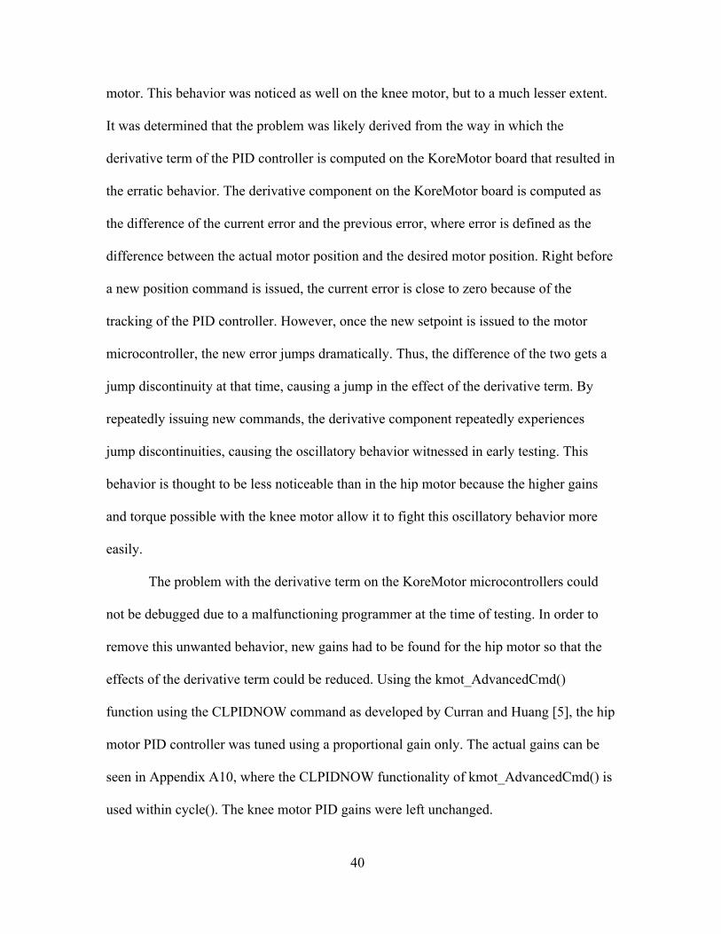
Figure 3.4 shows the resulting trajectory compared to the desired trajectory using
the new gains. The foot does a fairly good job of tracking the desired trajectory, and the
final resulting trajectory is certainly a cyclical motion. A single cycle is completed within
410 milliseconds. This was the fastest the leg was pushed during these preliminary runs,
though several cycles were done at lower speeds. It is able to sustain the rate of 2.5 cycles
per second for an indefinite amount of time terminating only when the system detects a
Control+C interrupt from the keyboard. The leg travels a total distance of approximately
0.55 meters per cycle, with a peak velocity of approximately 3 meters per second across
the bottom of the trajectory. The stroke length along the bottom of the cycling motion is
approximately 16 cm. The cycle has a duty cycle of approximately 30%, meaning that the
foot is pulling along the bottom of its motion for nearly 30% of the entire cycle.
0.05
0.08
0.11
0.14
0.17
0.2
0.23
-0.040.010.060.110.160.21
X Distance (m)
Y D
ista
nce
(m
)
CommandedActual
Figure 3.4: Actual Motion vs. Commanded Motion for One Cycle
42
Based on the trajectory in Figure 3.4, the hip motor is shown to be unable to deal
with the high torque required near the right-hand side of the trajectory. The actual
trajectory goes well beyond the desired trajectory before it can turn around and begin
heading in the positive x-direction. It is here where the acceleration of the hip needs to be
the highest, and the altered gains required to reduce the oscillatory behavior prevents the
hip from being able to follow the desired trajectory exactly. The error in the y-direction is
most likely a result of the hip being unable to follow the desired trajectory in time. The
knee is able to follow its desired trajectory fairly closely in time.
0
1000
2000
3000
4000
5000
6000
7000
8000
9000
10000
0 0.2 0.4 0.6 0.8 1 1.2 1.4
Time (s)
En
cod
er
Valu
e
ActualCommanded
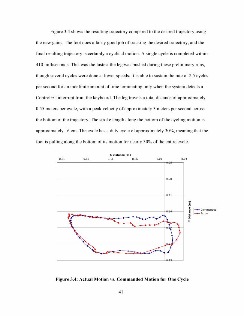
Figure 3.5: Hip Motor Encoder Position vs. Commanded Position for Three Cycles
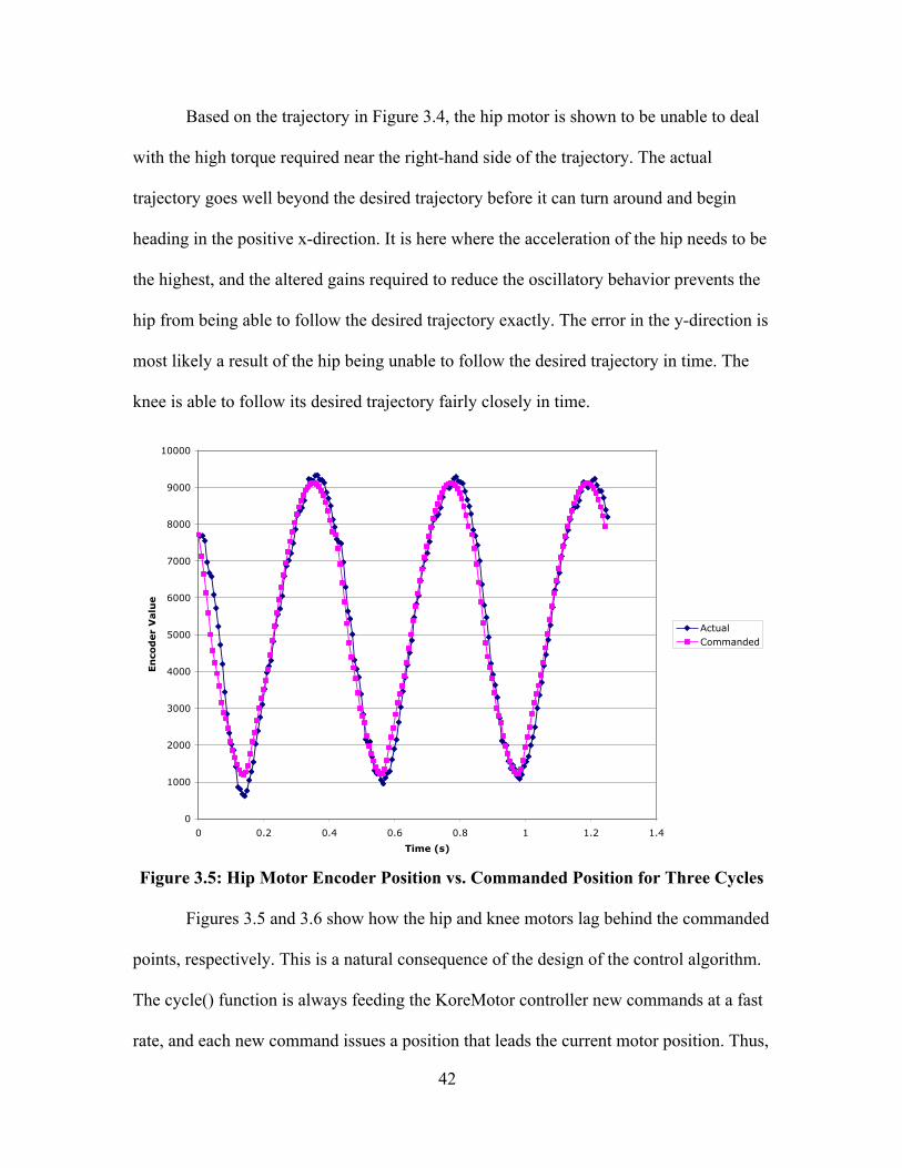
Figures 3.5 and 3.6 show how the hip and knee motors lag behind the commanded
points, respectively. This is a natural consequence of the design of the control algorithm.
The cycle() function is always feeding the KoreMotor controller new commands at a fast
rate, and each new command issues a position that leads the current motor position. Thus,
43
the motors are always trying to keep up with the new commands and consistently lag
behind them as a result. These figures also show how well the knee tracks the
commanded input and how loose the tracking is on the hip. Recall that this is due to the
new PID gains that had to be used for the hip motor in order to avoid the violent
oscillations of the hip motor.
-8000
-6000
-4000
-2000
0
2000
4000
0 0.2 0.4 0.6 0.8 1 1.2 1.4
Time (s)
En
cod
er
valu
e
ActualCommanded
Figure 3.6: Knee Motor Encoder Position vs. Commanded Position for Three Cycles
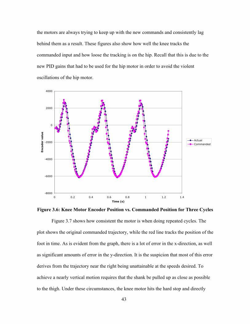
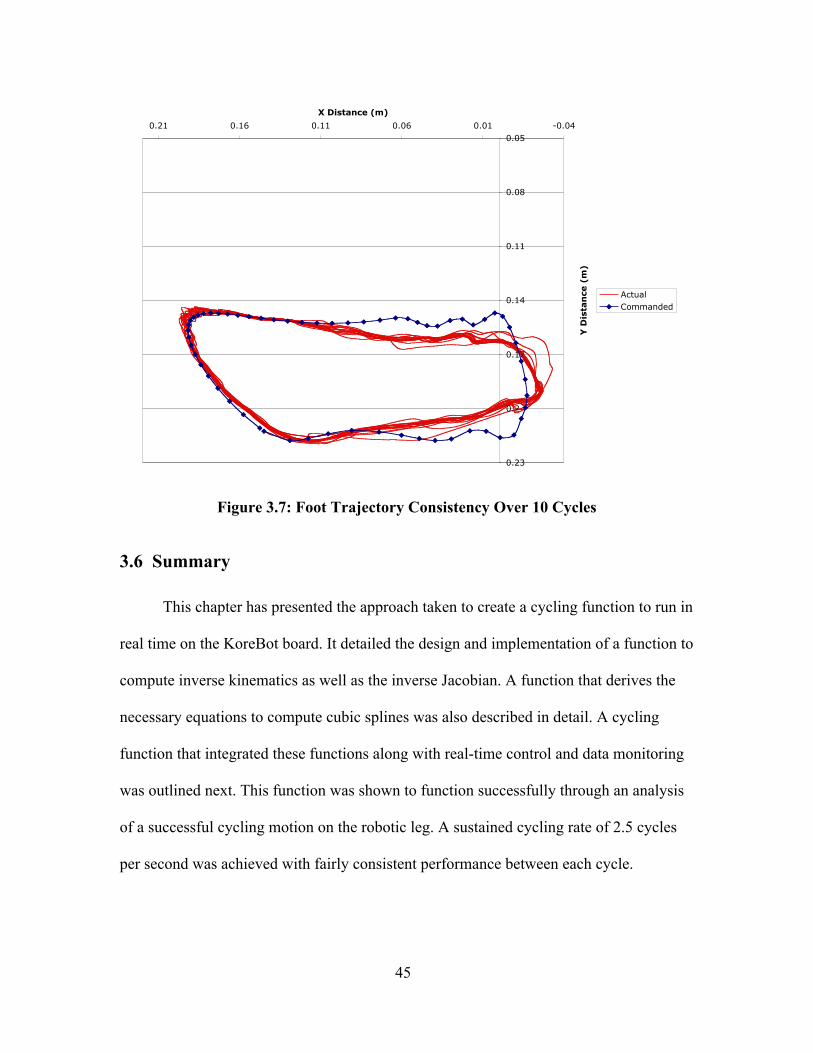
Figure 3.7 shows how consistent the motor is when doing repeated cycles. The
plot shows the original commanded trajectory, while the red line tracks the position of the
foot in time. As is evident from the graph, there is a lot of error in the x-direction, as well
as significant amounts of error in the y-direction. It is the suspicion that most of this error
derives from the trajectory near the right being unattainable at the speeds desired. To
achieve a nearly vertical motion requires that the shank be pulled up as close as possible
to the thigh. Under these circumstances, the knee motor hits the hard stop and directly
44
couples the shank to the thigh. At this point, the knee motor can overcome the hip motor,
pulling it forward. By redesigning the trajectory to be further below the hip axis, some of
these issues could be resolved. The high velocities dictated through these ranges also
make precise control more difficult to achieve. It is also important to note that the first
cycle has noticeably more error than the others. This is due to the fact that the splines
computed for the cycling motion incorporate initial velocities at all points, but when first
beginning a motion the leg does not have any forward motion. Thus, the motors are given
a trajectory that progresses faster through space than they can keep up with initially. The
hip motor, with its lower power output and smaller gains, does worse than the knee motor
(Figure 3.5, 3.6) at tracking initially. Given that the hip has the largest effect on
horizontal position, this explains why the error in the first cycle is particularly bad in the
x-direction as compared to later cycles. With the exception of the first cycle, the foot
position is very consistent through repeated cycles. This indicates that the splines are at
least computed efficiently and correctly throughout the course of the cycling motion. The
ability of the foot position to follow the desired trajectory very closely through the left
half and as reasonably as can be expected through the right half demonstrates that the
proper commands are being generated and transmitted, and more importantly, that tight
control is possible during high-speed cyclical motions.
45
0.05
0.08
0.11
0.14
0.17
0.2
0.23
-0.040.010.060.110.160.21
X Distance (m)
Y D
ista
nce
(m
)
ActualCommanded
Figure 3.7: Foot Trajectory Consistency Over 10 Cycles
3.6 Summary
This chapter has presented the approach taken to create a cycling function to run in
real time on the KoreBot board. It detailed the design and implementation of a function to
compute inverse kinematics as well as the inverse Jacobian. A function that derives the
necessary equations to compute cubic splines was also described in detail. A cycling
function that integrated these functions along with real-time control and data monitoring
was outlined next. This function was shown to function successfully through an analysis
of a successful cycling motion on the robotic leg. A sustained cycling rate of 2.5 cycles
per second was achieved with fairly consistent performance between each cycle.

46
CHAPTER 4
SUMMARY AND CONCLUSIONS
4.1 Summary and Conclusions
As can be seen from Chapters 2 and 3, both high-speed cycling and improved
knee joint sensing and feedback communications were achieved. Successful completion
of these tasks fulfills the research goals of this project as outlined in Chapter 1.
The steps taken to integrate the new potentiometer at the knee joint were unusual
but nevertheless successful. The changes made to the KoreMotor software to process the
analog value allowed it to deal with the new type of input signal while not adding any
noticeable computation time to the previous control software. The changes to the
KoreBot software, when combined with that of the KoreMotor, allowed all feedback
communications to be completed in half the time of the previous system. The ability to
sense the knee angle directly led to interesting data analysis of spring deflections during
vertical jumping as well as the implementation of novel safety routines.
The implementation of cycling was largely successful as well. Despite the setback
with issuing repeated commands that forced the reduction of gains in the PID controller,
the leg was still able to follow the commanded trajectories. It was hypothesized that most
of the tracking error was a result of these reduced gains on the hip motor. The inverse
kinematics and inverse Jacobian computations produced the correct positioning of the
robotic leg, and the cubic spline functions interpolated well between these points. High-
speed cycling was achieved, and the goal of creating a dynamic cyclical motion with the
leg was fulfilled.

47
4.2 Future Work
There are several tasks that can be done in the future to follow up with this
work. The first task is to reduce the noise present on the knee potentiometer signal line.
This must be done in order to allow for accurate control of the shank through knee angle
joint feedback itself rather than through the knee motor. Reducing the noise would also
allow for the accurate calculation of the knee angle velocity, which could in turn lead
towards power analysis of the series-elastic actuator. If the torque can be computed at the
knee, then the power output of the knee could be determined. This would be very helpful
in optimizing the jumping behavior of the leg by optimizing the power output at the knee
joint.
Extending the sensing range of the knee potentiometer could allow for more
complete understanding of the knee and spring through all possible ranges of motion. The
current range of sensing has a region of approximately 5° near the full extension of the
knee in which the potentiometer outputs 0V throughout. By changing the biasing of the
potentiometer, it would be possible to extend the range of the potentiometer to sense
nonzero values near singularity while not losing sensing at the other end of the range of
motion of the shank near the thigh. By having nonzero values near full extension, the
spring deflection value can be more accurately understood through the entire range of
motion of the knee during a jump, as well as any future utilizations of the series-elastic
actuation. Also, work on development of an accurate relationship between the
potentiometer value and knee angle should be explored (Appendix 6).
The creation of a MATLAB script could be generated to allow for easier
generation of foot trajectories during cycling. The current method of developing

48
trajectories involves picking rough values of position and velocity and then optimizing
manually. The script could generate smooth trajectories in Cartesian space and then
translate them to a set of positions, velocities, and times that could be used as direct
inputs to the cycle command. Within this script, it would also be possible to check each
commanded point to make sure that it is within the workspace of the leg. This could be
used to avoid the problem in which the shank hits the hard stop on the thigh, forcing the
foot to follow undesired trajectories.
A better solution to creating smooth Cartesian trajectories would be to have the
inverse kinematics and inverse Jacobian run in real time. The cubic splines could be
generated in Cartesian space and could generate Cartesian position commands in real
time, allowing for much more smooth trajectories. However, because the inverse
kinematics and inverse Jacobian take so long currently to compute, it is impractical to do
these calculations in real time. Fortunately, efforts are currently underway to reduce this
computation time, but there is still work to be done to this end.
It would also be useful if, within the cycling function, there could be a way to
scale the speed of the cycling smoothly through some sort of user input. Currently, in
order to change the speed of the cycling, the times and velocities must both be adjusted.
If there were a type of normalization factor that could be controlled by the user, this
would allow for quick and easy alterations of the cycling speed.
Even using the current method of spline generation, it would be interesting to
have the leg cycle and bring the leg into contact with the ground near the bottom of the
stroke. The dynamics of the system would change dramatically from the tests shown in
this report. This could produce interesting results and open new paths for future research.

49
This cycling with ground contact could also take advantage of the ability to compute
spring deflection during the cycling motion, as well.
The utilization of the KoreIO board could offload some computational demands
from the KoreMotor board. It could be used to take in the analog input from the knee
potentiometer as well as other inputs that may be added to the system in the future.
Currently, the KoreIO board is using the original K-Team I2C protocol and cannot be
reprogrammed because that code is unavailable. Until it becomes easy to reprogram and
can be used more effectively than the solutions offered in this thesis, the KoreIO’s
computational power will be neglected.
The current proportional-derivative (PD) controller used in the cycling motions
needs to be fixed in order to allow for repeated position commands to be issued while
retaining a large derivative gain. As discussed in Section 3.5, the erratic oscillatory
behavior that arose from the use of the derivative term of the PD control forced the entire
derivative term to be removed. If the way in which the derivative term is computed can
be corrected, it would allow the derivative term to be used again in the PD control for
cycling. This would allow for faster responses and more precise motion control.
There is much work that can be done based on the research presented in this
document. Hopefully the efforts made thus far can contribute to the continued growth of
understanding of the series-elastic actuated robotic leg in high-speed dynamic motions.
These insights might then be applied to the design of future series-elastic systems under
the guidance of Dr. Orin and Dr. Schmiedeler.

50
Appendix A1: Values for Physical Parameters of Leg
Table A1.1: Physical Leg
Parameters [1]
Figure A1.1: Physical Representation of Leg [1]
Parameter Length (cm)
lt 14.0
ls 12.7
lh 10.8
rf 1.90
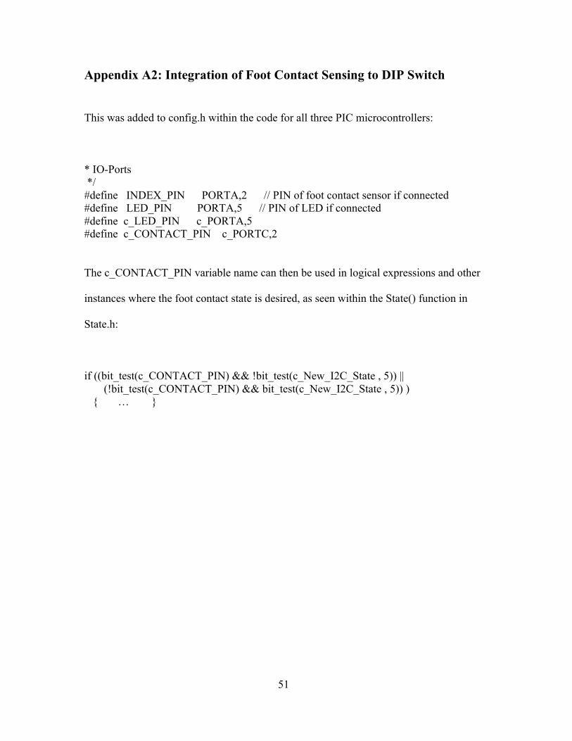
51
Appendix A2: Integration of Foot Contact Sensing to DIP Switch
This was added to config.h within the code for all three PIC microcontrollers:
* IO-Ports */#define INDEX_PIN PORTA,2 // PIN of foot contact sensor if connected#define LED_PIN PORTA,5 // PIN of LED if connected#define c_LED_PIN c_PORTA,5#define c_CONTACT_PIN c_PORTC,2
The c_CONTACT_PIN variable name can then be used in logical expressions and other
instances where the foot contact state is desired, as seen within the State() function in
State.h:
if ((bit_test(c_CONTACT_PIN) && !bit_test(c_New_I2C_State , 5)) || (!bit_test(c_CONTACT_PIN) && bit_test(c_New_I2C_State , 5)) ) { … }

52
Appendix A3: Integration of Analog-to-Digital Conversion on theKoreMotor Board
In order to properly initialize the ADC unit on the PIC18F4431, the CCS compiler
requires that the proper arguments be given to the setup_adc_ports() and
set_adc_channel() functions. This is done within controler.c:
… #ifdef PIC18F4431 /* AN0:AN1 are Analog inputs, VREF+ = VDD, VREF- = VSS */ setup_adc_ports(sAN0|sAN1|sAN2|VSS_VDD); set_adc_channel(2); //Added sAN2 for index pin, ADC_CONT_C, set_adc_channel 11/30/2006
…
An analog-to-digital conversion begins at the start of a feedback cycle within controler.c:
…//==============================================================// S T A R T A N E W C Y C L E//==============================================================NewCycle: /* 07/24/2006 Add State_Change() for detecting foot contact and change state */
read_adc(ADC_START_ONLY);
State_Change();…
The digital value that results from the conversion is then later read within measure.h:
…void Measure(){/* update position specific to the Encoder * position is stored in <PositionNew> on Bank 1 */ SpecEncPos();
c_ADC_value = read_adc(ADC_READ_ONLY);…

53
Appendix A4: New I2C Feedback Protocol
The new I2C feedback protocol for the hip PIC only is shown below. It is located in thei2c.h header file within the hip PIC directory.
/*--------------------------------------------------------------------*/char new_i2c_prepare_data (){ char ch; //Declare a variable for storing the returned value
#asm clrf BSR //Set RAM to bank 0 which i2c accessible #endasm
//Determine which data byte has been returned using I2C Data Index reg. switch(c_I2C_DATA_INDEX) {
case 0xFF: //Data byte 1 c_Position32 = c_PositionNew32; //Update 32 bits Position reg.
c_Speed16 = c_SpeedCopy; //Update 16 bits speed value c_PosH = c_PositionHL; //Divide position and speed reg. into 8bits each c_PosM = c_PositionLH; c_PosL = c_PositionLL;
ch = c_PosH; //Return higher byte of position value c_I2C_DATA_INDEX --; //Point to next data byte to return break;
case 0xFE: //Data byte 2 ch = c_PosM; //Return middle byte of position value c_I2C_DATA_INDEX --; //Point to next byte of data to return break;
case 0xFD: //Data byte 3 ch = c_PosL; //Return lower byte od position value c_I2C_DATA_INDEX --; //Point to next byte of data to return break;
case 0xFC:
c_SpeH = c_SpeedH; c_SpeL = c_SpeedL;
ch = c_SpeH; //Data byte 4 if (bit_test(c_CONTACT_PIN)) //Return the higher byte od speed value bit_clear(ch , 7); //The MSB indicates the state of Index pin else bit_set(ch , 7);
c_I2C_DATA_INDEX --; break;

54
case 0xFB: //Data byte 5 ch = c_SpeL; //Return lower byte of speed value c_I2C_DATA_INDEX --; break;
case 0xFA: ch = c_ADC_valueH; c_I2C_DATA_INDEX --; break;
case 0xF9: ch = c_ADC_valueL; c_I2C_DATA_INDEX = 0x00; //Set index reg. to initial for receiving new command bit_clear(c_New_I2c_State , 6); //Disable new I2C read mode bit_clear(c_New_I2c_State , 7); //Disable new I2C communication protocol i2c_state = 0; //Initialize the i2c state break;
default: //Prevent error i2c read operation c_I2C_DATA_INDEX = 0x00; bit_clear(c_New_I2c_State , 6); bit_clear(c_New_I2c_State , 7); i2c_state = 0; break;
}
return ch; //Return value back to main i2c interrupt subroutine}/*--------------------------------------------------------------------*/

55
Appendix A5: New kmot_AdvancedReadHip Function
The new kmot_AdvancedReadHip function is first declared within kmot.h:
extern void kmot_AdvancedReadHip( knet_dev_t * dev, int * position, int * speed, int * state, int* knee);
The function itself is defined in kmot.c:
void kmot_AdvancedReadHip( knet_dev_t * dev, int * position, int * speed, int * state, int * knee) //HipRead guess{unsigned char *tmp_pos = (unsigned char *)position;unsigned char *tmp_speed = (unsigned char *)speed;void kmot_AdvancedReadHip( knet_dev_t * dev, int * position, int * speed, int * state, int * knee) //HipRead guess{unsigned char *tmp_pos = (unsigned char *)position;unsigned char *tmp_speed = (unsigned char *)speed;unsigned char *tmp_state = (unsigned char *)state;unsigned char *tmp_knee = (unsigned char *)knee;unsigned char reg = (unsigned char)0x28;unsigned char cmd = (unsigned char)0x8D;unsigned char return_buf[10];int rc;
rc = knet_readNew(dev, reg, cmd, &return_buf[0], 7); // Return 7?tmp_pos[0] = return_buf[2];tmp_pos[1] = return_buf[1];tmp_pos[2] = return_buf[0];
//bit extend reg 0x36if((tmp_pos[2] & (unsigned char)0x80) > 0){ tmp_pos[3] = (unsigned char)0xFF;}else{ tmp_pos[3] = (unsigned char)0x00;}
tmp_state[0] = return_buf[3];if ((tmp_state[0] & (unsigned char)0x80) > 0){tmp_state[0] = (unsigned char)0x01;}else{tmp_state[0] = (unsigned char)0x00;}tmp_state[1] = (unsigned char)0x00;tmp_state[2] = (unsigned char)0x00;tmp_state[3] = (unsigned char)0x00;
tmp_speed[1] = return_buf[3] & (unsigned char)0x7F;

56
if((tmp_speed[1] & (unsigned char)0x40) > 0){ tmp_speed[1] = tmp_speed[1]|(unsigned char)0x80; tmp_speed[2] = (unsigned char)0xFF; tmp_speed[3] = (unsigned char)0xFF;}else{ tmp_speed[2] = (unsigned char)0x00; tmp_speed[3] = (unsigned char)0x00;}
tmp_speed[0] = return_buf[4];
tmp_knee[1] = return_buf[5];tmp_knee [0] = return_buf[6];tmp_knee[2] = 0x00;tmp_knee[3] = 0x00;}
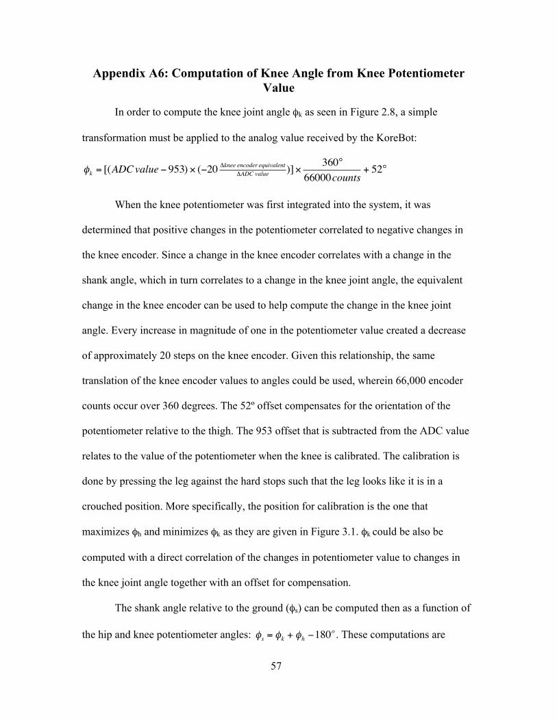
57
Appendix A6: Computation of Knee Angle from Knee PotentiometerValue
In order to compute the knee joint angle φk as seen in Figure 2.8, a simple
transformation must be applied to the analog value received by the KoreBot:
€
φk = [(ADCvalue − 953) × (−20 Δknee encoder equivalentΔADC value )]× 360°
66000counts+ 52°
When the knee potentiometer was first integrated into the system, it was
determined that positive changes in the potentiometer correlated to negative changes in
the knee encoder. Since a change in the knee encoder correlates with a change in the
shank angle, which in turn correlates to a change in the knee joint angle, the equivalent
change in the knee encoder can be used to help compute the change in the knee joint
angle. Every increase in magnitude of one in the potentiometer value created a decrease
of approximately 20 steps on the knee encoder. Given this relationship, the same
translation of the knee encoder values to angles could be used, wherein 66,000 encoder
counts occur over 360 degrees. The 52º offset compensates for the orientation of the
potentiometer relative to the thigh. The 953 offset that is subtracted from the ADC value
relates to the value of the potentiometer when the knee is calibrated. The calibration is
done by pressing the leg against the hard stops such that the leg looks like it is in a
crouched position. More specifically, the position for calibration is the one that
maximizes φh and minimizes φk as they are given in Figure 3.1. φk could be also be
computed with a direct correlation of the changes in potentiometer value to changes in
the knee joint angle together with an offset for compensation.
The shank angle relative to the ground (φs) can be computed then as a function of
the hip and knee potentiometer angles:
€
φs = φk + φh −180o . These computations are

58
accurate when the shank is within +/- 60 degrees from the vertical. Beyond these ranges,
the approximation relating the knee potentiometer value does not hold as well and the
computations don’t hold as well. A more accurate calculation of the relationship between
the changes in potentiometer value and changes in the equivalent knee encoder value
might ameliorate the erroneous calculations near the edge of the range of motion of the
knee. There is no significant reason to refrain from using a float value instead of the
integer approximation in that calculation.

59
Appendix A7: Safety Routines Added to the KoreMotor Board
The following functions were modified within control.h. The changes revolve around the
conditional statements that determine if the system is allowed to either give the closed
loop command (PreparePos) or enter into open loop control (OpenLoop):
void PreparePos(){ //if(bit_test(c_SOFTSTOP_FLAG) && c_PositionOld32 < c_SoftStopMin) if(bit_test(c_SOFTSTOP_FLAG) && c_SetPointCopy < c_SoftStopMin) //----- c_SetPointCopy = c_SoftStopMin; // | 01/06/2007 // if(bit_test(c_SOFTSTOP_FLAG) && c_PositionOld32 > c_SoftStopMax)// | Added for smart leg inPID position limit if(bit_test(c_SOFTSTOP_FLAG) && c_SetPointCopy > c_SoftStopMax) //------ c_SetPointCopy = c_SoftStopMax;
c_Process = c_PositionOld32;
c_Kp = c_KpPos; c_Kd = c_KdPos; c_Ki = c_KiPos;
return;}
//================// Open-Loop-Mode//================
void OpenLoop(){ /* Bypass the controller * Limit the setpoint value to 9bit * only. Sign is stored in bit 15 */ if(!bit_test(c_CONTACT_PIN) && c_ADC_value < 50 && bit_test(c_KNEE_SAFETY_FLAG)) { c_SetPoint = 0; c_SetPointCopy = 0; c_PID_OUT16 = 0; bit_set(c_NEW_SETPOINT_FLAG); bit_set(c_LED_PIN); //Debugging purposes return; }
if(abs(c_SetPoint) >= 0x1FF) c_PID_OUT16 = 0x01FF; else c_PID_OUT16 = abs(c_SetPoint);

60
if(bit_test(c_SetPoint,31)) bit_set(c_PID_OUT16,15); else bit_clear(c_PID_OUT16,15);
bit_clear(c_LED_PIN); return;}
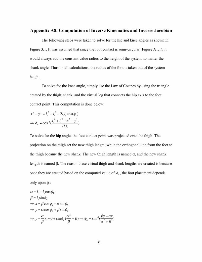
61
Appendix A8: Computation of Inverse Kinematics and Inverse Jacobian
The following steps were taken to solve for the hip and knee angles as shown in
Figure 3.1. It was assumed that since the foot contact is semi-circular (Figure A1.1), it
would always add the constant value radius to the height of the system no matter the
shank angle. Thus, in all calculations, the radius of the foot is taken out of the system
height.
To solve for the knee angle, simply use the Law of Cosines by using the triangle
created by the thigh, shank, and the virtual leg that connects the hip axis to the foot
contact point. This computation is done below:
€
x 2 + y 2 = ls2 + lt
2 − 2lslt cos(φk )
⇒φk = cos−1( ls2 + lt
2 − x 2 − y 2
2lslt)
To solve for the hip angle, the foot contact point was projected onto the thigh. The
projection on the thigh set the new thigh length, while the orthogonal line from the foot to
the thigh became the new shank. The new thigh length is named α, and the new shank
length is named β. The reason these virtual thigh and shank lengths are created is because
once they are created based on the computed value of
€
φk , the foot placement depends
only upon φh:
€
α = lt − ls cosφkβ = ls sinφk⇒ x = β cosφh −α sinφh⇒ y =α cosφh + β sinφh
⇒ y − αβx = 0 + sinφh (
α 2
β+ β)⇒φh = sin−1(βy −αx
α 2 + β 2)
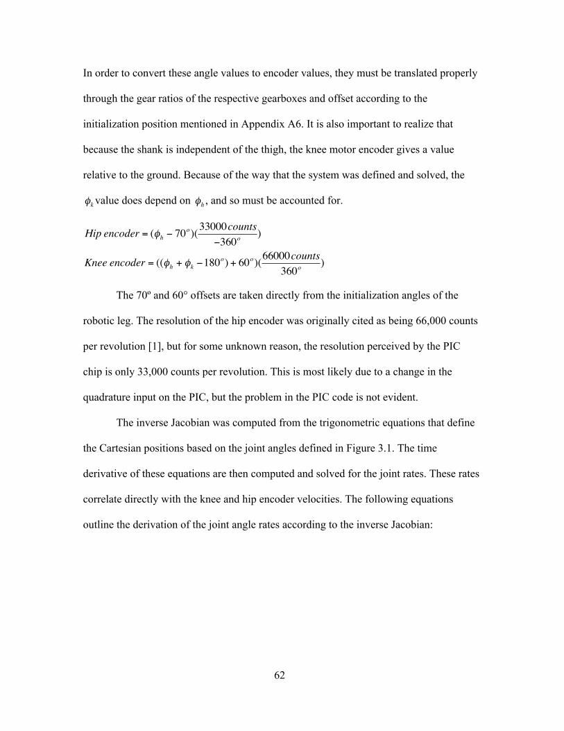
62
In order to convert these angle values to encoder values, they must be translated properly
through the gear ratios of the respective gearboxes and offset according to the
initialization position mentioned in Appendix A6. It is also important to realize that
because the shank is independent of the thigh, the knee motor encoder gives a value
relative to the ground. Because of the way that the system was defined and solved, the
€
φkvalue does depend on
€
φh , and so must be accounted for.
€
Hip encoder = (φh − 70o)(33000counts
−360o)
Knee encoder = ((φh + φk −180o) + 60o)(66000counts
360o)
The 70º and 60° offsets are taken directly from the initialization angles of the
robotic leg. The resolution of the hip encoder was originally cited as being 66,000 counts
per revolution [1], but for some unknown reason, the resolution perceived by the PIC
chip is only 33,000 counts per revolution. This is most likely due to a change in the
quadrature input on the PIC, but the problem in the PIC code is not evident.
The inverse Jacobian was computed from the trigonometric equations that define
the Cartesian positions based on the joint angles defined in Figure 3.1. The time
derivative of these equations are then computed and solved for the joint rates. These rates
correlate directly with the knee and hip encoder velocities. The following equations
outline the derivation of the joint angle rates according to the inverse Jacobian:

63
€
x = −lt sin(φh ) + ls sin(180°−φh −φk )y = lt cos(φh ) + ls cos(180°−φh −φk ) + .01905mdxdt
= −lt cos(φh )dφhdt
+ ls cos(180°−φh −φk ) × (−dφhdt
+−dφkdt
)
dydt
= −lt sin(φh )dφhdt
− ls sin(180°−φh −φk ) × (−dφhdt
+−dφkdt
)
φh, φh ,dxdt, dydt, ls, and lt are known
From the dxdtequation :
dφkdt
=
dxdt
+ ltdφhdtcos(φh ) + ls
dφhdtcos(180°−φh −φk )
−ls cos(180°−φh −φk )
Substituting in dydtequation :
dφhdt[−lt sin(φh ) + ls sin(180°−φh −φk ) +
lslt sin(180°−φh −φk )cos(φh )ls cos(180°−φh −φk )
+ ls sin(180°−φh −φk )]
=dydt
+lsdxdtsin(180°−φh −φk )
ls sin(180°−φh −φk )Solving :
dφhdt
=
dydt
+ ls(dxdt)sin(180°−φh −φk )
−lt sin(φh ) − ls sin(180°−φh −φk ) − lt tan(180°−φh −φk )cos(φh ) + ls sin(180°−φh −φk )
dφkdt
=[− dxdt− lt cos(φh )
dφhdt]
−ls cos(180°−φh −φk )−dφhdt
The following function is the C implementation of this mathematical derivation
within in hopper.c that is used within the KoreBot to compute the inverse kinematics and
the inverse Jacobian:
int inversek( float x, float y, float xprime, float yprime, int *kneeptr, int *hipptr, float *kvelptr, float*hvelptr ){
float r = 0.01905; float ls = 0.12065; float lt = 0.1397; float t_2p = 0.0; float t_2n = 0.0;
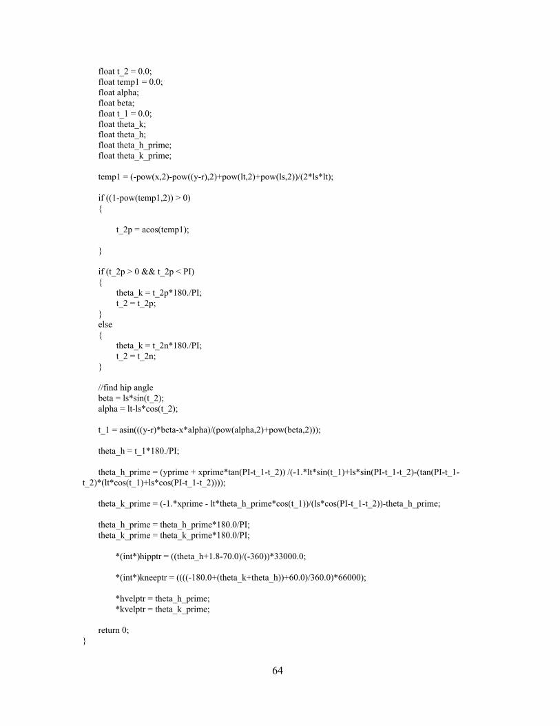
64
float t_2 = 0.0; float temp1 = 0.0; float alpha; float beta; float t_1 = 0.0; float theta_k; float theta_h; float theta_h_prime; float theta_k_prime;
temp1 = (-pow(x,2)-pow((y-r),2)+pow(lt,2)+pow(ls,2))/(2*ls*lt);
if ((1-pow(temp1,2)) > 0) {
t_2p = acos(temp1);
}
if (t_2p > 0 && t_2p < PI) { theta_k = t_2p*180./PI; t_2 = t_2p; } else { theta_k = t_2n*180./PI; t_2 = t_2n; }
//find hip angle beta = ls*sin(t_2); alpha = lt-ls*cos(t_2);
t_1 = asin(((y-r)*beta-x*alpha)/(pow(alpha,2)+pow(beta,2)));
theta_h = t_1*180./PI;
theta_h_prime = (yprime + xprime*tan(PI-t_1-t_2)) /(-1.*lt*sin(t_1)+ls*sin(PI-t_1-t_2)-(tan(PI-t_1-t_2)*(lt*cos(t_1)+ls*cos(PI-t_1-t_2))));
theta_k_prime = (-1.*xprime - lt*theta_h_prime*cos(t_1))/(ls*cos(PI-t_1-t_2))-theta_h_prime;
theta_h_prime = theta_h_prime*180.0/PI; theta_k_prime = theta_k_prime*180.0/PI;
*(int*)hipptr = ((theta_h+1.8-70.0)/(-360))*33000.0;
*(int*)kneeptr = ((((-180.0+(theta_k+theta_h))+60.0)/360.0)*66000);
*hvelptr = theta_h_prime;*kvelptr = theta_k_prime;
return 0;}
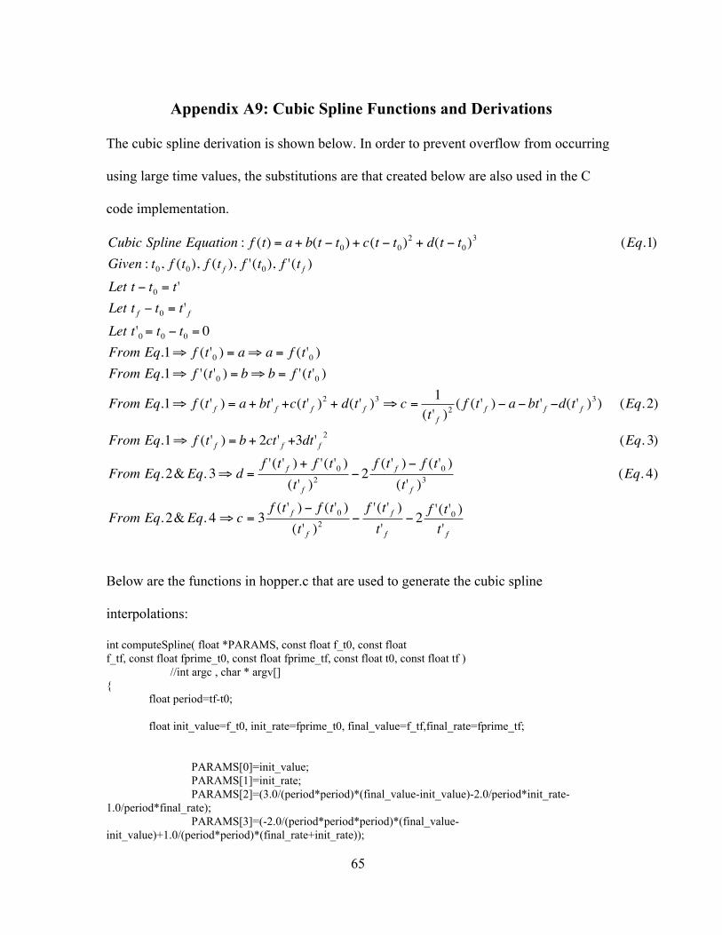
65
Appendix A9: Cubic Spline Functions and Derivations
The cubic spline derivation is shown below. In order to prevent overflow from occurring
using large time values, the substitutions are that created below are also used in the C
code implementation.
€
Cubic Spline Equation : f (t) = a + b(t − t0) + c(t − t0)2 + d(t − t0)
3 (Eq.1)Given : t0, f (t0), f (t f ), f '(t0), f '(t f )Let t − t0 = t 'Let t f − t0 = t' fLet t '0 = t0 − t0 = 0From Eq.1⇒ f (t '0 ) = a⇒ a = f (t'0 )From Eq.1⇒ f '(t '0 ) = b⇒ b = f '(t'0 )
From Eq.1⇒ f (t ' f ) = a + bt' f +c(t' f )2 + d(t ' f )
3 ⇒ c =1
(t ' f )2 ( f (t ' f ) − a − bt' f −d(t' f )
3) (Eq. 2)
From Eq.1⇒ f (t ' f ) = b + 2ct' f +3dt ' f2 (Eq. 3)
From Eq. 2&Eq. 3⇒ d =f '(t ' f ) + f '(t'0 )
(t' f )2 − 2
f (t ' f ) − f (t'0 )(t' f )
3 (Eq. 4)
From Eq. 2&Eq. 4⇒ c = 3f (t ' f ) − f (t'0 )
(t' f )2 −
f '(t ' f )t' f
− 2 f '(t'0 )t ' f
Below are the functions in hopper.c that are used to generate the cubic spline
interpolations:
int computeSpline( float *PARAMS, const float f_t0, const floatf_tf, const float fprime_t0, const float fprime_tf, const float t0, const float tf ) //int argc , char * argv[]{
float period=tf-t0;
float init_value=f_t0, init_rate=fprime_t0, final_value=f_tf,final_rate=fprime_tf;
PARAMS[0]=init_value;PARAMS[1]=init_rate;PARAMS[2]=(3.0/(period*period)*(final_value-init_value)-2.0/period*init_rate-
1.0/period*final_rate);PARAMS[3]=(-2.0/(period*period*period)*(final_value-
init_value)+1.0/(period*period)*(final_rate+init_rate));
66
return 0;}
int computeSplinePos(const double t, float *PARAMS){ //Returns f(t) for a spline with PARAMS. double t2=t*t, t3=t2*t; return PARAMS[0]+PARAMS[1]*t+PARAMS[2]*t2+PARAMS[3]*t3;}

67
Appendix A10: Cycle Function
Below is the function created within hopper.c to control the real-time cycling:
int cycle( int argc , char *argv[] ){// This function needs the first two arguments to be the starting point// in Cartesian coordinates in meters.// From there on, it takes arguments in groups of three,// where each group corresponds to a different point on the trajectory.// In each group of three, the arguments should be in the following format:// First argument - X coordinate, in meters// Second argument - Y coordinate, in meters// Third argument - time, in microseconds
FILE *archive;FILE *outfile1;FILE *outfile2;FILE *h_p;FILE *h_s;FILE *k_p;FILE *k_s;FILE *g_p;FILE *g_s;FILE *p_p;FILE *p_s;FILE *c_h;FILE *c_k;
float pot_offset = -2.1;
int elapsed_time = 0;int setpoints = 8; //number of splines through which it must travelint i = 1; //index for state between setpointsfloat cart_vel[2*setpoints];int knee_enc[setpoints+1]; //stores the encoder values for the setpointsint hip_enc[setpoints+1]; //stores the encoder values for the setpointsfloat hip_vel[setpoints+1];float knee_vel[setpoints+1];int times[setpoints+1]; //stores the times for the setpointsfloat kneecoeff[setpoints*4]; //stores the coefficients for the splinesfloat hipcoeff[setpoints*4]; //stores the coefficients for the splinesfloat cart[setpoints*2];int current_knee; //holds current position as computed by the splineint current_hip; //holds current position as computed by the splineint counter = 1; //stores running tally of number of data pointsint knee_pos[10000]; //stores the commanded encoder valuesint hip_pos[10000]; //stores the commanded encoder valuesint control_time[10000]; //stores the time at which commanded values were computedint total_usecs = 0; //holds the timechar *junk;char buf2[32];
68
char directory_string[200];char junk2[200];char set_name[50];int test_number = 0;
int hp[10000];int hs[10000];int ch[10000];int h_t[10000];int kp[10000];int ks[10000];int ck[10000];int k_t[10000];int gp[10000];int gs[10000];int g_t[10000];int pp[10000];int ps[10000];int p_t[10000];
int data[4] = {0,0,0,0};
times[0] = 0;times[1] = 35000;times[2] = 70000;times[3] = 92000;times[4] = 102000;times[5] = 147000;times[5] = 160000;times[6] = 179000;times[7] = 215000;times[8] = 410000;
cart[0] = 0.145;cart[1] = 0.21;//horizontalcart[2] = .08;cart[3] = .21;//horizontalcart[4] = 0.02;cart[5] = 0.21;//horizontalcart[6] = -.01;cart[7] = 0.21;//horizontalcart[8] = -.015;cart[9] = 0.198;//maybe start moving upcart[10] = 0.01;cart[11] = .15;cart[12] = 0.03;cart[13] = 0.15;//move up and leftcart[14] = 0.06681;cart[15] = 0.15;//move left and down a bitcart[16] = 0.10;cart[17] = 0.153;//down and left slightlycart_vel[0] = .3/3.;cart_vel[1] = 0.;cart_vel[2] = 0.7/3.;cart_vel[3] = 0.;

69
cart_vel[4] = 0.7/3.;cart_vel[5] = 0.0;cart_vel[6] = 0.7/3.;cart_vel[7] = 0.0;cart_vel[8] = .1;cart_vel[9] = 0.4; //changed to negativecart_vel[10] = -0.4/3.;cart_vel[11] = -.3/.3;cart_vel[12] = -0.4/3.;cart_vel[13] = -0.3/3.;cart_vel[14] = -0.4/3.;cart_vel[15] = -0.3/3.;cart_vel[16] = -0.3/3.;cart_vel[17] = -0.5/3.;
/*
*/
//Open file pointersif ( (outfile1 = fopen( "/home/hopper/hip_enc.dat","w")) == NULL)
{printf("Can't open %s\n","hip_enc.dat");stopReq=1;}
if ( (outfile2 = fopen( "/home/hopper/knee_enc.dat","w")) == NULL){
printf("Can't open %s\n","knee_enc.dat");stopReq=1;
}if ( (h_p = fopen( "/home/hopper/hip_pos.dat","w")) == NULL){
printf("Can't open %s\n","hip_pos.dat");stopReq=1;
}if ( (h_s = fopen( "/home/hopper/hip_speed.dat","w")) == NULL){
printf("Can't open %s\n","hip_speed.dat");stopReq=1;
}if ( (k_p = fopen( "/home/hopper/knee_pos.dat","w")) == NULL){
printf("Can't open %s\n","knee_pos.dat");stopReq=1;
}if ( (k_s = fopen( "/home/hopper/knee_speed.dat","w")) == NULL){
printf("Can't open %s\n","knee_speed.dat");stopReq=1;
}if ( (g_p = fopen( "/home/hopper/gurley_pos.dat","w")) == NULL){
printf("Can't open %s\n","gurley_pos.dat");stopReq=1;
}if ( (g_s = fopen( "/home/hopper/gurley_speed.dat","w")) == NULL)

70
{printf("Can't open %s\n","gurley_speed.dat");stopReq=1;
}if ( (c_h = fopen( "/home/hopper/foot_contactHip.dat","w")) == NULL){
printf("Can't open %s\n","foot_contactHip.dat");stopReq=1;
}if ( (c_k = fopen( "/home/hopper/foot_contactKnee.dat","w")) == NULL){
printf("Can't open %s\n","foot_contactKnee.dat");stopReq=1;
}
//Retrieve location for data storagesystem ("cp /mnt/nfs/v7/data_archive/Cycling/Archive_Cycle.dat /home/hopper/");archive = fopen( "/home/hopper/Archive_Cycle.dat", "r");get_cycledir(archive, set_name, &test_number, directory_string);fclose(archive);printf("Data will be stored in directory: %s\n", directory_string);archive = fopen( "/home/hopper/Archive_Cycle.dat", "w");increment_archive_file(archive, set_name, test_number);fclose(archive);system ("cp /home/hopper/Archive_Cycle.dat /mnt/nfs/v7/data_archive/Cycling/");
//Compute inverse kinematics to get the initial foot position// inversek(atof(argv[1]),atof(argv[2]), 0, 0, &knee_enc[0], &hip_enc[0], &knee_vel[0],&hip_vel[0]);// knee_pos[0] = knee_enc[0];// hip_pos[0] = hip_enc[0];// control_time[0] = 0;// times[0]=0;
inversek(cart[0],cart[1], cart_vel[0], cart_vel[1], &knee_enc[0], &hip_enc[0], &knee_vel[0],&hip_vel[0]);
knee_pos[0] = knee_enc[0];hip_pos[0] = hip_enc[0];control_time[0] = 0;
//Compute the inverse kinematics for remaining points and compute the spline coefficientswhile((i<setpoints) && !stopReq) //do all intense computations first{
// printf("arguments %i\t%f\t%f\n",atoi(argv[((i-1)*3)]),atof(argv[3*(i-1)+1]),atof(argv[3*(i-1)+2]) );// times[i] = (atoi(argv[((i-1)*3)+5]));
// printf("times[%i] = %i\n", (i), times[i]);// inversek(atof(argv[3*(i-1)+3]),atof(argv[3*(i-1)+4]), 0, 0, &knee_enc[i], &hip_enc[i],&knee_vel[i], &hip_vel[i]);// printf("%i\t%i\n",knee[i],hip[i]);// computeSpline(&kneecoeff[4*(i-1)], knee_enc[i-1], knee_enc[i], knee_vel[i-1],knee_vel[i], times[i-1]/1000., times[i]/1000.); //&kneecoeff
71
// computeSpline(&hipcoeff[4*(i-1)], hip_enc[i-1], hip_enc[i], hip_vel[i-1], hip_vel[i],times[i-1]/1000., times[i]/1000. );
inversek(cart[2*i],cart[2*i+1], cart_vel[2*i], cart_vel[2*1+1] , &knee_enc[i],&hip_enc[i], &knee_vel[i], &hip_vel[i]);
computeSpline(&kneecoeff[4*(i-1)], knee_enc[i-1], knee_enc[i], knee_vel[i-1],knee_vel[i], times[i-1]/1000., times[i]/1000.); //&kneecoeff
computeSpline(&hipcoeff[4*(i-1)], hip_enc[i-1], hip_enc[i], hip_vel[i-1], hip_vel[i],times[i-1]/1000., times[i]/1000. );
i += 1;}
inversek(cart[2*i],cart[2*i+1], cart_vel[2*i], cart_vel[2*i+1], &knee_enc[i], &hip_enc[i],&knee_vel[i], &hip_vel[i]);
computeSpline(&kneecoeff[4*(i-1)], knee_enc[i-1], knee_enc[0], knee_vel[i-1], knee_vel[0],times[i-1]/1000., times[i]/1000.);
computeSpline(&hipcoeff[4*(i-1)], hip_enc[i-1], hip_enc[0], hip_vel[i-1], hip_vel[0], times[i-1]/1000., times[i]/1000. );
// printf("Knee coefficients:\n");//
printf("%f\t%f\t%f\t%f\n",kneecoeff[4*(1)],kneecoeff[4*(1)+1],kneecoeff[4*(1)+2],kneecoeff[4+3]);// printf("Hip coefficients:\n");// printf("%f\t%f\t%f\t%f\n",hipcoeff[4*(1)],hipcoeff[4*(1)+1],hipcoeff[4*(1)+2],hipcoeff[7]);
//Make sure the commanded position is in valid range before commandingif( hip_pos[0] > 9700 ) hip_pos[0] = 9700;if( hip_pos[0] < 300 ) hip_pos[0] = 300;if( knee_pos[0] > 17000 ) knee_pos[0] = 17000;if( knee_pos[0] < -9000 ) knee_pos[0] = -9000;
//Issue first setpoint to begin cycleBLOCKkmot_AdvancedCmd( knee, CLNOW, knee_pos[0], 0, 0, 0, 0 );kmot_AdvancedCmd( hip, CLPIDNOW, hip_pos[0], 0, 20, 0, 0 );
UNBLOCK
//Awaits user keypress.junk = fgets(buf2, 2, stdin); //Transition to next state
while(!stopReq) //Loop to cycle through all setpoints{
i=0;gettimeofday(&start_time, NULL); //Start timerwhile(i<=setpoints && !stopReq) //This loop travels through each setpoint{
gettimeofday(&end_time, NULL);total_usecs = ((end_time.tv_sec-start_time.tv_sec) * 1000000 + (end_time.tv_usec-
start_time.tv_usec));if((total_usecs) > times[i])

72
{ //If time is greater than time for last leg of spline, change to next spline// printf("i= %i\n",i);
i = i + 1;}if(i <= setpoints && i>0){
current_knee = computeSplinePos((total_usecs-times[i-1])/1000.,&kneecoeff[4*(i-1)]);
current_hip = computeSplinePos((total_usecs-times[i-1])/1000., &hipcoeff[4*(i-1)]);
if( current_hip > 9700 ) current_hip = 9700; //Safe range?if( current_hip < 300 ) current_hip = 300;if( current_knee > 17000 ) current_knee = 17000;if( current_knee < -9000 ) current_knee = -9000;
hip_pos[counter] = current_hip; //store commanded valuesknee_pos[counter] = current_knee;control_time[counter] = total_usecs+elapsed_time;
BLOCKkmot_AdvancedCmd(knee, CLNOW, current_knee, 0, 0, 0, 0);kmot_AdvancedCmd(hip, CLPIDNOW, current_hip, 0, 20, 0, 0);
UNBLOCK}
//Data CollectionBLOCK
kmot_AdvancedReadHip( hip , &data[0], &data[1], &data[2], &data[3]);gettimeofday(&end_time, NULL);hp[counter-1] = data[0]; data[0] = 0;hs[counter-1] = data[1]; data[1] = 0;ch[counter-1] = data[2]; data[2] = 0;gs[counter-1] = data[3]; data[3] = 0;total_usecs = (end_time.tv_sec-start_time.tv_sec) * 1000000 + (end_time.tv_usec-
start_time.tv_usec);h_t[counter-1] = total_usecs+elapsed_time; kmot_AdvancedRead( knee , &data[0],
&data[1], &data[2]);gettimeofday(&end_time, NULL);kp[counter-1] = data[0]; data[0] = 0;ks[counter-1] = data[1]; data[1] = 0;ck[counter-1] = data[2]; data[2] = 0;total_usecs = (end_time.tv_sec-start_time.tv_sec) * 1000000 + (end_time.tv_usec-
start_time.tv_usec);k_t[counter-1] = total_usecs+elapsed_time;pp[i] = kmot_GetMeasure( stringPot , kMotMesPos ); ps[i] = kmot_GetMeasure(
stringPot , kMotMesSpeed );gettimeofday(&end_time, NULL);total_usecs = (end_time.tv_sec-start_time.tv_sec) * 1000000 + (end_time.tv_usec-
start_time.tv_usec);p_t[i] = total_usecs+elapsed_time;
UNBLOCK
counter += 1;if(counter<0){
printf("counter overflow\n");//This happens if you collect data for too long
73
}
}//Close of setpoint loop
elapsed_time += total_usecs;
}//Close of Cycling loop//Wait for Control-C to finish cyclingwhile(!stopReq){
}i=0;kmot_AdvancedCmd(knee, OLNOW, 0, 0, 0, 0, 0);kmot_AdvancedCmd(hip, OLNOW, 0, 0, 0, 0, 0);
// printf("counter = %i\n",counter);
kmot_ConfigurePID(hip,kMotRegPos, 34, 750, 1 );kmot_ConfigurePID(knee,kMotRegPos, 26, 320 , 0 );
//Store all datawhile(i<(counter)){
/* fprintf(outfile1, "%f\t%f\n", ((hip_pos[i]/33000.0)*-360.0)+70.0,control_time[i]/1000000.);fprintf(outfile2, "%f\t%f\n", ((knee_pos[i]/66000.0)*360.0)-60.0,control_time[i]/1000000.);*/
fprintf(outfile1, "%i\t%f\n", hip_pos[i],control_time[i]/1000000.);fprintf(outfile2, "%i\t%f\n", knee_pos[i],control_time[i]/1000000.);
fprintf(h_p, "%i\t%f\n", hp[i], (h_t[i]/1000000.0));fprintf(h_s, "%i\t%f\n", hs[i], (h_t[i]/1000000.0));fprintf(c_h, "%f\t%f\n", (ch[i]-.1), (h_t[i]/1000000.0));
fprintf(k_p, "%i\t%f\n", kp[i], (k_t[i]/1000000.0));fprintf(k_s, "%i\t%f\n", ks[i], (k_t[i]/1000000.0));fprintf(c_k, "%i\t%f\n", ck[i], (k_t[i]/1000000.0));
fprintf(g_p, "%f\t%f\n", -180.0+(((((((gs[i]-953.0)*-20.0)/66000.0)*360.0)+50.0+pot_offset)+(((hp[i]/33000.0)*-360.0)+70.0))), (h_t[i]/1000000.0));
fprintf(g_s, "%i\t%f\n", gs[i], (h_t[i]/1000000.0));//fprintf(outfile3, "%f\t%f\n", ((g[i]/16000.0)*-360.0)+50, (g_t[i]/1000000.0));
i = i+1;}
//Close all opened filesfclose(outfile1);fclose(outfile2);fclose(h_p);fclose(h_s);fclose(k_p);
74
fclose(k_s);fclose(g_p);fclose(g_s);fclose(c_h);fclose(c_k);
//Copy files from KoreBot to the computer according to locations defined abovestrcpy(junk2, "mkdir -p ");strncat(junk2, directory_string, (strnlen(directory_string)-1));system(junk2);strcpy(junk2, "cp -f /home/hopper/hip_pos.dat ");strncat(junk2, directory_string, (strnlen(directory_string)-1));system(junk2);strcpy(junk2, "cp -f /home/hopper/hip_speed.dat ");strncat(junk2, directory_string, (strnlen(directory_string)-1));system(junk2);strcpy(junk2, "cp -f /home/hopper/knee_pos.dat ");strncat(junk2, directory_string, (strnlen(directory_string)-1));system(junk2);strcpy(junk2, "cp -f /home/hopper/knee_speed.dat ");strncat(junk2, directory_string, (strnlen(directory_string)-1));system(junk2);strcpy(junk2, "cp -f /home/hopper/gurley_pos.dat ");strncat(junk2, directory_string, (strnlen(directory_string)-1));system(junk2);strcpy(junk2, "cp -f /home/hopper/gurley_speed.dat ");strncat(junk2, directory_string, (strnlen(directory_string)-1));system(junk2);strcpy(junk2, "cp -f /home/hopper/foot_contactHip.dat ");strncat(junk2, directory_string, (strnlen(directory_string)-1));system(junk2);strcpy(junk2, "cp -f /home/hopper/foot_contactKnee.dat ");strncat(junk2, directory_string, (strnlen(directory_string)-1));system(junk2);strcpy(junk2, "cp -f /home/hopper/hip_enc.dat ");strncat(junk2, directory_string, (strnlen(directory_string)-1));system(junk2);strcpy(junk2, "cp -f /home/hopper/knee_enc.dat ");strncat(junk2, directory_string, (strnlen(directory_string)-1));system(junk2);
system("cp -f /home/hopper/hip_enc.dat /mnt/nfs/v7/");system("cp -f /home/hopper/knee_enc.dat /mnt/nfs/v7/");
system("cp -f /home/hopper/hip_pos.dat /mnt/nfs/v7/");system("cp -f /home/hopper/hip_speed.dat /mnt/nfs/v7/");system("cp -f /home/hopper/knee_pos.dat /mnt/nfs/v7/");system("cp -f /home/hopper/knee_speed.dat /mnt/nfs/v7/");system("cp -f /home/hopper/gurley_pos.dat /mnt/nfs/v7/");system("cp -f /home/hopper/gurley_speed.dat /mnt/nfs/v7/");system("cp -f /home/hopper/foot_contactHip.dat /mnt/nfs/v7/");system("cp -f /home/hopper/foot_contactKnee.dat /mnt/nfs/v7/");
stopReq = 0;return 0;}

75
Appendix A11: Getting System Time on the KoreBot
The first thing that must be done in order to allow for system time monitoring is to
include the following lines near the top of the C file:
#include <time.h>
struct timeval start_time, end_time; sigset_t signal_set; extern int errno;
Then proper time monitoring depends on proper initialization of the timer. When the
timer is needed, the following line of code should be inserted:
//start High Resolution Timer gettimeofday(&start_time, NULL);
Then, when the time is desired, the following lines need to be entered in order to get the
current system time and adjust it relative to the start time (total_usecs is defined as an
integer):
gettimeofday(&end_time, NULL);total_usecs = (end_time.tv_sec-start_time.tv_sec) * 1000000 + (end_time.tv_usec-start_time.tv_usec);
76
REFERENCES
[1] S. Curran, “Real-Time Computer Control of a High Performance Series, Elastic,Articulated Jumping Leg,” B.S. Honors Thesis, Department of Electrical andComputer Engineering, The Ohio State University, August 2005.
[2] J. M. Remic III, “Prototype Leg Design for a Quadruped Robot Application,”M.S. Thesis, Department of Mechanical Engineering, The Ohio State University,June 2005.
[3] M. H . Raibert, “Legged Robots That Balance.” MIT Press, Cambridge, Mass.,1996.
[4] G. A. Pratt and M. M. Williamson, “Series Elastic Actuators," M.S. Thesis,Department of Electrical Engineering and Computer Science, MassachusettsInstitute of Technology, February 1995.
[5] P. Huang, “Communication Protocol Improvement for a Real-Time ComputerControl System for a Jumping Leg,” M.S. Project Report, Department ofElectrical and Computer Engineering, The Ohio State University, December2006.
[6] P. Bureau, “KoreBot User Manual”, K-Team S.A., Switzerland, 2004.
[7] P. Bureau, “KoreMotor User Manual Version 2,” K-Team S.A., Switzerland,2004.
[8] P. Bureau, “KoreIO User Manual”, K-Team S.A., Switzerland, 2004.
[9] B. Knox, “Evaluation of a Prototype Series-Compliant Hopping Leg for BipedRobot Applications,” B.S. Honors Thesis, Department of MechanicalEngineering, The Ohio State University, June 2007.
[10] Datasheet,”PIC18F4431,” Microchip Technology Inc., 2003.
[11] D. P. Krasny, and D. E. Orin, “Generating High-Speed Dynamic Running Gaits ina Quadruped Robot Using an Evolutionary Search,” in IEEE Transactions onSystems, Man, and Cybernetics – Part B: Cybernetics, Vol. 34, No. 4, pp. 1685-96, August 2004.
[12] D. P. Krasny, and D. E. Orin, “Achieving Periodic Leg Trajectories to Evolve aQuadruped Gallop,” in Proc. of the 2003 IEEE Intl. Conference on Robotics &Automation, (Taipei, Taiwan), pp. 3842-8, September 14-19.