Real Options in Real Estate Development Investment535523/FULLTEXT01.pdf · Real Options in Real Estate Development Investment Warut Sattarnusart Master of Science Thesis INDEK 2012:66

Real Options in Real Estate Development Investment

WARUT SATTARNUSART

Master of Science Thesis

Stockholm, Sweden 2012


Warut Sattarnusart

Master of Science Thesis INDEK 2012:66

KTH Industrial Engineering and Management

Industrial Management

SE-100 44 STOCKHOLM

This page is intentionally left blank

Master of Science Thesis INDEK 2012:66


Warut Sattarnusart

Approved

2012-06-15

Examiner

Prof. Thomas C. Westin

Supervisor

Prof. Håkan Kullvén

Prof. Thomas C. Westin

Commissioner

-

Contact person

Warut Sattarnusart

Abstract

Real estate development investment requires a large capital funding but it has slow payback with many risks and uncertainties in the investment. The current approach by using NPV to evaluate this type of investment is not adequate anymore. This is because NPV does not thoroughly capture the uncertainties in the investment and the method ignores the management flexibility whether to post-pone or abandon the project in the future. An alternative approach that addresses these issues is to use real options to evaluate this type of investment.

The thesis uses the real option model that was proposed by McDonald and Siegel (1986) to evaluate real estate development investment. The model captures value and cost uncertainty in the invest-ment and considers that managements have the flexibility to defer the investment into the future. The thesis analyzes the model critically by sensitivity analyses and shows that using the model re-quires the input parameters to be carefully determined, especially the ones that relate to unit rental rate. Furthermore, the paper uses Monte Carlo simulation to determine the optimal ratio between value and cost which suggests that the investment should be deferred or invested now. The result shows that, in general, a real estate project should be invested when the value of the project doubles the cost. Also, the result from the simulation allows investors to adjust the ratio according to their risk behavior. Lastly, the thesis performs another Monte Carlo simulation in order to quantitatively identify the effect of the real option model on the investment decision. The result shows that using only the traditional NPV to evaluate the investment can lead to the wrong investment decision more than 90% of the time. Therefore, using both real options and NPV together can improve investment decisions on the real estate development project.

Key-words

Real estate development investment, Investment evaluation, Real options, Option to defer, Sensitivi-ty analysis, Monte Carlo simulation, Investment decision


Page | i

Acknowledgement

First and foremost, I would like to express my gratitude to my supervisors, Professor Håkan Kullvén and Professor Thomas C. Westin, for their valuable comments and supports during the period of writing this thesis. Without their guidance, it would be impossible for me to finish the work.

I also would like to thank my parents for their care and kindness that go beyond the thesis as always. I thank my sister, Auraraht Sattanusart, for all of the suggestions in the topic of finance, the great help in solving the problems in the thesis, and the encouragement to complete this work. Also, I thank my girlfriend for her cheerful support and motivation that push me forward during the whole period.

Thank you my IMIM friends who joined the same process of writing master thesis in the library with me. It always feels better when you have friends sit beside you. Thank you my thesis seminar members at KTH Royal Institute of Technology who gave me comments on my work as well.

Last but not least, I would like to thank Erasmus Mundus Program and participant universities of International Master in Industrial Management (IMIM) namely, Universidad Politécnica de Madrid, Politecnico di Milano, and KTH Royal Institute of Technology, for the opportunity and the scholar-ship that allow me to come to study the master’s in Europe. This has been a wonderful experience of my life.

All of the mistakes in this thesis are solely my responsible.

Warut Sattarnusart Stockholm, Sweden

15 June 2012

Page | ii

Table of Contents

List of Figures .................................................................................................................................................... iv

List of Tables ...................................................................................................................................................... v

1. Introduction .................................................................................................................................................. 1

1.1. Background ............................................................................................................................................. 1

1.2. Problem.................................................................................................................................................... 2

1.3. Objective .................................................................................................................................................. 2

1.4. Delimitation ............................................................................................................................................ 3

1.5. Research Outline .................................................................................................................................... 3

2. Theory and Literature Review .................................................................................................................... 5

2.1. Real Estate Development Investment................................................................................................. 5

2.1.1. Real Estate Development as Part of Real Estate System .......................................................... 5

2.1.2. Real Estate Development Process ................................................................................................ 7

2.1.3. Risk and Uncertainty in Real Estate Development .................................................................. 10

2.2. Determining Cost and Value of Project ............................................................................................ 13

2.2.1. Determining Cost .......................................................................................................................... 13

2.2.2. Determining Value ........................................................................................................................ 14

2.3. Real Options in Real Estate Development ....................................................................................... 15

2.3.1. Real Options .................................................................................................................................. 15

2.3.2. Real Options in Real Estate Development ............................................................................... 17

2.3.3. Option to defer .............................................................................................................................. 19

2.4. Financial Analysis with Uncertain Variables .................................................................................... 24

2.4.1. Sensitivity Analysis ........................................................................................................................ 24

2.4.2. Monte Carlo Simulation ............................................................................................................... 25

3. Methodology ............................................................................................................................................... 29

3.1. Research Paradigm ............................................................................................................................... 29

3.2. Research Type ....................................................................................................................................... 29

3.3. Research Methodology ........................................................................................................................ 30

3.4. Limitations of the Research ................................................................................................................ 31

3.5. Reliability and Validity of the Research ............................................................................................ 32

4. Real Option Model Analysis - A Case Study .......................................................................................... 33

4.1. Base Case ............................................................................................................................................... 33

4.2. Sensitivity Analysis ............................................................................................................................... 34

4.2.1. Feasible and Optimal Investment Value ................................................................................... 35

Page | iii

4.2.2. Unit Value and Option Value ..................................................................................................... 36

4.2.3. Level of Uncertainty and Option Value .................................................................................... 37

4.2.4. Expected Rate of Return and Option Value ............................................................................. 38

4.2.5. Summary of Sensitivity Analysis ................................................................................................. 40

5. Monte Carlo Simulation Design ............................................................................................................... 41

5.1. Simulation ...................................................................................................................................... 41

5.2. NPV and Real Option Value Simulation .......................................................................................... 46

6. Simulation Result and Analysis ................................................................................................................. 51

6.1. Simulation ...................................................................................................................................... 51

6.1.1. Simulation Validation ........................................................................................................... 51

6.1.2. Simulation Result and Analysis ........................................................................................... 52

6.2. NPV and Real Option Value Simulation .......................................................................................... 54

6.2.1. NPV and Real Option Value Simulation Validation ............................................................... 54

6.2.2. NPV and Real Option Value Simulation Result and Analysis ............................................... 56

7. Conclusion ................................................................................................................................................... 59

7.1. Summary of the Findings .................................................................................................................... 59

7.2. Academic Significance ......................................................................................................................... 60

7.3. Suggestions for the Future Research ................................................................................................. 60

References ......................................................................................................................................................... 62

Appendix ........................................................................................................................................................... 66

Appendix A: Model of Unit Construction Cost and Unit Rental Rate ............................................... 66

Page | iv

List of Figures

Figure 1.1 Research Outline ............................................................................................................................. 4

Figure 2.1 Real Estate System (Geltner et al., 2006, p. 23) ........................................................................... 7

Figure 2.2 The Eight-Stage Model of Real Estate Development (Miles et al., 2007, p. 7) ...................... 8

Figure 2.3 Risk Factors in Real Estate Development (Sun et al., 2008) ................................................... 11

Figure 2.4 Relationships between Real Estate Development, Risk, and Uncertainties ......................... 12

Figure 2.5 Sample path of geometric Brownian motion with drift (Dixit and Pindyck, 1994, p. 73). 22

Figure 2.6 Value of Option to Defer under Value and Cost Uncertainty ............................................... 23

Figure 2.7 Framework for Constructing a Monte Carlo Simulation ........................................................ 27

Figure 4.1 Sensitivity Analysis of Unit Value and Option Value .............................................................. 36

Figure 4.2 Sensitivity Analysis of Level of Uncertainty and Option Value ............................................. 37

Figure 4.3 Possible Value of Unit Rental Rate in Different Levels of Uncertainty ............................... 38

Figure 4.4 Sensitivity Analysis of Expected Rate of Return and Option Value ..................................... 39

Figure 5.1 The Lognormal Probability Distribution of the Random Variables in Simulation ..... 43

Figure 5.2 Flow Chart of Simulation ..................................................................................................... 45

Figure 5.3 Streams of Cash Flows for NPV and Real Option Value Simulation ................................... 47

Figure 5.4 The Normal Probability Distribution of the Random Variables in NPV and Real Option Value Simulation ................................................................................................................................. 48

Figure 5.5 Flow Chart of NPV and Real Option Value Simulation ......................................................... 50

Figure 6.1 Distributions of Random Unit Construction Cost Uncertainty and Unit Rental Rate

Uncertainty from Simulation .................................................................................................... 51

Figure 6.2 Distribution of Possible Values of ..................................................................................... 52

Figure 6.3 Distributions of the Random Standard Wiener Process of Unit Construction Cost and Unit Rental Rate from NPV and Real Option Value Simulation ............................................... 54

Figure 6.4 Sample Path of Geometric Brownian Motion with Drift of Unit Construction Cost from NPV and Real Option Value Simulation ........................................................................................ 55

Figure 6.5 Sample Path of Geometric Brownian Motion with Drift of Unit Rental Rate from NPV and Real Option Value Simulation .................................................................................................. 55

Figure 6.6 Distributions of Possible NPV and Real Option Values ........................................................ 56

Figure 6.7 Percentage of Each Investment Decision from NPV and Real Option Simulation ........... 57

Page | v

List of Tables

Table 2.1 Impact of Risks on Real Estate Development (Linjie, 2010) ................................................... 11

Table 2.2 Analogies between Financial Options and Real Options (Brach, 2003, p. 43) ..................... 16

Table 2.3 Common Types of Real Options and Industries Consisting These Options (Trigeorgis, 2003, p. 104-105) ................................................................................................................................ 19

Table 2.4 Relationship between geometric Brownian motion with drift, price per m2, and construction materials ........................................................................................................................ 21

Table 4.1 List of the Parameters of the Case Study (Sing, 2001) .............................................................. 33

Table 4.2 Sensitivity Analysis of Unit Construction Cost and Unit Rental Rate .................................... 35

Table 4.3 Summary of the Sensitivity Analysis ............................................................................................ 40

Table 5.1 The Calculation of Control Parameters for Lognormal Distribution for Simulation .. 43

Table 5.2 List of the Input Parameters for Simulation ...................................................................... 44

Table 5.3 List of the Input Parameters for NPV and Real Option Value Simulation ........................... 49

Table 6.1 Average and Standard Deviation of Random Unit Construction Cost and Unit Rental Rate

Uncertainty from Simulation .................................................................................................... 52

Table 6.2 Statistical Measurements of Simulation .............................................................................. 52

Table 6.3 Average and Standard Deviation of the Random Standard Wiener Process of Unit Construction Cost and Unit Rental Rate from NPV and Real Option Value Simulation ...... 54

Table 6.4 Statistical Measurements of NPV and Real Option Simulation .............................................. 56

Table 6.5 Number of Each Investment Decision from NPV and Real Option Simulation ................ 58

This page is intentionally left blank.

Page | 1

1. Introduction

1.1. Background

Nowadays, companies have many financial decisions to take, for example how to finance an invest-ment project, how to control the level of debt financing and equity financing and how to control the risk of companies’ investments. On top of that, one of the most important financial decisions that companies have to take is whether to undertake or leave an investment project such as buying new machines, developing a new product, or building a new operating facility. Undertaking in the right projects that generate positive cash flows higher than the initial investment will bring success and growth to the company. On the contrary, if companies invest in non-profitable projects (both finan-cially and strategically), these can lead to the failure of the firms. With these reasons in mind, it is interesting to conduct a research on the approaches that companies are using to evaluate invest-ments.

According to corporate finance, Brealey, Meyers and Allen (2006, p. 119-139) discuss several ways that companies can evaluate an investment. The commonly used approaches are Net Present Value (NPV), Internal Rate of Return (IRR) and Payback Period (PP). Brealey, Meyers and Allen (2006, p. 119-139) suggested that NPV is the best practice to use when companies want to evaluate invest-ments. NPV is an approach that uses the Discounted Cash Flow (DCF) technique to discount the future cash inflows and outflows back to the present values. The sum of the present values from both cash inflows and cash outflows is called NPV. This method suggests that a firm should invest in a project when NPV is more than zero and abandon the project if it turns out to be negative. This concept is widely used since it provides a clear criteria and quantitative information to managers who are decision makers.

When using NPV to evaluate investments, there are some underlying assumptions that are normally overlooked. One of the most important assumptions is that if the investments are irreversible (once invested in an investment project, the project cannot be undone or the expenditures cannot be re-covered after investing), firms have to decide whether to undertake now or never (Dixit and Pindyck, 1994, p. 6). In the real world, most of the investments fit this irreversible characteristic, but companies have a choice to undertake an investment now or postpone the investment. Also, man-agements have the flexibility to delay, expand, or modify the project in the future. Furthermore, in long-term investments, there are many risks and uncertainties that can occur in the future. The NPV method does not thoroughly capture the management flexibility and the future uncertainties.

With all of the drawbacks of NPV, “Real Options” has been introduced into the corporate finance principle. It was first identified by Myers (1977). The general concept of real options is that invest-ments can be viewed as options that can be exercised now or in the future. In order to properly evaluate an investment, firms should value the investment as an option that accounts for future un-certainties and the management flexibility whether to postpone, expand or abandon of that project in the future. This aspect of real options leads to the interest of this thesis to conduct a research on real options.

From a preliminary literature review, it has been found that real options have been used in many re-search articles in different industries such as IT, research and development, forestry, and oil indus-

Page | 2

try. Among these industries, the real estate development industry also fits the criteria to use real op-tions. Real estate investments are irreversible. Once a real estate developer decides to construct a building, it cannot be undone because the under-construction building does not have the value be-fore the project is finished and the expenditures invested in the project cannot be recovered. Also, most real estate projects are long-term projects that have many risk factors needed to be considered such as price of construction material, land and selling price per square meters. Furthermore, com-panies always have options to delay or postpone the projects both before and after investing. With these reasons, it is interesting to conduct a research on how to implement real options in real estate investments. Another reason comes from personal interest of the author because since 2007 there was a big boom of real estate and condominium in Bangkok, Thailand (the author’s home country) due to the development of public transportation, especially the metro system.

1.2. Problem

After searching articles in real option models that are used for evaluating investments under uncer-tainties, there are many models that have been proposed. For example, McDonald and Siegel (1986) studied the optimal timing investment in an irreversible project that has uncertainties in project value and cost. Also, they proposed a real option model to for valuing such project. Pindyck (1993) exam-ined irreversible investment decisions which are subject to two types of cost uncertainty, technical and input cost uncertainties. Then, he introduced a model for evaluating investments under these types of uncertainty.

Although there are many research papers on real option models, a limited number of articles using real option models to evaluate real estate development investments have been found. This is sup-ported by Lucius (2001). He concluded from his research on the usage of real option in real estate development as highly academic-abstract results with limited practical value and limited number of quantitative studies regarding real estate valuation using real options have been conducted. This re-flects the lack of in-depth understanding in the applications of real options and frameworks for us-ing real options in real estate development industry.

On account of this, the value of real options cannot be used effectively for future research and prac-tical implementation in business. This is one of the knowledge gaps that needs to be fulfilled which leads to the research questions of the thesis below.

“What are the main concerns needed to be considered when using real options to evaluate real estate development projects under uncertainties?”

“How do real options affect investment decision in real estate development projects under uncertainties?”

1.3. Objective

The objective of this thesis is to analyze the selected real option model in a great detail in order to have a clear understanding on the mechanism and logic behind the model. Then, the thesis deter-mines the applications of the real option model that can be used in an investment evaluation and the effect of the real option in decision making compared with the traditional NPV approach.

Page | 3

1.4. Delimitation

One limitation is that it is impossible to find the real option model that covers all types of uncertain-ty in a real estate development project. Instead, the selected model accounts for important types of uncertainty only.

1.5. Research Outline

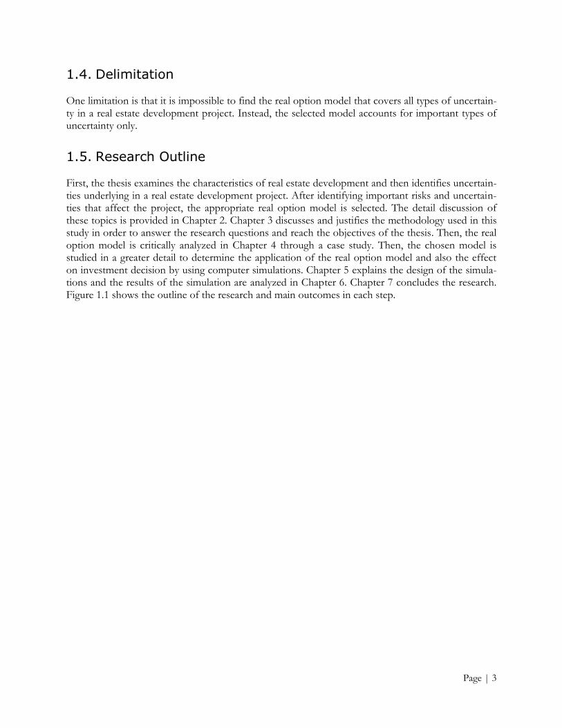
First, the thesis examines the characteristics of real estate development and then identifies uncertain-ties underlying in a real estate development project. After identifying important risks and uncertain-ties that affect the project, the appropriate real option model is selected. The detail discussion of these topics is provided in Chapter 2. Chapter 3 discusses and justifies the methodology used in this study in order to answer the research questions and reach the objectives of the thesis. Then, the real option model is critically analyzed in Chapter 4 through a case study. Then, the chosen model is studied in a greater detail to determine the application of the real option model and also the effect on investment decision by using computer simulations. Chapter 5 explains the design of the simula-tions and the results of the simulation are analyzed in Chapter 6. Chapter 7 concludes the research. Figure 1.1 shows the outline of the research and main outcomes in each step.

Page | 4

Figure 1.1 Research Outline

Analyze the Real Option Model in Detail through a Case Study

Study the Applications and Ef-fect of the Real Option Model

in Investment Decision

Examine Characteristic of Real Estate Development

Identify Uncertainties in Real Estate Development

Select a Real Option Model that Captures Identified Uncertain-

ties

Analyze and Summarize the Result

Real Option Model

Answering the first research question: “What are the main concerns needed to be considered when using real options to evaluate real estate develop-

ment projects under uncertainties?”

Answering the second research question: “How do real options affect investment decision in real

estate development projects under uncertainties?”

Outcomes Research Outline

Page | 5

2. Theory and Literature Review

This chapter reviews the existing body of knowledge related to the thesis in order to provide the background knowledge for the readers. In addition, the thesis uses the theories presented in this chapter as ground knowledge to conduct the study that answers the research questions.

2.1. Real Estate Development Investment

This section provides the knowledge of real estate development. First, it examines the macro picture of real estate system in order to understand how the system works and how each element in the sys-tem connects to the real estate development. Then, the section focuses on the real estate develop-ment process in order to identify the criteria used to decide whether to invest in a project or not. The last part discusses risks and uncertainties that affect the decision making criteria and identifies the important uncertainties needed to be considered when evaluating a real estate development pro-ject.

2.1.1. Real Estate Development as Part of Real Estate System

In real estate system, there are three major elements that interact together. These elements are space market, asset market and real estate development industry.

To begin with the markets in real estate system, a market is a mechanism which goods and services are exchanged among different owners (Geltner et al., 2006, p. 3). In real estate context, a real estate property is a product that can be traded or provide a service in the market as well. Here are the characteristics of space market and asset market in the real estate system.

Space Market

The space market is the market for the usage or right to use the space of real property, land and built space (Geltner et al., 2006, p. 3). The demand side of this market is individuals, families, or organiza-tions that want to use the space of the real property for living or production purposes. On the other side, the suppliers of the space market are the property owners who rent their property to tenants. These consumers are required to pay the rent for using the space every certain period of time such as monthly or yearly. The rent is normally quoted in price per m2.

In general, the rental price of a property is a good indicator in the level of balance in demand and supply of space market and more importantly, the value of the property that is being rented. The rental price depends on various parameters. The research of Marco (2008) on determining the fac-tors that affect the residential rental price in New York City reveals that there are many factors af-fecting the rental price. These are environmental regulatory and economic factors namely, location of the property, crime rates in the area, rent-regulated or rent-subsidized housing, and household incomes. Another research by Donovan and Butry (2011) focused on the relationship between ur-ban trees and rental price of single-family homes in Portland, Oregon, US. They found a positive correlation between these two parameters which is additional trees in house’s lot and public right of way increased the monthly rental price by $5.62 and $21.00 respectively. When considering commer-

Page | 6

cial real estate rental pricing, Wiley, Benefield and Johnson (2010) presented that the energy-efficient design of the commercial office space earns superior rents and sustains higher occupancy.

The amount of rental payment is very important in real estate system context since it is the main cash flow that involves in this market and has the direct effect on another market in real estate sys-tem which is the asset market.

Asset Market

The real estate asset market is the market for the ownership of real estate assets (Geltner et al., 2006, p. 11). The real estate assets include land parcels and property (buildings) that are built on the lands. The supply side of real estate assets is the property owners who want to sell their assets. On the de-mand side, it is the investors who want to buy in order to increase the holding on their real estate assets. Owning real estate assets means having the claim of future cash flows that the assets can gen-erate. These future cash flows normally come in two forms which are the rental payments of the space market that was mention earlier and the sales of the property (Miles et al., 2007). With this characteristic, real estate assets can be viewed as another type of capital assets, such as stocks or bonds, in a larger capital market. As same as all types of investments, when investors want to invest in any particular capital assets, they need to price those assets first before deciding to invest. There are several ways that real estate assets can be priced.

There are many factors that affect the value of real estate assets. Geltner et al. (2006, p. 14-15) identi-fied that opportunity cost of capital, growth expectations on rental prices, and investor risk percep-tion influence the capitalization rate using for evaluating real estate asset values. Moreover, Hott (2011) explained that mortgage lending behavior of banks affects the real estate prices. This is be-cause real estate prices depend on the level of demand of the property which links together with the level of supply of mortgages for the investors. The research from Wang, Yang and Liu (2011) exam-ined the linkage between urban economic openness, the ratio of trade volume as a percentage of GDP, and urban real estate prices. They empirically found that for every 1% increase in urban eco-nomic openness, urban real estate prices will increase significantly by 0.282% and urban economic openness alone accounted for about 15.90% appreciations of Chinese real estate prices. This can be summarized that economic factor affects the real estate asset prices.

To sum up, the main focus on the asset market that investors need to consider is the value of real estate assets. The asset values are also influenced by the space market through the rental price and other factors. The property values play an essential role in the real estate development industry in the next part.

Real Estate Development Industry

Real estate development industry is both supplier and the first owner of real estate assets that can be sold or provide the service in both space market and asset market. The main role of the real estate developers is to convert financial capital into physical capital (Geltner et al., 2006, p. 21) in order to supply the demand from both markets. For this, the key question that real estate developers have to consider is that “is a development worth undertake and profitable or not?” The next section dis-cusses in a greater detail of real estate development in order to determine the key step that answers this question and elements that influence the decision to invest in a project.

Page | 7

Real Estate System

Putting all elements together, the real estate system can be displayed by Figure 2.1. It also shows the connection and logical flow between each component as described earlier in the previous parts. This gives the broad perspective on how real estate development (which is the focus of this research) is affected by different factors in the system.

Figure 2.1 Real Estate System (Geltner et al., 2006, p. 23)

2.1.2. Real Estate Development Process

Miles et al. (2007, p. 5) define the definition of real estate development as the following.

“A real estate development starts as an idea that comes to fruition when consumers - tenants or owner-occupants - occupy the bricks and mortar (space) put in place by the development team.

Page | 8

Land, labor, capital, management, entrepreneurship, and broadly defined partnerships are needed to transform an idea into reality. Value is created by providing usable space over time with associated services. It is these three things - space, time, and services - in association that are needed so con-sumers can enjoy the intended benefits of the built space.”

Real estate developers follow a sequence of steps starting from recognizing the need in the market to completing the construction and managing it. All of the important steps are captured in the eight-stage model of real estate development (Miles et al., 2007, p. 7) in Figure 2.2.

Figure 2.2 The Eight-Stage Model of Real Estate Development (Miles et al., 2007, p. 7)

Page | 9

From the model in Figure 2.2, it is obvious that the third stage which is the feasibility analysis is the core step used to answer the question “is a development worth to undertake and profitable or not?” which is the key question for the developers. When considering more carefully, the feasibility analy-sis is also a very important stage of the whole process since it is the key decision making point that has the effect in the long term. One reason is because of the characteristic of this type of investment that is characterized by large capital funding, long construction period, slow payback and enduring many uncertainties(Rocha et al., 2007; Mao and Wu, 2011; Bulan, Mayer and Somerville 2006). Fur-thermore, after the evaluating stage of the project, the capital investment and operational costs in the following steps increase significantly compared with the previous steps (for example, these costs are legal and administrative cost, construction cost, and marketing cost). These steps also involve many external parties such as legal, local government, and construction companies. These create much higher complexity in managing and execution.

Graaskamp (1972) defines that a real estate development project is feasible when there is a reasona-ble likelihood of satisfying explicit objectives form the selected plan within the constrains and lim-ited resources. With this definition, it shows that there are several topics that are needed to be cov-ered in a feasibility analysis. Miles et al. (2007) provide a layout that covers essential elements in fea-sibility analysis as follows.

Executive summary

Maps

Photographs of the site

Renderings

Market study

Electronic valuation model derived from market study

Documented cost projections

Development schedule

Background on key players, including project consultants

Although there are many aspects needed to be covered in feasibility analysis, the bottom line decid-ing whether the project is feasible or not is still financial aspect of the analysis as Miles et al. (2007, p. 413) mentioned “a project is feasible when the value exceeds all the projected costs of develop-ment.”

Regarding the costs of the project, each project has different cost structure which depends on the characteristic of the project such as size, or real estate type. In general, Miles et al. (2007, p. 406) pro-vides the list of costs in a real estate development project as follow.

Land cost

Site and infrastructure development costs

Design fees

Architecture

Engineering

Hard costs

By category

Page | 10

Labor and materials

Permitting costs

Financial costs

Permanent loan commitment fees

Construction interest

Construction loan fees

Marketing costs

Promotion

Advertising

Leasing commissions

Brokers’ fees

Preopening operating costs

Legal fees

Accounting costs

Field supervision (inspection) costs

Overhead

Contingencies

Development fees

Regarding the value of the project, it can be determined through the market study. The market study is the most crucial item in feasibility analysis and considers as a backbone of the real estate develop-ment process (Miles et al. 2007, p. 415). The market study analyses all long term economic trends from global to local perspective and also the demand and supply of real estates in space market. The end result of the market study is the forecast of expected income from rents (price per m2). This is used to derive the cash flows that the project can generate and ultimately, the value of the project (Miles et al. 2007, p. 395-396, 415-417).

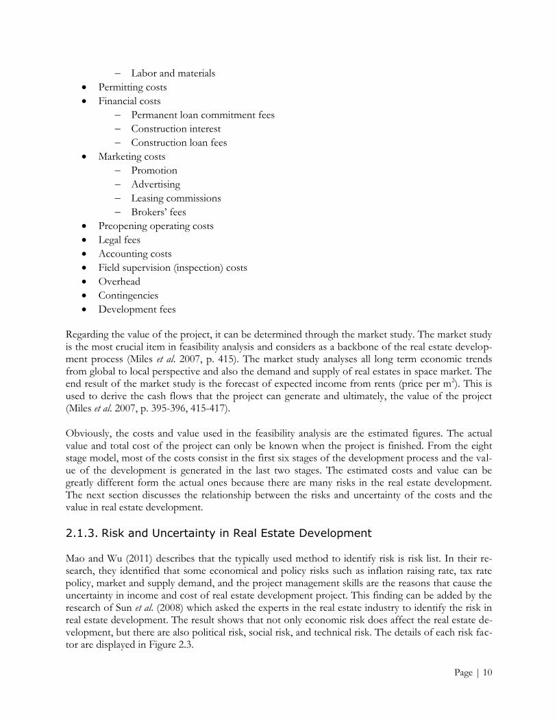
Obviously, the costs and value used in the feasibility analysis are the estimated figures. The actual value and total cost of the project can only be known when the project is finished. From the eight stage model, most of the costs consist in the first six stages of the development process and the val-ue of the development is generated in the last two stages. The estimated costs and value can be greatly different form the actual ones because there are many risks in the real estate development. The next section discusses the relationship between the risks and uncertainty of the costs and the value in real estate development.

2.1.3. Risk and Uncertainty in Real Estate Development

Mao and Wu (2011) describes that the typically used method to identify risk is risk list. In their re-search, they identified that some economical and policy risks such as inflation raising rate, tax rate policy, market and supply demand, and the project management skills are the reasons that cause the uncertainty in income and cost of real estate development project. This finding can be added by the research of Sun et al. (2008) which asked the experts in the real estate industry to identify the risk in real estate development. The result shows that not only economic risk does affect the real estate de-velopment, but there are also political risk, social risk, and technical risk. The details of each risk fac-tor are displayed in Figure 2.3.

Page | 11

Figure 2.3 Risk Factors in Real Estate Development (Sun et al., 2008)

When considering the level of impact of each risk on real estate development, the result can be found in Linjie (2010) study. He asked industry experts, professors and practitioners, to evaluate the impact of different types of risk on real estate development by categorizing into seven levels as [VL] (very low), [L] (low), [RL] (rather low), [M] (neither high nor low), [RH] (rather high), [H] (high), and [VH] (very high). Table 2.1 shows the results of the study.

Table 2.1 Impact of Risks on Real Estate Development (Linjie, 2010)

Now, it can be clearly seen that there are many types of risk that have different levels of impact on real estate development projects. These risks consist in all of the stages of the development process and also are the main cause, directly and indirectly, of the uncertainty in both cost and value of the

Page | 12

project. Putting all of these together, Figure 2.4 can be drawn to show the linkage between the eight stage model of real estate development, risks, and uncertainty in the cost and value.

Figure 2.4 Relationships between Real Estate Development, Risk, and Uncertainties

The uncertainty in the cost and the value of real estate development affect considerably in the feasi-bility analysis because it can turn a feasible project into a non-profitable project at the end. On ac-count of this, the evaluation method used in the feasibility analysis needs to take these types of un-certainty into the consideration. This leads to the next section of the thesis that focuses on finding the real option models that capture these two types of uncertainty, cost uncertainty and value uncertainty, for the evaluation of real estate development.

Cost Uncertainties

Contract Negotiation

Inception of Idea

Refinement of the Idea

Feasibility (Key Decision Point)

Formal Commitment

Construction

Completion and Formal Opening

Property, Asset, and Portfolio Management

Value Uncertainties

Real

Est

ate

Deve

lop

men

t P

rocess

Risk Factors

Economical Risk

Political Risk

Technical Risk

Social Risk

Project Risk

Other Risks

Affect

Page | 13

2.2. Determining Cost and Value of Project

As mentioned in the section 2.1.2, it discussed roughly on how to determine the costs and the value of real estate investment project. In this part, it examines in greater detail on how real estate devel-opers can calculate the costs and the value of the project more precisely.

Williams (1991) discusses that investors can choose to develop a property with a certain density ( ) which is subject by the zoning regulations. The density means the available space that the building will have after finishing the construction. From the basis of this concept, Williams (1991), Quigg (1993), and Sing (2001) said that the cost and the value of the real estate development project can be determine in relationship with the density function.

2.2.1. Determining Cost

According to the list of the costs in section 2.1.2, these costs can be separated into fixed costs and variable costs. The fixed costs are the costs that do not change according to the size or the height of the construction. Here is the example of the fixed costs.

Land cost

Design fees

Architecture

Engineering

Permitting costs

Financial costs

Permanent loan commitment fees

Construction interest

Construction loan fees

Marketing costs

Promotion

Advertising

Leasing commissions

Brokers’ fees

Preopening operating costs

Legal fees

Accounting costs

Field supervision (inspection) costs

Overhead

Contingencies

Sing (2001) mentioned that the largest fixed cost in real estate development is the land cost. For the variable costs, this type of costs changes in the relationship with the density of the building. Below is the example of the variable costs in a real estate development project.

Site and infrastructure development costs

Page | 14

Hard costs

By category

Labor and materials

Overhead

Development fees

Additionally, Sing (2001) also mentioned that when building reaches a certain size or gets taller, the variable costs, especially the construction cost, increase considerably with every additional unit in-creased in building height. With all of these, Williams (1991), Quigg (1993), and Sing (2001) deter-mined the total cost in a real estate development project as the following function.

(1)

Where is the cost of the development project

is the density of the building (m2)

is the cost elasticity of scale

is the unit variable cost per unit of density, and

is the total fixed cost

The variable which is the cost elasticity of scale represents what Sing (2001) mentioned and > 1 when the development is at high density (Williams, 1991).

2.2.2. Determining Value

Regarding the value of the project, as mentioned in previous section, the value of the project de-pends on the expected income in term of rental which is quoted in price per m2. With this, the value of the development project can be determined as a function of the density and rental price as follow (Williams, 1991).

(2)

From the above equation, Sing (2001) added the price elasticity of scale into the function. So, the final form of the equation is displayed below.

(3)

Where is the income of the development project at year

is the density of the building (m2)

is the price elasticity of scale, and

is the rental price per m2

The rental price, , changes according to the demand and supply in the space market and also eco-nomic situation in certain period of time. This value can be determined through the market study or examining the current market price of the area that the investor wants to develop the real estate.

Since is quoted as a rental price per year, in order to find the total present value that the project

Page | 15

can generate, this stream of cash flows has to be discounted back to the present value. A real estate can be considered as perpetuity project because once finish constructing, the building has an infinite life time that can generate cash flow to the owner. On account of this, the present value can be cal-culated with this formula.

∑

(4)

This formula can be reduced into the short form as shown in the equation (5) (Brealey, Meyers and Allen, 2006, p. 37).

(5)

Where is the expected rate of return on rent (%)

2.3. Real Options in Real Estate Development

This section describes real estate development investment evaluation. At the beginning of the sec-tion, general concepts of real options are introduced. After providing the basic concepts of real op-tions, the section focuses on identifying types of real option that consist in real estate development. Then, the existing real option model that captures the important uncertainties in the real estate de-velopment project is selected.

2.3.1. Real Options

Financially, options are financial instruments mostly used in stock trading. Options are the “right” but not “obligation” to buy or sell the share at a specific price (exercise or strike price) on or before a specific date. The options that allow investors to buy a share at a specific price in the future are called call options (in short for calls). On the contrary, the options that allow investors to sell a share at a specific price in the future are called put options (in short for puts). Furthermore, if call or put options can be exercised on a particular date only, they are known as European options. If the op-tions can be exercised on or any dates before a particular date, these options are American options. Both calls and puts have a great value for the stock traders since they have the application to hedge the risk and protect the possible losses due to uncertainties in the future of shares.

Myers (1977) is the first one who identified the same application of financial options in capital in-vestment projects. The term for this type of options is real options. He stated that an investment opportunity in the future can be viewed as an American call option. This reflects the management flexibility to modify the projects before and after investing in the project. Managers have the right but not the obligation to whether defer, expand, or abandon a project which depends on the situa-tion in the future. Together with the concept of financial options and real options, the analogies be-tween the elements in these two types of options can be drawn as presented in Table 2.2 (Brach, 2003, p. 43).

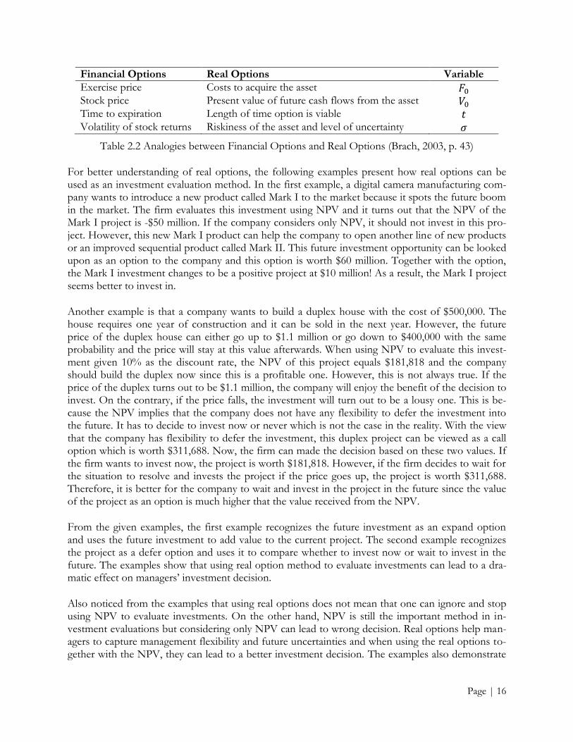
Page | 16

Financial Options Real Options Variable

Exercise price Costs to acquire the asset Stock price Present value of future cash flows from the asset Time to expiration Length of time option is viable Volatility of stock returns Riskiness of the asset and level of uncertainty

Table 2.2 Analogies between Financial Options and Real Options (Brach, 2003, p. 43)

For better understanding of real options, the following examples present how real options can be used as an investment evaluation method. In the first example, a digital camera manufacturing com-pany wants to introduce a new product called Mark I to the market because it spots the future boom in the market. The firm evaluates this investment using NPV and it turns out that the NPV of the Mark I project is -$50 million. If the company considers only NPV, it should not invest in this pro-ject. However, this new Mark I product can help the company to open another line of new products or an improved sequential product called Mark II. This future investment opportunity can be looked upon as an option to the company and this option is worth $60 million. Together with the option, the Mark I investment changes to be a positive project at $10 million! As a result, the Mark I project seems better to invest in.

Another example is that a company wants to build a duplex house with the cost of $500,000. The house requires one year of construction and it can be sold in the next year. However, the future price of the duplex house can either go up to $1.1 million or go down to $400,000 with the same probability and the price will stay at this value afterwards. When using NPV to evaluate this invest-ment given 10% as the discount rate, the NPV of this project equals $181,818 and the company should build the duplex now since this is a profitable one. However, this is not always true. If the price of the duplex turns out to be $1.1 million, the company will enjoy the benefit of the decision to invest. On the contrary, if the price falls, the investment will turn out to be a lousy one. This is be-cause the NPV implies that the company does not have any flexibility to defer the investment into the future. It has to decide to invest now or never which is not the case in the reality. With the view that the company has flexibility to defer the investment, this duplex project can be viewed as a call option which is worth $311,688. Now, the firm can made the decision based on these two values. If the firm wants to invest now, the project is worth $181,818. However, if the firm decides to wait for the situation to resolve and invests the project if the price goes up, the project is worth $311,688. Therefore, it is better for the company to wait and invest in the project in the future since the value of the project as an option is much higher that the value received from the NPV.

From the given examples, the first example recognizes the future investment as an expand option and uses the future investment to add value to the current project. The second example recognizes the project as a defer option and uses it to compare whether to invest now or wait to invest in the future. The examples show that using real option method to evaluate investments can lead to a dra-matic effect on managers’ investment decision.

Also noticed from the examples that using real options does not mean that one can ignore and stop using NPV to evaluate investments. On the other hand, NPV is still the important method in in-vestment evaluations but considering only NPV can lead to wrong decision. Real options help man-agers to capture management flexibility and future uncertainties and when using the real options to-gether with the NPV, they can lead to a better investment decision. The examples also demonstrate

Page | 17

that different types of real option have different usage in investment evaluation. On account of this, it is essential to determine which types of real option needed to be considered in an investment.

With the benefits of the real option that captures managerial flexibility, it has been found that real options have been used in many different industries. For the oil industries, real options can also be used since the oil production and exploration projects require large capital investment with high fluctuation in the oil price and endure many uncertainties (Cortazar and Schwartz, 1997; Armstrong et al., 2004; Dias, 2004; Fan and Zhu, 2010). Duku-Kaakyire and Nanang (2004) and also Kallio, Kuula and Oinonen (2012) used real options for forestry investment analysis. In Duku-Kaakyire’s and Nanang’s (2004) paper, they discussed that there are four types of real option which are the op-tion to delay, expand, abandon, and multiple options. They concluded that real option method give a better decision since the method values management flexibility, risks, and uncertainties in the pro-ject. Furthermore, Cassimon et al. (2011) presented models used for pharmaceutical R&D licensing opportunities. Their study introduced real option model capturing technical risk of new drug devel-opment. Then, the study concluded that the NPV can underestimate the value of the project, while the real option evaluation reflects the nature of R&D investment in a better way. So, the real option approach is more reliable than the NPV. Not only can the real option be used solely as investment evaluation tools, it can also be used together with other frameworks such as Mean-Variance (MV), portfolio management analysis, and risk-return tradeoff as presented in the studies of Wu and Ong (2008) and Choungsirakulwit and Sutivong (2007).

After understanding the general concepts of real options, the effect of the real options in investment evaluation, and the applications of real options in different industries, the next part discusses the types of real option that can be found in real estate development which is the focus of the thesis.

2.3.2. Real Options in Real Estate Development

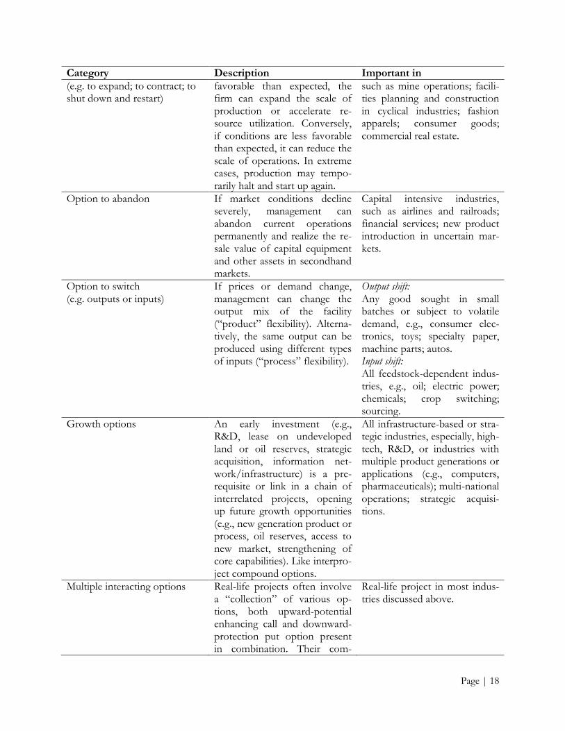
Trigeorgis (2001, p. 104-105) described that there are seven most common types of real options that can be found in any investments. Also, he specified the types of industries that these options are im-portant in as presented in Table 2.3.

Category Description Important in

Option to defer Management hold a lease on (or an option to buy) valuable land or resources. It can wait (x years) to see output price justify constructing a building or plant, or developing a field.

All natural resource extracting industries; real estate develop-ment; farming; paper products.

Time to build option (staged investment)

Staging investment as a series of outlays creates an option to abandon an enterprise in mid-stream if new information is unfavorable. Each stage can be viewed as an option on the val-ue of subsequence stages, and valued as a compound option.

All R&D intensive industries, especially pharmaceutical; long-development capital intensive projects, e.g. large-scale con-struction or energy generating plants; start-up ventures.

Option to alter operating scale If market conditions are more Natural resource industries

Page | 18


(e.g. to expand; to contract; to shut down and restart)

favorable than expected, the firm can expand the scale of production or accelerate re-source utilization. Conversely, if conditions are less favorable than expected, it can reduce the scale of operations. In extreme cases, production may tempo-rarily halt and start up again.

such as mine operations; facili-ties planning and construction in cyclical industries; fashion apparels; consumer goods; commercial real estate.

Option to abandon If market conditions decline severely, management can abandon current operations permanently and realize the re-sale value of capital equipment and other assets in secondhand markets.

Capital intensive industries, such as airlines and railroads; financial services; new product introduction in uncertain mar-kets.

Option to switch (e.g. outputs or inputs)

If prices or demand change, management can change the output mix of the facility (“product” flexibility). Alterna-tively, the same output can be produced using different types of inputs (“process” flexibility).

Output shift: Any good sought in small batches or subject to volatile demand, e.g., consumer elec-tronics, toys; specialty paper, machine parts; autos. Input shift: All feedstock-dependent indus-tries, e.g., oil; electric power; chemicals; crop switching; sourcing.

Growth options An early investment (e.g., R&D, lease on undeveloped land or oil reserves, strategic acquisition, information net-work/infrastructure) is a pre-requisite or link in a chain of interrelated projects, opening up future growth opportunities (e.g., new generation product or process, oil reserves, access to new market, strengthening of core capabilities). Like interpro-ject compound options.

All infrastructure-based or stra-tegic industries, especially, high-tech, R&D, or industries with multiple product generations or applications (e.g., computers, pharmaceuticals); multi-national operations; strategic acquisi-tions.

Multiple interacting options Real-life projects often involve a “collection” of various op-tions, both upward-potential enhancing call and downward-protection put option present in combination. Their com-

Real-life project in most indus-tries discussed above.

Page | 19


bined option value may differ from the sum of separate op-tion values, i.e. they interact. They may also interact with fi-nancial flexibility options.

Table 2.3 Common Types of Real Options and Industries Consisting These Options (Trigeorgis, 2003, p. 104-105)

From the definition of each type of option given by Trigeorgis (2003, p. 104-105) in Table 2.3, there are two types of options that are mentioned to be important in real estate development, option to defer and option to alter operating scale. But, the thesis focuses only on option to defer with the fol-lowing reasons.

Option to defer - This type of option is common in real estate development since a compa-ny can purchase a land space and wait to build any real estate on that land at any time it wants according to the market situation. The company does not have to build a real estate asset immediately because it does not cost more or the land will not deteriorate through time. The defer option of real estate development is recognized in some research articles as well. Sing (2001) identified that a land parcel entails not only the net value of real estate asset that can be built on the land, but it also includes the premium for the option to wait to de-velop the land (to defer the investment). This is supported by Cappoza and Sick (1992) and Quigg (1993) that say the current time does not always to be an optimal time to invest in a real estate project. So, the project should be deferred to the future.

Option to alter operating scale - Although the option to alter operating scale is mentioned to be important in commercial real estate according to Table 2.3, there are no research articles that support this type of option properly. Furthermore, a real estate project cannot be altered in term of scale easily (increase or decrease the available space). This is because any construc-tion developments have to follow the construction drawing and the contract that was agreed before. Moreover, there are zoning regulations that developers have to follow. Once the company starts to develop a real estate project in a particular area, the building cannot be easily changed because of the regulations (Williams, 1991). On account of this, the option to alter operating scale is not considered in this thesis.

In the next section, the thesis identifies the mathematical model that is used to find the value of the option to defer. The identified model has to take two types of uncertainty which are value uncertain-ty and cost uncertainty into the account since these uncertainties are important in real estate devel-opment (as mentioned in the section 2.1.3).

2.3.3. Option to defer

Option to defer has been examined in several articles. Titman (1985) presented a simple model to evaluate a real estate investment on vacant land when the value of the building and the size are un-certain. Also, Paddock, Siegel, and Smith (1988) developed a model to value a claim on a real asset by focusing on the case of offshore petroleum lease. However, the model proposed by Titman (1985) is quite simple since is not a continuous time model. The model consists only two dates (pre-

Page | 20

sent date and a future date), so the land developer has only two decision points. This is not a realistic assumption. Another model that Paddock, Siegel, and Smith (1988) presented is too industry specif-ic. For this, it is difficult to adapt the model in the real estate development context.

Due to these reasons, the thesis chooses the model from McDonald and Siegel (1986). This model evaluates the value of waiting to invest and it is suitable in this study because the model captures both value and cost uncertainties. Furthermore, the model has a general purpose that can be imple-mented in real estate development. The following is the description of the model.

At the beginning, the model assumes that at any time , the firm can invest in a project that costs

and the project has the present value at . Both and follow geometric Brownian motion with drift below.

(6a)

(6b)

Where and are the change in the project value and cost

and are the drift in the project value and cost (%)

and are the degree of uncertainty (volatility) of the project value and cost (%)

is the time interval during the observed period, and

and are standard Wiener process (Brownian motion).

The assumption that the value and the cost of the project move stochastically as geometric Browni-an motion is acceptable. The main driver of the project value is price per m2 while there is no single parameter that represents the cost but most of the costs in real estate development are land price and construction material such as iron and concrete which are similar to commodities. Table 2.4 compares the definition of geometric Brownian motion with drift (Dixit and Pindyck, 1994, p. 63, 71) with the value (price per m2) and the cost (construction materials) of the project.

Geometric Brownian Motion with Drift Characteristic (Dixit and Pindyck, 1994, p. 63, 71)

Price per m2 behavior in a real estate development pro-ject

Construction material behav-ior in a real estate develop-ment project

The Brownian motion is a con-tinuous-time stochastic process. The stochastic process is a vari-able that changes over time in a random way.

Price per m2 in the market changes along the time in a random way with a certain di-rection (the drift). For example, the price of the area has the overall trend to increase during a period of time (a positive drift) but during this period, it fluctuates in a random way.

Price of construction materials change along the time in a ran-dom way with a certain direc-tion (the drift). For example, the price of construction mate-rial can have the overall trend to increase (a positive drift) but the price is still fluctuated in random way.

The probability of distribution of all future values of the pro-

The area price of the property tomorrow depends on today’s

The price of construction mate-rials in tomorrow depends on

Page | 21

Geometric Brownian Motion with Drift Characteristic (Dixit and Pindyck, 1994, p. 63, 71)

Price per m2 behavior in a real estate development pro-ject

Construction material behav-ior in a real estate develop-ment project

cess depends only on its current value, and it is unaffected by any past values of the process or by any other of the current information. For this, in order to forecast the future value of a variable, it requires only one current value of the variable.

price only. today’s price only.

The Brownian motion has in-dependent increments. This means that the probability dis-tribution for the change in the process over any time interval is independent of any other (overlapping) time interval.

The chance that the price per m2 will go up or down has the same probability and the degree of change is normally distribut-ed. This means that there is a higher probability that the price will go up or down with in one standard deviation and a lower probability that the price will change within three standard deviations (but it is possible to happen).

The chance that the construc-tion material price will go up or down has the same probability and the degree of change is normally distributed. This means that there is a higher probability that the price will go up or down with in one stand-ard deviation and a lower prob-ability that the price will change within three standard deviations (but it is possible to happen).

Changes in the process along the time are lognormally dis-tributed.

The changes of price per m2 are lognormally distributed, which means that, in the worst case, the price never decreases more than 100 percent (the price equals to zero), but it can in-crease more than 100 percent.

The price of the construction materials are lognormally dis-tributed, which means, the cost never decreases more than 100 percent and becomes negative value, while there is no limit of the increase in the value.

Table 2.4 Relationship between geometric Brownian motion with drift, price per m2, and construc-tion materials

Figure 2.5 shows the sample part of geometric Brownian motion with drift for the better under-standing in the movement of these two factors.

Page | 22

Figure 2.5 Sample path of geometric Brownian motion with drift (Dixit and Pindyck, 1994, p. 73).

In addition, the model assumes that the investment opportunities are infinitely lived. This assump-tion also matches the real estate development characteristic because in order to build a property on the land, the developer has to acquire the land. After acquiring, the land does not have expiration date in the future, so the investment opportunity to develop a real estate is infinitely lived.

After taking these assumptions in mind, McDonald and Siegel (1986) derived the model that values the opportunity to invest in the future as following.

(

)

(7)

Where

(8)

√(

)

(

) (9)

(10)

Given is the option value

is the expected rate of return on asset (%)

is the expected rate of return on asset (%), and

is the instantaneous correlation between the drift rate of and

Page | 23

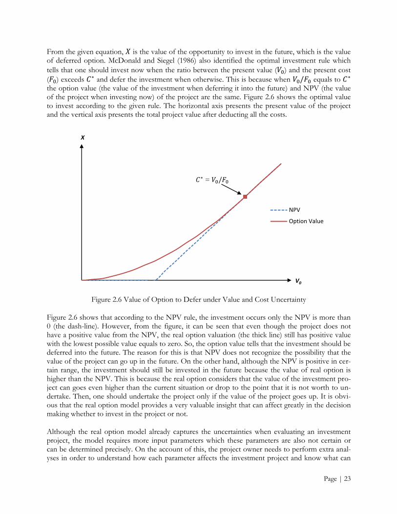
From the given equation, is the value of the opportunity to invest in the future, which is the value of deferred option. McDonald and Siegel (1986) also identified the optimal investment rule which

tells that one should invest now when the ratio between the present value ( ) and the present cost

( ) exceeds and defer the investment when otherwise. This is because when equals to the option value (the value of the investment when deferring it into the future) and NPV (the value of the project when investing now) of the project are the same. Figure 2.6 shows the optimal value to invest according to the given rule. The horizontal axis presents the present value of the project and the vertical axis presents the total project value after deducting all the costs.

Figure 2.6 Value of Option to Defer under Value and Cost Uncertainty

Figure 2.6 shows that according to the NPV rule, the investment occurs only the NPV is more than 0 (the dash-line). However, from the figure, it can be seen that even though the project does not have a positive value from the NPV, the real option valuation (the thick line) still has positive value with the lowest possible value equals to zero. So, the option value tells that the investment should be deferred into the future. The reason for this is that NPV does not recognize the possibility that the value of the project can go up in the future. On the other hand, although the NPV is positive in cer-tain range, the investment should still be invested in the future because the value of real option is higher than the NPV. This is because the real option considers that the value of the investment pro-ject can goes even higher than the current situation or drop to the point that it is not worth to un-dertake. Then, one should undertake the project only if the value of the project goes up. It is obvi-ous that the real option model provides a very valuable insight that can affect greatly in the decision making whether to invest in the project or not.

Although the real option model already captures the uncertainties when evaluating an investment project, the model requires more input parameters which these parameters are also not certain or can be determined precisely. On the account of this, the project owner needs to perform extra anal-yses in order to understand how each parameter affects the investment project and know what can

0

20

40

60

80

100

120

140

0 20 40 60 80 100 120 140 160 180 200

X

V0

NPV

Option Value

𝐶 = 𝑉 𝐹

Page | 24

happen in the future. The next section discusses the key methods that are used to perform this kind of the analysis.

2.4. Financial Analysis with Uncertain Variables

In this section, it discusses the methods that are used to analyze investment projects when there is uncertainty in input parameters. The section focuses on the two most recognized approaches in cor-porate finance namely, sensitivity analysis and Monte Carlo simulation.

2.4.1. Sensitivity Analysis

“Uncertainty means that more things can happen than will happen.” (Brealey, Meyers, and Allen, 2006, p. 255). This definition is what sensitivity analysis tries to answer. The sensitivity analysis does not focus on answering what will happen to an investment project, but it rather examines what can actually happen to the project in different situations. The sensitivity analysis can be performed by changing some input parameters or one parameter at a time in a certain range while keeping other parameters unchanged. Then, it calculates all of the possible project values according to the changed parameter(s). The process in performing sensitivity analysis forces the project owner to identify all key variables used in the calculation and to determine which input parameters are most likely to de-viate from the estimated values.

Sensitivity analysis has many benefits and applications. One application of the sensitivity analysis is to find the pessimistic and optimistic scenario of a project. This can be done by asking relevant de-partments involving in the project to provide not only the estimated figures, but also to submit the pessimistic and optimistic number for the underlying variables. This helps the analyst to know the possible spread of the project value so that he/she realizes the risk level of the project from mises-timating the variables. Moreover, this application of sensitivity analysis reveals the main source of uncertainty causing the pessimistic scenario. Hence, the company can take a corrective action to re-solve the uncertain situation before actually invest in the project (Brealey, Meyers, and Allen, 2006, p. 255-257).

For example, a car manufacturing company wants to introduce new electric scooter to the market. The company calculates the NPV of the project and the result is $15 million. The company per-forms the sensitivity analysis and found out that the main drivers used in the calculation are new product’s share of the market and the unit production cost of the scooter. So, the finance depart-ment asked the marketing and manufacturing department to estimate the pessimistic and optimistic figures of the market share and unit production cost to the department. With these figures, the NPV of the project turns out to be -5$ million and $30 million in pessimistic and optimistic scenario re-spectively. In addition, the company also found out that the pessimistic scenario in unit production cost is caused by the concern from manufacturing department that the new machine used in the production will not work properly as designed. This leads to an increase in unit production cost of the scooter. To resolve the issue, the company decides to run a pretest on the machine with some cost which reduces the uncertainty in this variable. As a result, the pessimistic scenario turns out to be 1$ million and this tells that the company is unlikely to be in a trouble in the project nevertheless there are some uncertainties remaining.

Page | 25

However, the mentioned application of the sensitivity analysis has some limitations. First, the results from the analysis are somewhat ambiguous because pessimistic and optimistic are subjective which leaves the room for different interpretation. One person pessimistic scenario can still be considered as a normal situation or even optimistic to another one. Another drawback of the sensitivity analysis is that the underlying variables are likely to be interrelated such as an increase in market share can lead to an increase in unit sale price. Changing the variables separately causes unreliable results in the sensitivity analysis as well (Brealey, Meyers, and Allen, 2006, p. 257-258).

Break-even analysis is another application of sensitivity analysis. In this case, the objective of the analysis is to find the value of a particular input parameter that makes the project to become feasible, or NPV equals to zero. From the previous example, the company can use break-even analysis to find how many scooters needed to be sold per year so that the project becomes profitable. Also, the company can run the analysis to identify the minimum price per unit of scooter should be sold to the market in order to yield a positive NPV. This type of sensitivity analysis gives different perspec-tive to the project owner on how the company can earn a profit from the investment (Brealey, Mey-ers, and Allen, 2006, p. 259-261).

Last but not least, sensitivity analysis helps the analyst to understand how each variable affects the project and in what degree. Results from the analysis provide an in-depth understanding of the valu-ation model that is used to calculate the project value. The degree of the effect on the project value can be considered as a signal that gives a caution to the project analyst on which variable should be carefully estimated and monitored.

2.4.2. Monte Carlo Simulation

Sensitivity analysis is a very useful tool used in financial analysis when input variables are uncertain. However, sensitivity analysis only allows the effects of changing one variable at a time to be consid-ered and also the limited number of scenarios can be generated through this method (Brealey, Mey-ers, and Allen, 2006, p. 263). This is because changing many variables or creating a great number of scenarios brings complexity to the analysis which leads to unreliable result. Furthermore, as men-tioned earlier, sensitivity analysis ignores that the variables are likely to be interrelated and interde-pendent between different periods of time. This is quite a strong assumption that does not reflect the reality.

With these pitfalls, an alternative is to use computer simulation in the financial analysis when there are uncertainties in input variables. Monte Carlo Simulation is a widely recognized tool that was in-troduced in capital budgeting problems by Hertz (1968). The Monte Carlo simulation can generate all possible combinations of inputs and therefore, it can generate the entire distribution of the possi-ble outcomes (Brealey, Meyers, and Allen, 2006, p. 263). Moreover, the Monte Carlo simulation as-sists the decision makers to be more rational and consistent in their decisions and the analysts to gain a greater comprehensiveness and understanding in all of the risk factors in the development project (Loizou and French, 2012).

Loizou and French (2012) and Brealey, Meyers, and Allen (2006, p. 263-268) described how to con-struct a Monte Carlo simulation which has three main steps as the following framework.

Page | 26

Step 1: Modeling the investment project

The first step of the simulation is to give a precise model of the project to a computer. The model in this case is normally a mathematical formula. For example, a company wants to run a Monte Carlo simulation on the electric scooter project to see all of the possible cash flow. The company specifies the model of cash flow as follow.

Cash flow = (revenue - costs - depreciation) (1 - tax rate) + depreciation

Revenues = market size market share unit price

Costs = (market size market share unit price) + fixed cost

In this step, not only does the company specify the model of the cash flow, but it also has to identify the interrelation between the variables in the model. Using the same example, the company deter-mines that the market size is derived by the expected market size with a forecast error. Also, the ex-pected market size in the following year interrelated with the previous year’s market size. All of the-se can be described below.

Market size, year 1 = expected market size, year 1 (1 + forecast error, year 1)

Market size, year 2 = expected market size, year 2 (1 + forecast error, year 2)

Since the expected market size of year 2 is interrelated with the year 1’s market size so the year 2’s market size can be rewritten as follow.

Market size, year 2 = market size, year 1 (1 + forecast error, year 2)

The market size after year 3 can be derived in the same way as a function of year 2’s market size and so on. In the market size example, it shows the interdependence in different period. But the model can also have the interdependence between variables. For example, the company identifies that the 10% error in market size will lead to a 3% error in the unit price. So, the function of the unit price is below.

Unit price, year 1 = expected unit price, year 1 (1 + 0.3 forecast error of market size, year 1)

The unit price in year 2 and after can also be specified in the same way or the company can add the interdependence between periods of the unit price as described in the market size as well. Specifying interdependencies is considered as the hardest and the most important task in Monte Carlo simula-tion. This process forces the company to understand every aspect of the project which brings others benefits than just the inputs of the simulation.

Step 2: Identifying random variables and probability distributions

After modeling the investment project, the second step is to identify which variables are considered as random inputs in what form of probability distribution. There are many types of probability dis-tribution such as uniform distribution, normal distribution, triangular distribution, or lognormal dis-tribution. This depends on the characteristic of the random variables. A simulation can have more than one random variable according to how many variables that are uncertain or are interesting for the analysis.

Page | 27

In the same example as in step 1, the random variable for market size is forecast error. The company can specify that the forecast error of market size has probability distribution as normal distribution with mean at 0% and 5% of standard deviation. The normal distribution is acceptable because the forecast error can be both positive and negative. Another case for the random variable can be ex-pected unit price. If the company wants to random this input, it has to specify the probability distri-butions that do not allow that value to go beyond zero, which can be lognormal distribution.

Step 3: Simulate random variables, calculate, and collect the results

The last part is to run the simulation by letting the computer samples the random variables as speci-fied probability and then calculate the result according to the model in the first step. The simulation should contain a high enough number of iterations that allows the computer to sample all of the possible random variables with all possible combinations. It can be said that the number of itera-tions should be at least 10,000 times as a rule of thumb since most of the literatures regarding Monte Carlo simulation use this number (Hoesli, Jani and Bender, 2006; French and Gabrielli, 2004; Gimpelevich, 2011). At the end of each iteration, the result is collected for the analysis.

With all of these, the framework for constructing a Monte Carlo simulation can be summarized in Figure 2.7 below.

Figure 2.7 Framework for Constructing a Monte Carlo Simulation

Although the Monte Carlo simulation has several benefits, there are some disadvantages in this method. The drawbacks of the Monte Carlo simulation are presented by Loizou and French (2012) which are originally cited by Johnson (1985) and Reutlinger (1970).

Need to know probability distributions for each outcome of choice

Historic information not always reliable or appropriate

Subjective (estimates and guesstimates)

Continuous distribution of inputs gives rise to an infinite number of outcomes which is un-realistic

Easier to forecast capital cost item than effective demand, thus more appropriate to ques-tions of cost effectiveness rather than profitability (NPV) of project

There is correlation between variables (economic, organizational, technical) so that when in-dependent variables are aggregated for risk assessment purposes the effect of the variation of one may be compensated by a variation of another in an opposite direction

The continuous probability outcome may make data inadequacies and obscure causative rela-tionships

May distract attention for radical policy and project alternatives

More staff time for data collection and analysis.

Step 1: Model the investment

project

Step 2: Identify random varia-ble(s) and probability

distribution(s)

Step 3: Simulate random varia-

ble(s), calculate and collect the results

Page | 28

To deal with these drawbacks, the input data, both quantitative and qualitative data, used to con-struct a Monte Carlo simulation need to be carefully determined. A person building the simulation must have a deep and comprehensive knowledge not only about the investment project itself, but also in an overall perspective related with the project such as, economic outlook, competition in the market and etc. So, the analyst is able to identify all important interdependence between each varia-ble and is able to properly justify the choice of probability distribution for each parameter. Further-more, before actually performing the simulation, the details regarding the assumptions and how the simulation was built should be discussed with all of the departments related with the project. The reason is to reduce the subjective judgment on building the simulation and to get the opinions from different perspective that might be overlooked.

All of these can reduce the drawbacks of the Monte Carlo simulation and ensure that the result from the simulation is reliable for decision making process. Nevertheless, decision makers still have to remind themselves that the Monte Carlo simulation is only a tool that provides additional infor-mation about the possible value of the investment project, not the actual value that the project will be. Making the decision based on the result from the simulation is not suitable.

Page | 29

3. Methodology

This chapter discusses the research methodology used in the thesis and explains how the research is conducted in order to reach the determined objective.

3.1. Research Paradigm

The research paradigm of the thesis can be considered as positivism. According to Collis and Hus-sey (2009, p. 56), positivism assumes that the reality that is being observed is independent form the researcher and the knowledge is derived by empirical research, which is by observation and experi-ment. The starting point of positivism is the existing theories and then these theories are used to explain and/or predict the social phenomena by applying logical reasoning. It is important that the researcher is precise, objective and rigorous to the subject that is being studied.

This paradigm aligns with the objective of the thesis because it begins with searching existing real option models in theory first. Then, the selected real option model is analyzed and used in a case study as an experiment in order to reach the objective of the thesis which is to analyze the model, identify the applications, and determine effect of the model when using it in real estate development projects. Hence, the knowledge is derived from the results of the empirical study. Moreover, the models and the case study are not affected by the researcher.

3.2. Research Type

Since this thesis is based on positivistic paradigm, the type of the research that fits to the paradigm is deductive research. A deductive research is carried out by first developing the theoretical structure and then the theory is tested (Collis and Hussey, 2009, p. 7). This thesis is classified as deductive be-cause there is already existing theory in real options which is a general theory for investment evalua-tion. Then, the real option approach is tested in the real estate development investment context in order to deduce the knowledge that can answer the research questions.

Looking from another point of view, the main themes of the thesis are descriptive and explanatory research (Collis and Hussey, 2009, p. 5-6). To answer the first research question, the model is ana-lyzed critically as it is in order to describe the characteristic of the model. This is viewed as descrip-tive research since the focus of this part is to explain the model only. Next, the thesis takes another step by determining the applications of the real option model and the effect on the investment deci-sion. This requires more analysis than just considering the model itself. The model has to be used to evaluate a real estate development project and then, the result is used to derive the benefits and the effect of the model on investment decision. Thus, this is considered as explanatory research.

Furthermore, the thesis chose quantitative approach as the main methodology for the research. The reason for choosing this approach is because first, the study in this thesis needs to be precise and objective since it is considered as positivistic paradigm. A quantitative study is suitable because the result and the data used for the analysis are quantifiable. Therefore, a precise definite answer can be derived without subjective interpretation from the researcher. Another reason that quantitative ap-proach was chosen is due to the nature of the research topic itself. To elaborate, investment evalua-

Page | 30

tion is a quantitative study since when companies decide whether to undertake an investment pro-ject, they evaluate the investment in term of quantitative data such as NPV or IRR of the investment as mentioned in the introduction part. The real option approach which is the focus of the study is another quantitative method used to determine the value of the investment as well.

3.3. Research Methodology

According to the objective and the outline of the thesis, there are three main tasks, which are, identi-fication of real option model, analyzing the selected real option model, and determining the applica-tions and effect of the real option model on investment decision. For the identification of real op-tion model, the thesis does not construct real option model by itself, but it identifies the models by choosing from existing models that were derived and published in different journals by the special-ists in this field. This method can guarantee the reliability and validity of the real option model used in this research. This part was already covered in the previous section.

In the second task, the experimental study approach is chosen since it is the method use to analyze the relationship between independent variables and a dependent variable (Collis and Hussey 2009, p. 74). The study is carried out by performing the sensitivity analysis. The method fits the objective of the research since it allows the relationship between input variables of the model and the real option value to be studied. Then, the knowledge about the characteristic of the model can be deduced from the study. Moreover, the real option model requires some numerical data as input variables for cal-culating the result. Therefore, a case study of real estate development is used for this purpose. The case study in this context does not have the same meaning as Collis and Hussey (2009, p. 82-83) de-scribed which is the method to explore a single phenomenon in a natural setting in order to derived the theory from the study. On the other hand, the case study is the source of secondary data that have been collected by others (Collis and Hussey 2009, p. 73). This brings the issue of fining a relia-ble case study that contains all required inputs. To deal with this issue, a case study must be selected from an article that was published in a journal in order to guarantee the quality of the case. After extensive searching, the case study of commercial development at Spitalfields, East London (Sing, 2001) was chosen since it meets all mentioned criteria. The reason that the case study approach was chosen is because the thesis does not have any contacts with companies in real estate development industry. So, the numerical data used for the model cannot be collected directly. Also, the data from the real case study still gives a realistic picture of the evaluation problem.

Regarding the method used to identify the applications and the effect of the real option model on investment decision, the repeated-measures design of experimental study is chosen which is a meth-od that Collis and Hussey (2009, p. 74-76) suggested for a positivistic research. The repeated-measures design is the experiment that the data is collected many times under different conditions. The issue needed to be considered in this approach is the order effect (Collis and Hussey, 2009, p. 75). This means that interdependence of each data has to be carefully considered and determined it correctly to ensure the reliability of the result. Moreover, this method takes considerable amount of time if the data is collected directly. Due to the short period of the research (only five months) and the lack of contact with companies in the real estate development industry, the thesis cannot con-duct the experiment in natural setting. To solve these issues, a Monte Carlo simulation is used in this research. The simulation can randomly generate a large number of real estate development projects which allows the thesis to perform repeated-measure experiment within the mentioned constrains. The simulation also requires numerical data as input variables so that the case study of commercial

Page | 31

development at Spitalfields, East London (Sing, 2001) is used again as the data for the input varia-bles. This is for a consistency purpose and the result from the base case in sensitivity analysis can be compared with the result from simulation.

In order to reach the objective of the thesis, there are two simulations needed to be conducted. First

one is the simulation related to the parameter of the real option model which is the ratio used as the investment criteria whether to invest now or defer the project. The simulation is used to gener-

ate all possible values of . The result from the simulation can be used to derive general investment rule that guides the management to decide when to invest in the project. Furthermore, these values will allow managers to adjust the parameter according to their risk behavior which considers as an application of the real option model in investment evaluation. Next, the aim of the second simula-tion is to quantitatively identify the effect of real option model on investment decision. This can be done by simulating a large number of projects and then, using both the real option and NPV to val-ue these projects. The key point is to identify the difference between the investment decision from the real option and NPV. So, the thesis can quantitatively identify the effect of real option model on investment decision. The details on how to construct both simulations are described in Chapter 5 of the thesis. With all of these, the knowledge on the application and the effect of the real option mod-el on investment decision can be deduced from the simulation results.

3.4. Limitations of the Research

The main limitations of the research concern about the data used in the thesis. Even though the chosen case study has complete numerical data, there is a lack of additional details in term of qualita-tive data which is also important for constructing the simulation. This leads to some limitations of the research, especially the simulation part, as discuss below.

In order to construct a simulation, it needs to model the investment project that has interdependen-cies between input variables. This process requires an in-depth knowledge about the investment pro-ject that will be simulated. However, the research uses the case study which is a secondary source of data so that there is limited information about the interdependencies between each input variables. As a consequence, the simulation cannot identify all interdependencies between variables that might exist and the results might not fully reflect the characteristics of real estate development investment.

Another limitation is that in Monte Carlo simulation, there is a process to specify a suitable probabil-ity distribution for random variables. This step heavily depends on the judgment of the person who designs the simulation. Other readers of the thesis might not agree on the choice of the selected probability distribution. To address this issue, the thesis will elaborately justify the chosen probabil-ity distribution used in both simulations, but the issue can still occur.

Furthermore, regarding the second simulation that will generate a large number of investment pro-jects, this requires some information about the characteristics of a real estate development project such as the length of construction period, selling period, and the expected streams of cash flows. This information does not contain in the case study so that some assumptions have to be stated. Although efforts will be taken to determine the necessary assumptions to be as realistic as possible, they still cannot perfectly represent all of the characteristics of the project.

Page | 32

3.5. Reliability and Validity of the Research

After identifying the research paradigm, research type, methodology and limitations, the reliability and validity of the thesis can be discussed in this section. According to Collis and Hussey (2009, p. 64), reliability means when a repeat study is conducted, it should produce the same result as the pre-vious study. For this thesis, it is considered to have a high reliability because the chosen methods for the study, which are sensitivity analysis and Monte Carlo simulation, are objective. The methods do not require interpretation from the researcher when analyzing the results given from the study. The analysis is based on the quantitative results, such as figures and graph that gives a precise and defi-nite answer to the study. Consequently, the research should yield the same result when it is repeated in the future.

On the other hand, the research has a high validity when the findings accurately reflect the phenom-ena that are studied (Collis and Hussey, 2009, p. 64-65). In this case, the thesis tends to have low validity due to the limitations of the research. As discussed earlier, the thesis lacks the qualitative in-formation from the case study which is important to construct the simulations. So, some assump-tions are needed in order to conduct the research. This decreases the validity of the thesis since the assumptions might not accurately reflect the object that is studied, which is the characteristic of real estate development investment. In order to cope with this issue, a great effort will be taken to de-termine and justify all of the assumptions. Also, before analyzing the results from the simulations, both simulations will be validated in order to confirm that the results can be used.

All of these reflect a nature of the positivistic study which is likely to have high reliability but low validity as Collis and Hussey (2009, p. 64-65) mentioned.

Page | 33

4. Real Option Model Analysis - A Case Study

The main focus of this chapter is to critically analyze the real option model that was purposed by McDonald and Siegel (1986) in order to understand the mechanism and logic behind the model. On account of this, the users of the model know the benefits and drawbacks of the model, including important cautions in using it. The chapter starts with calculating some results according to the data from the case study as a base case. Then, the sensitivity analysis is performed and the results are dis-cussed compared with the base case.

4.1. Base Case

As mentioned in the previous chapter, the case study of commercial development at Spitalfields, East London (Sing, 2001) is used as a numerical input for the study. The following paragraph ex-plains the detail of the case study and then summarizes the key parameters for the calculation.

In this case, the land at Spitalfields in East London has an area of 8,000 m2 was bought at the market price of £44 million, which means that the land has the market value at £5,500 per m2. The compa-ny that bought the land plan to develop commercial real estate with the main purpose for office use. The building was designed to have the 70,000 m2 leasable space after finishing the construction. The list of all parameters that relate to this project is given in Table 4.1.

Input parameters Base Value

Land area (m2) 8,000 Land cost (£) = 44,000,000 Maximum density of development (m2) = 70,000 Unit construction cost (£ per m2) = 2,000 Instantaneous drift of unit construction cost (%) = 10

Volatility of unit construction cost (%) = 10

Financing cost (%) = 10

Unit rental rate (£ per m2) = 250 Instantaneous rental drift (%) = 5 Rental volatility (%) = 20 Rental yield (%) = 7 Correlation between rental and construction cost volatility = 0.0

Cost elasticity of scale = 1.01 Price elasticity of scale = 0.98 Risk free rate (%) = 4.6

Table 4.1 List of the Parameters of the Case Study (Sing, 2001)

For the NPV calculation, equation (1) and (5) are used to determine the present value ( ) and the

present cost ( ) of the project. So, the NPV can be calculated as follow.

= £200,523,307 (11)

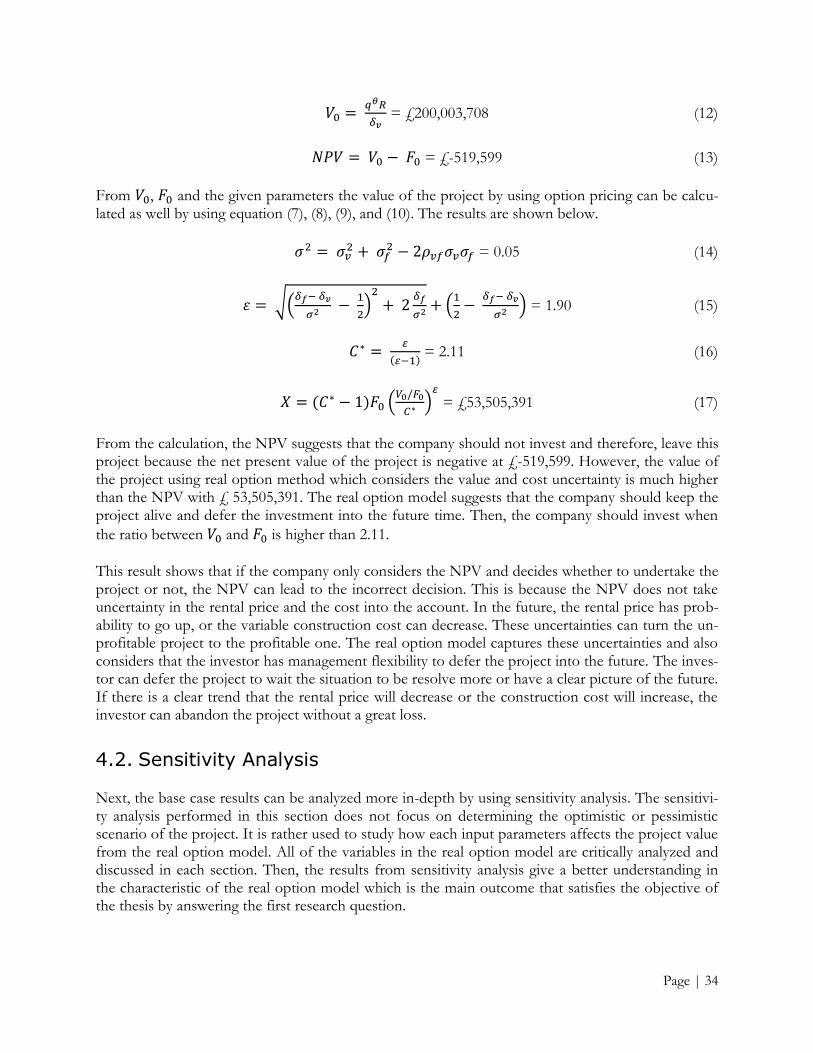
Page | 34

= £200,003,708 (12)

= £-519,599 (13)

From , and the given parameters the value of the project by using option pricing can be calcu-lated as well by using equation (7), (8), (9), and (10). The results are shown below.

= 0.05 (14)

√(

)

(

) = 1.90 (15)

= 2.11 (16)

(

)

= £53,505,391 (17)

From the calculation, the NPV suggests that the company should not invest and therefore, leave this project because the net present value of the project is negative at £-519,599. However, the value of the project using real option method which considers the value and cost uncertainty is much higher than the NPV with £ 53,505,391. The real option model suggests that the company should keep the project alive and defer the investment into the future time. Then, the company should invest when

the ratio between and is higher than 2.11.

This result shows that if the company only considers the NPV and decides whether to undertake the project or not, the NPV can lead to the incorrect decision. This is because the NPV does not take uncertainty in the rental price and the cost into the account. In the future, the rental price has prob-ability to go up, or the variable construction cost can decrease. These uncertainties can turn the un-profitable project to the profitable one. The real option model captures these uncertainties and also considers that the investor has management flexibility to defer the project into the future. The inves-tor can defer the project to wait the situation to be resolve more or have a clear picture of the future. If there is a clear trend that the rental price will decrease or the construction cost will increase, the investor can abandon the project without a great loss.

4.2. Sensitivity Analysis

Next, the base case results can be analyzed more in-depth by using sensitivity analysis. The sensitivi-ty analysis performed in this section does not focus on determining the optimistic or pessimistic scenario of the project. It is rather used to study how each input parameters affects the project value from the real option model. All of the variables in the real option model are critically analyzed and discussed in each section. Then, the results from sensitivity analysis give a better understanding in the characteristic of the real option model which is the main outcome that satisfies the objective of the thesis by answering the first research question.

Page | 35

4.2.1. Feasible and Optimal Investment Value

First, the unit construction cost and unit rental rate can be changed in order to determine the opti-mal value of these to parameters that make the investment to become feasible. The investment is feasible to invest now when the NPV of the project equals to zero. Hence, those two parameters can be determined by the backward calculation. The results are presented in Table 4.2. The table also shows the values of unit construction cost and unit rental rate that make the NPV and real option value to be the same. This is called the optimal investment values which in the other word, the val-

ues that make the ratio between and equals to 2.11, which is the value of .

Parameters NPV Real Option

Unit construction cost sensitivity analysis (fix the unit rental rate at = 250)

Base Case

= 2,000.00 Feasible Case

= 1,993.36 Optimal Case

= 649.99

£-519,599 £0 £105,133,712

£53,505,391 £53,630,825 £105,133,712

0.99 1.00 2.11

Unit rental rate sensitivity analysis (fix the unit construction cost at = 2,000)

Base Case

= 250.00 Feasible Case

= 250.65 Optimal Case

= 528.38

£-519,599 £0 £222,186,874

£53,505,391 £53,770,155 £222,186,874

0.99 1.00 2.11

Table 4.2 Sensitivity Analysis of Unit Construction Cost and Unit Rental Rate

From the analysis, it is obvious that a slight decrease in unit construction cost, from £2,000 per unit to £1,993.36 per unit, and increase in unit rental rate, from £250 per m2 to £250.65 per m2, turn the project to become feasible. This is because the NPV of the base case has a relatively small negative value. Furthermore, this is a very large scale commercial real estate project with 70,000 m2 available space. A minimal change in these parameters results a significant change in the project value.

When considering the optimal value to invest, the unit construction cost has to drop considerably to £649.99, or the unit rental rate has to be as high as £528.38 per m2 in order to make this project be-come optimal to invest now. As discussed above, a slight change in both parameters can turn the project to become favorable or unfavorable one. This means that waiting to invest in the future has the value in itself because waiting can help the owner of the project to resolve the situation and has a better prospect about the future. On account of this, the value of the project now (the NPV) has to be high enough to a certain level to compensate for the risks and uncertainties that might happen in the future. More importantly, it should also be noted that even though £649.99 of unit construction

cost and £528.38 per m2 of unit rental rate make the project to reach the optimal ratio between

and at 2.11, the values of option are not the same. This situation is caused by the degree of uncer-tainty in the cost and the value which is discussed in more details in the next section of sensitivity analysis.

Page | 36

4.2.2. Unit Value and Option Value

After identifying the feasible and the optimal value of unit construction cost ( ) and unit rental rate

( ), these two input parameters can be changed as well in order to examine the effect on the option value. This is done by fixing one parameter and changing another one. The rest of the parameters such as level of uncertainty and expected rate of return are also fixed according to the base parame-ters in the case study. The results of the analysis are displayed in Figure 4.1.

Figure 4.1 Sensitivity Analysis of Unit Value and Option Value

Figure 4.1 shows that the option value falls when the unit construction cost increases. Conversely, the option value rises when the unit rental rate increases. This aligns with an intuition in any invest-ment problems. Anyway, it still should be noted that the effect from increasing the rental value on the option value is substantially higher than the effect from the increase in unit construction cost.

The reason for this is because the unit rental rate is the perpetuity income of the project that the owner of the building will receive forever after finishing the construction. On the other hand, the unit construction cost is the single time cost that the owner has to pay during the construction phase and then once the project is finished, there is no more cost in the project. This is why a slight in-crease in unit rental rate considerably affects the option value.

0 100 200 300 400 500 600 700

0

50

100

150

200

250

300

0 500 1000 1500 2000 2500 3000 3500 4000

Op

tio

n V

alu

e (

Mill

ion

s £)

Unit Construction Cost (K)

Unit Rental Rate (R)

Unit Construction Cost (K)

Unit Rental Rate (R)

Page | 37

4.2.3. Level of Uncertainty and Option Value

Next, the analysis examines the sensitivity of the option value according to the levels of unit con-

struction cost and unit rental rate uncertainty ( and ). As previous, this analysis can be done by

changing the level of uncertainty in one type ( or ) of the time while fixing all of the parameters

as in the base case. The results of this sensitivity analysis are shown in Figure 4.2 below.

Figure 4.2 Sensitivity Analysis of Level of Uncertainty and Option Value

From the results, it can be clearly seen that the level of uncertainty (volatility) affects greatly on the option price and the higher the volatility, the higher the option value is. This is because the volatility is the indicator measuring the possible spread of the unit construction cost and unit rental rate. The higher volatility means that there is a wider range of the possible values. This can be described by Figure 4.3 which shows the spread of possible unit rental rate in different level of uncertainty.

30.00

50.00

70.00

90.00

110.00

130.00

150.00

0% 10% 20% 30% 40% 50% 60% 70% 80% 90% 100%

Option Value (Millions £)

Volatility

Unit Construction Cost Uncertainty (σf)

Unit Rental Rate Uncertainty (σv)

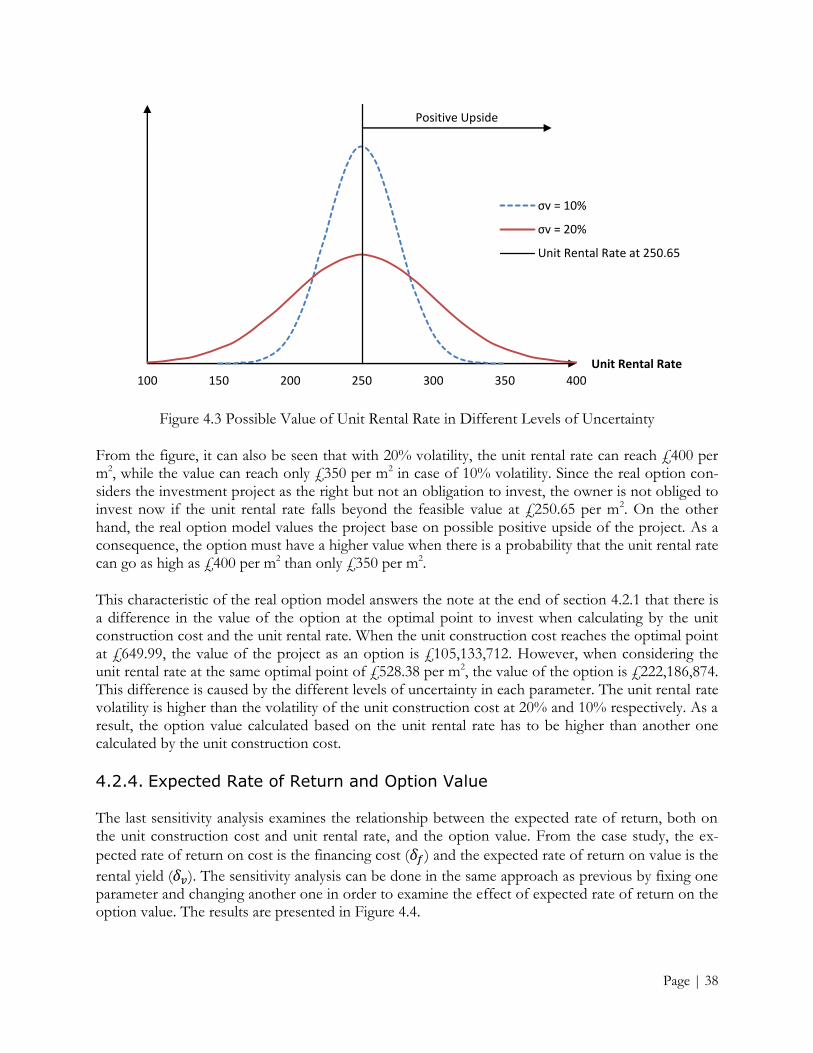
Page | 38

Figure 4.3 Possible Value of Unit Rental Rate in Different Levels of Uncertainty

From the figure, it can also be seen that with 20% volatility, the unit rental rate can reach £400 per m2, while the value can reach only £350 per m2 in case of 10% volatility. Since the real option con-siders the investment project as the right but not an obligation to invest, the owner is not obliged to invest now if the unit rental rate falls beyond the feasible value at £250.65 per m2. On the other hand, the real option model values the project base on possible positive upside of the project. As a consequence, the option must have a higher value when there is a probability that the unit rental rate can go as high as £400 per m2 than only £350 per m2.

This characteristic of the real option model answers the note at the end of section 4.2.1 that there is a difference in the value of the option at the optimal point to invest when calculating by the unit construction cost and the unit rental rate. When the unit construction cost reaches the optimal point at £649.99, the value of the project as an option is £105,133,712. However, when considering the unit rental rate at the same optimal point of £528.38 per m2, the value of the option is £222,186,874. This difference is caused by the different levels of uncertainty in each parameter. The unit rental rate volatility is higher than the volatility of the unit construction cost at 20% and 10% respectively. As a result, the option value calculated based on the unit rental rate has to be higher than another one calculated by the unit construction cost.

4.2.4. Expected Rate of Return and Option Value

The last sensitivity analysis examines the relationship between the expected rate of return, both on the unit construction cost and unit rental rate, and the option value. From the case study, the ex-

pected rate of return on cost is the financing cost ( ) and the expected rate of return on value is the

rental yield ( ). The sensitivity analysis can be done in the same approach as previous by fixing one parameter and changing another one in order to examine the effect of expected rate of return on the option value. The results are presented in Figure 4.4.

0

0.0 02

0.0 04

0.0 06

0.0 08

0.0 1

0.0 12

0.0 14

0.0 16

0.0 18

100 150 200 250 300 350 400

Unit Rental Rate

σv = 10%

σv = 20%

Unit Rental Rate at 250.65

Positive Upside

Page | 39

Figure 4.4 Sensitivity Analysis of Expected Rate of Return and Option Value

From the figure, the analysis starts at the 4.6% expected rate of return from both financing cost and rental yield because the lowest expected rate of return has to be the same as risk free rate, which is 4.6% in this case. As the results, it is apparent that the option value has a positive correlation with financing cost, but exponentially negative correlation with rental yield. The relationship can be ex-plained by the concept of discounted cash flow (DCF). The DCF concept has two basic rules which are the today’s money has more value than the future’s money, and the safer money has more value than the riskier money. With these concepts, it means that the future cash flows from a particular asset have to be discounted back into the present values by the expected rate of return. The higher the expected rate of return means the asset is risker, thus the future cash flows are discounted more and have less value today.

Considering the unit construction cost which is the cash outflow of the project, the real option model considers that the project owner can develop the commercial real estate in the future at

£2,000 per unit. For this, the £2,000 per unit cash outflow in the future has less value today. Increas-ing the financing cost leads to the even lower today’s unit construction cost because the cost is dis-counted more. On the account of this, the construction project costs less and the value of the pro-ject calculated by the real option increases. The same line of reasoning can be applied to the unit rental rate. When the rental yield rises, the future cash inflows from rent are discounted more and have the lower value at present. This results in the decrease in the income and then, the project val-ue. However, increasing the rental yield severely affects the project value because the option value

also depends on the expected project value ( ). The expected project value is calculated according to the equation (12) as a perpetuity income. So, not only does an increase in rental yield affect direct-ly on the real option model, but it also significantly affects the expected value of the project. As a consequence, the option value falls exponentially when the rental yield rises.

0

20

40

60

80

100

120

140

160

4% 6% 8% 10% 12% 14% 16% 18% 20% 22%

Option Value (Millions £)

Expected Rate of Return

Financing Cost (δf)

Rental Yield (δv)

Page | 40

4.2.5. Summary of Sensitivity Analysis

From all of the analysis, the effects from changing different parameters on the option value can be summarized according to Table 4.3 below.

Input Parameters Unit Construction Cost

( )

Unit Rental Rate

( )

Feasible Value £1,993.36 £250.65 Optimal Value £649.99 £528.38 Unit Value* - +

Level of Uncertainty ( )* + +

Expected Rate of Return ( )* + - *Changes in the option value when the input parameters increase

Table 4.3 Summary of the Sensitivity Analysis

As shown in Table 4.3, it is very interesting to see that these characteristics of real option corre-sponds with the financial call option in stock as described by Brealey, Meyers, and Allen, F. (2006, p. 581). To elaborate, an increase in unit rental rate (stock value) and level of uncertainty of unit rental rate (volatility of the stock) have a positive effect in the option price. Inversely, an increase in the unit construction cost (exercise price) negatively affects the option price. In addition, this analysis adds the knowledge of the effect on the option value from the volatility of the unit construction cost (exercise price) which normally does not have in financial call option in stock. Also, the analysis pre-sents the effect on the option value from expected rate of return of unit construction cost (exercise price) and unit rental rate (stock value) which are not covered in financial call option as well. The sensitivity analysis yields an interesting result as discussed in details in the previous parts.

In conclusion, the real option model has many variables as the inputs and the results from sensitivity analyses reveal that the input parameters that relate to the unit rental rate have much greater effect on the option value than the parameters related to the unit construction cost. This suggests that the owner of the project must carefully determine all of the input parameters, especially ones that related to the unit rental rate, so that result in project value from the real option model is reliable. In addi-tion, the company should keep a good track on the fluctuation in unit rental rate since it is the key variable that can lead to a dramatic change in the project value as discussed earlier. These comments show that the real option model has higher complexity in term of usage of the model compared with the traditional NPV approach.

All of these characteristics help financial analysts to have a better understanding of the real option model that captures value and cost uncertainties and know how to use the model correctly with some cautions for any real estate development projects.

Page | 41

5. Monte Carlo Simulation Design

After calculating the base result from the case study and analyzing the real option model in a great detail by using sensitivity analysis in chapter 4, the Monte Carlo simulation is introduced as a study to determine the application of the real option model and the effect on the management decision. There are two simulations needed to be performed as mentioned in the methodology chapter which

are simulation, and NPV and real option value simulation. This chapter focuses on stating the purpose of each simulation and explaining how to construct them in order to insure reliability and validity of the thesis. The information used to build the simulations also comes from the case study of commercial development at Spitalfields, East London (Sing, 2001) as in the previous chapter.

5.1. Simulation

According to the real option model, is the ratio between the total present value of the project

( ) and the total present value of the cost ( ). As the investment rule that was described in section

2.3.3, the company should invest in the project now when equals . With this, is a very important parameter since it tells when the company should invest in the project. Therefore, deter-

mining the expected value of in general case is very useful in decision making process. In order

to find the expected value of , a Monte Carlo simulation is used to generate all possible values of

by changing some input variables randomly. The results from the simulation can be used to de-

rive the expected value of in general case and also allow managers to adjust this parameter ac-cording to their risk behavior. This considers as an application of the real option model. Hence, the objective of the simulation can be defined as follow.

Simulation Objective: to find the expected value and all possible values of

After defining the objective of the simulation, the design of the simulation follows the framework that was discussed in section 2.4.2.


In this case, the model for the investment project means the model used for calculating the which is equation (8), (9), and (10) as presented again below.

(8)

Where √(

)

(

) (9)

(10)

Regarding the interdependence between variables, in this simulation, there is neither time nor varia-

ble interdependence between level of uncertainty in unit construction cost ( ) and unit rental rate

( ), or the expected rate of returns ( and ). This is because these variables do not change ac-

Page | 42

cording to time and also this simulation consider at one point of the time which is at the present

time ( ). For the interdependence between variable, there is no interdependence as well since from

the case, the correlation between rental and construction cost volatility ( ) equals to zero and

there is no correlation between expected rate of return.


The next step is to identify the random variables to be sampled by the simulation. is calculated by

using equation (8), (9), and (10) and from these equations, it can be seen that the value of de-

pends on the levels of uncertainty of unit construction cost ( ), uncertainty of unit rental rate ( ),

and the expected rate of returns ( and ). This simulation focuses on changing the level of uncer-

tainties on only because these two variables are not certain since they are determined from the market study and forecast. While, the expected rate of returns are much more certain input because

the expected rate of return on the rent ( ) and the financing cost ( ) are determined by the com-

pany and the financial institution themselves.

Regarding the probability distributions for these random variables, the key characteristics of the level of uncertainties is that first, the level of uncertainties has the minimum value at 0, while the maxi-mum value cannot exceed 1.The second is that the possible values of these variables are the real number. On account of these, the selected probability distribution has to be a continuous function but it cannot be uniform or normally distributed. This is because the uniform distribution means that there is an equal probability for the random variables to be any values from 0 to 1. For example, there is the equal probability that the level of uncertainty in unit construction cost is 0.01 or 1. This is not correct in this case since the case already estimated the values for both uncertainties which are 0.1 and 0.2 for volatility of unit construction cost and rental volatility respectively. These estimated value can be consider as the averages of the level of uncertainties. On the other hand, the probability distribution of the random variables cannot be the normal distribution because the boundary for the changes of these values do not equal. To elaborate, for the level of uncertainty in unit construction cost which has the estimated (mean) value at 0.1, this means that the value can decrease only for 0.1 while it can increase for 0.9 more. This is the same for the level of uncertainty in unit rental rate. This characteristic causes a right skew to the distribution and hence, the normal distribution does not fit to the random variables.

With all of these reasons, the probability distribution which is a good representative for the random variables is lognormal distribution. The lognormal distribution is a continuous probability distribu-tion of a random variable whose logarithm is normally distributed. This distribution is commonly used in computational finance for non-negative variables (Jäckel, 2002, p. 14-15). It has two control

parameters which are the mean of and the standard deviation of . Due to the lag of in-formation from the case study, these two parameters are derived from the following assumptions.

Assume that mean of equals to , given that

The mean of the level of uncertainty in unit construction cost equals to 0.1

The mean of level of uncertainty in unit rental rate equals to 0.2

The company is certain that the lowest possible of level of uncertainties is 0. This leads to

The values of ±3 standard deviation of the level of uncertainty in unit construction cost are 0 and 0.2.

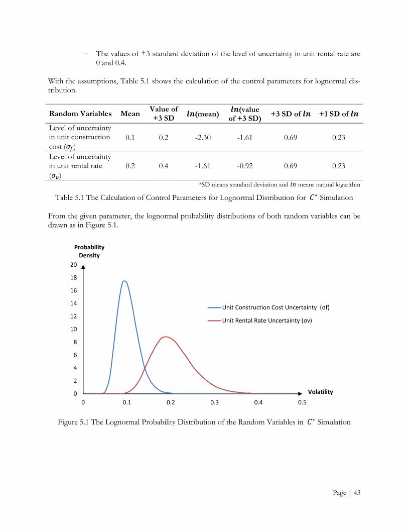
Page | 43

The values of ±3 standard deviation of the level of uncertainty in unit rental rate are 0 and 0.4.

With the assumptions, Table 5.1 shows the calculation of the control parameters for lognormal dis-tribution.

Random Variables Mean Value of +3 SD

(mean) (value

of +3 SD) +3 SD of +1 SD of

Level of uncertainty in unit construction

cost ( ) 0.1 0.2 -2.30 -1.61 0.69 0.23

Level of uncertainty in unit rental rate

( )

0.2 0.4 -1.61 -0.92 0.69 0.23

*SD means standard deviation and means natural logarithm

Table 5.1 The Calculation of Control Parameters for Lognormal Distribution for Simulation

From the given parameter, the lognormal probability distributions of both random variables can be drawn as in Figure 5.1.

Figure 5.1 The Lognormal Probability Distribution of the Random Variables in Simulation

0

2

4

6

8

10

12

14

16

18

20

0 0.1 0.2 0.3 0.4 0.5

Probability Density

Volatility

Unit Construction Cost Uncertainty (σf)

Unit Rental Rate Uncertainty (σv)

Page | 44

Step 3: Simulate random variables, calculate, and collecting results

The procedure of running the simulation can be described by the flow chart in Figure 5.2 with 50,000 iterations. The remaining variables used in the simulation are the same as in the case study in chapter 4. Table 5.2 shows the values of these variables. The results from the simulation are present-ed and discussed in the chapter 6 of the thesis.



Rental yield (%) = 7 Correlation between rental and construction cost volatility = 0.0

Table 5.2 List of the Input Parameters for Simulation

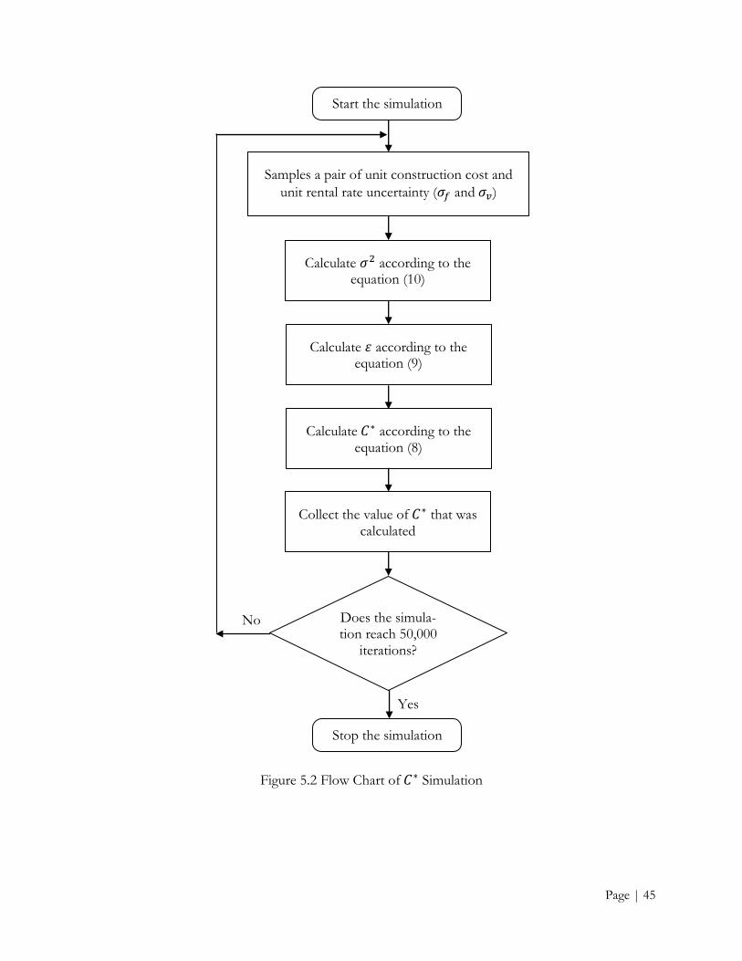
Page | 45

Figure 5.2 Flow Chart of Simulation

Start the simulation

Samples a pair of unit construction cost and

unit rental rate uncertainty (𝜎𝑓 and 𝜎𝑣)

Calculate 𝜎 according to the equation (10)

Calculate 𝜀 according to the equation (9)

Calculate 𝐶 according to the equation (8)

Collect the value of 𝐶 that was calculated

Does the simula-tion reach 50,000

iterations?

Stop the simulation

Yes

No

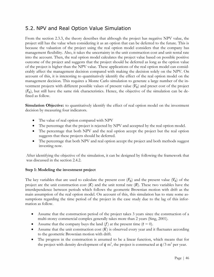
Page | 46

5.2. NPV and Real Option Value Simulation

From the section 2.3.3, the theory describes that although the project has negative NPV value, the project still has the value when considering it as an option that can be deferred to the future. This is because the valuation of the project using the real option model considers that the company has management flexibility. Also, it takes the uncertainty in the unit construction cost and unit rental rate into the account. Then, the real option model calculates the project value based on possible positive outcome of the project and suggests that the project should be deferred as long as the option value of the project is higher than the NPV value. These applications of the real option model can consid-erably affect the management decision compared with making the decision solely on the NPV. On account of this, it is interesting to quantitatively identify the effect of the real option model on the management decision. This requires a Monte Carlo simulation to generate a large number of the in-

vestment projects with different possible values of present value ( ) and preset cost of the project

( ), but still have the same risk characteristics. Hence, the objective of the simulation can be de-fined as follow.

Simulation Objective: to quantitatively identify the effect of real option model on the investment decision by measuring four indicators.

The value of real option compared with NPV

The percentage that the project is rejected by NPV and accepted by the real option model.

The percentage that both NPV and the real option accept the project but the real option suggests that these projects should be deferred.

The percentage that both NPV and real option accept the project and both methods suggest investing now.

After identifying the objective of the simulation, it can be designed by following the framework that was discussed in the section 2.4.2.


The key variables that are used to calculate the present cost ( ) and the present value ( ) of the

project are the unit construction cost ( ) and the unit rental rate ( ). These two variables have the interdependence between periods which follows the geometric Brownian motion with drift as the main assumption of the real option model. On account of this, this simulation has to state some as-sumptions regarding the time period of the project in the case study due to the lag of this infor-mation as follow.

Assume that the construction period of the project takes 3 years since the construction of a multi-storey commercial complex generally takes more than 2 years (Sing, 2001).

Assume that the company buys the land ( ) at the present time ( = 0).

Assume that the unit construction cost ( ) is observed every year and it fluctuates according to the geometric Brownian motion with drift.

The progress in the construction is assumed to be a linear function, which means that for

the project with density development of m2, the project is constructed at /3 m2 per year.

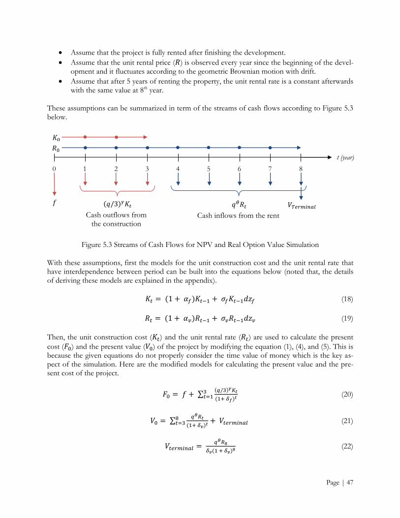
Page | 47

Assume that the project is fully rented after finishing the development.

Assume that the unit rental price ( ) is observed every year since the beginning of the devel-opment and it fluctuates according to the geometric Brownian motion with drift.

Assume that after 5 years of renting the property, the unit rental rate is a constant afterwards with the same value at 8th year.

These assumptions can be summarized in term of the streams of cash flows according to Figure 5.3 below.

Figure 5.3 Streams of Cash Flows for NPV and Real Option Value Simulation

With these assumptions, first the models for the unit construction cost and the unit rental rate that have interdependence between period can be built into the equations below (noted that, the details of deriving these models are explained in the appendix).

(18)

(19)

Then, the unit construction cost ( ) and the unit rental rate ( ) are used to calculate the present

cost ( ) and the present value ( ) of the project by modifying the equation (1), (4), and (5). This is because the given equations do not properly consider the time value of money which is the key as-pect of the simulation. Here are the modified models for calculating the present value and the pre-sent cost of the project.

∑

(20)

∑

(21)

(22)

𝑞 3 𝛾𝐾𝑡 𝑞𝜃𝑅𝑡

t (year)

0 1 2 3 4 5 6 7 8

𝐾

𝑅

𝑓

Cash outflows from the construction

Cash inflows from the rent

𝑉𝑇𝑒𝑟𝑚𝑖𝑛𝑎𝑙

Page | 48

After calculating the project’s present cost ( ) and present value ( ), the NPV and the real option

value ( ) of the project can be found by these equations.

(23)

(

)

(7)

Where

(8)

√(

)

(

) (9)

(10)


Although there are several models in this simulation, there are only two random variables needed to

be sampled by the computer. The random variables are and which are standard Wiener

process (Brownian motion). The probability distributions of and are normal distribution

with zero mean and unit standard deviation (Dixit and Pindyck, 1994, p. 65-66). Figure 5.4 displays

the probability distributions of and .

Figure 5.4 The Normal Probability Distribution of the Random Variables in NPV and Real Option Value Simulation

0

0.05

0.1

0.15

0.2

0.25

0.3

0.35

0.4

0.45

-5 -4 -3 -2 -1 0 1 2 3 4 5

Probability Density

dz

dz(f) and dz(v)

Page | 49

Step 3: Simulate random variables, calculate, and collecting results

The input parameters for the models used in this simulation are shown in Table 5.3. In addition, the procedure in running the simulation is explained in Figure 5.5. The simulation runs for 50,000 itera-tions.


Land cost (£) = 44,000,000 Maximum density of development (m2) = 70,000 Unit construction cost at year 0(£ per m2) = 2,000 Instantaneous drift of unit construction cost (%) = 10

Volatility of unit construction cost (%) = 10


Unit rental rate at year 0(£ per m2) = 250 Instantaneous rental drift (%) = 5 Rental volatility (%) = 20 Rental yield (%) = 7 Correlation between rental and construction cost volatility = 0.0

Cost elasticity of scale = 1.01 Price elasticity of scale = 0.98

Table 5.3 List of the Input Parameters for NPV and Real Option Value Simulation

Page | 50

Figure 5.5 Flow Chart of NPV and Real Option Value Simulation

Sample a pair of standard Wiener process (𝑑𝑧𝑓 and 𝑑𝑧𝑣 )

Stop the simulation

Start the simulation

Does the simulation reach 50,000 itera-

tions?

Is the number of

year higher than 3?

Set the number of year to 1

Is the number of year higher than 8?

Calculate the unit construction cost and the unit rental rate according to the equation (18) and (19)

Calculate the present value ac-cording to the equation (21)

Calculate the present cost ac-cording to the equation (20)

Increase the number of year by 1

Calculate the terminal value (𝑉𝑡𝑒𝑟𝑚𝑖𝑎𝑛𝑙) ac-cording to the equation (22)

Calculate the NPV and the option value according to the equation (23), (7), (8), (9), and (10)

Collect the value of NPV and real option that were calculated

Yes

No

Yes

No

No

Yes

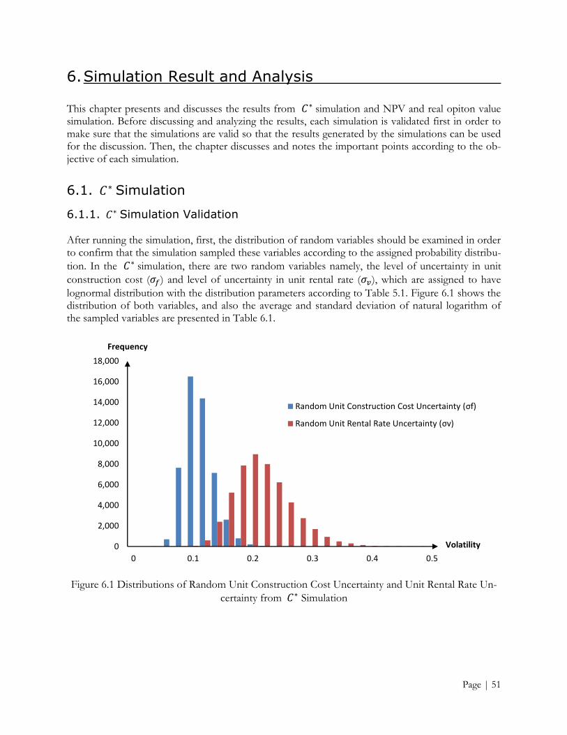
Page | 51

6. Simulation Result and Analysis

This chapter presents and discusses the results from simulation and NPV and real opiton value simulation. Before discussing and analyzing the results, each simulation is validated first in order to make sure that the simulations are valid so that the results generated by the simulations can be used for the discussion. Then, the chapter discusses and notes the important points according to the ob-jective of each simulation.

6.1. Simulation

6.1.1. Simulation Validation

After running the simulation, first, the distribution of random variables should be examined in order to confirm that the simulation sampled these variables according to the assigned probability distribu-

tion. In the simulation, there are two random variables namely, the level of uncertainty in unit

construction cost ( ) and level of uncertainty in unit rental rate ( ), which are assigned to have

lognormal distribution with the distribution parameters according to Table 5.1. Figure 6.1 shows the distribution of both variables, and also the average and standard deviation of natural logarithm of the sampled variables are presented in Table 6.1.

Figure 6.1 Distributions of Random Unit Construction Cost Uncertainty and Unit Rental Rate Un-

certainty from Simulation

0

2,000

4,000

6,000

8,000

10,000

12,000

14,000

16,000

18,000

0 0.1 0.2 0.3 0.4 0.5

Frequency

Volatility

Random Unit Construction Cost Uncertainty (σf)

Random Unit Rental Rate Uncertainty (σv)

Page | 52

Random Variables Mean of SD of

Level of uncertainty in unit construction cost ( ) -2.30 0.23

Level of uncertainty in unit rental rate ( ) -1.61 0.23

Table 6.1 Average and Standard Deviation of Random Unit Construction Cost and Unit Rental Rate

Uncertainty from Simulation

Figure 6.1 confirms that the random variables that were sampled by the simulation follow the lognormal distribution with the given distribution parameters because the result in Figure 6.1 shows that the distributions are very similar to the Figure 5.1. In addition, the average and standard devia-tion of natural logarithm of both random variables have the same values as defined in Table 5.1. This confirms the reliability and validity of the simulation.

6.1.2. Simulation Result and Analysis

Next, possible values of are plotted to examine the distribution of the results and then, the key statistical measurements are calculated for the analysis of the results. Figure 6.2 illustrates the distri-

bution of all possible values of and Table 6.1 presents the statistical results.

Figure 6.2 Distribution of Possible Values of

Statistical Measurement Value

Minimum 1.63 Maximum 4.25 Mean 2.16 Standard Deviation 0.22 Skewness 1.14

Table 6.2 Statistical Measurements of Simulation

0

1,000

2,000

3,000

4,000

5,000

6,000

1.5 1.75 2 2.25 2.5 2.75 3 3.25 3.5 3.75 4 4.25 4.5

Frequency

Value

C*

Page | 53

The histogram and skewness measurement show that the results of from the simulation are not normally distributed. The distribution is right skew as it can be seen from the histogram and the pos-itive skewness measurement. The result is reliable because the random variables, the level of uncer-

tainty in unit construction cost ( ) and level of uncertainty in unit rental rate ( ), which are the

inputs of the simulation are assigned to be lognormal distribution with a right skew.

As mentioned in the theory, is the ratio between the present value ( ) and present cost ( ) and from the investment rule of the real option model, the company should invest in the project now

when the value of / is equal or higher than . If the ratio is less than the value of , the company should defer the investment. From the statistical measurements, the results suggest that

the company should invest in the project now only when the present value ( ) is 2.16 times higher

than the present cost ( ) which is the average value of received form the simulation. This value

is slightly higher than the value of at 2.11 which was calculated in the base case (section 4.1). The

reason for the difference is that the from the base case considered the given level of uncertainties

( and ) to be precisely determined. This is not the case in reality; no company can determine

these values without uncertainty. In conclusion, the result of the at 2.16 can be used as a general decision criteria which suggests that a firm should invest in a real estate project when the value of the project doubles the development cost. This can significantly change how companies decide to invest in a project. With this fact in mind, investing in a project when the value is higher than the cost according to NPV rule is not applicable anymore. The value of the project must be much high-er than the cost, or 2.16 times higher to be precise. This is because the real option method considers that the value of the project can either increase or decrease in the future due to uncertainties, and deferring the investment to receive more information is valuable. So, the present value of the project has to be high enough to compensate for the risk that the value of the project can decrease. This high present value also needs to cover for the company’s right to wait in order to receive more in-formation in the future.

Considering further, the value of at 2.16 is the expected optimal ratio to invest now for a normal investor. However, the company can characterize itself to be more risk taker or risk adverse investor. If the company characterize itself to be a risk taker investor, the company can decide to invest in the

project now when the ratio between and is lower than 2.16. Conversely, the risk adverse com-

pany will invest in the project when the ratio between and is higher than 2.16. The standard

deviation of can be used for adjusting the expected value of according to the risk characteris-tic of the company. For example, if the company has a positive aspect of the unit rental rate, the

company can adjust the to be one standard deviation lower than the expected value. So, the ad-

justed will equal to 1.94. Furthermore, the simulation also tells the company that the can go as high as 4.25 or can be as low as 1.63 which is the extreme case of the project. These results pro-vides the insight of the most optimistic and pessimistic case to the company without any subjective decision as the sensitivity analysis. Moreover, these two values also specify the appropriate range that

can be adjusted according to the risk characteristic of the company.

To sum up, the thesis found that in general case, a company should invest in a real estate project when the value doubles the cost of development. Otherwise, it is better to defer the investment.

Furthermore, the results from the simulation allow the company to properly adjust the value of according to their risk characteristic which is an application of the real option model.

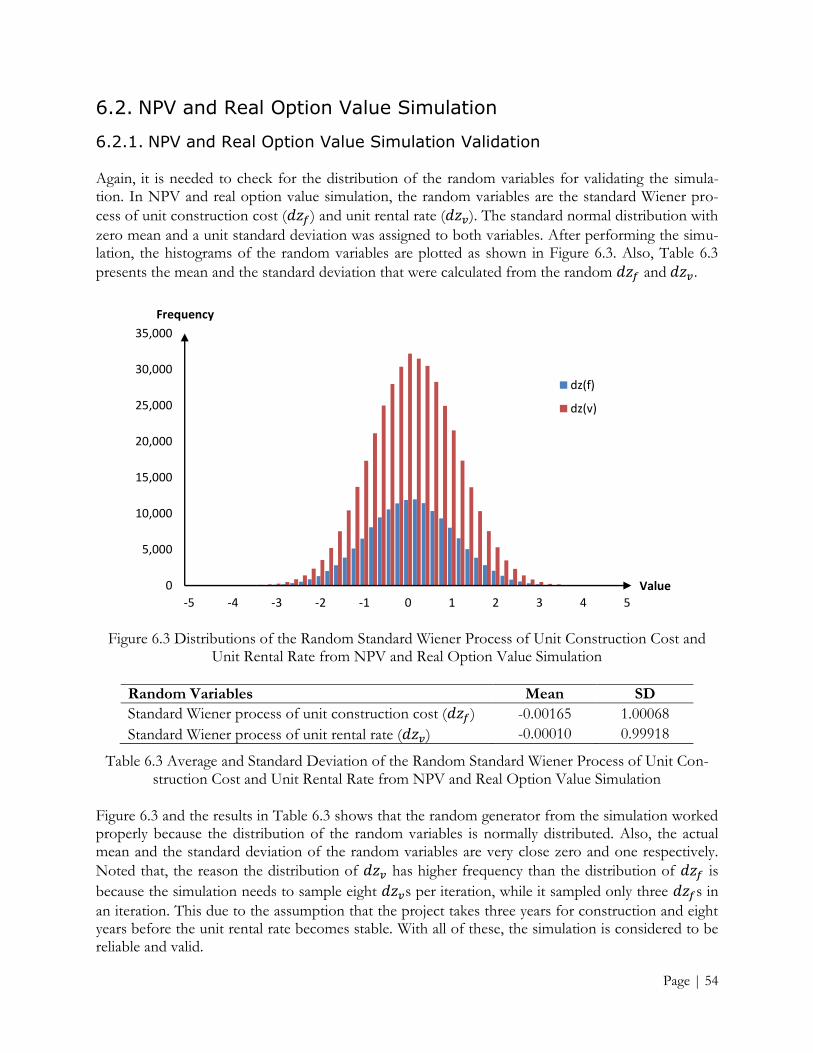
Page | 54

6.2. NPV and Real Option Value Simulation

6.2.1. NPV and Real Option Value Simulation Validation

Again, it is needed to check for the distribution of the random variables for validating the simula-tion. In NPV and real option value simulation, the random variables are the standard Wiener pro-

cess of unit construction cost ( ) and unit rental rate ( ). The standard normal distribution with

zero mean and a unit standard deviation was assigned to both variables. After performing the simu-lation, the histograms of the random variables are plotted as shown in Figure 6.3. Also, Table 6.3

presents the mean and the standard deviation that were calculated from the random and .

Figure 6.3 Distributions of the Random Standard Wiener Process of Unit Construction Cost and Unit Rental Rate from NPV and Real Option Value Simulation

Random Variables Mean SD

Standard Wiener process of unit construction cost ( ) -0.00165 1.00068

Standard Wiener process of unit rental rate ( ) -0.00010 0.99918

Table 6.3 Average and Standard Deviation of the Random Standard Wiener Process of Unit Con-struction Cost and Unit Rental Rate from NPV and Real Option Value Simulation

Figure 6.3 and the results in Table 6.3 shows that the random generator from the simulation worked properly because the distribution of the random variables is normally distributed. Also, the actual mean and the standard deviation of the random variables are very close zero and one respectively.

Noted that, the reason the distribution of has higher frequency than the distribution of is

because the simulation needs to sample eight s per iteration, while it sampled only three s in

an iteration. This due to the assumption that the project takes three years for construction and eight years before the unit rental rate becomes stable. With all of these, the simulation is considered to be reliable and valid.

0

5,000

10,000

15,000

20,000

25,000

30,000

35,000

-5 -4 -3 -2 -1 0 1 2 3 4 5

Frequency

Value

dz(f)

dz(v)

Page | 55

Next, Figure 6.4 and Figure 6.5 illustrate the stochastic process of the unit construction cost ( ) and

the unit rental rate ( ) that were assigned to follow geometric Brownian motion with drift. This is also to prove that the simulation correctly simulates both variables according to the assumption of the real option model.

Figure 6.4 Sample Path of Geometric Brownian Motion with Drift of Unit Construction Cost from NPV and Real Option Value Simulation

Figure 6.5 Sample Path of Geometric Brownian Motion with Drift of Unit Rental Rate from NPV and Real Option Value Simulation

1,000

1,500

2,000

2,500

3,000

3,500

4,000

0 1 2 3

Unit Costruction Cost (£ per m2)

Year (th)

Series1

Series2

Series3

Series4

Series5

0

100

200

300

400

500

600

700

800

0 1 2 3 4 5 6 7 8

Unit Rental Rate (£ per m2)

Year (th)

Series1

Series2

Series3

Series4

Series5

Page | 56

6.2.2. NPV and Real Option Value Simulation Result and Analysis

After validating the simulation, the results from the simulation which are values of NPV and real option from different projects are plotted in Figure 6.6 (noted that, the distributions in Figure 6.6 do not contain all of the results from the simulation because the figure wants to focus on the peak areas and the shape of the distribution. Plotting all of the results will deteriorate this focus). Also, Table 6.4 presents the key statistical measurements of NPV and real option value.

Figure 6.6 Distributions of Possible NPV and Real Option Values

Statistical Measurement NPV Real Option

Minimum £-223,240,916 £483,245 Maximum £1,244,792,054 £1,244,792,054 Mean £35,385,190 £88,552,314 Standard Deviation £125,699,163 £92,121,958 Skewness 1.42 2.61

Table 6.4 Statistical Measurements of NPV and Real Option Simulation

From the illustrations and the values of skewness, it is obvious that the possible NPV and real op-tion value are not normally distributed. Both distributions are right skew since the skewness values are positive. This characteristic of the distributions is caused by the assumption in the fluctuation of

the unit construction cost ( ) and the unit rental rate ( ). The unit construction cost and the unit rental rate are assumed to follow geometric Brownian motion with drift which means that the lowest possible value is limited to zero, while there is no limit of the highest value. As the result, the NPV and real option value which were calculated based on these inputs have lognormal distributions in the same way as the unit construction cost and the unit rental rate.

0

1,000

2,000

3,000

4,000

5,000

6,000

-240 -120 0 120 240 360 480 600

Frequency

Value (Millions £)

NPV

Real Option Value

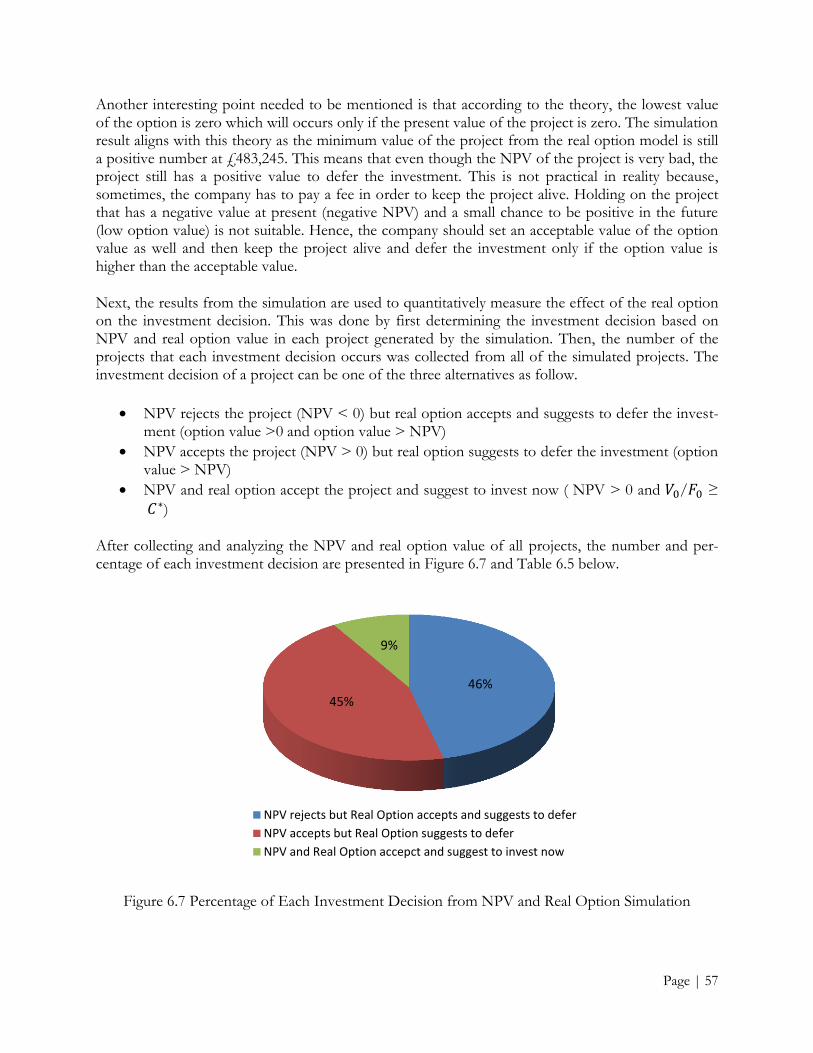
Page | 57

Another interesting point needed to be mentioned is that according to the theory, the lowest value of the option is zero which will occurs only if the present value of the project is zero. The simulation result aligns with this theory as the minimum value of the project from the real option model is still a positive number at £483,245. This means that even though the NPV of the project is very bad, the project still has a positive value to defer the investment. This is not practical in reality because, sometimes, the company has to pay a fee in order to keep the project alive. Holding on the project that has a negative value at present (negative NPV) and a small chance to be positive in the future (low option value) is not suitable. Hence, the company should set an acceptable value of the option value as well and then keep the project alive and defer the investment only if the option value is higher than the acceptable value.

Next, the results from the simulation are used to quantitatively measure the effect of the real option on the investment decision. This was done by first determining the investment decision based on NPV and real option value in each project generated by the simulation. Then, the number of the projects that each investment decision occurs was collected from all of the simulated projects. The investment decision of a project can be one of the three alternatives as follow.

NPV rejects the project (NPV < 0) but real option accepts and suggests to defer the invest-ment (option value >0 and option value > NPV)

NPV accepts the project (NPV > 0) but real option suggests to defer the investment (option value > NPV)

NPV and real option accept the project and suggest to invest now ( NPV > 0 and / ≥

)

After collecting and analyzing the NPV and real option value of all projects, the number and per-centage of each investment decision are presented in Figure 6.7 and Table 6.5 below.

Figure 6.7 Percentage of Each Investment Decision from NPV and Real Option Simulation

46% 45%

9%

NPV rejects but Real Option accepts and suggests to defer

NPV accepts but Real Option suggests to defer

NPV and Real Option accepct and suggest to invest now

Page | 58

Investment Decision Number of Projects Percentage

NPV rejects, but real option accepts and suggests to defer the projects

23,095 46%

NPV accepts the projects but real option suggests to defer the projects

22,599 45%

NPV and real option accept the projects and suggest to invest now

4,306 9%

Total 50,000 100%

Table 6.5 Number of Each Investment Decision from NPV and Real Option Simulation

From the figure, the NPV rejects almost half of the results from the simulation, while the real op-tion suggests that the projects should be deferred. Furthermore, although a large portion of the pro-jects, at 45%, is accepted by NPV, these projects are again should be deferred according to the op-tion value since the option value is still higher than the NPV. Lastly, only 9% or 4,306 projects have the same investment decision from NPV and real option which is to invest in the projects now.

In conclusion, these results quantitatively show that the real option model greatly affects the invest-ment decision by more than 90% at a time when there are cost and value uncertainty in the invest-ment project. This means that making the decision based only on the NPV can lead to a huge error or a wrong timing to invest. Therefore, the traditional way of using only NPV as a decision making tool is not applicable anymore. It is essential for companies to use the real option valuation together with the NPV to evaluate their investment projects. So, they can correctly invest in the projects at the right moment and do not abandon the projects that still have positive aspect in the future.

Page | 59

7. Conclusion

This chapter summarizes all of the findings in relation with the posted research questions. Also, the chapter discusses the knowledge gap that the thesis does not cover and then provides suggestions for the future research.

7.1. Summary of the Findings

According to the introduction part, the thesis posted two research questions which are “What are the main concerns needed to be considered when using real options to evaluate real estate develop-ment projects under uncertainties?” and “How do real options affect investment decision in real es-tate development projects under uncertainties”.

Regarding the first question, the research found out from the study in chapter 4 that the real option model has higher complexity in term of usage compared with traditional NPV approach. When us-ing the real option model, the input parameters should be carefully determined, especially the ones

related to the unit rental rate of the project, which are level of uncertainty ( ) and expected rate of

return ( ). This is because the study found that a slight change in the variables related to the unit rental rate causes a significant change in the real option value. On the contrary, a change in parame-ters related to the unit construction cost has much less effect on the real option value. The thesis also presents the relationship between each input variable and the option value in Table 4.3. The finding provides a better understanding of the mechanism and the logic behind the mathematical formula of the real option model. This helps analysts who want to use the real option to be able to use it more effectively in real estate development evaluation problem.

Next, the thesis answers the second question by the finding from Monte Carlo simulations in chap-

ter 6. First, the study found that the value of which is one of the results from the real option

model plays an important role in the investment decision. This is because indicates that a real

estate development project should be invest now only when the ratio between present value ( ) and

present cost ( ) is higher or equal than the value of . Chapter 6.1 found that in general case, the

value of the is expected to be around 2.16 which means that the value of the project should dou-ble the cost before investing. This totally contradicts with the NPV which suggests that the project should be invested when its value is higher than its cost. On account of this, the real option method greatly affects the traditional decision that is based on the NPV only. Furthermore, the thesis identi-

fies the application of the real option model by showing that a company can adjust the value of

according to its risk behavior. The study found that the value of ranges from 1.63 to 4.25 so that the firm can adjust this value to be lower if it can accept a higher risk, while increases the value of

if the company has a risk adverse behavior.

Regarding another finding, the thesis also quantitatively identifies the effect of the real option on the investment decision in Chapter 6.2. The study found that more than 90% of the time, the real op-tion model changes that investment decision based on the NPV. This is, by 46% of the time, the real option changes the decision from not investing in the project to defer the investment into the fu-ture, and, by 45% of the time, the real option changes the decision from invest in the project now to defer the project. This finding can be concluded that using only NPV to evaluate the investment and

Page | 60

making the decision based on that leads to a huge error. Implementing the real option valuation method can improve the decision making process for companies in real estate development industry. This finding can be supported by the empirical studies from Quigg (1993), and Sing and Patel (2001). The studies statistically present that using real option in real estate development projects is better than the NPV in real estate development investment.

7.2. Academic Significance

First, the thesis contributes to the knowledge in the area of corporate finance by showing how to use the real option model developed by McDonald and Siegel (1986) in real estate development in-vestment. Furthermore, the result from the sensitivity analysis does not restrict only in the real estate development context. When using in other types of investment, the relationship between each input variable and the option value is still the same, but the degree of the effect from each input variable might change only. All of these can be used as a guideline to implement the real option model to evaluate other types of investment in other industries.

Another academic significance of this thesis is that it clearly explains the method to construct a Monte Carlo simulation in investment evaluation problem. Other research papers can follow the framework explained in the thesis and use the explanation in Chapter 5 as the examples for a better understanding when constructing a Monte Carlo simulation. This has academic benefits since most of the textbooks regarding Monte Carlo simulation in finance are highly theoretical. The thesis al-ready simplified these concepts so that they are easier to understand and to be used practically.

Finally, the thesis enriches the knowledge on the real options approach and adds the quantitative findings that show how the real option model affects management decision. In this endeavor, it can raise awareness in the existing alternative approach for investment evaluation instead of the well-known NPV method.

7.3. Suggestions for the Future Research

This study mentioned that there are many variables used in the real option model and it is important to carefully determine these parameters since they have a significant effect on the reliability of the result. However, the thesis does not study on how to collect or determine these data which is one knowledge gap that can be filled by other researches.

Furthermore, due to the complexity of the real option model, the future research can extend the cur-rent study by conducting a qualitative research in order to see the opinions from the real estate de-velopment industry. This can gain an insight on the practical aspect of the real option method and determine other important issues on using the real option for evaluating the investment.

This thesis commented on completeness of the data from the case study which is one of the weak-nesses of the research. The case study still lacks the qualitative information that is necessary for con-structing the Monte Carlo simulations. One suggestion for the future research is to repeat the study by using the same option model and the structure of this study with better rich data. So, the results of the new study will have higher credibility than the current one.

Page | 61

As highlighted in Chapter 6.2, one important thing of the real option model is that the value of the option will still have some small positive value although an investment project has a very bad nega-tive NPV. The thesis pointed out that sometimes it is not practical to defer the project with this val-uation result but the thesis does not address this issue since it is out of the scope of the study. On account of this, the future study can be performed to solve this problem by conducting a study to identify what is the appropriate minimum value of real option that it is still applicable to defer the investment. Alternatively, the future research can conduct a study that modifies the real option model used in this thesis in order to address the issue.

Lastly, the thesis focuses only one type of real option which is the option to defer. However, there might have other types of real option incorporated in real estate development investment such as the option to expand or abandon the project in the future. Another suggestion for the future re-search is to include other types of real option when evaluating a real estate project. On the other hand, the future research can use the concept of deferred option and the model in other contexts outside real estate development investment such as investments in new product development and manufacturing.

Page | 62

References

Armstrong, M., Galli, A., Bailey, W. and Couët, B. (2004) Incorporating technical uncertainty in real option valuation of oil projects, Journal of Petroleum Science and Engineering, Volume 44, Issues 1–2, 31 October, Pages 67-82.

Brealey, R.A., Meyers, S.C. and Allen, F. (2006) Principles of Corporate Finance, 8th edition, New York: McGraw-Hill/Irwin.

Brach, M.A. (2003) Real Options in Practice, New Jersey: John Wiley & Sons, Inc.

Bulan, L., Mayer, C. and Somerville, C.T. (2009) Irreversible investment, real options, and competi-tion: Evidence from real estate development, Journal of Urban Economics, Volume 65, Issue 3, May, Pages 237-251.

Cassimon, D., De Backer,M., Engelen, P.J., Van Wouwe, M. and Yordanov, V. (2011) Incorporat-ing technical risk in compound real option models to value a pharmaceutical R&D licensing opportunity, Research Policy, Volume 40, Issue 9, November, Pages 1200-1216.

Capozza, D. and Sick, G. (1992) Risk and return in land markets, working paper, University of British Columbia, Vancouver.

Collis, J. and Hussey, R. (2009) Business Research: A Practical Guide for Undergraduate and Postgraduate Stu-dents, third edition, New York: Palgrave Macmillan.

Cortazar, G. and Schwartz, E.S. (1997) Implementing a real option model for valuing an undevel-oped oil field, International Transactions in Operational Research, Volume 4, Issue 2, March, Pages 125-137.

Dias, M. (2004) Valuation of exploration and production assets: an overview of real options models, Journal of Petroleum Science and Engineering, Volume 44, Issues 1–2, 31 October, Pages 93-114.

Dixit, A.K. and Pindyck, R.S. (1994) Investment under Uncertainty, Princeton, NJ: Princeton Univ. Press.

Donovan, G.H. and Butry D.T. (2011) The effect of urban trees on the rental price of single-family homes in Portland, Oregon, Urban Forestry and Urban Greening, Volume 10, Issue 3 Pages 163-168.

Duku-Kaakyire, A. and Nanang, D.M. (2004) Application of real options theory to forestry invest-ment analysis, Forest Policy and Economics, Volume 6, Issue 6, October, Pages 539-552.

Fan, Y. and Zhu, L. (2010) A real options base model and its application to China's overseas oil in-vestment decisions, Energy Economics, Volume 32, Issue 3, May, Pages 627-637.

Page | 63

French, N. And Gabrielli, L. (2004) The uncertainty of valuation, Journal of Property Investment and Fi-nance, Volume 22, Issue 6, Pages 484 - 500.

Geltner, D.M., Miller,N.G., Clayton, J. and Eichholtz, P. (2006) Commercial Real Estate Analysis and Investments, Second Edition, California: Thomson Higher Education.

Gimpelevich, D. (2011) Simulation-based excess return model for real estate development: A practi-cal Monte Carlo simulation-based method for quantitative risk management and project valua-tion for real estate development projects illustrated with a high-rise office development case study, Journal of Property Investment and Finance, Volume 29, Issue 2, Pages 115-144.

Graaskamp, J (1972) A rational approach to feasibility analysis, The Appraisal Journal, October, Pages 513-521.

Hertz, D.B. (1968) Investment Policies that Pay Off, Harvard Business Review 46, January–February, Pages 96–108.

Hoesli, M., Jani, E. and Bender, A. (2006) Monte Carlo simulations for real estate valuation, Journal of Property Investment and Finance, Volume 24, Issue 2, Pages 102-122.

Hott, C. (2011) Lending behavior and real estate prices, Journal of Banking and Finance, Volume 35, Issue 9, September, Pages 2429-2442.

Jäckel, P. (2002) Monte Carlo Methods in Finance, West Sussex: John Wiley & Sons Ltd.

Johnson, K. (1985), Risk analysis and project selection: a review of practical issues, ADB Economics Staff Paper, Number 28, ADB, Manila.

Kallio, M., Kuula, M. and Oinonen, S. (2012) Real options valuation of forest plantation investments in Brazil, European Journal of Operational Research, Volume 217, Issue 2, 1 March, Pages 428-438.

Linjie, C. (2010) Research on the risk identification and evaluation of real estate development, Infor-mation Science and Engineering (ICISE), 2010 2nd International Conference, December, Pages 3087-3090.

Loizou, P. and French, N. (2012) Risk and uncertainty in development: A critical evaluation of using the Monte Carlo simulation method as a decision tool in real estate development projects, Jour-nal of Property Investment and Finance, Volume 30, Issue 2, Pages 198-210.

Lucius, D.I. (2001) Real options in real estate development, Journal of Property Investment and Finance, Volume 19 Issue 1, Pages 73 - 78.

Mao, Y. and Wu, W. (2011) Fuzzy Real Option Evaluation of Real Estate Project Base on Risk Analysis, Systems Engineering Procedia, Volume 1, Pages 228-235.

Marco, L. (2008) Determinants of New York City Residential Rental Prices, Michigan journal of busi-ness, Volume 1, Issue 1, Page 61.

Page | 64

McDonald, R. and Siegel, D. (1986) The Value of Waiting to Invest , The Quarterly Journal of Econom-ics, Volume 101, No. 4, November, Pages 707-728.

Meyers, S.C. (1977) Determinants of corporate borrowing, Journal of Financial Economics, Volume 5, Issue 2, November, Pages 147-175.

Miles, M., Berens, L., Eppli, M. and Weiss, M. (2007) Real Estate Development: Principles and Process, 4th edition, Washington, D.C.: Urban Land Institution.

Paddock, J., Siegel, D., Smith, J. (1988) Option Valuation of Claims on Real Assets: The Case of Offshore Petroleum Leases, The Quarterly Journal of Economics, Volume 103, Issue 3, August, Pag-es 479-508.

Pindyck, R.S. (1993) Investments of uncertain cost, Journal of Financial Economics, Volume 34, Issue 1, August, Pages 53-76.

Quigg, L. (1993) Empirical Testing of Real Option-Pricing Models, The Journal of Finance, Volume 48, Issue 2, January, Pages 621-640.

Rocha, K., Salles, L., Garcia, F., Sardinha, J.A., and Teixeira, J.P. (2007) Real estate and real options — A case study, Emerging Markets Review, Volume 8, Issue 1, March, Pages 67-79.

Reutlinger, S. (1970), Techniques for project appraisal under uncertainty, World Bank Occasional Pa-pers, Number 10, Johns Hopkins, Baltimore, MD.

Sing, T.F. (2001) Optimal timing of a real estate development under uncertainty, Journal of Property Investment and Finance, Volume 19, Issue 1, Pages 35-52.

Sing, T.F., Patel, K. (2001) "Empirical evaluation of the value of waiting to invest", Journal of Property Investment and Finance, Volume 19 Issue 6, Pages 535 - 553.

Sun, Y., Huang, R. , Chen, D. and Li, H. (2008) Fuzzy Set-Base Risk Evaluation Model for Real Es-tate Projects, Tsinghua Science and Technology, Volume 13, Supplement 1, October, Pages 158-164.

Titman, S. (1985) Urban Land Prices Under Uncertainty, The American Economic Review, Volume 75, Issue 3, June, Pages 505-514.

Trigeorgis, L. (2011) Real Options and Investment under Uncertainty: Classical Reading and Recent Contribu-tions, Massachusetts: MIT Press.

Wang, S., Yang, Z. and Liu, H. (2011) Impact of urban economic openness on real estate prices: Ev-idence from thirty-five cities in China, China Economic Review, Volume 22, Issue 1, March, Pages 42-54.

Wiley, J., Benefield, J. and Johnson, K. (2010) Green Design and the Market for Commercial Office Space, The Journal of Real Estate Finance and Economics, Volume 41, Issue 2, August, Pages 228-243.

Page | 65

Williams, J. (1991) Real Estate Development as an Option, Journal of Real Estate Finance and Economics, Volume 4, Issue 2, Pages 191-208.

Wu, L.C. and Ong, C.S. (2008) Management of information technology investment: A framework base on a Real Options and Mean–Variance theory perspective, Technovation, Volume 28, Issue 3, March, Pages 122-134.

Page | 66

Appendix

Appendix A: Model of Unit Construction Cost and Unit Rental Rate

According to the assumption that the unit construction cost ( ) and unit rental rate ( ) are ob-served every year and they fluctuate according to the geometric Brownian motion with drift. So, the value of unit construction cost and unit rental rate in each year can be model as follow.

(1a)

(1b)

and follow geometric Brownian motion with drift. So, both variables can be calculated by using equation (6a) and (6b).

(2a)

(2b)

Since both values are observed every year, equals to 1. Substituting this value and rearrange the equations as follow.

(3a)

(3b)

Replacing equations (3a) and (3b) in (1a) and (1b).

(4a)

(4b)

Then, rearranging the both equations yields the models used in the simulation.

(5a)

(5b)


Documents

Real Options in Real Estate Development Investment535523/FULLTEXT01.pdf · Real Options in Real Estate Development Investment Warut Sattarnusart Master of Science Thesis INDEK 2012:66