Real Option Pricing in a Fuzzy Stochastic Environment

I-ming Jiang∗, Po-yuan Chen

∗∗, Chingliang Chang

∗∗∗

Abstract

This paper presents a fuzzy stochastic model for pricing the option to invest in an

irreversible investment. The model considers both randomness and fuzziness in the

value of the investment. Randomness states that the future value is always uncertain,

and fuzziness states that the investor has his own subjective judgments on the system,

which cannot be homogeneous and should be considered. Fuzziness is given by

triangular fuzzy numbers, which are easily applied to the original stochastic model,

McDonald and Siegel (1986). An optimality equation for the range of investment

threshold is derived. It is shown that the optimal price range of the option to invest is

the solution of Bellman equation by dynamic programming. The fuzzy goal is also

presented for the permissible range of the investor’s demand profits, which are

discussed in numerical examples.

Keywords: Real Option, Fuzzy Stochastic Environment, Investor Subjective Judgment,

Optimal Price Range

∗ Corresponding Author: I-ming Jiang, Assistant Professor, Department of Finance, Yuan Ze University,

No. 135, Far-East Rd., Chung-Li, Taoyuan, Taiwan, R.O.C. Email: jiangfinance@saturn.yzu.edu.tw ∗∗

Doctoral Candidate Student at Graduate Institute of Management Sciences, Tamkang University,

Taipei, Taiwan. He also serves as lecturer at department of Public Finance, Jinwen University of Science

and Technology, 99, An-Chung Rd, Hsin-Tien City, Taipei, Taiwan. Email: mikecpy@ms7.hinet.net ∗∗∗

Ph.D. Student in Finance, Graduate School of Management, Yuan Ze University, No. 135, Far-East Rd.,

Chung-Li, Taoyuan, Taiwan, R.O.C. Email: s989409@mail.yzu.edu.tw

1

1. Introduction

The option to invest in an irreversible investment has been valued by the

continuous-time stochastic model of McDonald and Siegel (MS) (1986). Most

investors make and sometimes revise their investment decisions continuously through

time. Thus, the analysis of investment decisions should be devoted to the

continuous-time problems. A stochastic process views the investment’s future value

as a variable that evolves over time, denoting that it is always uncertain. The

irreversible investment is an investment that we cannot recover its initial expenditures

all in case of the market conditions turn out to be worse than anticipated. The

irreversible investment expenditure undermines the classical net present value rule

due to the reason that when the investment is irreversible, the decision to invest can be

postponed when the value of the investment does not exceed the investment threshold

(Pindyck, 1991). The option to invest describes the option-nature of the investment.

When investors make irreversible investment expenditures, they exercise their options

to invest while give up the rights to wait for new information that might affect the

timing of the investment. Viewed from the above perspectives, investment decisions

share three important determinants such as the timing of the investment, irreversibility,

and uncertainty in varying degrees. McDonald and Siegel (1986) contribute to

recognize the important quantitative implications of interaction between the timing of

2

the investment, irreversibility, and uncertainty.

In the MS model, the investment decisions are assumed to be made by

homogeneous investors. This assumption implies that all investors have homogeneous

judgments (homogeneity). Although Brennan (1979) and Stapleton and

Subrahmanyam (1984) have pointed out that the assumption of investors with

homogeneity is the basic economic paradigm, we still argue that there exist the

heterogeneous judgments (heterogeneity) inherent with the investors to affect their

investment decisions. De Bondt (1993), and Mankiw and Zeldes (1991) find empirical

evidence of heterogeneity. One of the ways to describe heterogeneity is to regard the

investors to be optimistic or pessimistic.

The optimism is similar to the idea of the overconfidence of Daniel, Hirshfeiler

and Subrahmanyam (2001). The overconfident (optimistic) investors usually

underestimate the uncertainty degree of the investment, leading to underestimate the

investment threshold. In other words, the optimistic investors easily underestimate the

trigger of the investment and make their decisions to invest. In the context of the

fuzzy theory, the optimism is directly related to the lower membership degree (Peters,

2003). On the other hand, the pessimistic investors are especially likely to

overestimate the threshold and defer the investment decisions. In terms of the theory

of fuzzy sets, the pessimism is directly related to the higher membership degree

3

(Peters, 1996). Hence, the pessimistic and optimistic investors have heterogeneous

references of the membership degree in the fuzzy set, and then their investment

decisions are affected.

The above ideas of the optimism and pessimism allow us to explain the relation

of the uncertainty to the investment. The pessimistic investors are likely to defer the

investment in case that the uncertainty is highly unpredictable because they scare the

failure of the investment. As a result of the pessimism, the uncertainty should be

negatively related to the investment. Some authors, Caballero (1991), Leahy and

Whited (1996), and Pindyck (1991), find that there exists the negative relationship

between uncertainty and investment. In contrast to the pessimistic investors, the

optimistic investors are likely to make the decision-makings to invest because they

usually underestimate the high uncertainty, and look at the investment’s success. As a

result, there should be the positive relation of the uncertainty to the investment for the

optimistic investors. Sarkar (2000, 2003) theoretically derives that the positive

relationship between uncertainty and investment. The derivation can help explain why

some investors invest more than others under uncertainty.

Basak (2000), Detemple and Murthy (1994), Harris and Raviv (1993), Mayshar

(1983), Robinstein (1973), and Shefrin and Statman (1994) have treated heterogeneity

for option pricing. One of the methods applied by the above authors is to treat

4

heterogeneity by the fuzzy theory. Recently, Benninga and Mayshar (1997), and

Robinstein (1994) begin to focus their attention on heterogeneity in pricing option.

However, because the MS model is based on the basic economic paradigm, it has

limited success in explaining the heterogeneity in the investment decision. Thus, there

is a need to modify the MS model.

To the best of our knowledge, this paper first develops the fuzzy stochastic

valuation model of the option to invest. In this model, we add the heterogeneity into

the MS model. The heterogeneity is modeled by the membership degree of the

triangular fuzzy function. We apply the technique of dynamic programming to derive

closed-form solutions (Adda and Cooper, 2003; Dixit and Pindyck, 1994; Peskir and

Shiryaev, 2006), and conduct a comparative-static analysis showing that the range of

the values of the option to invest are sensitive to the investors’ subjective judgments

on the volatilities of both the value of the investment and the investment cost.

In the next section, we first construct a simple case, in which the value of the

investment evolves according to the geometric Brownian motion, but the investment

cost is known and fixed. We solve the optimal investment threshold by dynamic

programming. In Section 3, we apply the fuzzy stochastic process to the simple case

to define a closed interval of the value of the option to invest. And we extend the

fuzzy stochastic process into the MS model. In Section 4, we approximate the fuzzy

5

values of the option to invest in a numerical example and compute fuzzy goal. Finally,

in Section 5, we give concluding remarks.

2. Simple Case

Consider an investor that is trying to invest in a firm or industry specific

investment. The investment is completely irreversible the investor cannot

“uninvest” and recover the investment expenditure. The investment problem is to

decide when it is optimal to undertake the investment. We assume that the investment

cost, I , is known and fixed, but the value of the investment, tV , follows a geometric

Brownian motion of the form,

t V t V t VdV µ V dt σ V dz= + , (1)

where 0Vµ ≥ is the instantaneous expected rates of the returns, 0Vσ ≥ is the

instantaneous standard deviation, and Vdz is the increment of a Wiener process.

Equation (1) implies that the current value of the investment is known, but the future

values evolve according to the lognormal distribution with a variance that grows

linearly with time horizon. Thus, although information arrives over time (the firm

observes V changing), the future value of the investment is always uncertain.

We will be mostly concerned with the ways in which the investment decision is

affected by the uncertainty. Thus, we focus attention on the case with uncertainty, that

6

is, Vσ in equation (1) is greater than zero. The investment problem is to determine

the point at which it is optimal to make an irreversible investment expenditure I in

return for an investment whose value is tV . Since tV evolves stochastically, we will

be unable to determine an investment timing. Thus, our investment rule will base on

the optimal investment threshold *V such that it is optimal to invest once *

tV V≥ .

Then, the investors receive the net payoff *V I− from investing. As we will see, a

higher value of Vσ will result in a higher value *V . When the optimal investment

threshold is higher, fewer investments can exceed the threshold as an implication of

waiting for the investment. Thus, higher uncertainty Vσ can create a greater value to

waiting and thereby affect the investment timing. Following we introduce some

Propositions, which enable us to solve the value of the option to invest using the

dynamic programming.

Proposition 1: Let ( )S tF V denote the value of the option to invest at time t in the

simple case. When *

tV V≥ , stopping is optimal because the value of option to invest

yields no cash flows up to the time T , the only return from holding the option to

invest is its capital appreciation. Hence, in the case where *

tV V< (values of

tV for

which it is not optimal to invest) the Bellman equation (Malliaris and Brock, 1982) is

( )tρFdt E dF= , (2)

where tE denotes the expectation at time t and ρ denotes a discount rate.

Equation (2) indicates that over a time interval dt , the total expected return on the

7

value of the option to invest, ρFdt , is equal to its expected increment value,

( )tE dF .

Proposition 2: If we try the function ( ) 1

S

β

t tF V AV= , then the optimal investment

threshold *V , 1β and ( )S tF V at time t , can now be solved after imposing the

appropriate boundary conditions including the initial, value-matching, and

smooth-pasting conditions. The solutions can be written as follows:

* 1

1 1

βV I

β=

−, (3)

2

1 2 2 2

1 12 1

2 2V V

V V V

µ µ ρβ

σ σ σ

= − + − + >

, (4)

( )

( )( )

1

1

11

*1

1 1 1

1 1

1

βββ

A I Vβ β β

− −− −

= = −

, (5)

and

1

* *

S **

1

, for ,

( ) 1, for .

1

t

β

t tt

V I V V

F V VI V V

β V

− ≥

= < −

(6)

Proof: See Appendix.

Equation (3) gives the solution of the optimal investment threshold *V , and has

the important point that since 1 1β > , we have ( )1 1 1 1β β − > , and this shows that the

optimal investment threshold is greater than the NPV’s threshold, that is, *V I> .

Thus, uncertainty and irreversibility drive a wedge between the optimal investment

threshold *V and I . The size of the wedge is the factor ( )1 1 1β β − . Equation (4)

shows two important implications. First, as Vσ increases, 1β decreases, and

8

therefore ( )1 1 1β β − increases. The greater is the amount of the uncertainty over the

future values of V , the larger is the wedge between *V and I , that is, the larger is

the excess return the investor will demand before it is willing to make the irreversible

investment. Second, as r increases, 1β decreases, so a higher r implies a larger

wedge. Some results concerning 1β are also informative. As σ → ∞ , we have

1 1β → and *V → ∞ , that is, the investor never invest if σ is infinite. Equation (5)

gives the value of the constant A , which is sensitive to 1β and *V . Equation (6)

indicates the binary optimal investment rule. If *V V≥ , it is optimal to invest, and

( )F V is equal to the net payoff *V I− . The most import point is that since 1 1β > ,

we have ( )1 1 1 1β β − > and *V I> . Thus, the value of ( )S tF V is greater than zero.

If *V V< , the investor should wait rather than invest now, and growth in V at some

future times will create a value to waiting, and increase the value of the option to

invest. The solution enables us to further develop the fuzzy values of the option to

invest in the next section.

3. Fuzzy Theory and Fuzzy Values of the Option to Invest

3.1 Fuzzy Theory

By adopting Yoshida (2003), we construct a model where the investment value

process 0

T

t tV

= takes fuzzy values, and then represent the investors’ subjective

9

judgments using the membership degrees of the fuzzy values. For the sake of

simplicity, the membership degrees are given by triangular fuzzy numbers. A fuzzy

number is commonly defined by its corresponding membership function [ ]: 0, 1R γ →

where R denotes all real numbers.

Assumption 1: Let 0

T

t tα

= be an tM -adapted stochastic process such that

( ) ( )0 tα ω V ω< ≤ for all ω∈Ω . Then we represent a fuzzy stochastic process of

the investment value 0 Tt tV = by the following fuzzy random variables:

( )( ) ( )( ) ( )( ):t t tV ω x L x V ω α ω= − , (7)

for t ∈T , ω∈Ω and x ∈R , where ( ) : max 1 , x>0L x x= − ( )x∈R is the

triangular-type shape function (Figure 1).

γ

1

0.8

0.6 ( )( )tV ω x

0.4

0.2 ( )tα ω−

( )tα ω+

x

( ) ( )t tV ω α ω−− ( )tV ω ( ) ( )t tV ω α ω+

+

Figure 1. Fuzzy random variable ( )( )tV ω x

Assumption 2: ( )tα ω is a spread of triangular fuzzy numbers ( )tV ω and

corresponds to the amount of fuzziness in the process. Then the γ -cuts of equation (7)

are closed intervals

10

, ( ) ( ) (1 ) ( ), ( ) (1 ) ( )t γ t t t tV ω V ω γ α ω V ω γ α ω− + = − − + − , ω∈Ω , (8)

and so we write the closed intervals by ( ) ( ) ( ), ( ) : 1t γ t tV ω V ω γ α ω±= ± − for ω∈Ω ,

t ∈T and [ ]0, 1γ∈ .

Now we introduce the Assumption 3 from which we are able to simplify the

formulas of Equation (8).

Assumption 3. The stochastic process ( )α ω± is specified by ( ) ( )t tα ω c V ω± ±= ,

0, 1, 2,..., , t T ω= ∈Ω , where c±

is constant satisfying 0 1c±< < .

( ) ( )t tV ω α ω++

( ) ( )t tV ω α ω−−

Figure 2. The stochastic process ( )α ω±

Assumption 3 is reasonable since ( )α ω measures a size of fuzziness and it

should depend on the volatility σ and the investment value ( )tV ω . But, in reality it

is very difficult to estimate the volatility (Ross, 1999) (Figure 2). To overcome the

difficulty, we use c±

to represent the fuzziness of σ , which can be called as a fuzzy

factor of the process. The fuzzy factor c represents the investor’s subjective

estimation of σ , while α represents the investor’s subjective estimation of the value

of the investment. Substituting ( ) ( )t tα ω c V ω± ±= , where 0 1c c+ −< ≤ < , into

, ( )t γV ω+

, ( )t γV ω−

, ( )t γV ω

( )tV ω

x

t

11

equation (8) gives

( ), ( ) 1 (1 ) ( )t γ tV ω γ c V ω± ±= ± − . (9)

In brief, the fuzzy theory has great contribution in modeling the investors’

heterogeneous judgments on the uncertainty because it can provide a range of

heterogeneous fuzzy values to describe the set of subjective judgments without clear

boundaries. The fuzzy logic performs well because the economic conditions change

quickly and the investors always have their own judgments which are likely to be

quite different from the others. In the next section, we introduce a fuzzified version of

the values of the option to invest.

3.2 Fuzzy Values of the Option to Invest

Let us look at equation (9), because we assume the existence of heterogeneous

judgments, the values of the investment cannot be just single. Hence, they should be a

value range. Following we introduce Propositions to propose a closed-form solution

for the fuzzy values of the option to invest.

Proposition 3: Let the fuzzy stochastic process of the Bellman equation be

( )ρF dt E dF± ±= , and the fuzzy values of the option to invest is ( ) ( ) 1±S

β

t tF V A V±= ,

which must satisfy the initial, value-matching, and smooth-pasting boundary

conditions. Then, we can find the two unknownsthe constant A± , and the fuzzy

12

optimal investment threshold *V

± .

( )( )

* 1

1 1 1

βV I

β γ c

±

±=

− ± − . (10)

and

( )( )

( )1( 1)

*

1

1 1 βγ cA V

β

±− −

± ±± −

= . (11)

We will determine ( )±S tF V in much the same way that we do in Proposition 2.

We concentrate on the case where continuation is optimal for t

V V∗±< , and stopping

is optimal for t

V V∗±≥ . Then, we find the following solution for ( )±

S tF V :

( ) ( )( )( )( )

1

* *

±S *

*

1

, if ,

1 1, if .

1 1

t

βt t

t

V I V V

γ cF V VI V V

Vβ γ c

± ±

±

±

±±

− ≥ ± −= < − ± −

(12)

Proof: See Appendix.

Let us compare equation (3) with equation (10), we assume that the future values

of the investment are random, and there exists the heterogeneous judgments on the

uncertainty. Hence, the value is suitable to be fuzzified. This makes the reasonable

results for the formula of the optimal investment threshold should be a range of the

values not just a single value anymore. To propose the upper and lower bounds to

describe the heterogeneity is the one of the major contributions in our paper. Using

the value bound to describe the threshold is due to the reason that the values of the

investment are always uncertain. We assume that the optima investment rule depends

on whether the values of the investment t

V exceed the optimal threshold *V . Hence,

13

the threshold also has the uncertain nature about its actual value. Equation (10) shows

that *V under the stochastic simple case is replaced with *

V± under the fuzzy

stochastic model. The “ ± ” for the equations comes from the fuzzy random variables

gives the closed-form of the optimal investment threshold, and has the important point

that since 1 1β > , ( )0, 1c± ∈ , and [ ]0, 1γ∈ , we have ( )( )( )1 1 1 1 1β β γ c±− ± − >

and *V I

± > . Equation (11) indicates that the constant A is sensitive to 1β , *V

± , γ ,

and c± .

Equation (12) gives the fuzzy values of the option to invest and the optimal

investment rule, that is, the fuzzy optimal investment threshold *V

± . There are two

important implications of *V

± . First, the pessimistic investors do the investment only

when the value of the investment is much larger than the upper bound of the threshold,

that is, *tV V +> . Second, the optimistic investors are likely to require the lower

bound of the threshold for investment. ( )±S tF V for both investors is equal to the net

payoff *V I

± − . The most import point is that since 1 1β > , 0 1γ≤ ≤ and 0 1c±< < ,

we have ( )( )( )1 1 1 1 1β β λ c±− ± − > and *V I

± > . Thus, the fuzzy values of

( )±S tF V is greater than zero. If *

tV V −< , for both the pessimistic and optimistic

investors, waiting is better than investing. However, if * *tV V V− +< < , the investment

decisions of the investors are vague. The optimistic investors will exercise their

option to invest while the pessimistic investors will not. Then, we will extend the

14

simple case where the investment cost I is known and fixed to the MS model where

the investment cost I also follows the geometric Brownian motion.

3.3 Extension to the MS Model

The MS model values the option to invest assuming that the investment cost I

is also random and follows the geometric Brownian motion:

t I t I t IdI µ I dt σ I dz= + , (13)

where Iµ denote the instantaneous expected cost rates of the investment, the

volatility Iσ represents the instantaneous standard deviation of the rates of the

investment cost, Idz denotes the increment of a Wiener process.

The optimal investment is to invest when ( )t t tC V I= reaches a barrier t

C∗ ,

the expected present value of the payoff at time t is1

'* * '

' '1 1µt µt

t t t tE I C e C E I e− − − = − , (14)

where 't is the date at which tC first reaches the boundary *C , µ is the

risk-adjusted discount rate, and the expectation is taken over the joint density of t

I

and the first-passage times for tC . Here, the evaluation of equation (14) is relegated

to the Appendix of McDonald and Siegel (1986). From the Appendix, the value of the

option to invest at time t is

1 In the special case where the investment opportunity is infinitely lived, it is possible to solve for the

maximized value of equation (14) explicitly. When T = ∞ , it is possible to remove calendar time

from the problem. Hence, *C cannot depend on t , so *tC C∗ = for all t .

15

( )

( )

( )MS *

*

1 , if

1 , if

t t t

εt

tt t

C I C C

F C CC I C C

C

∗

∗

− ≥

= − <

, (15)

and

( )

*

1

εC

ε=

−, (16)

( )

2

2 2 2

21 1

2 2

IV I V Iµ µµ µ µ µ

εσ σ σ

−− − = − + + −

, (17)

where 2 2 2 2V I VI V I

σ σ σ ρ σ σ= + − , and VIρ is the instantaneous correlation between the

rates of t

V and t

I .

With the standard asset pricing model, the risk premium earned by the

investment is proportional to the riskiness of the investment, that is, ˆi im iµ r φρ σ− =

where r is the risk-free rate, φ is the market price of risk, and imρ is the

correlation between the rate of the return on the investment and that on the market

portfolio. Let µ be the required expected rate of return and hence the equilibrium

expected rate of on the option to invest, will be given by

( )ˆ ˆ1V I

µ εµ ε µ= + − , (18)

where ˆVµ and ˆ

Iµ are determined by ˆ

i im iµ r φρ σ− = . By equating the required

expected rate of return with the actual expected rate of return computed in the article

of McDonald and Siegel (1986) yields a quadratic equation in ε :

( ) ( ) 211 1

2V I

µ εµ ε µ ε ε σ= + − + − . (19)

and ε is the root of the above quadratic equation

16

2

2 2 2

21 1

2 2

I V I VIδ δ δ δδ

εσ σ σ

− − = − + + −

, (20)

where ˆV V Vδ µ µ= − and ˆ

I I Iδ µ µ= − . 0

Vδ > insures that 1ε > . For the value of

the investment V to be bounded, we must have ˆV Vµ µ> , and denote the difference

ˆV Vµ µ− by

Vδ . When some underlying parameter changes, the equilibrium

relationship ˆV V Vδ µ µ= − must continue to hold. Now, when the

Vσ of V

increases, ˆVµ must increase. If

Vδ is a fundamental market constant, then

Vσ must

change one for one with ˆVµ . However, if

Vσ is a fundamental market constant, then

Vδ must adjust. When we study the effects of changes in

Vσ on the investor’s

investment decision, the answer will depend on which of the above viewpoints we

adopt. Generally, we will take Vδ to be the basic parameter and let

Vσ adjust.

Following we introduce Proposition 4, which enables us to extend the MS model into

the fuzzy stochastic model.

Proposition 4: In the MS model, if ( ) *

t t tC V I C= ≥ , the investment undertaken, and

deferred otherwise. In other words, the investment rule can also take the form of a

optimal threshold *

t tV I C≥ such that it is optimal to invest once ( )*

t t tV V I C∗≥ = .

Thus, the optimal investment threshold should be divided by I . Let * *

τV V I± ±=

where *V

± is shown in equation (10) and we apply 1β ε= to give the fuzzy value

of the option to invest for MS model

17

( )

( )

( )( )( )( )

1

* *

±MS

*

*

1 , if ,

1 1, if .

1 1

t t

βt

tt t

C I C C

F C γ c CI C C

Cε γ c

± ±

±

±

±±

− ≥ = ± − < − ± −

. (21)

( )( )

*

1 1

εC

ε γ c

±

±=

− ± −. (22)

Proof: See Appendix.

Equation (21) is the solution for the value of the option to invest by fuzzifing the

MS model. While the stochastic process models the randomness of the future values

of the investment, the investors have their own subjective judgments on the

investment. So, the subjectivities cannot be ignored. This makes the needs to

incorporate them into the existing stochastic process by fuzziness. Then, we

implement numerical example and compute the fuzzy goal.

4. Numerical Example and Fuzzy Goals

In this section, the fuzzy stochastic model is implemented to compute the

closed-form for the values of the option to invest of the MS model. We also conduct

the comparative-state analysis to see the sensitivity of the value of the option to invest.

Furthermore, we show how the valuation method works if the fuzzy expectations are

considered taking the investor’s subjective utility function into account.

4.1 Numerical Example

18

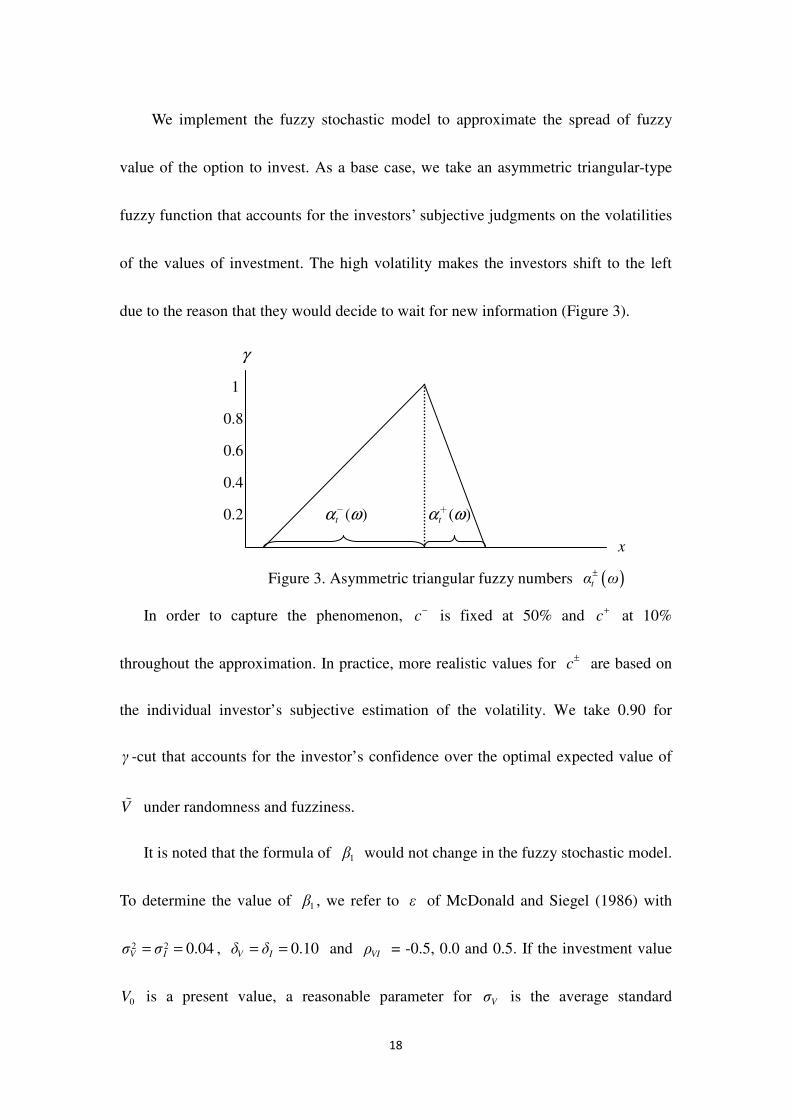
We implement the fuzzy stochastic model to approximate the spread of fuzzy

value of the option to invest. As a base case, we take an asymmetric triangular-type

fuzzy function that accounts for the investors’ subjective judgments on the volatilities

of the values of investment. The high volatility makes the investors shift to the left

due to the reason that they would decide to wait for new information (Figure 3).

γ

1

0.8

0.6

0.4

0.2 ( )tα ω−

( )tα ω+

x

Figure 3. Asymmetric triangular fuzzy numbers ( )tα ω±

In order to capture the phenomenon, c−

is fixed at 50% and c+

at 10%

throughout the approximation. In practice, more realistic values for c±

are based on

the individual investor’s subjective estimation of the volatility. We take 0.90 for

γ -cut that accounts for the investor’s confidence over the optimal expected value of

V under randomness and fuzziness.

It is noted that the formula of 1β would not change in the fuzzy stochastic model.

To determine the value of 1β , we refer to ε of McDonald and Siegel (1986) with

2 2 0.04V Iσ σ= = , 0.10V Iδ δ= = and VIρ = -0.5, 0.0 and 0.5. If the investment value

0V is a present value, a reasonable parameter for Vσ is the average standard

19

deviation for unlevered equity in the United States, which is about 0.20. Vδ

measures the extent to which the expected value increase in 0V alone fail to

compensate investors for the risk of value changes in 0V , which is set at 0.10.

Appropriate choices for 0I are less clear. If the investment cost is nonstochastic, Iδ

should be the risk-free rate. If 0I is systematically risky, but 0Iµ = , then it would

be greater.

Table 1. A comparison of the value of the option to invest under the fuzzy stochastic

model and the MS model ( 0 0 1V I= = )

Fuzzy stochastic model MS model

Vδ 0.10

VIρ -0.5 0.0 0.5 -0.5 0.0 0.5 2 2, V Iσ σ

0.01 [0.13, 0.15] [0.11, 0.13] [0.08, 0.09] 0.14 0.12 0.08

0.04 [0.24, 0.31] [0.20, 0.25] [0.15, 0.18] 0.27 0.23 0.16

0.30 [0.42, 0.84] [0.40, 0.68] [0.33, 0.49] 0.60 0.52 0.40

Iδ

0.01 [0.16, 0.20] [0.12, 0.14] [0.07, 0.08] 0.18 0.13 0.07

0.10 [0.24, 0.31] [0.20, 0.25] [0.15, 0.18] 0.27 0.23 0.16

0.25 [0.34, 0.51] [0.33, 0.47] [0.31, 0.43] 0.42 0.39 0.36

Note: Base case parameters are 2 2 0.04V Iσ σ= = and 0.10V Iδ δ= = . For fuzzy stochastic model,

entries are computed using (9), (20) and (22) in the current paper. For the MS model, entries are

computed using (4) and (12) in the text.

Table 1 compares the value of the option to invest under the fuzzy stochastic

model with the MS model. The entries in Table 1 represents the loss per dollar of V

if the investment were undertaken at 0 0 1V I = , rather than waiting until the optimal

time. The value of the option to invest can never exceed 0V , so 1.00 is an upper

bound for the entries in Table 1. For example, if 2 2 0.01V Iσ σ= = , 0VIρ = , and

0.10V Iδ δ= = , then the value of the option to invest is worth of 12 percent of 0V . To

20

conduct a comparative-static analysis, we let the other parameters stay the same but

the volatility increasing to 2 2 0.04V Iσ σ= = , then the value of the option would be 23

percent of 0V . Same to the above two examples, as the confidence level 0.90γ = ,

50%c−

= and 10%c+

= , the fuzzy value interval is [0.20, 0.25], noting that 0.23 is

included in the range. If the value of the option to invest is below the lower bound

0.20, then investing is likely to be postponed. If the value is above the upper bound

0.25, then investors will undertake the investment. If the value is below 0.25, the

pessimistic investors will decide to defer the investment due to the reason that they

need the larger value of the investment to overcome the investment failure. However,

if the value lies between 0.20 and 0.25, then the investment decisions of the investors

are vague. Because the optimistic investors are likely to decide to invest, the

pessimistic investors will not. For narrowing the closed interval, the investor can

increase the confidence level to decrease the width of the interval. Additionally, we

approximate a wide spread of parameters. It demonstrates that the value of the MS

model stay at any position of the closed interval.

Figure 4 conducts the sensitivity analysis of the fuzzy values of the option to

invest for these parameters, 1 2.16β = , 0.10V Iδ δ= = , 0.0

VIρ = , 0.5c

−= ,

0.1c+

= , 0.9γ = , and also for . 2 2 0.04V Iσ σ= = and 2 2 0.25

V Iσ σ= = . In each case,

the tangency point of ( )±

MS tF V with the line ( ) 1t t tC V I= = gives the values of the

21

fuzzy optimal investment threshold ( )( )( )* 1 1C ε ε γ c± ±= − ± − or

( )( )( )MS 1 1tV εI ε γ c∗± ±= − ± − . The value also shows that the simple NPV must be

modified to include the opportunity cost of investing now rather than waiting. The

opportunity cost is exactly ( )±

MS tF V . When MStV V ∗±< , ( ) MSMS t tF V V I± ∗±> − and

therefore ( )MS t MS tV I F V∗± ±< + : the value of the investment is less than its full cost, the

direct cost t

I plus the opportunity cost ( )±

MS tF V . (when MS tV I∗± = and ( )±

MS 0tF V =

for MS tV V∗± ≤ .) Note that ( )±

MS tF V increase when σ increases, as does the fuzzy

optimal investment threshold MSV ∗± . As a result, growth in t

V creates a value to

waiting, and increases the value of the option to invest.

0 0.2 0.4 0.6 0.8 1 1.2 1.4 1.6 1.80

0.1

0.2

0.3

0.4

0.5

0.6

0.7

0.8

0.9

Value of the Investmwent

Fu

zzy

Va

lue

of

the

Op

tion

to

In

ve

st

σ=0.25→

σ=0.04 →

V/I=1→

Figure 4. Fuzzy value of the option to invest, ( )±

MS tF V

Table 2 shows that the investment in the above first example would be optimal if

22

0 0V I reaches 1.37, and in the second example at 1.86. Table 2 clearly shows that the

level of 0 0V I at which the investment is optimal is typically much greater than 1.00.

Comparing with 0 0 1.37V I = , the fuzzy stochastic model shows that the lower and

upper bounds are 1.44 and 1.48. Comparing with 0 0 1.37V I = , they are 1,79 and

1.88.

Table 2. Value of benefit relative to investment cost ( 0 0V I ) at which investment is

optimal

Fuzzy stochastic model MS model

Vδ 0.10

VIρ -0.5 0.0 0.5 -0.5 0.0 0.5

2 2, V Iσ σ

0.01 [1.44, 1.48] [1.35, 1.38] [1.23, 1.25] 1.47 1.37 1.25

0.04 [2.02, 2.16] [1.79, 1.88] [1.52, 1.57] 2.13 1.86 1.56

0.30 [5.01, 6.70] [4.03, 4.98] [2.87, 3.26] 6.34 4.79 3.19

Iδ

0.01 [1.59, 1.65] [1.40, 1.44] [1.20, 1.22] 1.64 1.43 1.22

0.10 [2.02, 2.16] [1.79, 1.88] [1.52, 1.57] 2.13 1.86 1.56

0.25 [3.00, 3.44] [2.80, 3.16] [2.58, 2.86] 3.35 3.09 2.81

Note: Base case parameters are 2 2 0.04V Iσ σ= = and 0.10V Iδ δ= = . For fuzzy stochastic model,

entries are computed using (9), (20) and (22) in the current paper. For the MS model, entries are

computed using (4) and (12) in the text.

Further compare the value of the option to invest with the value under

uncertainty. Table 3 presents the percentage of the value of the option to invest which

is due to uncertainty. As the table shows, increase in Vδ , holding Iδ constant,

increases the uncertainty. As the table shows, increase in percentage of the value due

to uncertainty. When V Iδ δ≥ , all of the value is due to uncertainty, since otherwise

waiting would be suboptimal. The percentages presented by the MS model stay at the

closed intervals of the current proposed model.

Table 3. Percentage of value of the option to invest which is due to uncertainty

23

Fuzzy stochastic model MS model 2σ 0.04

0.02Vδ = [8.7, 9.6] 9.4

0.04Vδ = [19.8, 20.3] 20.1

0.06Vδ = [36.3, 36.5] 36.4

0.08Vδ = [61.8, 61.9] 61.9

0.10Vδ = 100.0 100.0

Note: All of these calculations assume that 0 0 1V I= = and 0.10Iδ = . For fuzzy stochastic model,

entries are computed using (9), (20) and (22) in the current paper. For the MS model, entries are

computed using (4), (12) and (13) in the text.

4.2 Fuzzy Goal

The fuzzy goal means a kind of utility for expected values of the option to invest,

and it represents the investor’s subjective judgment from the idea of Bellam and

Zadeh (1970). We follow Agliardi and Agliardi (2009) and show how the valuation

method works if fuzzy expectations are considered taking the investor’s subjective

utility function into account. Let ϕ denote a fuzzy goal, that is a continuous and

increasing function from [ )0, + ∞ to [ ]0, 1 , such that ( )0 0ϕ = and ( ) 1xϕ = as

x → ∞ . The fuzzy expectation under ϕ of a fuzzy number X is defined by ( ) ( ) ( ) sup ,

x R

E X X x x∈

= ϕ , (22)

and a rational expected value is defined as a real number where the fuzzy expectation

attains the supremum. The following argument is confined to determining the

expected fuzzy values of the option to invest.

Let the investor’s fuzzy goal, ϕ , be given. Define a grade *γ by

24

[ ] ( ) , MS 0: sup 0, 1 | , 0V V

γ γγ γ φ F V+ +−= ∈ ≤ , (23)

where ), γ γφ φ−= ∞ for ( )0, 1γ∈ and the supremum of the empty set is understood

to be 0. From equation (23) and the continuity of φ and , MSVγF

+ , we can easily check

( )0, MS, 0

V V

Vγ γφ F V

+

+ +− = . (24)

Proposition 5: Under the fuzzy expectation generated by possibility measures,

equation (22), the following (5a), and the following (5a) hold.

(5a) The membership degree of the fuzzy expectation of the values of the option to

invest MSVF is given by

( )( )MS 0 , 0V VE F Vγ

+

= . (25)

(5b) Further, the rational expected values of the option to invest is given by

V

V

γx φ

+

+

−= . (26)

Since the fuzzy expectation (22) is defined by possibility measures, equation (26)

gives an upper bound on rational expected values of the option to invest. Therefore,

similar to equation (26), another membership degree which gives a lower bound on

optimal expected values of the option to invest can be defined as follows:

V

V

γx φ

−

−

−= , (27)

where Vγ−

is defined by

[ ] ( ) , MS 0: sup 0, 1 | , 0VVγ γγ γ φ F V−− −= ∈ ≤ , (28)

25

and it satisfies

( )0, MS, 0V V

Vγ γφ F V

−

− −− = . (29)

Hence, from equations (23), (24), (25), (26), (27), (28) and (29), it can be easily

checked that the interval [ ], V Vx x− + is written as:

( ) ( ) ( ) *

* , MS 0, | , 0V

γx x x φ x F V x = ∈ ≤ R , (30)

which is the range of values x such that the membership degree of the expected

fuzzy values of the option to invest, ( )( ), MS 0 , 0V

γF V x , is greater than the degree of

the investor’s satisfaction, ( )φ x . Therefore, [ ], V Vx x− + means the investor’s

permissible range of expected values under his fuzzy goal φ .

Example: Let φ denote a fuzzy goal, that is continuous and increasing function

from [ )0, + ∞ , such that ( )0 0φ = and ( ) 1φ x → as x → +∞ .Assume that the

fuzzy goal, ( )i

cφ x ( 1, 2i = ), are defined as follows:

( )1 , 0,

0, 0.

iλ x

i e xφ x

x

− − ≥=

<. (31)

where iλ can be a view of the investor’s risk preference, or we say that the investors

have a constant absolute risk aversion (CARA) utility with the parameter iλ .

Equation (31) indicates that the fuzzy goal is ( ) 1 iλ xiφ x e−

= − if 0x ≥ and 0

otherwise. In nature, when the investors become more risk aversion, they tend to

increase the reference of the membership degree in the fuzzy set, thus causing the

narrow interval of the fuzzy values.

26

Going back to the base case we discuss in Section 4. The parameters of this

example is 0.10V Iδ δ= = , 0.0

VIρ = , 2 2 0.04

V Iσ σ= = , 2 0.08σ = , 2.16ε = ,

0.50c− = , 0.10c

+ = , 1 0.9λ = , and 2 0.4λ = . Higher value of λ represents more

degree of risk aversion.

0 0.05 0.1 0.15 0.2 0.25 0.3 0.35 0.40

0.1

0.2

0.3

0.4

0.5

0.6

0.7

0.8

0.9

1

Fuzzy Goal φ(x)

Me

mb

ers

hip

De

gre

e (

γ)

The Expected Fuzzy Values of the Option to Invest, F(x)

← γ*=0.62806

← γ*=0.56607

← γ*=0.87951

← γ*=0.86553

← φ (x)=1-e-0.9x

← φ (x)=1-e-0.4x

Figure 5. Membership degree ( γ ), expected fuzzy values of the option to invest

optimal fuzzy value ( )±

MS tF V , and fuzzy goal ( )φ x

From Figure 5, we find that the membership level of the fuzzy expectation of

fuzzy values are *

*, γ γ = [ ]0.8655, 0.8795 , and *

*, γ γ = [ ]0.5661, 0.6281 for

fuzzy goal equals to equation (27) with 1 0.9λ = and 2 0.4λ = , respectively, this

membership level means that the degrees of the investor’s satisfaction in valuing. The

27

corresponding permissible range for the fuzzy values of the option to invest under the

fuzzy goals are *

*, x x = [ ]0.2229, 0.2351 , and *

*, x x = [ ]0.2087, 0.2473 ,

respectively. It is clear that the interval difference in the higher risk aversion ( 1 0.9λ = )

is 0.0122, which is smaller than 0.0386 in the lower risk aversion ( 2 0.4λ = ). This

evidence indicates that an increase in λ in the CARA utility will narrow the range of

the expected fuzzy values. Another useful interpretation is that the narrow range will

easily cause the investors with high risk aversion to defer their investment, that is,

they believe that waiting is better than investing, as we discuss in the Introduction and

Equation (12). As fuzzy factor c− and c

− approach zero, the fuzzy values would

converge to the MS model.

5. Concluding Remarks

This paper introduces fuzziness to the stochastic process for evaluating the

option to invest in an irreversible investment. The existing stochastic process simply

deals with the randomness as uncertainty over the volatility of the value of the

investment, in which the value of the investment is assumed to follow the geometric

Brownian motion. In effect, the investors’ heterogeneities on the volatility are likely

to be quite different, but they cannot be modeled by the existing stochastic process.

Our first addition of the investors’ subjective judgments modeled by the fuzziness to

28

the stochastic model is one of our major contributions. Thus, our model can consider

the fuzziness as uncertainty to define the fuzzy values of the investment. The

fuzziness is subject to the changes of the membership degrees such that the investors

can increase the membership degree to decrease the interval of the fuzzy values. This

fact points to the influences of the optimism and pessimism in making the investment

decisions.

We also contribute showing how to incorporate triangular fuzzy numbers into the

existing stochastic process. The incorporation is a subjective new development in

evaluating the option to invest. The development can help explain the properties of

the investment decisions of the optimistic and pessimistic investors. We also hope that

the methods for the numerical computation of the optimal grade of the investor’s

confidence, and the corresponding optimal interval of the fuzzy values will be

employed in practice. If necessary, the further research may develop a defuzzified

method to find a crisp value from the interval of the fuzzy values.

29

Appendix:

1. Proof of Proposition 2

We expand dF of the Bellman equation ( )tρFdt E dF= using Ito’s Lemma,

and we use primes to denote derivatives, for example, V

F dF dV= and

2 2

VVF d F dV= . Then

( )21

2V VVdF F dV F dV= + . (A1)

The above expression is substituted with equation (1) for dV , and ( )E dz is

zero. This gives

( ) 2 21

2V V V VVE dF µ VF dt σ V F dt= + . (A2)

After dividing through dt , the Bellman equation becomes:

( )2 2

S

10

2V t VV V t V tσ V F µ V F ρF V+ − = . (A3)

Additionally, the value of the option to invest ( )S tF V must satisfy the following

boundary conditions:2

( )S 0 0F = , (A4)

( )* *SF V V I= − , (A5)

( )*, S 1VF V = . (A6)

Since the second-order homogeneous differential equation (A3) is linear in the

dependent variable F and its derivatives, its general solution can be expressed as a

2 Condition (A4) is the initial condition which indicates that if tV is zero, then the value of the option

to invest will be zero. Condition (A5) is the value-matching condition which indicates that if the firm

invests, then the firm receives a net payoff *V I− . Condition (A6) is the smooth-pasting condition

which indicates that if ( )S tF V were not continuous and smooth at the investment threshold *V , then

one could do better by exercising as a different point.

30

linear combination of any two independent solutions. If we try the function β

tAV , we

see by substitution that it satisfies the equation provides β is a root of the quadratic

equation. When ( )Sβ

t tF V AV= , we can obtain 1β

V tF βAV

−= and

( ) 21 β

VV tF β β AV−= − . Substituting them into equation (A3) gives

( )211 0

2 V Vσ β β µ β r− + − = . (A7)

The two roots are

( )2

1 2 2 2

1 12 1

2 2V V

V V V

µ µ ρβ

σ σ σ

= − + − + >

, (A8)

and

( )2

2 2 2 2

1 12 0

2 2V V

V V V

µ µ rβ

σ σ σ

= − − − + <

. (A9)

The value of β cannot be less than 1 to yield the positive optimal investment

threshold. Note that equation (A3) is a second-order differential equation, but there

are three boundary conditions that must be satisfied. The reason is that although the

position of the first boundary ( 0V = ) is known, the position of the second boundary

is not, in other words, the “free boundary” *V must be determined as part of the

solution. That needs the third condition.

To satisfy the boundary condition (A4), the solution for the value of the option to

invest must take the form

31

( ) 1

Sβ

t tF V AV=3, (A10)

where A is a constant that will be determined, and 1 1β > is a known constant

whose value depends on the parameters µ , σ , and ρ of the differential equation.

The remaining boundary conditions, (A5) and (A6), can be used to solve the two

remaining unknowns constant A , and the optimal investment threshold *V at

which it is optimal to invest. By substituting (A10) into (A5) and (A6) and

rearranging, we obtain that

* 1

1 1

βV I

β=

−, (A11)

and

( )

( )( )

1

1

11

*1

1 1 1

1 1

1

βββ

A I Vβ β β

− −− −

= = −

. (A12)

By plugging equation (A11) and (A12) into the ( ) 1

Sβ

t tF V AV= and rearranging,

we find the value of the option to invest:

1

* *

S **

1

, if ,

( ) 1, if .

1

t

β

t tt

V I V V

F V VI V V

β V

− ≥

= < −

(A13)

2. Proof of Proposition 3

Equation (9) shows ( ), ( ) 1 (1 ) ( )t γ tV ω γ c V ω± ±= ± − . The Ito’s Lemma is used as

the usual rules of calculus to define this differential in terms of first-order changes in

3 The general solution should be ( ) 1 2S 1 2

β βt t tF V AV A V= + . When 2 0β < and 0V = , the value of

the option to invest will become ∞ . This violates the boundary condition (A4), ( )S 0 0F = . So, 2A

must be zero leaving the solution ( ) 1Sβ

t tF V AV= .

32

V± :

( )t t V V VdV V µ dt σ dz± ±= + . (A14)

Now we are ready to examine the investor’s optimal investment rule. For

algebraic simplicity we will again assume an exogenously specified discount rate, and

use the dynamic programming approach. Let the fuzzy stochastic process of the

Bellman equation be ( )tρF dt E dF± ±= . By expanding dF± with Ito’s Lemma, we

obtain ( )221

2t V VV

E dF µV F dt σ V F dt± ± ± ± ±= + . So, the Bellman equation can be

rewritten as 2 210

2V VVV Vσ V F µ VFF rF

± ± ±+ − = . In addition, the fuzzy values of the

option to invest ( )S tF V± must satisfy the following boundary conditions: the initial

condition ( )S 0 0F± = , the value-matching condition ( )* *

SF V V I± ± ±= − , and the

smooth-pasting condition ( ) ( )( )*, S 1 1VF V γ c± ± ±= ± − . This condition means that if

VF ± are not continuous and smooth at the fuzzy optimal investment thresholds *V

± ,

the investors could invest better at a different point (Dixit, 1988).

By adopting the similar way to (A10), we find two unknowns constant A±

and the optimal investment threshold *V ± :

( )( )

* 1

1 1 1

βV I

β γ c

±

±=

− ± − , (A15)

and

( )( )

( )1( 1)

*

1

1 1 βγ cA V

β

±− −

± ±± −

= . (A16)

33

We then plug equation (A15) and (A16) into the ( ) ( ) 1

S

β

t tF V A V± ±= . Thus,

( ) ( )( )( )( )

1

* *

S *

*

1

, if ,

1 1, if .

1 1

t

βt t

t

V I V V

γ cF V VI V V

Vβ γ c

± ±

±±

±

±±

− ≥ ± −= < − ± −

(A17)

3. Proof of Proposition 4

Under equation (14), we first write down the heterogeneous fuzzy values of the

option to invest:

( ) ( )MS 1

ε

tt t

CF C C I

C

± ∗±

∗±

= −

, (A18)

and using the similar method for equation (A15) to find the optimal investment

threshold *C

± :

( )( )

* 1

1 1 1

βC

β γ c

±

±=

− ± −. (A19)

Because of the adjustment discount rate in market equilibrium, now equation

(A19) can be rewritten by applying 1β ε= to obtain the formula

( )( )*

1 1

εC

ε γ c

±

±=

− ± −, and simply plugging this formula to find the solution for the

fuzzy values of the option to invest at time t in equation (A17):

( )

( )

( )( )( )( )

1

* *

±

MS*

*

1 , if ,

1 1, if .

1 1

t t

βt

tt t

C I C C

F C γ c CI C C

Cε γ c

± ±

±

±

±±

− ≥ = ± − < − ± −

. (A20)

34

References Adda, J. and R. Cooper, “Dynamic Economics: Quantitative Methods and

Applications.” The MIT press, Cambridge, Massachusetts, London, England,

(2003).

Basak, S., “A Model of Dynamic Equilibrium Asset Pricing with Heterogeneous

Beliefs and Extraneous Risk.” Journal of Economic Dynamics & Control 24(1),

63-95, (2000).

Bellman, R. E. and L. A. Zadeh, “Decision-Making in a Fuzzy Environment.”

Management Science 17(4), 141-164, (1970).

Benninga, S. and J. Mayshar, “Heterogeneity and Option Pricing.” Working paper,

Wharton School, (1997).

Brennan, M., “The Pricing of Contingent Claims in Discrete Time Models.” Journal

of Finance 34(1), 53-68, (1979).

Caballero, R. J., “On the Sign of the Investment–Uncertainty Relationship.” American

Economic Review 81(1), 279-288, (1991).

Daniel, K. D., D. Hirshfeiler and A. Subrahmanyam, “Overconfidence, Arbitrage and

Equilibrium Assets Pricing.” Journal of Finance 6(3), 921-965, (2001).

De Bondt, W. P. M., “Betting on Trends: Intuitive Forecasts of Financial Risk and

Return.” International Journal of Forecasting 9(3), 355-371, (1993).

Detemple, J. and S. Murthy, “Intertemporal Asset Pricing with Heterogeneous

Beliefs.” Journal of Economic Theory 62(2), 294-320, (1994).

Dixit, A., "A Heuristic Argument for the Smooth Pasting Condition." Unpub.,

Princeton U., Mar, (1988).

Dixit, A. K. and R. S. Pindyck, “ Investment under Uncertainty.” Princeton University

Press, (1994).

Harris, M. and A. Raviv, “Differences of Opinion make a Horserace.” Review of

Financial Studies 6(3), 473-506, (1993).

Leahy, J. V. and T. M. Whited, “The Effect of Uncertainty on Investment: Some

Stylized Facts.” Journal of Money, Credit, and Banking 28(1), 64-83, (1996).

35

Malliaris, A. G. and W. A. Brock, “Stochastic Methods in Economics and Finance.”

NY: North-Hol- land, (1982).

Mankiw, G. N. and S. P. Zeldes, “The Consumption of Stockholders and

Nonstockholders.” Journal of Financial Economics 29(1), 97-112, (1991).

McDonald, R. and D. Siegel, “The Value of Waiting to Invest.” Quarterly Journal of

Economics 101(4), 707-728, (1986).

Pindyck, R. S., “Irreversibility, Uncertainty, and Investment.”Journal of Economic

Literature 29(3), 1110-1152, (1991).

Peskir, G. and A. Shiryaev, “Optimal Stopping and Free-Boundary Problems.”

Birhauser Verlag, Basel, Boston, Berlin, (2006).

Peters, E. “Chaos and Order in the Capital Markets”, 2ª edição. New York: Wiley,

(1996).

Peters, E., “Simple and Complex Market Inefficiencies: Integrating Efficient Markets,

Behavioral Finance, and Complexity.” Journal of Behavioral Finance 4(4),

225-233, (2003).

Robinstein, M., “The Fundamental Theorem of Parameter-Preference Security

Valuation.” Journal of Financial and Quantitative Analysis 8(1), 61-69, (1973).

Robinstein, M., “Implied Binominal Trees.” Journal of Finance 49(3), 771-818,

(1994).

Ross, S. M., “An Introduction to Mathematical Finance.” Cambridge University Press,

Cambridge, (1999).

Sarkar, S., “On the Investment-Uncertainty Relationship in a Real Options Model.”

Journal of Economic Dynamics & Control 24(2), 219-225, (2000).

Sarkar, S., “The Effect of Mean Reversion on Investment under Uncertainty.” Journal

of Economic Dynamics & Control 28(2), 377-396, (2003).

Shefrin, H. and M. Statman, “Behavioral Capital Asset Pricing Theory.” Journal of

Financial and Quantitative Analysis 29(3), 323-349, (1994)

Stapleton, R. C. and M. G. Subrahmanyam, “The Valuation of Options When Asset

Returns are Generated by Binominal Process.” Journal of Finance 39(5),

36

1525-1539, (1984).

Yoshida, Y., “A Discrete-Time Model of American Put Option in An Uncertain

Environment.” European Journal of Operational Research 151(1), 153-166,

(2003).