Real Numbers and Computational Complexity

Real Numbers and Computational Complexity

Norbert Müller

[email protected]

FB IV – InformatikUniversität Trier

Norbert Müller (Trier) Darmstadt, 2012-10-05 1 / 34

mailto:[email protected]

Introduction

1 Introduction

2 Computational complexity / efficient algorithms

3 Real vs. discrete computational complexity


Introduction

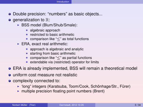
Double precision: “numbers” as basic objects...generalization to R:

I BSS model (Blum/Shub/Smale):F algebraic approachF restricted to basic arithmeticF comparison like “≤” as total functions

I ERA, exact real arithmetic:F approach is algebraic and analyticF starting from basic arithmeticF comparison like “≤” as partial functionsF extendable via (restricted) operator for limits

ERA is already implemented, BSS will remain a theoretical modeluniform cost measure not realisticcomplexity connected to:

I ‘long” integers (Karatsuba, Toom/Cook, Schönhage/Str., Fürer)I multiple precision floating point numbers (Brent)


Introduction

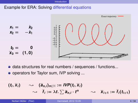
Example for ERA: Solving differential equations

x1 = x2x2 = −x1

t0 = 0x0 = (1, 0)

Exact trajectory

0 5 10 15 20 25−1−0.8−0.6−0.4−0.2 0 0.2 0.4 0.6 0.8 1

−1−0.8−0.6−0.4−0.2

0 0.2 0.4 0.6 0.8

1

data structures for real numbers / sequences / functions...operators for Taylor sum, IVP solving ...

(ti , x i) ; (an,i)n∈N := IVP(ti , x i)

; f i := λt.∑

an,i · tn ; x i+1 := f i(ti+1)


Introduction

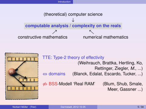
(theoretical) computer science↓

computable analysis / complexity on the reals↗ ↖

constructive mathematics numerical mathematics

TTE: Type-2 theory of effectivity(Weihrauch, Brattka, Hertling, Ko,

Rettinger, Ziegler, M., ...)⇔ domains (Blanck, Edalat, Escardo, Tucker, ...)

6⇔ BSS-Modell ‘Real RAM’ (Blum, Shub, Smale,Meer, Gassner ...)


Introduction

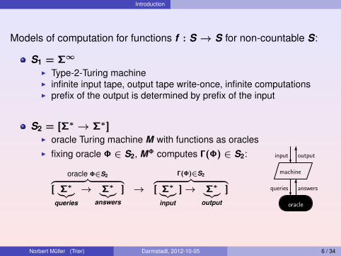
Models of computation for functions f : S → S for non-countable S:

S1 = Σ∞

I Type-2-Turing machineI infinite input tape, output tape write-once, infinite computationsI prefix of the output is determined by prefix of the input

S2 = [Σ∗ → Σ∗]I oracle Turing machine M with functions as oracles

machine

queries answers

input output

oracle

I fixing oracle Φ ∈ S2, MΦ computes Γ(Φ) ∈ S2:

oracle Φ∈S2︷︸︸︷[ Σ∗︸︷︷︸queries

→ Σ∗︸︷︷︸answers

] →

Γ(Φ)∈S2︷︸︸︷[ Σ∗︸︷︷︸

input

]→ Σ∗︸︷︷︸output

]


Introduction

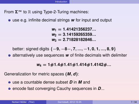
From Σ∞ to R using Type-2-Turing machines:

use e.g. infinite decimal strings w for input and output

w1 = 1.41421356237...w2 = 3.14159265359...w3 = 2.71828182846...

better: signed digits {−9,−8−, 7, ...,−1, 0, 1, ..., 8, 9}alternatively use sequences w of finite decimals with delimiter

w4 = 1#1.4#1.41#1.414#1.4142#...

Generalization for metric spaces (M, d):

use a countable dense subset D in M andencode fast converging Cauchy sequences in D...


Introduction

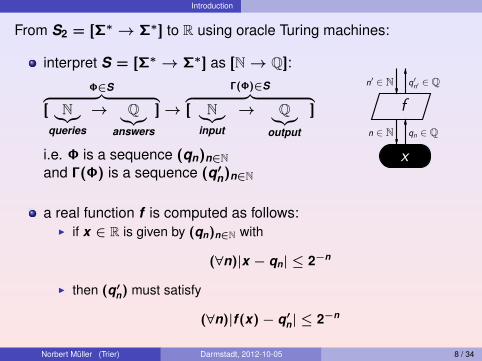
From S2 = [Σ∗ → Σ∗] to R using oracle Turing machines:

interpret S = [Σ∗ → Σ∗] as [N→ Q]:

Φ∈S︷︸︸︷[ N︸︷︷︸queries

→ Q︸︷︷︸answers

]→Γ(Φ)∈S︷︸︸︷

[ N︸︷︷︸input

→ Q︸︷︷︸output

]

i.e. Φ is a sequence (qn)n∈Nand Γ(Φ) is a sequence (q′n)n∈N

n′ ∈ N

n ∈ N

q′n′ ∈ Q

qn ∈ Q

f

x

a real function f is computed as follows:I if x ∈ R is given by (qn)n∈N with

(∀n)|x − qn| ≤ 2−n

I then (q′n) must satisfy

(∀n)|f (x)− q′n| ≤ 2−n


Introduction

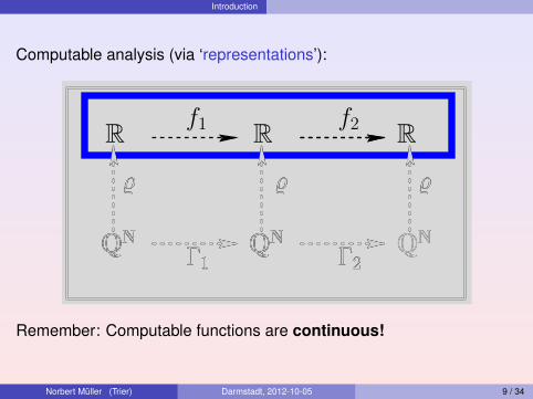
Computable analysis (via ‘representations’):

R f1 f2R R

QN

%% %

Γ1 Γ2QN QN

%% %

Γ1 Γ2QN QN

%% %

Γ1 Γ2QN QN QN

Remember: Computable functions are continuous!


Computational complexity / efficient algorithms

1 Introduction





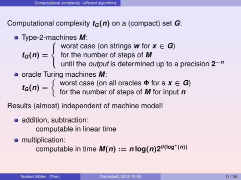
Computational complexity tG(n) on a (compact) set G:

Type-2-machines M :

tG(n) =

worst case (on strings w for x ∈ G)for the number of steps of Muntil the output is determined up to a precision 2−n

oracle Turing machines M :

tG(n) =

{worst case (on all oracles Φ for a x ∈ G)for the number of steps of M for input n

Results (almost) independent of machine model!

addition, subtraction:computable in linear time

multiplication:computable in time M(n) := n log(n)2θ(log∗(n))



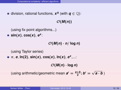
division, rational functions, xq (with q ∈ Q):

O(M(n))

(using fix point algorithms...)sin(x), cos(x), ex :

O(M(n) · n/ log n)

(using Taylor series)π, e, ln(2), sin(x), cos(x), ln(x), ex ,...:

O(M(n) · log n)

(using arithmetic/geometric mean a′ = a+b2 ; b′ =

√a · b )



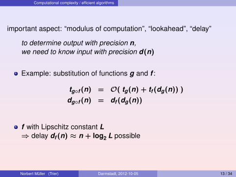
important aspect: “modulus of computation”, “lookahead”, “delay”

to determine output with precision n,we need to know input with precision d(n)

Example: substitution of functions g and f :

tg◦f (n) = O( tg(n) + tf (dg(n)) )

dg◦f (n) = df (dg(n))

f with Lipschitz constant L⇒ delay df (n) ≈ n + log2 L possible



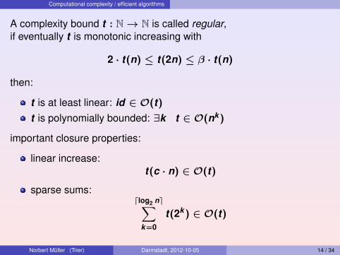
A complexity bound t : N→ N is called regular,if eventually t is monotonic increasing with

2 · t(n) ≤ t(2n) ≤ β · t(n)

then:

t is at least linear: id ∈ O(t)

t is polynomially bounded: ∃k t ∈ O(nk )

important closure properties:

linear increase:t(c · n) ∈ O(t)

sparse sums:dlog2 ne∑

k=0

t(2k ) ∈ O(t)



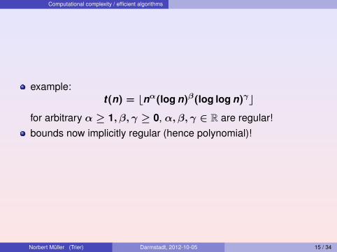
example:t(n) = bnα(log n)β(log log n)γc

for arbitrary α ≥ 1, β, γ ≥ 0, α, β, γ ∈ R are regular!bounds now implicitly regular (hence polynomial)!



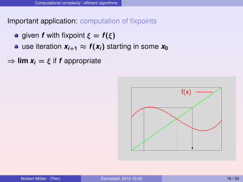
Important application: computation of fixpoints

given f with fixpoint ξ = f (ξ)

use iteration xi+1 ≈ f (xi) starting in some x0

⇒ lim xi = ξ if f appropriate

f(x)



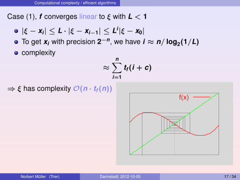
Case (1), f converges linear to ξ with L < 1

|ξ − xi | ≤ L · |ξ − xi−1| ≤ Li |ξ − x0|To get xi with precision 2−n, we have i ≈ n/ log2(1/L)

complexity

≈n∑

i=1

tf (i + c)

⇒ ξ has complexity O(n · tf (n))f(x)



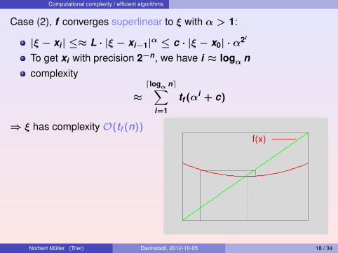
Case (2), f converges superlinear to ξ with α > 1:

|ξ − xi | ≤≈ L · |ξ − xi−1|α ≤ c · |ξ − x0| · α2i

To get xi with precision 2−n, we have i ≈ logα ncomplexity

≈dlogα ne∑

i=1

tf (αi + c)

⇒ ξ has complexity O(tf (n))f(x)



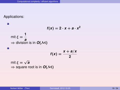
Applications:

f (x) = 2 · x + a · x2

mit ξ =1a

⇒ division is in O(M)

f (x) =x + a/x

2

mit ξ =√

a⇒ square root is in O(M)



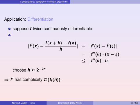
Application: Differentiation

suppose f twice continuously differentiable

|f ′(x)−f (x + h)− f (x)

h| = |f ′(x)− f ′(ξ)|

= |f ′′(θ) · (x − ξ)|≤ |f ′′(θ) · h|

choose h ≈ 2−2n

⇒ f ′ has complexity O(tf (n)).



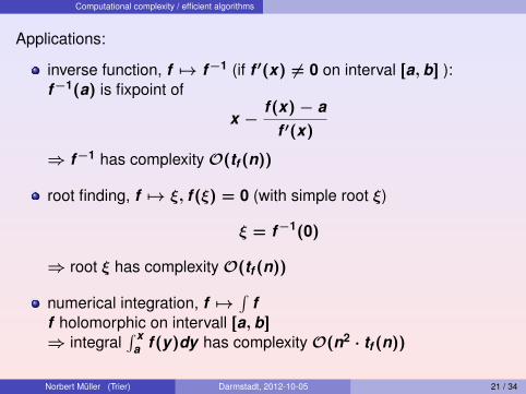
Applications:

inverse function, f 7→ f−1 (if f ′(x) 6= 0 on interval [a, b] ):f−1(a) is fixpoint of

x −f (x)− a

f ′(x)

⇒ f−1 has complexity O(tf (n))

root finding, f 7→ ξ, f (ξ) = 0 (with simple root ξ)

ξ = f−1(0)

⇒ root ξ has complexity O(tf (n))

numerical integration, f 7→∫

ff holomorphic on intervall [a, b]⇒ integral

∫ xa f (y)dy has complexity O(n2 · tf (n))


Real vs. discrete computational complexity

1 Introduction





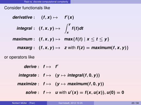
Consider functionals like

derivative : (f , x) 7→ f ′(x)

integral : (f , x, y) 7→∫ y

xf (t)dt

maximum : (f , x, y) 7→ max{f (t) | x ≤ t ≤ y}

maxarg : (f , x, y) 7→ z with f (z) = maximum(f , x, y)}

or operators like

derive : f 7→ f ′

integrate : f 7→ (y 7→ integral(f , 0, y))

maximize : f 7→ (y 7→ maximum(f , 0, y))

solve : f 7→ u with u′(x) = f (x, u(x)), u(0) = 0



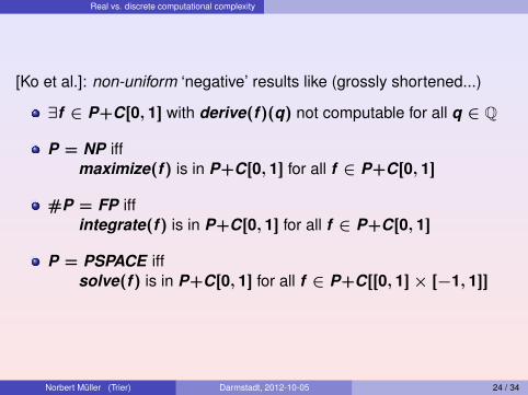
[Ko et al.]: non-uniform ‘negative’ results like (grossly shortened...)

∃f ∈ P+C[0, 1] with derive(f )(q) not computable for all q ∈ Q

P = NP iffmaximize(f ) is in P+C[0, 1] for all f ∈ P+C[0, 1]

#P = FP iffintegrate(f ) is in P+C[0, 1] for all f ∈ P+C[0, 1]

P = PSPACE iffsolve(f ) is in P+C[0, 1] for all f ∈ P+C[[0, 1]× [−1, 1]]



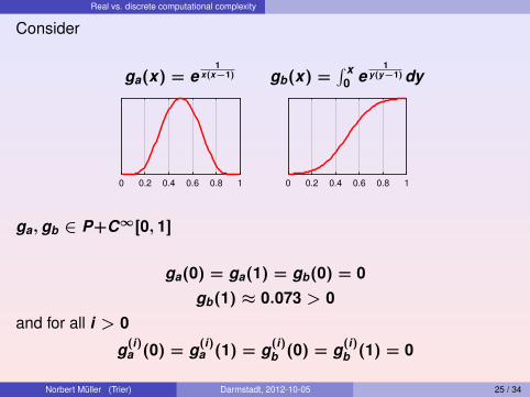
Consider

ga(x) = e1

x(x−1) gb(x) =∫ x

0 e1

y(y−1) dy

0 0.2 0.4 0.6 0.8 1 0 0.2 0.4 0.6 0.8 1

ga, gb ∈ P+C∞[0, 1]

ga(0) = ga(1) = gb(0) = 0gb(1) ≈ 0.073 > 0

and for all i > 0

g(i)a (0) = g(i)

a (1) = g(i)b (0) = g(i)

b (1) = 0



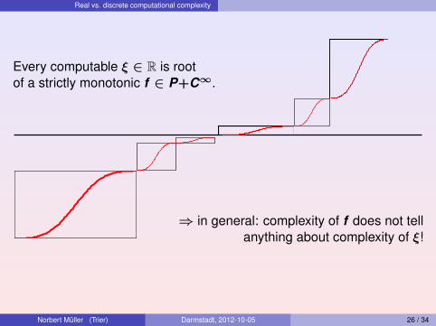
Every computable ξ ∈ R is rootof a strictly monotonic f ∈ P+C∞.

⇒ in general: complexity of f does not tellanything about complexity of ξ!



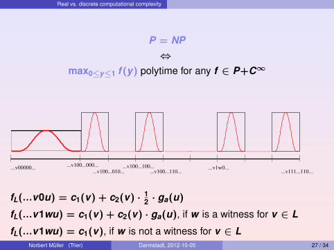
P = NP⇔

max0≤y≤1 f (y) polytime for any f ∈ P+C∞

...v100...010...

...v100...000... ...v100...100...

...v100...110......v1w0......v00000...

...v111...110...

fL(...v0u) = c1(v) + c2(v) · 12 · ga(u)

fL(...v1wu) = c1(v) + c2(v) · ga(u), if w is a witness for v ∈ L

fL(...v1wu) = c1(v), if w is not a witness for v ∈ LNorbert Müller (Trier) Darmstadt, 2012-10-05 27 / 34


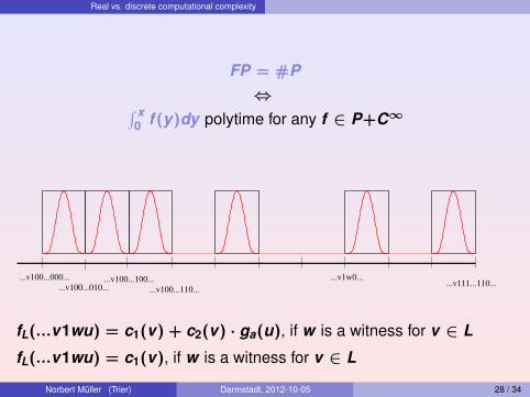
FP = #P⇔∫ x

0 f (y)dy polytime for any f ∈ P+C∞

...v1w0......v111...110...

...v100...000...

...v100...010...

...v100...100...

...v100...110...

fL(...v1wu) = c1(v) + c2(v) · ga(u), if w is a witness for v ∈ L

fL(...v1wu) = c1(v), if w is a witness for v ∈ L



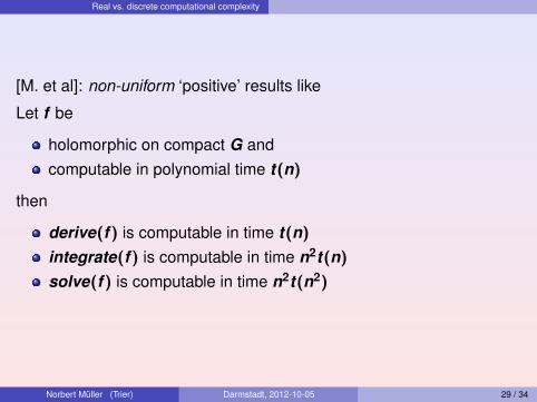
[M. et al]: non-uniform ‘positive’ results like

Let f be

holomorphic on compact G andcomputable in polynomial time t(n)

then

derive(f ) is computable in time t(n)

integrate(f ) is computable in time n2t(n)

solve(f ) is computable in time n2t(n2)



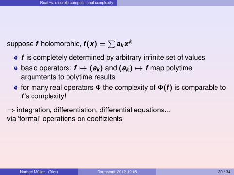
suppose f holomorphic, f (x) =∑

ak xk

f is completely determined by arbitrary infinite set of valuesbasic operators: f 7→ (ak ) and (ak ) 7→ f map polytimeargumtents to polytime resultsfor many real operators Φ the complexity of Φ(f ) is comparable tof ’s complexity!

⇒ integration, differentiation, differential equations...via ‘formal’ operations on coeffizients



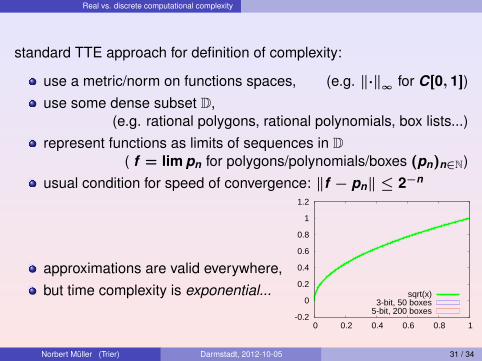
standard TTE approach for definition of complexity:

use a metric/norm on functions spaces, (e.g. ‖·‖∞ for C[0, 1])use some dense subset D,

(e.g. rational polygons, rational polynomials, box lists...)represent functions as limits of sequences in D

( f = lim pn for polygons/polynomials/boxes (pn)n∈N)usual condition for speed of convergence: ‖f − pn‖ ≤ 2−n

-0.2

0

0.2

0.4

0.6

0.8

1

1.2

0 0.2 0.4 0.6 0.8 1

sqrt(x)3-bit, 50 boxes

5-bit, 200 boxes

approximations are valid everywhere,but time complexity is exponential...



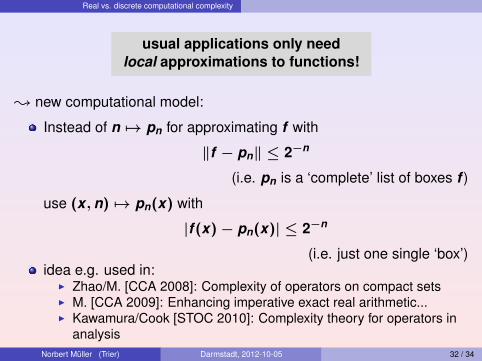
usual applications only needlocal approximations to functions!

; new computational model:

Instead of n 7→ pn for approximating f with

‖f − pn‖ ≤ 2−n

(i.e. pn is a ‘complete’ list of boxes f )

use (x, n) 7→ pn(x) with

|f (x)− pn(x)| ≤ 2−n

(i.e. just one single ‘box’)idea e.g. used in:

I Zhao/M. [CCA 2008]: Complexity of operators on compact setsI M. [CCA 2009]: Enhancing imperative exact real arithmetic...I Kawamura/Cook [STOC 2010]: Complexity theory for operators in

analysisNorbert Müller (Trier) Darmstadt, 2012-10-05 32 / 34


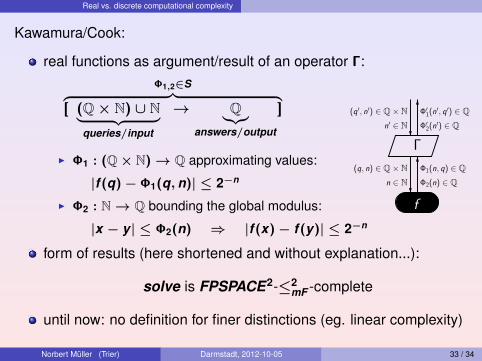
Kawamura/Cook:

real functions as argument/result of an operator Γ:Φ1,2∈S︷︸︸︷

[ (Q× N) ∪ N︸︷︷︸queries/input

→ Q︸︷︷︸answers/output

]n′ ∈ N

(q, n) ∈ Q×N

Γ

n ∈ N

(q′, n′) ∈ Q×N

Φ1(n, q) ∈ QΦ2(n) ∈ Q

Φ′2(n′) ∈ QΦ′1(n′, q′) ∈ Q

f

I Φ1 : (Q× N)→ Q approximating values:

|f (q)− Φ1(q, n)| ≤ 2−n

I Φ2 : N→ Q bounding the global modulus:

|x − y | ≤ Φ2(n) ⇒ |f (x)− f (y)| ≤ 2−n

form of results (here shortened and without explanation...):

solve is FPSPACE2-≤2mF -complete

until now: no definition for finer distinctions (eg. linear complexity)



Thank you for your attention!

Any questions or remarks?


Documents

Real Numbers and Computational Complexity