Embed Size (px)
Citation preview
Introduction to Computational ComplexityA 10-lectures Graduate Course
Martin Stigge, [email protected]
Uppsala University, Sweden
13.7. - 17.7.2009
Martin Stigge (Uppsala University, SE) Computational Complexity Course 13.7. - 17.7.2009 1 / 148
Introduction
Administrative Meta-Information
5-Day course, Monday (13.7.) to Friday (17.7.)
Schedule:
Mon (13.7.): 10:00 - 12:00, 16:30 - 18:30Tue (14.7.): 10:00 - 12:00, 14:00 - 16:00
Wed (15.7.): 10:00 - 12:00, 14:00 - 16:00Thu (16.7.): 10:00 - 12:00, 14:00 - 16:00
Fri (17.7.): 10:00 - 12:00, 16:30 - 18:30
Lecture notes avaiable at:
http://www.it.uu.se/katalog/marst984/cc-st09
Some small assignments at end of day
Course credits: ??
Course is interactive, so:
Any questions so far?
Martin Stigge (Uppsala University, SE) Computational Complexity Course 13.7. - 17.7.2009 2 / 148
Introduction
What is Computational Complexity?
Studies intrinsic complexity of computational tasks
Absolute Questions:I How much time is needed to perform the task?I How much resources will be needed?
Relative Questions:I More difficult than other tasks?I Are there “most difficult” tasks?
(Surprisingly: Many relative answers, only few absolute ones..)
Rigorous treatment:I Mathematical formalisms, minimize “hand-waving”I Precise definitionsI Theorems have to be proved
After all: Complexity Theory
Martin Stigge (Uppsala University, SE) Computational Complexity Course 13.7. - 17.7.2009 3 / 148
Introduction
What is Computational Complexity? (Cont.)
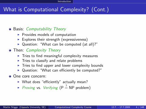
Basis: Computability TheoryI Provides models of computationI Explores their strength (expressiveness)I Question: “What can be computed (at all)?”
Then: Complexity TheoryI Tries to find meaningful complexity measuresI Tries to classify and relate problemsI Tries to find upper and lower complexity boundsI Question: “What can efficiently be computed?”
One core concern:I What does “efficiently” actually mean?
I Proving vs. Verifying (P?= NP problem)
Martin Stigge (Uppsala University, SE) Computational Complexity Course 13.7. - 17.7.2009 4 / 148
Introduction
Course Outline
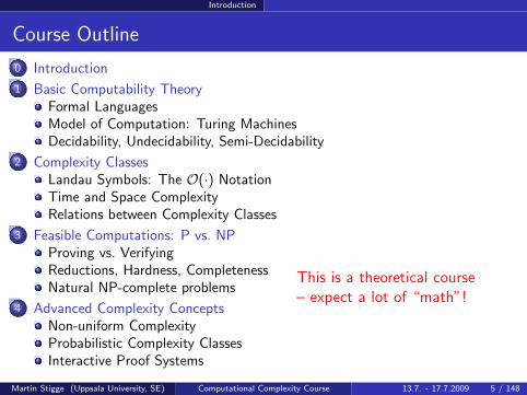
0 Introduction
1 Basic Computability TheoryFormal LanguagesModel of Computation: Turing MachinesDecidability, Undecidability, Semi-Decidability
2 Complexity ClassesLandau Symbols: The O(·) NotationTime and Space ComplexityRelations between Complexity Classes
3 Feasible Computations: P vs. NPProving vs. VerifyingReductions, Hardness, CompletenessNatural NP-complete problems
4 Advanced Complexity ConceptsNon-uniform ComplexityProbabilistic Complexity ClassesInteractive Proof Systems
Martin Stigge (Uppsala University, SE) Computational Complexity Course 13.7. - 17.7.2009 5 / 148
This is a theoretical course– expect a lot of “math”!
Basic Computability Theory Formal Languages
Problems as Formal Languages
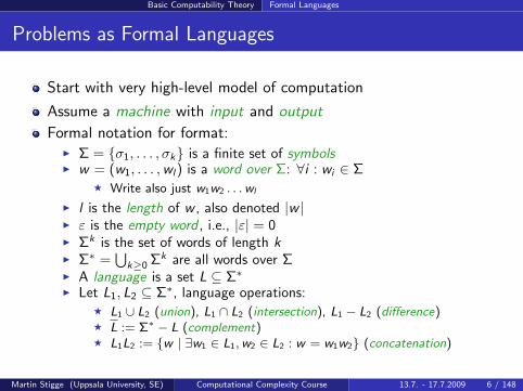
Start with very high-level model of computation
Assume a machine with input and output
Formal notation for format:I Σ = σ1, . . . , σk is a finite set of symbolsI w = (w1, . . . ,wl) is a word over Σ: ∀i : wi ∈ Σ
F Write also just w1w2 . . . wl
I l is the length of w , also denoted |w |I ε is the empty word , i.e., |ε| = 0I Σk is the set of words of length kI Σ∗ =
⋃k≥0 Σk are all words over Σ
I A language is a set L ⊆ Σ∗
I Let L1, L2 ⊆ Σ∗, language operations:F L1 ∪ L2 (union), L1 ∩ L2 (intersection), L1 − L2 (difference)F L := Σ∗ − L (complement)F L1L2 := w | ∃w1 ∈ L1, w2 ∈ L2 : w = w1w2 (concatenation)
Martin Stigge (Uppsala University, SE) Computational Complexity Course 13.7. - 17.7.2009 6 / 148
Basic Computability Theory Formal Languages
Problems as Formal Languages (Example)
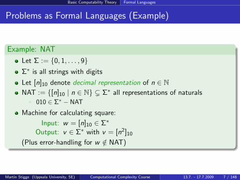
Example: NAT
Let Σ := 0, 1, . . . , 9Σ∗ is all strings with digits
Let [n]10 denote decimal representation of n ∈ NNAT := [n]10 | n ∈ N ( Σ∗ all representations of naturals
I 010 ∈ Σ∗ − NAT
Machine for calculating square:
Input: w = [n]10 ∈ Σ∗
Output: v ∈ Σ∗ with v = [n2]10
(Plus error-handling for w /∈ NAT)
Martin Stigge (Uppsala University, SE) Computational Complexity Course 13.7. - 17.7.2009 7 / 148
Basic Computability Theory Formal Languages
Problems as Formal Languages (2nd Example)
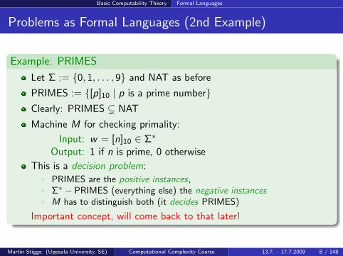
Example: PRIMES
Let Σ := 0, 1, . . . , 9 and NAT as before
PRIMES := [p]10 | p is a prime numberClearly: PRIMES ( NAT
Machine M for checking primality:
Input: w = [n]10 ∈ Σ∗
Output: 1 if n is prime, 0 otherwise
This is a decision problem:I PRIMES are the positive instances,I Σ∗ − PRIMES (everything else) the negative instancesI M has to distinguish both (it decides PRIMES)
Important concept, will come back to that later!
Martin Stigge (Uppsala University, SE) Computational Complexity Course 13.7. - 17.7.2009 8 / 148
Basic Computability Theory Model of Computation: Turing Machines
Model of Computation
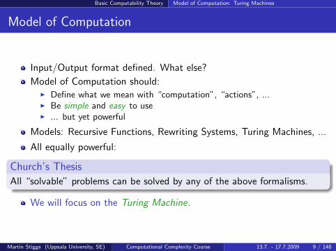
Input/Output format defined. What else?
Model of Computation should:I Define what we mean with “computation”, “actions”, ...I Be simple and easy to useI ... but yet powerful
Models: Recursive Functions, Rewriting Systems, Turing Machines, ...
All equally powerful:
Church’s Thesis
All “solvable” problems can be solved by any of the above formalisms.
We will focus on the Turing Machine.
Martin Stigge (Uppsala University, SE) Computational Complexity Course 13.7. - 17.7.2009 9 / 148
Basic Computability Theory Model of Computation: Turing Machines
Turing Machine
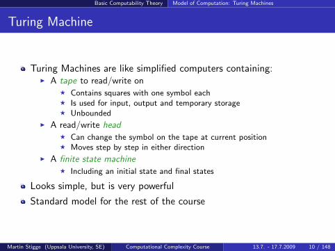
Turing Machines are like simplified computers containing:I A tape to read/write on
F Contains squares with one symbol eachF Is used for input, output and temporary storageF Unbounded
I A read/write headF Can change the symbol on the tape at current positionF Moves step by step in either direction
I A finite state machineF Including an initial state and final states
Looks simple, but is very powerful
Standard model for the rest of the course
Martin Stigge (Uppsala University, SE) Computational Complexity Course 13.7. - 17.7.2009 10 / 148
Basic Computability Theory Model of Computation: Turing Machines
Turing Machine: Definition
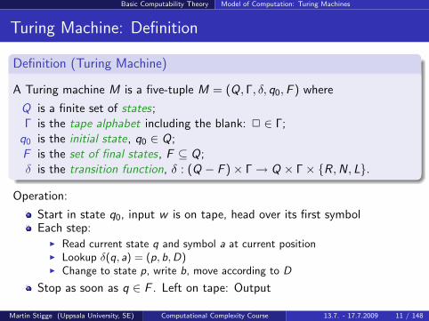
Definition (Turing Machine)
A Turing machine M is a five-tuple M = (Q, Γ, δ, q0,F ) where
Q is a finite set of states;Γ is the tape alphabet including the blank: 2 ∈ Γ;
q0 is the initial state, q0 ∈ Q;F is the set of final states, F ⊆ Q;δ is the transition function, δ : (Q − F )× Γ→ Q × Γ× R,N, L.
Operation:
Start in state q0, input w is on tape, head over its first symbolEach step:
I Read current state q and symbol a at current positionI Lookup δ(q, a) = (p, b,D)I Change to state p, write b, move according to D
Stop as soon as q ∈ F . Left on tape: Output
Martin Stigge (Uppsala University, SE) Computational Complexity Course 13.7. - 17.7.2009 11 / 148
Basic Computability Theory Model of Computation: Turing Machines
Turing Machine: Configuration
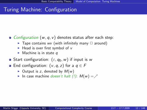
Configuration (w , q, v) denotes status after each step:I Tape contains wv (with infinitely many 2 around)I Head is over first symbol of vI Machine is in state q
Start configuration: (ε, q0,w) if input is w
End configuration: (v , q, z) for a q ∈ FI Output is z , denoted by M(w)I In case machine doesn’t halt (!): M(w) =
Martin Stigge (Uppsala University, SE) Computational Complexity Course 13.7. - 17.7.2009 12 / 148
Basic Computability Theory Model of Computation: Turing Machines
Turing Machine: Step Relation
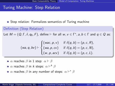
Step relation: Formalizes semantics of Turing machine
Definition (Step Relation)
Let M = (Q, Γ, δ, q0,F ), define ` for all w , v ∈ Γ∗, a, b ∈ Γ and q ∈ Q as:
(wa, q, bv) `
(wac , p, v) if δ(q, b) = (p, c,R),
(wa, p, cv) if δ(q, b) = (p, c,N),
(w , p, acv) if δ(q, b) = (p, c, L).
α reaches β in 1 step: α ` βα reaches β in k steps: α `k β
α reaches β in any number of steps: α `∗ β
Martin Stigge (Uppsala University, SE) Computational Complexity Course 13.7. - 17.7.2009 13 / 148
Basic Computability Theory Model of Computation: Turing Machines
Turing Machine: The Universal Machine
Turing machine model is quite simple
Can be easily simulated by a humanI Provided enough pencils, tape space and patience
Important result: Machines can simulate machinesI Turing machines are finite objects!I Effective encoding into words over an alphabetI Also configurations are finite! Encode them also
Simulator machine U only needs toI Receive an encoded M as inputI Input of M is w , give that also to UI U maintains encoded configurations of M and applies steps
Martin Stigge (Uppsala University, SE) Computational Complexity Course 13.7. - 17.7.2009 14 / 148
Basic Computability Theory Model of Computation: Turing Machines
Turing Machine: The Universal Machine (Cont.)
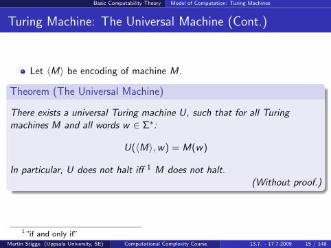
Let 〈M〉 be encoding of machine M.
Theorem (The Universal Machine)
There exists a universal Turing machine U, such that for all Turingmachines M and all words w ∈ Σ∗:
U(〈M〉,w) = M(w)
In particular, U does not halt iff 1 M does not halt.(Without proof.)
1“if and only if”Martin Stigge (Uppsala University, SE) Computational Complexity Course 13.7. - 17.7.2009 15 / 148
Basic Computability Theory Model of Computation: Turing Machines
Turing Machine: Transducers and Acceptors
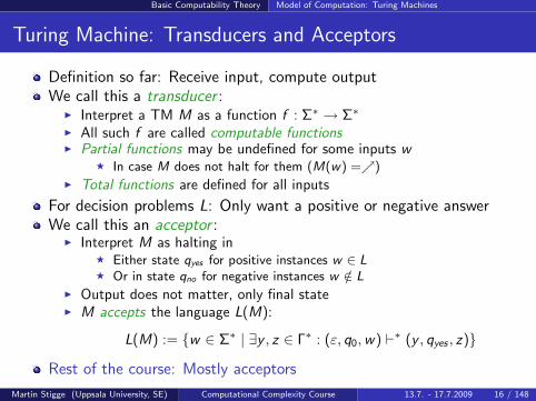
Definition so far: Receive input, compute outputWe call this a transducer :
I Interpret a TM M as a function f : Σ∗ → Σ∗
I All such f are called computable functionsI Partial functions may be undefined for some inputs w
F In case M does not halt for them (M(w) =)I Total functions are defined for all inputs
For decision problems L: Only want a positive or negative answerWe call this an acceptor :
I Interpret M as halting inF Either state qyes for positive instances w ∈ LF Or in state qno for negative instances w /∈ L
I Output does not matter, only final stateI M accepts the language L(M):
L(M) := w ∈ Σ∗ | ∃y , z ∈ Γ∗ : (ε, q0,w) `∗ (y , qyes , z)
Rest of the course: Mostly acceptors
Martin Stigge (Uppsala University, SE) Computational Complexity Course 13.7. - 17.7.2009 16 / 148
Basic Computability Theory Model of Computation: Turing Machines
Turing Machine: Multiple Tapes
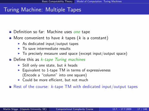
Definition so far: Machine uses one tape
More convenient to have k tapes (k is a constant)I As dedicated input/output tapesI To save intermediate resultsI To precisely measure used space (except input/output space)
Define this as k-tape Turing machinesI Still only one state, but k headsI Equivalent to 1-tape TM in terms of expressiveness
(Encode a “column” into one square)I Could be more efficient, but not much
Rest of the course: k-tape TM with dedicated input/output tapes
Martin Stigge (Uppsala University, SE) Computational Complexity Course 13.7. - 17.7.2009 17 / 148
Basic Computability Theory Model of Computation: Turing Machines
Turing Machine: Non-determinism
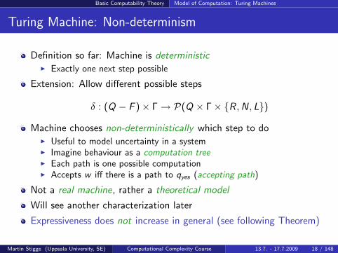
Definition so far: Machine is deterministicI Exactly one next step possible
Extension: Allow different possible steps
δ : (Q − F )× Γ→ P(Q × Γ× R,N, L)
Machine chooses non-deterministically which step to doI Useful to model uncertainty in a systemI Imagine behaviour as a computation treeI Each path is one possible computationI Accepts w iff there is a path to qyes (accepting path)
Not a real machine, rather a theoretical model
Will see another characterization later
Expressiveness does not increase in general (see following Theorem)
Martin Stigge (Uppsala University, SE) Computational Complexity Course 13.7. - 17.7.2009 18 / 148
Basic Computability Theory Model of Computation: Turing Machines
Turing Machine: Non-determinism (Cont.)
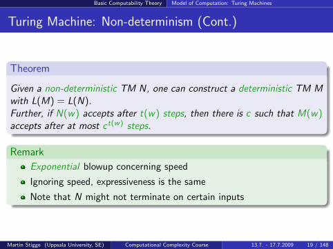
Theorem
Given a non-deterministic TM N, one can construct a deterministic TM Mwith L(M) = L(N).Further, if N(w) accepts after t(w) steps, then there is c such that M(w)accepts after at most ct(w) steps.
Remark
Exponential blowup concerning speed
Ignoring speed, expressiveness is the same
Note that N might not terminate on certain inputs
Martin Stigge (Uppsala University, SE) Computational Complexity Course 13.7. - 17.7.2009 19 / 148
Basic Computability Theory Model of Computation: Turing Machines
Turing Machine: Non-determinism (Cont. 2)
Proof (Sketch).
Given a non-deterministic N and an input w
Search the computation tree of N
Breadth-first technique: Visit all “early” configurations firstI Since there may be infinite pathsI For each i ≥ 0, visit all configurations up to depth iI If N accepts w , we will find accepting configuration at a depth t and
halt in qyes
I If N rejects w , we halt in qno or don’t terminate
Let d be maximal degree of non-determinism (choices of δ)
Above takes at most∑t
i=0 d i steps
Can be bounded from above by ct with a suitable constant c
Martin Stigge (Uppsala University, SE) Computational Complexity Course 13.7. - 17.7.2009 20 / 148
Basic Computability Theory Model of Computation: Turing Machines
Summary (Turing Machine)
Simple model of computation, but powerful
Clearly defined syntax and semantics
May accept languages or compute functions
May use multiple tapes
Non-determinism does not increase expressiveness
A Universal Machine exists, simulating all other machines
Remark
The machines we use from now on
are deterministic
are acceptors,
with k tapes
(except stated otherwise).
Martin Stigge (Uppsala University, SE) Computational Complexity Course 13.7. - 17.7.2009 21 / 148
Basic Computability Theory Decidability, Undecidability, Semi-Decidability
Deciding a Problem
Recall: Turing Machines running with input w mayI halt in state qyes ,I halt in state qno , orI run without halting .
Given problem L and instance w , want to decide whether w ∈ L:I Using a machine MI If w ∈ L, M should halt in qyes
I If w /∈ L, M should halt in qno
In particular: Always terminate! (Little use otherwise...)
Martin Stigge (Uppsala University, SE) Computational Complexity Course 13.7. - 17.7.2009 22 / 148
Basic Computability Theory Decidability, Undecidability, Semi-Decidability
Decidability and Undecidability
Definition
L is called decidable, if there exists a TM M with L(M) = L thathalts on all inputs.REC is the set of all decidable languages.
We can decide the status of w by just running M(w).
Termination guaranteed, we won’t wait infinitely
“M decides L”
If L /∈ REC, then L is undecidable
Martin Stigge (Uppsala University, SE) Computational Complexity Course 13.7. - 17.7.2009 23 / 148
Basic Computability Theory Decidability, Undecidability, Semi-Decidability
Decidability and Undecidability: Example
Example (PRIMES ∈ REC)
Recall PRIMES := [p]10 | p is a prime numberCan be decided:
I Given w = [n]10 for some nI Check for all i ∈ (1, n) whether n is multiple of iI If an i found: Halt in qno
I Otherwise, if all i negative: Halt in qyes
Can be implemented with a Turing machine
Always terminates (only finitely many i)
Thus: PRIMES ∈ REC
Martin Stigge (Uppsala University, SE) Computational Complexity Course 13.7. - 17.7.2009 24 / 148
Basic Computability Theory Decidability, Undecidability, Semi-Decidability
Semi-Decidability
Definition
L is called semi-decidable, if there exists a TM M with L(M) = L.RE is the set of all semi-decidable languages.
Note the missing “halts on all inputs”!
We can only “half-decide” the status of a given w :I Run M, wait for answerI If w ∈ L, M will halt in qyes
I If w /∈ L, M may not haltI We don’t know: w /∈ L or too impatient?
“M semi-decides L”
Martin Stigge (Uppsala University, SE) Computational Complexity Course 13.7. - 17.7.2009 25 / 148
Basic Computability Theory Decidability, Undecidability, Semi-Decidability
Class Differences
Questions at this point:1 Are there undecidable problems?2 Can we at least semi-decide some of them?3 Are there any we can’t even semi-decide?
Formally: REC?( RE
?( P(Σ∗)
Subtle difference between REC and RE: Termination guarantee
Martin Stigge (Uppsala University, SE) Computational Complexity Course 13.7. - 17.7.2009 26 / 148
Basic Computability Theory Decidability, Undecidability, Semi-Decidability
Properties of Complementation
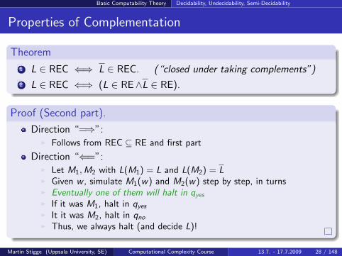
Theorem
1 L ∈ REC ⇐⇒ L ∈ REC. (“closed under taking complements”)
2 L ∈ REC ⇐⇒ (L ∈ RE∧L ∈ RE).
Proof (First part).
Direction “=⇒”:I Assume M decides L and halts alwaysI Construct M ′: Like M, but swap qyes and qno
I M ′ decides L and halts always!
Direction “⇐=”:I Exact same thing.
Martin Stigge (Uppsala University, SE) Computational Complexity Course 13.7. - 17.7.2009 27 / 148
Basic Computability Theory Decidability, Undecidability, Semi-Decidability
Properties of Complementation
Theorem
1 L ∈ REC ⇐⇒ L ∈ REC. (“closed under taking complements”)
2 L ∈ REC ⇐⇒ (L ∈ RE∧L ∈ RE).
Proof (Second part).
Direction “=⇒”:I Follows from REC ⊆ RE and first part
Direction “⇐=”:I Let M1,M2 with L(M1) = L and L(M2) = LI Given w , simulate M1(w) and M2(w) step by step, in turnsI Eventually one of them will halt in qyes
I If it was M1, halt in qyes
I It it was M2, halt in qno
I Thus, we always halt (and decide L)!
Martin Stigge (Uppsala University, SE) Computational Complexity Course 13.7. - 17.7.2009 28 / 148
Basic Computability Theory Decidability, Undecidability, Semi-Decidability
The Halting Problem
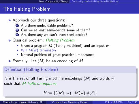
Approach our three questions:1 Are there undecidable problems?2 Can we at least semi-decide some of them?3 Are there any we can’t even semi-decide?
Classical problem: Halting ProblemI Given a program M (Turing machine!) and an input wI Will M(w) terminate?I Natural problem of great practical importance
Formally: Let 〈M〉 be an encoding of M
Definition (Halting Problem)
H is the set of all Turing machine encodings 〈M〉 and words w ,such that M halts on input w :
H := (〈M〉,w) | M(w) 6=
Martin Stigge (Uppsala University, SE) Computational Complexity Course 13.7. - 17.7.2009 29 / 148
Basic Computability Theory Decidability, Undecidability, Semi-Decidability
Undecidability of the Halting Problem
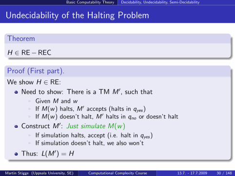
Theorem
H ∈ RE−REC
Proof (First part).
We show H ∈ RE:
Need to show: There is a TM M ′, such thatI Given M and wI If M(w) halts, M ′ accepts (halts in qyes)I If M(w) doesn’t halt, M ′ halts in qno or doesn’t halt
Construct M ′: Just simulate M(w)I If simulation halts, accept (i.e. halt in qyes)I If simulation doesn’t halt, we also won’t
Thus: L(M ′) = H
Martin Stigge (Uppsala University, SE) Computational Complexity Course 13.7. - 17.7.2009 30 / 148
Basic Computability Theory Decidability, Undecidability, Semi-Decidability
Undecidability of the Halting Problem (Cont.)
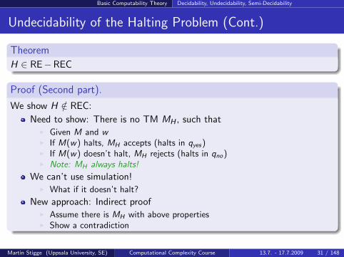
Theorem
H ∈ RE−REC
Proof (Second part).
We show H /∈ REC:
Need to show: There is no TM MH , such thatI Given M and wI If M(w) halts, MH accepts (halts in qyes)I If M(w) doesn’t halt, MH rejects (halts in qno)I Note: MH always halts!
We can’t use simulation!I What if it doesn’t halt?
New approach: Indirect proofI Assume there is MH with above propertiesI Show a contradiction
Martin Stigge (Uppsala University, SE) Computational Complexity Course 13.7. - 17.7.2009 31 / 148
Basic Computability Theory Decidability, Undecidability, Semi-Decidability
Undecidability of the Halting Problem (Cont. 2)
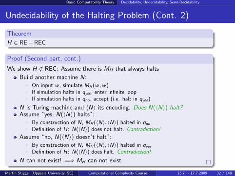
Theorem
H ∈ RE−REC
Proof (Second part, cont.)
We show H /∈ REC: Assume there is MH that always halts
Build another machine N:I On input w , simulate MH(w ,w)I If simulation halts in qyes , enter infinite loopI If simulation halts in qno , accept (i.e. halt in qyes)
N is Turing machine and 〈N〉 its encoding. Does N(〈N〉) halt?Assume “yes, N(〈N〉) halts”:
I By construction of N, MH(〈N〉, 〈N〉) halted in qno
I Definition of H: N(〈N〉) does not halt. Contradiction!
Assume “no, N(〈N〉) doesn’t halt”:I By construction of N, MH(〈N〉, 〈N〉) halted in qyes
I Definition of H: N(〈N〉) does halt. Contradiction!
N can not exist! =⇒ MH can not exist.
Martin Stigge (Uppsala University, SE) Computational Complexity Course 13.7. - 17.7.2009 32 / 148
Basic Computability Theory Decidability, Undecidability, Semi-Decidability
Class Differences: Results
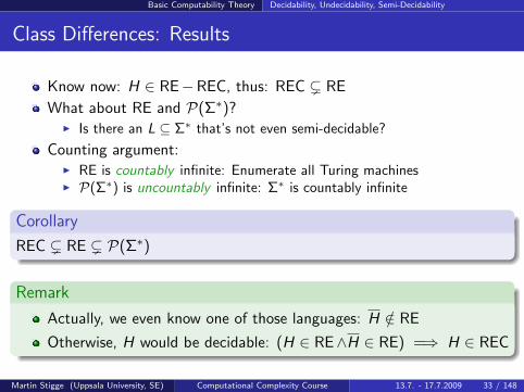
Know now: H ∈ RE−REC, thus: REC ( RE
What about RE and P(Σ∗)?I Is there an L ⊆ Σ∗ that’s not even semi-decidable?
Counting argument:I RE is countably infinite: Enumerate all Turing machinesI P(Σ∗) is uncountably infinite: Σ∗ is countably infinite
Corollary
REC ( RE ( P(Σ∗)
Remark
Actually, we even know one of those languages: H /∈ RE
Otherwise, H would be decidable: (H ∈ RE∧H ∈ RE) =⇒ H ∈ REC
Martin Stigge (Uppsala University, SE) Computational Complexity Course 13.7. - 17.7.2009 33 / 148
Basic Computability Theory Decidability, Undecidability, Semi-Decidability
Reductions
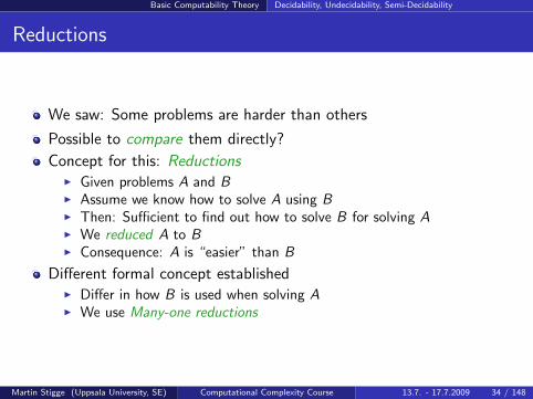
We saw: Some problems are harder than others
Possible to compare them directly?
Concept for this: ReductionsI Given problems A and BI Assume we know how to solve A using BI Then: Sufficient to find out how to solve B for solving AI We reduced A to BI Consequence: A is “easier” than B
Different formal concept establishedI Differ in how B is used when solving AI We use Many-one reductions
Martin Stigge (Uppsala University, SE) Computational Complexity Course 13.7. - 17.7.2009 34 / 148
Basic Computability Theory Decidability, Undecidability, Semi-Decidability
Reductions: Definition
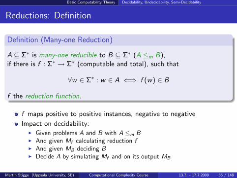
Definition (Many-one Reduction)
A ⊆ Σ∗ is many-one reducible to B ⊆ Σ∗ (A ≤m B),if there is f : Σ∗ → Σ∗ (computable and total), such that
∀w ∈ Σ∗ : w ∈ A ⇐⇒ f (w) ∈ B
f the reduction function.
f maps positive to positive instances, negative to negative
Impact on decidability:I Given problems A and B with A ≤m BI And given Mf calculating reduction fI And given MB deciding BI Decide A by simulating Mf and on its output MB
Martin Stigge (Uppsala University, SE) Computational Complexity Course 13.7. - 17.7.2009 35 / 148
Basic Computability Theory Decidability, Undecidability, Semi-Decidability
Reductions: Properties
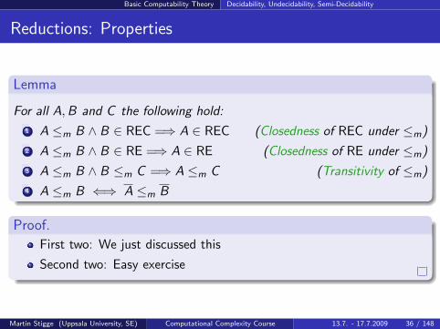
Lemma
For all A,B and C the following hold:
1 A ≤m B ∧ B ∈ REC =⇒ A ∈ REC (Closedness of REC under ≤m)
2 A ≤m B ∧ B ∈ RE =⇒ A ∈ RE (Closedness of RE under ≤m)
3 A ≤m B ∧ B ≤m C =⇒ A ≤m C (Transitivity of ≤m)
4 A ≤m B ⇐⇒ A ≤m B
Proof.
First two: We just discussed this
Second two: Easy exercise
Martin Stigge (Uppsala University, SE) Computational Complexity Course 13.7. - 17.7.2009 36 / 148
Basic Computability Theory Decidability, Undecidability, Semi-Decidability
Reductions: Example
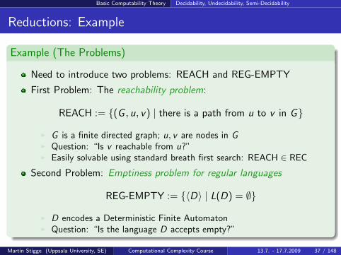
Example (The Problems)
Need to introduce two problems: REACH and REG-EMPTY
First Problem: The reachability problem:
REACH := (G , u, v) | there is a path from u to v in G
I G is a finite directed graph; u, v are nodes in GI Question: “Is v reachable from u?”I Easily solvable using standard breath first search: REACH ∈ REC
Second Problem: Emptiness problem for regular languages
REG-EMPTY := 〈D〉 | L(D) = ∅
I D encodes a Deterministic Finite AutomatonI Question: “Is the language D accepts empty?”
Martin Stigge (Uppsala University, SE) Computational Complexity Course 13.7. - 17.7.2009 37 / 148
Basic Computability Theory Decidability, Undecidability, Semi-Decidability
Reductions: Example (Cont.)
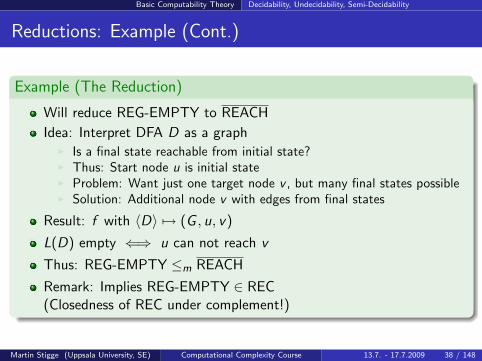
Example (The Reduction)
Will reduce REG-EMPTY to REACH
Idea: Interpret DFA D as a graphI Is a final state reachable from initial state?I Thus: Start node u is initial stateI Problem: Want just one target node v , but many final states possibleI Solution: Additional node v with edges from final states
Result: f with 〈D〉 7→ (G , u, v)
L(D) empty ⇐⇒ u can not reach v
Thus: REG-EMPTY ≤m REACH
Remark: Implies REG-EMPTY ∈ REC(Closedness of REC under complement!)
Martin Stigge (Uppsala University, SE) Computational Complexity Course 13.7. - 17.7.2009 38 / 148
Basic Computability Theory Decidability, Undecidability, Semi-Decidability
A Second Example: Halting Problem with empty input
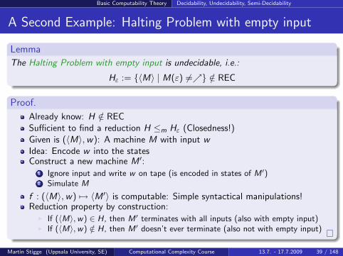
Lemma
The Halting Problem with empty input is undecidable, i.e.:
Hε := 〈M〉 | M(ε) 6= /∈ REC
Proof.
Already know: H /∈ RECSufficient to find a reduction H ≤m Hε (Closedness!)Given is (〈M〉,w): A machine M with input wIdea: Encode w into the statesConstruct a new machine M ′:
1 Ignore input and write w on tape (is encoded in states of M ′)2 Simulate M
f : (〈M〉,w) 7→ 〈M ′〉 is computable: Simple syntactical manipulations!Reduction property by construction:
I If (〈M〉,w) ∈ H, then M ′ terminates with all inputs (also with empty input)I If (〈M〉,w) /∈ H, then M ′ doesn’t ever terminate (also not with empty input)
Martin Stigge (Uppsala University, SE) Computational Complexity Course 13.7. - 17.7.2009 39 / 148
Basic Computability Theory Decidability, Undecidability, Semi-Decidability
Rice’s Theorem: Introduction
We know now: Halting is undecidable for Turing machines
Even for just empty input!
Are other properties undecidable?
(Maybe halting is just a strange property..)
Will see now: No “non-trivial” behavioural property is decidable!I For Turing machinesI Simpler models behave better (DFA..)I Non-trivial: Some Turing machines have it, some don’t
High practical relevance:I Either have to restrict model (less expressive)I Or only approximate answers (less precise)
Formally: Rice’s Theorem
Martin Stigge (Uppsala University, SE) Computational Complexity Course 13.7. - 17.7.2009 40 / 148
Basic Computability Theory Decidability, Undecidability, Semi-Decidability
Rice’s Theorem: Formal formulation
Theorem (Rice’s Theorem)
Let C be a non-trivial class of semi-decidable languages, i.e., ∅ ( C ( RE.Then the following LC is undecidable:
LC := 〈M〉 | L(M) ∈ C
Proof (Overview).
First assume ∅ /∈ CThen there must be a non-empty A ∈ C (since C is non-empty)We will reduce H to LCIdea:
I We are given M with input wI Simulate M(w)I If it halts, we will semi-decide AI If it doesn’t halt, we will semi-decide ∅ (never accept)I This is the reduction!
Martin Stigge (Uppsala University, SE) Computational Complexity Course 13.7. - 17.7.2009 41 / 148
Basic Computability Theory Decidability, Undecidability, Semi-Decidability
Rice’s Theorem: Formal formulation (Cont.)
Theorem (Rice’s Theorem)
Let C be a non-trivial class of semi-decidable languages, i.e., ∅ ( C ( RE.Then the following LC is undecidable:
LC := 〈M〉 | L(M) ∈ C
Proof (Details).
Recall: ∅ /∈ C, A ∈ C, let MA be machine for AConstruct a new machine M ′:
1 Input y , first simulate M(w) on second tape2 If M(w) halts, simulate MA(y)
Reduction property by construction:I If (〈M〉,w) ∈ H, then L(M ′) = A, thus 〈M ′〉 ∈ LCI If (〈M〉,w) /∈ H, then L(M ′) = ∅, thus 〈M ′〉 /∈ LC
What about the case ∅ ∈ C? Similar construction showing H ≤m LC
Martin Stigge (Uppsala University, SE) Computational Complexity Course 13.7. - 17.7.2009 42 / 148
Basic Computability Theory Decidability, Undecidability, Semi-Decidability
Rice’s Theorem: Examples
Example
The following language is undecidable:
L := 〈M〉 | L(M) contains at most 5 words
Follows from Rice’s Theorem since C 6= ∅ and C 6= RE
Thus: For any k, can’t decide if an M only accepts at most k inputs
Example
The following language is decidable:
L := 〈M〉 | M contains at most 5 states
Easy check by looking at encoding of M
Not a behavioural property
Martin Stigge (Uppsala University, SE) Computational Complexity Course 13.7. - 17.7.2009 43 / 148
Basic Computability Theory Decidability, Undecidability, Semi-Decidability
Summary Computability Theory
Defined a model of computation: Turing machines
Explored properties:I Decidability and UndecidabilityI Semi-DecidabilityI Example: The Halting problem is undecidable
Reductions as a relative concept
Closedness allows using them for absolute results
Rice’s Theorem:All non-trivial behavioural properties of TM are undecidable.
Martin Stigge (Uppsala University, SE) Computational Complexity Course 13.7. - 17.7.2009 44 / 148
Complexity Classes
Course Outline
0 Introduction
1 Basic Computability TheoryFormal LanguagesModel of Computation: Turing MachinesDecidability, Undecidability, Semi-Decidability
2 Complexity ClassesLandau Symbols: The O(·) NotationTime and Space ComplexityRelations between Complexity Classes
3 Feasible Computations: P vs. NPProving vs. VerifyingReductions, Hardness, CompletenessNatural NP-complete problems
4 Advanced Complexity ConceptsNon-uniform ComplexityProbabilistic Complexity ClassesInteractive Proof Systems
Martin Stigge (Uppsala University, SE) Computational Complexity Course 13.7. - 17.7.2009 45 / 148
Complexity Classes Introduction
Restricted Resources
Previous Chapter: Computability TheoryI “What can algorithms do?”
Now: Complexity TheoryI “What can algorithms do with restricted resources?”I Resources: Runtime and memory
Assume the machines always halt in qyes or qno
I But after how many steps?I How many tape positions were necessary?
Martin Stigge (Uppsala University, SE) Computational Complexity Course 13.7. - 17.7.2009 46 / 148
Complexity Classes Landau Symbols
Landau Symbols
Resource bounds will depend on input size
Described by functions f : N→ NNeed ability to express “grows in the order of”
I Consider f1(n) = n2 and f2(n) = 5 · n2 + 3I Eventually, n2 dominates for large nI Both express “quadratic growth”I Want to see all c1 · n2 + c2 equivalentI Asymptotic behaviour
Formal notation for this: O(n2)
Will provide a kind of upper bound of asymptotic growth
Martin Stigge (Uppsala University, SE) Computational Complexity Course 13.7. - 17.7.2009 47 / 148
Complexity Classes Landau Symbols
Landau Symbols: Definition
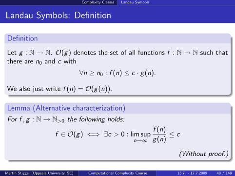
Definition
Let g : N→ N. O(g) denotes the set of all functions f : N→ N such thatthere are n0 and c with
∀n ≥ n0 : f (n) ≤ c · g(n).
We also just write f (n) = O(g(n)).
Lemma (Alternative characterization)
For f , g : N→ N>0 the following holds:
f ∈ O(g) ⇐⇒ ∃c > 0 : lim supn→∞
f (n)
g(n)≤ c
(Without proof.)
Martin Stigge (Uppsala University, SE) Computational Complexity Course 13.7. - 17.7.2009 48 / 148
Complexity Classes Landau Symbols
Landau Symbols: Examples
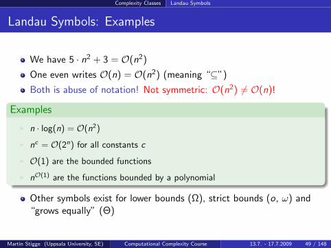
We have 5 · n2 + 3 = O(n2)
One even writes O(n) = O(n2) (meaning “⊆”)
Both is abuse of notation! Not symmetric: O(n2) 6= O(n)!
Examples
I n · log(n) = O(n2)
I nc = O(2n) for all constants c
I O(1) are the bounded functions
I nO(1) are the functions bounded by a polynomial
Other symbols exist for lower bounds (Ω), strict bounds (o, ω) and“grows equally” (Θ)
Martin Stigge (Uppsala University, SE) Computational Complexity Course 13.7. - 17.7.2009 49 / 148
Complexity Classes Time and Space Complexity
Proper complexity functions
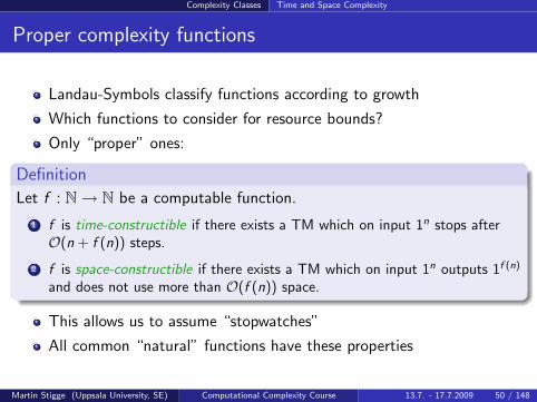
Landau-Symbols classify functions according to growth
Which functions to consider for resource bounds?
Only “proper” ones:
Definition
Let f : N→ N be a computable function.
1 f is time-constructible if there exists a TM which on input 1n stops afterO(n + f (n)) steps.
2 f is space-constructible if there exists a TM which on input 1n outputs 1f (n)
and does not use more than O(f (n)) space.
This allows us to assume “stopwatches”
All common “natural” functions have these properties
Martin Stigge (Uppsala University, SE) Computational Complexity Course 13.7. - 17.7.2009 50 / 148
Complexity Classes Time and Space Complexity
Resource measures
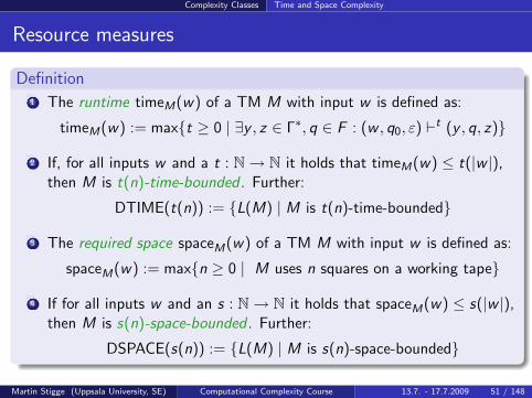
Definition1 The runtime timeM(w) of a TM M with input w is defined as:
timeM(w) := maxt ≥ 0 | ∃y , z ∈ Γ∗, q ∈ F : (w , q0, ε) `t (y , q, z)
2 If, for all inputs w and a t : N→ N it holds that timeM(w) ≤ t(|w |),then M is t(n)-time-bounded . Further:
DTIME(t(n)) := L(M) | M is t(n)-time-bounded
3 The required space spaceM(w) of a TM M with input w is defined as:
spaceM(w) := maxn ≥ 0 | M uses n squares on a working tape
4 If for all inputs w and an s : N→ N it holds that spaceM(w) ≤ s(|w |),then M is s(n)-space-bounded . Further:
DSPACE(s(n)) := L(M) | M is s(n)-space-bounded
Martin Stigge (Uppsala University, SE) Computational Complexity Course 13.7. - 17.7.2009 51 / 148
Complexity Classes Time and Space Complexity
Resource measures (Cont.)
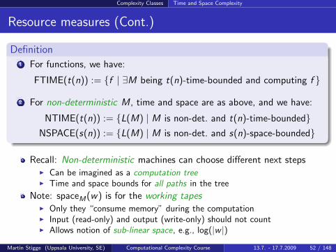
Definition1 For functions, we have:
FTIME(t(n)) := f | ∃M being t(n)-time-bounded and computing f
2 For non-deterministic M, time and space are as above, and we have:
NTIME(t(n)) := L(M) | M is non-det. and t(n)-time-boundedNSPACE(s(n)) := L(M) | M is non-det. and s(n)-space-bounded
Recall: Non-deterministic machines can choose different next stepsI Can be imagined as a computation treeI Time and space bounds for all paths in the tree
Note: spaceM(w) is for the working tapesI Only they “consume memory” during the computationI Input (read-only) and output (write-only) should not countI Allows notion of sub-linear space, e.g., log(|w |)
Martin Stigge (Uppsala University, SE) Computational Complexity Course 13.7. - 17.7.2009 52 / 148
Complexity Classes Time and Space Complexity
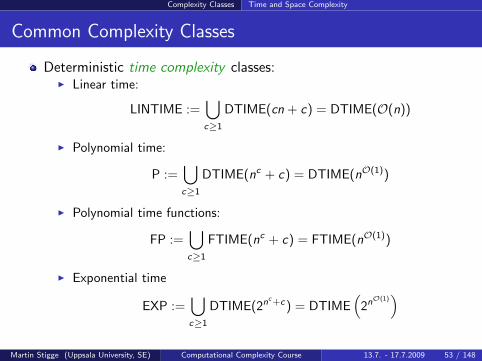
Common Complexity Classes
Deterministic time complexity classes:I Linear time:
LINTIME :=⋃c≥1
DTIME(cn + c) = DTIME(O(n))
I Polynomial time:
P :=⋃c≥1
DTIME(nc + c) = DTIME(nO(1))
I Polynomial time functions:
FP :=⋃c≥1
FTIME(nc + c) = FTIME(nO(1))
I Exponential time
EXP :=⋃c≥1
DTIME(2nc +c) = DTIME(
2nO(1))
Martin Stigge (Uppsala University, SE) Computational Complexity Course 13.7. - 17.7.2009 53 / 148
Complexity Classes Time and Space Complexity
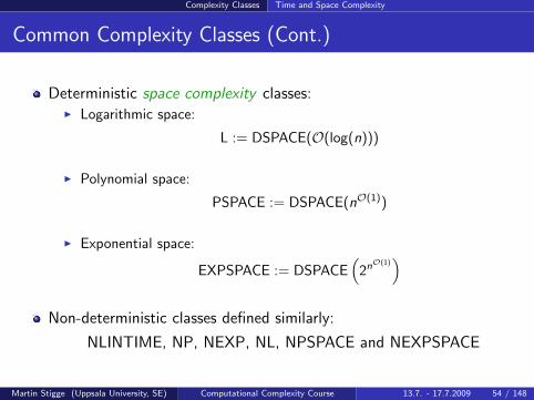
Common Complexity Classes (Cont.)
Deterministic space complexity classes:I Logarithmic space:
L := DSPACE(O(log(n)))
I Polynomial space:
PSPACE := DSPACE(nO(1))
I Exponential space:
EXPSPACE := DSPACE(
2nO(1))
Non-deterministic classes defined similarly:
NLINTIME, NP, NEXP, NL, NPSPACE and NEXPSPACE
Martin Stigge (Uppsala University, SE) Computational Complexity Course 13.7. - 17.7.2009 54 / 148
Complexity Classes Time and Space Complexity
Common Complexity Classes: Example
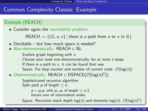
Example (REACH)
Consider again the reachability problem:
REACH := (G , u, v) | there is a path from u to v in GDecidable – but how much space is needed?Non-deterministically : REACH ∈ NL
I Explore graph beginning with uI Choose next node non-deterministically, for at most n stepsI If there is a path to v , it can be found that wayI Space: For step counter and number of current node: O(log(n))
Deterministically : REACH ∈ DSPACE(O(log(n)2))I Sophisticated recursive algorithmI Split path p of length ≤ n:
F p = p1p2 with p1, p2 of length ≤ n/2F Iterate over all intermediate nodes
I Space: Recursion stack depth log(n) and elements log(n): O(log(n)2)
Martin Stigge (Uppsala University, SE) Computational Complexity Course 13.7. - 17.7.2009 55 / 148
Complexity Classes Relations between Complexity Classes
Complexity Class Relations
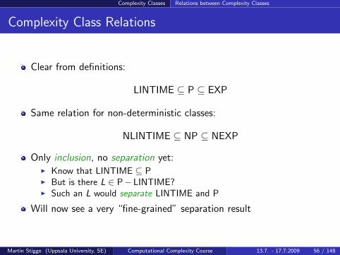
Clear from definitions:
LINTIME ⊆ P ⊆ EXP
Same relation for non-deterministic classes:
NLINTIME ⊆ NP ⊆ NEXP
Only inclusion, no separation yet:I Know that LINTIME ⊆ PI But is there L ∈ P− LINTIME?I Such an L would separate LINTIME and P
Will now see a very “fine-grained” separation result
Martin Stigge (Uppsala University, SE) Computational Complexity Course 13.7. - 17.7.2009 56 / 148
Complexity Classes Relations between Complexity Classes
Hierarchy Theorem
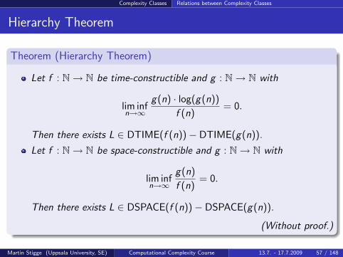
Theorem (Hierarchy Theorem)
Let f : N→ N be time-constructible and g : N→ N with
lim infn→∞
g(n) · log(g(n))
f (n)= 0.
Then there exists L ∈ DTIME(f (n))− DTIME(g(n)).
Let f : N→ N be space-constructible and g : N→ N with
lim infn→∞
g(n)
f (n)= 0.
Then there exists L ∈ DSPACE(f (n))− DSPACE(g(n)).
(Without proof.)
Martin Stigge (Uppsala University, SE) Computational Complexity Course 13.7. - 17.7.2009 57 / 148
Complexity Classes Relations between Complexity Classes
Hierarchy Theorem: Examples
Example
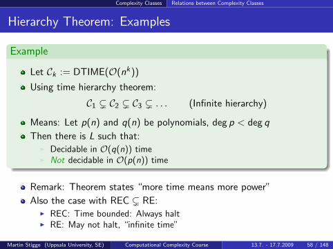
Let Ck := DTIME(O(nk))
Using time hierarchy theorem:
C1 ( C2 ( C3 ( . . . (Infinite hierarchy)
Means: Let p(n) and q(n) be polynomials, deg p < deg q
Then there is L such that:I Decidable in O(q(n)) timeI Not decidable in O(p(n)) time
Remark: Theorem states “more time means more power”
Also the case with REC ( RE:I REC: Time bounded: Always haltI RE: May not halt, “infinite time”
Martin Stigge (Uppsala University, SE) Computational Complexity Course 13.7. - 17.7.2009 58 / 148
Complexity Classes Relations between Complexity Classes
Determinism vs. Non-determinism
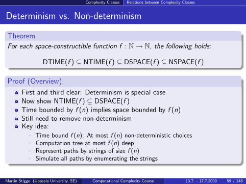
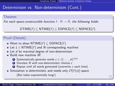
Theorem
For each space-constructible function f : N→ N, the following holds:
DTIME(f ) ⊆ NTIME(f ) ⊆ DSPACE(f ) ⊆ NSPACE(f )
Proof (Overview).
First and third clear: Determinism is special caseNow show NTIME(f ) ⊆ DSPACE(f )Time bounded by f (n) implies space bounded by f (n)Still need to remove non-determinismKey idea:
I Time bound f (n): At most f (n) non-deterministic choicesI Computation tree at most f (n) deepI Represent paths by strings of size f (n)I Simulate all paths by enumerating the strings
Martin Stigge (Uppsala University, SE) Computational Complexity Course 13.7. - 17.7.2009 59 / 148
Complexity Classes Relations between Complexity Classes
Determinism vs. Non-determinism (Cont.)
Theorem
For each space-constructible function f : N→ N, the following holds:
DTIME(f ) ⊆ NTIME(f ) ⊆ DSPACE(f ) ⊆ NSPACE(f )
Proof (Details).
Want to show NTIME(f ) ⊆ DSPACE(f )Let L ∈ NTIME(f ) and N corresponding machineLet d be maximal degree of non-determinismBuild new machine M:
1 Systematically generate words c ∈ 1, . . . , df (n)
2 Simulate N with non-deterministic choices c3 Repeat until all words generated (overwrite c each time)
Simulation is deterministic and needs only O(f (n)) spaceI (But takes exponentially long!)
Martin Stigge (Uppsala University, SE) Computational Complexity Course 13.7. - 17.7.2009 60 / 148
Complexity Classes Relations between Complexity Classes
Deterministic vs. Non-deterministic Space
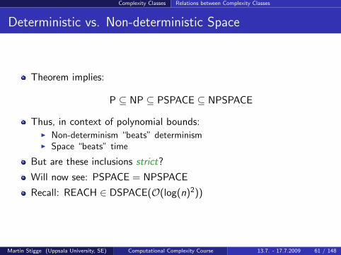
Theorem implies:
P ⊆ NP ⊆ PSPACE ⊆ NPSPACE
Thus, in context of polynomial bounds:I Non-determinism “beats” determinismI Space “beats” time
But are these inclusions strict?
Will now see: PSPACE = NPSPACE
Recall: REACH ∈ DSPACE(O(log(n)2))
Martin Stigge (Uppsala University, SE) Computational Complexity Course 13.7. - 17.7.2009 61 / 148
Complexity Classes Relations between Complexity Classes
Deterministic vs. Non-deterministic Space (Cont.)
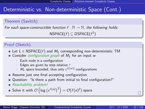
Theorem (Savitch)
For each space-constructible function f : N→ N, the following holds:
NSPACE(f ) ⊆ DSPACE(f 2)
Proof (Sketch).
Let L ∈ NSPACE(f ) and ML corresponding non-deterministic TMConsider configuration graph of ML for an input w
I Each node is a configurationI Edges are given by step relation `I ML space bounded, thus only c f (|w |) configurations
Assume just one final accepting configurationQuestion: “Is there a path from initial to final configuration?”Reachability problem!
Solve it with O(
log(c f (n)
)2)
= O(f (n)2) space
Martin Stigge (Uppsala University, SE) Computational Complexity Course 13.7. - 17.7.2009 62 / 148
Complexity Classes Relations between Complexity Classes
Polynomial Complexity Classes
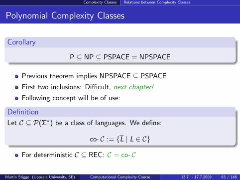
Corollary
P ⊆ NP ⊆ PSPACE = NPSPACE
Previous theorem implies NPSPACE ⊆ PSPACE
First two inclusions: Difficult, next chapter!
Following concept will be of use:
Definition
Let C ⊆ P(Σ∗) be a class of languages. We define:
co- C := L | L ∈ C
For deterministic C ⊆ REC: C = co- C
Martin Stigge (Uppsala University, SE) Computational Complexity Course 13.7. - 17.7.2009 63 / 148
Complexity Classes Relations between Complexity Classes
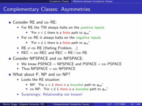
Complementary Classes: Asymmetries
Consider RE and co- RE:I For RE the TM always halts on the positive inputs
F “For x ∈ L there is a finite path to qyes”
I For co- RE it always halts on the negative inputsF “For x /∈ L there is a finite path to qno”
I RE 6= co- RE (Halting Problem, ..)I REC = co- REC and REC = RE∩ co- RE
Consider NPSPACE and co- NPSPACE:I We know PSPACE = NPSPACE and PSPACE = co- PSPACEI Thus NPSPACE = co- NPSPACE
What about P, NP and co- NP?I Looks like RE situation:
F NP: “For x ∈ L there is a bounded path to qyes”F co- NP: “For x /∈ L there is a bounded path to qno”
I Surprisingly: Relationship not known!
Martin Stigge (Uppsala University, SE) Computational Complexity Course 13.7. - 17.7.2009 64 / 148
Feasible Computations: P vs. NP Introduction
Course Outline
0 Introduction
1 Basic Computability TheoryFormal LanguagesModel of Computation: Turing MachinesDecidability, Undecidability, Semi-Decidability
2 Complexity ClassesLandau Symbols: The O(·) NotationTime and Space ComplexityRelations between Complexity Classes
3 Feasible Computations: P vs. NPProving vs. VerifyingReductions, Hardness, CompletenessNatural NP-complete problems
4 Advanced Complexity ConceptsNon-uniform ComplexityProbabilistic Complexity ClassesInteractive Proof Systems
Martin Stigge (Uppsala University, SE) Computational Complexity Course 13.7. - 17.7.2009 65 / 148
Feasible Computations: P vs. NP Introduction
Course Outline
0 Introduction
1 Basic Computability TheoryFormal LanguagesModel of Computation: Turing MachinesDecidability, Undecidability, Semi-Decidability
2 Complexity ClassesLandau Symbols: The O(·) NotationTime and Space ComplexityRelations between Complexity Classes
3 Feasible Computations: P vs. NPProving vs. VerifyingReductions, Hardness, CompletenessNatural NP-complete problems
4 Advanced Complexity ConceptsNon-uniform ComplexityProbabilistic Complexity ClassesInteractive Proof Systems
Martin Stigge (Uppsala University, SE) Computational Complexity Course 13.7. - 17.7.2009 66 / 148
Feasible Computations: P vs. NP Introduction
Feasible Computations
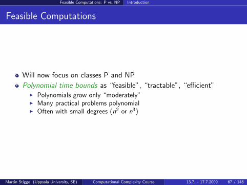
Will now focus on classes P and NP
Polynomial time bounds as “feasible”, “tractable”, “efficient”I Polynomials grow only “moderately”I Many practical problems polynomialI Often with small degrees (n2 or n3)
Martin Stigge (Uppsala University, SE) Computational Complexity Course 13.7. - 17.7.2009 67 / 148
Feasible Computations: P vs. NP Proving vs. Verifying
Recall P and NP
Introduced P and NP via Turing machines:I Polynomial time boundsI Deterministic vs. non-deterministic operation
Recall P: For L1 ∈ PI Existence of a deterministic TM MI Existence of a polynomial pM(n)I For each input x ∈ Σ∗ runtime ≤ pM(|x |)
Recall NP: For L2 ∈ NPI Existence of a non-deterministic TM NI Existence of a polynomial pN(n)I For each input x ∈ Σ∗ runtime ≤ pN(|x |)I For all computation paths
Theoretical model – practical significance?
Introduce now a new characterization of NP
Martin Stigge (Uppsala University, SE) Computational Complexity Course 13.7. - 17.7.2009 68 / 148
Feasible Computations: P vs. NP Proving vs. Verifying
A new NP characterization
Definition
Let R ∈ Σ∗ × Σ∗ (binary relation). R is polynomially bounded , if thereexists a polynomial p(n), such that:
∀(x , y) ∈ R : |y | ≤ p(|x |)
Lemma
NP is the class of all L such that there exists a polynomially boundedRL ∈ Σ∗ × Σ∗ satisfying:
RL ∈ P, and
x ∈ L ⇐⇒ ∃w : (x ,w) ∈ RL.
We call w a witness (or proof) for x ∈ L and RL the witness relation.
Martin Stigge (Uppsala University, SE) Computational Complexity Course 13.7. - 17.7.2009 69 / 148
Feasible Computations: P vs. NP Proving vs. Verifying
Proving vs. Verifying
For L ∈ P:I Machine must decide membership of x in polynomial timeI Interpret as “finding a proof ” for x ∈ L
For L ∈ NP: (new characterization)I Machine is provided a witness wI Interpret as “verifying the proof ” for x ∈ L
Efficient proving and verifying procedures:I For P, runtime is boundedI For NP, also witness size is bounded
Write L ∈ NP as:
L = x ∈ Σ∗ | ∃w ∈ Σ∗ : (x ,w) ∈ RL
Martin Stigge (Uppsala University, SE) Computational Complexity Course 13.7. - 17.7.2009 70 / 148
Feasible Computations: P vs. NP Proving vs. Verifying
Proving vs. Verifying (Cont.)
P-problems: solutions can be efficiently found
NP-problems: solutions can be efficiently checked
Checking certainly a prerequisite for finding (thus P ⊆ NP)
But is finding more difficult?I Intuition says: “Yes!”I Theory says: “We don’t know.” (yet?)
Formal formulation:P
?= NP
One of the most important questions of computer science!I Many proofs for either “=” or “ 6=”I None correct so farI Clay Mathematics Institute offers $1.000.000 prize
Martin Stigge (Uppsala University, SE) Computational Complexity Course 13.7. - 17.7.2009 71 / 148
Feasible Computations: P vs. NP Proving vs. Verifying
A new NP characterization (Cont.)
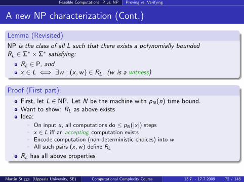
Lemma (Revisited)
NP is the class of all L such that there exists a polynomially boundedRL ∈ Σ∗ × Σ∗ satisfying:
RL ∈ P, andx ∈ L ⇐⇒ ∃w : (x ,w) ∈ RL. (w is a witness)
Proof (First part).
First, let L ∈ NP. Let N be the machine with pN(n) time bound.Want to show: RL as above existsIdea:
I On input x , all computations do ≤ pN(|x |) stepsI x ∈ L iff an accepting computation existsI Encode computation (non-deterministic choices) into wI All such pairs (x ,w) define RL
RL has all above properties
Martin Stigge (Uppsala University, SE) Computational Complexity Course 13.7. - 17.7.2009 72 / 148
Feasible Computations: P vs. NP Proving vs. Verifying
A new NP characterization (Cont. 2)
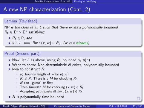
Lemma (Revisited)
NP is the class of all L such that there exists a polynomially boundedRL ∈ Σ∗ × Σ∗ satisfying:
RL ∈ P, andx ∈ L ⇐⇒ ∃w : (x ,w) ∈ RL. (w is a witness)
Proof (Second part).
Now, let L as above, using RL bounded by p(n)Want to show: Non-deterministic N exists, polynomially boundedIdea to construct N:
I RL bounds length of w by p(|x |)I RL ∈ P: There is a M for checking RL
I N can “guess” w firstI Then simulate M for checking (x ,w) ∈ RL
I Accepting path exists iff ∃w : (x ,w) ∈ RL
N is polynomially time bounded
Martin Stigge (Uppsala University, SE) Computational Complexity Course 13.7. - 17.7.2009 73 / 148
Feasible Computations: P vs. NP Proving vs. Verifying
A new co- NP characterization
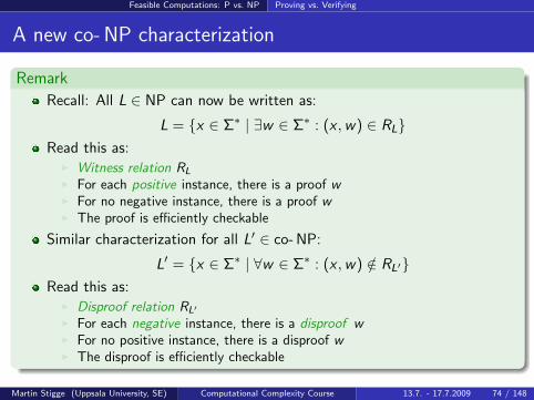
Remark
Recall: All L ∈ NP can now be written as:
L = x ∈ Σ∗ | ∃w ∈ Σ∗ : (x ,w) ∈ RLRead this as:
I Witness relation RL
I For each positive instance, there is a proof wI For no negative instance, there is a proof wI The proof is efficiently checkable
Similar characterization for all L′ ∈ co- NP:
L′ = x ∈ Σ∗ | ∀w ∈ Σ∗ : (x ,w) /∈ RL′Read this as:
I Disproof relation RL′
I For each negative instance, there is a disproof wI For no positive instance, there is a disproof wI The disproof is efficiently checkable
Martin Stigge (Uppsala University, SE) Computational Complexity Course 13.7. - 17.7.2009 74 / 148
Feasible Computations: P vs. NP Proving vs. Verifying
Boolean Formulas
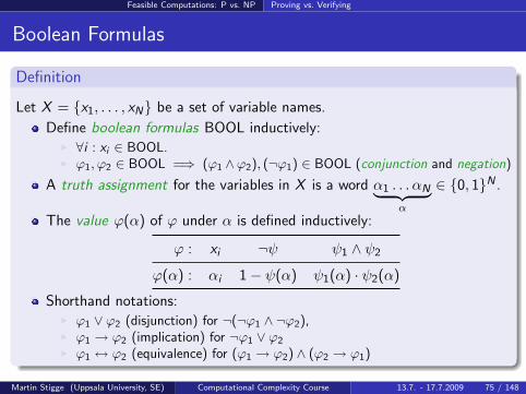
Definition
Let X = x1, . . . , xN be a set of variable names.
Define boolean formulas BOOL inductively:I ∀i : xi ∈ BOOL.I ϕ1, ϕ2 ∈ BOOL =⇒ (ϕ1 ∧ϕ2), (¬ϕ1) ∈ BOOL (conjunction and negation)
A truth assignment for the variables in X is a word α1 . . . αN︸ ︷︷ ︸α
∈ 0, 1N .
The value ϕ(α) of ϕ under α is defined inductively:
ϕ : xi ¬ψ ψ1 ∧ ψ2
ϕ(α) : αi 1− ψ(α) ψ1(α) · ψ2(α)
Shorthand notations:I ϕ1 ∨ ϕ2 (disjunction) for ¬(¬ϕ1 ∧ ¬ϕ2),I ϕ1 → ϕ2 (implication) for ¬ϕ1 ∨ ϕ2
I ϕ1 ↔ ϕ2 (equivalence) for (ϕ1 → ϕ2) ∧ (ϕ2 → ϕ1)
Martin Stigge (Uppsala University, SE) Computational Complexity Course 13.7. - 17.7.2009 75 / 148
Feasible Computations: P vs. NP Proving vs. Verifying
Example: XOR Function
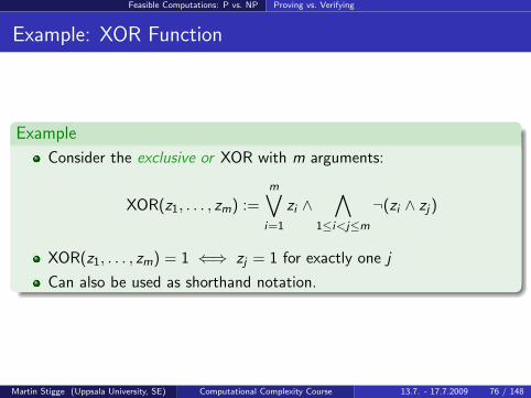
Example
Consider the exclusive or XOR with m arguments:
XOR(z1, . . . , zm) :=m∨
i=1
zi ∧∧
1≤i<j≤m
¬(zi ∧ zj)
XOR(z1, . . . , zm) = 1 ⇐⇒ zj = 1 for exactly one j
Can also be used as shorthand notation.
Martin Stigge (Uppsala University, SE) Computational Complexity Course 13.7. - 17.7.2009 76 / 148
Feasible Computations: P vs. NP Proving vs. Verifying
Example for NP: The Satisfiability Problem
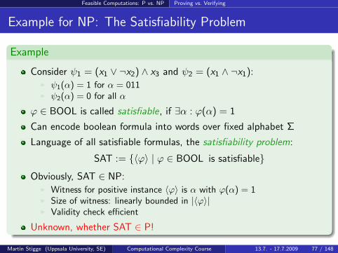
Example
Consider ψ1 = (x1 ∨ ¬x2) ∧ x3 and ψ2 = (x1 ∧ ¬x1):I ψ1(α) = 1 for α = 011I ψ2(α) = 0 for all α
ϕ ∈ BOOL is called satisfiable, if ∃α : ϕ(α) = 1
Can encode boolean formula into words over fixed alphabet Σ
Language of all satisfiable formulas, the satisfiability problem:
SAT := 〈ϕ〉 | ϕ ∈ BOOL is satisfiable
Obviously, SAT ∈ NP:I Witness for positive instance 〈ϕ〉 is α with ϕ(α) = 1I Size of witness: linearly bounded in |〈ϕ〉|I Validity check efficient
Unknown, whether SAT ∈ P!
Martin Stigge (Uppsala University, SE) Computational Complexity Course 13.7. - 17.7.2009 77 / 148
Feasible Computations: P vs. NP Reductions, Hardness, Completeness
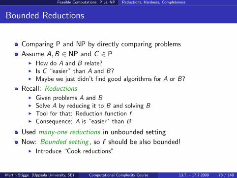
Bounded Reductions
Comparing P and NP by directly comparing problems
Assume A,B ∈ NP and C ∈ PI How do A and B relate?I Is C “easier” than A and B?I Maybe we just didn’t find good algorithms for A or B?
Recall: ReductionsI Given problems A and BI Solve A by reducing it to B and solving BI Tool for that: Reduction function fI Consequence: A is “easier” than B
Used many-one reductions in unbounded setting
Now: Bounded setting , so f should be also bounded!I Introduce “Cook reductions”
Martin Stigge (Uppsala University, SE) Computational Complexity Course 13.7. - 17.7.2009 78 / 148
Feasible Computations: P vs. NP Reductions, Hardness, Completeness
Polynomial Reduction (Cook Reduction)
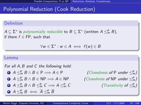
Definition
A ⊆ Σ∗ is polynomially reducible to B ⊆ Σ∗ (written A ≤pm B),
if there f ∈ FP, such that
∀w ∈ Σ∗ : w ∈ A ⇐⇒ f (w) ∈ B
Lemma
For all A,B and C the following hold:
1 A ≤pm B ∧ B ∈ P =⇒ A ∈ P (Closedness of P under ≤p
m)
2 A ≤pm B ∧ B ∈ NP =⇒ A ∈ NP (Closedness of NP under ≤p
m)
3 A ≤pm B ∧ B ≤p
m C =⇒ A ≤pm C (Transitivity of ≤p
m)
4 A ≤pm B ⇐⇒ A ≤p
m B
Martin Stigge (Uppsala University, SE) Computational Complexity Course 13.7. - 17.7.2009 79 / 148
Feasible Computations: P vs. NP Reductions, Hardness, Completeness
Hardness, Completeness
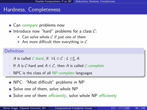
Can compare problems now
Introduce now “hard” problems for a class C:I Can solve whole C if just one of themI Are more difficult then everything in C
Definition
I A is called C-hard , if: ∀L ∈ C : L ≤pm A
I If A is C-hard and A ∈ C, then A is called C-complete
I NPC is the class of all NP-complete languages
NPC: “Most difficult” problems in NP
Solve one of them, solve whole NP
Solve one of them efficiently , solve whole NP efficiently
Martin Stigge (Uppsala University, SE) Computational Complexity Course 13.7. - 17.7.2009 80 / 148
Feasible Computations: P vs. NP Reductions, Hardness, Completeness
Hardness, Completeness: Properties
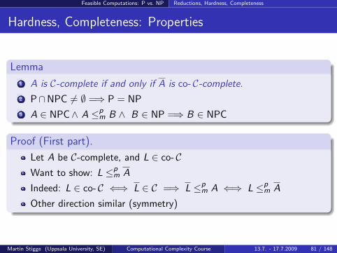
Lemma
1 A is C-complete if and only if A is co- C-complete.
2 P∩NPC 6= ∅ =⇒ P = NP
3 A ∈ NPC∧ A ≤pm B ∧ B ∈ NP =⇒ B ∈ NPC
Proof (First part).
Let A be C-complete, and L ∈ co- CWant to show: L ≤p
m A
Indeed: L ∈ co- C ⇐⇒ L ∈ C =⇒ L ≤pm A ⇐⇒ L ≤p
m A
Other direction similar (symmetry)
Martin Stigge (Uppsala University, SE) Computational Complexity Course 13.7. - 17.7.2009 81 / 148
Feasible Computations: P vs. NP Reductions, Hardness, Completeness
Hardness, Completeness: Properties (Cont.)
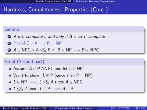
Lemma
1 A is C-complete if and only if A is co- C-complete.
2 P∩NPC 6= ∅ =⇒ P = NP
3 A ∈ NPC∧ A ≤pm B ∧ B ∈ NP =⇒ B ∈ NPC
Proof (Second part).
Assume A ∈ P∩NPC and let L ∈ NP
Want to show: L ∈ P (since then P = NP)
L ∈ NP =⇒ L ≤pm A since A ∈ NPC
L ≤pm A =⇒ L ∈ P since A ∈ P
Martin Stigge (Uppsala University, SE) Computational Complexity Course 13.7. - 17.7.2009 82 / 148
Feasible Computations: P vs. NP Reductions, Hardness, Completeness
Hardness, Completeness: Properties (Cont. 2)
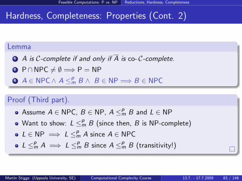
Lemma
1 A is C-complete if and only if A is co- C-complete.
2 P∩NPC 6= ∅ =⇒ P = NP
3 A ∈ NPC∧ A ≤pm B ∧ B ∈ NP =⇒ B ∈ NPC
Proof (Third part).
Assume A ∈ NPC, B ∈ NP, A ≤pm B and L ∈ NP
Want to show: L ≤pm B (since then, B is NP-complete)
L ∈ NP =⇒ L ≤pm A since A ∈ NPC
L ≤pm A =⇒ L ≤p
m B since A ≤pm B (transitivity!)
Martin Stigge (Uppsala University, SE) Computational Complexity Course 13.7. - 17.7.2009 83 / 148
Feasible Computations: P vs. NP Reductions, Hardness, Completeness
A first NP-complete Problem
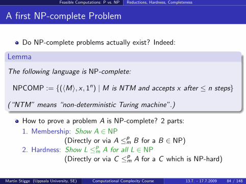
Do NP-complete problems actually exist? Indeed:
Lemma
The following language is NP-complete:
NPCOMP := (〈M〉, x , 1n) | M is NTM and accepts x after ≤ n steps
(“NTM” means “non-deterministic Turing machine”.)
How to prove a problem A is NP-complete? 2 parts:
1. Membership: Show A ∈ NP(Directly or via A ≤p
m B for a B ∈ NP)2. Hardness: Show L ≤p
m A for all L ∈ NP(Directly or via C ≤p
m A for a C which is NP-hard)
Martin Stigge (Uppsala University, SE) Computational Complexity Course 13.7. - 17.7.2009 84 / 148
Feasible Computations: P vs. NP Reductions, Hardness, Completeness
A first NP-complete Problem (Cont.)
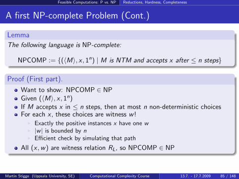
Lemma
The following language is NP-complete:
NPCOMP := (〈M〉, x , 1n) | M is NTM and accepts x after ≤ n steps
Proof (First part).
Want to show: NPCOMP ∈ NPGiven (〈M〉, x , 1n)If M accepts x in ≤ n steps, then at most n non-deterministic choicesFor each x , these choices are witness w !
I Exactly the positive instances x have one wI |w | is bounded by nI Efficient check by simulating that path
All (x ,w) are witness relation RL, so NPCOMP ∈ NP
Martin Stigge (Uppsala University, SE) Computational Complexity Course 13.7. - 17.7.2009 85 / 148
Feasible Computations: P vs. NP Reductions, Hardness, Completeness
A first NP-complete Problem (Cont. 2)
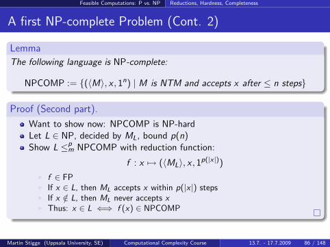
Lemma
The following language is NP-complete:
NPCOMP := (〈M〉, x , 1n) | M is NTM and accepts x after ≤ n steps
Proof (Second part).
Want to show now: NPCOMP is NP-hardLet L ∈ NP, decided by ML, bound p(n)Show L ≤p
m NPCOMP with reduction function:
f : x 7→ (〈ML〉, x , 1p(|x |))
I f ∈ FPI If x ∈ L, then ML accepts x within p(|x |) stepsI If x /∈ L, then ML never accepts xI Thus: x ∈ L ⇐⇒ f (x) ∈ NPCOMP
Martin Stigge (Uppsala University, SE) Computational Complexity Course 13.7. - 17.7.2009 86 / 148
Feasible Computations: P vs. NP NP-completeness of SAT
NP-completeness of SAT
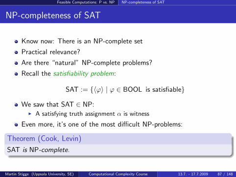
Know now: There is an NP-complete set
Practical relevance?
Are there “natural” NP-complete problems?
Recall the satisfiability problem:
SAT := 〈ϕ〉 | ϕ ∈ BOOL is satisfiable
We saw that SAT ∈ NP:I A satisfying truth assignment α is witness
Even more, it’s one of the most difficult NP-problems:
Theorem (Cook, Levin)
SAT is NP-complete.
Martin Stigge (Uppsala University, SE) Computational Complexity Course 13.7. - 17.7.2009 87 / 148
Feasible Computations: P vs. NP NP-completeness of SAT
NP-completeness of SAT: Proof ideas
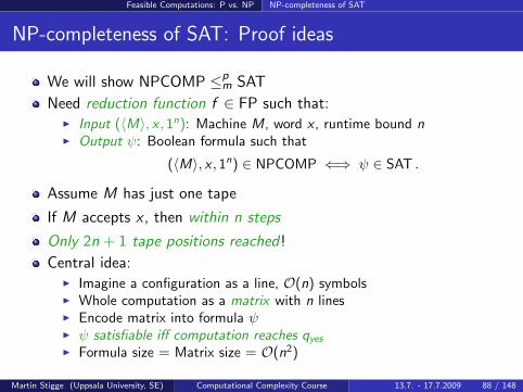
We will show NPCOMP ≤pm SAT
Need reduction function f ∈ FP such that:I Input (〈M〉, x , 1n): Machine M, word x , runtime bound nI Output ψ: Boolean formula such that
(〈M〉, x , 1n) ∈ NPCOMP ⇐⇒ ψ ∈ SAT .
Assume M has just one tape
If M accepts x , then within n steps
Only 2n + 1 tape positions reached!
Central idea:I Imagine a configuration as a line, O(n) symbolsI Whole computation as a matrix with n linesI Encode matrix into formula ψI ψ satisfiable iff computation reaches qyes
I Formula size = Matrix size = O(n2)
Martin Stigge (Uppsala University, SE) Computational Complexity Course 13.7. - 17.7.2009 88 / 148
Feasible Computations: P vs. NP NP-completeness of SAT
NP-completeness of SAT: Proof ideas (Cont.)
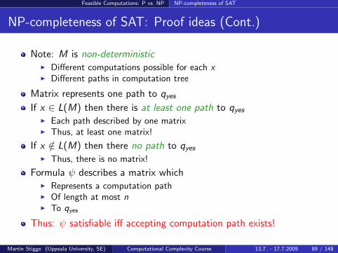
Note: M is non-deterministicI Different computations possible for each xI Different paths in computation tree
Matrix represents one path to qyes
If x ∈ L(M) then there is at least one path to qyes
I Each path described by one matrixI Thus, at least one matrix!
If x /∈ L(M) then there no path to qyes
I Thus, there is no matrix!
Formula ψ describes a matrix whichI Represents a computation pathI Of length at most nI To qyes
Thus: ψ satisfiable iff accepting computation path exists!
Martin Stigge (Uppsala University, SE) Computational Complexity Course 13.7. - 17.7.2009 89 / 148
Feasible Computations: P vs. NP NP-completeness of SAT
NP-completeness of SAT: Proof details
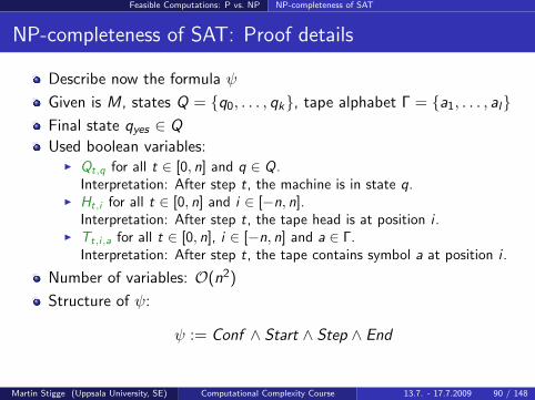
Describe now the formula ψ
Given is M, states Q = q0, . . . , qk, tape alphabet Γ = a1, . . . , alFinal state qyes ∈ Q
Used boolean variables:I Qt,q for all t ∈ [0, n] and q ∈ Q.
Interpretation: After step t, the machine is in state q.I Ht,i for all t ∈ [0, n] and i ∈ [−n, n].
Interpretation: After step t, the tape head is at position i .I Tt,i,a for all t ∈ [0, n], i ∈ [−n, n] and a ∈ Γ.
Interpretation: After step t, the tape contains symbol a at position i .
Number of variables: O(n2)
Structure of ψ:
ψ := Conf ∧ Start ∧ Step ∧ End
Martin Stigge (Uppsala University, SE) Computational Complexity Course 13.7. - 17.7.2009 90 / 148
Feasible Computations: P vs. NP NP-completeness of SAT
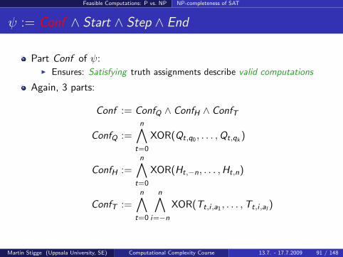
ψ := Conf ∧ Start ∧ Step ∧ End
Part Conf of ψ:I Ensures: Satisfying truth assignments describe valid computations
Again, 3 parts:
Conf := ConfQ ∧ ConfH ∧ ConfT
ConfQ :=n∧
t=0
XOR(Qt,q0 , . . . ,Qt,qk)
ConfH :=n∧
t=0
XOR(Ht,−n, . . . ,Ht,n)
ConfT :=n∧
t=0
n∧i=−n
XOR(Tt,i ,a1 , . . . ,Tt,i ,al)
Martin Stigge (Uppsala University, SE) Computational Complexity Course 13.7. - 17.7.2009 91 / 148
Feasible Computations: P vs. NP NP-completeness of SAT
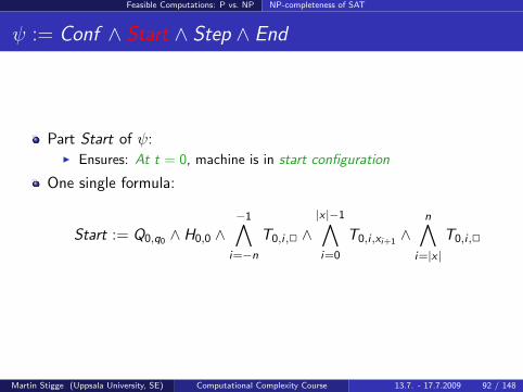
ψ := Conf ∧ Start ∧ Step ∧ End
Part Start of ψ:I Ensures: At t = 0, machine is in start configuration
One single formula:
Start := Q0,q0 ∧ H0,0 ∧−1∧
i=−n
T0,i ,2 ∧|x |−1∧i=0
T0,i ,xi+1∧
n∧i=|x |
T0,i ,2
Martin Stigge (Uppsala University, SE) Computational Complexity Course 13.7. - 17.7.2009 92 / 148
Feasible Computations: P vs. NP NP-completeness of SAT
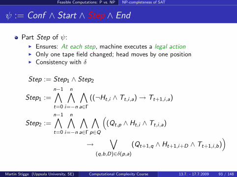
ψ := Conf ∧ Start ∧ Step ∧ End
Part Step of ψ:I Ensures: At each step, machine executes a legal actionI Only one tape field changed; head moves by one positionI Consistency with δ
Step := Step1 ∧ Step2
Step1 :=n−1∧t=0
n∧i=−n
∧a∈Γ
((¬Ht,i ∧ Tt,i ,a)→ Tt+1,i ,a)
Step2 :=n−1∧t=0
n∧i=−n
∧a∈Γ
∧p∈Q
((Qt,p ∧ Ht,i ∧ Tt,i ,a)
→∨
(q,b,D)∈δ(p,a)
(Qt+1,q ∧ Ht+1,i+D ∧ Tt+1,i ,b))
Martin Stigge (Uppsala University, SE) Computational Complexity Course 13.7. - 17.7.2009 93 / 148
Feasible Computations: P vs. NP NP-completeness of SAT
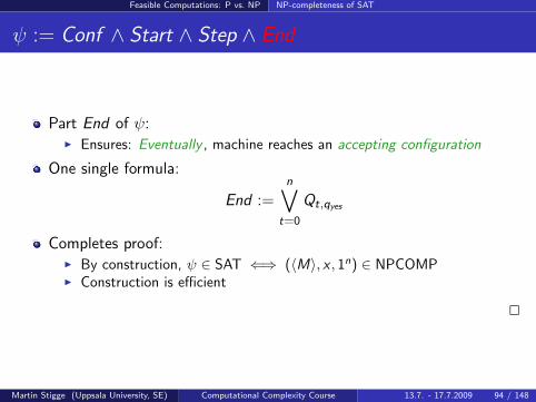
ψ := Conf ∧ Start ∧ Step ∧ End
Part End of ψ:I Ensures: Eventually , machine reaches an accepting configuration
One single formula:
End :=n∨
t=0
Qt,qyes
Completes proof:I By construction, ψ ∈ SAT ⇐⇒ (〈M〉, x , 1n) ∈ NPCOMPI Construction is efficient
2
Martin Stigge (Uppsala University, SE) Computational Complexity Course 13.7. - 17.7.2009 94 / 148
Feasible Computations: P vs. NP NP-completeness of SAT
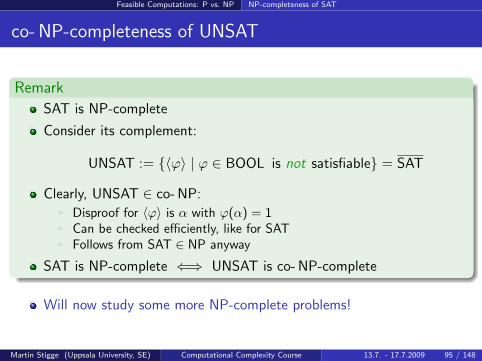
co- NP-completeness of UNSAT
Remark
SAT is NP-complete
Consider its complement:
UNSAT := 〈ϕ〉 | ϕ ∈ BOOL is not satisfiable = SAT
Clearly, UNSAT ∈ co- NP:I Disproof for 〈ϕ〉 is α with ϕ(α) = 1I Can be checked efficiently, like for SATI Follows from SAT ∈ NP anyway
SAT is NP-complete ⇐⇒ UNSAT is co- NP-complete
Will now study some more NP-complete problems!
Martin Stigge (Uppsala University, SE) Computational Complexity Course 13.7. - 17.7.2009 95 / 148
Feasible Computations: P vs. NP Natural NP-complete problems
CIRSAT: Satisfiability of Boolean Circuits
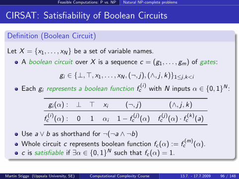
Definition (Boolean Circuit)
Let X = x1, . . . , xN be a set of variable names.
A boolean circuit over X is a sequence c = (g1, . . . , gm) of gates:
gi ∈ ⊥,>, x1, . . . , xN , (¬, j), (∧, j , k)1≤j ,k<i
Each gi represents a boolean function f(i)c with N inputs α ∈ 0, 1N :
gi (α) : ⊥ > xi (¬, j) (∧, j , k)
f(i)c (α) : 0 1 αi 1− f
(j)c (α) f
(j)c (α) · f (k)
c (a)
Use a ∨ b as shorthand for ¬(¬a ∧ ¬b)
Whole circuit c represents boolean function fc(α) := f(m)c (α).
c is satisfiable if ∃α ∈ 0, 1N such that fc(α) = 1.
Martin Stigge (Uppsala University, SE) Computational Complexity Course 13.7. - 17.7.2009 96 / 148
Feasible Computations: P vs. NP Natural NP-complete problems
CIRSAT: Satisfiability of Boolean Circuits (Cont.)
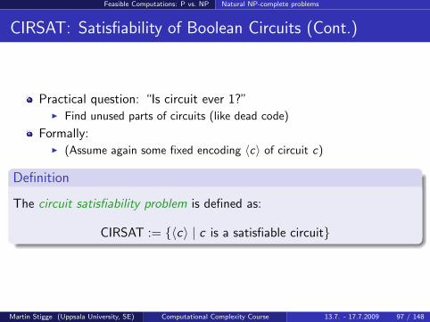
Practical question: “Is circuit ever 1?”I Find unused parts of circuits (like dead code)
Formally:I (Assume again some fixed encoding 〈c〉 of circuit c)
Definition
The circuit satisfiability problem is defined as:
CIRSAT := 〈c〉 | c is a satisfiable circuit
Martin Stigge (Uppsala University, SE) Computational Complexity Course 13.7. - 17.7.2009 97 / 148
Feasible Computations: P vs. NP Natural NP-complete problems
CIRSAT: Satisfiability of Boolean Circuits (Cont. 2)
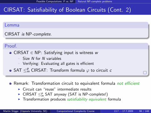
Lemma
CIRSAT is NP-complete.
Proof.
CIRSAT ∈ NP: Satisfying input is witness wI Size N for N variablesI Verifying: Evaluating all gates is efficient
SAT ≤pm CIRSAT: Transform formula ϕ to circuit c
Remark: Transformation circuit to equivalent formula not efficientI Circuit can “reuse” intermediate resultsI CIRSAT ≤p
m SAT anyway (SAT is NP-complete!)I Transformation produces satisfiability equivalent formula
Martin Stigge (Uppsala University, SE) Computational Complexity Course 13.7. - 17.7.2009 98 / 148
Feasible Computations: P vs. NP Natural NP-complete problems
CNF: Restricted Structure of Boolean Formulas
Definition (CNF)
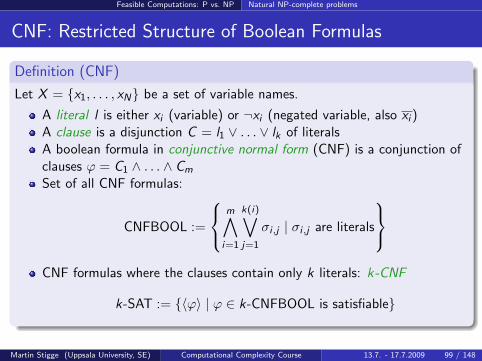
Let X = x1, . . . , xN be a set of variable names.
A literal l is either xi (variable) or ¬xi (negated variable, also xi )A clause is a disjunction C = l1 ∨ . . . ∨ lk of literalsA boolean formula in conjunctive normal form (CNF) is a conjunction ofclauses ϕ = C1 ∧ . . . ∧ Cm
Set of all CNF formulas:
CNFBOOL :=
m∧
i=1
k(i)∨j=1
σi ,j | σi ,j are literals
CNF formulas where the clauses contain only k literals: k-CNF
k-SAT := 〈ϕ〉 | ϕ ∈ k-CNFBOOL is satisfiable
Martin Stigge (Uppsala University, SE) Computational Complexity Course 13.7. - 17.7.2009 99 / 148
Feasible Computations: P vs. NP Natural NP-complete problems
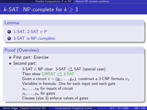
k-SAT: NP-complete for k ≥ 3
Lemma
1 1-SAT, 2-SAT ∈ P
2 3-SAT is NP-complete.
Proof (Overview).
First part: Exercise
Second part:I 3-SAT ∈ NP clear: 3-SAT ≤p
m SAT (special case)I Then show CIRSAT ≤p
m 3-SATI Given a circuit c = (g1, . . . , gm), construct a 3-CNF formula ψc
I Variables in formula: One for each input and each gateI x1, . . . , xN for inputs of circuitI y1, . . . , ym for gatesI Clauses (size 3) enforce values of gates
Martin Stigge (Uppsala University, SE) Computational Complexity Course 13.7. - 17.7.2009 100 / 148
Feasible Computations: P vs. NP Natural NP-complete problems
NP-completeness of 3-SAT
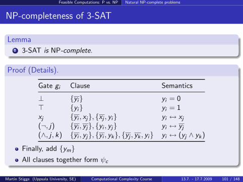
Lemma2 3-SAT is NP-complete.
Proof (Details).
Gate gi Clause Semantics
⊥ yi yi = 0> yi yi = 1xj yi , xj, xj , yi yi ↔ xj
(¬, j) yi , yj, yi , yj yi ↔ yj
(∧, j , k) yi , yj, yi , yk, yj , yk , yi yi ↔ (yj ∧ yk)
Finally, add ymAll clauses together form ψc
Martin Stigge (Uppsala University, SE) Computational Complexity Course 13.7. - 17.7.2009 101 / 148
Feasible Computations: P vs. NP Natural NP-complete problems
NP-completeness of 3-SAT (Cont.)
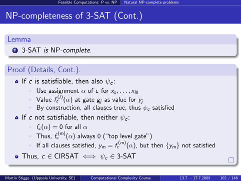
Lemma2 3-SAT is NP-complete.
Proof (Details, Cont.).
If c is satisfiable, then also ψc :I Use assignment α of c for x1, . . . , xN
I Value f(j)c (α) at gate gj as value for yj
I By construction, all clauses true, thus ψc satisfied
If c not satisfiable, then neither ψc :I fc(α) = 0 for all αI Thus, f
(m)c (α) always 0 (“top level gate”)
I If all clauses satisfied, ym = f(m)c (α), but then ym not satisfied
Thus, c ∈ CIRSAT ⇐⇒ ψc ∈ 3-SAT
Martin Stigge (Uppsala University, SE) Computational Complexity Course 13.7. - 17.7.2009 102 / 148
Feasible Computations: P vs. NP Natural NP-complete problems
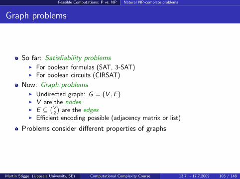
Graph problems
So far: Satisfiability problemsI For boolean formulas (SAT, 3-SAT)I For boolean circuits (CIRSAT)
Now: Graph problemsI Undirected graph: G = (V ,E )I V are the nodesI E ⊆
(V2
)are the edges
I Efficient encoding possible (adjacency matrix or list)
Problems consider different properties of graphs
Martin Stigge (Uppsala University, SE) Computational Complexity Course 13.7. - 17.7.2009 103 / 148
Feasible Computations: P vs. NP Natural NP-complete problems
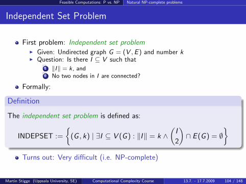
Independent Set Problem
First problem: Independent set problemI Given: Undirected graph G = (V ,E ) and number kI Question: Is there I ⊆ V such that
1 ‖I‖ = k, and2 No two nodes in I are connected?
Formally:
Definition
The independent set problem is defined as:
INDEPSET :=
(G , k) | ∃I ⊆ V (G ) : ‖I‖ = k ∧
(I
2
)∩ E (G ) = ∅
Turns out: Very difficult (i.e. NP-complete)
Martin Stigge (Uppsala University, SE) Computational Complexity Course 13.7. - 17.7.2009 104 / 148
Feasible Computations: P vs. NP Natural NP-complete problems
INDEPSET is NP-complete
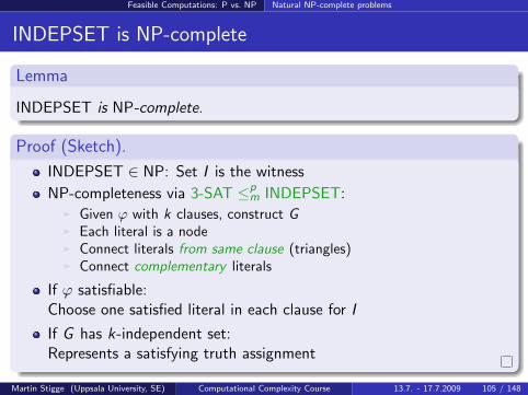
Lemma
INDEPSET is NP-complete.
Proof (Sketch).
INDEPSET ∈ NP: Set I is the witness
NP-completeness via 3-SAT ≤pm INDEPSET:
I Given ϕ with k clauses, construct GI Each literal is a nodeI Connect literals from same clause (triangles)I Connect complementary literals
If ϕ satisfiable:Choose one satisfied literal in each clause for I
If G has k-independent set:Represents a satisfying truth assignment
Martin Stigge (Uppsala University, SE) Computational Complexity Course 13.7. - 17.7.2009 105 / 148
Feasible Computations: P vs. NP Natural NP-complete problems
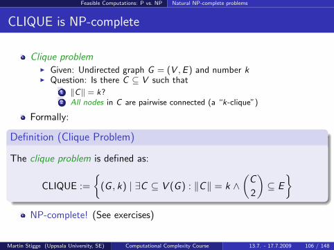
CLIQUE is NP-complete
Clique problemI Given: Undirected graph G = (V ,E ) and number kI Question: Is there C ⊆ V such that
1 ‖C‖ = k?2 All nodes in C are pairwise connected (a “k-clique”)
Formally:
Definition (Clique Problem)
The clique problem is defined as:
CLIQUE :=
(G , k) | ∃C ⊆ V (G ) : ‖C‖ = k ∧
(C
2
)⊆ E
NP-complete! (See exercises)
Martin Stigge (Uppsala University, SE) Computational Complexity Course 13.7. - 17.7.2009 106 / 148
Feasible Computations: P vs. NP Natural NP-complete problems
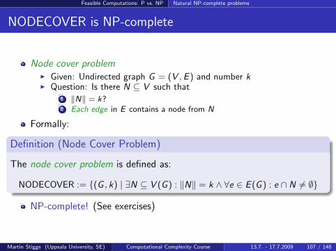
NODECOVER is NP-complete
Node cover problemI Given: Undirected graph G = (V ,E ) and number kI Question: Is there N ⊆ V such that
1 ‖N‖ = k?2 Each edge in E contains a node from N
Formally:
Definition (Node Cover Problem)
The node cover problem is defined as:
NODECOVER := (G , k) | ∃N ⊆ V (G ) : ‖N‖ = k ∧ ∀e ∈ E (G ) : e ∩ N 6= ∅
NP-complete! (See exercises)
Martin Stigge (Uppsala University, SE) Computational Complexity Course 13.7. - 17.7.2009 107 / 148
Feasible Computations: P vs. NP Natural NP-complete problems
HAMILTONPATH is NP-complete
Hamilton path problemI Given: Undirected graph G = (V ,E )I Question: Is there a path p = (p0, . . . , pk) in G such that:
F All nodes pi are pairwise different? (“Hamilton path”)
Formally:
Definition (Hamilton Path Problem)
The Hamilton Path Problem is defined as:
HAMILTONPATH := G | ∃p : p is Hamilton path in G
NP-complete!
Martin Stigge (Uppsala University, SE) Computational Complexity Course 13.7. - 17.7.2009 108 / 148
Feasible Computations: P vs. NP Natural NP-complete problems
HITTINGSET is NP-complete
Hitting set problemI Given:
F A set AF A collection C = (C1, . . . Cm) of subsets of A: ∀i : Ci ⊆ AF A number k
I Question: Is there a set H ⊆ A such that:1 ‖H‖ = k2 H contains an element from each Ci ∈ C (“k-hitting set”)
Not a graph problem, but related
Formally:
Definition (Hitting Set Problem)
The hitting set problem is defined as:
HITTINGSET := (A,C , k) | ∃H ⊆ A : ‖H‖ = k ∧ ∀Ci ∈ C : H ∩ Ci 6= ∅
NP-complete! (See exercises)
Martin Stigge (Uppsala University, SE) Computational Complexity Course 13.7. - 17.7.2009 109 / 148
Feasible Computations: P vs. NP Natural NP-complete problems
TSP is NP-complete
Travelling Salesman ProblemI Given:
F n cities with a distance matrix D ∈ Nn×n
F A number kI Question: Is there a tour through all cities such that
1 Each city is visited exactly once, and2 The distance sum of the tour is at most k?
Formally:
Definition (Travelling Salesman Problem)
The Travelling salesman problem is defined as:
TSP :=
(D, k) | ∃π :
n∑i=1
D[π(i), π(i + 1)] ≤ k
NP-complete!
Martin Stigge (Uppsala University, SE) Computational Complexity Course 13.7. - 17.7.2009 110 / 148
Feasible Computations: P vs. NP Natural NP-complete problems
KNAPSACK is NP-complete
Knapsack ProblemI Given:
F n items with values V = (v1, . . . , vn) and weights W = (w1, . . . , wn)F A lower value limit l and an upper weight limit m
I Question: Is there a selection S ⊆ [1, n] of the items, such that1 The sum of the values is at least l , and2 The sum of the weights is at most m?
Formally:
Definition (Knapsack problem)
The Knapsack problem is defined as:
KNAPSACK :=
(V ,W , l ,m) | ∃S ⊆ [1, n] :
∑i∈S
wi ≤ l ∧∑i∈S
vi ≥ m
NP-complete!
Martin Stigge (Uppsala University, SE) Computational Complexity Course 13.7. - 17.7.2009 111 / 148
Feasible Computations: P vs. NP Natural NP-complete problems
ILP is NP-complete
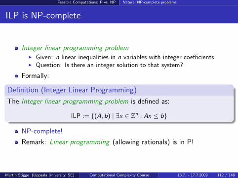
Integer linear programming problemI Given: n linear inequalities in n variables with integer coefficientsI Question: Is there an integer solution to that system?
Formally:
Definition (Integer Linear Programming)
The Integer linear programming problem is defined as:
ILP := (A, b) | ∃x ∈ Zn : Ax ≤ b
NP-complete!
Remark: Linear programming (allowing rationals) is in P!
Martin Stigge (Uppsala University, SE) Computational Complexity Course 13.7. - 17.7.2009 112 / 148
Feasible Computations: P vs. NP Natural NP-complete problems
BINPACK is NP-complete
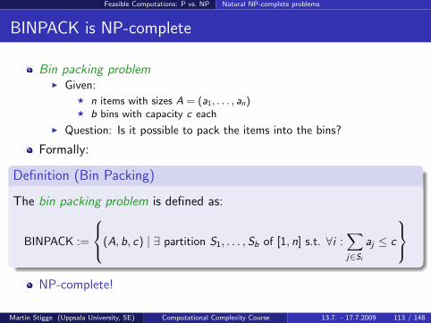
Bin packing problemI Given:
F n items with sizes A = (a1, . . . , an)F b bins with capacity c each
I Question: Is it possible to pack the items into the bins?
Formally:
Definition (Bin Packing)
The bin packing problem is defined as:
BINPACK :=
(A, b, c) | ∃ partition S1, . . . ,Sb of [1, n] s.t. ∀i :∑j∈Si
aj ≤ c
NP-complete!
Martin Stigge (Uppsala University, SE) Computational Complexity Course 13.7. - 17.7.2009 113 / 148
Feasible Computations: P vs. NP Beyond NP-completeness
Between P and NPC
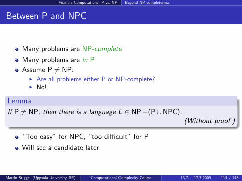
Many problems are NP-complete
Many problems are in P
Assume P 6= NP:I Are all problems either P or NP-complete?I No!
Lemma
If P 6= NP, then there is a language L ∈ NP−(P∪NPC).(Without proof.)
“Too easy” for NPC, “too difficult” for P
Will see a candidate later
Martin Stigge (Uppsala University, SE) Computational Complexity Course 13.7. - 17.7.2009 114 / 148
Feasible Computations: P vs. NP Beyond NP-completeness
Pseudo-polynomial complexity
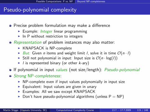
Precise problem formulation may make a differenceI Example: Integer linear programmingI In P without restriction to integers
Representation of problem instances may also matter:I KNAPSACK is NP-completeI But: Given n items and weight limit l , solve it in time O(n · l)I Still not polynomial in input: Input size is O(n · log(l))I l is represented binary (or other k-ary)
If polynomial in input values (not size/length): Pseudo-polynomial
Strong NP-completeness:I NP-complete even if input values polynomially in input sizeI Equivalent: Input values are given in unaryI Examples: All we saw except KNAPSACKI Don’t have pseudo-polynomial algorithms (unless P = NP)
Martin Stigge (Uppsala University, SE) Computational Complexity Course 13.7. - 17.7.2009 115 / 148
Feasible Computations: P vs. NP Beyond NP-completeness
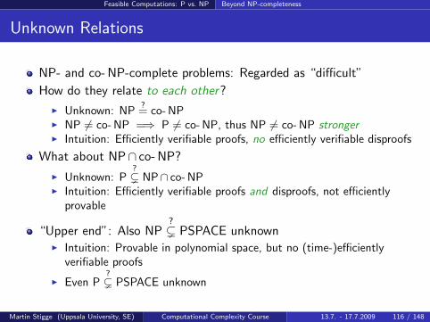
Unknown Relations
NP- and co- NP-complete problems: Regarded as “difficult”
How do they relate to each other?
I Unknown: NP?= co- NP
I NP 6= co- NP =⇒ P 6= co- NP, thus NP 6= co- NP strongerI Intuition: Efficiently verifiable proofs, no efficiently verifiable disproofs
What about NP∩ co- NP?
I Unknown: P?( NP∩ co- NP
I Intuition: Efficiently verifiable proofs and disproofs, not efficientlyprovable
“Upper end”: Also NP?( PSPACE unknown
I Intuition: Provable in polynomial space, but no (time-)efficientlyverifiable proofs
I Even P?( PSPACE unknown
Martin Stigge (Uppsala University, SE) Computational Complexity Course 13.7. - 17.7.2009 116 / 148
Feasible Computations: P vs. NP Beyond NP-completeness
The Problems PRIMES and GI
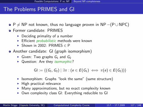
P 6= NP not known, thus no language proven in NP−(P∪NPC)
Former candidate: PRIMESI Deciding primality of a numberI Efficient probabilistic methods were knownI Shown in 2002: PRIMES ∈ P
Another candidate: GI (graph isomorphism)I Given: Two graphs G1 and G2
I Question: Are they isomorphic?
GI := (G1,G2) | ∃π : (e ∈ E (G1) ⇐⇒ π(e) ∈ E (G2))
I Isomorphism: Graphs “look the same” (same structure)I High practical relevanceI Many approximations, but no exact complexity knownI Own complexity class GI: Everything reducible to GI
Martin Stigge (Uppsala University, SE) Computational Complexity Course 13.7. - 17.7.2009 117 / 148
Advanced Complexity Concepts
Course Outline
0 Introduction
1 Basic Computability TheoryFormal LanguagesModel of Computation: Turing MachinesDecidability, Undecidability, Semi-Decidability
2 Complexity ClassesLandau Symbols: The O(·) NotationTime and Space ComplexityRelations between Complexity Classes
3 Feasible Computations: P vs. NPProving vs. VerifyingReductions, Hardness, CompletenessNatural NP-complete problems
4 Advanced Complexity ConceptsNon-uniform ComplexityProbabilistic Complexity ClassesInteractive Proof Systems
Martin Stigge (Uppsala University, SE) Computational Complexity Course 13.7. - 17.7.2009 118 / 148
Advanced Complexity Concepts
Course Outline
0 Introduction
1 Basic Computability TheoryFormal LanguagesModel of Computation: Turing MachinesDecidability, Undecidability, Semi-Decidability
2 Complexity ClassesLandau Symbols: The O(·) NotationTime and Space ComplexityRelations between Complexity Classes
3 Feasible Computations: P vs. NPProving vs. VerifyingReductions, Hardness, CompletenessNatural NP-complete problems
4 Advanced Complexity ConceptsNon-uniform ComplexityProbabilistic Complexity ClassesInteractive Proof Systems
Martin Stigge (Uppsala University, SE) Computational Complexity Course 13.7. - 17.7.2009 119 / 148
Advanced Complexity Concepts Non-uniform Complexity
Uniform vs. Non-uniform Models
Turing Machine: One fixed (finite) machine for all input sizes
“One size fits it all” approach, uniform model
Some situations: More hardwired information when size growsI Cryptography: Precomputed tables for different key sizesI Want to model such attackers
Model this non-uniform notion using advice:I Machine gets advice string an in addition to inputI One fixed string an for each input size n
Martin Stigge (Uppsala University, SE) Computational Complexity Course 13.7. - 17.7.2009 120 / 148
Advanced Complexity Concepts Non-uniform Complexity
Turing Machine with Advice
Definition (Turing Machine with Advice)
A Turing machine with advice is a 6-tuple M = (Q, Γ, δ, q0,F ,A)with Q, Γ, δ, q0,F as before and A = ann≥0
The set a A is called the advice.
Language accepted by M:
L(M) := x ∈ Σ∗ | ∃y , z ∈ Γ∗ : (ε, q0, x#a|x |) `∗ (y , qyes , z)
(Separation symbol # ∈ Γ)
Martin Stigge (Uppsala University, SE) Computational Complexity Course 13.7. - 17.7.2009 121 / 148
Advanced Complexity Concepts Non-uniform Complexity
Turing Machine with Advice: Remarks
Classical Turing machine: Finite object
Advice: Infinite object, external information to machine
Difference to witness from NP:I Witness was different for each input, a specific proofI Only for the positive instances x ∈ L(M)I Advice is for each input size, a static computational “aid”I Fixed, the same an for each x of length n
Very powerful without restrictions:I Any language L (even undecidable!) could be decidedI Encode into an a large table with all words Σn
I For each word x a bit: x ∈ L or x /∈ LI Machine can look up in table
Martin Stigge (Uppsala University, SE) Computational Complexity Course 13.7. - 17.7.2009 122 / 148
Advanced Complexity Concepts Non-uniform Complexity
Restricting the Advice: P/poly
Restrict now advice polynomially
Definition
P/poly is the set of all languages L such that:
1 L is decided by a TM M with advice A exists, and
2 ∀n : |an| ≤ p(n) for some polynomial p(n).
Clear: P ⊆ P/poly (just ignore the advice)
Thus: If ∃L ∈ NP with L /∈ P/poly then P 6= NP!
Difficulty: P/poly is powerful, contains still undecidable languages
Martin Stigge (Uppsala University, SE) Computational Complexity Course 13.7. - 17.7.2009 123 / 148
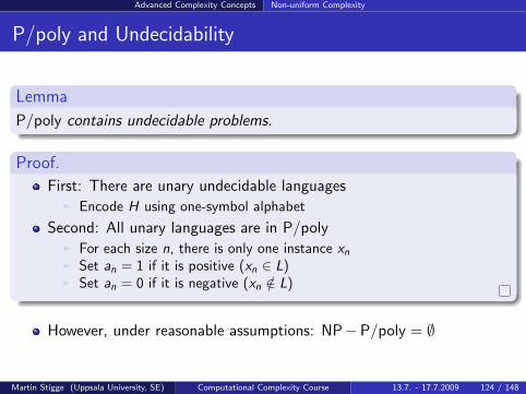
Advanced Complexity Concepts Non-uniform Complexity
P/poly and Undecidability
Lemma
P/poly contains undecidable problems.
Proof.
First: There are unary undecidable languagesI Encode H using one-symbol alphabet
Second: All unary languages are in P/polyI For each size n, there is only one instance xn
I Set an = 1 if it is positive (xn ∈ L)I Set an = 0 if it is negative (xn /∈ L)
However, under reasonable assumptions: NP−P/poly = ∅
Martin Stigge (Uppsala University, SE) Computational Complexity Course 13.7. - 17.7.2009 124 / 148
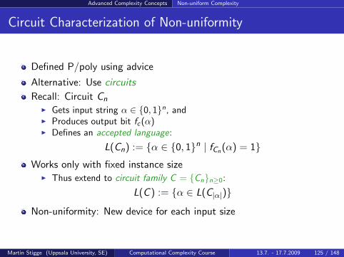
Advanced Complexity Concepts Non-uniform Complexity
Circuit Characterization of Non-uniformity
Defined P/poly using advice
Alternative: Use circuits
Recall: Circuit Cn
I Gets input string α ∈ 0, 1n, andI Produces output bit fc(α)I Defines an accepted language:
L(Cn) := α ∈ 0, 1n | fCn(α) = 1Works only with fixed instance size
I Thus extend to circuit family C = Cnn≥0:
L(C ) := α ∈ L(C|α|)
Non-uniformity: New device for each input size
Martin Stigge (Uppsala University, SE) Computational Complexity Course 13.7. - 17.7.2009 125 / 148
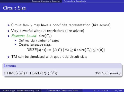
Advanced Complexity Concepts Non-uniform Complexity
Circuit Size
Circuit family may have a non-finite representation (like advice)
Very powerful without restrictions (like advice)
Resource bound : size(Cn)I Defined via number of gatesI Creates language class:
DSIZE(s(n)) := L(C ) | ∀n ≥ 0 : size(Cn) ≤ s(n)
TM can be simulated with quadratic circuit size:
Lemma
DTIME(t(n)) ⊆ DSIZE(O(t(n)2)) (Without proof.)
Martin Stigge (Uppsala University, SE) Computational Complexity Course 13.7. - 17.7.2009 126 / 148
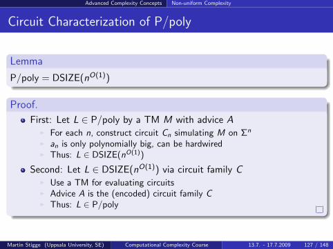
Advanced Complexity Concepts Non-uniform Complexity
Circuit Characterization of P/poly
Lemma
P/poly = DSIZE(nO(1))
Proof.
First: Let L ∈ P/poly by a TM M with advice AI For each n, construct circuit Cn simulating M on Σn
I an is only polynomially big, can be hardwiredI Thus: L ∈ DSIZE(nO(1))
Second: Let L ∈ DSIZE(nO(1)) via circuit family CI Use a TM for evaluating circuitsI Advice A is the (encoded) circuit family CI Thus: L ∈ P/poly
Martin Stigge (Uppsala University, SE) Computational Complexity Course 13.7. - 17.7.2009 127 / 148
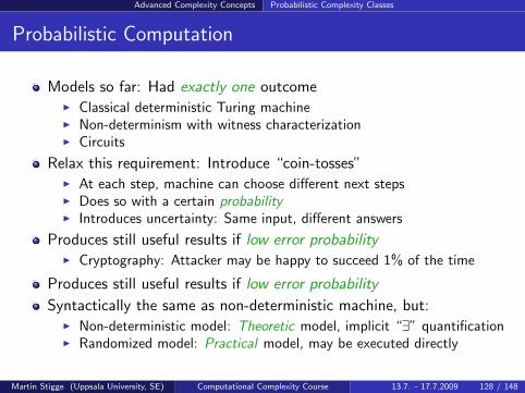
Advanced Complexity Concepts Probabilistic Complexity Classes
Probabilistic Computation
Models so far: Had exactly one outcomeI Classical deterministic Turing machineI Non-determinism with witness characterizationI Circuits
Relax this requirement: Introduce “coin-tosses”I At each step, machine can choose different next stepsI Does so with a certain probabilityI Introduces uncertainty: Same input, different answers
Produces still useful results if low error probabilityI Cryptography: Attacker may be happy to succeed 1% of the time
Produces still useful results if low error probability
Syntactically the same as non-deterministic machine, but:I Non-deterministic model: Theoretic model, implicit “∃” quantificationI Randomized model: Practical model, may be executed directly
Martin Stigge (Uppsala University, SE) Computational Complexity Course 13.7. - 17.7.2009 128 / 148
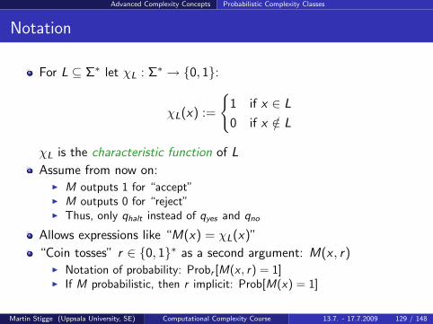
Advanced Complexity Concepts Probabilistic Complexity Classes
Notation
For L ⊆ Σ∗ let χL : Σ∗ → 0, 1:
χL(x) :=
1 if x ∈ L
0 if x /∈ L
χL is the characteristic function of L
Assume from now on:I M outputs 1 for “accept”I M outputs 0 for “reject”I Thus, only qhalt instead of qyes and qno
Allows expressions like “M(x) = χL(x)”
“Coin tosses” r ∈ 0, 1∗ as a second argument: M(x , r)I Notation of probability: Probr [M(x , r) = 1]I If M probabilistic, then r implicit: Prob[M(x) = 1]
Martin Stigge (Uppsala University, SE) Computational Complexity Course 13.7. - 17.7.2009 129 / 148
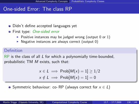
Advanced Complexity Concepts Probabilistic Complexity Classes
One-sided Error: The class RP
Didn’t define accepted languages yet
First type: One-sided errorI Positive instances may be judged wrong (output 0 or 1)I Negative instances are always correct (output 0)
Definition
RP is the class of all L for which a polynomially time-bounded,probabilistic TM M exists, such that:
x ∈ L =⇒ Prob[M(x) = 1] ≥ 1/2
x /∈ L =⇒ Prob[M(x) = 1] = 0
Symmetric behaviour: co- RP (always correct for x ∈ L)
Martin Stigge (Uppsala University, SE) Computational Complexity Course 13.7. - 17.7.2009 130 / 148
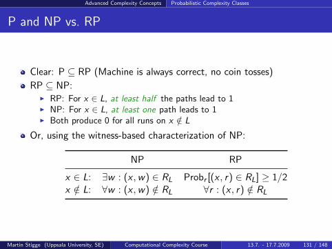
Advanced Complexity Concepts Probabilistic Complexity Classes
P and NP vs. RP
Clear: P ⊆ RP (Machine is always correct, no coin tosses)
RP ⊆ NP:I RP: For x ∈ L, at least half the paths lead to 1I NP: For x ∈ L, at least one path leads to 1I Both produce 0 for all runs on x /∈ L
Or, using the witness-based characterization of NP:
NP RP
x ∈ L: ∃w : (x ,w) ∈ RL Probr [(x , r) ∈ RL] ≥ 1/2x /∈ L: ∀w : (x ,w) /∈ RL ∀r : (x , r) /∈ RL
Martin Stigge (Uppsala University, SE) Computational Complexity Course 13.7. - 17.7.2009 131 / 148
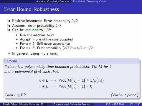
Advanced Complexity Concepts Probabilistic Complexity Classes
Error Bound Robustness
Positive instances: Error probability 1/2Assume: Error probability 2/3Can be reduced to 1/2:
I Run the machine twiceI Accept, if one of the runs acceptedI For x /∈ L: Still never acceptanceI For x ∈ L: Error probability (2/3)2 = 4/9 < 1/2
In general, using more runs:
Lemma
If there is a polynomially time-bounded probabilistic TM M for Land a polynomial p(n) such that:
x ∈ L =⇒ Prob[M(x) = 1] ≥ 1/p(|x |)x /∈ L =⇒ Prob[M(x) = 1] = 0
Then L ∈ RP. (Without proof.)
Martin Stigge (Uppsala University, SE) Computational Complexity Course 13.7. - 17.7.2009 132 / 148
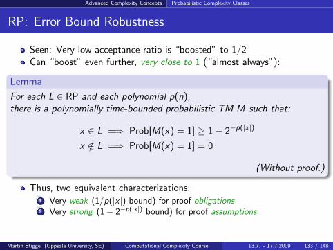
Advanced Complexity Concepts Probabilistic Complexity Classes
RP: Error Bound Robustness
Seen: Very low acceptance ratio is “boosted” to 1/2Can “boost” even further, very close to 1 (“almost always”):
Lemma
For each L ∈ RP and each polynomial p(n),there is a polynomially time-bounded probabilistic TM M such that:
x ∈ L =⇒ Prob[M(x) = 1] ≥ 1− 2−p(|x |)
x /∈ L =⇒ Prob[M(x) = 1] = 0
(Without proof.)
Thus, two equivalent characterizations:1 Very weak (1/p(|x |) bound) for proof obligations2 Very strong (1− 2−p(|x|) bound) for proof assumptions
Martin Stigge (Uppsala University, SE) Computational Complexity Course 13.7. - 17.7.2009 133 / 148
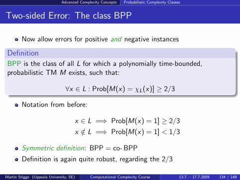
Advanced Complexity Concepts Probabilistic Complexity Classes
Two-sided Error: The class BPP
Now allow errors for positive and negative instances
Definition
BPP is the class of all L for which a polynomially time-bounded,probabilistic TM M exists, such that:
∀x ∈ L : Prob[M(x) = χL(x)] ≥ 2/3
Notation from before:
x ∈ L =⇒ Prob[M(x) = 1] ≥ 2/3
x /∈ L =⇒ Prob[M(x) = 1] < 1/3
Symmetric definition: BPP = co- BPP
Definition is again quite robust, regarding the 2/3
Martin Stigge (Uppsala University, SE) Computational Complexity Course 13.7. - 17.7.2009 134 / 148
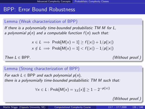
Advanced Complexity Concepts Probabilistic Complexity Classes
BPP: Error Bound Robustness
Lemma (Weak characterization of BPP)
If there is a polynomially time-bounded probabilistic TM M for L,a polynomial p(n) and a computable function f (n) such that:
x ∈ L =⇒ Prob[M(x) = 1] ≥ f (|x |) + 1/p(|x |)x /∈ L =⇒ Prob[M(x) = 1] < f (|x |)− 1/p(|x |)
Then L ∈ BPP. (Without proof.)
Lemma (Strong characterization of BPP)
For each L ∈ BPP and each polynomial p(n),there is a polynomially time-bounded probabilistic TM M such that:
∀x ∈ L : Prob[M(x) = χL(x)] ≥ 1− 2−p(|x |)
(Without proof.)
Martin Stigge (Uppsala University, SE) Computational Complexity Course 13.7. - 17.7.2009 135 / 148
Advanced Complexity Concepts Probabilistic Complexity Classes
Relations of BPP
Clearly RP ⊆ BPP (no error for x /∈ L with RP)
Unknown relation between BPP and NP
Note: Error rate can be made exponentially small
“Efficient computation” nowadays often characterized with BPPI In fact, P = BPP is a popular conjecture
Martin Stigge (Uppsala University, SE) Computational Complexity Course 13.7. - 17.7.2009 136 / 148
Advanced Complexity Concepts Probabilistic Complexity Classes
Monte Carlo vs. Las Vegas
Described machines always answer, sometimes wrongI Monte Carlo Algorithms
Contrast: Always answer right, but sometimes with “I don’t know”I Las Vegas Algorithms
Denote “I don’t know” with “⊥”
Definition
ZPP is the class of all L for which a polynomially time-bounded,probabilistic TM M exists, such that:
I ∀x ∈ L : Prob[M(x) = ⊥] ≤ 1/2, and
I ∀x ∈ L, r : M(x , r) 6= ⊥ =⇒ M(x , r) = χL(x)
Martin Stigge (Uppsala University, SE) Computational Complexity Course 13.7. - 17.7.2009 137 / 148
Advanced Complexity Concepts Probabilistic Complexity Classes
More Class Relationships
Lemma1 P ⊆ ZPP ⊆ RP ⊆ BPP
2 ZPP = RP∩ co- RP
3 BPP ⊆ P/poly
4 BPP = P if pseudo random number generators exist.(Efficient derandomization)
(Without proof.)
Pseudo random number generators (PRNGs) output looks randomI No observer can tell the differenceI No observer can predict the next bitI PRNGs exist under certain (sophisticated) assumptions
Martin Stigge (Uppsala University, SE) Computational Complexity Course 13.7. - 17.7.2009 138 / 148
Advanced Complexity Concepts Interactive Proof Systems
Intuitive Notion of a Proof
Proof: Prover and Verifier
Prover convinces verifier of validity of some assertion
In mathematics:I Prover writes down a list of stepsI Verifier checks each step
In general:I Interaction between the partiesI Verifier asks questions (possibly adaptively)I Prover answers them
Careful verifier is only convinced of valid assertions
Martin Stigge (Uppsala University, SE) Computational Complexity Course 13.7. - 17.7.2009 139 / 148
Advanced Complexity Concepts Interactive Proof Systems
Formalizing the Notion of a Proof
Interpret NP as non-interactive proofs:I Supplied witness is the proofI Machine checking it is the verifier, working efficientlyI Only true assertions (“x ∈ L”) have a proofI “NP proof system”
General notion with similar properties:1 Efficiency of the verifier2 Correctness requirement:
Completeness: Each true assertion has a convincing proof strategySoundness: No false assertion has a convincing proof strategy
Will use Interactive Turing Machines for that
Martin Stigge (Uppsala University, SE) Computational Complexity Course 13.7. - 17.7.2009 140 / 148
Advanced Complexity Concepts Interactive Proof Systems
Interactive Turing Machine (ITM)
Like ordinary Turing machine, but withI Communication tape andI Two communication states q? and q!
Operation of two composed machines 〈M1,M2〉:I M1 starts in q0, M2 waits in q?
I M1 runs, writes message on shared communication tapeI M1 switches to q?, M2 switches to q!
I M2 runs, M1 waitsI .. And so on, back and forth ..I Finally, M2 stops
Period between control switches: A round
Output: Tape contents of M2 after halting
Martin Stigge (Uppsala University, SE) Computational Complexity Course 13.7. - 17.7.2009 141 / 148
Advanced Complexity Concepts Interactive Proof Systems
Interactive Proof System
Definition (Interactive Proof System)
An interactive proof system for L is a pair 〈P,V 〉 of ITMs with:
1 V is probabilistic and polynomially time-bounded.
2 Correctness requirement:
Completeness: ∀x ∈ L : Prob[〈P,V 〉(x) = 1] ≥ 2/3Soundness: ∀x /∈ L : ∀P∗ : Prob[〈P∗,V 〉(x) = 1] < 1/3
Correctness is probabilistic
Bounds:I Verifier is boundedI Prover is not bounded
Soundness is against all provers (incl. very bad ones)
Useful model for cryptographic protocols
Martin Stigge (Uppsala University, SE) Computational Complexity Course 13.7. - 17.7.2009 142 / 148
Advanced Complexity Concepts Interactive Proof Systems
IP hierarchy
Definition (IP hierarchy)
Let r : N→ N.
IP(r(n)) contains all L for with interactive proof systems 〈P,V 〉such that on common input x , at most r(|x |) rounds are used.
IP contains all L having interactive proof systems:
IP :=⋃r
IP(r(n))
Martin Stigge (Uppsala University, SE) Computational Complexity Course 13.7. - 17.7.2009 143 / 148
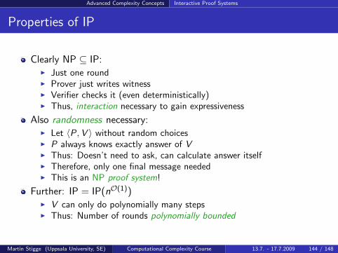
Advanced Complexity Concepts Interactive Proof Systems
Properties of IP
Clearly NP ⊆ IP:I Just one roundI Prover just writes witnessI Verifier checks it (even deterministically)I Thus, interaction necessary to gain expressiveness
Also randomness necessary:I Let 〈P,V 〉 without random choicesI P always knows exactly answer of VI Thus: Doesn’t need to ask, can calculate answer itselfI Therefore, only one final message neededI This is an NP proof system!
Further: IP = IP(nO(1))I V can only do polynomially many stepsI Thus: Number of rounds polynomially bounded
Martin Stigge (Uppsala University, SE) Computational Complexity Course 13.7. - 17.7.2009 144 / 148
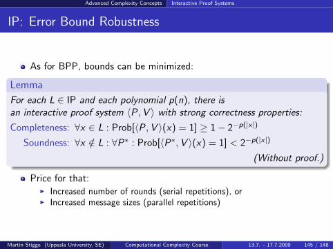
Advanced Complexity Concepts Interactive Proof Systems
IP: Error Bound Robustness
As for BPP, bounds can be minimized:
Lemma
For each L ∈ IP and each polynomial p(n), there isan interactive proof system 〈P,V 〉 with strong correctness properties:
Completeness: ∀x ∈ L : Prob[〈P,V 〉(x) = 1] ≥ 1− 2−p(|x |)
Soundness: ∀x /∈ L : ∀P∗ : Prob[〈P∗,V 〉(x) = 1] < 2−p(|x |)
(Without proof.)
Price for that:I Increased number of rounds (serial repetitions), orI Increased message sizes (parallel repetitions)
Martin Stigge (Uppsala University, SE) Computational Complexity Course 13.7. - 17.7.2009 145 / 148
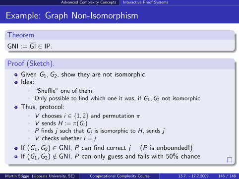
Advanced Complexity Concepts Interactive Proof Systems
Example: Graph Non-Isomorphism
Theorem
GNI := GI ∈ IP.
Proof (Sketch).
Given G1,G2, show they are not isomorphicIdea:
I “Shuffle” one of themI Only possible to find which one it was, if G1,G2 not isomorphic
Thus, protocol:I V chooses i ∈ 1, 2 and permutation πI V sends H := π(Gi )I P finds j such that Gj is isomorphic to H, sends jI V checks whether i = j
If (G1,G2) ∈ GNI, P can find correct j (P is unbounded!)If (G1,G2) /∈ GNI, P can only guess and fails with 50% chance
Martin Stigge (Uppsala University, SE) Computational Complexity Course 13.7. - 17.7.2009 146 / 148
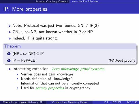
Advanced Complexity Concepts Interactive Proof Systems
IP: More properties
Note: Protocol was just two rounds, GNI ∈ IP(2)
GNI ∈ co- NP, not known whether in P or NP
Indeed, IP is quite strong:
Theorem
1 (NP∪ co- NP) ⊆ IP
2 IP = PSPACE (Without proof.)
Interesting extension: Zero knowledge proof systemsI Verifier does not gain knowledgeI Needs definition of “knowledge”:
Information that can not be efficiently computedI Used for secrecy properties in cryptography
Martin Stigge (Uppsala University, SE) Computational Complexity Course 13.7. - 17.7.2009 147 / 148
Advanced Complexity Concepts Interactive Proof Systems
Course Outline
0 Introduction
1 Basic Computability TheoryFormal LanguagesModel of Computation: Turing MachinesDecidability, Undecidability, Semi-Decidability
2 Complexity ClassesLandau Symbols: The O(·) NotationTime and Space ComplexityRelations between Complexity Classes
3 Feasible Computations: P vs. NPProving vs. VerifyingReductions, Hardness, CompletenessNatural NP-complete problems
4 Advanced Complexity ConceptsNon-uniform ComplexityProbabilistic Complexity ClassesInteractive Proof Systems
Martin Stigge (Uppsala University, SE) Computational Complexity Course 13.7. - 17.7.2009 148 / 148