Real Gas Computation Using an Energy Relaxation …mln/ltrs-pdfs/icase-1998-42.pdf · Real Gas Computation Using an Energy ... need to compute its derivatives or any Riemann ... The

National Aeronautics andSpace Administration

Langley Research CenterHampton, Virginia 23681-2199

NASA/CR-1998-208712ICASE Report No. 98-42

Real Gas Computation Using an Energy RelaxationMethod and High-order WENO Schemes

Philippe Montarnal and Chi-Wang ShuBrown University, Providence, Rhode Island

Institute for Computer Applications in Science and EngineeringNASA Langley Research CenterHampton, VA

Operated by Universities Space Research Association

September 1998

Prepared for Langley Research Centerunder Contract NAS1-97046

REAL GAS COMPUTATION USING AN ENERGY RELAXATIONMETHOD AND HIGH-ORDER WENO SCHEMES

PHILIPPE MONTARNAL ∗ AND CHI-WANG SHU†

Abstract. In this paper, we use a recently developed energy relaxation theory by Coquel and Perthameand high order weighted essentially non-oscillatory (WENO) schemes to simulate the Euler equations ofreal gas. The main idea is an energy decomposition into two parts: one part is associated with a simplerpressure law and the other part (the nonlinear deviation) is convected with the flow. A relaxation process isperformed for each time step to ensure that the original pressure law is satisfied. The necessary characteristicdecomposition for the high order WENO schemes is performed on the characteristic fields based on the firstpart. The algorithm only calls for the original pressure law once per grid point per time step, without theneed to compute its derivatives or any Riemann solvers. Both one and two dimensional numerical examplesare shown to illustrate the effectiveness of this approach.

Key words. Euler equations, real gas, weighted essentially non-oscillatory schemes.

Subject classification. Applied and Numerical Mathematics

1. Introduction. In this paper we consider the Euler equations for a real compressible inviscid fluid,∣∣∣∣∣∣∣∣∣∣∣

∂tρ + div (ρu) = 0, t ≥ 0, x ∈ IRd,

∂tρu + div (ρu⊗ u + p) = 0,

∂tE + div ((E + p)u) = 0,

E =12ρ|u|2 + ρε,

(1.1)

where the quantities ρ, u, p, E and ε represent the density, velocity, pressure, total energy and specific internalenergy, respectively. In addition, there is an equation of state (EOS) of the form p = p(ρ, ε) associated witha strictly convex entropy ρs(ρ, ε) which satisfies the following entropy inequalities

∂tρs + div (ρsu) ≤ 0.(1.2)

The pressure law is furthermore assumed to satisfy

p,ε(ρ, ε) > 0, p(ρ, 0) = 0 and p(ρ,∞) = ∞.(1.3)

In the literature research has been done in order to extend classical schemes designed for perfect gas toreal gases. Collela and Glaz [1] extended the numerical procedure for obtaining the exact Riemann solutionto a real-gas case, Grossman and Walters [7], Liou, van Leer and Shuen [13] extended the method of flux-vector splitting and flux-difference splitting, Montagne, Yee and Vinokur [16] developed second-order explicit

∗Division of Applied Mathematics, Brown University, Providence, RI 02912. Current address: Commissariat a

l’Energie Atomique, Centre d’etude de Bruyeres-le-Chatel, BP 12 - 91680 Bruyeres le Chatel, France. E-mail:

[email protected]. Research supported by an INRIA post-doctoral grant while this author was in residence

at Brown University.†Division of Applied Mathematics, Brown University, Providence, RI 02912. E-mail: [email protected]. Research of this

author was supported in part by ARO grant DAAG55-97-1-0318, NSF grant DMS-9500814, NASA Langley grant NAG-1-

1145 and Contract NAS1-97046 while in residence at ICASE, NASA Langley Research Center, Hampton, VA 23681-2199, and

AFOSR grant F49620-96-1-0150.

1

shock-capturing schemes for real gas, Glaister [5] presented an extension of approximate linearized Riemannsolver with different averaged matrices, while Loh and Liou [15] used the generalization of their Lagrangianapproach (originally proposed for perfect gas) to obtain the real gas Riemann solution.

Most of the previous proposed methods would require a computation of the pressure law and its deriva-tives, or a Riemann solver. This is not only costly but also problematic when there is no analytical expressionsof the pressure law (for example if we have only table values).

Recently Coquel and Perthame [2] have introduced an energy relaxation theory for Euler equations ofreal gas. The main idea is to introduce a relaxation of the nonlinear pressure law by considering an energydecomposition under the form ε = ε1 + ε2. The internal energy ε1 is associated with a simpler pressure lawp1 (which is taken as the γ-law in this paper), while ε2 stands for the nonlinear perturbation and is simplyconvected by the flow. These two energies are also subject to a relaxation process and in the limit of aninfinite relaxation rate, one recovers the initial pressure law p.

From this general framework, Coquel and Perthame have also deduced the extension to general pressurelaws of classical schemes for polytropic gases, which only uses a single call to the pressure law per grid pointand time step. No derivatives of the pressure law or any Riemann solvers need to be computed. Anotheradvantage of their approach is that its implementation does not depend on the particular expression ofthe equation of states. For the first order Godunov scheme, they have shown that this extension satisfiesstability, entropy and accuracy conditions. Numerical examples have been provided using first order schemesby A. In [9].

For Euler equations of polytropic gas, high order ENO (essentially non-oscillatory) and WENO (weightedENO) schemes [8, 18, 19, 20, 14, 10, 21] have been quite successful in providing high resolution results forcomplicated flow structures and shocks. The idea of ENO schemes is to adaptively choose local stencils so thatinterpolation across a discontinuity is avoided as much as possible. WENO uses a nonlinear combination of allstencils to improve upon accuracy and smoothness of numerical fluxes while maintaining the non-oscillatorybehavior of ENO near a discontinuity.

The aim of this paper is to study the implementation of this relaxation method with high order WENOschemes [10] for real gases. One and two dimensional numerical examples will be given.

In Section 2 we provide the general framework of the energy relaxation theory of [2], followed by a shortdescription of high order WENO schemes [10]. We then give the details of the construction of the relaxedWENO schemes for general gases. In Section 3 numerical examples are given. We start with a descriptionof the different equations of states used in this paper, followed by one dimensional shock tube test problems.Two dimensional test cases of a smooth vortex, to test the accuracy of the schemes, and of the double Machreflection problem, are then presented. Concluding remarks are given in Section 4. In the appendices, wegive the expressions of the Roe matrices for the relaxation system (A) and the two molecular vibrating gas(B).

2. Implementation of the energy relaxation method with WENO.

2.1. Energy relaxation theory. The principle of the energy relaxation theory developed by Coqueland Perthame [2] is to find a pressure law p1(ρλ, ελ

1 ) (simpler than p, typically a polytropic law) and aninternal energy φ(ρλ, ελ

1 ) so that the system (1.1) and the entropy inequality (1.2) can be recovered, in thelimit of an infinite relaxation rate λ (called the equilibrium limit), from the following system (called the

2

relaxation system): ∣∣∣∣∣∣∣∣∣∣∣∣∣

∂tρλ + div

(ρλuλ

)= 0, t ≥ 0, x ∈ IRd,

∂tρλuλ + div

(ρλuλ ⊗ uλ + pλ

1

)= 0,

∂tEλ1 + div

((Eλ

1 + pλ1 )uλ

)= λρλ

(ελ2 − φ(ρλ, ελ

1 )),

∂tρλελ

2 + div(ρλuλελ2 ) = −λρλ


1 )),

Eλ1 =

12ρλ|uλ|2 + ρλελ

1 ,

(2.1)

where p1(ρλ, ελ1 ) = (γ1−1)ρλελ

1 with γ1 a given constant greater than 1. One can prove [2] that the relaxationsystem (2.1) can be supplemented by entropy inequalities under the form

∂tρλΣ + div(ρλΣuλ) ≤ REDλ := −λρλ(Σ,s1s1,ε1

− Σ,ε2)(ε2 − φ(ρλ, ελ1 ))

where s1(ρ, ε1) = ργ1−1/ε1 and the specific entropy Σ denotes an arbitrary function in C1(IR2+) such that

ρΣ is convex in (ρ, ρε1, ρε2) and that can be written under the form Σ = Σ(s1(ρ, ε1), ε2). REDλ representsthe Rate of Entropy Dissipation.

Formally, the original Euler system (1.1) will be recovered at λ → +∞ with

ε = ε1 + ε2 = ε1 + φ(ρ, ε1),(2.2)

provided that we have the following condition (called the consistency condition)

p (ρ, ε1 + φ(ρ, ε1)) = p1(ρ, ε1) = (γ1 − 1)ρε1.(2.3)

This last condition can be fulfilled for any given choice of γ1 > 1.But in addition to the conservative system (1.1), one also wants to recover at the limit the entropy

inequality (1.2). The following result, due to Coquel and Perthame [2], gives this last condition under acharacterization of the admissible γ1.

Theorem 2.1. Assuming that γ1 satisfies

γ1 > supρ,ε Γ(ρ, ε) where Γ(ρ, ε) = 1 + p,ε

ρ ,

γ1 > supρ,ε γ(ρ, ε) where γ(ρ, ε) = ρpp,ε + p,ε

ρ ,(2.4)

provided that γ1 is finite, we then have(i) there exists a (unique) specific entropy Σ(s1, ε2) such that at equilibrium (ε = ε1 + φ(ρ, ε1))

s(ρ, ε) = Σ(s1(ρ, ε1), φ(ρ, ε1)),

(ii) this entropy is uniformly compatible with the relaxation procedure, i.e.:

REDλ ≤ 0, for all λ > 0.

2.2. WENO schemes. We use the fifth order WENO scheme in [10]. For a scalar conservation law

ut + f(u)x = 0(2.5)

the derivative f(u)x at the grid point x = xj is approximated by a conservative flux difference

f(u)x|x=xj ≈1

∆x

(fj+ 1

2− fj− 1

2

).(2.6)

3

The WENO numerical flux fj+ 12

is computed as follows. For a positive wind direction f ′(u) ≥ 0, we firstdefine 3 third order numerical fluxes:

f1j+ 1

2=

13f(uj−2)− 7

6f(uj−1) +

116

f(uj),

f2j+ 1

2= −1

6f(uj−1) +

56f(uj) +

13f(uj+1),(2.7)

f3j+ 1

2=

13f(uj) +

56f(uj+1)− 1

6f(uj+2).

A third order ENO scheme will result if we choose one of the three third order fluxes in (2.7) adequately,according to the size of divided differences [19]. On the other hand, a fifth order linear scheme will result ifwe choose the flux as

f linearj+ 1

2= d1f

1j+ 1

2+ d2f

2j+ 1

2+ d3f

3j+ 1

2.(2.8)

with

d1 =110

, d2 =35, d3 =

310

.(2.9)

The fifth order WENO scheme results if we choose the numerical flux as

fj+ 12

= ω1f1j+ 1

2+ ω2f

2j+ 1

2+ ω3f

3j+ 1

2,(2.10)

with ωi defined by

ωi =αi∑3

s=1 αs

, αi =di

(ε + βi)2,(2.11)

and

β1 =1312

(f(ui−2)− 2f(ui−1) + f(ui))2 +14(f(ui−2)− 4f(ui−1) + 3f(ui))2,

β2 =1312

(f(ui−1)− 2f(ui) + f(ui+1))2 +14(f(ui−1)− f(ui+1))2,(2.12)

β3 =1312

(f(ui)− 2f(ui+1) + f(ui+2))2 +14(3f(ui)− 4f(ui+1) + f(ui+2))2.

ε in (2.11) is taken as 10−6 in all our numerical examples, as was done in [10]. The weights in (2.11) arechosen so that in smooth regions (including at smooth extrema), the WENO flux (2.10) behaves similarlyas the linear flux (2.8) and is uniformly fifth order accurate. Near shocks, however, the WENO flux (2.10)behaves similarly as an ENO flux, in the sense that any stencil crossing a discontinuity has a near zeroweight. For details of the derivation, see [10, 21].

If the wind direction is negative, f ′(u) ≤ 0, the procedure is symmetric to the case with f ′(u) ≥ 0, withrespect to the location xj+ 1

2. In general, a flux splitting is used

f(u) = f+(u) + f−(u)(2.13)

such that f+(u) has a positive wind direction and f−(u) has a negative wind direction:

d

duf+(u) ≥ 0,

d

duf−(u) ≤ 0.(2.14)

The procedure described above can then be applied to f+(u) and f−(u) separately. The simplest fluxsplitting is the Lax-Friedrichs splitting:

f±(u) =12

(f(u)± αu)(2.15)

4

where

α = maxu|f ′(u)|.

Notice that while first and second order schemes with a Lax-Friedrichs splitting is quite dissipative, higherorder schemes based on the Lax-Friedrichs fluxes usually give very good results. We use Lax-Friedrichs fluxesin this paper.

For systems of conservation laws in this paper, we use both a component-wise version, where the pro-cedure described above is applied to each equation in the system separately, and a characteristic version,where locally we apply the procedure described above on characteristic projections. For details about howto perform a local characteristic procedure, see for example [18, 19, 10].

2.3. Construction of the relaxed WENO scheme. The procedure to solve the Euler system (1.1)within the framework of the energy relaxation theory is the following. Given the numerical equilibriumsolution at the time level tn

ρ(x, tn), u(x, tn), ε(x, tn),(2.16)

this approximation is advanced to the next time level tn+1 = tn + ∆t in two steps.• First step: relaxation. The two internal energies ε1(x, tn) and ε2(x, tn) are obtained by (2.2) and

the consistency condition (2.3):

ε1(x, tn) =p (ρ(x, tn), ε(x, tn))

(γ1 − 1)ρ(x, tn),

ε2(x, tn) = ε(x, tn)− ε1(x, tn).(2.17)

Notice that this step involves just one call to the pressure law per grid point and does not involveany derivatives of the pressure law or any iterations.

• Second step: evolution in time. For tn ≤ t ≤ tn+1, we solve the Cauchy problem for the relaxationsystem (2.1), with zero on the right side:∣∣∣∣∣∣∣∣∣∣∣∣∣

∂tρλ + div

(ρλuλ

)= 0, t ≥ 0, x ∈ IRd,

∂tρλuλ + div

(ρλuλ ⊗ uλ + pλ

1

)= 0,

∂tEλ1 + div

((Eλ

1 + pλ1 )uλ

)= 0,

∂tρλελ

2 + div(ρλuλελ2 ) = 0,

Eλ1 =

12ρλ|uλ|2 + ρλελ

1 ,

(2.18)

and the initial data

ρ(x, tn), u(x, tn), ε1(x, tn), ε2(x, tn),(2.19)

and we obtain at time tn+1−

ρ(x, tn+1−), u(x, tn+1−), ε1(x, tn+1−), ε2(x, tn+1−).(2.20)

At last, we compute the equilibrium solution at time tn+1 by

ρ(x, tn+1) = ρ(x, tn+1−),u(x, tn+1) = u(x, tn+1−),ε(x, tn+1) = ε1(x, tn+1−) + ε2(x, tn+1−).

(2.21)

5

Remark 1. The first step is clearly a relaxation phase, as it is equivalent to the solution of the followingODE problem for t ≥ tn ∣∣∣∣∣∣∣∣∣∣

dtρλ = 0,

dtρλuλ = 0,

dtEλ1 = λρλ


1 )),

dtρλελ

2 = −λρλ(ελ2 − φ(ρλ, ελ

1 )),

(2.22)

with initial data at time level tn

ρ(x, tn−), u(x, tn−), ε1(x, tn−), ε2(x, tn−).(2.23)

and to let λ → +∞.

We now describe the numerical method we will use for the step of evolution in time. Although ournumerical results concern both one and two dimensional problems, for simplicity of presentations we shallrestrict our description to one space dimension. As we are using the finite difference version of WENOschemes in [10], extensions to two and more spatial dimensions are simply done dimension by dimension.Essentially, the two dimensional code is the one dimensional code with an outside “do loop”.

We have to solve for tn ≤ t < tn+1 the following system of four equations

∂tU + ∂xF (U) = 0,

+ initial conditions given by (2.19),(2.24)

where

U = (ρ, ρu, E1, ρε2)T

,

F (U) =(ρu, ρu2 + p1, (E1 + p1)u, ρuε2

)T.

(2.25)

In order to solve the ordinary differential equation

d

dtU = L(U),(2.26)

where L(U) is a discretization of the spatial operator, we use a third-order TVD Runge-Kutta scheme [18].Remark 2. We have two possibilities for the placement of the relaxation step: each Runge-Kutta

inner stage or each time step. With the first example of section 3.3, we show that the two approaches givenearly identical results in accuracy. Of course the second approach is less costly. We thus perform all ourcalculations using the second approach.

We now discretize the space into uniform intervals of size ∆x and denote xj = j∆x. Various quantitiesat xj will be identified by the subscript j.

We use the WENO procedure described in the previous subsection to obtain the spatial operator Lj(U)which approximates −∂xF (U) at xj . We have tested several possibilities for the definition of L(U) basedon WENO schemes. The first one is to use a WENO Lax-Friedrichs scheme with a full characteristicdecomposition. For this purpose we need to compute a Roe matrix for the system (2.24) and its eigenvaluesand eigenvectors. The details of this derivation are included in Appendix A.

The other possibility is to compute the first three components of the numerical flux F 1j+ 1

2, F 2

j+ 12, F 3

j+ 12

by using a WENO Lax-Friedrichs scheme with a decomposition on the Euler system characteristics and toobtain the last numerical flux F 4

j+ 12

with a scalar WENO Lax-Friedrichs scheme. This is possible becausethe first three equations of system (2.24) are independent from the last one.

6

Remark 3. We have also tried to compute the last numerical flux by using a first order scheme speciallydesigned in order to preserve the maximum principle for ε2 [11]. But with this approach, we lose the accuracyof the high-order WENO scheme also for the other variables.

Remark 4. In order to make comparisons in the numerical results we have also implemented a WENOLax-Friedrichs scheme with a full characteristic decomposition for a two molecular vibrating gas (see nextsection for a description of the related EOS). For this purpose we need a definition of the corresponding Roeaverage matrix. We give it in Appendix B. For the numerical comparisons for the other real gases we use acomponent-wise WENO Lax-Friedrichs scheme which requires only the computation of the sound velocity

c =√

p,ρ + pp,ε

ρ2.(2.27)

3. Numerical results.

3.1. Description of the different equations of states. We present here several equations of stateswhich we will use in the computation. We find the second one in the paper of In [9], while the third onecomes from Glaister [4]).

• Polytropic ideal gas. The equation of states for a polytropic ideal gas (also called perfect gas) is thefollowing

p(ρ, ε) = (γ − 1)ρε.(3.1)

Then we have

p,ρ = (γ − 1)ε, p,ε = (γ − 1)ρ.(3.2)

Air under normal conditions (p and T moderate enough) can be considered as a perfect gas with γ = 7/5 = 1.4(approximately a mixture of two diatomic molecular species: 20% of O2, 80% of N2).

• Two molecular vibrating gas. When the temperature increases the vibrational motion of oxygen andnitrogen molecules in air becomes important, and specific heats vary with temperatures. So that one mustconsider the following thermally perfect, calorically imperfect model for two molecular vibrating gas

p(ρ, ε) = rρT (ε)(3.3)

where the temperature T is given by the implicit expression

ρε = ctrv T + ρ

αΘvib

exp(

Θvib

T

)− 1,(3.4)

with r = 287.086 J · kg−1 ·K−1, Ctrv = r/(γtr − 1), γtr = 1.4, Θvib = 103 K, α = r. Then we have

p,ρ = rT (ε), p,ε =rρ

ε′(T (ε)).(3.5)

• Osborne model. R. K. Osborne from the Los Alamos Scientific Laboratory has developed a quitegeneral equation of states in the following form [17]

p(ρ, ε) =1

E + φ0(ζ(a1 + a2ζ) + E (b0 + ζ(b1 + b2ζ) + E(c0 + c1ζ)))(3.6)

7

where E = ρ0ε and ζ = ρρ0− 1 and the constants ρ0, a1, a2, b0, b1, b2, c0, c1, φ0 depend on the material in

question. The typical values for water are ρ0 = 10−2, a1 = 3.84×10−4, a2 = 1.756×10−3, b0 = 1.312×10−2,b1 = 6.265× 10−2, b2 = 0.2133, c0 = 0.5132, c1 = 0.6761 and φ0 = 2.× 10−2. Then we have

p,ρ = 1ρ0(E+φ0)

((a1 + 2a2ζ) + E (b1 + 2b2ζ + Ec1)) ,

p,ε = − ρ0E+φ0

p + ρ0E+φ0

(b0 + ζ(b1 + b2ζ) + 2E(c0 + c1ζ)) .

(3.7)

3.2. One dimension cases.

• Example 1. 1D Riemann problems with perfect gas.We consider here two well-known problems which have the following Riemann type initial conditions:

u(x, 0) =

{uL if x < 0,

uR if x > 0.

The first one is Sod’s problem [22]. The initial data are

(ρL, uL, pL) = (1, 0, 1), (ρR, uR, pR) = (0.125, 0, 0.1).

The second one is proposed by Lax [12] with

(ρL, uL, pL) = (0.445, 0.698, 3.528), (ρR, uR, pR) = (0.5, 0, 0.571).

Of course for this perfect gas situation there is no need to use the relaxation model in practice. Thepurpose of this test problem is to test the behavior of different relaxation models (different γ1’s) and differ-ent ways of treating the relaxed system (fully characteristic and partially characteristic for the first threeequations only).

For this example, a uniform grid of 100 points are used and every 2 points are drawn in the figures.We first give, in Table 3.1, a CPU time comparison among the traditional WENO characteristic scheme

for the perfect gas, and the WENO scheme applied to the relaxation system, both with a fully characteristicdecomposition and with a partially characteristic decomposition for the first three equations only. Thecalculation is done on a SUN Ultra1 workstation. We can see that while a fully characteristic decompositionis significantly more costly, the partially characteristic decomposition is only slightly more costly than theWENO scheme applied to the original perfect gas Euler equations.

Case WENO Relaxed WENO with Relaxed WENO withwith characteristic full characteristic partial characteristic

Sod Shock 2.28 3.49 2.91

Lax Shock 3.32 4.93 4.08Table 3.1

CPU time (in seconds) of different schemes for the Sod and Lax shock tube problems for a perfect gas.

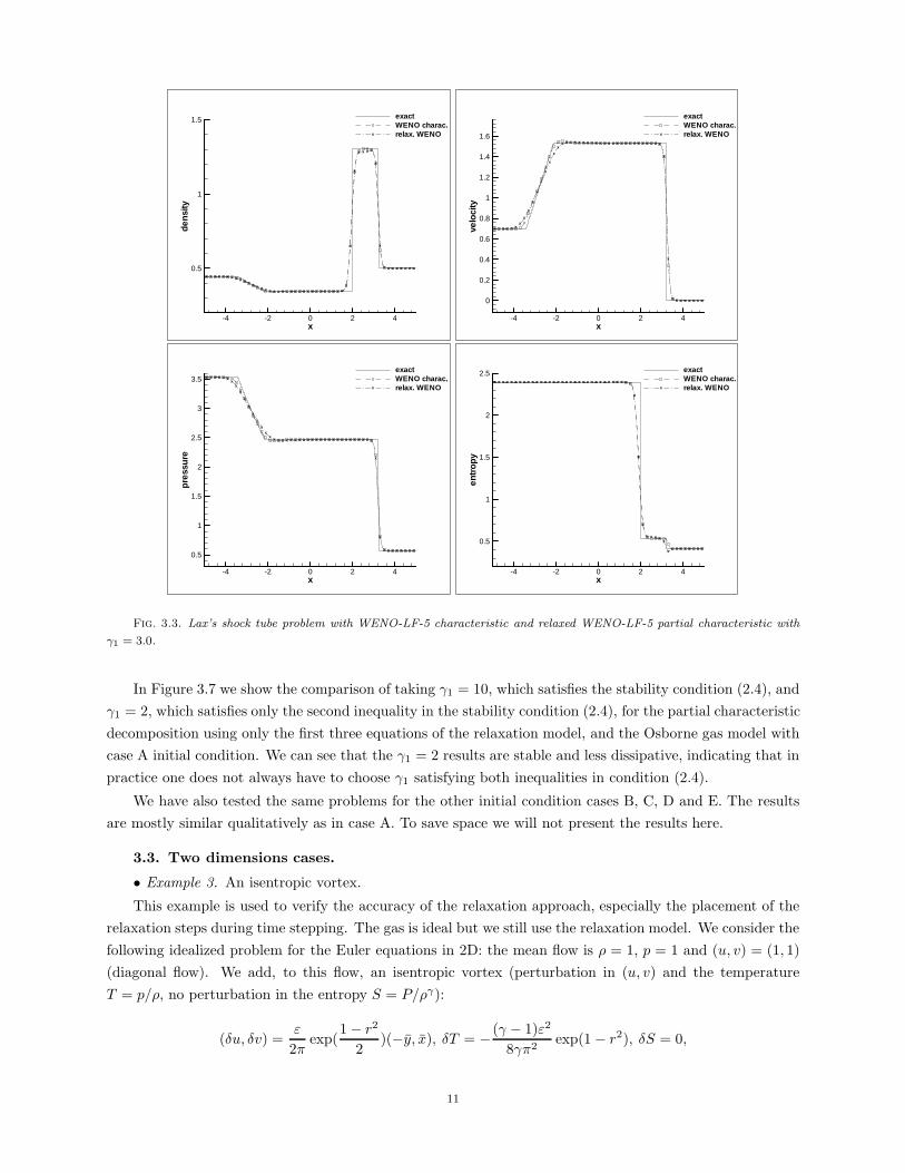
In Figures 3.1 and 3.3, we present the comparison for the Sod’s and Lax’s shock tube problems, of thefifth order WENO schemes, applied directly to the perfect gas Euler equations using a characteristic decom-position, and applied to the relaxation model with γ1 = 3 using only partial characteristic decomposition ofthe first 3 equations. We can see that the results are very close, except for the slight over- and under-shootsin entropy for the relaxation model calculation. This indicates the feasibility of using the relaxation model.

8

-4 -2 0 2 4x

0

0.1

0.2

0.3

0.4

0.5

0.6

0.7

0.8

0.9

1

1.1

den

sity

X X X X X X X X X X X XX

X

X

X

X

X

X

X

X

X

X

XX

X X X X X X X X

X

XX X X X X X X

X

X X X X X X X

exactWENO charac.relax. WENOX

-4 -2 0 2 4x

0

0.1

0.2

0.3

0.4

0.5

0.6

0.7

0.8

0.9

1

1.1

velo

city


X

X

X

X

X

X

X

X

X

X

X

XX X X X X X X X X X X X X X X X

X

X

XX X X X X X


-4 -2 0 2 4x

0

0.1

0.2

0.3

0.4

0.5

0.6

0.7

0.8

0.9

1

pre

ssu

re

X X X X X X X X X X XX

X

X

X

X

X

X

X

X

X

X

X

X

XX X X X X X X X X X X X X X X X X

X

X X X X X X X


-4 -2 0 2 4x

0

0.1

0.2

0.3

0.4

0.5

0.6

0.7

0.8

entr

opy

X X X X X X X X X X X X X X X X X X X X X X X X X X X X X X X XX

X

X

X XX X X X X

XX X X X X X X


Fig. 3.1. Sod’s shock tube problem with WENO-LF-5 characteristic and relaxed WENO-LF-5 partial characteristic with

γ1 = 3.0.

In Figures 3.2 and 3.4, we present the comparison for the Sod’s and Lax’s shock tube problems, ofthe fifth order WENO schemes. The top left figure compares the full characteristic decomposition for therelaxation model, with a partial characteristic decomposition for the first 3 equations only, for γ1 = 3.We can see that the results are quite close, again indicating the feasibility of using the less costly partialcharacteristic decomposition for the relaxation model. The top right figure compares the effect of different γ1’sin the relaxation model. Apparently bigger γ1 corresponds to larger numerical dissipation. This indicatesthat one should always choose the smallest possible γ1 subject to stability considerations. The bottomfigure compares the relaxation WENO results for γ1 = 3 and a partial characteristic decomposition, witha component-wise WENO scheme applied directly on the original perfect gas Euler equations. Althoughneither uses the correct characteristic information, apparently the relaxation model results are better thanthe component-wise results, especially for the Lax’s problem in Figure 3.4.

• Example 2. 1D Riemann problems with real gases.

In this example we compute the solutions to the Riemann shock tube problem, for the two molecularvibrating gas (3.3)-(3.5) and the Osborne model (3.6)-(3.7), with the following initial conditions in Table3.2.

For this example, a uniform grid of 200 points are used and every 4 points are drawn in the figures.

9

-4 -2 0 2 4x

0

0.1

0.2

0.3

0.4

0.5

0.6

0.7

0.8

0.9

1

1.1

den

sity


X

X

X

X

X

X

X

X

X

X

XX

X X X X X X X X

X

X

X X X X X X X

X

X X X X X X X

exactpartial charac.full charac.X

(a)

-4 -2 0 2 4x

0

0.1

0.2

0.3

0.4

0.5

0.6

0.7

0.8

0.9

1

1.1

den

sity

X X X X X X X X X XX

XX

X

X

X

X

X

X

X

X

X

X

X

XX

XX X X X X

X

X

X X X X X X X

X

X

X X X X X X X

exactgamma1=3.0gamma1=30.0X

(b)

-4 -2 0 2 4x

0

0.1

0.2

0.3

0.4

0.5

0.6

0.7

0.8

0.9

1

1.1

den

sity


X

X

X

X

X

X

X

X

X

X

XX

X X X X X X X X

X

XX X X X X X X

X

X X X X X X X

exactWENO compo.relax. WENOX

(c)

Fig. 3.2. Sod’s shock tube problem with WENO-LF-5. Comparisons of partial and full characteristic decompositions for

the relaxation model with γ1 = 3 (top left); γ1 = 3 and γ1 = 30 for the relaxation model with partial characteristic decomposition

(top right); and the relaxation model with partial characteristic decomposition with γ1 = 3 versus the component-wise WENO

applied to the original perfect gas Euler equations.

Also, the “exact solution” in the figures are obtained with the best scheme using 2000 points.We first give a CPU time comparison between the full characteristic decomposition for the original model

and the partial characteristic decomposition using only the first three equations of the relaxation model, forthe two molecular vibrating gas model, in Table 3.3. We can see that the partial characteristic decompositionfor the relaxed model is usually more than twice less costly than the full characteristic version for the originalsystem. Although the relaxed model has one more equation, it does not require the computation of thecomplicated derivatives of the EOS.

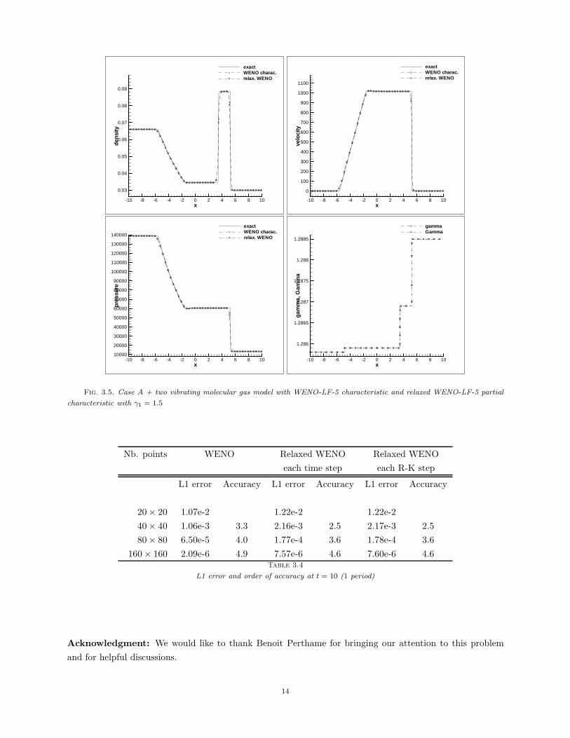
In Figure 3.5 we show the comparison of the full characteristic decomposition for the original model andthe partial characteristic decomposition using only the first three equations of the relaxation model, for thetwo molecular vibrating gas model, with case A initial condition. The results are almost identical, indicatingthat the relaxation model with a partial characteristic decomposition works well with a much reduced cost.

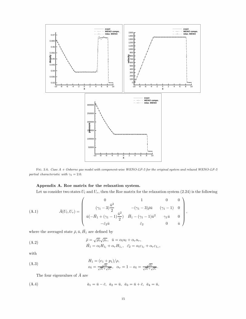
In Figure 3.6 we show the comparison of the component WENO scheme on the original system, and thepartially characteristic WENO scheme on the relaxed system with γ1 = 2.0, for the Osborne gas model withcase A initial condition. We can see that the result of the relaxed model is much better, especially for thedensity. This indicates that the relaxation model is a good one for the computation of real gases.

10

-4 -2 0 2 4x

0.5

1

1.5

den

sity

X X X X X X X X X X X X X X X X X X X X X X X X X X X X X X X X X

X

X

X

X X X X

X

X

X X X X X X X X


-4 -2 0 2 4x

0

0.2

0.4

0.6

0.8

1

1.2

1.4

1.6

velo

city

X X X X X XX

X

X

X

X

X

X

X

X

XX X X X X X X X X X X X X X X X X X X X X X X X

X

X

X X X X X X X X


-4 -2 0 2 4x

0.5

1

1.5

2

2.5

3

3.5

pre

ssu

re

X X X X X XX

X

X

X

X

X

X

X

XX

X X X X X X X X X X X X X X X X X X X X X X X X

X

X

X X X X X X X X


-4 -2 0 2 4x

0.5

1

1.5

2

2.5

entr

opy


X

X

X

X X X XX

XX X X X X X X X


Fig. 3.3. Lax’s shock tube problem with WENO-LF-5 characteristic and relaxed WENO-LF-5 partial characteristic with

γ1 = 3.0.

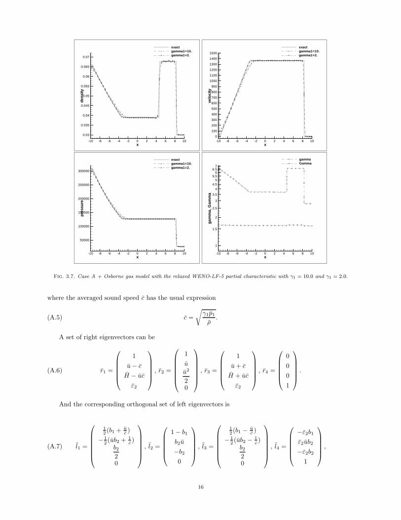
In Figure 3.7 we show the comparison of taking γ1 = 10, which satisfies the stability condition (2.4), andγ1 = 2, which satisfies only the second inequality in the stability condition (2.4), for the partial characteristicdecomposition using only the first three equations of the relaxation model, and the Osborne gas model withcase A initial condition. We can see that the γ1 = 2 results are stable and less dissipative, indicating that inpractice one does not always have to choose γ1 satisfying both inequalities in condition (2.4).

We have also tested the same problems for the other initial condition cases B, C, D and E. The resultsare mostly similar qualitatively as in case A. To save space we will not present the results here.

3.3. Two dimensions cases.

• Example 3. An isentropic vortex.

This example is used to verify the accuracy of the relaxation approach, especially the placement of therelaxation steps during time stepping. The gas is ideal but we still use the relaxation model. We consider thefollowing idealized problem for the Euler equations in 2D: the mean flow is ρ = 1, p = 1 and (u, v) = (1, 1)(diagonal flow). We add, to this flow, an isentropic vortex (perturbation in (u, v) and the temperatureT = p/ρ, no perturbation in the entropy S = P/ργ):

(δu, δv) =ε

2πexp(

1− r2

2)(−y, x), δT = − (γ − 1)ε2

8γπ2exp(1− r2), δS = 0,

11

-4 -2 0 2 4x

0.5

1

1.5

den

sity


X

X

X

X X X X

X

X

X X X X X X X X

exactpartial charac.full charac.X

(a)

-4 -2 0 2 4x

0.5

1

1.5

den

sity


X

X

X

X X XX

X

X

X

X X X X X X X

exactgamma1=3.0gamma1=30.0X

(b)

-4 -2 0 2 4x

0.5

1

1.5

den

sity


X

X

X

X X X X

X

X

X X X X X X X X


(c)

Fig. 3.4. Lax’s shock tube problem with WENO-LF-5. Comparisons of partial and full characteristic decompositions for

the relaxation model with γ1 = 3 (top left); γ1 = 3 and γ1 = 30 for the relaxation model with partial characteristic decomposition

(top right); and the relaxation model with partial characteristic decomposition with γ1 = 3 versus the component-wise WENO

applied to the original perfect gas Euler equations.

where (x, y) = (x − 5, y − 5), r2 = x2 + y2, and the vortex strength ε = 5. See [21].The computational domain is taken as [0, 10, ]× [0, 10], extended periodically in both directions. This

allows us to perform long time simulation without having to deal with a large domain.It is clear that the exact solution of the Euler equation with the above initial and boundary conditions

is just the passive convection of the vortex with the mean velocity.In Table 3.4 we show the accuracy result at t = 10 (one time period). We can see that WENO for the

relaxed model with γ1 = 3 gives a somewhat larger error than WENO applied directly to the original system,but the order of accuracy is correct. Moreover, to place the relaxation step for each Runge-Kutta inner stageor just for each time step seems to give almost identical results. We have thus used the less costly version ofputting the relaxation step for every time step in all the numerical examples in this paper.

• Example 4. Double Mach reflection.The computational domain is chosen to be [0, 4]× [0, 1], although only part of it ([0, 3]× [[0, 1]) is shown.

The reflecting wall lies at the bottom of the computational domain starting from x = 1/6. Initially a right-moving Mach 10 shock is positioned at (x, y) = (1/6, 0) and makes a 60◦ angle with the x-axis. For thebottom boundary, the exact post-shock condition is imposed for the part from x = 0 to x = 1/6 and a

12

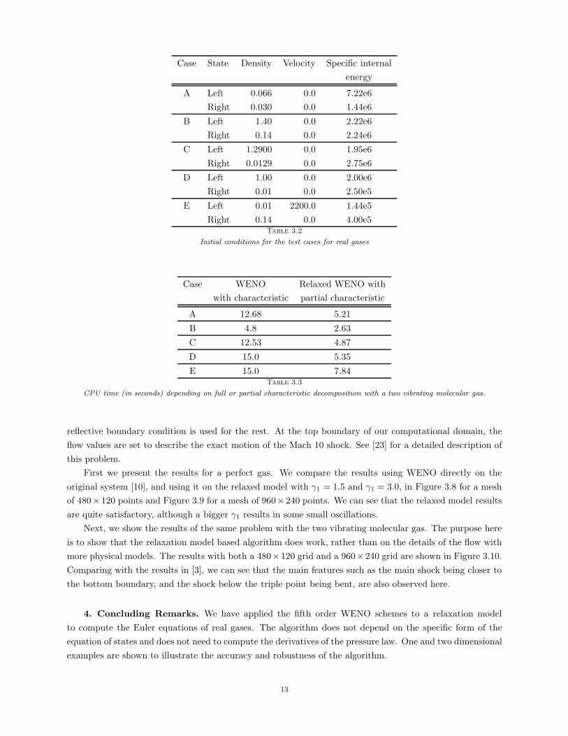
Case State Density Velocity Specific internalenergy

A Left 0.066 0.0 7.22e6Right 0.030 0.0 1.44e6

B Left 1.40 0.0 2.22e6Right 0.14 0.0 2.24e6

C Left 1.2900 0.0 1.95e6Right 0.0129 0.0 2.75e6

D Left 1.00 0.0 2.00e6Right 0.01 0.0 2.50e5

E Left 0.01 2200.0 1.44e5Right 0.14 0.0 4.00e5

Table 3.2

Initial conditions for the test cases for real gases

Case WENO Relaxed WENO withwith characteristic partial characteristic

A 12.68 5.21

B 4.8 2.63

C 12.53 4.87

D 15.0 5.35

E 15.0 7.84Table 3.3

CPU time (in seconds) depending on full or partial characteristic decomposition with a two vibrating molecular gas.

reflective boundary condition is used for the rest. At the top boundary of our computational domain, theflow values are set to describe the exact motion of the Mach 10 shock. See [23] for a detailed description ofthis problem.

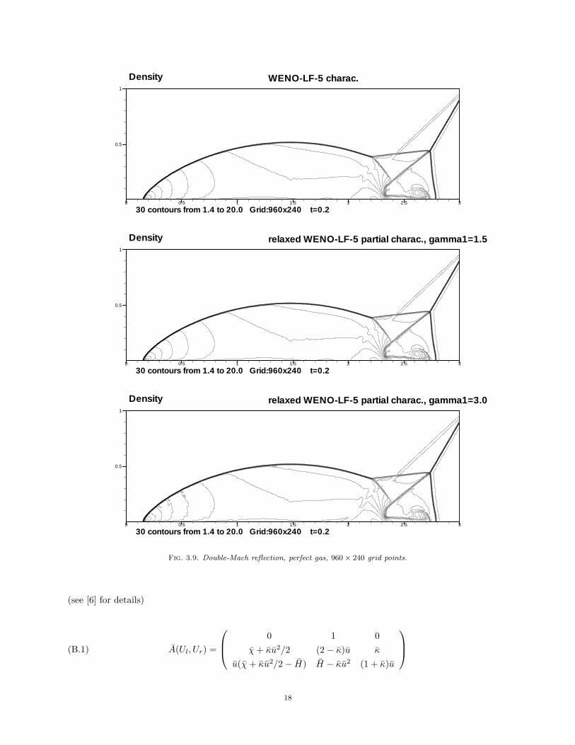
First we present the results for a perfect gas. We compare the results using WENO directly on theoriginal system [10], and using it on the relaxed model with γ1 = 1.5 and γ1 = 3.0, in Figure 3.8 for a meshof 480× 120 points and Figure 3.9 for a mesh of 960× 240 points. We can see that the relaxed model resultsare quite satisfactory, although a bigger γ1 results in some small oscillations.

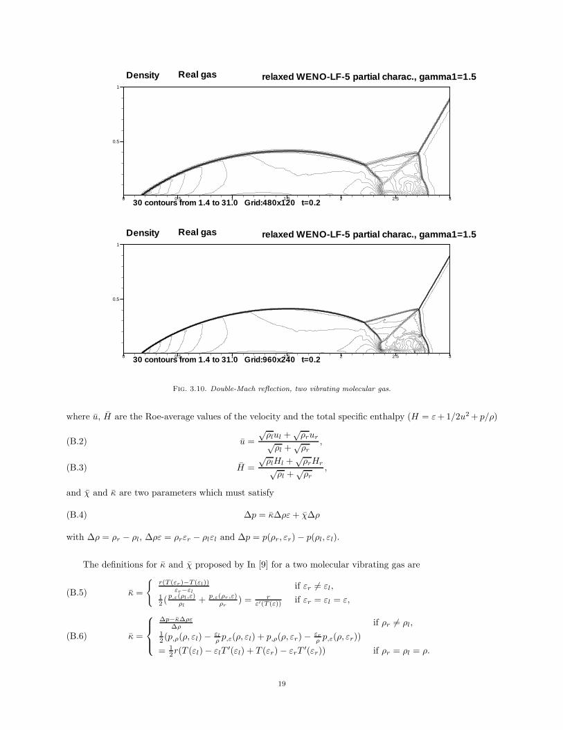
Next, we show the results of the same problem with the two vibrating molecular gas. The purpose hereis to show that the relaxation model based algorithm does work, rather than on the details of the flow withmore physical models. The results with both a 480×120 grid and a 960×240 grid are shown in Figure 3.10.Comparing with the results in [3], we can see that the main features such as the main shock being closer tothe bottom boundary, and the shock below the triple point being bent, are also observed here.

4. Concluding Remarks. We have applied the fifth order WENO schemes to a relaxation modelto compute the Euler equations of real gases. The algorithm does not depend on the specific form of theequation of states and does not need to compute the derivatives of the pressure law. One and two dimensionalexamples are shown to illustrate the accuracy and robustness of the algorithm.

13

-10 -8 -6 -4 -2 0 2 4 6 8 10x

0.03

0.04

0.05

0.06

0.07

0.08

0.09

den

sity X X X X X X X X X X

X

X

X

X

X

X

X

X

X

X

XX X X X X X X X X X X

X

X

X X X

X

X X X X X X X X X X X X


-10 -8 -6 -4 -2 0 2 4 6 8 10x

0

100

200

300

400

500

600

700

800

900

1000

1100

velo

city


X

X

X

X

X

X

X

X

X

X

X X X X X X X X X X X X X X X X

X



-10 -8 -6 -4 -2 0 2 4 6 8 10x

10000

20000

30000

40000

50000

60000

70000

80000

90000

100000

110000

120000

130000

140000

pre

ssu

re


X

X

X

X

X

X

X

X

X

XX X X X X X X X X X X X X X X X

X



-10 -8 -6 -4 -2 0 2 4 6 8 10x

1.286

1.2865

1.287

1.2875

1.288

1.2885

gam

ma,

Gam

ma

X X X X X X X

X X X X X X X X X X X

X

X

X

X

X

X X

X

X

X

X

X X X X X X

gammaGammaX

Fig. 3.5. Case A + two vibrating molecular gas model with WENO-LF-5 characteristic and relaxed WENO-LF-5 partial

characteristic with γ1 = 1.5

Nb. points WENO Relaxed WENO Relaxed WENOeach time step each R-K step

L1 error Accuracy L1 error Accuracy L1 error Accuracy

20× 20 1.07e-2 1.22e-2 1.22e-240× 40 1.06e-3 3.3 2.16e-3 2.5 2.17e-3 2.580× 80 6.50e-5 4.0 1.77e-4 3.6 1.78e-4 3.6

160× 160 2.09e-6 4.9 7.57e-6 4.6 7.60e-6 4.6Table 3.4

L1 error and order of accuracy at t = 10 (1 period)

Acknowledgment: We would like to thank Benoit Perthame for bringing our attention to this problemand for helpful discussions.

14

-10 -8 -6 -4 -2 0 2 4 6 8 10x

0.03

0.035

0.04

0.045

0.05

0.055

0.06

0.065

0.07

den

sity

X

X

X

X

X

X

X

X

X

X

X

X

X

X

X

XX

X X X X X X X X X X X X X X X X X XX

X

X X X X X X X X

X

X X X X


-10 -8 -6 -4 -2 0 2 4 6 8 10x

0

100

200

300

400

500

600

700

800

900

1000

1100

1200

1300

1400

1500

velo

city

X

X

X

X

X

X

X

X

X

X

X

X

X

X

X

X

XX X X X X X X X X X X X X X X X X X X X X X X X X X X X

X

X X X X


-10 -8 -6 -4 -2 0 2 4 6 8 10x

50000

100000

150000

200000

250000

300000

pre

ssu

re

X

X

X

X

X

X

X

X

X

X

X

X

X

X

XX

X X X X X X X X X X X X X X X X X X X X X X X X X X X X X

X

X X X X


Fig. 3.6. Case A + Osborne gas model with component-wise WENO-LF-5 for the original system and relaxed WENO-LF-5

partial characteristic with γ1 = 2.0.

Appendix A. Roe matrix for the relaxation system.

Let us consider two states Ul and Ur, then the Roe matrix for the relaxation system (2.24) is the following

A(Ul, Ur) =

0 1 0 0

(γ1 − 3)u2

2−(γ1 − 3)ρu (γ1 − 1) 0

u(−H1 + (γ1 − 1)u2

2) H1 − (γ1 − 1)u2 γ1u 0

−ε2u ε2 0 u

,(A.1)

where the averaged state ρ, u, H1 are defined by

ρ =√

ρl√

ρr, u = αlul + αrur,

H1 = αlH1l+ αrH1r , ε2 = αlε1l

+ αrε1r ,(A.2)

with

H1 = (e1 + p1)/ρ,

αl =√

ρl√ρl+

√ρr

, αr = 1− αl =√

ρr√ρl+

√ρr

.(A.3)

The four eigenvalues of A are

a1 = u− c, a2 = u, a3 = u + c, a4 = u,(A.4)

15

-10 -8 -6 -4 -2 0 2 4 6 8 10x

0.03

0.035

0.04

0.045

0.05

0.055

0.06

0.065

0.07

den

sity

X

X

X

X

X

X

X

X

X

X

X

X

X

X

X

XX

X X X X X X X X X X X X X X X X X XX

X

X X X X X X X X

X

X X X X

exactgamma1=10.gamma1=2.X

-10 -8 -6 -4 -2 0 2 4 6 8 10x

0

100

200

300

400

500

600

700

800

900

1000

1100

1200

1300

1400

1500

velo

city

X

X

X

X

X

X

X

X

X

X

X

X

X

X

X

X

XX X X X X X X X X X X X X X X X X X X X X X X X X X X X

X

X X X X


-10 -8 -6 -4 -2 0 2 4 6 8 10x

50000

100000

150000

200000

250000

300000

pre

ssu

re

X

X

X

X

X

X

X

X

X

X

X

X

X

X

XX

X X X X X X X X X X X X X X X X X X X X X X X X X X X X X

X

X X X X


-10 -8 -6 -4 -2 0 2 4 6 8 10x

1

1.5

2

2.5

3

3.5

44.5

55.5

66.5

7

gam

ma,

Gam

ma

X X X X X X X X X X X X X X X X X X X X X X X X X X

gammaGammaX

Fig. 3.7. Case A + Osborne gas model with the relaxed WENO-LF-5 partial characteristic with γ1 = 10.0 and γ1 = 2.0.

where the averaged sound speed c has the usual expression

c =√

γ1p1

ρ.(A.5)

A set of right eigenvectors can be

r1 =

1u− c

H − uc

ε2

, r2 =

1u

u2

20

, r3 =

1u + c

H + uc

ε2

, r4 =

0001

.(A.6)

And the corresponding orthogonal set of left eigenvectors is

l1 =

12 (b1 + u

c )− 1

2 (ub2 + 1c )

b2

20

, l2 =

1− b1

b2u

−b2

0

, l3 =

12 (b1 − u

c )− 1

2 (ub2 − 1c )

b2

20

, l4 =

−ε2b1

ε2ub2

−ε2b2

1

,(A.7)

16

0 0.5 1 1.5 2 2.5 3

0.5

1

Density WENO-LF-5 charac.

30 contours from 1.4 to 20.0 Grid:480x120 t=0.2

0 0.5 1 1.5 2 2.5 3

0.5

1

Density relaxed WENO-LF-5 partial charac., gamma1=1.5


0 0.5 1 1.5 2 2.5 3

0.5

1



Fig. 3.8. Double-Mach reflection, perfect gas, 480× 120 grid points.

where

b1 =(γ1 − 1)u2

2c2, b2 =

(γ1 − 1)c2

.(A.8)

Appendix B. Roe matrix for a two molecular vibrating gas.

Let us consider two states Ul and Ur, then the Roe matrix for an Euler system of real gas is the following

17

0 0.5 1 1.5 2 2.5 3

0.5

1

Density WENO-LF-5 charac.


0 0.5 1 1.5 2 2.5 3

0.5

1



0 0.5 1 1.5 2 2.5 3

0.5

1



Fig. 3.9. Double-Mach reflection, perfect gas, 960× 240 grid points.

(see [6] for details)

A(Ul, Ur) =

0 1 0χ + κu2/2 (2 − κ)u κ

u(χ + κu2/2− H) H − κu2 (1 + κ)u

(B.1)

18

0 0.5 1 1.5 2 2.5 3

0.5

1



Real gas

0 0.5 1 1.5 2 2.5 3

0.5

1



Real gas

Fig. 3.10. Double-Mach reflection, two vibrating molecular gas.

where u, H are the Roe-average values of the velocity and the total specific enthalpy (H = ε + 1/2u2 + p/ρ)

u =√

ρlul +√

ρrur√ρl +

√ρr

,(B.2)

H =√

ρlHl +√

ρrHr√ρl +

√ρr

,(B.3)

and χ and κ are two parameters which must satisfy

∆p = κ∆ρε + χ∆ρ(B.4)

with ∆ρ = ρr − ρl, ∆ρε = ρrεr − ρlεl and ∆p = p(ρr, εr)− p(ρl, εl).

The definitions for κ and χ proposed by In [9] for a two molecular vibrating gas are

κ =

{r(T (εr)−T (εl))

εr−εlif εr 6= εl,

12 (p,ε(ρl,ε)

ρl+ p,ε(ρr ,ε)

ρr) = r

ε′(T (ε)) if εr = εl = ε,(B.5)

κ =

∆p−κ∆ρε∆ρ if ρr 6= ρl,

12 (p,ρ(ρ, εl)− εl

ρ p,ε(ρ, εl) + p,ρ(ρ, εr)− εr

ρ p,ε(ρ, εr))

= 12r(T (εl)− εlT

′(εl) + T (εr)− εrT′(εr)) if ρr = ρl = ρ.

(B.6)

19

The definitions of the eigenvalues and right and left eigenvectors are easy to obtain and are omittedhere.

REFERENCES

[1] P. Colella and H. M. Glaz, Efficient solution algorithms for the Riemann problem for real gases,J. Comput. Phys., 59 (1985), pp. 264–289.

[2] F. Coquel and B. Perthame, Relaxation of energy and approximate Riemann solvers for generalpressure laws in fluid dynamics equations, SIAM J. Numer. Anal., to appear.

[3] R.L. Deschambault and I.I. Glass, An update on non-stationary oblique shock-wave reflections:Actual isopycnics and numerical experiments, J. Fluid Mech., 131 (1983), pp. 27–57.

[4] P. Glaister, An efficient numerical method for compressible flows of a real gas using arithmeticaveraging, Comput. Math. Appl., 28 (1994), pp. 97–113.

[5] , An analysis of averaging procedures in a Riemann solver for compressible flows of a real gas,Comput. Math. Appl., 33 (1997), pp. 105–119.

[6] E. Godlewski and P.-A. Raviart, Numerical approximation of hyperbolic systems of conservationlaws, Springer, 1996.

[7] B. Grossman and R. W. Walters, Analysis of flux-split algorithms for Euler’s equations with realgases, AIAA J., 27 (1989), pp. 524–531.

[8] A. Harten, B. Engquist, S. Osher and S. Chakravarthy, Uniformly high order essentially non-oscillatory schemes, III, J. Comput. Phys., 71 (1987), pp. 231–303.

[9] A. In, Numerical evaluation of an energy relaxation method for inviscid real fluids, EDF research reportHT-13/97/032/A, submitted for publication.

[10] G.-S. Jiang and C.-W. Shu, Efficient implementation of weighed ENO schemes, J. Comput. Phys.,126 (1996), pp. 202–228.

[11] B. Larrouturou, How to preserve the mass fractions positivity when computing compressible multi-component flows, J. Comput. Phys., 95 (1991), pp. 59–84.

[12] P. D. Lax, Weak solutions of non-linear hyperbolic equations and their numerical computations, Com-mmun. Pure Appl. Math., 7 (1954), pp. 159–193.

[13] M. S. Liou, B. van Leer, and J.-S. Shuen, Splitting of inviscid fluxes for real gases, J. Comput.Phys., 87 (1990), pp. 1–24.

[14] X.-D. Liu, S. Osher, and T. Chan, Weighed essentially non-oscillatory schemes, J. Comput. Phys.,115 (1994), pp. 200–212.

[15] C.-Y. Loh and M. S. Liou, Lagrangian solution of supersonic real gas flows, J. Comput. Phys., 104(1993), pp. 150–161.

[16] J.-L. Montagne, H. C. Yee, and M. Vinokur, Comparative study of high-resolution shock-capturingschemes for a real gas, AIAA Journal, 27 (1989), pp. 1332–1346.

[17] T. D. Riney, Numerical evaluation of hypervelocity impact phenomena, in High-velocity impact phe-nomena, R. Kinslow, ed., Academic Press, 1970, ch. V, pp. 158–212.

[18] C.-W. Shu and S. Osher, Efficient implementation of essentially non-oscillatory shock-capturingschemes, J. Comput. Phys., 77 (1988), pp. 439–471.

[19] C.-W. Shu and S. Osher, Efficient implementation of essentially non-oscillatory shock-capturingschemes, II, J. Comput. Phys., 83 (1989), pp. 32–78.

20

[20] C.-W. Shu, T.A. Zang, G. Erlebacher, D. Whitaker, and S. Osher, High order ENO schemesapplied to two- and three- dimensional compressible flow, Appl. Numer. Math., 9 (1992), pp. 45–71.

[21] C.-W. Shu, Essentially non-oscillatory and weighted essentially non-oscillatory schemes for hyperbolicconservation laws, in Advanced Numerical Approximation of Nonlinear Hyperbolic Equations, A.Quarteroni, Editor, Lecture Notes in Mathematics, CIME subseries, Springer-Verlag, to appear.

[22] G. Sod, A survey of several finite difference methods for systems of non-linear hyperbolic conservationlaws, J. Comput. Phys., 27 (1978).

[23] P. Woodward and P. Colella, The numerical simulation of two-dimensional fluid flow with strongshocks, J. Comput. Phys., 54 (1984), pp. 125–160.

21

Documents

Real Gas Computation Using an Energy Relaxation …mln/ltrs-pdfs/icase-1998-42.pdf · Real Gas Computation Using an Energy ... need to compute its derivatives or any Riemann ... The