Vol. 7(4), pp. 80-97, April, 2015

DOI: 10.5897/JEIF2014.0631

Article Number: 110EA8A52525

ISSN 2141-6672

Copyright © 2015

Author(s) retain the copyright of this article

http://www.academicjournals.org/JEIF

Journal of Economics and International Finance

Full Length Research Paper

Real exchange rate assessment in Egypt: Equilibrium and misalignments

Rana Hosni1* and Dina Rofael2

1Economics Department, Faculty of Economics and Political Science, Cairo University.

2Monetary Policy Department, Central Bank of Egypt.

Received 10 December, 2014; Accepted 26 March, 2015

The underlying study focuses on assessing the real exchange rate in Egypt during the period 1999-2012. In particular, the paper estimates the Real Exchange Rate (RER) misalignments in Egypt during the period under investigation. This is implemented through carrying out two main steps: first, the observed real exchange rate is calculated. Then, the Equilibrium Real Exchange Rate (ERER) is estimated using three different techniques from the methodology spectrum of the empirical literature. These methodologies are widely used to estimate the ERER in both developing and developed countries alike; namely, the Purchasing Power Parity (PPP) approach; the Fundamental Equilibrium Exchange Rate (FEER) approach and Edwards Model (1989). Fortunately, the three techniques yield consistent results concerning the undervaluation and overvaluation episodes. Evidently, the REER appears to be misaligned during the period 2001-2009: undervalued during 2003-2007, overvalued 2001-2002 and 2008-2012. The paper concludes that the Egyptian Pound is recently overvalued; although all the applied approaches indicate different misalignment magnitudes, they all show a growing trend in the relative prices in favor of our trading partners. It is recommended to narrow down these deviations; the REER has to be devaluated by a range of 9 to 13 percent in order for the Egyptian products not to lose their competitiveness in the international markets. Key words: Exchange rate, misalignments, Egypt.

INTRODUCTION AND MOTIVATION One of the important issues that caught the interest of authors, economists and policy makers alike is the issue of Real Exchange Rate (RER) misalignment. Edwards (1989) provided that the rationale behind this was that maintaining a "wrong" level of real exchange rate for an extended period of time would have an adverse impact on the degree of competitiveness and the economic

performance of the developing countries. Given the importance of the real exchange rate

misalignment, a vast range of theoretical and empirical literature was written on the approaches used to estimate the observed real exchange rate and the equilibrium real exchange rate to capture the magnitude of misalignment (Doroodian et al., 2002; Hallett, 2004; Nabli, 2004; Etta-

*Corresponding author. E-mail: rahmed@feps.edu.eg, dina.rofael@cbe.org.eg

Authors agree that this article remain permanently open access under the terms of the Creative Commons

Attribution License 4.0 International License

Nkwelle, 2007; Giannellis, 2007; IMF, 2007; Yajie et al., 2007; Quere et al., 2009). Meanwhile, other studies tried to quantify the impact of the misalignments on either trade flows or economic growth, especially for the less developed countries (Cottani et al., 1990; Razin and Collin, 1997; Bouoiyour, 2005; Toulaboe, 2006).

In this context, studying Egypt's case was motivated by the fact that the exchange rate witnessed dramatic shifts in the adopted regimes from fixed to floating that affected the pattern and magnitude of misalignment. Few empirical studies were conducted for Egypt, which concluded that the real exchange rate was characterized by two distinct episodes; an overvaluation period during 1996-2002 and an undervaluation period during 2003-2006 (Riad, 2008). Additionally, the IMF (2010) estimated the RER misalignment and found that it was overvalued by almost 14% in 2009.

In addition, casual observations showed that there was a negative relation between RER misalignment and economic growth. Accordingly, statistical investigations indicated that Egypt's economic growth was low during the overvaluation episode, recording an average growth rate of 4.4% during the period 1996-2002. On the contrary, economic growth started to pick up during the period 2003-2006 to an average growth rate of 5.3% (Ministry of Planning, 2010). As for the trade performance, average growth rate of exports was -7% during the period 1996-2002. Nevertheless, exports substantially improved to reach an average growth rate of 10% during the period 2003-2006 (CBE, 2010). Against this background, there were signs of an adverse effect of RER misalignments on trade performance, consequently economic growth, in Egypt.

Accordingly, the proposed study focuses on assessing the real exchange rate in Egypt during the period 1999-2012. As such, the paper estimates the Real Exchange Rate (RER) misalignments. This is implemented through carrying out two main steps: first, the observed real exchange rate is calculated. Then, the Equilibrium Real Exchange Rate (ERER) is estimated using three different techniques from the methodology spectrum of the empirical literature. These methodologies are widely used to estimate the ERER in both developing and developed countries alike; namely, the Purchasing Power Parity (PPP) approach; the Fundamental Equilibrium Exchange Rate (FEER) approach and Edwards Model (1989).

The rest of the paper is organized as follows: the first section presents the theoretical and empirical review which tackles the ERER concept. The second section of the study gives a detailed presentation of the applied methodologies used to calculate the observed RER and

estimates the ERER. Following, the third section separately shows the empirical results obtained from each metho-dology. Finally, the last section sums up with the main findings of the study and yields some policy recommendations for the Egyptian RER realignment in order to avoid its deviation from the equilibrium level for a substantial period.

Hosni and Rofael 81 LITERATURE REVIEW The literature review is divided into two parts. The first part sheds light on the theoretical and empirical literature, which shows the different approaches used to estimate the RER misalignments. The second part gives a brief review of the studies which attempted to identify the consequences of the real exchange rate misalignments, on both the economic growth and the trade flows.

In estimating the RER misalignments, the literature focuses on defining long-run equilibrium RER. Generally, it examines how consistent the actual real exchange rate is with the economic fundamentals of a particular country. Noteworthy, there are two approaches in the literature which constitute the theoretical basis for the RER misalignments measurement. The first approach focuses on the Purchasing Power Parity (PPP) approach, which was first introduced by Cassel (1916). The study found that the exchange rate between two countries is determined by the quotient between the general levels of prices in both of them. Meanwhile, the second approach focuses on the model based techniques first introduced as a theoretical model by Edwards (1989). The paper defined the equilibrium RER as the ratio between the relative price of tradables to non-tradables that result in the achievement of both the internal and the external equilibrium simultaneously.

1 The differentiation between

the justified and the unjustified changes in the country's competitiveness was carried out. The justified changes are intrinsically an equilibrium phenomenon which needs no policy intervention, in the sense that it results from true economic changes such as the technological progress; the changes in the terms of trade (TOT); import tariffs; capital controls; the composition of government consumption, etc. As for the unjustified changes, they are the deviation of the actual RER from its equilibrium level. Worth noting, the latter necessitates a policy action to eliminate such misalignment. Subsequently, Williamson (1994) tackled the Fundamental Equilibrium Exchange Rate (FEER)

2; upon which it is indicated that FEER is the

exchange rate that is consistent with the ideal economic conditions.

A comparison provided by Clark and MacDonald (1998) between the FEER and the Behavioral Equilibrium Exchange Rate (BEER) indicated that they could be used as tools for assessing the exchange rates. They argued

1Edwards (1989) defines internal equilibrium as the clearing of the non-

tradable market in the current period and in the future, implying that the market will be operating at the full employment level. While the external equilibrium

is defined as the attainment of the current account balance currently and in the

future, this satisfies the inter-temporal budget constraint condition. It states that the discounted flow of the current account balances has to be equal zero given

by

n

ii

it

r

C

1

0)1(

2The Fundamental Equilibrium Exchange Rate (FEER) approach defines the

equilibrium real exchange rate by embedding the potential economic growth

rate and the sustainable current and capital flows. The IMF (2006) defines it as the External Sustainability (ES) Approach.

82 J. Econ. Int. Finance that both FEER and BEER are defined to be the equili-brium real exchange rate that could be attained in case of both internal and external balances. The difference between the two approaches stems from conceptual and methodological perspectives. Conceptually, they suggest that the FEER is the RER that is accompanied with an arbitrary equilibrium capital account, while the BEER is the exchange rate determined as a function of the actual values of the economic fundamentals. Methodologically, they stated that FEER neglects the short-run cyclical conditions and transitory components, while only concentrating on the components that can persist in the medium term.

Therefore, the FEER puts the core concept of the Macroeconomic Balance (MB) approach captured from the normative identity of the balance of payment. However, in BEER, the behavioral reduced-form equation of RER is first estimated, which is a function of long-run, medium-run and transitory variables. Afterwards, the equilibrium RER is calculated after removing the transitory variables from the equation, in addition to the transitory components of the economic fundamentals using different smoothing techniques.

Although all these techniques depend on the economic fundamentals; yet, it is noticed that there is no consensus in the literature on a unique method to estimate real exchange rate misalignment. Similarly, the empirical work varies between the PPP and model-based spectrum. The model-based approaches dominate the empirical work for the developed countries. Razin and Collin (1997) applied a structural IS-LM model for 20 developed countries, to construct an indicator for the RER misalignment. Hallett (2004) employed the FEER on the US. Giannellis (2007) estimated the RER misalignment based on the BEER and the Permanent Equilibrium Exchange Rate (PEER)

3

approaches for a group of four European countries; namely Malta, Poland, Hungary and Slovak Republic. Meanwhile, Quere et al. (2009) depended on the BEER approach for the G-20 countries. One interesting finding was that the terms of trade appeared to be one of the most important determinants of the equilibrium RER in those countries.

As for the empirical literature, which focused on the developing countries, although the PPP was entirely criticized, it was intensively used interchangeably with the model-based approaches. Cottani et al. (1990) applied both PPP and Edwards's model on a group of 24 less developed countries covering the period 1960-1983. In

3Permanent Equilibrium Exchange Rate (PEER) is a special case of the BEER.

According to the BEER approach, the exchange rate is a function of transitory

and permanent factors. The PEER approach differs in that the equilibrium exchange rate is a function of variables that only have persistent effect on it.

applying the model-based approach, the paper incorpo-rated the terms of trade; an indicator for trade policy restrictions (ratio between the GDP and total trade); the net capital inflows as a ratio of GDP; the domestic credit creation in excess to devaluation; the foreign inflation; and the real GDP growth rate. The paper found that the signs of most of the estimates were consistent with the economic theory, while those with the wrong signs were statistically insignificant.

Doroodian et al. (2002) employed the model proposed by Edwards (1989) to estimate the real exchange rate misalignment in Turkey during the period from January 1987 to June 1996. The paper applied the model using the terms of trade; the ratio of investment to GDP; an indicator for trade restrictions (custom duties as a percentage of total imports); a proxy for the technological progress (GDP growth rate); a proxy for the capital control (lagged ratio of net capital inflow); and the govern-ment consumption as a ratio of GDP. The time series were smoothed using the moving average technique to capture the persistent components in the fundamentals. The paper argued that although the capital and trade control variables were not statistically significant, yet they should be included to conform to the economic theory.

Similarly, Joyce and Kamas (2003) applied Edward's model on three Latin American countries; namely, Argentina, Colombia and Mexico; for which quarterly data was utilized covering the period 1971-1995. The paper concluded that the RER was consistent with the following determinants: the terms of trade; the capital flows; productivity; and the government share of GDP. More-over, the variance decomposition showed that both the TOT and the productivity were the most responsible variables for the variations taking place in the RER.

Nabli (2004) employed a dynamic model on 53 deve-loping countries, 10 of which from the MENA countries, including Egypt, which adopt a unique nominal exchange rate. The results indicated that the Real Exchange Rate (RER) was over-valued during the 1970s and 1980s in the MENA countries.

Yajie et al. (2007) employed the BEER on China using Johansen co-integration technique covering the period 1980-2004. The model included long-term and short-term variables. The long-term variables determine the long-run path of the real exchange rate, while the short-run variables belong to the monetary and fiscal policies and measures that led to the temporary deviation of the observed real exchange rate from its equilibrium level. Long-term variables were the terms of trade; relative prices of non-tradable to tradable goods; and per-capita output. Whereas for the short-term variables, the foreign exchange reserves and the money supply were included as

a proxy for the fiscal and monetary policies, respectively. The paper concluded that all variables had a strong effect on the Equilibrium RER except the terms of trade indicator.

Finally, the IMF Consultative Group of Exchange Rate Assessments applied model-based approaches on a

group of advanced and emerging countries (IMF, 2006) in addition to Egypt using time series analysis as well as panel data analysis (IMF, 2007). The paper applied the BEER approach whereas the data sample spans from 1975 to 2006. The included variables were a proxy for the relative productivity (per capita GDP relative to the main trading partners); a proxy for openness (total trade to GDP); the current account inflows; the price of oil; the terms of trade; and the government expenditure. The paper found that most of the estimates were with the right signs and statistically significant except for the terms of trade, the oil price, the government expenditure and the net foreign assets measures. The paper concluded that the real exchange rate for Egypt appeared to be overvalued during the period 1998-2001. Moreover, due to the announcement of the Egyptian pound floatation, the observed real exchange rate under-shot its equilibrium level in mid-2003. Since then, the Egyptian Pound started to nominally appreciate vis-à-vis the US Dollar, which partially resulted in the real appreciation of the Egyptian pound.

Turning to the consequences of the RER misalignments, both the theoretical and empirical studies concentrate on two main economic indicators: the econo-mic growth and the trade performance. It is argued that RER misalignments affect economic performance and the economy's growth through two possible channels: either domestic (foreign) investment, thus influencing the capital accumulation process, or through the tradable sector and competitiveness.

Cottani et al. (1990) examined whether the RER behavior and the economic performance were correlated. The empirical analysis of RER determinants was conducted as a combination of time series and cross sectional data of LDCs over the 1960-83 period. The results show a strong negative correlation between the growth performance and the two indicators of RER behavior, instability and misalignment.

Similarly, Ghura (1993) confirmed the negative relation-ship between the real exchange rate (RER) misalignment and the economic performance in Sub-Saharan Africa (SSA). The paper used different measures of misalign-ment (the Model- based using official nominal exchange rates and the PPP). The results show that the macro-economic instability slowed growth in the sense that higher levels of misalignment were accompanied by higher levels of macroeconomic instability. Razin (1997) analyzed the relationship between RER misalignment and growth. The paper constructed yearly measures of both RER misalignment and per capita GDP growth, in addition to other variables that were relevant for its explanation on 93 countries, over 16-18 years. The results show that high (but not very high) average under-valuations were associated positively with growth. Moreover,

overvaluations (especially very high) were associated positively with growth. Furthermore, very high and extreme standard deviations of the misalignment were associated negatively with growth.

In an attempt to explain the sources of economic growth in the developing countries, Toulaboe (2006) analyzed how exchange rate misalignment affects econo-mic growth. The paper constructed a model of economic growth that incorporated a measure of exchange rate

Hosni and Rofael 83 misalignment and a set of explanatory variables to determine the contribution of RER misalignment to economic growth. The variables were constructed for 33 developing countries for the period 1985-99. The results indicated that average real exchange rate misalignments were negatively correlated with economic growth. The results also indicated that it was RER misalignment rather than its instability that hampers economic growth.

Theoretically, Bouoiyour and Rey (2005) argued that the volatility in the exchange rates might have mixed effects on FDI. A depreciation of the host currency reduces FDI into the host country, because a lower level of the exchange rate is associated with lower expecta-tions of future profitability. On the contrary, a depreciation of the host currency increases the relative wealth of foreign entrepreneurs and may increase the attract-tiveness of the host country for FDI. Empirically, the paper concluded that the volatility in the Moroccan currency proved to have insignificant effect on the FDI.

Moreover, addressing the relationship between the real exchange rate and the trade performance was relatively a recent issue. The literature in that regard is divided into two main categories. The first category concentrates on testing the relationship between the volatility of real exchange rate and the trade flows. The first intuition for this relationship is the presence of a negative relationship between the uncertainty of the exchange rate and the trade flows; causing misallocation of resources (Chowdhury, 1993; Arize, 1995; Eckwert,1999; Nabli, 2004; Ozkan, 2004). As the second category, it focuses on the relationship between the exchange rate misalign-ments and trade. The hypothesis states that over-valuation adversely affects the degree of competitiveness of a particular economy. A real exchange rate apprecia-tion reflects an increase in the domestic cost of producing tradable goods (relative to the rest of the world), that implies less efficiency in production. This idea was widely presented by Pick and Vollrath (1994), Al-shawarby (1999), Nilsson and Nilsson (2000), Rajan and Sen (2004), Bouoiyour (2005) and Etta-Nkwelle (2007). METHODOLOGY The proposed study estimates the equilibrium RER and misalignments in Egypt covering the period 1999:Q1-2009:Q4. The main reason behind the sample choice owes to the fact that misalignment results from nominal shocks that were not clearly demonstrated before 1999 because the nominal exchange rate remained fixed for an extended period of time and the relative prices did not change dramatically till 1999. In this context, some statistical investigations were conducted on the period 1981-2009; and it was found that the relative prices experienced two distinct patterns during that period. The standard deviation was calculated

to be five during the sub period 1981-1998, while it increased tremendously to around 20 during the sub period 1999-2009, implying a higher degree of instability.4 This was particularly

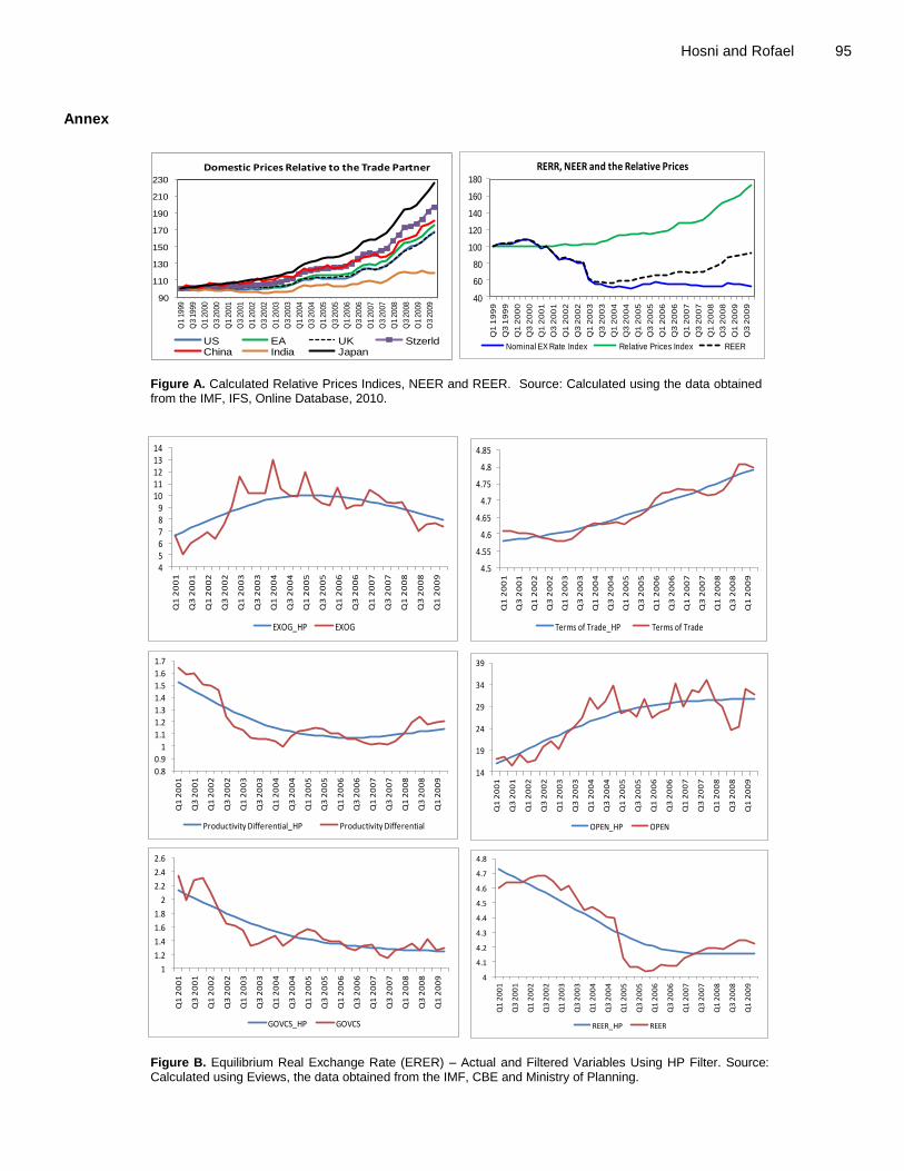
4For further clarification of that point, refer to the relative prices index graphs in the annex.

84 J. Econ. Int. Finance because starting from April 1999; the CBE carried out a series of devaluations in the Egyptian Pound, which resulted in the dramatic increases in the relative prices due to the pass-through effect.

This section is divided into two main parts. The first part tackles the observed Real Effective Exchange Rate (REER) calculations. While the second part, the Equilibrium RER and the misalignments are estimated. Observed real effective exchange rate (REER) The paper starts by getting the weights for Egypt’s main trading partners. For simplicity reasons, authors included the partners whose average trade share with Egypt covers about 70% of its total trade with the world in 2007-2008 and 2008-2009 (CBE, 2010). The formula that the paper relied upon for calculating the REER is given by equation (1). In the context of calculating the REER, the summation of the trade share should add up to one, so it is suggested to adopt a standardization technique to adjust the shares as illustrated in Table 1.

100**

W

P

P

e

eREER

i

fi

dt

io

it

ijt

(1) Where eit = foreign exchange rate of country (i) in terms of the domestic currency in the period (t); ei0 = foreign exchange rate of country (i) in terms of the domestic currency in the period (0); Pdt = domestic inflation rate in the period (t); Pfi = trade partner country (i)'s inflation rate in the period (t); Wi = the trade share of the partner country (i) in the total trade of a particular country (j). Moreover, to calculate the REER, CPI (1999=100) and nominal domestic exchange rates of all the trading partners versus the US dollar were gathered for the period Q1:1999 to Q2:2009. Worth mentioning, the exchange rate for the trade partners in terms of the US dollar represents the period average. However, the exchange rate used for Egypt's case is the end of period.5 For further information about the price indices and the calculated observed REER, refer to Figure A in the annex.

Equilibrium Real Exchange Rate (ERER) and Misalignments

The current section presents three different methodological approaches in estimating the equilibrium RER by applying the PPP approach, Edwards' model and the FEER approach (known as the External Sustainability Approach), in the framework of the model-based approach.

Purchasing power parity approach

In estimating the equilibrium RER in the context of the PPP

approach, the paper assumes that the ERER is the average of the observed REER over a 10-years period. That average acts as a benchmark through which the misalignments could be detected. This implies that whenever the observed REER overshoots the average, the Egyptian Pound experiences overvaluation. However, when the observed REER moves beneath the benchmark, the Egyptian Pound is undervalued. Although this technique is widely

5Source of data IFS – IMF, online database accessed in June 2010.

criticized because it lacks the dynamics taking place in the productivity in the tradable sector compared to the non-tradable sector, the paper insisted on its calculation to get preliminary insights about the real exchange rate misalignments before digging deeply by applying the model-based approaches. Fundamental equilibrium exchange rate (FEER) approach or external sustainability The FEER concept is based on the notion of macroeconomic balance, which has both internal and external dimensions. The core idea of the macroeconomic balance approach is the Balance of Payments (BOP) identity, which equates the current account to the negative capital account. As such, the exchange rate that is consistent with the macroeconomic balance (the FEER) is the real effective exchange rate that will bring the current account into equality with the sustainable current account where the determinants of the current account have been set at their full employment values (Clark and Macdonald, 1998).

On the other hand, the IMF consultative group of exchange rate assessment defined the FEER as the External Sustainability approach, which involves estimating the adjustment in the REER needed to stabilize the NFA to the GDP ratio at a certain benchmark level. This approach focuses on the relation between the sustainability of a country’s external stock position and its flow current account position and the real exchange rate. It relies on an inter-temporal budget constraint, which requires that the present value of future trade surpluses is sufficient to pay for the country’s outstanding external liabilities. One of the simple ways to satisfy a country’s inter-temporal budget constraint is to ensure that the size of the net foreign assets is stabilized relative to the size of the economy (a stable NFA/GDP ratio), thus preventing assets or liabilities from growing without bound.

Applying this approach consists of three steps:

1. Determining the current account balance to GDP ratio that would stabilize the NFA position at a given “benchmark” value. 2. Comparing this NFA-stabilizing current account balance with the level of a country’s current account balance expected to prevail over the medium term. 3. Assessing the adjustment in the real effective exchange rate over the medium term that would bring the current account balance in line with its NFA-stabilizing level.

Worth mentioning, the ES approach requires only a few assumptions about the economy, including: the potential real GDP growth rate that will prevail in the medium term; an average inflation profile; and setting a level at which external indebtedness should be satisfied (external indebtedness is defined as the NFA position, and the benchmark level is its latest observed value). This approach implies that economies that grow faster can afford to run larger current account deficits and smaller trade balances without increasing their ratio of external liabilities to GDP.

To determine the level of the current account balance that stabilizes NFA at a given level, we use the BOP accounting identity that holds at all times, which is:

0

&)(

OmissionsErrorsNet

t

accountfinancialAssetsinTrade

AtLt

AccountCapital

t

AccountCurrent

t ZHHKCA

(2)

The paper then derives the equation, which states that the changes in net foreign assets are due to either the net financial flows (net purchases of foreign assets minus net foreign purchases of domestic assets) or the changes in the valuation of outstanding foreign assets and liabilities:

gainscapitalincludingFlows

tttt

NFAinChanges

tt ZKGKCABB 1

(3) Where Bt is the net foreign assets, CAt is the current account balance, Kt are capital transfers, KGt are capital gains arising from valuation changes, and Zt are errors and omissions that can drive a wedge between the current account balance and the net financial flows.

Assuming that Kt, KGt, and Zt are zero, dividing equation (2) by

nominal GDP growth rate t , and then denoting the ratios to GDP by lower case letters, the equation will be:

t

t

t

ttt cabbb

111

(4) Then the current account level (denoted by cas) that stabilizes the net foreign assets at a benchmark level (denoted by bs) is:

ss b

g

gca

11 (5)

Where gt is the real GDP growth rate and πt is the inflation rate. Equation (4) implies the following links between the current account, the economic growth, inflation, and the net external position:

1. The current account balance consistent with stabilizing the ratio of net foreign assets to GDP at level bs is proportional to bs (moving in the same direction). For example, for a country with a nominal growth rate of 7 percent, the current account balance necessary to stabilize the net foreign assets at -50 percent of GDP is about -3.5 percent. However, for the same level of nominal growth, the current account balance will be -2.8 percent that would able to stabilize the net foreign assets at -40 percent of GDP. 2. The absolute size of the current account balance consistent with stabilizing net foreign assets at any given level bs is proportional to the rate of growth. So the current account balance consistent with stabilizing the net foreign assets at -50 percent of GDP becomes -2.5 percent of GDP if the nominal growth rate is 5 percent, compared to the value of -3.5 percent when growth rate was assumed to be 7 percent, in the previous example. Equilibrium real exchange rate based on Edward’s Model (1989)

An important motivation for estimating the ERER is to quantify the magnitude of RER misalignments during the study period spanning from 2001: Q3 to 2009: Q4.6 In this context, the paper follows Edwards' model (1989) based on a Vector Error-Correction Model (VECM) to estimate the long-term path of the RER as a function of a group of economic fundamentals. Accordingly, stationarity test based on Augmented Dickey Fuller (ADF) test is carried out to examine the degree of integration among the incorporated variables.

6For the sake of consistency check, Edwards’ model will be re-estimated using

a different data sample with annual frequency that spans from 1974 through

2012. This helps to draw robust stylized fact about exchange rate dynamics in Egypt.

Hosni and Rofael 85

Turning to the incorporated variables and the data sources, the analysis utilizes the data for the GDP, government expenditure, exports, imports, current account inflows, the price indices and the nominal exchange rates. All the data is gathered from the International Financial Statistics database (IMF), Central Bank of Egypt and the Ministry of Planning. Practically, the paper relies on a particular group of economic fundamentals upon which the empirical literature has a consensus, especially for the developing countries. As such, the relative per capita GDP is a proxy for the productivity differential. It is calculated as the ratio between the Egyptian per capita income relative to the per capita income of the three main trading partners; the Euro area, USA and the UK, weighted by their trade shares. The terms of trade variable are proxied by the Egyptian Consumer Price Index (CPI) relative to the Producer Price Indices (PPI) for the above mentioned three partners. A variable for the degree of openness is included and it is calculated as the ratio between the total trade to GDP. Moreover, the government consumption as a ratio of GDP and the exogenous current account receipts as a ratio of GDP are incorporated. The exogenous receipts include the revenues obtained from the Suez Canal and the tourism sector (see Figure (B) in annex). Finally, two exogenous dummy variables are suggested in the sense that one can account for the exchange rate floatation in 2003, whereas the second one accounts for the Global Financial Crisis, which took place in 2008.

Methodologically, the ERER estimation is conducted through two main steps. First, the long run coefficients are obtained from a reduced-form equation based on Johansen co-integration test as in equation (6) and a Vector Error Correction Model (VECM), with two exogenous dummies (Tables 9 and 10 in annex). The lag length is determined based on Akaike information criterion, showing two lags in levels and one lag in difference. In this context, the included variables are introduced to the estimation process without any adjustments (i.e. transitory and the permanent components are maintained). Afterwards, the estimated long run coefficients for all variables are used to calculate the ERER after filtering the original variables by excluding the transitory components; using a smoothing technique; the paper relies on Hodrick-Prescott (HP) Filter. Noteworthy, if no co-integrating relationship is found, then this implies that the incorporated fundamentals are not the appropriate variables that capture the long-run ERER, thus in this case variables revision is recommended until the co-integrating relationship is obtained.

ttt

p

iitt XYYY

1

1

11

(6)

Where:

Y t: vector of non-stationary I(1) variables

: refers to a reduced form matrix equals (α β'), where (α) is the adjustment parameter in the vector error correction model and (β) is the co-integrating vector

X t : is the vector of the deterministic (exogenous) variables

t : is the vector of innovations

i : Short-run dynamics estimates

It is noteworthy that the theme of the analysis stems mainly from the relationship between the tradable and non-tradable sectors. In addition, the expected signs of most of the estimated coefficients are settled upon in the empirical literature (refer to equation (7)).

The coefficients (β4) and (β6) are expected to have positive signs; because any improvement in any of these variables will stimulate the demand on the non-tradable goods, resulting in higher domestic

86 J. Econ. Int. Finance prices and consequently real appreciation. Intrinsically, the impact of (β6) is known as Balassa-Samuelson effect, because the improvement in the productivity of the tradable sector will cause the increase in the wages of those employed in that sector; inducing higher wages in the non-tradable sector. If this is not accompanied with a higher productivity in the non-tradable sector, then an increase in the overall price level will result and consequently real appreciation. Similarly, the impact of (β4) is very intuitive, in the sense that any increase in the current account inflows would increase the country's disposable income, consequently higher price level and real appreciation. This mechanism is called the Dutch Disease effect (IMF, 2007). On the contrary, coefficient (β2) is expected to have a negative sign, implying that the higher the degree of openness, the higher the degree of real depreciation because spending will be diverted to the tradable goods. Δ (LREER) = α [β1LREERt-1 + β2OPENt-1 + β3LTOTt-1 + β4EXOGt-1 + β5GOVCSt-1 + β6GDPDt-1 + β0] + [τ1 Δ (LREERt-1) + τ2 Δ (OPENt-1) + τ3 Δ (LTOTt-1) + τ4 Δ (EXOGt-1) + τ5 Δ (GOVCSt-1) + τ6 Δ (LGDPDt-1)] + λ1DUMEX + λ2DUMCRIS + C (7) Where: LREER: logarithm of the observed real effective exchange rate OPEN: refers to the degree of openness, sum of total trade relative to GDP LTOT: logarithm of the terms of trade EXOG: exogenous current account inflows of the Suez Canal receipts and tourism receipts GOVCS: government expenditure to GDP ratio LGDPD: logarithm of the Egypt's GDP per capita relative to that of the main trading partners DUMEX: dummy variable for the shift of exchange rate regime from fixed to float in 2003 DUMCRIS: dummy variable for the incidence of the global financial crisis in 2008 Nevertheless, the signs of (β3) and (β5) are undecided because they might have positive or negative signs. As for the sign of the government coefficient (β3), the issue depends on whether the increase in the government consumption is directed to the tradable (equivalent to real depreciation) or to the non-tradable goods (equivalent to real appreciation). Turning to the expected sign of the terms of trade (β5), it has been argued that the idea depends on which effect is stronger, whether the income or the substitution effect. Implicitly, if the terms of trade improve (Price exports > Price imports), then the disposable income rises, thus the two effects are demonstrated. The substitution effect will induce the producers to direct the available resources to produce the tradable products leading to higher supply of tradables relative to non-tradables, thus higher non-tradable prices and real appreciation. On the contrary, the income effect will induce the producers to maintain the same level of income even if they reduce the supply of tradables, thus higher prices of tradables that leads to real depreciation. The opposite will happen if the terms of trade deteriorated.

Once the equilibrium RER is calculated, the RER misalignment could be easily obtained as the difference between the observed RER and the equilibrium RER. According to the model structure used, any positive (negative) values mean overvaluation (undervaluation) in the Egyptian Pound. RESULTS

This section presents the outcomes of the three aforementioned techniques used to estimate the RER misalignments in the Egyptian Pound. The rest of the

section is organized as follows: first, displaying the PPP results followed by the findings of the accounting external sustainability approach. Finally, the section ends up with the empirical evidence captured from the econometric model based on Edwards (1989). Purchasing Power Parity Approach As per this approach the ERER is calculated as the 10-years average rate for the period 1999-2009 that is found to be 79.7. This is calculated to get a preliminary insight about the real misalignment before the paper digs deeply by applying the ES approach and Edwards’s model. It is noticed that the Egyptian Pound was over-valued during the period (1999:Q1 to 2002:Q4) since the actual REER exceeded the Average Equilibrium REER of 10 years (Figure 1). This reached an end by the steps of devaluation that the CBE had taken over the mentioned period; then the Egyptian pound registered the trough rate after announcing the official floatation of the Egyptian Pound.

Nevertheless, during the above-mentioned period, the actual REER had a downward trend; implying real depreciation that was supported by the steps of the devaluation on one hand, and the inflation differential in favor of the Egyptian economy on the other hand.

The second period extends from 2003:Q1 to 2008:Q2, wherein the Egyptian pound was under-valued. During this period, the REER experienced two different patterns; the first was real depreciation that was due to the nominal depreciation resulting from the floatation announcement at 2003 till 2004:Q4. Since then, the Pound started to appreciate due to the nominal appreciation of the Pound and the deterioration of inflation differentials in favor of the main trading partners over the following three years till 2008:Q2 (refer to Figure A in the annex).

Over the third period (2008:Q2 to 2009:Q4), the Pound started to be over-valued once again, a situation that can be attributed to the increasing levels of the domestic price level that exceeded the international prices; due to the economic slowdown that our partners faced during the second half of 2008 because of the Global Financial Crisis. This was reflected as well in a real appreciation that would adversely affect the Egyptian economy's competitiveness in the international markets.

Fundamental Equilibrium Exchange Rate (FEER) Approach For the sake of calculating the ERER in Egypt by relying on the external sustainability approach, the study had to go through three main steps as follows: first, choosing the benchmark level for NFA (as a ratio of GDP), using the CBE International Investment position (IIP) data in 2009 that was found to be - 14.0%. Second, calculating the Current Account (CA) balance (as a ratio of GDP) that

Hosni and Rofael 87

Figure 1. The development of the REER based on the PPP approach (1999: Q1=100). Source: IMF, IFS, Online Database, November 2010 and CBE, monthly bulletin.

Table 1. Egypt’s main trading partners (average 2007/2008 and 2008/2009).

Standardized share Trade share

37 26 Euro Area (16)

30 21 USA

10 7 UK

8 5 Switzerland

6 4 China

5 3.4 India

4 2.6 Japan

100 69 Total

Source: CBE Monthly Bulletin, Various Issues.

would stabilize the NFA at the benchmark level for four consecutive years (2011-2014) using equation (5) displayed in the previous section. In this context, the study utilizes the World Economic Outlook (WEO) medium-term projections of the inflation rate and the potential Real GDP growth rate that would prevail in each of these years.

7 Against this background, CA balances

that would stabilize NFA/GDP ratio at the benchmark level are computed (these balances represent equilibrium CA and implicitly indicate the equilibrium REER level).

Finally, the authors compare the gap between the projected current account that would prevail in the projec- ted years, and the current account stabilizing NFA; it has been found that Egypt's REER will be over-valued during

7WEO projections for percent change in prices (Π) are 9.5%, 8.5%, 7.8%, and

7.0%; and real GDP growth rate (g) are 5.5%, 5.7%, 5.9%, and 6.2% for 2011 till 2014, respectively.

Table 2. Equilibrium Real Effective Exchange Rate (EREER) applying External Sustainability (ES) approach.

2014 2013 2012 2011

-14.01 NFA Benchmark 2009 (%of GDP)

-1.63 -1.65 -1.74 -1.83 CA-Balance Stabilizes NFA (%of GDP)

-1.64 -1.71 -2.02 -2.10 Projected CA Balance (%of GDP)

0.22 1.91 9.15 9.13

Misalignment

(+) Overvaluation

(-) Undervaluation

the four years as shown in Table 2. It is noteworthy that in order to quantify the percentage change in REER needed to fill the gap between the projected current account balance and the current account level at the NFA- stabilizing benchmark level; the paper employed a simple regression between the REER and the current account balance (as a ratio of GDP) for the period 1999–2009. The elasticity computed from this regression states that 1 percent depreciation (appreciation) in the REER, leads to 0.03 percent improvement (deterioration) in the CA balance (as a ratio of GDP).

To sum up the main findings of the ES approach, it is concluded that in order to correct REER misalignments, some policy actions should be taken to restore the equilibrium level by stabilizing the Egyptian economy's NFA (as a ratio of GDP) at its benchmark level in a selected year from 2011 to 2014. Practically, the issue depends on the policy maker's preferences. Evidently, it

50

60

70

80

90

100

110

120

Q1 1

999

Q3 1

999

Q1 2

000

Q3 2

000

Q1 2

001

Q3 2

001

Q1 2

002

Q3 2

002

Q1 2

003

Q3 2

003

Q1 2

004

Q3 2

004

Q1 2

005

Q3 2

005

Q1 2

006

Q3 2

006

Q1 2

007

Q3 2

007

Q1 2

008

Q3 2

008

Q1 2

009

Q3 2

009

Chart (1): The Development of the REER based on the PPP approach(1999:Q1=100)

NEER REER Average-10 Years

88 J. Econ. Int. Finance is suggested that the magnitude of real depreciation is determined based on one of two scenarios: either the policy maker chooses to reach equilibrium in 2011 or 2012; in this case, the REER has to be depreciated by 9.1 or 9.2%, respectively from 2009 level. Or, the policy maker decides to reach equilibrium in 2013 or 2014, which showed a different pattern; in this case, the REER has to be depreciated by 1.9 or 0.2%, which is an insignificant rate of depreciation, for example: maintain 2009 REER level.

Equilibrium Real Exchange Rate based on Edwards Model (1989)

The application starts by testing the order of integration of each variable based on Augmented Dickey Fuller (ADF) unit root test. The result shows that all the incorporated variables are integrated of the first order (i.e. I (1) (Table 3). This suggests that it is more likely to find a co-integrating relationship among these variables.

Moreover, the Johansen co-integration test is employed wherein both the Trace Statistics and the Maximum Eigen Value indicate the existence of three co-integrating equations at 95% and 99% confidence levels among the selected variables; implying the stability of the equilibrium relationship. Since the restrictions on the estimated parameters (β) should be captured from the economic theory yet, the theory did not tackle that issue. In addition, estimating more than one co-integrating vector will complicate the economic interpretation of the long-run relationship between the REER and the economic fundamentals. Therefore, the paper relied on the long run estimates of one co-integrating equation without imposing any restrictions to estimate the three co-integrating equations. The long run estimated coefficients appear to be consistent with the economic theory concerning their signs, except the productivity differential estimate that is statistically insignificant and carries a wrong sign. This is so intuitive and implies that Balassa-Samuelson mecha- nism is not suitable for the Egyptian case. In fact, the whole issue deals with the relative wages and productivity between the tradable and the non-tradable sectors, whereas these relationships suffer significant distortions in Egypt due to labor market rigidities.

The estimated long run equilibrium and short run dynamics estimates are given by equation (8). The error correction term (α) appears negative and significant implying that equilibrium is restored back when there exists a misalignment between the observed REER and the ERER. The adjustment term is equal to 9.2% per quarter. This indicates that it takes from 2.5 to 3 years for the real exchange rate to restore back its equilibrium level. Δ (LREER) = -0.092 [LREERt-1 + 0.010 OPENt-1 - 5.358 LTOTt-1 - 0.360 EXOGt-1 - 1.210 GOVCSt-1 - 1.675 LGDPDt-1 + 21.175] + [0.224 Δ (LREERt-1) + 0.002 Δ

Table 3. Augmented Dickey Fuller Unit Root Test Results.

First difference Level

-3.25 -1.33 LREER

-2.69 -2.56 LGDPD

-3.37 -0.69 LTOT

-4.39 -1.70 GOVCS

-4.77 -2.32 EXOG

-4.30 -1.58 OPEN

Note: the displayed results are employed using ADF test with intercept and 1 lagged difference. The critical values at level are -2.956 and -2.616 at 5% and 10%, respectively. While the critical values at first difference are -2.959 and -2.618 at 5% and 10%, respectively. Source: Authors’ estimations using EViews software. (OPENt-1) - 0.017 Δ (LTOTt-1) - 0.013 Δ (EXOGt-1) – 0.043 Δ (GOVCSt-1) + 0.150 Δ (LGDPDt-1)] – 0.103 DUMEX + 0.0521 DUMCRIS + 0.063 (8) Additionally, to estimate the EREER and then get a measure for the RER misalignment, the literature suggests a smoothing technique to exclude the transitory effects embedded in the economic fundamentals as long as the ERER is a long-run phenomenon. In this context, HP filter is utilized to capture the persistent component in each variable (see Figure (B) in annex). Subsequently, the estimated long run coefficients are applied to the new time series. The results, as illustrated in Figure 2, show that the Egyptian RER experienced two overvaluation episodes: the first was spanning from 2001 till the announcement of the exchange rate flotation in 2003; whereas the second episode of overvaluation was experienced in 2008 and 2009. On the other hand, during the period between 2003 and 2008, the RER witnessed substantial undervaluation that was fortunately accom-panied by favorable current account balances. Interestingly, these findings came in line with previous conclusions obtained by Riad (2008).

An interesting finding is that these results are in line with the early findings presented in the PPP approach. The two methods coincide in the periods of undervalue-tion and overvaluation despite the fact that each of them reveals different misalignment magnitude. For example, in 2009, the estimations based on Edwards' model suggest that the RER is misaligned on average by 6.6% from its equilibrium level. However, although the PPP approach indicates overvaluation as well, yet with diffe-rent magnitude equals to 13% from its equilibrium level.

Equilibrium Real Exchange Rate based on Edwards Model (1989): An extension In this section, the paper presents the re-estimation of Edwards’s model using annual data set, which portrays the relationship between equilibrium real exchange rate

Hosni and Rofael 89

Figure 2. Observed REER, equilibrium and misalignments based on Edwards' Model estimation, overvaluation and undervaluation.

and a set of five economic fundamentals expressed as a vector of the following variables

8:

Xt = (LREER, LGDPC, OPENGDP, INVESTGDP, LGOVCONS) (9) It is worth to mention that although the previous section presented the same methodology while using higher frequency data, the sample was too small to draw conclusions about the exchange rate misalignment or to provide adequate policy implications. Given such data limitations and statistical implications, it was found more convenient to update the estimations through re-running the model while covering a larger time span that ranges between 1974 and 2012.

A necessary condition of the co-integration and VECM analysis is that each of the variables should be stationary and integrated of same order. Hence, the first step of our empirical work is to check the degree of integration of each variable by using unit root test (ADF and PP) for the levels and first differences of each variable. The estimated results of this part are reported in Table 4.

It was found that each of the series is non-stationary when the variables are defined in levels. But first-

8The study makes use of annual data as early mentioned. Data availability constrains the sample period to 1974 to 2012. Definitions of the five

endogenous variables and two exogenous variables along with their sources are

as follows: LREER: logarithm of REER, constructed by the authors using data from the IMF, IFS and IMF, DOTS databases. LGDPC: logarithm of per capita

GDP as a proxy for relative productivity differential between Egypt and its

trading partners, obtained from the World Bank (WB), WDI database. OPENGDP: Exports and Imports as a ratio of GDP, data obtained from the

IMF, DOTS and WB, WDI database. INVESTGDP: Investment ratio to GDP,

data obtained from the WB, WDI database. LGOVCONS: logarithm of government consumption, obtained from the WB, WDI database.

FLOATDUM: a dummy for the float of the Egyptian pound that takes a value

of one starting from 2003. CRISDUM: a dummy for the global financial crisis that takes a value of one starting from 2008.

differencing the series removes the non-stationary components in all cases and therefore, the null hypothesis of non-stationarity is clearly rejected at the 5 percent significance levels. Both the ADF and PP stationarity tests suggest that all the variables are integrated of order one (I (1)) in their levels and found stationary in their first differences (I (0)).

Since the variables are stationary and integrated of order one, this paved the way to applying a co-integration technique to test whether there exist a long-run relationship among the variables. In this context, Johansen (1988) provided a unified framework for estimation and testing of co-integrating relations in the context of a VAR error correction model. The co-integration rank (r) of the time series was tested using our two test statistics; λtrace and λmax. Denoting the

number of co-integrating vectors by , the maximum eigenvalue (λmax) test is calculated under the null

hypothesis = r against an alternative hypothesis = (r + 1). The trace test (λtrace) is calculated under the null

hypothesis that ≤ r against > r. The results of both statistics are reported in Table 5.

The results of the co-integration show that both the trace and the maximum eigenvalue test statistics suggest the existence of only one co-integrating relationship among our variables at both the 1 percent significance level. This gives an evidence for a long-run equilibrium relationship between the real effective exchange rate in Egypt, GDP per capita denoting the productivity differential between Egypt and its main trading partners, investment as a share of GDP, openness of the Egyptian economy, and government consumption.

To determine the sign and magnitude of the long run relationship, the co-integrating vectors were normalized so that the co-integrating regression of the REER in

-15

-10

-5

0

5

10

15Q

1 2

00

1

Q3

20

01

Q1

20

02

Q3

20

02

Q1

20

03

Q3

20

03

Q1

20

04

Q3

20

04

Q1

20

05

Q3

20

05

Q1

20

06

Q3

20

06

Q1

20

07

Q3

20

07

Q1

20

08

Q3

20

08

Q1

20

09

Real Exchange Rate Misalignment (%)

3.803.904.004.104.204.304.404.504.604.704.80

Q1

20

01

Q3

20

01

Q1

20

02

Q3

20

02

Q1

20

03

Q3

20

03

Q1

20

04

Q3

20

04

Q1

20

05

Q3

20

05

Q1

20

06

Q3

20

06

Q1

20

07

Q3

20

07

Q1

20

08

Q3

20

08

Q1

20

09

Observed REER and Equilibrium RER

Observed REER Equil REER

Overvaluation

Undervaluation

Overvaluation

90 J. Econ. Int. Finance

Table 4. Unit root tests results

Augmented Dickey-Fuller (ADF) Test Phillips-Perron (PP) Test

Levels Variables Model Form: Intercept Model Form: Intercept

LREER -3.49 -2.45

LGDPC -0.81 -0.77

OPENGDP -0.64 -0.72

INVESTGDP -1.70 -2.27

LGOVCONS -2.44 -1.65

First Differences Variables Model Form: Intercept Model Form: Intercept

LREER -4.24* -3.79*

LGDPC -3.59* -4.89*

OPENGDP -4.48* -6.43*

INVESTGDP -5.26* -10.18*

LGOVCONS -4.63* -6.67*

*Denotes significance at the 5 percent level and the rejection of the null hypothesis of non-stationarity. Mackinnon (1991) critical values for rejection of hypothesis of unit root are applied. The critical values at 5 percent significance level are -3.5348 and -3.5312 for ADF and PP tests, respectively. Source: Authors’ estimations using EViews software.

Table 5. Johansen’s co-integration likelihood ratio test for multiple co-integrating vectors.

Trace Statistic Maximum Eigenvalue Statistic

Ho HA λtrace CV1% Ho HA λmax CV1%

r0 = 0 r1 > 0 108.60* 76.07 r0 = 0 r1 = 1 58.07* 38.77

r0 ≤ 1 r1 > 1 50.53 54.46 r0 = 1 r1 = 2 27.86 32.24

r0 ≤ 2 r1 > 2 22.66 35.65 r0 = 2 r1 = 3 13.70 25.52

r0 ≤ 3 r1 > 3 8.96 20.04 r0 = 3 r1 = 4 6.14 18.63

r0 ≤ 4 r1 > 4 2.82 6.65 r0 = 4 r1 = 5 2.82 6.65

N.B: i. (r) refers to number of co-integrating equations.ii. CV1% refers to the critical value at the 1 percent significance level. * Denotes rejection of the hypothesis at the 1 percent level. Source: Authors’ estimations using EViews software.

Egypt can be given as shown in Table 6. The long run estimated coefficients appear to be

consistent with the economic theory concerning their expected signs. It appears that the productivity differential cause an appreciation of the real effective exchange rate in Egypt. The effect of the openness of the economy is dominated by substitution effects

9 since it leads to a

depreciation of the real effective exchange rate as well. Regarding the investment ratio, it has a depreciating effect on the real effective exchange rate in Egypt. This can be explained by the import intensive investment projects and thus; an increase in the ratio of investment to GDP is expected to increase absorption, worsen the current account and lead to depreciation of the REER. Government consumption causes an appreciation of the

9 Substitution effect stems from the fact that trade liberalization reduces the

domestic prices of tradables causing a demand shift away from non-traded

goods. It is argued that given reasonable cross-price elasticities, non-traded prices should go down leading to a real depreciation.

REER, since this gives a clue about the structure of the government expenditure that gives higher weight to the non-tradables compared to the tradables. As such, higher government expenditure would be mirrored in higher demand on non-tradable goods and services, which in turn would raise the prices of non-tradables (Table 6).

The results suggest the following magnitude of effects:

- A 1 percentage point increase in the differential between the rate of growth of the real per capita GDP in Egypt and its main trading partners is associated with a 0.85 percentage point appreciation of the REER in the long run.

- A 1 percentage point increase in the relative openness of the Egyptian economy is associated with a 0.60 percentage point depreciation of the REER in the long run.

- A 1 percentage point increase in the relative investment

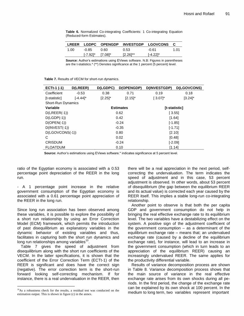
Hosni and Rofael 91

Table 6. Normalized Co-integrating Coefficients: 1 Co-integrating Equation (Reduced-form Estimates).

LREER LGDPC OPENGDP INVESTGDP LGOVCONS C

1.00 -0.85 0.60 0.53 -0.61 1.01

[-7.92]* [7.08]* [2.26]** [-4.22]*

Source: Author’s estimations using EViews software. N.B: Figures in parentheses are the t-statistics.* (**) Denotes significance at the 1 percent (5 percent) level.

Table 7. Results of VECM for short-run dynamics.

ECTt-1 (-1) D(LREER) D(LGDPC) D(OPENGDP) D(INVESTGDP) D(LGOVCONS)

Coefficient

[t-statistic]

-0.53

[-4.44]*

0.38

[2.25]*

0.71

[2.15]*

0.19

[ 3.07]*

0.18

[3.24]*

Short-Run Dynamics

Variable Estimates [t-statistic]

D(LREER(-1)) 0.62 [ 3.55]

D(LGDP(-1)) 0.42 [1.64]

D(OPEN(-1)) -0.24 [-1.85]

D(INVEST(-1)) -0.35 [-1.71]

D(LGOVCONS(-1)) 0.80 [2.10]

C 0.02 [0.48]

CRISDUM -0.24 [-2.09]

FLOATDUM 0.10 [1.14]

Source: Author’s estimations using EViews software.* indicates significance at 5 percent level.

ratio of the Egyptian economy is associated with a 0.53 percentage point depreciation of the REER in the long run. - A 1 percentage point increase in the relative government consumption of the Egyptian economy is associated with a 0.61 percentage point appreciation of the REER in the long run. Since long run association has been observed among these variables, it is possible to explore the possibility of a short run relationship by using an Error Correction Model (ECM) framework, which permits the introduction of past disequilibrium as explanatory variables in the dynamic behavior of existing variables and thus, facilitates in capturing both the short run dynamics and long run relationships among variables

10.

Table 7 gives the speed of adjustment from disequilibrium along with the short run coefficients of the VECM. In the latter specifications, it is shown that the coefficient of the Error Correction Term (ECTt-1) of the REER is significant and does have the correct sign (negative). The error correction term is the short-run forward looking self-correcting mechanism. If for instance, there is a real undervaluation in the REER, then

10As a robustness check for the results, a residual test was conducted on the estimation output. This is shown in figure (c) in the annex.

there will be a real appreciation in the next period, self-correcting the undervaluation. The term indicates the speed of adjustment and in this case, 53 percent adjustment is observed. In other words, about 53 percent of disequilibrium (the gap between the equilibrium REER and its actual value) is corrected each year caused by the REER itself. This implies a stable long-run co-integrating relationship.

Another point to observe is that both the per capita GDP and government consumption do not help in bringing the real effective exchange rate to its equilibrium level. The two variables have a destabilizing effect on the system. A positive sign of the adjustment coefficient of the government consumption – as a determinant of the equilibrium exchange rate – means that; an undervalued exchange rate (caused by a decline of the equilibrium exchange rate), for instance, will lead to an increase in the government consumption (which in turn leads to an appreciation of the equilibrium REER) causing an increasingly undervalued REER. The same applies for the productivity differential variable.

Results of variance decomposition process are shown in Table 8. Variance decomposition process shows that the main source of variance in the real effective exchange rate arises from its own shocks during all pe-riods. In the first period, the change of the exchange rate can be explained by its own shock at 100 percent. In the medium to long term, two variables represent important

92 J. Econ. Int. Finance

Table 8. Results of variance decomposition analysis.

Period S.E. LREER LGDPC OPENGDP INVESTGDP LGOVCONS

1 0.15 100.00 0.00 0.00 0.00 0.00

2 0.24 97.00 0.10 1.07 0.59 1.24

3 0.29 90.02 0.73 6.86 1.52 0.87

4 0.33 74.13 0.75 15.68 7.34 2.10

5 0.38 58.04 0.57 22.55 13.78 5.06

6 0.43 46.74 0.46 26.95 18.15 7.69

7 0.47 39.06 0.39 30.00 21.03 9.52

8 0.52 33.42 0.34 32.25 23.15 10.84

9 0.56 29.03 0.30 33.94 24.84 11.90

10 0.60 25.57 0.27 35.21 26.18 12.77

Source: Author’s estimations using EViews software.

sources of variation in the exchange rate. These are the openness and investment ratios. For example and starting from the third period, it is seen that economic openness explains the variation in real effective exchange rate at a rate that ranges between nearly 7 percent and 35 percent. Between 1.5 and 26 percent of the variation in the exchange rate can be explained by the investment ratio. Government consumption plays a more significant role in the variations of the real effective exchange rate from the fourth period onwards while productivity differential do not exceed the rate of 0.8 percent variation of exchange rate during all periods.

An important feature of Edwards’ approach is the recognition that the equilibrium exchange rate change over time with the changes in its main fundamentals. The long-run relationship estimated above allows for the calculation of the equilibrium rate by imposing the long-run coefficients of the economic fundamentals employed to the permanent values of the latter. The HP filter with a smoothing factor of 100 was used to smooth the variables

11. Figures 3 and 4 show the actual and

equilibrium real effective exchange rate and the extent of currency misalignments during the period (1974-2012) (Table 8).

When the actual real effective exchange rate is above the equilibrium, it is undervalued, and when it is below the equilibrium, it overvalued. Through 1974 up till 1990, before the implementation of the ERSAP, the Egyptian trade-weighted exchange rate was always overvalued with the exception of the period (1979-1982). Starting from 1991, Egypt witnessed an undervaluation of the exchange rate that continued till 1998. This means that the unification of the multiple exchange rates that existed before the ERSAP brought a temporary end to the currency overvaluation.

Thus, despite the real appreciation of the Egyptian pound during that period, it was not as much as is

11This smoothing factor is what Hodrick and Prescott suggested for annual data (EViews User’s Guide).

Figure 3. Actual and equilibrium real effective exchange Rate in Egypt based on Edwards’ approach during 1974-2012 - in logs. Source: Author’s estimations using EViews software.

Figure 4. Misalignments of the Actual Real Effective Exchange Rate in Egypt Based on Edwards’ Approach during 1974-2012 - in percent. Source: Author’s estimations using EViews software.

0.2

0.21

0.22

0.23

0.24

0.25

0.26

0.27

197

4

197

6

197

8

198

0

198

2

198

4

198

6

198

8

199

0

199

2

199

4

199

6

199

8

200

0

200

2

200

4

200

6

200

8

201

0

201

2

Observed REER Equilibrium REER

-3

-2

-1

0

1

2

3

4

197

4

197

6

197

8

198

0

198

2

198

4

198

6

198

8

199

0

199

2

199

4

199

6

199

8

200

0

200

2

200

4

200

6

200

8

201

0

201

2

▲Overvaluation

▼ Undervaluation

needed to keep the value of the pound in line with the calculated average equilibrium rate in real terms, a conclusion that can be reasonably thought of under the improved economic conditions that accompanied the beginning of the economic reform in Egypt. In addition, this is suggestive of the active and periodical foreign exchange market intervention that was practiced during that period to maintain the pegged exchange rate – mainly through the international reserves – and thus, preventing the free market determination of the pound’s value. Mohieldin and Kouchouk (2003) describe the first half of the 1990s decade by an undervalued currency based on the latter’s own calculations as well.

A short overvaluation period during the three years between 1999 and 2001 was followed by an under-valuation period that lasted between 2002 and 2008. The latter period marked the consequences of the series of devaluations adopted in 2000 and 2001 and the floatation of the Egyptian pound in 2003. Overvaluation of the Egyptian real effective exchange rate was resumed in 2009 and lasted till the end of the sample employed in the present study. This came just in line with the early misalignment findings in the previous section. Impor-tantly, it also conforms to the judgment of the IMF’s 2010 Article IV consultation report on the Egyptian economy.

CONCLUSION AND POLICY RECOMMENDATIONS The paper acquires its importance from the fact that the exchange rate misalignment or the permanent deviation of the actual exchange rate from its equilibrium level could have adverse impact on the macroeconomic stability. Thus, the exchange rate misalignment would be of a great interest to the policy makers in general and to the monetary authority and Central Banks in particular. Since the exchange rate is considered an important monetary transmission mechanism channel that could affect both the economic activity and the economy-wide price level. Therefore, real effective exchange rate move-ments can directly affect consumption and production choices between domestic and international goods. Tracing those movements would help the policy makers in avoiding economic instability created from the distor-tions resulted in the relative prices between the tradable and non-tradable goods due to keeping the exchange rate away from its equilibrium level for a long time.

Against this background, the paper tries to adequately assess the real exchange rate in Egypt during the period 1999-2009, based on three different methodologies that both theoretical and empirical literature has focused upon. The carried out techniques are the PPP approach, the FEER approach and Edwards’s model that was introduced in 1989. Fortunately, the three techniques give out consistent results concerning the undervaluation and overvaluation episodes. Evidently, The REER appears to be misaligned during the period 2001-2009: undervalued during 2003-2007, overvalued 2001-2002 and 2008-2009.

Hosni and Rofael 93 Although all the applied approaches indicate different misalignment magnitudes, nevertheless, they all showed that the REER was overvalued during 2009. More interestingly, the results are in line with those presented by the IMF in 2010 concerning the three techniques: a 10 years average is calculated to be 13% compared to the IMF estimates of 14%. Turning to the ES Approach, the paper determined the misalignment by 1.9% that would prevail in 2013 while the IMF stated that it would be 3.5%. Finally, the econometric results show that the RER was misaligned in 2009 by 6.6% compared to 9% by the IMF consultative staff.

To sum up, as long as all the conducted methods show that the Egyptian Pound is recently overvalued and there is a growing trend in the relative prices in favor of our trading partners, it is recommended to narrow down these deviations, the REER has to be devaluated by a range of 9% to 13% in order that the Egyptian products do not lose their competitiveness in the international market. In addition to safeguarding the economy from resources misallocation between the tradable and non-tradable sector, thus maintaining the macroeconomic stability.

Conflict of Interests

The authors have not declared any conflict of interest.

ACKNOWLEDGMENTS

The authors are grateful to Rana Magdy, Amira Saleh and Wafaa Ismail, all from Central Bank of Egypt, for providing a diligent research assistance. Moreover, our special thanks are extended to Heba Wageih, from Central Bank of Egypt, for carrying out all the paper’s editing and linguistics revision. Responsibility and views expressed in the paper are those of the authors and not necessarily reflect the official opinion of the Central Bank of Egypt or the Faculty of Economics and Political Science. REFERENCES Al-Shawarby S (1999). "Forecasting the Impact of the Egyptian

Exchange Rate on Exports", Center for Economic and Financial Research and Studies, Department of Economics, Faculty of Economics and Political Science, Cairo University, http://pdf.usaid.gov/pdf_docs/PNACH416.pdf.

Arize AC (1995). "The Effects of Exchange-Rate Volatility on U.S. Exports: An Empirical Investigation", Southern Econ. J, 62:1.

Bouoiyour J (2005). "Exchange Rate Regime, Real Exchange Rate, Trade Flows and Foreign Direct Investments: The Case of Morocco", African Development Review, 17: 2.

Cassel G (1916). "The Present Situation of the Foreign Exchanges", Econ.J, Vol. 26

Central Bank of Egypt (CBE). "Monthly Economic Bulletin", Various Issues.

Chowdhury AR (1993). "Does Exchange Rate Volatility Depress Trade Flows? Evidence from Error-Correction Models", the Review of Economics and Statistics, 75: 4.

94 J. Econ. Int. Finance Clark PB, MacDonald R (1998). "Exchange Rates and Economic

Fundamentals: A Methodological Comparison of BEERs and FEERs. IMF Working Paper No. 98/67.

Cottani JA, Dominigo FC, Shahbaz KM (1990). "Real Exchange Rate Behavior and Economic Performance in LDCs", Economic Development and Cultural Change, Vol. 39.

Doroodian K (2002). "Estimating the Equilibrium Real Exchange Rate: The Case of Turkey", Applied Economics, 34:14.

Eckwert B (1999). "Exchange Rate Volatility and International Trade", Southern Econ. J, Vol. 66.

Edwards S (1989). "Exchange Rate Misalignment in Developing Countries", the World Bank Research Observer, 4: 1.

Etta-Nkwelle M (2007)." The effects of overvalued exchange rates on the export competitiveness of less developed countries: Evidence from the Communaute Financiere Africane (CFA)", Howard University, Washington D.C. http://proquest.umi.com.library.aucegypt.edu:2048/pqdweb?index=0&did=1417811441&SrchMode=1&sid=1&Fmt=6&VInst=PROD&VType=PQD&RQT=309&VName=PQD&TS=1288719267&clientId=60569

E-Views Manual (February 2002), "E-Views User's Guide", Quantitative Micro Software, LLC, U.S.A.

Giannellis N (2007). "Estimating the Equilibrium Effective Exchange Rate for Potential EMU Members", Open Economies Review, 18: 3

Ghura D, Thomas JG (1993). "The real exchange rate and macroeconomic performance in Sub-Saharan Africa", J Dev. Econ., Vol. 42.

Hallett AH (2004). "Estimating an Equilibrium Exchange Rate for the Dollar and Other Key Currencies", Economic Modeling, 21:6

IMF (2006). "Methodology for CGER Exchange Rate Assessments", Research Department, IMF, Washington, D.C.

IMF (2007). "Arab Republic of Egypt: Selected Issues", Research Department, IMF, Washington, D.C., IMF Country Report No. 07/381

IMF (2010). "Arab Republic of Egypt: 2010 Article IV Consultation—Staff Report", IMF, Washington, D.C., IMF Country Report No. 10/94, April 2010.

Johansen S (1988). “Statistical analysis of Co-integration Vectors”, The J Econ. Dynamics and Control, 12(2-3): 231-254.

Joyce JP (2003). "Real and Nominal Determinants of Real Exchange Rates in Latin America: Short-run Dynamics and Long-Run Equilibrium", The J Dev. Stud., 39: 6.

Mohieldin M, Kouchouk A (2003). "On Exchange Rate Policy: The Case of Egypt 1970-2001", Working Paper No. 0312, Economic Research Forum.

Nabli MK (2004). "How Does Exchange Rate Policy Affect

Manufactured Exports in MENA Countries?", Applied Economics , 36: 19.

Nilsson K, Lars N (2000). "Exchange Rate Regimes and Export Performance of Developing Countries", World Economy, 23: 3.

Ozkan N (2004). "Nonlinear Effects of Exchange Rate Volatility on the Volume of Bilateral Exports", J Appl. Econ., 19:1.

Pick DH, Thomas LV (1994). "Real Exchange Rate Misalignment and Agriculture Export Performance in Developing Countries", University of Chicago Press, 42: 3.

Quere AB, Sophie B, Valerie M (2009). "Robust Estimations of Equilibrium Exchange Rates Within The G20: A Panel BEER Approach", Scottish J Polit. Econ., 56 :5.

Rajan RS, Rahul S, Reza YS (2004). "Misalignment of the Baht and its Trade Balance Consequences for Thailand in the 1980s and 1990s", World Economy, 27: 7.

Razin O, Susan MC (1997). "Real Exchange Rate Misalignments and Growth" NBER Working Papers 6174, National Bureau of Economic Research.

Riad NS (2008). "Exchange Rate Misalignment in Egypt", Faculty of the College of Arts and Sciences, American University in Cairo.

Toulaboe D (2006). "Real Exchange Rate Misalignment and Economic Growth in Developing Countries", Southwestern Economic Review, 33: 1.

Williamson J (1994). "Estimating Equilibrium Exchange Rates", Institute for International Economics, Washington, D.C.

Yajie W, Hui X, Abdol SS (2007). "Estimating Renminbi (RMB) Equilibrium Exchange Rate", J Pol. Model., 29: 3.

Hosni and Rofael 95 Annex

90

110

130

150

170

190

210

230Q

1 1

999

Q3 1

999

Q1 2

000

Q3 2

000

Q1 2

001

Q3 2

001

Q1 2

002

Q3 2

002

Q1 2

003

Q3 2

003

Q1 2

004

Q3 2

004

Q1 2

005

Q3 2

005

Q1 2

006

Q3 2

006

Q1 2

007

Q3 2

007

Q1 2

008

Q3 2

008

Q1 2

009

Q3 2

009

Domestic Prices Relative to the Trade Partner

US EA UK StzerldChina India Japan

40

60

80

100

120

140

160

180

Q1

19

99

Q3

19

99

Q1

20

00

Q3

20

00

Q1

20

01

Q3

20

01

Q1

20

02

Q3

20

02

Q1

20

03

Q3

20

03

Q1

20

04

Q3

20

04

Q1

20

05

Q3

20

05

Q1

20

06

Q3

20

06

Q1

20

07

Q3

20

07

Q1

20

08

Q3

20

08

Q1

20

09

Q3

20

09

RERR, NEER and the Relative Prices

Nominal EX Rate Index Relative Prices Index REER

Figure A. Calculated Relative Prices Indices, NEER and REER. Source: Calculated using the data obtained from the IMF, IFS, Online Database, 2010.

456789

1011121314

Q1

20

01

Q3

20

01

Q1

20

02

Q3

20

02

Q1

20

03

Q3

20

03

Q1

20

04

Q3

20

04

Q1

20

05

Q3

20

05

Q1

20

06

Q3

20

06

Q1

20

07

Q3

20

07

Q1

20

08

Q3

20

08

Q1

20

09

EXOG_HP EXOG

4.5

4.55

4.6

4.65

4.7

4.75

4.8

4.85

Q1

20

01

Q3

20

01

Q1

20

02

Q3

20

02

Q1

20

03

Q3

20

03

Q1

20

04

Q3

20

04

Q1

20

05

Q3

20

05

Q1

20

06

Q3

20

06

Q1

20

07

Q3

20

07

Q1

20

08

Q3

20

08

Q1

20

09

Terms of Trade_HP Terms of Trade

0.8

0.9

1

1.1

1.2

1.3

1.4

1.5

1.6

1.7

Q1

20

01

Q3

20

01

Q1

20

02

Q3

20

02

Q1

20

03

Q3

20

03

Q1

20

04

Q3

20

04

Q1

20

05

Q3

20

05

Q1

20

06

Q3

20

06

Q1

20

07

Q3

20

07

Q1

20

08

Q3

20

08

Q1

20

09

Productivity Differential_HP Productivity Differential

14

19

24

29

34

39

Q1

20

01

Q3

20

01

Q1

20

02

Q3

20

02

Q1

20

03

Q3

20

03

Q1

20

04

Q3

20

04

Q1

20

05

Q3

20

05

Q1

20

06

Q3

20

06

Q1

20

07

Q3

20

07

Q1

20

08

Q3

20

08

Q1

20

09

OPEN_HP OPEN

1

1.2

1.4

1.6

1.8

2

2.2

2.4

2.6

Q1

20

01

Q3

20

01

Q1

20

02

Q3

20

02

Q1

20

03

Q3

20

03

Q1

20

04

Q3

20

04

Q1

20

05

Q3

20

05

Q1

20

06

Q3

20

06

Q1

20

07

Q3

20

07

Q1

20

08

Q3

20

08

Q1

20

09

GOVCS_HP GOVCS

4

4.1

4.2

4.3

4.4

4.5

4.6

4.7

4.8

Q1

20

01

Q3

20

01

Q1

20

02

Q3

20

02

Q1

20

03

Q3

20

03

Q1

20

04

Q3

20

04

Q1

20

05

Q3

20

05

Q1

20

06

Q3

20

06

Q1

20

07

Q3

20

07

Q1

20

08

Q3

20

08

Q1

20

09

REER_HP REER

Figure B. Equilibrium Real Exchange Rate (ERER) – Actual and Filtered Variables Using HP Filter. Source: Calculated using Eviews, the data obtained from the IMF, CBE and Ministry of Planning.

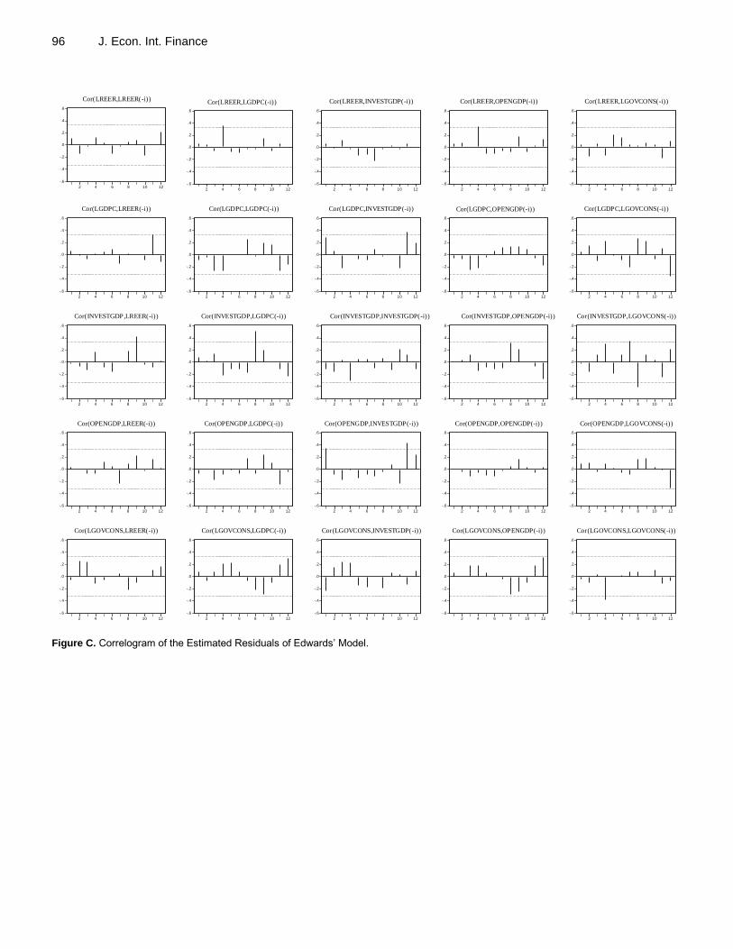
96 J. Econ. Int. Finance

Figure C. Correlogram of the Estimated Residuals of Edwards’ Model.

-.6

-.4

-.2

.0

.2

.4

.6

2 4 6 8 10 12

Cor(LREER,LREER(-i))

-.6

-.4

-.2

.0

.2

.4

.6

2 4 6 8 10 12

Cor(LREER,LGDPC(-i))

-.6

-.4

-.2

.0

.2

.4

.6

2 4 6 8 10 12

Cor(LREER,INVESTGDP(-i))

-.6

-.4

-.2

.0

.2

.4

.6

2 4 6 8 10 12

Cor(LREER,OPENGDP(-i))

-.6

-.4

-.2

.0

.2

.4

.6

2 4 6 8 10 12

Cor(LREER,LGOVCONS(-i))

-.6

-.4

-.2

.0

.2

.4

.6

2 4 6 8 10 12

Cor(LGDPC,LREER(-i))

-.6

-.4

-.2

.0

.2

.4

.6

2 4 6 8 10 12

Cor(LGDPC,LGDPC(-i))

-.6

-.4

-.2

.0

.2

.4

.6

2 4 6 8 10 12

Cor(LGDPC,INVESTGDP(-i))

-.6

-.4

-.2

.0

.2

.4

.6

2 4 6 8 10 12

Cor(LGDPC,OPENGDP(-i))

-.6

-.4

-.2

.0

.2

.4

.6

2 4 6 8 10 12

Cor(LGDPC,LGOVCONS(-i))

-.6

-.4

-.2

.0

.2

.4

.6

2 4 6 8 10 12

Cor(INVESTGDP,LREER(-i))

-.6

-.4

-.2

.0

.2

.4

.6

2 4 6 8 10 12

Cor(INVESTGDP,LGDPC(-i))

-.6

-.4

-.2

.0

.2

.4

.6

2 4 6 8 10 12

Cor(INVESTGDP,INVESTGDP(-i))

-.6

-.4

-.2

.0

.2

.4

.6

2 4 6 8 10 12

Cor(INVESTGDP,OPENGDP(-i))

-.6

-.4

-.2

.0

.2

.4

.6

2 4 6 8 10 12

Cor(INVESTGDP,LGOVCONS(-i))

-.6

-.4

-.2

.0

.2

.4

.6

2 4 6 8 10 12

Cor(OPENGDP,LREER(-i))

-.6

-.4

-.2

.0

.2

.4

.6

2 4 6 8 10 12

Cor(OPENGDP,LGDPC(-i))

-.6

-.4

-.2

.0

.2

.4

.6

2 4 6 8 10 12

Cor(OPENGDP,INVESTGDP(-i))

-.6

-.4

-.2

.0

.2

.4

.6

2 4 6 8 10 12

Cor(OPENGDP,OPENGDP(-i))

-.6

-.4

-.2

.0

.2

.4

.6

2 4 6 8 10 12

Cor(OPENGDP,LGOVCONS(-i))

-.6

-.4

-.2

.0

.2

.4

.6

2 4 6 8 10 12

Cor(LGOVCONS,LREER(-i))

-.6

-.4

-.2

.0

.2

.4

.6

2 4 6 8 10 12

Cor(LGOVCONS,LGDPC(-i))

-.6

-.4

-.2

.0

.2

.4

.6

2 4 6 8 10 12

Cor(LGOVCONS,INVESTGDP(-i))

-.6

-.4

-.2

.0

.2

.4

.6

2 4 6 8 10 12

Cor(LGOVCONS,OPENGDP(-i))

-.6

-.4

-.2

.0

.2

.4

.6

2 4 6 8 10 12

Cor(LGOVCONS,LGOVCONS(-i))

Hosni and Rofael 97

Table 9. Johansen co-integration test.

Unrestricted co-integration rank test

Statistics CV_5% CV_1% No. of CE

Trace Statistics 27.50 29.68 35.65 3

Max. Eigen Value 19.92 20.97 25.52 3

1 Co-integrating Equation

Normalized co-integrating coefficients (reduced form estimates)

LREER LGDPD EXOG GOVCS OPEN LTOT

Estimates 1.00 1.68 -0.36 -1.21 0.10 -5.36

t-statistics -1.59 6.53 2.69 -7.97 6.18

Adjustment coefficients

Δ(LREER) Δ(LGDPD) Δ(EXOG) Δ(GOVCS) Δ(OPEN) Δ(LTOT)

Estimates -0.09 -0.01 3.21 0.29 -2.01 0.01

t-statistics -2.05 -0.21 5.58 3.98 -0.73 1.33

Table 10. Vector error correction estimates.

Estimates t-statistics

Long Run Estimates

LGDPD(-1) -1.68 -1.59

EXOG(-1) 0.36 6.53

GOVCS(-1) 1.21 2.69

OPEN(-1) -0.01 -7.97

LTOT(-1) 5.36 6.18

Constant -21.18

ECM -0.09 -2.05

Short Run Dynamics

Δ(LREER(-1)) 0.22 1.09

Δ(LGDPD_2(-1)) 0.15 0.60

Δ(EXOG(-1)) -0.01 -1.01

Δ(GOVCS(-1)) -0.04 -0.42

Δ(OPEN(-1)) 0.00 0.51

Δ(LTOT(-1)) -0.02 -0.02

Constant 0.06 1.52

DUMEX -0.10 -2.03

DUMCRIS 0.05 1.44