1

Determining the Equilibrium Exchange Rate for Jamaica: A fundamentalist approach for deferring time horizons

DRAFT

James S. J. Robinson1 Research Services Department

Research and Economic Programming Division Bank of Jamaica

June 2010

Abstract This paper investigates the determination of equilibrium exchange rate in Jamaica over the short-

run (SR), medium-run (MR), and long-run (LR) and their potential impact on competitiveness.

For this study, the mean reverting properties of the real exchange rate (RER) is employed as the

metric of equilibrium exchange rate. Three distinct fundamentalist based approaches are used to

evaluate the dynamic process of mean reversion in the RER among the range of theoretically

based impacting variables, utilizing cointegration and decomposition techniques. Key factors

contributing to disequilibrium in the RER were identified within each time frame. Also, the study

yielded some policy recommendations to maintain long term stability of the exchange rate and

prevent the infrequent but disruptive adjustments in the domestic foreign exchange market. The

paper relies heavily on the survey of equilibrium exchange rate models conducted by Driver and

Westaway (2004), supplemented by a range of prominent empirical investigations on pre-selected

models.

1 The views expressed in this paper are those of the author and does not necessarily represent those of BOJ or BOJ policy.

2

TABLE OF CONTENTS 1 INTRODUCTION ...................................................................................................................3

Why Equilibrium Exchange Rates?........................................................................................3 Contextual Overview..............................................................................................................3 Investigative Contribution ......................................................................................................4 Outline of Paper......................................................................................................................5

2 CONCEPTUAL FRAMEWORK............................................................................................5 Exchange Rates Defined.........................................................................................................5 Exchange Rates Parity Conditions..........................................................................................6 Equilibrium Exchange Rate....................................................................................................7

3 LITERATURE REVIEW ........................................................................................................8 Short-Run Models...................................................................................................................8 Medium-Run Models..............................................................................................................9 Long-Run Models.................................................................................................................11 Model Selection....................................................................................................................12

4 DATA DESCRIPTION .........................................................................................................13 5 DATA TREND ANALYSIS .................................................................................................17 6 ECONOMETRIC METHOD ................................................................................................20

CHEER Methodology...........................................................................................................21 BEER Methodology .............................................................................................................22 PEER Methodology..............................................................................................................23

7 ECONOMETRIC RESULTS ................................................................................................24 CHEER Model Results .........................................................................................................24 BEER Model Results............................................................................................................25 PEER Model Results ............................................................................................................29

8. COMPETITIVENESS...........................................................................................................29 Financial Sector Crisis (Mid to Late 1990’s)........................................................................29 Foreign Currency Market Instability (2003).........................................................................30 Global Economic & Financial Crisis (2008) ........................................................................30

9. CONCLUSION......................................................................................................................31 10. BIBLIOGRAPHY..................................................................................................................33 11. APPENDIX ...........................................................................................................................35

3

1 INTRODUCTION Why Equilibrium Exchange Rates?

The level and variability of exchange rate is widely held as a gauge for international

competitiveness and macroeconomic stability. A country’s level and trend in international

competitiveness may establish whether it is or will be a net importer or exporter, borrower or

lender, debt stricken, crisis bound or fundamentally sound. In establishing a sound

macroeconomic environment, a stable exchange rate is needed to build confidence; promote long-

term planning and investment among foreign and domestic stakeholders of a country. The Bank

of Jamaica (BOJ) is charged with the responsibility of maintaining stability within the foreign

currency market toward this end. It becomes crucial for the bank to identify an equilibrium level

of exchange rate to be targeted in carrying out its mandate. This paper seeks to achieve that goal

by identifying the current position of exchange rate relative to the fundamentally determined

equilibrium level. The paper seeks to identify periods of, existing and potential, exchange rate

misalignment signaled by changes in economic fundamentals over varying time spans.

Contextual Overview

Jamaica, a small developing country is a net importer of traded goods and services. The country

relies heavily on foreign currency inflows from Tourism, Remittances, Foreign Direct

Investments, and Bauxite exports. Increased competition and elimination of preferential

privileges among longstanding traditional exports such as banana, and sugar has stimulated

concerns of reduced competitiveness for the nation during the past decade.

Jamaica remains vulnerable to external shocks that affect major export markets and cost of

imported raw materials. A key factor contributing to the cost of production is imported oil that

severely impeded Jamaica’s economic activity in the international oil shocks of the 1970’s and

recently, mid to late 2000’s. In the same time periods, earning from tourism, bauxite exports and

access to foreign financing were contracted resulting in a balance of payments crisis for the

territory. Both periods necessitated reliance on the international monetary fund for financial

assistance. In the early 1990’s the country liberalized its foreign exchange market resulting in

significant depreciation of the local currency. By the mid to late 1990’s, the country experienced

a financial crisis leading to significant public debt accumulation2.

2 The Jamaican financial crisis of the mid to late 1990’s was attributed to significant build up of non-performing loans attributed to poor financial regulation and imprudent business practices. The GOJ opted for a bailout in guiding the economy back to recovery.

4

Jamaica has long strived to become competitive as evidenced by competitive strategies such as

import substitutions, Export promotion, and Liberalization. Nonetheless, the likelihood of balance

of payment crises will increase when negative external shocks result in the deterioration of a

country’s terms of trade. In the case of Jamaica, these included weather related shocks,

significant supply shortage of capital and raw materials such as oil on the international market. A

significant accumulation of debt, similar to Jamaica’s financial crisis in the mid-to-late 1990’s

imposes a risk premium on invested capital, thus reducing the level of competitiveness.

Investigative Contribution

Precursory studies related to exchange rate in Jamaica demonstrate that equilibrium conversion

on the basis of uncovered interest parity (UIP) is evidently weak (see McFarlane 2003). In this

paper, it was incited that prolonged deviation from equilibrium was attributed to a time varying

risk premium ascribed to fiscal dominance in relative asset supplies. In estimating Jamaica’s real

equilibrium exchange rate, Williams (2008) demonstrated that the two normative approaches that

were employed gave conflicting results suggesting a state of over-valued currency in one, and a

state of equilibrium in the other. A third method, being a more positive approach, however

suggested a state of equilibrium3.

The issue surrounding appropriate measure of competitiveness was confronted by Hendry (2001).

It was indicated that the real effective exchange rate (REER) may not adequately capture the level

of competitiveness in Jamaica. He pointed out that depreciation, contrary to typical belief, does

not necessarily lead to an improvement in external competitiveness. The validity of the REER as

a measure of competitiveness was also evaluated by Henry and Longmore (2003) in determining

its impact on elements of Jamaica’s current account. The results show little correspondence of the

REER to current account components and demonstrated that selected exports had insignificant

responses to alterations in the REER. Henry (2001) recommended the use of alternative measures

of competitiveness in conjunction with the REER. These include Unit Labour Cost, Profitability

among Tradables, Ratio of Tradables to Non-tradables, and the ratio of Trade Balance to Total

Trade.

3 Williams (2008) utilized three methods which were the Macroeconomic Balance (MB) approach, the External Sustainability (ES) approach, which are both normative in nature. The last method recognized as the Equilibrium Exchange Rate (ERER) approach is the more positive direct estimation method.

5

Contrary to previous studies, this paper seeks to ascertain the equilibrium state of the RER over

three distinctive time horizons. Inter-temporal contrasts are conducted to determine the current

position and likely direction of the RER relative to the SR, MR, and LR measures of equilibrium.

Acknowledging the misguided perception of RER as a one sided indicator of competitiveness, the

paper adopts methods that explicitly captures both the exchange depreciating and exchange

appreciating increases in competitiveness4. This paper also employs alternative measures of

competitiveness as recommended by Henry (2001) in evaluating misalignment and the steady-

state conversion of Jamaica’s fundamentally determined equilibrium exchange rate over the three

time horizons.

Outline of Paper

Section 2 of this paper follows with a conceptual framework within which equilibrium exchange

rates are evaluated. Section 3 follows with a literature review outlining the crucial elements of

equilibrium exchange rate models grouped within three distinctive time horizons (SR, MR, &

LR). Section 4 gives a description of the data and key fundamental variables and competitiveness

indicators observed in the investigation. Section 5 provides a trend analysis of the key

fundamental variables followed by Section 6 which outlines the econometric methods employed

in carrying out the various empirical analyses. Section 7 presents the econometric results

generated form the range of empirical tests conducted that is immediately followed by Section 8

that evaluate key indicators of competitiveness in relation to periods of disequilibrium. Section 9

concludes with a survey of the interpreted findings within the paper followed by a bibliography

and appendix with key tables and graphs.

2 CONCEPTUAL FRAMEWORK Exchange Rates Defined

Mishkin (2004) defines exchange rate as “the price of one currency in terms of another”. This is

also regarded as the nominal exchange rate. A real exchange rate can be expressed as the

nominal exchange rate adjusted for any price differences between two or more countries.

Depending on the prices being observed for the two countries (trade prices, consumer prices,

wholesale prices, producer prices, GDP deflators, labour costs etc), the measurement of real

exchange rate can take on very different values and direction of change and interpretation. The 4 There are instances when competitiveness can be enhanced from rising productivity. In such cases the exchange rate appreciates from an increase in the demand for domestic currency. This contradicts the common perception that in order to become more competitive, the exchange rate has to depreciate.

6

real exchange rate (RER) can be expressed in the manner shown in equation 1. A representation

of the real effective exchange rate (REER) is derived from a composite weighting of the RER for

a range of key trading partners. This is expressed in equation 2 below:

)/( *jtitijt PPSRER =

[ ]∏=

=n

j

ijjtitijt PPSREER

1

*/ ω

Where RER and REER is the real exchange rate and real effective exchange rate respectively;

tS is the nominal exchange rate between country i and j; itP is the price level for the domestic

country i and *jtP is the price level for the foreign country j.5 The real exchange rate is expressed

as a geometric mean where ijω is the weight of the foreign country j in the total trade of country i.

Exchange Rates Parity Conditions

There are two fundamental bases on which theorists believe exchange rate adjustments are made.

These include the Purchasing Power Parity (PPP) and the Uncovered Interest Parity (UIP).

Formally stated, Purchasing Power Parity (PPP) is based on the Law of One Price which implies

that, in two countries that produce a similar good with minimal transportation costs and barriers

to trade, the exchange rate should be such that the cost of a non-differentiable good remains the

same throughout the world irrespective of the country in which it is produced (Mishkin 2004).

PPP extends this law of one price to require that any adjustments in the price or cost of producing

the particular good will result in an appropriate adjustment in the exchange rate to ensure that the

law of one price holds.

Uncovered Interest Parity (UIP) is based on the Theory of Asset Demand assuming currency

transfers between territories are free of capital mobility restrictions rendering deposits in foreign

currency to be a perfect substitute for deposits in domestic currency. On this basis the decision

about whether to hold foreign or domestic currency deposits will depend solely on the rate of

interest offered on either domestic or foreign currency deposit accounts. Both domestic and

foreign investors will shift deposits to the territory that offers a higher rate of interest on their

respective currency deposits. The uncovered interest parity condition therefore requires that the

5 Real effective exchange rate (REER) is contrasted to the bilateral exchange rate which is the exchange rate between the domestic country and a single foreign country. Like the REER, it is normally expressed as the quantity of foreign currency it takes to acquire one unit of the domestic currency. Hence an appreciation is represented as an increase in the exchange rate while depreciation is reflected as a reduction.

(1)

(2)

7

exchange rate be adjusted to correct any prevailing interest rate deviations (arbitrage) between the

observed territories.

Equilibrium Exchange Rate

The conditions of PPP and UIP are essentially equilibrium conditions that identify the ideal level

of exchange rate between a domestic economy and its trading counterpart. The PPP condition

holds when the exchange rate is such that the price of a local good is indifferent to the price of an

identical foreign good. The UIP condition holds when the exchange rate is such that the interest

return on domestic currency is indifferent to the interest return on foreign currency deposits. The

key difference between the two is that PPP is essentially a long-run (LR) condition due to

stickiness of prices over time, while UIP is a short-run (SR) equilibrium condition due to the

lower level of friction in capital market interest rates determination.

From a theoretical perspective, SR models emphasize equilibrium exchange rate based on rational

market behaviour in light of all available information6. MR models emphasize the attainment of a

sustainable internal and external trade balance; while the LR models emphasize the structural role

that fiscal debt stock and stock flow adjustments will play in determining the equilibrium

exchange rate.

It is important to identify an equilibrium exchange rate for two main reasons. They are: (1) the

effective monitoring and targeting (monetary policy) of a desired real exchange rate for stability

in the foreign currency market; and (2) preserving the level of competitiveness of key export

sectors (industries) based on relative import costs and export price with a focus on enhanced

productivity and a sustainable balance of payment position. This paper seeks to address both

areas of concern in the analysis stemming from the determination of Jamaica’s equilibrium

exchange rate.

In an extensive survey investigating the concepts of equilibrium exchange rates, Driver and

Westaway (2004) expressed the structural form commonly used to explore equilibrium

relationships between an exchange rate and the wide cross-section of fundamental and transitional

variables. The structure is expressed in equation 3 below.

6 There are also statistical methods that seek to decompose permanent components from trends in exchange rates. Such models rely on the condition of convergence for proof of equilibrium and are less applicable when a specific equilibrium level is sought after.

8

tttt TZe εθβ +′+′=

Where te represents the specified exchange rate at time period t, tZ is a vector of MR and LR

economic fundamental variables identified by theory, tT is a vector of transitional variables

encompassing lagged dependent, independent and other variables utilized to capture the SR

dynamics of the specification. Both β ′ and θ ′are coefficient vectors for the respective

fundamental and transitional variables.

3 LITERATURE REVIEW

Short-Run Models

Short-run equilibrium exchange rate is projected from a combination of actual fundamental

variables and anticipated transitional variations. The SR equilibrium exchange rate is therefore

that estimated rate for which unexpected variations ( tε ) are abstracted out. Driver and Westaway

(2004) specify the SR structure of the equilibrium exchange rate as shown below in equation 4.

ttSRt TZe θβ ′+′=

SR models largely consider capital market dynamics that reflect the actions of asset holders in

response to available market information. The theoretical condition that describes this type of

response from market participants is the UIP. The range of SR models available for this analysis

include the: Flexible Price Monetary Models (FPMM); Sticky Price Monetary Models (SPMM)

proposed by Dornbusch (1976); Portfolio Balance model presented by Frankel (1993),

MacDonald and Taylor (1992) and Taylor (1995); the Capital Enhanced Equilibrium Exchange

Rate (CHEER) model presented by MacDonald (2000); and the Behavioral Equilibrium

Exchange Rate (BEER) model presented by Clark and MacDonald (1997 and 1999).

The modeling of equilibrium exchange rate has been widely assessed in economic literature. The

FPMM was made popular in the early 1970’s post Brenton-Woods shift towards floating

exchange rate regimes in the industrialized world: see Rapach and Wohar (2001) and Moura et al

(2008). The FPMM proposed that prices are flexible and that PPP holds continually; see Frankel

(1976) and MacDonald (1992). The poor performance of the FPMM however, led to the

recommendation of alternative strategies for explaining foreign exchange rate movements.

Dornbusch (1976) introduced the concept of sticky prices, suggesting that prices take time to

(3)

(4)

9

adjust, thereby causing nominal and real exchange rates to overshoot equilibrium levels.

Dornbusch (1976) showed that with distorted interest rates, exchange rates eventually revert to

the PPP equilibrium level based on the velocity of price adjustments.

There are however, other shortcomings that the FPMM and SPMM did not address. Of key

concern is the UIP assumption of no restrictions on the mobility of capital between territories.

Evidence in support of: home bias, liquidity difference, solvency risk, tributary differences, and

the presence of currency exchange rate risks supports the notion of imperfect substitution of

assets across borders; see Moura et al (2008). The PBMM was therefore established to remedy

the asset market limitation encountered. The model also incorporated stock-flow effects, such as

current account misalignments in explaining equilibrium exchange rates (see MacDonald, 1992).

The CHEER model is based on the premise that, at any given point in time, the PPP condition

may be in disequilibrium due to non-zero interest rate differentials7 in the SR. The CHEER model

combines both components of the PPP and UIP conditions in determining equilibrium exchange

rates. Whereas the PBMM utilized a risk premium to capture the effects of imperfect capital

mobility, the CHEER instead utilizes the price differentials. The BEER model is also premised

on the UIP condition which accounts for imperfect capital mobility with a risk premium. In this

analysis, Clark and MacDonald (1997 and 1999) used other variables regarded as fundamentals to

explain variations in the RER.

Medium-Run Models

An exchange rate is theoretically deemed to be at MR equilibrium when the internal and external

economic affairs of a country are brought to a point where there is no natural tendency for change

(balance or steady state)8. The internal balance relates to a position of full employment of

resources while external balance relates to a sustainable current account position that is typically

consistent with convergence to a LR steady state of stock flow9. At the MR level, all “nominal

inertia would have been washed out of the system” as noted by Driver and Westaway (2004).

This essentially nullifies unexplained and transitional forces on the equilibrium exchange rate

rendering its determination wholly on the basis of estimated medium term economic

7 It is postulated that when interest rate differentials are non-zero, and are needed to finance the capital account, it could result in disequilibrium in the PPP determined real exchange rate. Driver and Westaway (2004) p.37. 8 Internal full employment is otherwise regarded as the Non Accelerating Inflation Rate of Unemployment (NAIRU). 9 The term “stock” in the literature refers to the public debt stock of a country while “stock-flows” refer to the fiscal surplus or deficit that will determine the future accumulation or diminishing of indebtedness.

10

fundamentals10. This measure coincides with the concept of flexible price equilibrium that is

independent of interventionist type policies. Inline with the structure presented in equation 5, the

MR equilibrium is expressed as follows:

tMRt Ze ˆβ ′=

The range of MR models contemplated for this analysis include the: Fundamental Equilibrium

Exchange Rate (FEER) model investigated by Wren-Lewis (1989 and 1992); and the Desired

Equilibrium Exchange Rate examined by Artis and Taylor (1993). The BEER method is also

contemplated for the MR analysis though employing less subjective approaches to establishing

internal and external balance.

The internal and external balance conditions for the FEER are premised on the optimal levels of

capital flow (K) and current account (CA) balance demonstrated by Clark and MacDonnald

(1998). Faruqee, Isard, and Masson (1998) also show that the difference between savings and

investment will reflect this balance. It is demonstrated that any deviation from the estimated CA

and the actual CA after considering seasonal trends and specification errors, will unveil that

FEER that is required to maintain some optimal level of the income and savings condition. The

term Desired Equilibrium Exchange Rate (DEER) is another name for the FEER that highlights

the normative characteristic of the model, see Bayoumi et al (1994) and Artis and Taylor (1993).

The FEER / DEER methodology is characterized as normative11 in a sense that the indicators of

internal and external balance are calculated to derive ideal/optimal/desired levels. The optimal

calculations are then superimposed in the determination of an equilibrium exchange rate. A

representation of the FEER was conducted for Jamaica by Williams (2008) using two established

methods of calculating equilibrium norms12. The results yielded inconsistent results where one

method, the external sustainability approach (ES), alluded to a state of equilibrium and the other,

macroeconomic balance approach (MB), a significant overvaluation. A BEER model was also

estimated which suggested that Jamaica was in a state of MR equilibrium, consistent with the

External Sustainability approach.

10 Driver and Westaway (2004) suggest that the premise on which equilibrium exchange rate is wholly dependent on fundamental variables is only valid if there are no significant hysteresis effects and that adjustments take place within the reasonably short run. 11 The normative method of the FEER is considered by some a limitation since the ideal levels are superimposed by the investigator by a calculated means. The normative nature of FEER is alluded to by the founder Williamson (1994) and other seminal papers such as Clark & MacDonald (1998), p.6, and Driver & Westaway (2004) p.46. 12 These two methods included the Partial Macroeconomic Balance (MB) approach suggesting disequilibrium while the External Sustainability (ES) approach suggested a stable exchange rate.

(5)

11

In an assessment of extensions to the Macroeconomic Balance Approach, Isard, Faruqee and

Debelle (1998) demonstrated that both a partial adjustment model and error correction model

generated satisfactory explanations of the CA behavior in relation to various explanatory

affecting the savings and investment balance. Clark and MacDonald (1998), however, points out

that, unlike the BEER approach, the FEER has no theoretical basis on which a convergence to

equilibrium is explained. Rather the FEER is simply a method of calculating an equilibrium

exchange rate given optimal levels of the CA and Savings & Investment balance. Any adjustment

to the exchange rate is then assumed depending on the relative position of the actual exchange

rate to the calculated equilibrium rate.

This paper is focused on the less-normative methods of estimating the equilibrium path of the

REER. In light of this, the BEER is used to estimate the behavioral impact of MR and LR and

Transitional variables on the REER. Among the list of LR variables are joint relationships that

will establish equilibrium by imposing parameter restrictions. Cointegration and Error Correction

techniques are employed to arrive at the results.

Long-Run Models

LR equilibrium exchange rate is considered to be the level consistent with equilibrium stock-

flows. At this stage, there are no endogenous tendencies for change, such that all MR related

bubble, and cyclical effects nullified (see Driver & Westaway 2004). The LR equilibrium

expression is presented in equation 6, where the bar represents the LR state of variables.

tLR

t Ze β ′=

In the literature, two predominant methods are utilized in observing LR equilibrium exchange

rates. They include (1) the purely statistical approach where focus is placed on the decomposition

of a permanent component of the exchange rate trend; and (2) the fundamentals approach, which

seeks to explain equilibrium exchange rate based on a desirable (steady state) level of capital or

stock-flow expected to be attained in the long-haul.

The models explored for conducting the LR analysis include the Natural Real Exchange Rate

(NATREX) approach presented by Stein (1994), Stein and Allen (1995), and Stein and Paladino

(1998); the Permanent Equilibrium Exchange Rate (PEER) model, and the Structural Vector

Autoregression (SVAR) model utilized by Clarida and Gali (1994).

(6)

12

The NATREX approach is an offshoot of the FEER which incorporates the impact of

fundamental variables on the equilibrium exchange rate. The method also incorporates the

portfolio balance condition that domestic and international real interest rates are aligned. The

NATREX can be used for either MR or LR analysis. After estimation, the equilibrium level is

derived from setting residuals equivalent zero. Where as NATREX takes on the normative

methods employed by the FEER and removes random transitory effects, the PEER instead utilizes

the more positive BEER model from which the equilibrium REER is derived from a permanent

decomposition of the estimated results.

The SVAR model is useful in identifying key shocks that have and are likely to affect the real

exchange rate. The method however, cannot provide a reliable equilibrium exchange rate level

due to starting point limitations. Emphasis is therefore placed on the fundamentals based

approach, and in particular the BEER method following which the permanent component is

decomposed to reveal an equilibrium REER path. This method of estimating the PEER is adopted

from Fernandez et al (2001).

Model Selection

The selection of models is based on conformity to the criteria of being fundamentally determined.

Additionally, data accessibility will confine research to those models for which adequate data

representation can be attained. For the purpose of this paper, the BEER method was employed for

both SR and MR analysis and also combined with the PEER method to determine a LR

permanent component. The FEER methods were rejected on the basis of inconsistent results

presented on the case of Jamaica (see Williams 2008), and the less than positive approach

employed in the investigation. The methods employed by Clark & MacDonald (1998), and

Melecky & Komarek (2005) is adopted for the SR and MR BEER determination.

The method employed by Fernandez et al (2001), utilized the BEER estimation technique to

explain the RER following which the transitory and permanent components were decomposed.

The Permanent component is considered the LR PEER that will unveil periods of over and

undervaluation when compared to the original RER.

13

4 DATA DESCRIPTION

Monthly data is used for the period April 1995 to July 2009. The Nominal Exchange Rate (NER)

is used to model the SR CHEER Model while the Real Exchange Rate is (RER) used as the

dependent variable for the BEER and PEER models The RER is adjusted expressed as the NER

adjusted by the ratio of foreign and domestic consumer prices. RER are expressed in foreign

dollars per unit of domestic dollars. Resultantly, any increase in the RER represents an

appreciation. The NER however is represented as domestic dollars per foreign dollar. In this case

an increase is synonymous to depreciation.

Domestic Price (PRID) - Domestic prices are used to capture the impact of inflation on exchange

rates. The transmission may either be by a substitution or income effect. As it pertains to the

former, when domestic prices increase, local consumers are expected to shift demand away from

the more expensive domestic goods to the relatively cheaper foreign goods. In such

circumstances, the demand for domestic currency decline resulting in depreciation. The income

effect reflects a greater demand for the domestic currency to maintain the same level of

consumption. As such, domestic inflation would result in an appreciation. The domestic price

(PRID) is the log of Jamaica’s Consumer Price Index (CPI).

Foreign Price (PRIF) - Foreign prices, like domestic prices also affects the exchange rate by

transmission of the substitution and or income effect. By substitution, an increase in foreign

prices, will trigger an increase in the demand of relatively cheaper domestic goods away from the

more expensive foreign goods. In this case, more domestic currency is demanded relative to the

foreign currency resulting in an appreciation of the domestic currency. The income effect reflects

a greater demand for the foreign currency to maintain the same level of consumption. As such,

foreign inflation would result in a depreciation of the domestic currency. In this paper, the log of

US Consumer Price Index is used for the foreign price (PRIF).

Domestic and Foreign Interest Rates (INTD & INTF) - Interest rates are expected to have a direct

impact on currency holdings. Higher domestic interest rates, all things being equal, are expected

to result in both domestic and foreign investors shifting holdings away from foreign currency

deposits to domestic currency depost. When foreign interest rates increase, the opposite effect of

a rising domestic interest rate becomes true. The domestic interest rate used for this paper is

14

Jamaica’s 6 month annualized Treasury bill rate in decimals. The foreign interest rate taken as

the US 6-month annualized Libor rate is used for the purpose of this paper.

Interest Rate Differential (RIRD) [negative] – Trends in the interest rate differential is expected to

capture the uncovered interest parity (UIP) condition which suggests that portfolio investors will

shift capital to a territory with relatively higher interest rates. The UIP condition requires that the

exchange rate adjusts to prevent any arbitrage emerging from interest rate differentials between

territories. Therefore, an increase in the Jamaican interest rates (INTD) relative to that of the US

interest rate (INTF) would attract investors away from USD to JMD denominated holdings

(deposits). Naturally the demand for JMD would increase causing a domestic (JMD) appreciation.

However, the theory of UIP requires that the exchange rate will adjust to nullify any arbitrage and

thereby prevent significant shifts in portfolio balances of either domestic or foreign denominated

currencies. The real interest rate differential (RIRD) is derived from the INTD net of Jamaica’s

12 month headline inflation rate minus the INTF net of the US 12-month inflation rate.

Net Foreign Asset (NFA) [positive] – The impact of the LNFA on the exchange rate is considered

from two perspectives. From a portfolio balance perspective, a current account deficit or

worsening thereof will require financing from international investors who will demand higher

yields which can only be achieved by exchange rate depreciation if interest rates are taken as

given. Therefore deterioration (decline) in the LNFA by way of increased foreign currency

liability should lead to depreciation (decline) in the RER and vice versa in light of the portfolio

balance effect. The alternative reasoning is that debt attained to finance CA deficits will attract

interest payments. It is only by way of an improved trade balance that premiums can be afforded.

This will require a depreciation of the domestic currency in order to increase competitiveness,

improve the trade balance, and hence, ability to service such loans. The LNFA is calculated as the

total foreign assets held by Jamaica’s Central Bank, Commercial Bank & Central Government in

millions of USD minus total foreign liability held by the same institutions. The values are then

expressed in logs after normalizing by way of adding 1 million to each value considering all

values are negative where Jamaica is a net borrower.

Net Government Debt Differential (LNGDD) [positive] – This risk premium is included in SR

models to take account of limitations associated with presence of imperfect mobility of capital

across borders. When domestic debt increases relative to foreign denominated debt, the domestic

risk premium will increase. Since investors require higher compensation for this added risk, if

15

interest rates are given, then the domestic currency will depreciate. For the purpose of this paper

LNGDD is expressed as the log of total GOJ and BOJ domestic debt in millions of USD minus

the log of total foreign debt liabilities held by the same institutions in millions of JMD.

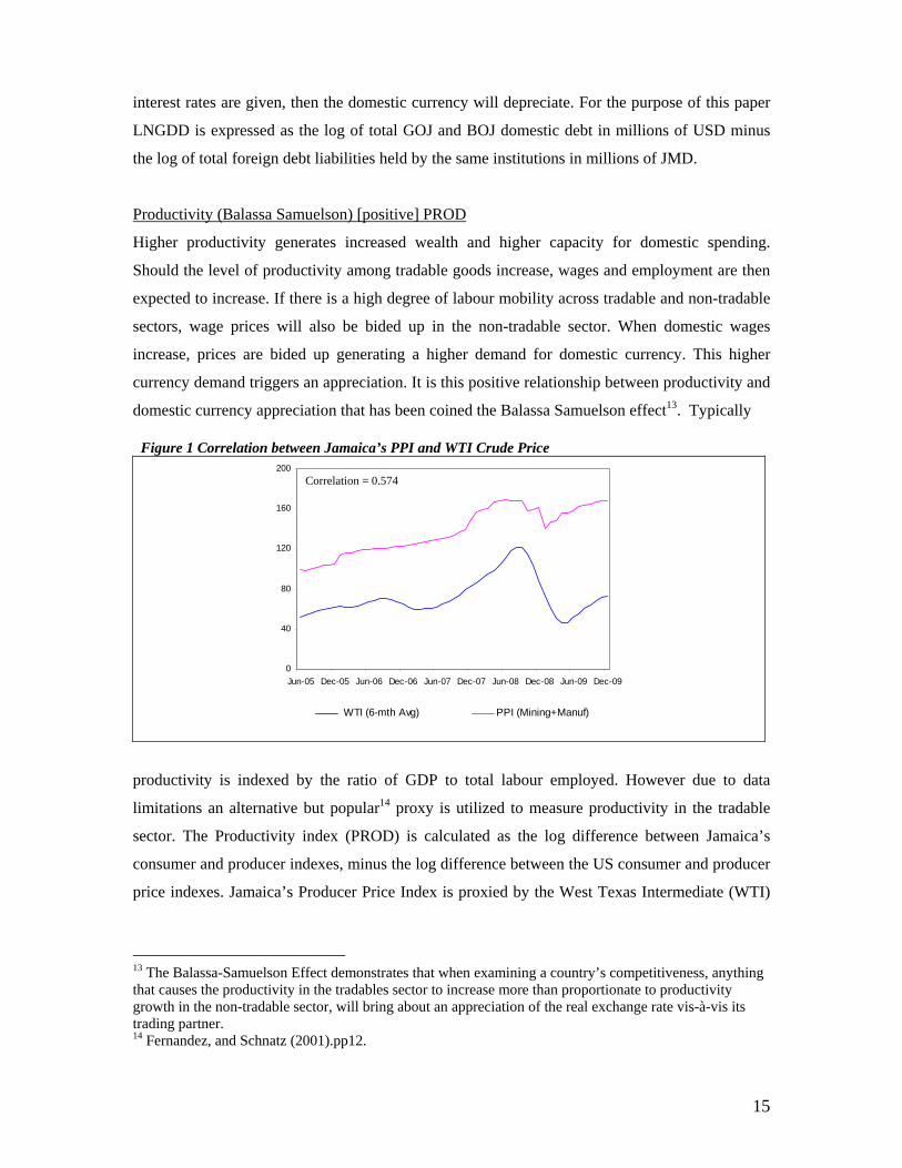
Productivity (Balassa Samuelson) [positive] PROD

Higher productivity generates increased wealth and higher capacity for domestic spending.

Should the level of productivity among tradable goods increase, wages and employment are then

expected to increase. If there is a high degree of labour mobility across tradable and non-tradable

sectors, wage prices will also be bided up in the non-tradable sector. When domestic wages

increase, prices are bided up generating a higher demand for domestic currency. This higher

currency demand triggers an appreciation. It is this positive relationship between productivity and

domestic currency appreciation that has been coined the Balassa Samuelson effect13. Typically

productivity is indexed by the ratio of GDP to total labour employed. However due to data

limitations an alternative but popular14 proxy is utilized to measure productivity in the tradable

sector. The Productivity index (PROD) is calculated as the log difference between Jamaica’s

consumer and producer indexes, minus the log difference between the US consumer and producer

price indexes. Jamaica’s Producer Price Index is proxied by the West Texas Intermediate (WTI)

13 The Balassa-Samuelson Effect demonstrates that when examining a country’s competitiveness, anything that causes the productivity in the tradables sector to increase more than proportionate to productivity growth in the non-tradable sector, will bring about an appreciation of the real exchange rate vis-à-vis its trading partner. 14 Fernandez, and Schnatz (2001).pp12.

Figure 1 Correlation between Jamaica’s PPI and WTI Crude Price

0

40

80

120

160

200

Jun-05 Dec-05 Jun-06 Dec-06 Jun-07 Dec-07 Jun-08 Dec-08 Jun-09 Dec-09

WTI (6-mth Avg) PPI (Mining+Manuf)

Correlation = 0.574

16

crude oil price due to the limited time-span available for the PPI15. The PPI reflects the simple

average of both the Mining and Manufacturing Producer Price Indexes for Jamaica. The

correlation between Jamaica’s monthly PPI and the 6-month average of the WTI is 0.57 (See

Figure 4.1).

Terms of Trade [positive] TOT is an indicator of the degree of competitiveness between trading

partners. A country that depends heavily on oil, for instance, might experience deterioration in its

TOT if oil prices should increase whereas; an oil exporting trading partner would experience an

improvement in its TOT. The theoretical underpinnings suggest that a change in the TOT has

both income and substitution effects on the exchange rate, see Melecky & Komarek (2005).

Consider a case where the price of exported goods increased causing an improvement in the

domestic TOT. The substitution effect suggests that domestic producers will drive production

among tradables and away from non-tradables. The resulting wage increases that follow, spurs

demand across both tradables and non-tradables. The higher prices and boost in the current

account that follows will stimulate an appreciation of the domestic currency. The Income effect

emerges when a rebalancing adjustment of the exchange rate takes effect to restore internal

equilibrium between both tradables and non-tradables. The TOT variable is expressed as the ratio

of BOJ’s export index to the import index. The variable is then logged for consistency.

The following variables recommended by Henry ( ) were used in the analysis as a measure of

competitiveness. Due to data limitations, the analysis of competitiveness within Jamaica is

restricted to quarterly trends for the time period March 1998 to December 2009. The variables

include Unit Labour Cost (ULC), Ratio of Tradables to Non Tradables (TNT), and Trade Balance

to Total Trade (TBT). Details are provided below:

Real Effective Exchange Rate (REER) - The REER as defined in equation 2 is actively used as a

measure of competitiveness by the Bank of Jamaica. Jamaica’s REER is the geometric mean of

bilateral exchange rates weighed against the largest 10 trading partners (see equation 1). The

REER is expressed as the cost of one local dollar in terms of the weighted foreign currencies

thereby representing an appreciation when increased and depreciation when reduced. The REER

is typically used as a measure of competitiveness whereby an increase (appreciation) in general

terms signifies a decrease in competitiveness and the inverse, an increase in competitiveness.

15 Jamaica’s Producer Price Index (PPI) has its first data point in January 2005 and is available on a monthly frequency.

17

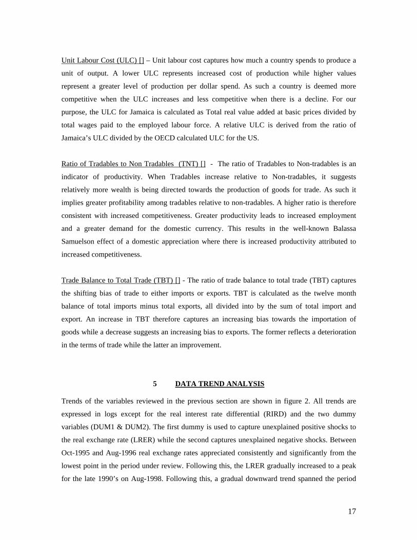
Unit Labour Cost (ULC) [] – Unit labour cost captures how much a country spends to produce a

unit of output. A lower ULC represents increased cost of production while higher values

represent a greater level of production per dollar spend. As such a country is deemed more

competitive when the ULC increases and less competitive when there is a decline. For our

purpose, the ULC for Jamaica is calculated as Total real value added at basic prices divided by

total wages paid to the employed labour force. A relative ULC is derived from the ratio of

Jamaica’s ULC divided by the OECD calculated ULC for the US.

Ratio of Tradables to Non Tradables (TNT) [] - The ratio of Tradables to Non-tradables is an

indicator of productivity. When Tradables increase relative to Non-tradables, it suggests

relatively more wealth is being directed towards the production of goods for trade. As such it

implies greater profitability among tradables relative to non-tradables. A higher ratio is therefore

consistent with increased competitiveness. Greater productivity leads to increased employment

and a greater demand for the domestic currency. This results in the well-known Balassa

Samuelson effect of a domestic appreciation where there is increased productivity attributed to

increased competitiveness.

Trade Balance to Total Trade (TBT) [] - The ratio of trade balance to total trade (TBT) captures

the shifting bias of trade to either imports or exports. TBT is calculated as the twelve month

balance of total imports minus total exports, all divided into by the sum of total import and

export. An increase in TBT therefore captures an increasing bias towards the importation of

goods while a decrease suggests an increasing bias to exports. The former reflects a deterioration

in the terms of trade while the latter an improvement.

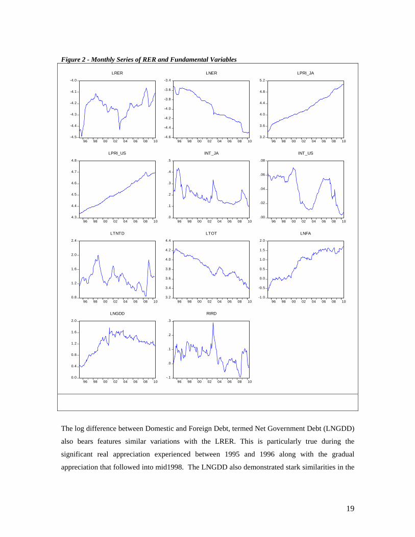
5 DATA TREND ANALYSIS Trends of the variables reviewed in the previous section are shown in figure 2. All trends are

expressed in logs except for the real interest rate differential (RIRD) and the two dummy

variables (DUM1 & DUM2). The first dummy is used to capture unexplained positive shocks to

the real exchange rate (LRER) while the second captures unexplained negative shocks. Between

Oct-1995 and Aug-1996 real exchange rates appreciated consistently and significantly from the

lowest point in the period under review. Following this, the LRER gradually increased to a peak

for the late 1990’s on Aug-1998. Following this, a gradual downward trend spanned the period

18

Aug-1998 to Dec-2002 (4.3 yrs) characterized by moderate oscillations. Between Dec-2002 and

May-2003 the LRER experienced a steep falloff venturing close to the lowest level experienced

in Oct-1995. Following this, the real exchange rate reverted to a strong upward trend over the

period May-2003 to Jul-2005 (2.3 years). The real exchange rate then remained relatively stable

over the period Jul-2005 to Oct-2007 (1.5 years). Immediately following this relative stability, the

real exchange rate appreciated with a significant and consistent slope over the 12-month period of

Oct-2007 to Oct-2008. After the period of relative stability the LRER continued to appreciate

consistently peaking within 12 months in October 2008 while hovering within that range for the

remainder of 2008. However, in the first two months of 2009, there was a drastic depreciation of

the real exchange rate to levels consistent with the one year stability observed during mid 2005 to

late 2007.

The trends in Tradable to Non-tradable Difference (LTNTD) bears close resemblance to the

LRER. The steep and gradual appreciation during the mid to late 1990’s characterized by

corresponding movements in the LTNTD. When the LRER reverted to a gradual downward tend

in latter half of 1998, the LTNTD overshoot this trajectory and only reverted to a downward trend

(12 months later) in late 1999. Following this, the LTNTD gradually declined as did the LRER

for the next 2 ½ years beginning in Nov-1999. The LTNTD, however, severed ties with the

LRER in mid 2002 when a steep increase in the LTNTD was eventually fallowed by the drastic

falloff of the LRER in the first 5 months of 2003. As the LRER begun a strong recovery by

appreciating, the LTNTD (5 months later) started gradually declining against the gradual

appreciation of the LRER for a period of 3 years ending July 2006. Following this, the LTNTD

and LRER was once more synchronized with the exception of the 2 month LRER correction

observed at the start of 2009 which appeared as a gradual adjustment in the LTNTD since.

The Terms of Trade (LTOT) depicted a general upward trend for the major part of the data set.

Nonetheless, the trend reflected slight oscillations and some cyclical shifts over the range. The

LTOT demonstrated no coincidental movement with the LRER in the 1995 to 1996 period when

the LRER appreciated drastically. Nonetheless, following this period, variations in the LTOT

appeared to move in direct opposition to the LRER for the 6 year period to 2002 end. Following

the strong depreciation of the LRER in the first 5 months of 2003, the LTOT and the LRER have

since moved in harmony with the LTOT leading the LRER by approximately 5 months. This was

evidenced in the strong appreciation in the 12 months to Oct-2008 and the sharp corrective

depreciation that followed.

19

Figure 2 - Monthly Series of RER and Fundamental Variables

-4.5

-4.4

-4.3

-4.2

-4.1

-4.0

96 98 00 02 04 06 08 10

LRER

-4.6

-4.4

-4.2

-4.0

-3.8

-3.6

-3.4

96 98 00 02 04 06 08 10

LNER

3.2

3.6

4.0

4.4

4.8

5.2

96 98 00 02 04 06 08 10

LPRI_JA

4.3

4.4

4.5

4.6

4.7

4.8

96 98 00 02 04 06 08 10

LPRI_US

.0

.1

.2

.3

.4

.5

96 98 00 02 04 06 08 10

INT_JA

.00

.02

.04

.06

.08

96 98 00 02 04 06 08 10

INT_US

0.8

1.2

1.6

2.0

2.4

96 98 00 02 04 06 08 10

LTNTD

3.2

3.4

3.6

3.8

4.0

4.2

4.4

96 98 00 02 04 06 08 10

LTOT

-1.0

-0.5

0.0

0.5

1.0

1.5

2.0

96 98 00 02 04 06 08 10

LNFA

0.0

0.4

0.8

1.2

1.6

2.0

96 98 00 02 04 06 08 10

LNGDD

-.1

.0

.1

.2

.3

96 98 00 02 04 06 08 10

RIRD

The log difference between Domestic and Foreign Debt, termed Net Government Debt (LNGDD)

also bears features similar variations with the LRER. This is particularly true during the

significant real appreciation experienced between 1995 and 1996 along with the gradual

appreciation that followed into mid1998. The LNGDD also demonstrated stark similarities in the

20

appreciation observed in the 12-month period to Oct. 2008 and the sharp fall off in the first two

months of 2009. Like the LTNTD, the LNGDD also overshoot the gradual appreciation in the

LRER by approximately 12-months up to late 1999. Over the period 2000 to 2003, the LNGDD

declined gradually inline with the LRER in like manner to the LTNTD. The sharp real

depreciation of the LRER that spanned the first 5 months of 2003 was not featured in the

LNGDD but the corrective appreciation that followed was however reflected in the LNGDD.

The net of total foreign asset to total foreign liability in Jamaica, termed Net Foreign Asset

(NFA), displayed key correlations when compared to the LRER. In the 7 month period between

Nov-1995 and Jun-1996 when the LRER reflected a significant appreciation, the LNFA displayed

a consistent but moderate upward trend that had already been in motion the start of the series.

When the appreciation of the LRER in late 1996 slowed to a moderate increase, the LNFA

switched to a relatively stability that lasted for approximately 3 ½ years to the close of the

decade. At the beginning of 2000 when the LRER had already been following a moderate

depreciation for approximately 12 months, the LNFA started a moderate increase against the

LRER continuing depreciation. By January 2003 when the LRER suffered a sharp depreciation

over 5 months, the LNFA followed with a decline. Thereon, the LNFA remained relatively stable

until another notable decline that manifested in approximately 5 months prior to the sharp

depreciation of the LRER in only 2 months.

The real interest rate differential (RIRD) varies inversely to the LRER during the 3 main periods

of significant LRER changes. These included the 12 month period of depreciation followed by

appreciation between both Jul-1995 and Jun-1996, and Jan-2003 to Dec-2003, and the

appreciation followed by depreciation observed between Oct-2007 to Feb-2009. Throughout the

period of investigation the RIRD displayed continuous oscillations also reflecting inverse

correlations when compared to less pronounced variations in the LRER. This is consistent with

the expected negative relationship between LRER and RIRD as proposed by the theory of UIP.

6 ECONOMETRIC METHOD

Both the CHEER and BEER empirical investigations utilized cointegration techniques that are

outlined in steps 1 to 4 below. Step 5 represents the additional step employed having complete the

BEER investigation to arrive at results for the PEER.

21

(1) Conduct unit root tests on the range of variables to ensure valid properties of the selected

series estimation

(2) Determine the appropriate equilibrium specification using Transitional variables and the

given MR and LR variables.

(3) Conduct Cointegration tests on the MR and LR variables accounting for any additional

exogenous variables.

(4) Estimate the Vector Error Correction Model (VECM) and demonstrate credible results based

on sign of cointegrating parameter, speed of convergence, and strength of exogeniety among

other variables.

(5) Decompose the Transitional and Permanent component for joint BEER and PEER method.

CHEER Methodology

The CHEER model adopted for this paper follows the investigative approach of MacDonald &

Marsh (1997). The CHEER enhances the PPP condition with components that are responsive to

capital market dynamics. This is represented in equation (4).

tttttt IIPPNER εββββ +−+−= *43

*21

Where:

tNER = column vector of spot exchange rate between the US and JA16.

tP = vectors of domestic consumer prices in logs *

tP = vectors of foreign consumer prices in logs

tI = vectors of annualized 3 month domestic interest rate *tI = vectors of annualized 3 month foreign interest rate

kβ = coefficients vectors of the CHEER specification for k = 1 to 4.

tε = the random disturbance component.

All variables are expressed in logs except for domestic and foreign interest rates that are

represented in decimals. Stationarity tests are first conducted on the range of variables as a

prerequisite for cointegration analysis. The commonly used Aumented Dickey Fuller and Phillips

Perron tests were used for this purpose. A range of diagnostic tests are then conducted on varying

deterministic components. Tests for no serial correlation and normality in the errors, required for

appropriate error correction methodologies are also implemented. The number of cointegrating

vectors is then evaluated by way of the Johansen trace and maximum eigen values. Multiple

16 Measured as USD per JMD, therefore an increase represents an appreciation.

(7)

22

cointegrating vectors would require the Johansen maximum-likelihood procedure in appropriately

estimating error correction. Otherwise the standard Engel Granger methodology would suffice.

The sign and significance of the cointegrating coefficient is then evaluated for proof and speed of

error correction in the specified model. With proof of error correction, the VECM residual is

tested for white noise and significance of constant and trend. The cointegrating coefficient is

expected to remove all information from the residuals leaving a white noise and no significant

constant or trend. At this stage the estimated component of the cointegrating equation,

considered to be the equilibrium, is then decomposed and compared to the actual exchange rate.

Any deviations between the two (equilibrium and actual exchange rate) is labeled the exchange

rate misalignments as implied by the proposed model (CHEER).

In accordance with MacDonald and Marsh (1997), a number of restrictions are performed on the

cointegrating equation (beta matrix) to test for evidence of PPP and the relevance of domestic and

foreign interest rate inclusion. Establishing the adequacy or limitations of the model will aid in

assessing the term, direction, and leading factors associated with misalignments in the applicable

exchange rate.

BEER Methodology

The BEER model employed was based on the methods employed by Clark and MacDonald

(1998). The recommend structural form of the BEER model derived from equation (8) is also

represented in equation 9.

ttttt TZZRER εγββ +++= 2211

tttt TBEERRER εγ ++=

where:

tRER = column vector of Jamaica’s US-bilateral real exchange rate

tZ1 = vectors of LR fundamental variables

tZ 2 = vectors of MR fundamental variables

1β , 2β = coefficients vectors of the equilibrium specification.

tT = vector of transitory factors γ = reduced form coefficient vector.

tε = the random disturbance component.

(8)

(9)

23

Congruent with Clark and MacDonald (1998), this paper classifies the MR related variables

within the tZ1 matrix and the longer LR variables within the tZ 2 matrix. The variables utilized in

the MR matrix includes the terms of trade (LTOT), net foreign asset (LNFA), and the measure of

productivity represented by trade to non-tradable differential (LTNTD). Net government debt

differential (LNGDD) was also included to capture risk premium stemming from adjustments to

the fiscal stock position over the long haul while the real interest rate differential (RIRD) captures

the inter-temporal effects of UIP. The range of dummy variables, constant, trend and components

of the ARIMA structure that are proven significant at the 5% level of significance are classified

as Transitional variables tT . The BEER model is represented as shown in equation 10.

[ ] tttttttt TLNGDDRIRDLTNTDLNFALTOTRER εγβββββ ++++++= 21543

The path of the RER determined by the VEC specification is considered the equilibrium RER

from the BEER model for the SR to MR. This is then matched against the original RER to

determine periods of over and under valuation. Clark and MacDonald (2000) highlights that real

interest rate differentials are likely to reflect business cyclical developments as opposed to

systematic trends over longer periods. On this basis, a second BEER is calculated whereby RIRD

is classified as a transitional variable.

PEER Methodology

The PEER presented by Fernandez et al (2001) is adopted for this analysis. Whereas the BEER

establishes equilibrium using actual fundamental values, the PEER superimposes equilibrium

conditions on the fundamentals within the BEER specification. Hence, the PEER may be

considered an augmented BEER representation. In accordance with Clark & MacDonald (1998)

the PEER can be represented as shown in equation 11, and 12.

ttttt TZZRER εγββ +++= 2211

tttt TPEERRER εγ ++=

The bars in equation 11 represents equilibrium levels of fundamentals, and 1β , 2β , and γ are the

original vectors of coefficients from equation 8. As demonstrated by Clark & MacDonald (1998),

a Hodrick-Prescott (H-P) filter is used to attain LR trends of the fundamentals for the Z bars.. The

decomposed permanent component is considered to be the LR PEER. This too is matched against

the original RER to determine periods of over and under valuation of the domestic currency over

the long haul.

(10)

(11)

(12)

24

7 ECONOMETRIC RESULTS

Model results for the three distinctive time horizons are presented within this section. These

include (1) the SR Capital Enhanced Equilibrium Exchange Rate (CHEER) model, (2) the MR

Behavioral Equilibrium Exchange Rate (BEER) model, and (3) the LR Permanent Equilibrium

Exchange Rate (PEER) model.

CHEER Model Results

Equation 6 was used to evaluate the CHEER. All variables were stationary in the first difference

satisfying the necessary condition for cointegration. Simple regression resulted in approximately

95% of the variation in the RER being explained by the fundamental variables. Including constant

trend and dummy variables resulted in over 99% of explained variation. Additionally, the Jarque

Bera null of no normality was strongly rejected for the residual.

To formally test the presence of cointegration appropriate lag length tests was first conducted on

the range of variables for which the the SC and HQ recommended the nth lag of two (2). The

Johansen trace and maximum eigen value tests were then conducted to determine the number of

cointegrating vectors. The results show that there was only 1 cointegrating vector at (n-1) lags.

With proof of cointegration, the VECM methodology was estimated on a single lag (n-1),

accounting for one (1) cointegrating vector and no trend in the cointegrating equation. From the

results, all variables except for the interest rate for Jamaica were statistically significant at the 5%

critical level. Among the variables, an incorrect signs and significant coefficient was found on the

foreign price. Additionally, the domestic interest rate was incorrectly signed but was the only

insignificant variable. Nonetheless, the cointegrating coefficient (-0.15) was significant at both

the 5% and 1% critical level and appropriately signed (see Table B in appendix). The speed of

adjustment is estimated with a half-life of 6 months. Both ADF and PP unit root tests confirms a

unit root in levels of the residual with no significant constant and trend. Hence, all information

has been captured by the resulting VECM.

The evidence suggests that variations in both Jamaica’s price and interest rates do not conform to

PPP and UIP respectively. The increase in Jamaica’s price level resulted in a depreciation of the

domestic currency rendering domestic goods approximately 50% cheaper on the global market

(see CHEER1 in Table A of appendix). The Jamaica’s interest rate though being statistically

insignificant reflected an increase in demand for domestic currency when increased. Both the US

25

price level and interest rate conforms to the PPP and UIP conditions respectively and are both

statistically significant. Higher US prices are not met an approximate one to one depreciation of

the exchange rate with the assurance that price increases and decreases in the US are reflected in

Jamaica. This is reasonable given that Jamaica depends on the US for supplying a large share of

its capital and raw materials. The interest rate impact is also just above one on one where by any

increase in the US interest rate is met by an appropriate appreciation of the JMD to ensure that

investors to not shift deposit holdings away from JMD denominated to US denominated assets.

The JMD interest rate also reflected a sign contradictory to theoretical expectations. In the

CHEER model, JMD appreciated in response to an increase in both the US and Jamaican interest

rates. When the interest rate differential was used in place of separate interest rates (see CHEER2

in Table B of Appendix), the UIP condition was nonetheless confirmed. The results suggest that

when domestic interest rates increase, the demand for JMD increase demonstrating that some

interest rate arbitraging persist without full correction of the exchange rate to eliminate such. This

variable was however, statistically insignificant. Change in the US interest rate however, reflects

a full adjustment in the exchange rate to prevent any shift in currency away from the JMD to the

USD.

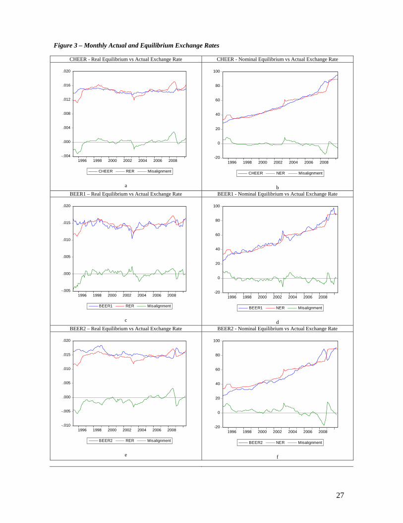
Figure 3a & b shows the SR real and nominal equilibrium exchange rate (CHEER) vis-à-vis the

respective actual exchange rate for the period being investigated. The results demonstrates that in

the period 1995 to mid 1996, the Jamaican dollar was severely undervalued for which a speedy

correction was made by the start of 1997. In the 2003 foreign exchange instability the JMD

became undervalued on account of market psychology from uncertainty. The resulting

disequilibrium gradually dissipated over the next two year. Evidence of SR disequilibrium was

observed from late 2007 during a period when oil prices begun climbing to historical highs. Since

August 2008, a month after Oil prices began falling, the foreign exchange rate went into a period

of expanded overvaluation. A significant depreciation resulted towards the end of 2008 to bring

exchange rate back to the equilibrium path.

BEER Model Results

The BEER model was estimated using equation 9. All variables were stationary in the first

difference satisfying the necessary condition for cointegration. A simple regression resulted in

approximately 35% of the variation in the RER being explained by the fundamental variables. Of

the five (5) variables, only three (3) were significant at the 5% critical level. However, including

26

constant and dummy variables resulted in over 82% of explained variation with all variables

significant at the 5% and 1% critical level. Additionally, the Jarque Bera null of no normality was

strongly rejected for the residual.

Lag length tests was based on the FPE, AIC, SC and HQ filters all recommended the nth lag of

two (2). The Johansen trace and maximum eigen value tests were then conducted to determine

the number of cointegrating vectors. The results show that there was no more than 1 cointegrating

vector at (n-1) lags. With proof of cointegration, the VECM methodology was estimated on a

single lag (n-1), accounting for one (1) cointegrating vector and no trend in the cointegrating

equation. The results show that, all variables except for Jamaica’s Terms of Trade (TOT) and Net

Foreign Asset (NFA) had the correct sign. These two variables however, were both insignificant

at the 5% and 10% critical level (see Table B in Appendix). The cointegrating coefficient (-0.06)

was significant at both the 5% and 1% critical level and appropriately signed (see Table B in

appendix). The speed of adjustment is estimated with a half-life of 13 months. The resulting

residual proved to be a unit root in levels with no significant constant or trend which supports the

notion that all information has been captured. The evidence suggest that there are no significant

explanatory power of the theoretically recommended TOT and NFA in explaining variations in

the bilateral exchange rate between Jamaica and the USA. Both fundamentals were insignificant

and inappropriately signed (see Table B in Appendix).

Among the factors that proved theoretically consistent and significant were the productivity

indicator proxied by (TNTD) which supports the Balassa Samuelson effect where an increase in

productivity will enhance competitiveness while appreciating the domestic currency.

Additionally, the differential between domestic and foreign debt (NGDD) strongly supports the

notion that increasing domestic debt will result in a depreciation of the domestic currency vis-à-

vis its US counterpart. The real interest rate differential (RIRD) significantly reflects the expected

UIP relationship between the domestic and foreign interest rate. The results show that when

Jamaica’s interest rates are relatively higher than US interest rates, the domestic dollar

depreciates to cancel the arbitrage that emerges.

27

Figure 3 – Monthly Actual and Equilibrium Exchange Rates

CHEER - Real Equilibrium vs Actual Exchange Rate CHEER - Nominal Equilibrium vs Actual Exchange Rate

-.004

.000

.004

.008

.012

.016

.020

1996 1998 2000 2002 2004 2006 2008

CHEER RER Misalignment

a

-20

0

20

40

60

80

100

1996 1998 2000 2002 2004 2006 2008

CHEER NER Misalignment

b

BEER1 – Real Equilibrium vs Actual Exchange Rate BEER1 - Nominal Equilibrium vs Actual Exchange Rate

-.005

.000

.005

.010

.015

.020

1996 1998 2000 2002 2004 2006 2008

BEER1 RER Misalignment

c

-20

0

20

40

60

80

100

1996 1998 2000 2002 2004 2006 2008

BEER1 NER Misalignment

d BEER2 – Real Equilibrium vs Actual Exchange Rate BEER2 - Nominal Equilibrium vs Actual Exchange Rate

-.010

-.005

.000

.005

.010

.015

.020

1996 1998 2000 2002 2004 2006 2008

BEER2 RER Misalignment

e

-20

0

20

40

60

80

100

1996 1998 2000 2002 2004 2006 2008

BEER2 NER Misalignment

f

28

PEER1 - Real Equilibrium vs Actual Exchange Rate PEER1 - Nominal Equilibrium vs Actual Exchange Rate

-.004

-.002

.000

.002

.004

.006

.008

.010

1996 1998 2000 2002 2004 2006 2008

PEER RER Misalignment

g

-20

0

20

40

60

80

100

1996 1998 2000 2002 2004 2006 2008

PEER NER Misalignment

h

PEER2 - Real Equilibrium vs Actual Exchange Rate PEER2 - Nominal Equilibrium vs Actual Exchange Rate

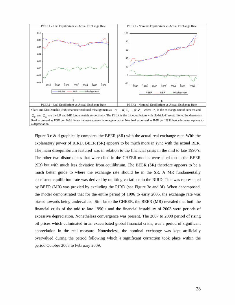
Clark and MacDonald (1998) characterized total misalignment as ttt ZZq 2211 ββ ′−′− where tq is the exchange rate of concern and

tZ1 and

tZ 2 are the LR and MR fundamentals respectively. The PEER is the LR equilibrium with Hodrick-Prescott filtered fundamentals

Real expressed as USD per JA$1 hence increase equates to an appreciation. Nominal expressed as JMD per US$1 hence increase equates to a depreciation

Figure 3.c & d graphically compares the BEER (SR) with the actual real exchange rate. With the

explanatory power of RIRD, BEER (SR) appears to be much more in sync with the actual RER.

The main disequilibrium featured was in relation to the financial crisis in the mid to late 1990’s.

The other two disturbances that were cited in the CHEER models were cited too in the BEER

(SR) but with much less deviation from equilibrium. The BEER (SR) therefore appears to be a

much better guide to where the exchange rate should be in the SR. A MR fundamentally

consistent equilibrium rate was derived by omitting variations in the RIRD. This was represented

by BEER (MR) was proxied by excluding the RIRD (see Figure 3e and 3f). When decomposed,

the model demonstrated that for the entire period of 1996 to early 2005, the exchange rate was

biased towards being undervalued. Similar to the CHEER, the BEER (MR) revealed that both the

financial crisis of the mid to late 1990’s and the financial instability of 2003 were periods of

excessive depreciation. Nonetheless convergence was present. The 2007 to 2008 period of rising

oil prices which culminated in an exacerbated global financial crisis, was a period of significant

appreciation in the real measure. Nonetheless, the nominal exchange was kept artificially

overvalued during the period following which a significant correction took place within the

period October 2008 to February 2009.

29

PEER Model Results

The PEER model was estimated using equation 11. The parameters are the same as those

specified within the BEER model. It was not deemed necessary to calculate two PEER since the

cyclical components are believed to be filtered out in the HPF transformation. The PEER

revealed that the extended undervaluation relating to the financial crisis of the 1990’s and the

overvaluation leading up to the 2008 global financial crisis were both distinctive periods of

disequilibrium. The model demonstrates, however, that the instability 2003 instability was more

inline with fundamentals. The trends demonstrate that prior to the 2003 exchange rate spike; the

real exchange rate deviated from LR equilibrium following which a corrected was made with the

2003 spike. The gradual move away from equilibrium prior to 2003 was not a distinctive feature

of the SR and MR models. Rather, in both SR and MR models, the spike appeared to be a shift

away from equilibrium whereas in the LR model, the spike appeared to be a correction. This

suggests that effectively monitoring deviations from LR equilibrium may provide invaluable

information about potential instability in the foreign exchange market.

8. COMPETITIVENESS By determining the equilibrium exchange rate, periods of disequilibrium can be more clearly

identified. It is perceived that extended periods of disequilibrium may result in suboptimal levels

of competitiveness. The paper therefore seeks to access the effects of disequilibrium on Jamaica’s

level of competitiveness. The measures of competitiveness adopted for this purpose include the

REER, ULC, TNT, and TBT. Changes in these measures of competitiveness are matched against

the computed misalignment for the CHEER, BEER1, BEER2 and PEER (see Figure 3 A,B,C and

D in the Appendix). The key relationships between disequilibrium and competitiveness over the

three (3) distinctive time periods of disequilibrium are presented below.

Financial Sector Crisis (Mid to Late 1990’s)

During this period, the CHEER and PEER reflected a marginal overvaluation while BEER2

reflected an undervaluation. The REER suggested a decline in competitiveness at the peak of

disequilibrium but reflected improved competitiveness as the misalignment converged to

equilibrium (see Figure 3A in appendix). During the Financial Crisis of the late 1990’s, the ULC

in Jamaica was declining at a significant rate (see figure 3B in appendix). At the same time the

US ULC was increasing by similar magnitude. This period was therefore characterized by

declining productivity as more was being paid in wages to generate a unit of output. As the

30

misalignment dissipated, the rate of productivity deterioration showed though worsening

considerably again in late 2001. At this point the rate of increase in US labour productivity also

slowed considerably in conjunction with the 2001 September 11 terrorist attacks. The ratio of

tradables to non-tradables showed relatively little variation in competitiveness in the period.

Foreign Currency Market Instability (2003)

In this period the CHEER and BEER2 reflected a significant spike that indicated a shift towards

an undervaluation of the JMD vis-à-vis the USD. The BEER1 model, contrary to the other

models, reflected a sharp overvaluation that was immediately followed by a large undervaluation

(see Figure 3A in appendix). During this period the REER reflected an increase in

competitiveness signaled by a significant depreciation. At this point Jamaica’s ULC switched

from a consistent deterioration to no change in competitiveness. The TNT indicator of

competitiveness reflected no significant change in competitiveness that was demonstrated by

relatively stable TNT. The TBT, similar to the REER and ULC during this period, reflected a

notable improvement in competitiveness as this was the only period during which there was as

substantial bias towards exports. This period of a relatively undervalued domestic currency

reflected a general improvement in competitiveness. Nonetheless, as the instability of 2003

corrects towards the various representations of equilibrium, the level of competitiveness

continued deteriorate.

Global Economic & Financial Crisis (2008)

During this period all four measures of misalignment reflected a strong and persistent shift away

from equilibrium beginning in mid 2007 in favour of an overvalued Jamaican dollar (see figure 3

in appendix). By mid 2008 continuing onwards, a sharp correction was evident in both the SR

CHEER and LR PEER models. The BEER1 and BEER2 however, reflected a strong shift to the

over side into a period of strong undervaluation. The two phases were strongly correlated to the

significant hike in crude oil prices leading up to mid 2008 that experienced a significant

correction following this period (phase 2). In the first phase of mounting overvaluation, the

REER reflected a consistent deterioration in the level of competitiveness. The second phase

where SR and LR exchange rates corrected, but for which MR undervaluation was signaled, the

REER sharply switched to a strong improvement in Jamaica’s level of competitiveness. In the

first phase of an expanding overvaluation of the Jamaican dollar, domestic ULC worsened while

US ULC also deteriorated. Both trends suggested a relatively stable to declining levels of

competitiveness in Jamaica. In the second phase however, domestic ULC reverted to comparable

31

levels prior to phase one of the 2008 Global financial crisis. Nonetheless, the ULC of the US

continued to descend into the negative bands reflecting a net relative improvement in Jamaica’s

level of competitiveness. This is consistent with the REER measures of competitiveness during

this period.

Similar to the REER and ULC indicators, the TNT ratio captured a falloff in competitiveness in

the first phase of expanding overvaluation. The trend, however, persisted into the second phase

where an aligned currency by SR and LR models but undervalued by MR models was matched

against a period of deteriorating levels of competitiveness or productivity as signaled by the TNT

indicator. The TBT reflected continued deterioration in the terms of trade throughout the enter

period of the Global financial crisis. This indicated that there remained a bias towards an

expanding deterioration in the trade balance which captures persistent levels of declining

competitiveness. Therefore TBT is consistent with TNT in both phases but inconsistent with the

REER and ULC second phase indication of competitiveness.

9. CONCLUSION

This paper set out to determine the equilibrium exchange rate for Jamaica over three distinctive

time horizons (SR, MR, & LR). A fundamentals based approach was embraced in modeling the

dynamics of mean reverting tendencies as implied by the theories of PPP and UIP. With the use

cointegrating techniques, proof of mean reversion was confirmed in the models presented. Error

Correction coefficients were all significant reflecting reasonable speeds of adjustment with a half

life ranging from 6 to 13 months for SR to MR models respectively.

The SR model demonstrated that variations to the Jamaican price level are not met with an

appropriate adjustment in the exchange rate that will ensure PPP. This was however evidenced in

changes in the US price index. Both variables were statistically significant. The model also

demonstrated that variation in the Jamaica’s interest rate is not met with full adjustment in the

exchange rate expected to eliminate any arbitrage between the two currencies, thus violating the

UIP condition. This was however statistically insignificant. The US interest rate was however

both statistically significant and demonstrated an approximate unitary adjustment in exchange

rate to eliminate arbitrage between yields on currency holdings. The strong reliance of Jamaica

on imported raw materials and a less efficient local foreign currency market may be the

underlying factors contributing to these results.

32

The MR and LR models reflected expected signs for all variables except TOT and NFA. Both

variables however, were statistically insignificant. In summary, the Balassa Samuelson theory

was confirmed demonstrating that the exchange rate will appreciate when productivity increases.

This was also supported by trends in the TNT productivity measure of competitiveness which

showed deterioration in competitiveness as productivity levels declined in the second phase of the

global financial crisis. Also the negative correlation between exchange rate and the risk premium

imposed by government debt was significant. Hence, increasing the domestic debt relative to

foreign debt will lead to a general depreciation of the domestic currency. The interest rate

differential was also significant with a negative sign suggesting than increases in the Jamaican

interest rate relative to the US interest rate will generate an increase in the demand and hence

appreciation of the domestic currency.

The measure of competitiveness displayed conflicting results in the financial sector crisis of the

late 1990’s due to variations in the equilibrium models. The 2003 financial sector instability and

the 2008 Global financial crisis reflected clear signals that an undervalued currency resulted in

increased levels of competitiveness. The productivity and trade flow measures of competitiveness

(TNT & TBT) however conflicted with the REER and ULC measures of competitiveness in the

second stage of the Global financial crisis. In this case, persistent decline in productivity resulted

in periods of undervaluation and was accompanied by continued deterioration in the trade

balance.

All models except for BEER1 showed visual signs of gradual correction of exchange rates

following a deviation from equilibrium. Where as the SR models suggested a sharp shift from

equilibrium in the 2003 foreign currency market instability, the LR model featured this as a

correction to deviations from the LR norm. This suggests that monitoring the LR model will

better aid in spotting potential disruption in the foreign currency markets that may be attributed to

fundamental based misalignments.

33

10. BIBLIOGRAPHY Atkins, Fiona, 2000, “Revisiting the Exchange Rate Debate: The Jamaican Experience”, Journal of International Development, vol.12, pp.121-131. Clark, Peter, and Ronald MacDonald, (1998), “Exchange Rates and Economic Fundamentals: A Methodological Comparison of BEERs and FEERs”, IMF, IMF Working Papers, WP/18/67. Driver, L, Rebecca and Peter F. Westaway, 2004, “Concepts of equilibrium exchange rates”,. Bank of England, Working Paper no. 248. Francis, A., 1998, “Is the Jamaican Dollar Overvalued?”, Social and Economic Studies, Vol.47, Issue 4, pp.29-45. Franklin, Famalia and Rohan Longmore, 2008, “Price-Setting Behaviour in the Jamaican Foreign Exchange Makret”, Bank of Jamaica. Franklin, Tamalia and Rohan Longmore, 2008, “Pric-Setting Behaviour in the Jamaican Foreign Exchange Market”, Journal Of Economic Literature Henry, Chandar, 2001, “Measuring Competitiveness in the Jamaican Economy”, Bank of Jamaica (BOJ) Working Papers, (October) MacDonald, Ronald, and Mark Taylor, (1992), “Exchange Rate Economics: A Survey”, IMF, IMF Staff Papers, Vol. 39, No. 1 (March ) Moura, M, Adauto Lima, and Rodrigo Mendonca, (2008), “Exchange Rate and Fundamentals: The Case of Brazil”, IBMEC Working Paper, WPE-66-2008. Paiva, Claudio, (2001), “Competitiveness and the Equilibrium Exchange Rate in Costa Rica”, IMF, IMF Working Papers, WP/01/23 (February) Pineda, Emilio, Paul A. Cashin and Yan Sun, 2009, “Assessing Echange Rate Competitiveness in the Eastern Caribbean Currency Union”, IMF, Working Paper no. 09/78. Williams, Pierre, 2008, “Estimating Jamaica’s Real Equilibrium Exchange Rate”, Bank of Jamaica (BOJ) Working Papers. Dockery, Everton, and Karl Taylor, (2008), “On the Validity of Long-Run Purchasing Power Parity: A look at Two Selected Caribbean Economies Exchange Rate”, Journal of Money, Investment and Banking, Issue 1 (2008). Bayoumi, Tamim, Peter Clark, Steve Symansky, and Mark Taylor (1994), “Robustness of Equilibrium Exchange Rate Calculations to Alternative Assumptions and Methodologies”, IMF, IMF Working Papers, WP/94/17 (February) Artis, Michael J., and Mark P. Taylor, (1993), “DEER Hunting: Misalignment, Debt Accumulation and Desired Equilibrium Exchange Rates”, IMF, IMF Working Papers, WP/93/48, (June)

34

Melecky, Martin, Lubos Komarek (2005), “Behavioural equilibrium exchange rate estimates and implied exchange rate adjustments for ten countries”, Transition Studies Review, 14 (1), pp. 105-121, 2007 MacDonald, Ronald, Preethike Dias (2007), “The Behavioral Equilibrium Exchange Rate of the Czech Koruna”, University of Glasgow and Peterson Institute of International Economics, Washington DC. MacDonald, Roland, and Ian W. Marsh (1997), “On Fundamentals and Exchange Rates: A Casselian Perspective”, The MIT Press, The Review of Economics and Statistics, Vol 79, No.4 (November). McFarlane, Lavern (2003), “The UIP and Time Varying Risk Premium: An Application to the Jamaican Bond Market”, Bank of Jamaica, Working Paper, November 2003. Maeso-Fernandez, Francisco, Chiara Osbat, Bernd Schnatz, (2001), “Determinants of the Euro Real Effective Exchange Rate: A BEER/PEER Approach”, European Central Bank, Working Paper No. 85, November 2001. Henry, Henry, Rohan Longmore, (2001), “Current Account Dynamics and The Real Effective Exchange Rate: The Jamaican Experience”, Bank of Jamaica, Working Paper, March 2003. Isard, Peter, and Hamid Faruqee et.al (1998), “Exchange Rate Assessment: Extensions of the Macroeconomic Balance Approach”, International Monetary Fund (IMF), Occasional Paper (167). Marsh, Ian, and Stephen Tokarick (1994), “Competitiveness Indicators: A Theoretical and Empirical Assessment”, International Monetary Fund, Working Paper (WP/94/29)

35

11. APPENDIX

Table A - Unit Root Tests for Monthly Fundamental Variables

Variables ADF PP LRER levels -2.680 [c]* -2.605 [c]* 1st diff -8.381 *** -8.489 *** LPRI_ja levels -2.527 [c,t] -0.503 [c] 1st diff -6.438 [c]*** -6.438 [c]*** LPRI_us levels -3.313 [c,t]* -3.148 [c,t]* 1st diff -8.758 [c]*** -6.850 [c]*** INT_ja levels -3.170 [c,t]* -0.818 1st diff -9.508 *** -9.514 *** INT_us levels -1.495 -1.394 1st diff -5.280 *** -11.052 *** LNFA levels -2.974 [c]** -2.856 [c]* 1st diff -12.864 [c,t]*** -12.864 [c,t]*** RIRD levels -4.111 [c,t]*** -2.782 [c]* 1st diff -8.989 *** -9.214 *** LNGDD levels -3.493 *** -3.784 *** 1st diff -15.950 [c,t]*** -15.927 [c,t]*** LTNTD levels -3.160 [c]** -3.191 [c]** 1st diff -9.183 [c,t]*** -9.398 [c,t]*** LTOT levels -2.627 [c,t] -2.971 [c,t] 1st diff -11.764 *** -11.764 ***

Significance is indicated as *** at 1%, ** at 5%, and * at 10%

Table B - Estimation Results for BEER, PEER, FEER and CHEER Models

Variable Sign SR Model SR Model MR Model MR Model NAME [+/-] CHEER CHEER(2) BEER (1) FEER

Dependent LNER LNER LRER PRI_JA -0.4845 -0.2810 ---

(-4.077) (-2.040) PRI_US -0.9558 -1.9620 ---

(-2.057) (-3.787) INT_JA 0.0441 --- ---

(0.435) INT_US 1.0122 --- ---

(2.7687) LTNTD --- --- 0.2241

[+] (5.584) LNGDD --- --- -0.0989

[+/-] (-2.455) LTOT --- --- -0.0325

[-] (-0.296) RIRD --- -0.4512 -1.1574

[-] (3.787) (-6.823) LNFA --- --- -0.030268

[+] (--0.0160) CONSTANT 2.3682 2.3682 4.2058

COINT Coeff [-] -0.1501 -0.1501 -0.0576

[-4.941] [-4.941] (-2.867) R-Squared 0.380 0.380

Adj-Rsquared 0.345 DW Statistic

Jarque-Bera (Prob) LM Test (2)

ADF (Unit Root) -13.481 *** -7.414116 *** -7.414116 *** Significance is indicated as *** at 1%, ** at 5%, and * at 10% ; FEER (1) uses specification from Plaudio Paiva (IMF-

Working Paper). [e] refers to expected sign and[r] pertains to the resulting sign from estimation.

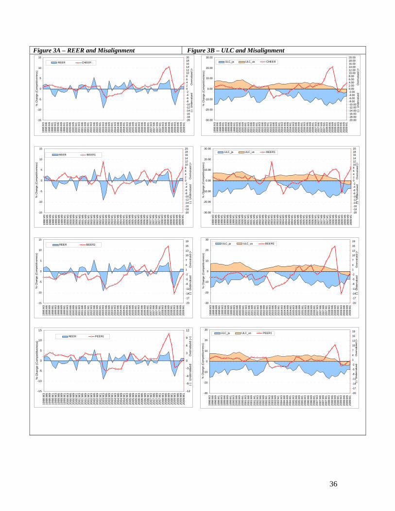
36

Figure 3A – REER and Misalignment Figure 3B – ULC and Misalignment

-15

-10

-5

0

5

10

15

1998

:M3

1998

:M6

1998

:M9

1998

:M1

1999

:M3

1999

:M6

1999

:M9

1999

:M1

2000

:M3

2000

:M6

2000

:M9

2000

:M1

2001

:M3

2001

:M6

2001

:M9

2001

:M1

2002

:M3

2002

:M6

2002

:M9

2002

:M1

2003

:M3

2003

:M6

2003

:M9

2003

:M1

2004

:M3

2004

:M6

2004

:M9

2004

:M1

2005

:M3

2005

:M6

2005

:M9

2005

:M1

2006

:M3

2006

:M6

2006

:M9

2006

:M1

2007

:M3

2007

:M6

2007

:M9

2007

:M1

2008

:M3

2008

:M6

2008

:M9

2008

:M1

2009

:M3

2009

:M6

2009

:M9

2009

:M1

% C

hang

e (C

ompe

titiv

enes

s)

-20-18-16-14-12-10-8-6-4-202468101214161820

(-)

Und

erva

lued

O

verv

alue

d (+

REER CHEER

-15

-10

-5

0

5

10

15

1998

:M3

1998

:M6

1998

:M9

1998

:M1

1999

:M3

1999

:M6

1999

:M9

1999

:M1

2000

:M3

2000

:M6

2000

:M9

2000

:M1

2001

:M3

2001

:M6

2001

:M9

2001

:M1

2002

:M3

2002

:M6

2002

:M9

2002

:M1

2003

:M3

2003

:M6

2003

:M9

2003

:M1

2004

:M3

2004

:M6

2004

:M9

2004

:M1

2005

:M3

2005

:M6

2005

:M9

2005

:M1

2006

:M3

2006

:M6

2006

:M9

2006

:M1

2007

:M3

2007

:M6

2007

:M9

2007

:M1

2008

:M3

2008

:M6

2008

:M9

2008

:M1

2009

:M3

2009

:M6

2009

:M9

2009

:M1

% C

hang

e (C

ompe

titiv

enes

s)

-20-18-16-14-12-10-8-6-4-202468101214161820

(-)

Und

erva

lued

Ove

rval

ued

(+

REER BEER1

-15

-10

-5

0

5

10

15

1998

:M3

1998

:M6

1998

:M9

1998

:M1

1999

:M3

1999

:M6

1999

:M9

1999

:M1

2000

:M3

2000

:M6

2000

:M9

2000

:M1

2001

:M3

2001

:M6

2001

:M9

2001

:M1

2002

:M3

2002

:M6

2002

:M9

2002

:M1

2003

:M3

2003

:M6

2003

:M9

2003

:M1

2004

:M3

2004

:M6

2004

:M9

2004

:M1

2005

:M3

2005

:M6

2005

:M9

2005

:M1

2006

:M3

2006

:M6

2006

:M9

2006

:M1

2007

:M3

2007

:M6

2007

:M9

2007

:M1

2008

:M3

2008

:M6

2008

:M9

2008

:M1

2009

:M3

2009

:M6

2009

:M9

2009

:M1

% C

hang

e (C

ompe

titiv

enes

s)

-20

-17

-14

-11

-8

-5

-2

1

4

7

10

13

16

19

(-)

Und

erva

lued

O

verv

alue

d (+

REER BEER2

-15

-10

-5

0

5

10

15

1998

:M3

1998

:M6

1998

:M9

1998

:M1

1999

:M3

1999

:M6

1999

:M9

1999

:M1

2000

:M3

2000

:M6

2000

:M9

2000

:M1

2001

:M3

2001

:M6

2001

:M9

2001

:M1

2002

:M3

2002

:M6

2002

:M9

2002

:M1

2003

:M3

2003

:M6

2003

:M9

2003

:M1

2004

:M3

2004

:M6

2004

:M9

2004

:M1

2005

:M3

2005

:M6

2005

:M9

2005

:M1

2006

:M3

2006

:M6

2006

:M9

2006

:M1

2007

:M3

2007

:M6

2007

:M9

2007

:M1

2008

:M3

2008

:M6

2008

:M9

2008

:M1

2009

:M3

2009

:M6

2009

:M9

2009

:M1

% C

hang

e (C

ompe

titiv

enes

s)

-12

-9

-6

-3

0

3

6

9

12

(-)

Und

erva

lued

O

verv

alue

d (+

)REER PEER1

-30.00

-20.00

-10.00

0.00

10.00

20.00

30.00

1998

:M3

1998

:M6

1998

:M9

1998

:M1

1999

:M3

1999

:M6

1999

:M9

1999

:M1

2000

:M3

2000

:M6

2000

:M9

2000

:M1

2001

:M3

2001

:M6

2001

:M9

2001

:M1

2002

:M3

2002

:M6

2002

:M9

2002

:M1

2003

:M3

2003

:M6

2003

:M9

2003

:M1

2004

:M3

2004

:M6

2004

:M9

2004

:M1

2005

:M3

2005

:M6

2005

:M9

2005

:M1

2006

:M3

2006

:M6

2006

:M9

2006

:M1

2007

:M3

2007

:M6

2007

:M9

2007

:M1

2008

:M3

2008

:M6

2008

:M9

2008

:M1

2009

:M3

2009

:M6

2009

:M9

2009

:M1

% C

hang

e (C

ompe

titiv

enes

s)

-20.00-18.00-16.00-14.00-12.00-10.00-8.00-6.00-4.00-2.000.002.004.006.008.0010.0012.0014.0016.0018.0020.00

(-)

Und

erva

lued

O

verv

alue

d (+

ULC_ja ULC_us CHEER

-30.00

-20.00

-10.00

0.00

10.00

20.00

30.00

1998

:M3

1998

:M6

1998

:M9

1998

:M1

1999

:M3

1999

:M6

1999

:M9

1999

:M1

2000

:M3

2000

:M6

2000

:M9

2000

:M1

2001

:M3

2001

:M6

2001

:M9

2001

:M1

2002

:M3

2002

:M6

2002

:M9

2002

:M1

2003

:M3

2003

:M6

2003

:M9

2003

:M1

2004

:M3

2004

:M6

2004

:M9

2004

:M1

2005

:M3

2005

:M6

2005

:M9

2005

:M1

2006

:M3

2006

:M6

2006

:M9

2006

:M1

2007

:M3

2007

:M6

2007

:M9

2007

:M1

2008

:M3

2008

:M6

2008

:M9

2008

:M1

2009

:M3

2009

:M6

2009

:M9

2009

:M1

% C

hang

e (C

ompe

titiv

enes

s)

-20-18-16-14-12-10-8-6-4-202468101214161820

(-)

Und

erva

lued

Ove

rval

ued

(+

ULC_ja ULC_us BEER1

-30

-20

-10

0

10

20

30

1998

:M3

1998

:M6

1998

:M9

1998

:M1

1999

:M3

1999

:M6

1999

:M9

1999

:M1

2000

:M3

2000

:M6

2000

:M9

2000

:M1

2001

:M3

2001

:M6

2001

:M9

2001

:M1

2002

:M3

2002

:M6

2002

:M9

2002

:M1

2003

:M3

2003

:M6

2003

:M9

2003

:M1

2004

:M3

2004

:M6

2004

:M9

2004

:M1

2005

:M3

2005

:M6

2005

:M9

2005

:M1

2006

:M3

2006

:M6

2006

:M9

2006

:M1

2007

:M3

2007

:M6

2007

:M9

2007

:M1

2008

:M3

2008

:M6

2008

:M9

2008

:M1

2009

:M3

2009

:M6

2009

:M9

2009

:M1

% C

hang

e (C

ompe

titiv

enes

s)

-20

-17

-14

-11

-8

-5

-2

1

4

7

10

13

16

19

(-)

Und

erva

lued

O

verv

alue

d (+

ULC_ja ULC_us BEER2

-30

-20

-10

0

10

20

30

1998

:M3

1998

:M6

1998

:M9

1998

:M1

1999

:M3

1999

:M6

1999

:M9

1999

:M1

2000

:M3

2000

:M6

2000

:M9

2000

:M1

2001

:M3

2001

:M6

2001

:M9

2001

:M1

2002

:M3

2002

:M6

2002

:M9

2002

:M1

2003

:M3

2003

:M6

2003

:M9

2003

:M1

2004

:M3

2004

:M6

2004

:M9

2004

:M1

2005

:M3

2005

:M6

2005

:M9

2005

:M1

2006

:M3

2006

:M6

2006

:M9

2006

:M1

2007

:M3

2007

:M6

2007

:M9

2007

:M1

2008

:M3

2008

:M6

2008

:M9

2008

:M1

2009

:M3

2009

:M6

2009

:M9

2009

:M1

% C

hang

e (C

ompe

titiv

enes

s)

-20

-17

-14

-11

-8

-5

-2

1

4

7

10

13

16

19

(-)

Und

erva

lued

O

verv

alue

d (+

ULC_ja ULC_us PEER1

37

Figure 3C – TNT and Misalignment Figure 3D – TBT and Misalignment

-10

-8

-6

-4

-2

0

2

4

6

8

10

1998

:M3

1998

:M6

1998

:M9

1998

:M1

1999

:M3

1999

:M6

1999

:M9

1999

:M1

2000

:M3

2000

:M6

2000

:M9

2000

:M1

2001

:M3

2001

:M6

2001

:M9

2001

:M1

2002

:M3

2002

:M6

2002

:M9

2002

:M1

2003

:M3

2003

:M6

2003

:M9

2003

:M1

2004

:M3

2004

:M6

2004

:M9

2004

:M1

2005

:M3

2005

:M6

2005

:M9

2005

:M1

2006

:M3

2006

:M6

2006

:M9

2006

:M1

2007

:M3

2007

:M6

2007

:M9

2007

:M1

2008

:M3

2008

:M6

2008

:M9

2008

:M1

2009

:M3

2009

:M6

2009

:M9

2009

:M1

% C

hang

e (C

ompe

titiv

enes

s)

-20-18-16-14-12-10-8-6-4-202468101214161820

(-)

Und

erva

lued

O

verv

alue

d (+

TNT CHEER

-10

-8

-6

-4

-2

0

2

4

6

8

10

1998

:M3

1998

:M6

1998

:M9

1998

:M1

1999

:M3

1999

:M6

1999

:M9

1999

:M1

2000

:M3

2000

:M6

2000

:M9

2000

:M1

2001

:M3

2001

:M6

2001

:M9

2001

:M1

2002

:M3

2002

:M6

2002

:M9

2002

:M1

2003

:M3

2003

:M6

2003

:M9

2003

:M1

2004

:M3

2004

:M6

2004

:M9

2004

:M1

2005

:M3

2005

:M6

2005

:M9

2005

:M1

2006

:M3

2006

:M6

2006

:M9

2006

:M1

2007

:M3

2007

:M6

2007

:M9

2007

:M1

2008

:M3

2008

:M6

2008

:M9

2008

:M1

2009

:M3

2009

:M6

2009

:M9

2009

:M1

% C

hang

e (C

ompe

titiv

enes

s)

-20-18-16-14-12-10-8-6-4-202468101214161820

(-)

Und

erva

lued

Ove

rval

ued

(+

TNT BEER1

-10

-8

-6

-4

-2

0

2

4

6

8

10

1998

:M3

1998

:M6

1998

:M9

1998

:M1

1999

:M3

1999

:M6

1999

:M9

1999

:M1

2000

:M3

2000

:M6

2000

:M9

2000

:M1

2001

:M3

2001

:M6

2001

:M9

2001

:M1

2002

:M3

2002

:M6

2002

:M9

2002

:M1

2003

:M3

2003

:M6

2003

:M9

2003

:M1

2004

:M3

2004

:M6

2004

:M9

2004

:M1

2005

:M3

2005

:M6

2005

:M9

2005

:M1

2006

:M3

2006

:M6

2006

:M9

2006

:M1

2007

:M3

2007

:M6

2007

:M9

2007

:M1

2008

:M3

2008

:M6

2008

:M9

2008

:M1

2009

:M3

2009

:M6

2009

:M9

2009

:M1

% C

hang

e (C

ompe

titiv

enes

s)

-20

-17

-14

-11

-8

-5

-2

1

4

7

10

13

16

19

(-)

Und

erva

lued

O

verv

alue

d (+

TNT BEER2

-10

-8

-6

-4

-2

0

2

4

6

8

10

1998

:M3

1998

:M6

1998

:M9

1998

:M1

1999

:M3

1999

:M6

1999

:M9

1999

:M1

2000

:M3

2000

:M6

2000

:M9

2000

:M1

2001

:M3

2001

:M6

2001

:M9

2001

:M1

2002

:M3

2002

:M6

2002

:M9

2002

:M1

2003

:M3

2003

:M6

2003

:M9

2003

:M1

2004

:M3

2004

:M6

2004

:M9

2004

:M1

2005

:M3

2005

:M6

2005

:M9

2005

:M1

2006

:M3

2006

:M6

2006

:M9

2006

:M1

2007

:M3

2007

:M6

2007

:M9

2007

:M1

2008

:M3

2008

:M6

2008

:M9

2008

:M1

2009

:M3

2009

:M6

2009

:M9

2009

:M1

% C

hang

e (C

ompe

titiv

enes

s)

-20

-17

-14

-11

-8

-5

-2

1

4

7

10

13

16

19

(-)

Und

erva

lued

O

verv

alue

d (+

TNT PEER1

-30

-20

-10

0

10

20

30

1998

:M3

1998

:M6

1998

:M9

1998

:M1

1999

:M3

1999

:M6

1999

:M9

1999

:M1

2000

:M3

2000

:M6

2000

:M9

2000

:M1

2001

:M3

2001

:M6

2001

:M9

2001

:M1

2002

:M3

2002

:M6

2002

:M9

2002

:M1

2003

:M3

2003

:M6

2003

:M9

2003

:M1

2004

:M3

2004

:M6

2004

:M9

2004

:M1

2005

:M3

2005

:M6

2005

:M9

2005

:M1

2006

:M3

2006

:M6

2006

:M9

2006

:M1

2007

:M3

2007

:M6

2007

:M9

2007

:M1

2008

:M3

2008

:M6

2008

:M9

2008

:M1

2009

:M3

2009

:M6

2009

:M9

2009

:M1

% C

hang

e (C

ompe

titiv

enes

s)

-20-18-16-14-12-10-8-6-4-202468101214161820

(-)

Und

erva

lued

O

verv

alue

d (+

TBT CHEER

-30

-20

-10

0

10

20

30

1998

:M3

1998

:M6

1998

:M9

1998

:M1

1999

:M3

1999

:M6

1999

:M9

1999

:M1

2000

:M3

2000

:M6

2000

:M9

2000

:M1

2001

:M3

2001

:M6

2001

:M9

2001

:M1

2002

:M3

2002

:M6

2002

:M9

2002

:M1

2003

:M3

2003

:M6

2003

:M9

2003

:M1

2004

:M3

2004

:M6

2004

:M9

2004

:M1

2005

:M3

2005

:M6

2005

:M9

2005

:M1

2006

:M3

2006

:M6

2006

:M9

2006

:M1

2007

:M3

2007

:M6

2007

:M9

2007

:M1

2008

:M3

2008

:M6

2008

:M9

2008

:M1

2009

:M3

2009

:M6

2009

:M9

2009

:M1

% C

hang

e (C

ompe

titiv

enes

s)

-20-18-16-14-12-10-8-6-4-202468101214161820

(-)

Und

erva

lued

Ove

rval

ued

(+

TBT BEER1

-30

-20

-10

0

10

20

30

1998

:M3

1998

:M6

1998

:M9

1998

:M1

1999

:M3

1999

:M6

1999

:M9

1999

:M1

2000

:M3

2000

:M6

2000

:M9

2000

:M1

2001

:M3

2001

:M6

2001

:M9

2001

:M1

2002

:M3

2002

:M6

2002

:M9

2002

:M1

2003

:M3

2003

:M6

2003

:M9

2003

:M1

2004

:M3

2004

:M6

2004

:M9

2004

:M1

2005

:M3

2005

:M6

2005

:M9

2005

:M1

2006

:M3

2006

:M6

2006

:M9

2006

:M1

2007

:M3

2007

:M6

2007

:M9

2007

:M1

2008

:M3

2008

:M6

2008

:M9

2008

:M1

2009

:M3

2009

:M6

2009

:M9

2009

:M1

% C

hang

e (C

ompe

titiv

enes

s)

-20

-17

-14

-11

-8

-5

-2

1

4

7

10

13

16

19

(-)

Und

erva

lued

O

verv

alue

d (+

TBT BEER2

-30

-20

-10

0

10

20

30

1998

:M3

1998

:M6

1998

:M9

1998

:M1

1999

:M3

1999

:M6

1999

:M9

1999

:M1

2000

:M3

2000

:M6

2000

:M9

2000

:M1

2001

:M3

2001

:M6

2001

:M9

2001

:M1

2002

:M3

2002

:M6

2002

:M9

2002

:M1

2003

:M3

2003

:M6

2003

:M9

2003

:M1

2004

:M3

2004

:M6

2004

:M9

2004

:M1

2005

:M3

2005

:M6

2005

:M9

2005

:M1

2006

:M3

2006

:M6

2006

:M9

2006

:M1

2007

:M3

2007

:M6

2007

:M9

2007

:M1

2008

:M3

2008

:M6

2008

:M9

2008

:M1

2009

:M3

2009

:M6

2009

:M9

2009

:M1

% C

hang

e (C

ompe

titiv

enes

s)

-20

-17

-14

-11

-8

-5

-2

1

4

7

10

13

16

19

(-)

Und

erva

lued

O

verv

alue

d (+

TBT PEER1