Embed Size (px)
Citation preview
Real Exchange Rate and Structural Change in a Kaldorian Balance of Payments Constrained Growth Model
Bernardo Mattos Santana *
José Luis Oreiro **
Resumo: O presente artigo tem por objetivo desenvolver um modelo Kaldoriano de
crescimento que (i) incorpore a restrição de balanço de pagamentos, eliminando assim a
inconsistência presente nos MCRBP; e (ii) estabeleça um mecanismo pelo qual o nível
da taxa real de câmbio possa afetar o crescimento de longo-prazo das economias
capitalistas. Uma inovação importante introduzida no modelo que será desenvolvido ao
longo desse artigo é a hipótese de que o coeficiente de Kaldor-Verdoorn - que capta a
sensibilidade da taxa de crescimento da produtividade do trabalho com respeito a taxa de
crescimento da produto real - depende da participação da indústria no PIB. Essa hipótese
permitirá introduzir no modelo a possibilidade de mudança estrutural, a qual é entendida
como um processo dinâmico mediante o qual a participação da indústria no produto se
altera ao longo do tempo. Dessa forma, será possível analisar as propriedades dinâmicas
do modelo tanto no caso em que a estrutura produtiva é mantida constante (caso sem
mudança estrutural), como no caso em que a mesma se altera em decorrência de algum
processo econômico (caso com mudança estrutural).
Palavras-Chave: Crescimento puxado pela demanda, câmbio real, mudança estrutural.
Abstract: The objective of the present article is to develop a Kaldorian Growth model
that (i) had a balance of payments constraint, in order to eliminate the inconsistency of
balance of payments growth models; and (ii) defines a precise mechanism by which the
level of real exchange rate can affect long-term growth. An important innovation
introduced in the model is the idea that Kaldor-Verdoorn coefficient – that measures the
sensibility of growth rate of labor productivity to output growth – depends on the share
of manufacturing output on GDP. This hypothesis allowed us to introduce the possibility
of structural change, defined as a dynamic process by which the share of manufacturing
industry on real output could change over time. In this case, it will be possible to analyze
the dynamic properties of the model either in the case where productive structure is kept
constant (case with no structural change), as in the case where it evolves over time as a
result of some economic process (case with structural change).
Key-Words: Demand-led Growth, Real Exchange Rate, Structural Change.
Jel-Code: O1, O11; O12
* Master in Economics, Universidade Federal do Rio de Janeiro (UFRJ). Economist of Banco Nacional do
Desenvolvimento Economico e Social (BNDES). E-mail: [email protected]. ** Professor at Departamento de Economia, Universidade de Brasília (UnB) and Level IB Researcher at
CNPq. E-mail: [email protected]. Website: www.joseluisoreiro.com.br.

1. Introduction
The balance of payments constrained growth model, pioneered developed by Anthony
Thirwall(1979), holds two fundamental problems. Firstly, they fully disregard the
cumulative causation mechanism, so relevant to kaldorian growth models. Indeed,
assuming constant terms of trade then productivity gains induced by economic growth
have no effect over the dynamics of the system, in a such way they become, strictly,
irrelevant. However, in this case, the system no longer has any adjustment mechanism
between aggregate supply and demand. This deficiency was observed by Palley (2002)
for whom the balance of payments constrained growth model would be inconsistent in
the extent that only in a “happy coincidence” would be possible the equality between the
growth rate compatible with the balance of payments equilibrium and natural growth rate,
i.e., the one that keeps the unemployment rate constant over the time. In this way, the
balance of payments constrained growth models are not, in general, compatible with a
balanced growth path.
Last but not least, the balance of payments constrained growth models fully neglect the
relationship between the real exchange rate and the long-term growth. Indeed, in those
models the long-term equilibrium growth rate depends on the ratio of export and import
income elasticities multiplied by rest of the world growth rate. Thus, real exchange rate
variations are assumed irrelevant to the long-term growth either because empirical
evidence shows that finding that export and import price elasticities are low, in a such
way that the impact of a real devaluation of exchange rate over the growth path of exports
and imports is low; either because the terms of trade do not show a systematic trend to
appreciation or depreciation in the long-term.
In recent years, an interesting literature has been developed about the relation between
real exchange and economic growth. The Razin and Collins (1997) seminal paper
indicated to the existence of important non-linearities in the relationship between
exchange rate misalignment - defined as a lasting deviation of the real exchange rate with
respect to some reference value, determined by the "fundamentals"- and the real output
growth in a sample of 93 developing and developed countries between 1975-1993.
Indeed, the empirical results showed that while only very large overvaluations of real
exchange rate are associated with a slower economic growth in the long term, even
moderated undervaluation of the real exchange rate have a positive effect on economic
growth. Rodrik (2008), analyzing the development strategies adopted by a group of
countries, noted that an important factor for the ignition of a process of sustained growth
of the real output is the maintenance of an undervalued and stable real exchange rate.
Similarly, Frenkel (2004) - analyzing the employment and the growth rate performance
of Argentina, Brazil, Chile and Mexico – verified that maintaining a competitive and
stable real exchange rate is the best contribution the macroeconomic policy can provide
to the long-term growth. In the Brazilian case, Oreiro, Punzo e Aráujo (2012) indicated
to the existence of a negative and statistically significant effects of exchange rate
misalignment over output growth rate in the period 1994-2007. Therefore, the absence of
a connection between the level of the real exchange rate and the long-term growth in the
context of the balance of payments constrained growth models becomes theoretically
unacceptable.
Hence, this article aims to develop a kaldorian growth model that (i) incorporates
the balance of payments constraint, eliminating the inconsistency presented on balance of

payments constrained growth models; (ii) establishes a mechanism by which the level of
the real exchange rate may affect the long-term growth of capitalist economies.
The model to be developed throughout this article incorporates some innovations
introduced by Oreiro (2009) into the structure of Kaldorian growth models, such as the
conduction of monetary policy in a Inflation Target Regime, nominal interest rate
determined by a Taylor rule, a floating exchange rate regime and imperfect capital
mobility. In contrast to the Oreiro model, however, we will assume a balance of payments
constraint in which the growth rate of international capital inflows is a positve function
of the differential between the domestic interest rate and the international interest rate
plus the country risk premium. In this context, the differential between the domestic and
international interest rates (plus the risk premium) will also determine the rate of
depreciation (or appreciation) of the nominal exchange rate.
Another important innovation introduced in the model that will be developed
throughout this article is the hypothesis that the Kaldor-Verdoorn coefficient - which
captures the sensibility of the rate of growth of labor productivity with respect to the rate
of growth of the real output - depends on the manufacturing share on output. This
hypothesis will allow to introduce into the model the possibility of structural change,
which is understood as a dynamic process by which the manufacturing share of output
changes over time. In this way, it will be possible to analyze the dynamic properties of
the model both in the case where the productive structure is kept constant (case with no
structural change), and in a situation in which it changes due to some economic process
(case with structural change).
The structural change, in its turn, will be induced by the exchange rate
misalignment, that is, by the difference between the actual value of the real exchange
rate and the level of the real exchange rate that would correspond to the "industrial
equilibrium", in other words, the exchange rate level in which domestic firms that use
state-of-art technologies are competitive in international markets (Bresser-Pereira, Oreiro
and Marconi, 2014, 2015).
In the case of an economy with no structural change, the analysis of the short-run
equilibrium solution of the model shows that the growth rate compatible with the
equilibrium of the balance of payments can be affected by changes in the medium-term
inflation target in a such way that money is non-neutral, at least in the short term. In
addition, changes in the international economic scenario in the form of variations in the
growth rate of the rest of the world´s income and / or in the international inflation rate are
transmitted to the domestic economy in the form of changes in the output growth rate and
inflation rate.
Analyzing the properties of the balanced growth path in the case of an economy
with no structural change, we find two interesting results. The first one is that the output
growth rate along this path is independent of the medium-term inflation target, so that
money is neutral in the long term. This is another surprising result given that in Kaldorian
models output growth is demand-led. The second interesting result is that inflation rate
does not converge to the medium-term target defined by the monetary authority.
The result of the monetary policy neutrality in the long run will no longer holds,
however, in the case of an economy with structural change. In this context, raising the
inflation target pursued by the Monetary Authority has the effect of inducing an increase
in the share of the manufacturing industry in GDP, since it induces a devaluation of real
exchange with respect to its industrial equilibrium level. Though this devaluation is purely
temporary, it is capable of inducing a structural change in the economy, which will
eventually increase the Kaldor-Verdoorn coefficient and, thus, the output growth rate
along the balanced growth path.
2 – Structure of the Model
Let us consider a small open economy with a free-floating exchange rate regime
and imperfect capital mobility, in which growth rate of exports and imports are given by:
�̂�𝑡 = μ(�̂�𝑡∗ − �̂�𝑡 + �̂�𝑡) + ε�̂�𝑡 (1)
�̂�𝑡 = γ(�̂�𝑡 − �̂�𝑡∗ − �̂�t) + π�̂�𝑡 (2)
In which �̂�𝑡 is the growth rate of exports (quantum) the period t, �̂�𝑡 is the growth
rate of imports (quantum) in the period t, �̂�𝑡 is the domestic rate of inflation in the period
t, �̂�𝑡∗ is the rest of the world inflation in the period t, �̂�𝑡 is the rate of depreciation of
nominal exchange in period t, �̂�𝑡 is the domestic output/income growth rate in the period
t, �̂�𝑡 is the rest of the world output/income growth rate in the period t, μ is price elasticity
of exports, γ is the price elasticity of imposrts, ε is the income elasticity of exports, π is
the income elasticity of imports.
We will assume the validity of Marshall-Lerner's condition, so that:
μ + γ > 1 (3)
Such as in Moreno-Brid’s (2003)1 model we will assume that the Balance of
Payments restriction in period t is given by:
�̂�𝑡 + �̂�𝑡∗ + �̂�𝑡 = θ1(�̂�𝑡 + �̂�𝑡 ) − θ2(�̂�𝑡 + �̂�𝑡) + (1 − θ1 + θ2)(p̂t + f̂t) (4)
In which: θ1 = px
ep∗m is the ratio between the initial value of exports and the initial
value of imports; θ2 = pr
ep∗m is the ratio between the initial value of external liability
services and the initial value of imports; �̂�𝑡 is the growth rate of services (interest and
dividends) related to the external liabilities in the period t, e f̂ is the real growth rate of
external capital flows in period t.
Two important points can be observed in this equation. The first one is that the
constraint imposed here is "deflated" in terms of value paid by imports. The second one
is that we are considering an economy with a net debt to the rest of the world, since θ2 is
a positive parameter and there is a negative signal before it.
Assuming capital mobility to be imperfect in Mundell's sense, the real rate of
growth of external capital flows will be a function of the difference between the domestic
interest rate and the international interest rate adjusted by the country risk premium. We
have :
𝑓𝑡 = ℎ(𝑖𝑡 − 𝑖𝑡∗ − 𝜌) (5)
1 This approach advances Thirlwall and Hussain (1982), since they did not take into account the role of interest payments.
In which h is the sensibility of external capital flow growth rate to the interest
differential2, 𝑖𝑡 is the domestic interest rate in the period t, 𝑖𝑡∗ international interest rate
and 𝜌 country risk premium3.
In an economy with an open capital account, the dynamics of the nominal
exchange rate, assuming a free-floating exchange rate regime, depends fundamentally on
inflows and outflows of foreign capital. Thus, we will assume that the rate of change of
the nominal exchange rate will be a (negative) function of the growth rate of the external
capital flows as in equation (6) below:
�̂�𝑡 = −𝑘𝑓𝑡 (6)
Where k is the coefficient of sensibility of the variation of nominal exchange rate
in relation to the growth rate of external capital flows4.
Regarding the determination of the domestic interest rate, we will assume that the
economy under consideration operates with an inflation targeting regime, so that the
monetary authority should deliver to society, in the medium term, an inflation rate equal
to the target �̂�𝑇. To achieve this goal, the monetary authority sets the interest rate based
on a modified version of the Taylor5 rule such as the one assumed below:
𝑖𝑡 = (𝑖𝑡∗ + 𝜌) + 𝛽(�̂�𝑡 − �̂�𝑇) (7)
In which: 𝛽 represents the degree of aversion of the monetary authority to the
deviations of the inflation rate from the medium-term inflation target.
With regard to domestic inflation rate, we will assume that it is equal to the
difference between wage inflation and the rate of growth of labor productivity6, according
to equation (8) below.
�̂�𝑡 = �̂�𝑡 − �̂�𝑡 (8)
Regarding the determination of the growth rate of labor productivity, we will
assume the existence of static and dynamics economies of scale so that the so-called
Kaldor-Verdoorn law is valid. Then, we have7:
�̂�𝑡 = 𝑐 + 𝛼𝜆𝑡−1�̂�𝑡−1 (9)
2 This parameter h reflects, among other things, the level of capital controls in the economy. Indeed, if the inflow of foreign capital is prohibited by law, as occurred during the period of the Bretton Woods agreement, then h = 0, so that the differential between domestic and external interest will have no consequence in terms of attraction or repulsion of foreign capital from the country. On the other hand, the higher the value of h, the greater the sensibility of external capital flows to the differential between internal and external interest rates and, therefore, lower will be the level of capital controls. On regard to the economics of capital controls, see Oreiro (2004). 3 Without loss of generality we will assume that the country risk premium is constant over time. 4 This parameter fundamentally reflects the density of the foreign exchange market, that is, the volume of operations that take place daily in that market. As higher the exchange market density is, the sensitivity of the nominal exchange rate to inflows and outflows of foreign capital will be the lower. 5 This is a modified version because the output (or growth) gap is absent from the equation, meaning that the monetary authority is only concerned with the deviations of inflation from the medium-term target. A specification similar to this can be found in Carlin and Soskice (2006, p.152). 6 This equation can easily be deduced from a pricing rule based on mark-up of the type: p = (1 + τ) w / q, where p is the price of the domestic product, τ is the mark-up rate -up, w is the nominal wage rate and q is the labor productivity. To arrive at equation (8) it is enough to consider that the mark-up rate is constant and that the work is the only input used in the production. 7 This approach of Kaldor-Verdoorn law is based on Botta (2009) and Gabriel, Gonzaga and Oreiro (2016)

In which 𝛼 is the the so-called Kaldor-Verdoorn coefficient, which reflects the
degree of productivity dynamism of the economy, that is, the extent in which output
growth (from the previous period) induces productivity growth (in the current period);
and 𝜆𝑡−1 is the manufacturing share on output in the period t-1. This Kaldor-Verdoorn
law approach gives relevance to the manufacturing industrial sector in the productivity
dynamics of the economy, as Kaldor believed this sector to be the “engine of growth” of
outout and productivity.
Wage inflation, in turn, depends on the rate of domestic inflation in the previous
period and the behavior of the labor market. The idea here is that nominal wages are
determined by a process of collective bargaining, in which unions seeks, in first place, to
defend the wages’ purchasing power from losses due to inflation. In this way, unions will
demand nominal wages changes to be at least equal to the inflation observed in the
previous period. However, depending on the actual situation in the labor market, unions
may demand real wage gains, that is, they may require changes of nominal wages that
surpasses, for a certain margin, the inflation observed in the previous period. This should
happen in those periods when labor demand is growing ahead of the labor supply so that
unemployment rate is decreasing consistently over time. Otherwise, unions may be forced
to accept a nominal wage changes that are lower than inflation in the previous period. In
this case, there will be a real wage loss.
So, the wage inflation determination equation is given by:
�̂�𝑡 = �̂�𝑡−1 + 𝑙𝑑,𝑡 − 𝑙𝑠,𝑡 (10) 8
In which 𝑙𝑑,𝑡 is the rate of growth of the labor demand in period t, 𝑙𝑠,𝑡 is the rate
of growth of the labor supply in period t.
The labor demand growth rate is equal to the difference between the output growth
rate and the labor productivity growth rate, as we can see in equation (11) below.
𝑙𝑑,𝑡 = �̂�𝑡 − �̂�𝑡 (11)
Finally, without loss of generality, we will assume that the rate of growth of labor
supply is constant and equal to.
𝑙𝑠,𝑡 = (12)
8 This equation is derived from a Phillips Curve with adaptive expectations, in which the increase in wages (wage inflation) will be a function of the change of unemployment in the economy and the rate of inflation
of the previous period.

2.1 – Short-term Equilibrium
The kaldorian growth model presented in the previous section is compounded by
the following equations:
�̂�𝑡 = μ(�̂�𝑡∗ − �̂�𝑡 + �̂�𝑡) + ε�̂�𝑡 (1)
�̂�𝑡 = γ(�̂�𝑡 − �̂�𝑡∗ − �̂�t) + π�̂�𝑡 (2)
�̂�𝑡 + �̂�𝑡∗ + �̂�𝑡 = θ1(�̂�𝑡 + �̂�𝑡 ) + θ2(�̂�𝑡 + �̂�𝑡) + (1 − θ1 + θ2)(p̂t + f̂t) (4)
𝑓𝑡 = ℎ(𝑖𝑡 − 𝑖𝑡∗ − 𝜌) (5)
�̂�𝑡 = −𝑘𝑓𝑡 (6)
𝑖𝑡 = (𝑖𝑡∗ + 𝜌) + 𝛽(�̂�𝑡 − �̂�𝑇) (7)
�̂�𝑡 = �̂�𝑡 − �̂�𝑡 (8)
�̂�𝑡 = 𝑐 + 𝛼𝜆𝑡−1�̂�𝑡−1 (9)
�̂�𝑡 = �̂�𝑡−1 + 𝑙𝑑,𝑡 − 𝑙𝑠,𝑡 (10)
𝑙𝑑,𝑡 = �̂�𝑡 − �̂�𝑡 (11)
𝑙𝑠,𝑡 = (12)
The dependent variables of the model are: �̂�𝑡, �̂�𝑡, �̂�𝑡, �̂�𝑡, 𝑙𝑑,𝑡, 𝑙𝑠,𝑡, 𝑓𝑡, �̂�𝑡, �̂�𝑡, 𝑖𝑡 e
�̂�𝑡. There are 11 dependent variables to be determined by a system with 11 linearly
independent equations. It follows that this is a determined system.
The exogenous variables and model parameters are: �̂�𝑡, 𝜌, �̂�𝑡∗, �̂�𝑇, �̂�𝑡, , 𝑖𝑡
∗, μ, γ, ε,
π, ℎ, k, 𝛽, 𝛼, 𝑐, 𝜆𝑡−1, θ1 e θ2. In addition to these variables, the system also has pre-
determined variables, that is, endogenous variables whose value was determined in the
previous period and which, therefore, are constant from the point of view of the current
period. The pre-determined variables are: �̂�𝑡−1 and �̂�𝑡−1.
First, we will determine the short-period equilibrium of the model, that is, the
values for the endogenous variables that satisfy the equations of the system formed by
(1), (2), (4) - (11). The solution thus obtained will not necessarily be compatible with a
balanced growth path, that is, with a path in which endogenous variables are growing at
a constant rate. This solution will be derived in the next session.
To obtain the short-period equilibrium solution we will initially substitute
equation (5) in (6), obtaining
�̂�𝑡 = −𝑘ℎ (𝑖𝑡 − 𝑖𝑡∗ − 𝜌) (6𝑎)
From (7), we have:
(𝑖𝑡 − 𝑖𝑡∗ − 𝜌) = 𝛽(�̂�𝑡 − �̂�𝑇) (7𝑎)
Substituting (7a) in (6a) we obtain:
�̂�𝑡 = −𝑘ℎ𝛽(�̂�𝑡 − �̂�𝑇) (6𝑏)
Equation (6b) shows that the rate of change of nominal exchange rate is a function
of the difference between the domestic inflation rate and the medium-term inflation target.
Thus, if domestic inflation is higher than the target, there will be an appreciation of the
nominal exchange rate, since the monetary authority will raise the nominal interest rate
above its equilibrium level given by the sum between the international interest rate and
the Country risk premium. On the other hand, if domestic inflation is lower than the
medium-term target there will be a depreciation of the nominal exchange rate as the
monetary authority reduces the nominal interest rate below its equilibrium level.
Substituting (6b) into (1) and (2), we obtain after the necessary algebraic
manipulations that:
�̂�𝑡 = μ(�̂�𝑡∗ + α1�̂�𝑇 − (1 + α1)�̂�𝑡) + ε�̂�𝑡 (1a)
�̂�𝑡 = γ((1 + α1) �̂�𝑡 − �̂�𝑡∗ − α1�̂�𝑇) + π�̂�𝑡 (2a)
Where:α1 = 𝑘ℎ𝛽.
Substituting (1a), (2a) and (6b) in (4), we obtain the following:
�̂�𝑡 = (𝜃1𝜀
𝜋) �̂�𝑡 − (
𝜃2
𝜋) �̂�𝑡 + [
ℎ𝛽(1−θ1+θ2)+(1+𝛼1)(1−𝛾−𝜃1𝜇)
𝜋] �̂�𝑡 − (
1−𝛾−𝜃1𝜇
𝜋) �̂�𝑡
∗ −
(𝛼1(1−𝛾−𝜃1𝜇)+ℎ𝛽(1−θ1+θ2)
𝜋) �̂�𝑇(13)
The growth rate of external debt payments can be expressed by:
�̂�𝑡 =(
𝑑𝐷𝑡𝑑𝑡⁄ )
𝐷𝑡=
𝑓𝑡
𝐷𝑡=
𝑓𝑡
𝑦𝑡
𝑦𝑡
𝐷𝑡 (14)
Where: 𝐷𝑡 is the external debt of the economy, e 𝑑𝐷𝑡
𝑑𝑡⁄ is, by definition, the
current account deficit.
Equation (14) shows that the growth rate of payments elated to external liabilities
is equal to the ratio of current account deficit as a proportion of GDP and external
liabilities as a proportion of GDP. As in Moreno-Brid (2003) we will assume that external
liabilities grow in the same proportion of the domestic product. Thus, both the current
account deficit and the ratio of GDP to external debt as a proportion of GDP are constant
over time9. Therefore, we must:
�̂�𝑡 = 𝜎 (15)
Substituting (15) in (13) and defining 𝛽1 = (ℎ𝛽(1−θ1+θ2)
𝜋), 𝛽2 = − (
1−𝛾−𝜃1𝜇
𝜋). We
have:
�̂�𝑡 = (𝜃1𝜀
𝜋) �̂�𝑡 − (
𝜃2
𝜋) 𝜎 + [𝛽1 − (1 + 𝛼1)𝛽2]�̂�𝑡 + 𝛽2�̂�𝑡
∗ + (𝛽2𝛼1 − 𝛽1) �̂�𝑇 (16)
In what follows, we will assume that 𝛽1 > 0, 𝛽2 > 0 and 𝛽1 < 𝛼1𝛽2.
Equation (16) presents the combinations locus between entre �̂�𝑡e �̂�𝑡 for which the
combinations of the balance of payments is in equilibrium. Basedo on (16) we know that:
9 We can assume that debt service is composed of interest plus amortizations, these two components are considered constant as a ratio to the level of external debt itself. This, in turn, is assumed to grow at a constant rate, as specified in equation (15)
|𝜕�̂�𝑡
𝜕𝑝𝑡|
𝐵𝑂𝑃= (𝛽1 − (1 + 𝛼1)𝛽2) < 0 (16𝑎)
𝜕�̂�𝑡
𝜕�̂�𝑡= (
𝜃1𝜀
𝜋) > 0 (16𝑏)
𝜕�̂�𝑡
𝜕𝜎= − (
𝜃2
𝜋) 𝜎 < 0 (16𝑐)
𝜕�̂�𝑡
𝜕𝑝𝑡∗ = 𝛽2 > 0 (16𝑑)
𝜕�̂�𝑡
𝜕𝑝𝑇 = (𝛽2𝛼1 − 𝛽1) >
0 (16𝑒)
As expected, in equation (16a) the rate of change of domestic output is a negative
function of domestic inflation rate, since equation (16) refers to the demand side of the
economy, even if it is restricted by the Balance of Payments equilibrium condition; (16b),
in a way, sums up this restriction since it shows that an increase in the income of the rest
of the world stimulates output growth, precisely by relaxing the restriction of the Balance
of Payments and increasing exports; in equation (16c) we observe an interesting result
albeit analogous to the previous one, since an increase in commitments with the rest of
the world in terms of debt service further tightens the restriction of the Payments balance
and generates a reduction of growth; The equation (16d) sums up the price effect of
foreign trade, since raising the inflation of the rest of the world makes domestic goods
more competitive in international markets, inducing a faster growth rate of domestic
output; Finally, equation (16e) indicates that a higher target for domestic inflation is
associates with a induces a faster economic growth.
Let’s turn now to the supply side of the economy. Substituting (9), (10), (11) and
(12) into (8), we have
�̂�𝑡 = �̂�𝑡−1 + �̂�𝑡 − − 2(𝑐 + 𝛼𝜆𝑡−1�̂�𝑡−1) (17)
The equation (8a) is the supply curve of the economy. We know that:
|𝜕�̂�𝑡
𝜕�̂�𝑡|
𝑂𝐴
= 1 (17𝑎) 𝜕�̂�𝑡
𝜕�̂�𝑡−1= 1 (17𝑏)
𝜕�̂�𝑡
𝜕= −1 (17𝑐)
𝜕�̂�𝑡
𝜕�̂�𝑡−1= −2𝜆𝑡−1𝛼 < 0 (17𝑑)
𝜕�̂�𝑡
𝜕𝜆𝑡−1= −2𝛼�̂�𝑡−1 < 0 (17𝑒)
The equations (17a) to (17e) present the analysis of the partial derivatives with
respect to the supply curve of the economy, so contrary to what occurs in the demand
equation presented in (16), inflation and output growth have a positive relation between
themselves; in equation (17b) the inflation inertia in this model is made explicit; (17c)
shows that an increase in the supply of labor is associteed with a reduction in domestic
rate of inflation, equation (17d) follows the same logic as (17a); and (17e) presents an
essential result for the dynamics presented here: an increase of the manufacturing share
generates gains of competitiveness that will engender a reduction of domestic inflation.
The dynamic system is, thus, composed of two equations:
�̂�𝑡 = (𝜃1𝜀
𝜋) �̂�𝑡 − (
𝜃2
𝜋) 𝜎 + [𝛽1 − (1 + 𝛼1)𝛽2]�̂�𝑡 + 𝛽2�̂�𝑡
∗ + (𝛽2𝛼1 − 𝛽1) �̂�𝑇 (16)
�̂�𝑡 = �̂�𝑡−1 + �̂�𝑡 − − 2(𝑐 + 𝛼𝜆𝑡−1�̂�𝑡−1) (17)
We will solve the system for �̂�𝑡 and �̂�𝑡 taking the values of the parameters and the
predetermined variables as given.
The short-term equilibrium visual feature of �̂�𝑡 and �̂�𝑡 can be done through Figure
1 below:
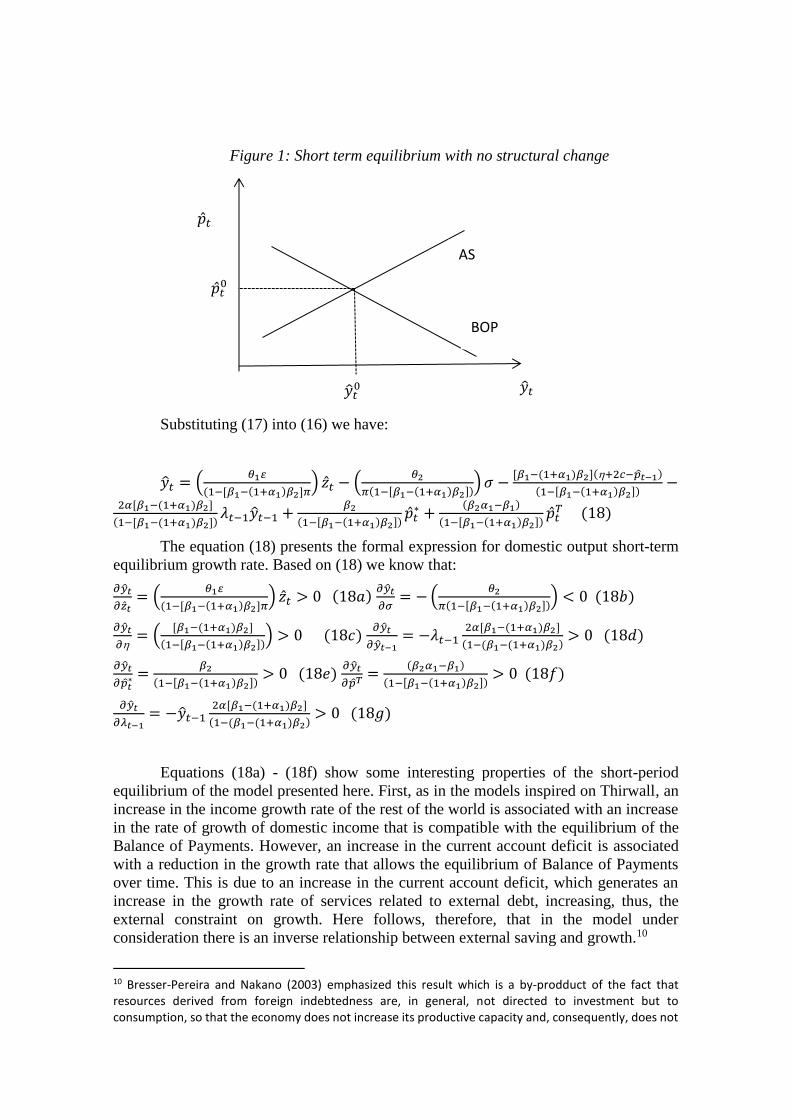
Figure 1: Short term equilibrium with no structural change
Substituting (17) into (16) we have:
�̂�𝑡 = (𝜃1𝜀
(1−[𝛽1−(1+𝛼1)𝛽2]𝜋) �̂�𝑡 − (
𝜃2
𝜋(1−[𝛽1−(1+𝛼1)𝛽2])) 𝜎 −
[𝛽1−(1+𝛼1)𝛽2](+2𝑐−𝑝𝑡−1)
(1−[𝛽1−(1+𝛼1)𝛽2])−
2𝛼[𝛽1−(1+𝛼1)𝛽2]
(1−[𝛽1−(1+𝛼1)𝛽2])𝜆𝑡−1�̂�𝑡−1 +
𝛽2
(1−[𝛽1−(1+𝛼1)𝛽2])�̂�𝑡
∗ +(𝛽2𝛼1−𝛽1)
(1−[𝛽1−(1+𝛼1)𝛽2])�̂�𝑡
𝑇 (18)
The equation (18) presents the formal expression for domestic output short-term
equilibrium growth rate. Based on (18) we know that:
𝜕�̂�𝑡
𝜕�̂�𝑡= (
𝜃1𝜀
(1−[𝛽1−(1+𝛼1)𝛽2]𝜋) �̂�𝑡 > 0 (18𝑎)
𝜕�̂�𝑡
𝜕𝜎= − (
𝜃2
𝜋(1−[𝛽1−(1+𝛼1)𝛽2])) < 0 (18𝑏)
𝜕�̂�𝑡
𝜕= (
[𝛽1−(1+𝛼1)𝛽2]
(1−[𝛽1−(1+𝛼1)𝛽2])) > 0 (18𝑐)
𝜕�̂�𝑡
𝜕�̂�𝑡−1= −𝜆𝑡−1
2𝛼[𝛽1−(1+𝛼1)𝛽2]
(1−(𝛽1−(1+𝛼1)𝛽2)> 0 (18𝑑)
𝜕�̂�𝑡
𝜕𝑝𝑡∗ =
𝛽2
(1−[𝛽1−(1+𝛼1)𝛽2])> 0 (18𝑒)
𝜕�̂�𝑡
𝜕𝑝𝑇=
(𝛽2𝛼1−𝛽1)
(1−[𝛽1−(1+𝛼1)𝛽2])> 0 (18𝑓)
𝜕�̂�𝑡
𝜕𝜆𝑡−1= −�̂�𝑡−1
2𝛼[𝛽1−(1+𝛼1)𝛽2]
(1−(𝛽1−(1+𝛼1)𝛽2)> 0 (18𝑔)
Equations (18a) - (18f) show some interesting properties of the short-period
equilibrium of the model presented here. First, as in the models inspired on Thirwall, an
increase in the income growth rate of the rest of the world is associated with an increase
in the rate of growth of domestic income that is compatible with the equilibrium of the
Balance of Payments. However, an increase in the current account deficit is associated
with a reduction in the growth rate that allows the equilibrium of Balance of Payments
over time. This is due to an increase in the current account deficit, which generates an
increase in the growth rate of services related to external debt, increasing, thus, the
external constraint on growth. Here follows, therefore, that in the model under
consideration there is an inverse relationship between external saving and growth.10
10 Bresser-Pereira and Nakano (2003) emphasized this result which is a by-prodduct of the fact that resources derived from foreign indebtedness are, in general, not directed to investment but to consumption, so that the economy does not increase its productive capacity and, consequently, does not
AS
BOP
�̂�𝑡0
�̂�𝑡0
�̂�𝑡
�̂�𝑡
Another interesting result of the model refers to the impact of increase in rate of
growth of labor force on the outout growth rate compatible with the equilibrium in the
balance of payments. According to equation (18c) the impact is positive. This is due to
an increase in the rate of growth of the labor force which, ceteris paribus, generates a
reduction on wage inflation, thus leading to a reduction on the domestic inflation rate.
Reducing the pace of the domestic price inflation results in a depreciation of the real
exchange rate, this increases the pace of export growth and slows down the growth of
imports, thus increasing the rate of output growth that is compatible with the balance of
payments equilibrium.
In equation (18d) we find that an increase in the growth rate of the output in the
previous period generates an increase of the growth rate of the outout in current period.
This result is a simple consequence of the existence of static and dynamic economies of
scale. In fact, the increase in ouput in the previous period generates an increase in
productivity in the current period, which results in a reduction of the domestic inflation
rate and, ceteris paribus, in a depreciation of real exchange rate. In this context, there will
be an increase in the rate of growth of exports and a reduction in the rate of growth of
imports, thus leading to an increase in the output growth rate which is compatible with
the balance of payments equilibrium.
Equation (18e) shows that an increase in international inflation is associated with
an increase in the output growth rate that is compatible with the balance of payments
equilibrium. The interpretation of this result is trivial.
Equation (18f) shows the most interesting result of the short-run equilibrium of
the model. We note that raising the medium-term inflation target is associated with an
increase in the output growth rate that is compatible with the balance of payments
equilibrium. In this way, monetary policy is not neutral in the short period. This is due to
the following: if the monetary authority raises the medium-term inflation target, given the
domestic inflation rate - or, equivalently, considering a reduction of the interest rate,
ceteris paribus – there will be an increase in the depreciation rate of the nominal exchange
rate leading the real exchange rate to depreciate. Since Marshall-Lerner’s condition is
valid, it follows that there will be an increase in the rate of growth of exports and a
reduction in the rate of growth of imports, making the output growth rate compatible with
the balance of payments equilibrium to increase. Hence, changes in the level of domestic
interest rate have impact on output growth, making monetary policy non-neutral in the
short period.
Finally, equation (18g) shows the impact of changes in the share of manufacturing
industry in the previous period on output growth; In this equation we can see that the
greater the share of manufacturing industry in the economy, the greater will the economic
growth and the lower will the rate of inflation, due to the productivity gains that this sector
generates and spreads over the whole economy.
Substituting (18) in (17), we have:
�̂�𝑡 = (𝜃1𝜀
(1−[𝛽1−(1+𝛼1)𝛽2]𝜋) �̂�𝑡 − (
𝜃2
𝜋(1−[𝛽1−(1+𝛼1)𝛽2])) 𝜎 −
(+2𝑐−𝑝𝑡−1)
(1−[𝛽1−(1+𝛼1)𝛽2])−
2𝛼
(1−(𝛽1−(1+𝛼1)𝛽2)𝜆𝑡−1�̂�𝑡−1 +
𝛽2
(1−[𝛽1−(1+𝛼1)𝛽2])�̂�𝑡
∗ +(𝛽2𝛼1−𝛽1)
(1−[𝛽1−(1+𝛼1)𝛽2])�̂�𝑡
𝑇 (19)
increase the ability to meet external debt commitments. In this way, debt service increases its ratio in proportion of domestic income and limits it to the extent that it diverts resources that could be channeled to other purposes.

Based on (19), we may conclude that:
𝜕𝑝𝑡
𝜕𝑝𝑡−1=
1
(1−[𝛽1−(1+𝛼1)𝛽2])> 0(19𝑎)
𝜕𝑝𝑡
𝜕�̂�𝑡= (
𝜃1𝜀
(1−[𝛽1−(1+𝛼1)𝛽2]𝜋) > 0 (19𝑏)
𝜕𝑝𝑡
𝜕𝜎= − (
𝜃2
𝜋(1−[𝛽1−(1+𝛼1)𝛽2])) < 0 (19𝑐)
𝜕𝑝𝑡
𝜕= −
1
(1−[𝛽1−(1+𝛼1)𝛽2])< 0 (19𝑑)
𝜕𝑝𝑡
𝜕�̂�𝑡−1= −𝜆𝑡−1
2𝛼
(1−(𝛽1−(1+𝛼1)𝛽2)< 0(19𝑒)
𝜕𝑝𝑡
𝜕𝑝𝑡∗ =
𝛽2
(1−[𝛽1−(1+𝛼1)𝛽2])> 0 (19𝑓)
𝜕𝑝𝑡
𝜕𝑝𝑇=
(𝛽2𝛼1−𝛽1)
(1−[𝛽1−(1+𝛼1)𝛽2])> 0 (19𝑔)
𝜕𝑝𝑡
𝜕𝜆𝑡−1= −
2𝛼�̂�𝑡−1
(1−(𝛽1−(1+𝛼1)𝛽2)< 0(19ℎ)
From the expressions (19a) - (19g) we can conclude that equilibrium short-run
domestic inflation rate is a positive function of the inflation rate of the previous period,
of the income growth rate of the rest of the world, of the inflation rate of the rest of the
world and the medium-term inflation target; and an inverse function of the current account
deficit as a proportion of GDP, labor force growth rate, domestic output growth rate, and
manufacturing share of the previous period.
2.2 – Balanced Growth: Existence and Stability
Along to the balanced growth path, we have:
�̂�𝑡 = �̂�𝑡−1 = �̂� (20) �̂�𝑡 = �̂�𝑡−1 = �̂� (21) 𝜆𝑡 = 𝜆𝑡−1 = 𝜆 (22)
Substituting (21) and (22) in (17), we have:
�̂� = + 2𝑐
1 − 2𝜆𝛼 (23)
Equation (23) shows the growth rate of the output along the balanced growth path,
which is called the natural growth rate. For �̂�> 0 it is necessary and sufficient that αλ
<0.5, since the numerator is positive and therefore the denominator will determine the
signal of the equation. Based on this result, we can verify that the Kaldor-Verdoorn
Coefficient is of fundamental importance to ensure the existence of a positive output
growth rate.
Moreover, the existence of a balanced growth path requires a limited value for the
Kaldor-Verdoorn Coefficient, that is, the extent of static and dynamic economies of scale
cannot be very large, since otherwise they would cause instability and would not sustain
a steady-state outcome. It is important to emphasize that this coefficient is the source of
dynamic instability in the economy, since it reinforces possible deviations from the
equilibrium path.
We also verified that the natural growth rate depends only on the parameters of
the labor productivity growth function, the manufacturing share in the economy and the
labor force growth rate, and is therefore independent of monetary policy. It follows that
in this version of the Kaldorian growth model money is neutral in the long run.
Substituting (20) and (21) on (16) we have:
�̂� = (𝜃1𝜀
𝜋) �̂� − (
𝜃2
𝜋) 𝜎 + [𝛽1 − (1 + 𝛼1)𝛽2]�̂� + 𝛽2�̂�∗ + (𝛽2𝛼1 − 𝛽1) �̂�𝑇(24)

Equation (24) presents the locus of the combinations between �̂� and �̂� for which
the balance of payments is in equilibrium along the balanced growth path. Substituting
(23) into (24), we obtain:
�̂� = + 2𝑐
[𝛽1 − (1 + 𝛼1)𝛽2](1 − 2𝜆𝛼)−
𝜃1
[𝛽1 − (1 + 𝛼1)𝛽2]
𝜀
𝜋𝑧
+𝜃2
[𝛽1 − (1 + 𝛼1)𝛽2]𝜋𝜎 −
𝛽2
[𝛽1 − (1 + 𝛼1)𝛽2]�̂�∗ −
(𝛽2𝛼1 − 𝛽1)
[𝛽1 − (1 + 𝛼1)𝛽2]�̂�𝑇 (25)
The visualization of the determination of the long-term equilibrium values of �̂�
and �̂� can be made by means of figure 2 below:
Figure 2: Long-term equilibrium without structural change.
Once the conditions of existence of the balanced growth trajectory have been
defined, we must do the stability analysis.
The system formed by equations (16) and (17) has an intrinsic dynamic, which
can be presented by the following system of finite difference equations:
∆�̂�𝑡 = �̂�𝑡 − �̂�𝑡−1 = (𝜃1𝜀
𝜋) �̂�𝑡 − �̂�𝑡−1 − (
𝜃2
𝜋) 𝜎 + [𝛽1 − (1 + 𝛼1)𝛽2]�̂�𝑡 + 𝛽2�̂�𝑡
∗ +
(𝛽2𝛼1 − 𝛽1) �̂�𝑇 (16𝑎)
∆�̂�𝑡 = �̂�𝑡 − �̂�𝑡−1 = �̂�𝑡 − − 2(𝑐 + 𝛼𝜆𝑡−1�̂�𝑡−1) (17𝑎)
According to Shone (1997), in order to make this system stable, converging to
equilibrium, two conditions are necessary, namely11:
i. [𝛽1 − (1 + 𝛼1)𝛽2](1 − 2𝛼𝜆)<0
ii. [𝛽1 − (1 + 𝛼1)𝛽2](1 + 2𝛼𝜆)<2
As it has already been defined in (16) that 𝛽1 > 0, 𝛽2 > 0 and 𝛽1 < 𝛼1𝛽2,
consequently, it necessarily remains that 0.5> αλ - which has also been defined in (23) -
to satisfy the first constraint. Already to meet the second constraint it is sufficient that
αλ> 0; which is perfectly reasonable assumption. It follows that, once respecting all the
restrictions imposed so far, the system is stable and therefore converges to the equilibrium
positions defined at (23) and (25). Annex I details how this result is achieved.
11 See Annex I
�̂� = + 2𝑐
1 − 2𝜆𝛼 �̂�
�̂�

3 – Growth Model with Structural Change
3.1 –Dynamics of Structural Change
In the previous section, it was considered through equation (9) that the growth rate
of productivity is determined by the output growth rate, given the Kaldor-Verdoorn
coefficient and the share of manufatuing in domestic output.
In this section, we will take consider manufacturing share in output to be an
endogenous variable and then analyze its effects over the system's long-term equilibrium
structure.
The Recent literature related to the Structuralist Delopment Macroeconomics12
insists on the central role of the real exchange rate as an explanatory variable for the
growth or reduction of the share of manufacturing industry in domestic output, especially
in developing economies. According to this literature, an overvalued exchange rate, that
is, an exchange rate that is below to the level that makes the domestic industries operating
with the state of the art techonology to be competitive in the international market, leads
to a progressive reduction of the manufacturing share in output, since this situation
induces a growing overseas transfer of productive activities (see Bresser-Pereira, Oreiro
and Marconi, 2014, 2015). This level of the exchange rate is called the industrial
equilibrium. Thus, a situation of exchange rate overvaluation is associated with a negative
structural change on the economy, which may be called premature de-industrialization
(Palma, 2005). An undervalued exchange rate, that is, above the level of industrial
equilibrium, would have the opposite effect, the one of inducing a transfer of productive
activities into domestic economy, thus increasing the manufacturing share in domestic
output.
The equation that defines the rate of change of manufacturing share in the GDP
can be written as:
�̂�t =∩ [ψ𝑡 − ψi ] (26)
In which �̂�t is the change in industry share in the product, ψi is the "industrial
equilibrium" real exchange rate of the economy indicated by the superscript i, ψ𝑡 Is the
real exchange rate of the previous period, ∩ is a parameter that reflects the sensitivity of
the impact of the real exchange differential in relation to its "industrial equilibrium" on
the variation of the industry share.
On the other hand, we know that the real exchange rate variation over time can be
written as:
ψ̂𝑡 = �̂�𝑡 + �̂�𝑡∗ − �̂�𝑡(27)
By inserting equations (6b) and (25) into (27), we will have:
ψ̂𝑡 = −α1[�̂�𝑡(α, 𝜆,, 𝜀, 𝜋, 𝜎, �̂�𝑡∗, �̂�𝑇) − �̂�𝑇] + [�̂�𝑡
∗ − �̂�𝑡(α, 𝜆,, 𝜀, 𝜋, 𝜎, �̂�𝑡∗, �̂�𝑇)](27a)
Equation (27a) defines the variation of the real exchange rate as a function of the
gap between domestic inflation and the inflation target and the gap between international
inflation and domestic inflation.
12 See Bresser-Pereira, Oreiro e Marconi (2014, 2015)
3.2 Long-Term Equilibrium and Stability Analysis
Equations (26) and (27a) describe the dynamics of the economy with structural
change, that is, in the case where the share of industry in the product varies over time,
depending on the relation between the current value of the exchange rate and the
Industrial equilibrium level.
The long-run equilibrium of the system corresponds to a situation in which both
the real exchange rate and the share of the industry in the product are kept constant over
time.
Under these conditions, we must:
�̂�t = 0 (28a) ; ψ̂𝑡 = 0 (28𝑏)
Substituting (28a) in (26), we have:
ψ = ψ𝑖 (29)
That is, in the long-run equilibrium position of the system, the real exchange rate
is constant and equal to the level corresponding to the industrial equilibrium.
Substituting (28b) into (27a), we have:
α1[�̂�𝑡(α, 𝜆,, 𝜀, 𝜋, 𝜎, �̂�𝑡∗, �̂�𝑇) − �̂�𝑇] = �̂�𝑡
∗ − �̂�𝑡(α, 𝜆,, 𝜀, 𝜋, 𝜎, �̂�𝑡∗, �̂�𝑇)(30)
Reorganizing equation (30), we will find the domestic inflation rate that is
compatible with the maintenance of the real exchange rate at a constant level over time.
�̂�𝑡 =1
(1+α1) �̂�𝑡
∗ +α1
(1+α1)�̂�𝑇(30a)
In equation (25) presented in the previous section we obtained the value of the
domestic inflation rate for which the economy is in its balanced growth path, given the
industry's share of the product. In order to not have an over-determined model, that is,
with more equations than unknowns variables, it is necessary to add some other
endogenous variable to the system. It is clear that the variable that has to be endogenous
is the share of the industry in the product, which will be determined by the making the
equations (25) and (30a) equals. In this way, we have:
𝜆∗ = (1
2𝛼) (
+2𝑐
[𝛽1−(1+𝛼1)𝛽2]) {(
𝜃2
[𝛽1−(1+𝛼1)𝛽2]𝜋) 𝜎 − [(
𝜃1
[𝛽1−(1+𝛼1)𝛽2]) (
𝜀
𝜋) 𝑧∗ +
(1
(1+α1)+
𝛽2
[𝛽1−(1+𝛼1)𝛽2]) �̂�∗ + (
α1
(1+α1)+
(𝛽2𝛼1−𝛽1)
[𝛽1−(1+𝛼1)𝛽2]) �̂�𝑇]}
−1
(31)
Equation (31) presents the long-run equilibrium value for the industry's
participation in the product. The share of industry in the product is adjusted so that the
inflation rate for which the real exchange rate is constant over time is equal to inflation
rate that makes the balance of payments restriction compatible with aggregate supply.
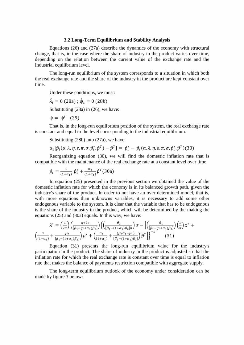
The long-term equilibrium outlook of the economy under consideration can be
made by figure 3 below:

Figure 3 – Long Term Equilibrium with Structural Change.
To analyze the stability of the model, we will linearize the model around its
position of long-term equilibrium, using the first term of Taylor's expansion (Sargent,
1987, pp. 29-30)13. In this way, we have to:
[�̂�t
ψ̂𝑡
] = [
0 ∩
−(1 + 𝛼1)𝜕�̂�𝑡
𝜕𝜆𝑡 0 ] [
𝜆𝑡 − 𝜆∗
ψ𝑡 − ψ𝑖] (32)
The Jacobian matrix [0 ∩
−(1 + 𝛼1)𝜕𝑝𝑡
𝜕𝜆𝑡 0 ] has trace equal to zero and
determinant equal to ∩ (1 + 𝛼1)𝜕𝑝𝑡
𝜕𝜆𝑡< 0. It follows that the dynamics of the system
around the long-term equilibrium position is characterized by a saddle path (Takayama,
1993, p.408). This means that there is only one convergent path, all the others are
divergent. In this context, we will adopt the Sargent and Wallace (1973) methodology of
considering only the convergent trajectory as the only one possible for the economy under
consideration.To do so, we will assume that the level of the real exchange rate adjusts
instantly to put the economy exactly on the convergent path. This hypothesis will have
strong implications for the effects of variations in the inflation target over the real
exchange rate path, as we will see in the next section.
3.3 Non Neutrality of Monetary Policy
In the Kaldorian model with no structural change presented in section 2, we saw
that the monetary policy was neutral in the long run, since changes in the inflation target
or in the inflation aversion coefficient of the monetary policy rule had no impact on the
rate GDP growth along the balanced growth path.
We will now assess whether the result of monetary policy neutrality remains valid
in a model with structural change, that is, if in a context where the share of industry in the
product is an endogenous variable that adjusts to the gap between the current value of the
13 This procedure, in effect, has the effect of transforming the system of equations of finite differences into a system of differential equations.
�̂�t = 0
ψ̂𝑡 = 0
𝜆∗ 𝜆
ψ𝑖
ψ
real rate of Exchange rate and its industrial equilibrium value, it remains true that changes
in the inflation target do not affect the real variables of the economy.
We know from equation (6b) that raising the inflation target is associated with a
depreciation of the exchange rate. This is due to the fact that raising the inflation target
allows the monetary authority to reduce the domestic interest rate, a reduction that
generates an outflow of capital from the country and, consequently, a depreciation of the
nominal exchange rate. The devaluation of the nominal exchange rate, given the domestic
rate of inflation, should result in a devaluation of the real exchange rate, which, in turn,
will induce an increase in the share of the industry in the economy. This increase in the
industry share, in turn, will increase the Kaldor-Verdoorn coefficient in equation (23),
which will result in an increase in the growth rate of the product along the balanced
growth path.
The validity of this reasoning can be attested by the differentiation of (31a) with
respect to 𝜆 and �̂�𝑇. So we have:
𝜕𝜆
𝜕𝑝𝑇= (
1
2𝛼) (
+2𝑐
[𝛽1−(1+𝛼1)𝛽2]) {(
𝜃2
[𝛽1−(1+𝛼1)𝛽2]𝜋) 𝜎 − [(
𝜃1
[𝛽1−(1+𝛼1)𝛽2]) (
𝜀
𝜋) 𝑧∗ +
(1
(1+α1)+
𝛽2
[𝛽1−(1+𝛼1)𝛽2]) �̂�∗ + (
α1
(1+α1)+
(𝛽2𝛼1−𝛽1)
[𝛽1−(1+𝛼1)𝛽2]) �̂�𝑇]}
−2
[α1
(1+α1)+
(𝛽2𝛼1−𝛽1)
[𝛽1−(1+𝛼1)𝛽2]] >
0 (33)
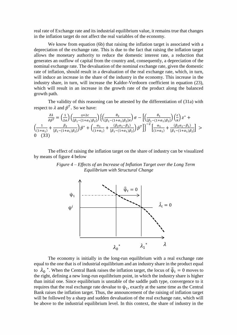
The effect of raising the inflation target on the share of industry can be visualized
by means of figure 4 below
Figure 4 – Effects of an Increase of Inflation Target over the Long Term
Equilibrium with Structural Change
The economy is initially in the long-run equilibrium with a real exchange rate
equal to the one that is of industrial equilibrium and an industry share in the product equal
to 𝜆0 ∗. When the Central Bank raises the inflation target, the locus of ψ̂𝑡 = 0 moves to
the right, defining a new long-run equilibrium point, in which the industry share is higher
than initial one. Since equilibrium is unstable of the saddle path type, convergence to it
requires that the real exchange rate devalue to ψ1, exactly at the same time as the Central
Bank raises the inflation target. Thus, the announcement of the raising of inflation target
will be followed by a sharp and sudden devaluation of the real exchange rate, which will
be above to the industrial equilibrium level. In this context, the share of industry in the
�̂�t = 0
ψ̂𝑡 = 0
𝜆0∗
𝜆
ψ𝑖
ψ1
𝜆1∗

product will gradually increase until it reaches its new long-term equilibrium point, 𝜆1∗.
Throughout the adjustment path towards the new equilibrium point, the real exchange
rate will be appreciated, albeit it remains above to level of equilibrium point. Therefore,
raising the inflation target results in (i) a permanent increase in the share of industry in
the GDP – and consequently an increase in long-term growth rate – and a (ii) temporary
devaluation of the real exchange rate.
4 – Conclusions
Throughout this paper we presented a kaldorian model that incorporates a balance
of payments constraint similar to the one developed by Moreno-Brid (2003), as well as
incorporating into the dynamic equation of productivity growth the idea that the Kaldor-
Verdoorn coefficient depends on the industry share of the product. These innovations
represent a step forward not only to eliminate the inconsistency present in growth models
with balance of payments constraint, which are unable to reconcile the balance of
payments constraint with the supply side of the economy; as well as in the sense of
permitting the occurrence of endogenous structural change associated with the
misalignment of the real exchange rate, defined as the difference between the current level
of the real exchange rate and the value corresponding to the "industrial equilibrium".
Thus, the model presented here allows integration between Kaldorian growth models led
by aggregate demand and the Structuralist Macroeconomics of Development.
5 – References
BOTTA, A. (2009). “A structuralist north-south model on structural change, economic
growth and catching-up”. Structural change and Economic Dynamics, v. 20, pp. 61-73.
BRESSER-PEREIRA, L.C; NAKANO, Y. (2003). “Crescimento Econômico com
Poupança Externa?”. Revista de Economia Política, v.22, n.2.
BRESSER-PEREIRA, L.C; OREIRO, J.L; MARCONI, N. (2014). “A Theoretical
Framework for New Developmentalism” In: BRESSER-PEREIRA, L.C; KREGEL, J;
BURLAMAQUI, L. (orgs.). Financial Stability and Growth: perspectives on financial
regulation and new developmentalism. Routledge: Londres.
-------------------- (2015). Developmental Macroeconomics: new delopmentalism as a
growth strategy. Routledge: Londres.
CARLIN, W; SOSKICE, D. (2006). Macroeconomics: imperfections, institutions and
policies. Oxford University Press: Oxford.
FRENKEL (2004). “Real Exchange Rate and Employment in Argentina, Brazil, Chile
and Mexico”. Centro de Estudios de Estado y Sociedad.
GABRIEL, L.F; OREIRO, J.L; GONZAGA, F. (2015). “Um Modelo Norte-Sul de
Crescimento Econômico, Hiato Tecnológico, Mudança Estrutural e Taxa de Câmbio
Real”. Texto para Discussão 010/2015, Instituto de Economia da Universidade Federal
do Rio de Janeiro.
McCOMBIE, J.S.L; ROBERTS, M. (2002). “The Role of the Balance of Payments in
Economic Growth” In: SETTERFIELD, M. (org.). The Economics of Demand-Led
Growth. Edward Elgar: Aldershot.

MORENO-BRID, J.C. (2003). “Capital Flows, Interest payments and the Balance of
Payments constrained growth model: A Theoretical and Empirical Analysis”.
Metroeconomica, pp. 346-65.
OREIRO, J.L; PUNZO; L; ARAUJO, E. (2012). “Macroeconomic constraints to growth
of Brazilian economy: diagnosis and some policy proposals”. Cambridge Journal of
Economics, 36, pp. 919-939.
OREIRO, J.L. (2009). “A Modified Kaldorian Model of Cumulative Causation”.
Investigación Económica, Vol LXVIII, 268, pp.15-38.
-------------------- (2004). “Autonomia da Política Econômica, fragilidade externa e
equilíbrio do balanço de pagamentos: a teoria econômica dos controles de capitais”.
Economia e Sociedade, Vol. 13, n2.
PALLEY, T. (2002). “Pitfalls in the Theory of Growth: an application to the balance of
payments constrained growth model” In: SETTERFIELD, M. (org.). The Economics of
Demand-Led Growth. Edward Elgar: Aldershot.
PALMA, G (2005).” Four sources of ‘de-industrialisation’ and a new concept of the
Dutch disease”. In: OCAMPO, J. A. (Org.). Beyond reforms: structural dynamics and
macroeconomic vulnerability. Stanford University Press and World Bank.
RAZIN, O.; COLLINS, S. (1997). Real Exchange Rate Misalignments and Growth.
NBER, Working Paper 6147.
RODRIK, D. (2008). “Real Exchange Rate and Economic Growth: Theory and
Evidence”, John F. Kennedy School of Government, Harvard University, Draft, July.
SARGENT, T. (1987). Macroeconomic Theory. Academic Press: Nova Iorque.
SHONE, R. (1997). Economic Dynamics. Cambridge University Press: Cambridge.
TAKAYAMA, A. (1993). Analytical Methods in Economics. The University of Michigan
Press: Nova Iorque.
THIRWALL, A. P. (1979). “The Balance of Payments Constraint as a explanation of
international growth rate differences”. Banca Nazionale Del Lavoro Quarterly Review,
128, pp. 45-53.
THIRLWALL, A.P; HUSSAIN, M.N. (1982). “The Balance of Payments Constraint,
Capital Flows and Growth Rate Differences Between Developing Countries”, Oxford
Economic Papers, November.
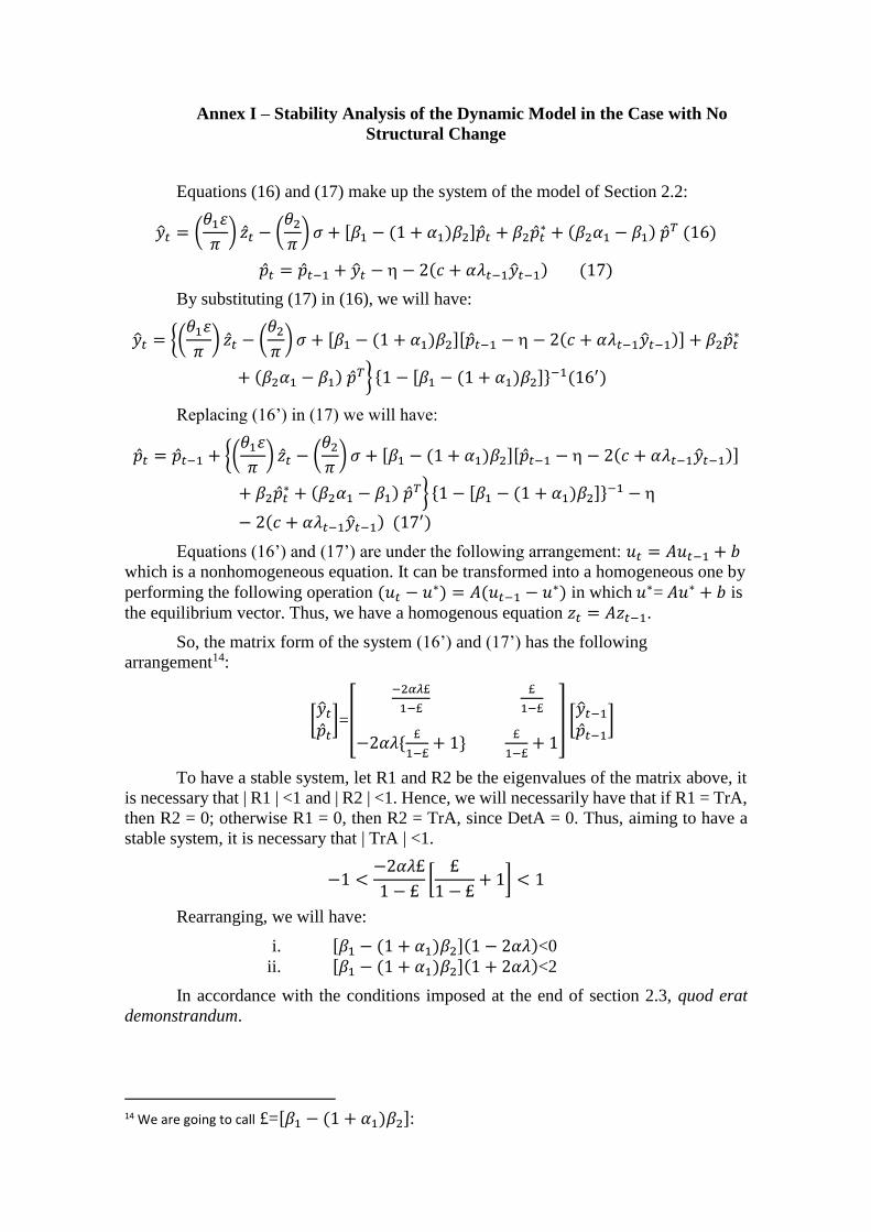
Annex I – Stability Analysis of the Dynamic Model in the Case with No
Structural Change
Equations (16) and (17) make up the system of the model of Section 2.2:
�̂�𝑡 = (𝜃1𝜀
𝜋) �̂�𝑡 − (
𝜃2
𝜋) 𝜎 + [𝛽1 − (1 + 𝛼1)𝛽2]�̂�𝑡 + 𝛽2�̂�𝑡
∗ + (𝛽2𝛼1 − 𝛽1) �̂�𝑇 (16)
�̂�𝑡 = �̂�𝑡−1 + �̂�𝑡 − − 2(𝑐 + 𝛼𝜆𝑡−1�̂�𝑡−1) (17)
By substituting (17) in (16), we will have:
�̂�𝑡 = {(𝜃1𝜀
𝜋) �̂�𝑡 − (
𝜃2
𝜋) 𝜎 + [𝛽1 − (1 + 𝛼1)𝛽2][�̂�𝑡−1 − − 2(𝑐 + 𝛼𝜆𝑡−1�̂�𝑡−1)] + 𝛽2�̂�𝑡
∗
+ (𝛽2𝛼1 − 𝛽1) �̂�𝑇} {1 − [𝛽1 − (1 + 𝛼1)𝛽2]}−1(16′)
Replacing (16’) in (17) we will have:
�̂�𝑡 = �̂�𝑡−1 + {(𝜃1𝜀
𝜋) �̂�𝑡 − (
𝜃2
𝜋) 𝜎 + [𝛽1 − (1 + 𝛼1)𝛽2][�̂�𝑡−1 − − 2(𝑐 + 𝛼𝜆𝑡−1�̂�𝑡−1)]
+ 𝛽2�̂�𝑡∗ + (𝛽2𝛼1 − 𝛽1) �̂�𝑇} {1 − [𝛽1 − (1 + 𝛼1)𝛽2]}−1 −
− 2(𝑐 + 𝛼𝜆𝑡−1�̂�𝑡−1) (17′)
Equations (16’) and (17’) are under the following arrangement: 𝑢𝑡 = 𝐴𝑢𝑡−1 + 𝑏
which is a nonhomogeneous equation. It can be transformed into a homogeneous one by
performing the following operation (𝑢𝑡 − 𝑢∗) = 𝐴(𝑢𝑡−1 − 𝑢∗) in which 𝑢∗= 𝐴𝑢∗ + 𝑏 is
the equilibrium vector. Thus, we have a homogenous equation 𝑧𝑡 = 𝐴𝑧𝑡−1.
So, the matrix form of the system (16’) and (17’) has the following
arrangement14:
[�̂�𝑡
�̂�𝑡]=[
−2𝛼𝜆£
1−£
£
1−£
−2𝛼𝜆{£
1−£+ 1}
£
1−£+ 1
] [�̂�𝑡−1
�̂�𝑡−1]
To have a stable system, let R1 and R2 be the eigenvalues of the matrix above, it
is necessary that | R1 | <1 and | R2 | <1. Hence, we will necessarily have that if R1 = TrA,
then R2 = 0; otherwise R1 = 0, then R2 = TrA, since DetA = 0. Thus, aiming to have a
stable system, it is necessary that | TrA | <1.
−1 <−2𝛼𝜆£
1 − £[
£
1 − £+ 1] < 1
Rearranging, we will have:
i. [𝛽1 − (1 + 𝛼1)𝛽2](1 − 2𝛼𝜆)<0
ii. [𝛽1 − (1 + 𝛼1)𝛽2](1 + 2𝛼𝜆)<2
In accordance with the conditions imposed at the end of section 2.3, quod erat
demonstrandum.
14 We are going to call £=[𝛽1 − (1 + 𝛼1)𝛽2]: