REAL ESTATE PRICES AND CORPORATE INVESTMENT …

Banque de France Working Paper #626 April 2017

REAL ESTATE PRICES AND CORPORATE INVESTMENT: THEORY AND EVIDENCE OF HETEROGENEOUS EFFECTS ACROSS FIRMS Denis Fougère1, Rémy Lecat2, Simon Ray3

April 2017, WP #626

ABSTRACT In this paper, we investigate the effect of real estate prices on productive investment. We build a simple theoretical framework of firms’ investment with credit rationing and real estate collateral. We show that real estate prices affect firms’ borrowing capacities through two channels. An increase in real estate prices raises the value of the firms’ pledgeable assets and mitigates the agency problem characterizing the creditor-entrepreneur relationship. It simultaneously cuts the expected profit due to the increase in the cost of inputs. While the literature only focuses on the first channel, the identification of the second channel allows for heterogeneous effects of real estate prices on investment across firms. We test our theoretical predictions using a large French database. We do find heterogeneous effects of real estate prices on productive investment depending on the position of the firms in the sectoral distributions of real estate holdings. Our preferred estimates indicate that a 10% increase in real estate prices causes a 1% decrease in the investment rate of firms in the first decile of the distribution but a 6% increase in the investment rate of firms belonging to the last decile.4

Keywords: Firms’ investment, Real estate prices, Collateral channel, Financial constraints. JEL classification: D22, G30, O52, R30

1 CNRS, OSC and LIEPP (Sciences Po, Paris), Banque de France, CEPR and IZA, [email protected] 2 Banque de France, [email protected] 3 Banque de France and Aix-Marseille University (Aix-Marseille School of Economics), CNRS, EHESS, [email protected] 4 The authors would like to thank, without implicating, Philippe Aghion, Gilbert Cette, Thomas Chaney, Laurent Gobillon, Johan Hombert, Pauline Gandré, Claire Lelarge, Conor O'Toole and Jean-Marc Robin for helpful comments and suggestions. We also thank seminar participants at Aix-Marseille School of Economics, the Central Bank of Ireland workshop on "Banking, Credit and Macroprudential Policy", the Banque de France research seminar, the Royal Economic Society 2016 conference and the 2016 Annual meeting of the French Economic Association. Denis Fougère acknowledges support from the French National Research Agency’s (ANR) “Investissements d’Avenir” grants ANR-11-LABX-0091 (LIEPP). Working Papers reflect the opinions of the authors and do not necessarily express the views of the Banque de France. This document is available on publications.banque-france.fr/en

https://publications.banque-france.fr/en

Banque de France Working Paper #626 ii

NON-TECHNICAL SUMMARY In this paper, we estimate the effect of real estate prices on productive investment (i.e., machines, equipment and intangible assets), focusing on potential heterogeneous impacts depending on the composition of the firms' assets. We first formalize the link between real estate prices and productive investment in a context where credit markets are frictional thanks to a partial equilibrium model, we then bring our theoretical predictions to the data to show that an increase in local real estate prices hinders the investment of firms that do not benefit from a collateral channel. From the late nineties to the financial crisis, real estate prices in many advanced countries have experienced a boom, unprecedented in size and duration. This has led to question the impact of this boom on productive investment. In countries where a bust has followed the boom like Spain, the adjustment revealed a significant capital misallocation and led to a rebalancing towards the exporting sector (Cette, Fernald and Mojon, 2016). On the contrary, in France, real estate prices did not correct significantly and remained higher than in the nineties relative to consumer or equipment prices. Yet, France is also subject to questioning about the impact of the real estate prices boom on sectoral allocation and on productive investment (Askenazy, 2016): did the real estate boom alter the allocation of investment towards less productive sectors or firms? The literature has focused so far on the collateral channel that connects real estate prices to productive investment. In an imperfect credit market, collateral pledging enhances the firms' borrowing capacities. The ability of the lenders to seize pledged collateral increases the debt capacity of the borrowers as it mitigates the agency problem in this external financing relationship. The extent to which the borrowing constraint is relaxed by collateral pledging depends on the collateral liquidation value. In these empirical studies, real estate prices are regarded as mere shifters of the pledgeable assets' value which determines the borrowing capacities of firms. Yet, an increase in real estate prices surely raises the value of the pledgeable assets and mitigates the agency

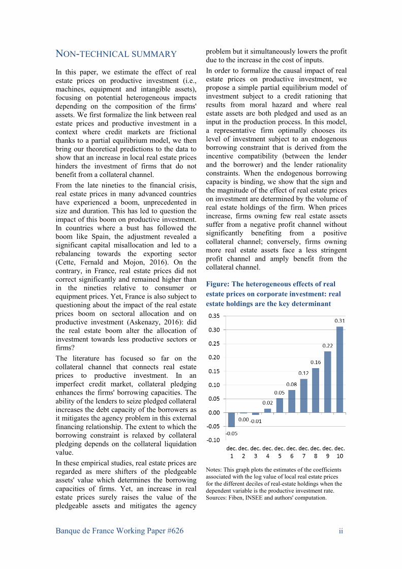
problem but it simultaneously lowers the profit due to the increase in the cost of inputs. In order to formalize the causal impact of real estate prices on productive investment, we propose a simple partial equilibrium model of investment subject to a credit rationing that results from moral hazard and where real estate assets are both pledged and used as an input in the production process. In this model, a representative firm optimally chooses its level of investment subject to an endogenous borrowing constraint that is derived from the incentive compatibility (between the lender and the borrower) and the lender rationality constraints. When the endogenous borrowing capacity is binding, we show that the sign and the magnitude of the effect of real estate prices on investment are determined by the volume of real estate holdings of the firm. When prices increase, firms owning few real estate assets suffer from a negative profit channel without significantly benefiting from a positive collateral channel; conversely, firms owning more real estate assets face a less stringent profit channel and amply benefit from the collateral channel.

Figure: The heterogeneous effects of real estate prices on corporate investment: real estate holdings are the key determinant

Notes: This graph plots the estimates of the coefficients associated with the log value of local real estate prices for the different deciles of real-estate holdings when the dependent variable is the productive investment rate. Sources: Fiben, INSEE and authors' computation.

Banque de France Working Paper #626 iii

We use a large French firm database to confront these predictions with the data. France is a particularly relevant case to test these theoretical predictions as it experienced both a very steep, and yet uncorrected increase in real estate prices. We contribute to the existing literature by showing that the sign and the magnitude of the effect of real estate prices on productive investment are driven by real estate holdings. We notably show that real estate prices have heterogeneous effects on productive investment depending on the position of the firms in the 2-digit sectoral distributions of a normalized measure of real estate holdings

(see the graph presented above). We find a negative impact of an increase in real estate prices on productive investment at the bottom of the distribution, while the effect is highly positive at the upper end of the distribution. Our preferred estimates indicate that a 10% increase in real estate prices causes a 1% decrease in the investment rate of firms in the first decile of the distribution but a 6% increase in the investment rate of firms belonging to the last decile. Our empirical results also suggest that the impact of an increase in real estate prices on aggregate productive capital is positive. The documented heterogeneous effects across firms could link real estate prices dynamics to suboptimal allocation of inputs.

PRIX DE L’IMMOBILIER ET INVESTISSEMENT DES ENTREPRISES : THÉORIE ET ÉLÉMENTS DE PREUVE EMPIRIQUE DES EFFETS HÉTÉROGÈNES RÉSUMÉ Dans cet article, nous étudions les effets des prix de l’immobilier sur l’investissement productif des entreprises. Nous proposons un cadre théorique simple qui permet de rendre compte de l’investissement des entreprises en présence de contraintes de crédit fondées sur le collatéral immobilier. Nous montrons que les prix de l’immobilier influent sur la capacité d’investissement des entreprises via deux canaux. Une hausse des prix accroit la valeur de marché de l’actif collatéralisable et atténue les effets du problème de type principal-agent qui caractérise la relation entre le créditeur et l’entrepreneur. Simultanément, cette hausse diminue le profit attendu du fait de l’accroissement du coût d’un facteur de production. Alors que la littérature s’est principalement intéressée à ce premier canal, l’identification du second met en lumière l’effet potentiellement hétérogène de la dynamique des prix de l’immobilier sur l’investissement des entreprises. En mobilisant une base de données d’entreprises françaises, nous trouvons des effets hétérogènes des prix de l’immobilier sur l’investissement des entreprises selon leur position dans la distribution sectorielle du niveau de détention d’actifs immobiliers. Une hausse de 10 % des prix de l’immobilier induit une baisse de 1 % du taux d’investissement des entreprises situées dans le premier décile alors que cette même hausse accroît de 6 % le taux d’investissement des entreprises situées dans le dernier décile.

Mots-clés : Investissement des entreprises, prix de l’immobilier, canal du collatéral, contrainte financière. Les Documents de travail reflètent les idées personnelles de leurs auteurs et n'expriment pas nécessairement la position de la Banque de France. Ce document est disponible sur publications.banque-france.fr

https://publications.banque-france.fr/

https://publications.banque-france.fr/

1 Introduction

This paper estimates the effect of real estate prices on productive investment (i.e., machines,equipment and intangible assets), focusing on potential heterogeneous impacts dependingon the composition of the firms’ assets.

From the late nineties to the financial crisis, real estate prices in many advanced coun-tries have experienced a boom, unprecedented in size and duration. These booms led tosignificant capital misallocation across sectors and firms (Cette, Fernald, and Mojon, 2016).In France, despite a decrease during the crisis, the price level remains much higher than inthe nineties relative to consumer or equipment prices and the question is raised as to theimpact of the real estate prices boom on sectoral allocation and on productive investment(Askenazy, 2013).

While the literature has focused on the collateral channel of real estate prices, withmonotonous effects on investment, we take into account both this collateral channel anda factor cost channel, which yield heterogeneous effects of real estate prices on produc-tive investment of credit-constrained firms. These results are theoretically formalized andsubstantiated by empirical analyses performed on a large French firm-level database. Weshow that both the sign and the magnitude of their effect depend on the firms’ real estateholdings.

In an imperfect credit market, collateral pledging enhances the firms’ borrowing capaci-ties. The ability of the lenders to seize pledged collateral increases the debt capacity of theborrowers as it mitigates the agency problem in this external financing relationship (Bergerand Udell, 1990). The extent to which the borrowing constraint is relaxed by collateralpledging depends on the collateral liquidation value. Real estate assets often constitutethe bulk of the firms’s pledgeable assets since they are easily redeployable and have a longlifespan. Collecting data on the financing behavior of 91 banks in 45 countries, Beck,Demirguc-Kunt, and Martinez Peria (2008) find that more than three-quarters of banks re-quire collateral to make business loans and that real estate is the most frequently acceptedtype of collateral for business lending, regardless of firms’ size. Through this mechanism,an increase in real estate prices is expected to relax the firms’ borrowing constraint and toease their funding.

The role of this collateral channel has been extensively discussed in the literature onmacroeconomic fluctuations. For instance, Kiyotaki and Moore (1997) show how the inter-action between credit limits and asset prices is a powerful transmission mechanism whichexplains large and persistent comovements in output and asset prices through investmentdynamics. Recent macroeconomic contributions have shed light on the link between landprices and business investment. Liu, Wang, and Zha (2013) develop a macroeconomic modelwhere land is used as a collateral by credit constrained firms. When they estimate theirmodel on aggregate US data, they find that the joint dynamics of land prices and invest-ment is an important mechanism that amplifies and propagates macroeconomic fluctuations.Kaas, Pintus, and Ray (2014) also provide empirical evidence of such a mechanism usingaggregate data from France.

The positive causal relationship between real estate prices and corporate investment,channeled by the collateral value, has also been empirically examined using firm-level data.Based on a large sample of publicly-listed firms in Japan, Gan (2007) finds a significantimpact of collateral value on corporate investment during the five-year period after theland price collapse which occurred in the early 1990s. Chaney, Sraer, and Thesmar (2012)

1

(hereafter CST ) study the sensitivity of investment to real estate collateral value by usingdata from a sample of US publicly-listed firms observed between 1993 and 2007. Theyfind a substantial causal relationship between collateral value and business investment atthe firm level. In a recent contribution focusing on labor market variables, Chaney, Sraer,and Thesmar (2013) document a significant real estate collateral channel by considering alarge database of French firms observed over the period 1998-2007. Interestingly enough,Wu, Gyourko, and Deng (2015) find no evidence of such a mechanism for Chinese firms,suggesting that the transmission mechanism from real estate prices to corporate invest-ment essentially works through credit market frictions. Indeed, the authors argue that thecollateral channel may be altered in the Chinese case by the role played by state-ownedenterprises and government-controlled banks.

In these empirical studies, real estate prices are regarded as mere shifters of the pledge-able assets’ value which determines the borrowing capacities of firms. This view relies onthe credit rationing mechanism, put forward by Hart and Moore (1990) and built aroundthe idea that, because loan agreement can be renegotiated and the entrepreneur is requiredfor the completion of the project, the borrowing capacity only depends on the anticipatedliquidation value of the asset that the lender can seize. In this framework, asset prices havean unambiguous positive effect on the borrowing capacities of firms.

Yet, when as a result of the agency problem characterizing the creditor-entrepreneurrelationship, the borrowing capacity is determined by the expected value of pledged assetsalong with the expected firms’ profit (Tirole, 2010), real estate prices have an equivocalimpact on borrowing capacities. Indeed, real estate prices draw the two components of thisborrowing capacity in opposite directions: an increase in real estate prices raises the valueof the pledgeable assets and mitigates the agency problem but it simultaneously lowers theirprofit due to the increase in the cost of inputs.

In order to formalize the link between real estate prices and productive investment,we propose a simple partial equilibrium model of investment subject to a credit rationingthat results from moral hazard and where real estate assets are both pledged and used asan input in the production process. When investment is determined by the endogenousborrowing capacity, we show that the sign and magnitude of the effect of real estate priceson investment are determined by the volume of real estate holdings of the firm. When pricesincrease, firms owning few real estate assets suffer from a negative profit channel withoutsignificantly benefiting from a positive collateral channel; conversely, firms owning morereal estate assets face a less stringent profit channel and amply benefit from the collateralchannel.

We use a large French firm database to confront these predictions with the data. Franceis a particularly relevant case to test these theoretical predictions as it experienced both avery steep, and yet uncorrected increase in real estate prices, while it registered growingsigns of misallocations, in particular through increasing productivity dispersion across firms(Cette, Corde, and Lecat, 2017). When estimating the effect of real estate prices on produc-tive investment, we face an identification issue resulting from the fact that real estate pricescomove with the business cycle. More specifically, we know that the level of bank credits af-fect both investment and real estate prices (Mora, 2008 and Favara and Imbs, 2015). Thus,real estate prices are correlated with investment opportunities. Following Case, Quigley,and Shiller (2005) and CST , our identification strategy is twofold. First, we analyze the

2

effect of real estate prices at the departement level1 on investment, which is not necessar-ily limited to the departement boundaries. Large firms operating at the national level areexpected to face similar economic conditions but their borrowing capacities follow differentpaths depending on the dynamics of local real estate prices, namely in the departementwhere the firms’ real estate assets are located. Second, within a departement where firmsface the same local economic conditions and thus similar investment opportunities, we cancompare the impact of real estate prices on productive investment across firms with varyinglevel of real estate holdings.

We contribute to the existing literature by showing that, in accordance with the resultsderived from a theoretical model with an endogenous borrowing constraint taking intoaccount firms’ profit, the sign and magnitude of the effect of real estate prices on productiveinvestment are determined by real estate holdings. In particular, we show that real estateprices have heterogeneous effects on productive investment depending on the position of thefirms in the 2-digit sectoral distributions of a normalized measure of real estate holdings.We find a negative impact of an increase in real estate prices on productive investment atthe bottom of the distribution, while the effect is highly positive at the upper end of thedistribution. Our preferred estimates indicate that a 10% increase in real estate prices causesa 1% decrease in the investment rate of firms in the first decile of the distribution but a 6%increase in the investment rate of firms belonging to the last decile. Our empirical resultsalso suggest that the impact of an increase in real estate prices on aggregate productivecapital is positive. Nevertheless, the documented heterogeneous effects across the real estateholdings distribution could link real estate prices dynamics to misallocation of capital.

Our paper is organized as follows. Section 2 presents a tool model from which we deriveour main testable predictions. Section 3 presents data sources and variables. Section 4reports and comments our empirical findings. Section 5 concludes.

2 A simple theoretical framework

We develop a simple model of firms’ productive investment with credit rationing and realestate collateral in the spirit of the one proposed by Chaney, Sraer, and Thesmar (2009).Nevertheless, we introduce two substantial changes that alter the effect of real estate priceson the productive investment of credit-constrained firms. First, we consider an alternativemicro-founded borrowing constraint based on the moral hazard mechanism puts forward byTirole (2010). Second, we treat real estate assets as inputs in the firms’ production process.

2.1 Model setup

In this model, we consider a risk-neutral representative Firm (the “Entrepreneur” or “Bor-rower”) in a small open economy ; the risk free interest rate is r > 0. The Firm is assumedto have a finite horizon and the model has only two dates that correspond to the beginningand the end of a period.

At the beginning of the period, the representative Firm is endowed with capital k0,cash-flow c0 (in units of capital), outstanding debt B0 (in units of capital) owing to anexternal investor, and R0 real estate units. The net debt is defined as the outstanding debt

1A departement is an administrative zone. There are 95 departements in France. Each of them hasapproximately the same geographical size (6, 000 square kilometers), but different population sizes.

3

minus the cash-flow, hence NB0 = B0 − c0.2 The Firm can invest at the beginning of theperiod in a project that yields gross revenue y(k,R, θ) at the end of the period; k is theFirm’s capital made of the initial capital and the investment, hence k = k0 + i where i isthe investment at the beginning of the period; R is the amount of real estate units used bythe Firm and θ is the Firm’s productivity, with θ ∈ [θ, θ].3 The revenue function is twicedifferentiable, increasing with k, R and θ, and concave with k, R and θ. Capital and realestate are also assumed to be partially substitutable and therefore ykR > 0.

The Firm must choose at the beginning of the period the amount of real estate unitsused in its production process. To modulate the real estate facilities, the Firm has accessto a perfectly competitive real estate market and contracts with an outside risk-neutralcounterpart either to rent or to lend real estate units. We denote rl the renting cost of oneunit of real estate over the period; a simple no-arbitrage condition gives rl = rp, where p isthe market price of one real estate unit (in units of capital), with p ∈ [p, p].4 The functioncre denotes the Firm’s real estate cost paid at the end of the period. Note that these realestate costs can also be thought as the user cost of real estate capital of a Firm that borrowsat the risk free interest rate. From what precedes, we have cre(R) = rp(R−R0).

At the end of the period, the Firm is liquidated. The liquidation value corresponds tothe market value of the real estate assets as we assume that k has no outside value.

2.2 Credit rationing

The Firm may need external financing if the initial cash-flow is insufficient to finance in-vestment. The Firm can contract with a deep-pocket, risk-neutral external Investor (or“the Lender”); the Lender behaves competitively in the sense that the loan, if any, makesno profit. A financing contract specifies two transfers (b0; b1) ∈ R2 from the Firm to theInvestor; b0 occurs at the beginning of the period and b1 at the end of the period. Theysatisfy the condition b0 + b1

1+r ≥ B0.5

An essential feature of our model is that the Firm faces credit rationing. Some profitableinvestments may not receive funding. This credit rationing is driven by the asymmetry ofinformation between borrowers and lenders. The mechanism of credit rationing that weintroduce is similar to the one set forth by Tirole (2010). The Lender faces an agencyproblem as the Firm (or “the Borrower”) may mismanage the project. The Borrower caneither “behave” or “misbehave”. Behaving yields the above-described revenue y and noprivate benefit to the Firm. Misbehaving generates a private benefit S > 0 (measured inunits of capital) to the Entrepreneur that can be interpreted as disutility of effort savedby the Entrepreneur when shirking. This private benefit damages the profitability of theproject and induces a fixed loss compared to the optimal revenue; the project yields y − Lwhen the Entrepreneur misbehaves. It is inefficient in the sense that the private benefit to

2We assume k0 ∈ [0, k0]; c0 ∈ [0, c0];B0 ∈ [0, B0] and R0 ∈ [0, R0]. Restrictions on the value of B0 arediscussed below.

3We introduce the Firm’s productivity in this model because the literature on agglomeration economieshas documented the link between local spatial density and productivity (see Combes and Gobillon, 2014 fora recent survey). Introducing productivity in this model renders explicit that changes in productivity canpartially offset the effects of prices on factors’ demand when productivity and prices comove.

4An implicit hypothesis behind this renting rate is that there is no expected capital gain or loss.5In order to discard any case of inevitable default, we assume that the net present value of the Firm is posi-

tive even if there is no initial investment. it implies an upper bound for B0, i.e, B0 ≤ c0+ y(k0,R,θ)−cre(R)+pR01+r

or equivalently, NB0 ≤ y(k0,R,θ)−cre(R)+pR01+r

.

4

the Firm is smaller than the foregone revenue (i.e., S < L) but, as this private benefit isnot shared with the Investor conversely to the revenue, the Firm may prefer to misbehave.We assume that their values are known by both agents. Consequently, to ensure that theFirm will not shirk, the loan agreement between the Firm and the Investor (to be definedbelow) must secure a sufficient stake in the outcome of the project to the Firm. Thus, theproject’s income cannot be fully pledged to the outside Investor and a project may notreceive financing even if the expected profit, when the Firm behaves, exceeds the requiredinvestment plus the interest expenses.

In order to enhance its borrowing capacity, the Firm pledges collateral. We focus ouranalysis on real estate collateral as we have set the outside value of used capital to 0. Thevalue of collateralizable assets corresponds to the market value of the real estate assets, thatis pR0. The financing contract between the Firm and the Investor stipulates how the profitis shared as well as a contingent right for the investor to seize the real estate collateral. Ashare ϕ of the profit goes to the Firm and a share 1−ϕ goes to the investor in order to payback the loan and its interests. If the Firm defaults on the loan, that is to say if the Firmis not in a position to transfer a amount b1 satisfying the above-mentioned condition, theinvestor seizes the collateral and the Firm losses the collateral pledged.6

We assume that L is large enough in comparison to S so that there is no profitableinvestment in case of a misbehavior:

(y − cre − L+ S)− (1 + r)i < 0 (1)

Making this assumption, we insure that the project is funded if and only if the incentivescheme is designed so that the Entrepreneur behaves. Indeed, equation (1) implies:

[(1− ϕ)(y − cre − L)− (1 + r)(i− c0 +B0)] + [ϕ(y − cre − L) + S − (1 + r)c0] < 0 (2)

In the inequality (2), when the second term within square brackets - the profit to theFirm in case of a misbehavior minus the future value of initial cash - is positive, the firstterm within the square brackets - the profit to the Lender in case of a misbehavior minusthe future value of outstanding debt - is negative. Shirking entails defaulting and thus noloan that gives an incentive to the Firm to misbehave will be granted.

From the loan agreement’s structure, we derive an incentive compatibility constraintstating that the share of the profit going to the Firm must insure that the entrepreneur isbetter off behaving:

ϕy ≥ ϕ(y − L) + S − pR0 (3)

This incentive constraint defines a lower limit for ϕ; we denote this limit ϕ = S−pR0

L .The private benefit being smaller than the foregone revenue we have ϕ < 1. The sign of ϕ,that is to say the sign of S−pR0, is crucial as it determines whether or not credit rationingcan arise. If S − pR0 is negative, that is if the private benefit derived from shirking islower than the market value of pledged collateral, the Borrower has no incentive to default,

6Even if the default is contemplated because it affects the incentives of the borrower, it has to be noticedthat the default never occurs in this model as the loan agreement is designed to discard it (see the conditionsintroduced below). In this context, a contract where the share ϕ would depend on the Firm’s behaviour canovercome the agency problem; nonetheless we can easily think of information constraints (e.g. idiosyncraticincome shocks) that would render such a contract unfeasible.

5

regardless of the share of the profit he can secure. The Investor is thus in a position toclaim the entire profit for the reimbursement of the loan and its interests, and any profitableproject is funded. Conversely, if S − pR0 is positive, depending on the share of the profitthat the Firm secures, the Entrepreneur may be better off defaulting and credit rationingcan arise as the Lender cannot claim the entire profit to reimburse the loan and its interests.

We derive the borrowing constraint when ϕ ∈ (0, 1). The Lender’s rationality constraintimplies that the share of the profit he secures through the loan agreement is higher thanthe amount of outstanding debt:

(1− ϕ)(y − cre) ≥ (1 + r)(B0 − b0) (4)

Incorporating the incentive compatibility constraint, equation (3), into the Lender’srationality constraint, equation (4) gives the following borrowing constraint:7

L− S + pR0

L(y(k,R, θ)− rp(R−R0)) ≥ (1 + r)(B0 − b0) (5)

The real estate prices affect the credit limit through two channels potentially going inopposite directions. An upward change in the real estate prices increases the market valueof the collateral which raises the cost associated with a default and makes it possible forthe Lender to secure a higher share of the profit. Simultaneously, if R is higher than R0,the real estate costs increase and cut back the profit.

2.3 Real estate prices and investment

The Firm makes a decision with respect to the investment, the amount of real estate unitsused for production and the debt contract in order to maximize the project’s net presentvalue. If the Firm is unconstrained, its program is the following:

max(i,R,b0,b1) c0 − b0 − i+y(k,R, θ)− cre(R) + pR0 − b1

1 + r

s.t. B0 ≤ b0 +b1

1 + r

(6)

By contrast, if the Firm is constrained, it is subject both to the borrowing constraintand to a liquidity constraint at the beginning of the period:

max(i,R,b0,b1) c0 − b0 − i+y(k,R, θ)− cre(R) + pR0 − b1

1 + r

s.t. B0 ≤ b0 +b1

1 + r

(1 + r)(B0 − b0) ≤ L− S + pR0

L(y(k,R, θ)− cre(R))

i ≤ c0 − b0

(7)

We are interested in highlighting the predicted impact of a modification in real estateprices on the Firm’s investment decision in both cases. We first focus on the case wherethe Firm is not affected by the borrowing constraint, which is the case when R0 ≥ S

p , oralternatively when the borrowing constraint is not binding, which is the case if the initial

7Using this borrowing constraint and assuming that the amount of installed capital results from theFirm’s history, we get another upper bound for the initial amount of the outstanding debt of constrainedFirm, i.e., B0 ≤ L−S+pR0

(1+r)L[y(k0, R, θ)− cre(R)].

6

cash-flow is big enough to finance the optimal level of investment. This optimal level ofinvestment, as well as the optimal number of real estate units, are given by the first orderconditions of the objective function in program (6) with re ect to investment and real estateunits:

yk(k0 + i∗, R, θ) = 1 + ryR(k0 + i, R∗, θ) = rp

(8)

where i∗ and R∗ denote the first best investment level and the first best real estate unitslevel, respectively. Let us denote k∗ = k0 + i∗. We differentiate the system with respect toreal estate prices to obtain:

∂i∗

∂pykk(k

∗, R, θ) = −∂R∂p

ykR(k∗, R, θ)

∂R∗

∂p=

r

yRR(k,R∗, θ)− ∂i

∂p

yRk(k,R∗, θ)

yRR(k,R∗, θ)

(9)

Incorporating the second equation into the first when investment and real estate unitsare chosen optimally, we write:

∂i∗

∂p

(ykR(k∗, R∗, θ)2

yRR(k∗, R∗, θ)− ykk(k∗, R∗, θ)

)= r

ykR(k∗, R∗, θ)

yRR(k∗, R∗, θ)(10)

Proposition 1 The investment of the unconstrained Firm is negatively impacted by anexogenous increase in real estate prices.

Proof. The term post-multiplying ∂i∗

∂p in the LHS of equation (10) is shown to be positive

in Appendix A. The standard assumptions made on function y allow to deduce that ∂i∗

∂p < 0.

We can also show that, in the unconstrained case, investment is unaffected by the initialendowment in real estate units, in initial net debt, i.e., ∂i∗

∂R0= ∂i∗

∂NB0= 0. The optimal

investment increases with the productivity; ∂i∗

∂θ > 0.

We now consider the case where the Firm is financially constrained. The constrainedFirm invests less than the optimal investment i∗. The Firm is constrained when it is subjectto a binding borrowing constraint. Investment and real estate units are then given by theliquidity constraint and the first order condition on real estate units, respectively:

i =(L− S + pR0) (y(k,R, θ)− rp(R−R0))

L(1 + r)−NB0

yR(k,R, θ) = rp(11)

We are interested in deriving the sign of the first derivative of the investment level withrespect to real estate prices, from equation (11) we have:

7

∂i

∂p

((1 + r)− L− S + pR0

Lyk(k,R, θ)

)=

L− S + pR0

L

(∂R

∂p[yR(k,R, θ)− rp]− r(R−R0)

)+R0

L(y(k,R, θ)− rp(R−R0))

(12)

Incorporating the first order condition on real estate units, we can write:

∂i

∂p

((1 + r)− L− S + pR0

Lyk(k,R, θ)

)= P (R0) (13)

where:

P (R0) =1

L

((2rp)R2

0 + (y(k,R, θ)− 2rpR+ r(L− S))R0 − r(L− S)R)

(14)

Proposition 2 The investment of the credit-constrained Firm is positively affected by anincrease in real estate prices if and only if its initial endowment in real estate units is abovea positive threshold R.

Proof. We show in the Appendix B that the sign of ∂i∂p is given by the sign of the polynomial

of degree two, P (R0), and that there exists a unique threshold R such that ∂i∂p ≥ 0 if and

only if R0 ≥ R.8

As noted above, an increase in real estate prices has two opposite effects on the con-strained Firm. First it pushes up the liquidation value the collateral, which relaxes theborrowing constraint; second, it increases the cost of real estate which negatively affectsthe profit and tightens the borrowing constraint. Whether the first or the second effectdominates is determined by the initial endowment in real estate units.

We can also show that, in the constrained case, ∂i∂R0

> 0, ∂i∂NB0

< 0 and ∂i∂θ > 0. A proof

of these results is also provided in Appendix B.

2.4 Investment equation and predictions

We build this theoretical model in order to ease interpretation of the results derived fromthe reduced form approach adopted in the empirical part.

Denoting h(k0, NB0, θ, R0, p) the policy function for i.9 We can consider a first orderlinear approximation of this policy function around a firm with the median characteristics:

i = h(k0, NB0, θ, R0, p) ≈ γ +∇h(x)x′ (15)

where x = (k0, ˜NB0, θ, R0, p) represents the state variables at their median level, γ is aconstant, and ∇h(x) is the gradient of the policy function evaluated in x. Hence:

8The relative position of R with respect to Sp

depends on the parameters’ values and the functional formof y.

9Notice that in the maximization program we can substitute NB0 to B0 − c0 and B0 and c0 disappears.The investment is thus a function of net debt.

8

i ≈ γ +∂h

∂k0(x)k0 +

∂h

∂NB0(x)NB0 +

∂h

∂θ(x)θ +

∂h

∂R0(x)R0 +

∂h

∂p(x)p (16)

From our model, we can formulate the following predictions:

i a positive estimate of the coefficient associated with the number of real estate unitsor a negative estimate of the coefficient associated with the amount of net debt, implya rejection of the null hypothesis that all firms are unconstrained;

ii the sign of the estimated coefficient associated with real estate prices is expected topositively depends on the size of real estate holdings at the beginning of the period ifthe sample contains credit-constrained firms.

3 Data

We merge real estate prices at the departement level with accounting data on French firms.

3.1 Real estate prices

Corporate real estate local prices being not available in France, we use residential prices.We find evidence that, at the national level in France, the dynamics of prices in the differentsegments of the real estate market, and notably residential and corporate real estate, followa similar trend (see Figure 3 in Appendix C).10 We use the Notaires-INSEE11 apartmentprice indices built by Fougere and Poulhes (2012) which are based on the data collectedby French notaires and the methodology developed by INSEE (i.e., the French statisticalagency). These indices take into account changes in the quality of apartments since hedoniccharacteristics of the flats are used to build the indices. The indices in each departementare standardized to be equal to 100 in 2000; departement is the smallest geographic entityfor which those indices are available. We introduce geographic variability using apartmentper square meter prices in each departement in 2013. Apartment per square meter pricesat the departement level are collected by the Chambre des Notaires. They correspond tothe average price per square meter of all apartment transactions registered in a given year.The Chambre des Notaires de Paris has registered apartment prices in the database Bienfrom 1992 onwards and the Notaires de France started to register those prices for the rest ofmainland France in the database Perval in 1994. We retropolate apartment prices using theapartment price index to build apartment prices per square meter at the departement levelfrom 1994 onwards. Prior to 1994, housing price indices used to retropolate the seriesare taken from Friggit (2009). We use the Paris housing price index (available from 1840onwards) for departement located in the Paris area (Ile-de-France) and the national housingprice index (available from 1936 onwards) for the other departement. We report the trendof real estate prices in each departement in Appendix C.

Real estate prices at the departement level are less precise before 1994. We thereforestart our analysis in 1994. We also restrict our study to firms headquartered in so-called

10CST has also shown, using US data, that commercial and residential prices lead to similar results intheir study.

11Solicitor is the English equivalent for the French word notaire

9

departement de France metropolitaine (mainland France), excluding overseas territories andCorsica.12

3.2 Accounting data

We exploit a large French firm-level database constructed by Banque de France calledFiBEn. It is based on fiscal documents, including balance sheet and P&L statements,and it contains detailed information on flow and stock accounting variables. The databaseincludes all French firms with annual sales exceeding 750,000 euros or with outstandingcredit exceeding 380,000 euros. We exclude from our sample firms operating in finance,insurance, real estate, construction, mining industries as well as public administration andsocial services.

We build productive investment rates, as it is standard in the investment literature(Kaplan and Zingales, 1997 or Almeida, Campello, and Weisbach, 2004), by computing theratio of productive investment to past year property, plant and equipment stock (hereafterPPE). Productive investment corresponds to capital expenditure net of real estate acquisi-tions; real estate acquisitions being approximated by positive variations of the gross value ofreal estate assets.13 PPE are deflated as follows. We recover the mean age of fixed capitalby computing the ratio of accumulated amortizations over gross book value and by makingan assumption on the length of the amortization period.14 Using the mean age we get theaverage year of acquisition. We then deflate the unamortized fixed capital by the aggregatedeflator of the gross fixed capital formation of the average year of acquisition. We computethe net debt by subtracting the cash to the total financial debt. We also normalize the netdebt by the PPE stock.

Using firms balance sheet information, we estimate total factor productivity (TFP) asthe residual of a two-factor (fixed capital and labor) Cobb-Douglas production function.15

TFP is estimated separately for each 2-digit sector using data over the period 1994-2013.16

Our preferred measure uses the method proposed by Levinsohn and Petrin (2003).We only keep firms that declare data over at least three consecutive years. Our panel

is unbalanced as firms may enter and exit the sample between 1994 and 2013. We cannotconclude that a firm exiting the sample has gone bankrupt as it may have merely crossedthe above-mentioned declaration thresholds. Alternatively, it may have been bought byanother firm. The median number of employees per firm is 16 and the median revenue is2.2 million euros. Further descriptive statistics are provided in Table (1).

3.3 Real estate units at the firm level

A key issue in our study is to recover the real estate units held by a firm every year. Wethereafter define a real estate unit as an apartment’s square meter equivalent. Real estate

12We also exclude firms headquartered in Aveyron, in Lot and in Mayenne as the housing price indicesfor those departement are based on too few observations at the beginning of the studied period.

13These variations may not exactly correspond to real estate asset acquisition as they may include somedisposals.

14We retain an average amortization period of 10 years; this assumption reflects the fact that fixed capitalis made of both equipments and buildings. Our results are not sensitive to this assumption.

15Total Factor Productivity is here the portion of output not explained by the amount of inputs usedin production. As such, its level is determined by how efficiently and intensely the inputs are utilized inproduction.

16We use the NACE 2 classification of INSEE.

10

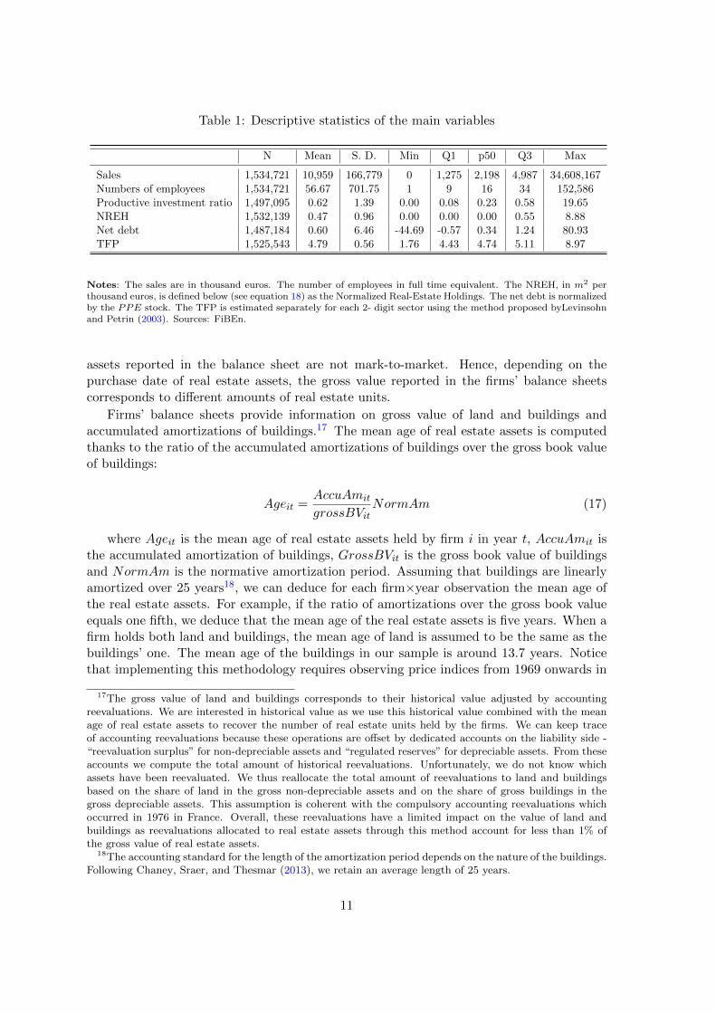
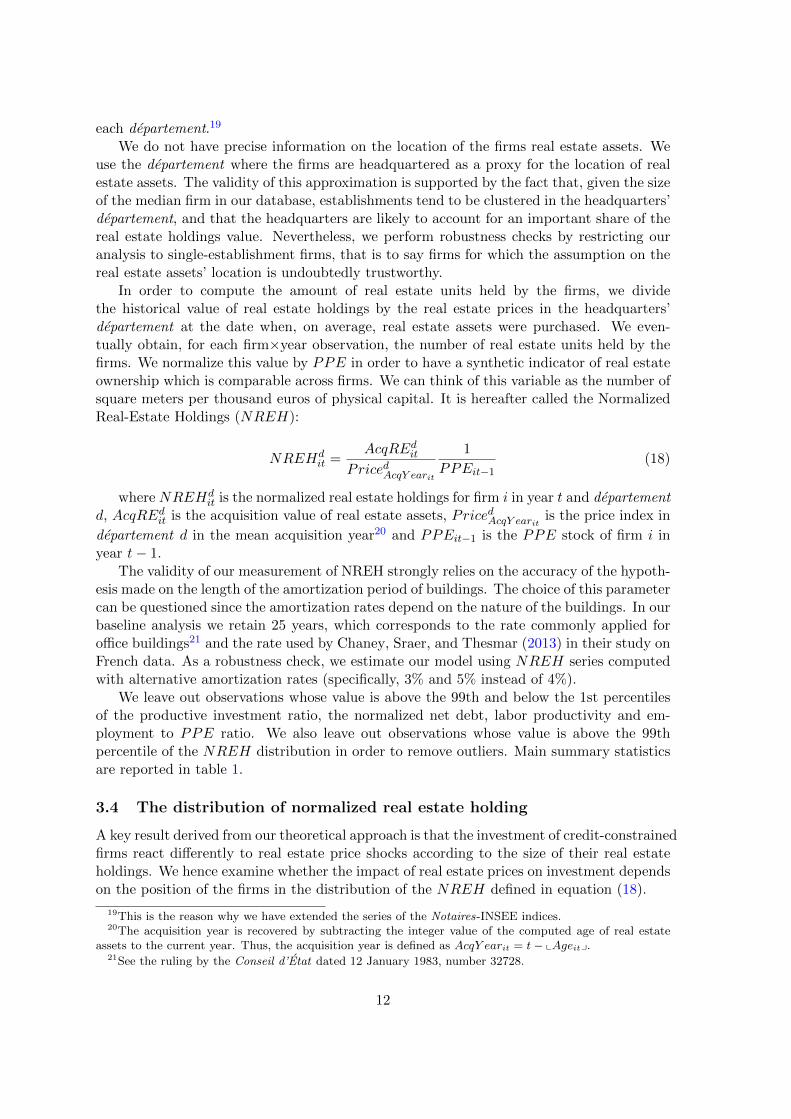
Table 1: Descriptive statistics of the main variables

N Mean S. D. Min Q1 p50 Q3 Max

Sales 1,534,721 10,959 166,779 0 1,275 2,198 4,987 34,608,167Numbers of employees 1,534,721 56.67 701.75 1 9 16 34 152,586Productive investment ratio 1,497,095 0.62 1.39 0.00 0.08 0.23 0.58 19.65NREH 1,532,139 0.47 0.96 0.00 0.00 0.00 0.55 8.88Net debt 1,487,184 0.60 6.46 -44.69 -0.57 0.34 1.24 80.93TFP 1,525,543 4.79 0.56 1.76 4.43 4.74 5.11 8.97

Notes: The sales are in thousand euros. The number of employees in full time equivalent. The NREH, in m2 perthousand euros, is defined below (see equation 18) as the Normalized Real-Estate Holdings. The net debt is normalizedby the PPE stock. The TFP is estimated separately for each 2- digit sector using the method proposed byLevinsohnand Petrin (2003). Sources: FiBEn.

assets reported in the balance sheet are not mark-to-market. Hence, depending on thepurchase date of real estate assets, the gross value reported in the firms’ balance sheetscorresponds to different amounts of real estate units.

Firms’ balance sheets provide information on gross value of land and buildings andaccumulated amortizations of buildings.17 The mean age of real estate assets is computedthanks to the ratio of the accumulated amortizations of buildings over the gross book valueof buildings:

Ageit =AccuAmit

grossBVitNormAm (17)

where Ageit is the mean age of real estate assets held by firm i in year t, AccuAmit isthe accumulated amortization of buildings, GrossBVit is the gross book value of buildingsand NormAm is the normative amortization period. Assuming that buildings are linearlyamortized over 25 years18, we can deduce for each firm×year observation the mean age ofthe real estate assets. For example, if the ratio of amortizations over the gross book valueequals one fifth, we deduce that the mean age of the real estate assets is five years. When afirm holds both land and buildings, the mean age of land is assumed to be the same as thebuildings’ one. The mean age of the buildings in our sample is around 13.7 years. Noticethat implementing this methodology requires observing price indices from 1969 onwards in

17The gross value of land and buildings corresponds to their historical value adjusted by accountingreevaluations. We are interested in historical value as we use this historical value combined with the meanage of real estate assets to recover the number of real estate units held by the firms. We can keep traceof accounting reevaluations because these operations are offset by dedicated accounts on the liability side -“reevaluation surplus” for non-depreciable assets and “regulated reserves” for depreciable assets. From theseaccounts we compute the total amount of historical reevaluations. Unfortunately, we do not know whichassets have been reevaluated. We thus reallocate the total amount of reevaluations to land and buildingsbased on the share of land in the gross non-depreciable assets and on the share of gross buildings in thegross depreciable assets. This assumption is coherent with the compulsory accounting reevaluations whichoccurred in 1976 in France. Overall, these reevaluations have a limited impact on the value of land andbuildings as reevaluations allocated to real estate assets through this method account for less than 1% ofthe gross value of real estate assets.

18The accounting standard for the length of the amortization period depends on the nature of the buildings.Following Chaney, Sraer, and Thesmar (2013), we retain an average length of 25 years.

11

each departement.19

We do not have precise information on the location of the firms real estate assets. Weuse the departement where the firms are headquartered as a proxy for the location of realestate assets. The validity of this approximation is supported by the fact that, given the sizeof the median firm in our database, establishments tend to be clustered in the headquarters’departement, and that the headquarters are likely to account for an important share of thereal estate holdings value. Nevertheless, we perform robustness checks by restricting ouranalysis to single-establishment firms, that is to say firms for which the assumption on thereal estate assets’ location is undoubtedly trustworthy.

In order to compute the amount of real estate units held by the firms, we dividethe historical value of real estate holdings by the real estate prices in the headquarters’departement at the date when, on average, real estate assets were purchased. We even-tually obtain, for each firm×year observation, the number of real estate units held by thefirms. We normalize this value by PPE in order to have a synthetic indicator of real estateownership which is comparable across firms. We can think of this variable as the number ofsquare meters per thousand euros of physical capital. It is hereafter called the NormalizedReal-Estate Holdings (NREH):

NREHdit =

AcqREditPricedAcqY earit

1

PPEit−1(18)

where NREHdit is the normalized real estate holdings for firm i in year t and departement

d, AcqREdit is the acquisition value of real estate assets, PricedAcqY earit is the price index in

departement d in the mean acquisition year20 and PPEit−1 is the PPE stock of firm i inyear t− 1.

The validity of our measurement of NREH strongly relies on the accuracy of the hypoth-esis made on the length of the amortization period of buildings. The choice of this parametercan be questioned since the amortization rates depend on the nature of the buildings. In ourbaseline analysis we retain 25 years, which corresponds to the rate commonly applied foroffice buildings21 and the rate used by Chaney, Sraer, and Thesmar (2013) in their study onFrench data. As a robustness check, we estimate our model using NREH series computedwith alternative amortization rates (specifically, 3% and 5% instead of 4%).

We leave out observations whose value is above the 99th and below the 1st percentilesof the productive investment ratio, the normalized net debt, labor productivity and em-ployment to PPE ratio. We also leave out observations whose value is above the 99thpercentile of the NREH distribution in order to remove outliers. Main summary statisticsare reported in table 1.

3.4 The distribution of normalized real estate holding

A key result derived from our theoretical approach is that the investment of credit-constrainedfirms react differently to real estate price shocks according to the size of their real estateholdings. We hence examine whether the impact of real estate prices on investment dependson the position of the firms in the distribution of the NREH defined in equation (18).

19This is the reason why we have extended the series of the Notaires-INSEE indices.20The acquisition year is recovered by subtracting the integer value of the computed age of real estate

assets to the current year. Thus, the acquisition year is defined as AcqY earit = t− xAgeity.21See the ruling by the Conseil d’Etat dated 12 January 1983, number 32728.

12

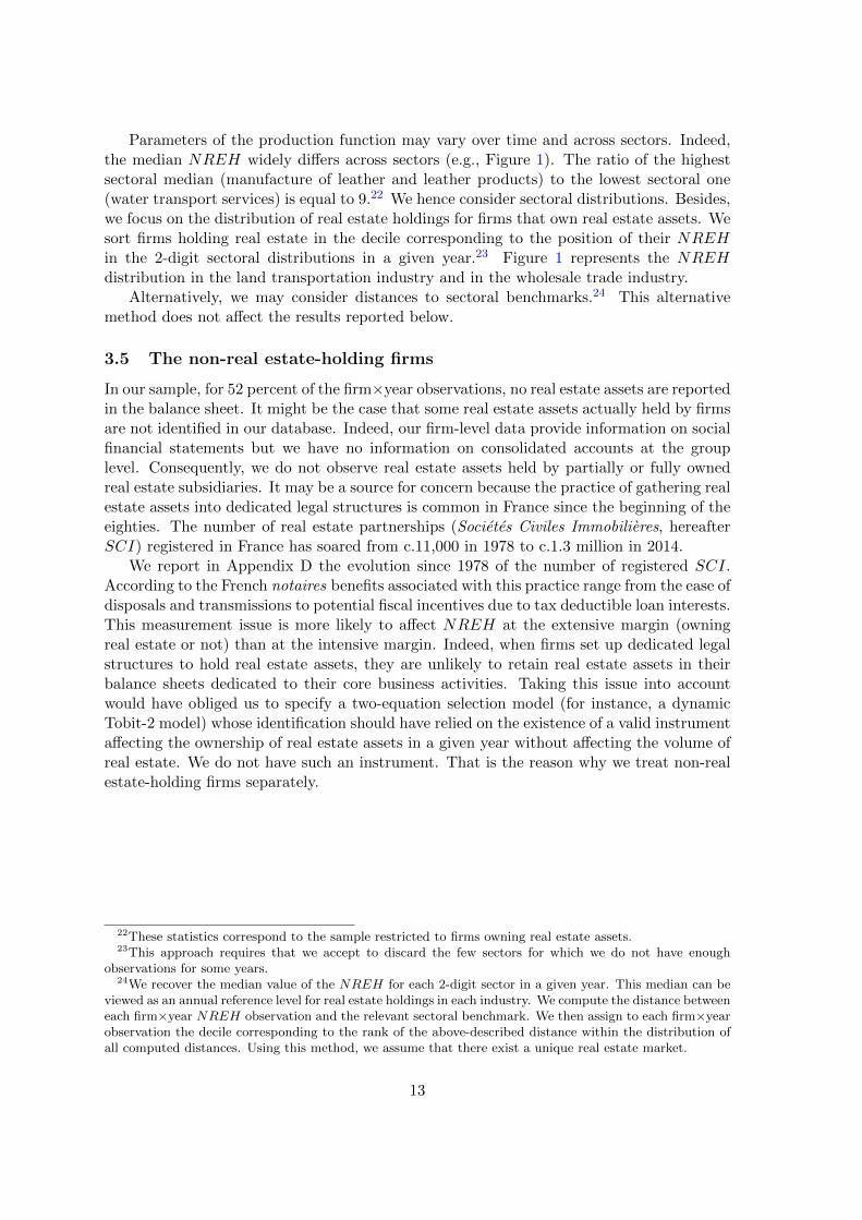
Parameters of the production function may vary over time and across sectors. Indeed,the median NREH widely differs across sectors (e.g., Figure 1). The ratio of the highestsectoral median (manufacture of leather and leather products) to the lowest sectoral one(water transport services) is equal to 9.22 We hence consider sectoral distributions. Besides,we focus on the distribution of real estate holdings for firms that own real estate assets. Wesort firms holding real estate in the decile corresponding to the position of their NREHin the 2-digit sectoral distributions in a given year.23 Figure 1 represents the NREHdistribution in the land transportation industry and in the wholesale trade industry.

Alternatively, we may consider distances to sectoral benchmarks.24 This alternativemethod does not affect the results reported below.

3.5 The non-real estate-holding firms

In our sample, for 52 percent of the firm×year observations, no real estate assets are reportedin the balance sheet. It might be the case that some real estate assets actually held by firmsare not identified in our database. Indeed, our firm-level data provide information on socialfinancial statements but we have no information on consolidated accounts at the grouplevel. Consequently, we do not observe real estate assets held by partially or fully ownedreal estate subsidiaries. It may be a source for concern because the practice of gathering realestate assets into dedicated legal structures is common in France since the beginning of theeighties. The number of real estate partnerships (Societes Civiles Immobilieres, hereafterSCI) registered in France has soared from c.11,000 in 1978 to c.1.3 million in 2014.

We report in Appendix D the evolution since 1978 of the number of registered SCI.According to the French notaires benefits associated with this practice range from the ease ofdisposals and transmissions to potential fiscal incentives due to tax deductible loan interests.This measurement issue is more likely to affect NREH at the extensive margin (owningreal estate or not) than at the intensive margin. Indeed, when firms set up dedicated legalstructures to hold real estate assets, they are unlikely to retain real estate assets in theirbalance sheets dedicated to their core business activities. Taking this issue into accountwould have obliged us to specify a two-equation selection model (for instance, a dynamicTobit-2 model) whose identification should have relied on the existence of a valid instrumentaffecting the ownership of real estate assets in a given year without affecting the volume ofreal estate. We do not have such an instrument. That is the reason why we treat non-realestate-holding firms separately.

22These statistics correspond to the sample restricted to firms owning real estate assets.23This approach requires that we accept to discard the few sectors for which we do not have enough

observations for some years.24We recover the median value of the NREH for each 2-digit sector in a given year. This median can be

viewed as an annual reference level for real estate holdings in each industry. We compute the distance betweeneach firm×year NREH observation and the relevant sectoral benchmark. We then assign to each firm×yearobservation the decile corresponding to the rank of the above-described distance within the distribution ofall computed distances. Using this method, we assume that there exist a unique real estate market.

13

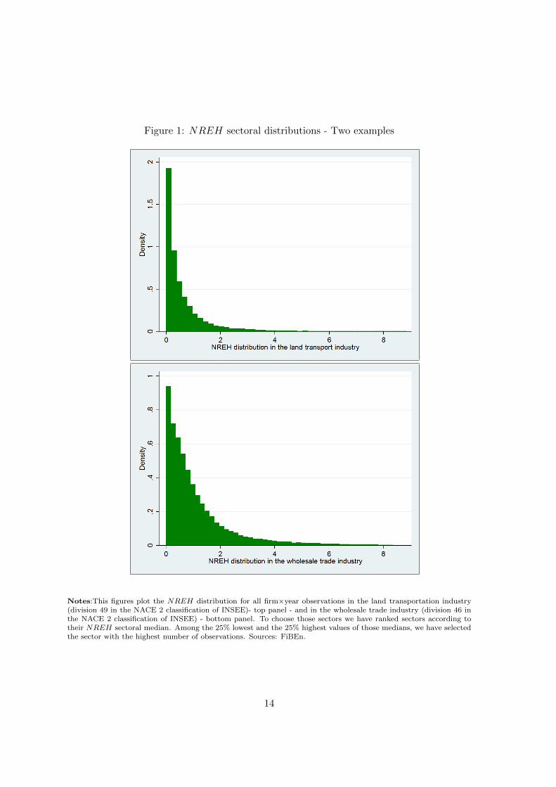
Figure 1: NREH sectoral distributions - Two examples

Notes:This figures plot the NREH distribution for all firm×year observations in the land transportation industry(division 49 in the NACE 2 classification of INSEE)- top panel - and in the wholesale trade industry (division 46 inthe NACE 2 classification of INSEE) - bottom panel. To choose those sectors we have ranked sectors according totheir NREH sectoral median. Among the 25% lowest and the 25% highest values of those medians, we have selectedthe sector with the highest number of observations. Sources: FiBEn.

14

4 The effects of real estate prices

We analyze the effect of real estate prices on corporate investment at the firm level. Ourempirical analysis is based on our theoretical model.

4.1 Estimating the investment equation

We first estimate the reduced-form equation (16) presented in section 2.4. More specifically,the estimated investment equation in year t for a firm i headquartered in departement d is:

Invit = αi + γt + β1NREHdit−1 + β2lnPrice

dt + β3NetDebtit−1 + β4TFPit−1 + εit (19)

where:

• Invit is firm’s i capital expenditure net of real estate acquisitions normalized by thePPE stock in period t− 1;

• NREHdit−1 is the number of real estate units held by firm i at the end of year t− 1,

normalized by the PPE stock in period t− 1 as defined in equation 18;

• lnPricedt is the logarithm of the real estate transaction price per square meter indepartement d in year t;

• NetDebtit−1 is firm’s i total financial debt minus cash holdings of firm i at the end ofyear t− 1 normalized by the PPE stock in period t− 1;

• TFPit−1 is firm’s i total factor of productivity in t−1 estimated by using the methodintroduced by Levinsohn and Petrin (2003);

As suggested by our theoretical framework, we aggregate financial debt and cash hold-ings.25 We include firms fixed-effects (hereafter, FE), which are assumed to control for allthe time invariant unobserved firms’ characteristics, and year dummies which control foreconomic conditions at the aggregate level. We allow for possible correlations between theshocks εit at the departement×year level.26

To validate empirically the theoretical prediction regarding the effect of real estate priceson corporate investment, we allow real estate prices to have differentiated effects dependingon the firms’ position in the NREH distribution. For that purpose, we introduce interactionterms between real estate prices and NREH deciles. We estimate the following equation:

25Besides, this specification allows to take into account the fact that firms may contract loans to financeinvestment in the accounting period preceding the investment. In that case, an increase in the financialdebt will be positively correlated with investment in the subsequent period. It may hide the fact that higherleverages lessen firms’ capacity to finance investment. Aggregating financial debt and cash holdings is aneasy way to overcome this issue. Indeed, if proceeds from the loans are not used to finance investment inthe contemporaneous accounting period, they will inflate cash holdings and have no impact on the net debt(computed as the financial debt minus the cash).

26Interpretations of β1, β2, β3 and β4 are derived from the model. The coefficient β1 is expected tobe positive if the sample contains constrained firms. It reflects the fact that constrained firms can relaxtheir borrowing constraint through real estate assets pledging. As shown in section 2, the coefficient β2 isexpected to be negative for unconstrained firms and to depend on the amount of real estate units held bythe constrained firms. The coefficient β3 is also expected to be negative if the sample contains constrainedfirms. The coefficient β4 is expected to be positive.

15

Invit = αi + γt + β1NREHdit−1 +

∑10j=1 β

j2D

j

it−1lP ricedt +

∑10j=1 λjD

j

it−1

+β3NetDebtit−1 + β4TFP it−1 + εit(20)

where Dj

it−1 for i = 1, ..., 10 is a dummy variable indicating if the firms’ NREH belongsto the i-th decile of the distribution.

We report in Table 2 parameter estimates of equation (19). Column 1 corresponds tothe OLS estimation of equation (19). The parameter estimates associated with the NREHis found to be positive. The baseline coefficient is 0.12, meaning that one additional squaremeter increases, on average, yearly investment by 120 euros. The estimated coefficientassociated with net debt is negative: each additional 1 euro of net debt decreases yearlyinvestment by 0.6 cent. The coefficient associated with productivity is positive. Thesecoefficients are all statistically significant at the 1 percent level. The estimated coefficientassociated with real estate prices is positive but not significant. Those estimates are con-sistent with the predictions derived from our theoretical framework. Column 2 correspondsto the same estimation with year dummies. Introducing year dummies affects the coeffi-cient associated with real estate prices which now becomes statistically significant at the5% level. On average, a 10% increase in real estate price translates into a 0.35 percentagepoint increase in the investment ratio; that corresponds to 1.5% of the median investmentratio. Other coefficients remain largely unaffected. Column 3 corresponds to the sameestimation with year×sector dummies. Sectoral dynamics at the aggregate level may affectthe path of corporate investment; these sectoral shocks are captured by the year×sectordummies. The coefficients remain unchanged. Column 4 reports parameter estimates ofequation (19) for single-establishment firms. The assumption made on the location of realestate assets (the departement where the firms are headquartered) is strong. Nevertheless,it is unquestionably true for firms operating only in one establishment. Splitting the sam-ple between multiple and single-establishment firms allows to appraise the importance ofthis assumption. Estimates of the coefficients are largely unaffected when we restrict thesample to single-establishment firms. Columns 5 and 6 explore firms’ behavior dependingon their size; they present parameter estimates of equation (19) for small and large firms,respectively. Small firms are defined as firms reporting, in the initial observation year, arevenue below the 25th percentile of revenues in the corresponding year, and large firmsare the ones reporting an initial revenue above the 75th percentile. The estimate coefficientassociated with NREH is higher for small firms than for large firms, and statistically sig-nificant at the 1 percent level for both samples. Small firms being more likely to be creditconstrained than large firms, this result is perfectly in line with our theoretical predictions.Also in accordance with our expectations, the absolute value of the estimated coefficientassociated with net debt is higher for small firms. The estimated coefficient associated withreal estate prices is positive and statistically significant at the 1 percent level for large firms,and negative and not significant for small firms. The effects of real estate prices appear tobe heterogeneous.

As mentioned above, the group made of non-real estate-holding firms includes also firmsthat might own some real estate assets through subsidiaries. Heterogeneity among thisgroup may bias our estimates. We hence present in Table 3 the same estimates for thesubsample of firms holding real estate assets.

To elaborate on heterogeneous effects of prices on corporate investment, we estimateequation (20) and report the results in Table 4.

16

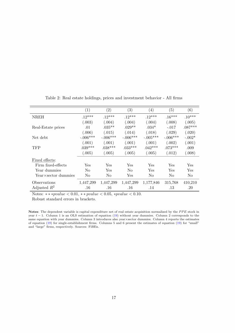
Table 2: Real estate holdings, prices and investment behavior - All firms

(1) (2) (3) (4) (5) (6)

NREH .12*** .12*** .12*** .12*** .16*** .10***(.003) (.004) (.004) (.004) (.008) (.005)

Real-Estate prices .01 .035** .029** .034* -.017 .087***(.006) (.015) (.014) (.018) (.029) (.020)

Net debt -.006*** -.006*** -.006*** -.005*** -.006*** -.002*(.001) (.001) (.001) (.001) (.002) (.001)

TFP .039*** .038*** .033*** .042*** .073*** .009(.005) (.005) (.005) (.005) (.012) (.008)

Fixed effects:Firm fixed-effects Yes Yes Yes Yes Yes YesYear dummies No Yes No Yes Yes YesYear×sector dummies No No Yes No No No

Observations 1,447,299 1,447,299 1,447,299 1,177,846 315,768 410,210Adjusted R2 .16 .16 .16 .14 .13 .20

Notes: ∗ ∗ ∗pvalue < 0.01, ∗ ∗ pvalue < 0.05, ∗pvalue < 0.10.Robust standard errors in brackets.

Notes: The dependent variable is capital expenditure net of real estate acquisition normalized by the PPE stock inyear t − 1. Column 1 is an OLS estimation of equation (19) without year dummies. Column 2 corresponds to thesame equation with year dummies. Column 3 introduces also year×sector dummies. Column 4 reports the estimatesof equation (19) for single-establishment firms. Columns 5 and 6 present the estimates of equation (19) for “small”and “large” firms, respectively. Sources: FiBEn.

17

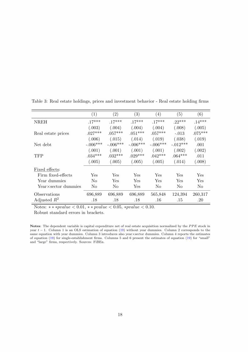
Table 3: Real estate holdings, prices and investment behavior - Real estate holding firms

(1) (2) (3) (4) (5) (6)

NREH .17*** .17*** .17*** .17*** .22*** .14***(.003) (.004) (.004) (.004) (.008) (.005)

Real estate prices .027*** .057*** .051*** .057*** -.013 .075***(.006) (.015) (.014) (.019) (.038) (.019)

Net debt -.006*** -.006*** -.006*** -.006*** -.012*** .001(.001) (.001) (.001) (.001) (.002) (.002)

TFP .034*** .032*** .029*** .042*** .064*** .011(.005) (.005) (.005) (.005) (.014) (.008)

Fixed effects:Firm fixed-effects Yes Yes Yes Yes Yes YesYear dummies No Yes Yes Yes Yes YesYear×sector dummies No No Yes No No No

Observations 696,889 696,889 696,889 565,848 124,394 260,317Adjusted R2 .18 .18 .18 .16 .15 .20



18

Table 4: Real estate holdings, prices and investment behavior - Heterogeneous effects bydeciles of real estate holding

(1) (2) (3) (4) (5) (6)

NREH .11*** .11*** .11*** .11*** .13*** .10***(.005) (.005) (.005) (.005) (.012) (.007)

Real estate prices -.14*** -.048*** -.052*** -.073*** -.13*** -.013(.015) (.018) (.018) (.022) (.046) (.028)

Real estate prices×dec2 .043*** .046*** .046*** .059*** .081** .032(.016) (.016) (.016) (.016) (.035) (.030)

Real estate prices×dec3 .035** .04** .041** .051*** .048 .032(.018) (.018) (.018) (.017) (.035) (.030)

Real estate prices×dec4 .056*** .063*** .063*** .089*** .10** .053*(.018) (.018) (.018) (.018) (.040) (.030)

Real estate prices×dec5 .094*** .10*** .10*** .11*** .090** .091***(.019) (.019) (.019) (.018) (.036) (.030)

Real estate prices×dec6 .12*** .13*** .13*** .14*** .14*** .096***(.019) (.018) (.018) (.018) (.036) (.028)





Net debt -.006*** -.006*** -.006*** -.006*** -.012*** .001(.001) (.001) (.001) (.001) (.003) (.002)

TFP .032*** .034*** .032*** .043*** .063*** .014*(.005) (.005) (.005) (.005) (.014) (.008)

Fixed effects:Decile dummies Yes Yes Yes Yes Yes YesFirm fixed-effects Yes Yes Yes Yes Yes YesYear dummies No Yes Yes Yes Yes YesYear×sector dummies No No Yes No No No

Observations 696,599 696,599 696,599 565,612 124,344 260,218Adjusted R2 .18 .18 .18 .17 .16 .20

Notes: ∗ ∗ ∗pvalue < 0.01. ∗ ∗ pvalue < 0.05. ∗pvalue < 0.10.Robust standard errors in brackets.


19

Column 1 reports OLS parameter estimates of equation (20) without year fixed effects.The coefficients associated with interactions between real estate prices and deciles of thesectoralNREH distribution exhibit a pattern which is very much in line with our theoreticalresults. We observe a monotonic increase in the estimated values, going from negative valuesfor the lowest decile to high positive values for the highest ones. While the investment offirms that have few real estate holdings compared to their sectoral peers is slightly negativelyaffected by an increase in real estate prices, the investment of those holding more realestate, relatively to their peers, is very significantly and positively impacted by increasingreal estate prices. Estimated values of the coefficient associated with the other regressorsremain largely unaffected by the introduction of interactions between real estate prices andNREH deciles into the list of regressors. Column 2 corresponds to the same estimationwith year fixed effects. In column 3, we add year×sector fixed effects. Parameter estimatesare similar for these three specifications. Results from our preferred estimation (column 2)imply that a 10% increase in real estate prices causes a 0.48 percentage point decrease inthe investment rate of firms belonging to the first decile of the NREH distribution, that isto say approximately 1% of the mean investment rate in the first NREH decile, but a 3.1percentage point increase in the investment rate of firms belonging to the last decile, that isto say approximately 6% of the mean investment rate in the top NREH decile. In column4, we present estimated parameters of equation (20) for single-establishment firms only.Estimates are similar to those obtained for the whole sample (column 2, Table 4) except forthe estimated parameter associated with the interaction terms between real estate pricesand the lowest NREH deciles. These results echo estimates reported in columns 5 and 6which present estimates of the same equation for small and large firms, respectively. Thenegative effect of real estate price increases on the investment rate of firms located in thefirst deciles of the NREH distribution is much higher for small firms than for large firms.This could result from differences in the intensity of the borrowing constraint of small andlarge firms. Moreover, there may be concern that the increase in the estimated coefficientsassociated with the interaction terms could result from the variability of firms’ size acrossdeciles. The fact that we find the same patterns of results for both sub-samples (namely,small and large firms) gives credence to the idea that it is mainly the intensity in real estateholding, namely the NREH value, that matters for predicting the effect of real estate priceson firms’ productive investment.

Let us examine now the effect of real estate prices on the productive investment ofnon-real estate-holding firms.

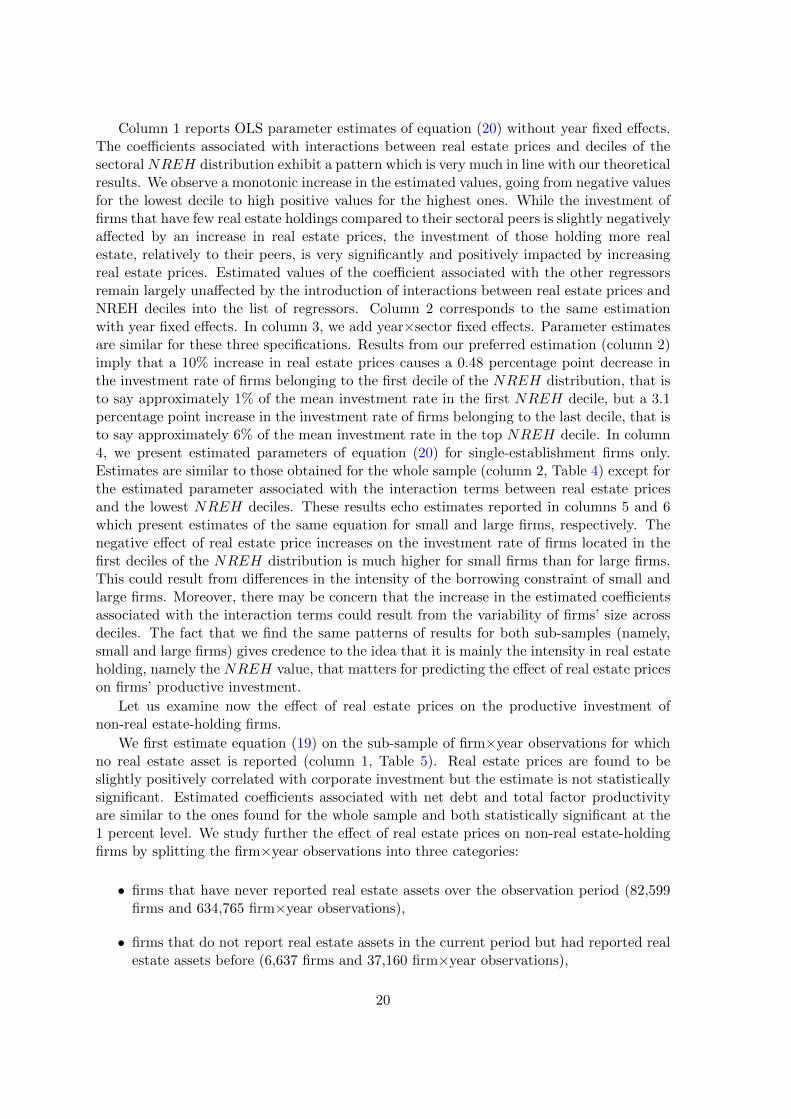
We first estimate equation (19) on the sub-sample of firm×year observations for whichno real estate asset is reported (column 1, Table 5). Real estate prices are found to beslightly positively correlated with corporate investment but the estimate is not statisticallysignificant. Estimated coefficients associated with net debt and total factor productivityare similar to the ones found for the whole sample and both statistically significant at the1 percent level. We study further the effect of real estate prices on non-real estate-holdingfirms by splitting the firm×year observations into three categories:

• firms that have never reported real estate assets over the observation period (82,599firms and 634,765 firm×year observations),

• firms that do not report real estate assets in the current period but had reported realestate assets before (6,637 firms and 37,160 firm×year observations),

20

Table 5: Real estate prices and investment behavior - Results no real estate firms

(1) (2) (3) (4) (5)

Real estate prices .012 .031 .001 -.18* -.54*(.023) (.025) (.09) (.11) (.31)

Net debt -.006*** -.006*** -.013*** -.010** -.021***(.001) (.001) (.003) (.004) (.008)

TFP .067*** .064*** .094*** .053* .17***(.008) (.008) (.035) (.029) (.064)

Fixed effects:Firm fixed-effects Yes Yes Yes Yes YesYear dummies Yes Yes Yes Yes Yes

Observations 750,410 634,765 37,160 73,259 37,351Adjusted R2 .15 .14 .18 .20 .18


Notes: The dependent variable is capital expenditure net of real estate acquisition normalized by the PPE stockin year t − 1. Column 1 reports estimates from the sample made of firm×year observations for which no real estateassets are reported. Column 2 corresponds to the same estimation on the sub-sample made of firms that have neverheld real estate. Column 3 and 4 correspond to firms that don’t report real estate assets in contemporaneous periodbut have reported real estate before (column 3) or after (column 4). In column 5, we restrict the analysis to the 3years preceding the acquisition. Sources: FiBEn.

21

• firms that do not report real estate assets in the current period but will acquire realestate assets afterward (15,598 firms and 73,259 firm×year observations).

Results are presented in columns 2, 3 and 4 of Table 5, respectively. We observe that realestate prices do not significantly affect productive investment of the first two categories buthave a negative impact, statistically significant at the 10 percent level, on the last category.This negative effect of real estate prices on firms’ investment is more pronounced if werestrict the analysis to the three years preceding real estate acquisition (column 5, Table 5).These results tend to show that non-real estate-holding firms are rather immune from realestate prices when they are not considering real estate acquisitions. The negative effect ofan increase in real estate prices on capital investment could result from a crowding-out effectof planned real estate investment on current productive investments. These results can bealternatively explained by the above-mentioned measurement issue. More precisely, firmsthat initially report no real estate holdings and that, at some point in time, start reportingreal estate assets on their balance sheet are unlikely to be involved in the legal separation ofreal estate holdings prior to the acquisition. Hence, even if the legal separation of real estateholdings blurs the effects of real estate prices for seemingly non-real estate-holding firms,we nevertheless expect that real estate prices have a negative impact on the investment offirms that report no real estate assets in the current period but acquire some later.

4.2 Complementary robustness checks

We have identified varying effects of real estate prices on corporate investment depending onthe position of the firms in the NREH sectoral distributions. However, these results couldbe biased if real estate holdings were correlated with the sensitivity of investment to localreal estate prices. For example, we would overestimate the effect of real estate prices oninvestment for real estate-rich firm if those firms were more sensitive to the local economiccondition. This issue of the sensitivity to local economic condition is partly addressed bythe consideration of sectoral distributions for the variable NREH. Nevertheless, we canrefine our analysis by introducing interaction terms between real estate prices and age,size or profit margin of the firm in equation (20). Indeed, if age, size or profitability arecorrelated with firms’ real estate holdings as well as with firms’ sensitivity to local economicconditions, the introduction of those interaction terms is required to properly identify theimpact of real estate prices. The estimation results corresponding to this specification arepresented in column 2 in Table 6 whereas column 1 reports our baseline estimates presentedin column 2 in Table 20. Our results are largely unaffected by the introduction of theseinteractions terms.

Another possible cause for concern could be that firms invest in real estate asset prior toinvesting in productive assets entailing a spurious correlation, possibly varying with the levelof real estate prices, between real estate holdings and subsequent productive investment. Inorder to ensure that this mechanism doesn’t affect our results, we present estimation resultsof equation (20) with lagged values for real estate holdings (3 and 4 years, respectively) incolumn 2 and 3 in Table 6. These alternative specifications tend to alter the precision of ourestimates associated with interacted prices even if we still obtain the same upward trend.

As mentioned above, real estate prices are likely to be correlated with local investmentopportunities. Our empirical strategy relies on the comparison of the investment of firmsfacing the same local economic conditions but varying exposition to real estate prices be-cause of different real estate holdings. The efficiency of this difference-in-difference strategy

22

in disentangling the effects of real estate prices on investment from the impact of local eco-nomic impetus can be assessed by stratifying firms belonging to tradable and non-tradablesectors. Indeed, firms operating in tradable sectors are less affected by local economic con-dition while they are similarly affected by the profit and the collateral channels followingreal estate prices’ fluctuations. The estimation results of equation (20) for firms operat-ing in tradable sectors are presented in column 4 of Table 6, results for firms operatingin non-tradable sectors are presented in column 5. The sign and the magnitude of theestimates associated with prices are similar in the two sub-samples. We also would liketo account for other local economic variables likely to affect corporate investment and tocorrelate with real estate prices. Local unemployment rate at the departement ’s level areproduced by the INSEE for the whole period studied. We estimate equation (20) adding avariable corresponding to the local unemployment rate in the departement where the firm iis headquartered in year t. The results are reported in column 7 in Table 6. We obtain anexpected negative and statistically significant estimate for the coefficient associated withthe local unemployment. The other estimates are not altered by the introduction of thiscontrol.27

We do not tackle the issue of attrition because we do not have precise information onthe reasons why firms enter or exit the sample. Nevertheless, to ensure that the movesin and out of the sample do not affect our results, we estimate our preferred equation(column 1, Table 7), on a balanced panel in which firms are observed each year from 1994onwards. Results are reported in column 2, Table 7. Our findings concerning the impactof prices are robust to this restriction. In columns 3 and 4, we present the results of ourbaseline estimation conducted on two subperiods of equal length, 1994-2003 and 2004-2013,respectively. The estimate associated with the NREH variable increases during the secondhalf of the observation period, which suggests that firms may have faced fiercer creditconstraint during this subperiod. Columns 5 and 6 report the results obtained when theamortization rate used to build NREH series is 3% and 5% per year, respectively, insteadof 4% per year in our baseline estimation. The estimates are unaffected, except for thecoefficient associated with the NREH variable. This coefficient mechanically increases withthe depreciation rate as, in a context of an overall sharp increase in real estate prices, theolder the acquisition date the higher the proxied real estate volume. Column 7 correspondsto the subsample without firms headquartered in Ile-de-France (Paris region) which appearsto be an outlier with respect to real estate prices evolution (see Figure 2 in Appendix C).Column 8 shows that considering an alternative measure of TFP, that is to say residualsfrom simple OLS regression at 2-digit level, has no impact on our results.

4.3 The borrowing capacity channel and other real effects of real estateprices

In our model, the effect of real estate prices on productive investment of constrained firmsis channeled through changes in the firms’ borrowing capacity; for unconstrained firms, realestate prices may also affect (negatively) the level of debt if investment is not internallyfinanced. Hence, we should observe similar results with regards to the impact of the differentexplanatory variables on investment and on new bank loans. Unfortunately, the balancesheet data do not provide information on the new bank loans. We only observe the amount

27In unreported regressions, we find that when we interact local unemployment with the NREH deciles,none of the coefficient associated with the interacted terms is statistically significant.

23

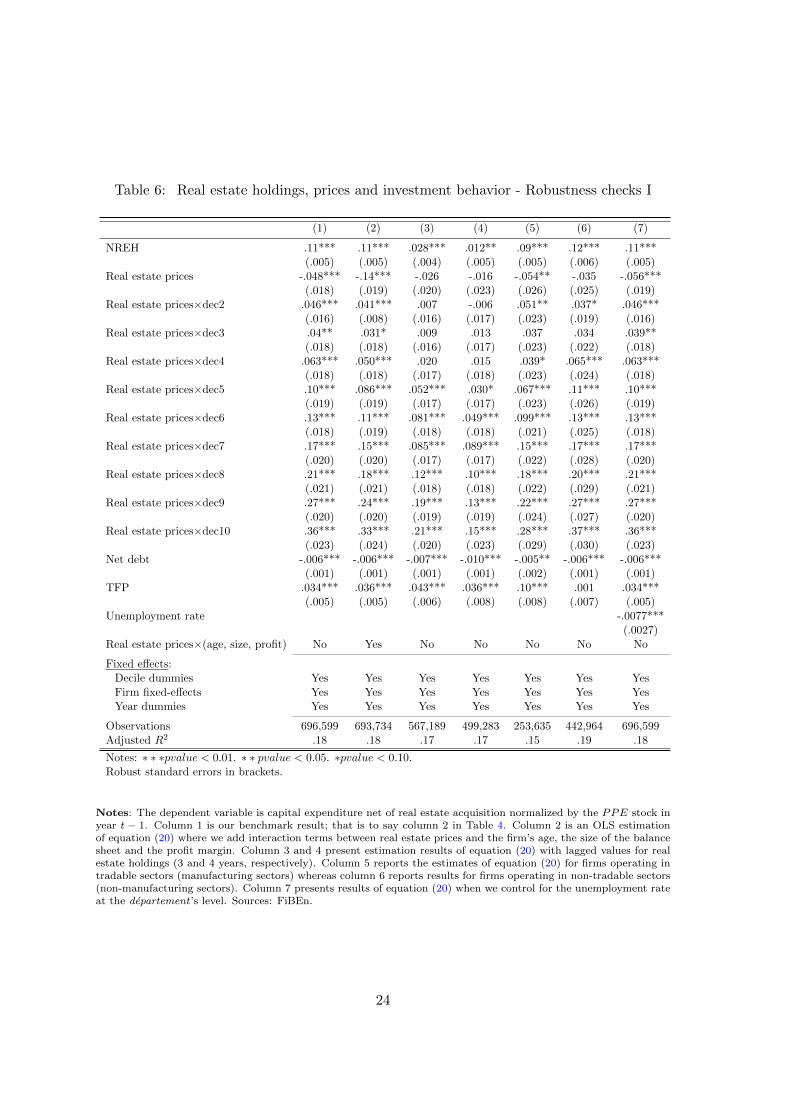
Table 6: Real estate holdings, prices and investment behavior - Robustness checks I

(1) (2) (3) (4) (5) (6) (7)

NREH .11*** .11*** .028*** .012** .09*** .12*** .11***(.005) (.005) (.004) (.005) (.005) (.006) (.005)

Real estate prices -.048*** -.14*** -.026 -.016 -.054** -.035 -.056***(.018) (.019) (.020) (.023) (.026) (.025) (.019)

Real estate prices×dec2 .046*** .041*** .007 -.006 .051** .037* .046***(.016) (.008) (.016) (.017) (.023) (.019) (.016)

Real estate prices×dec3 .04** .031* .009 .013 .037 .034 .039**(.018) (.018) (.016) (.017) (.023) (.022) (.018)

Real estate prices×dec4 .063*** .050*** .020 .015 .039* .065*** .063***(.018) (.018) (.017) (.018) (.023) (.024) (.018)

Real estate prices×dec5 .10*** .086*** .052*** .030* .067*** .11*** .10***(.019) (.019) (.017) (.017) (.023) (.026) (.019)

Real estate prices×dec6 .13*** .11*** .081*** .049*** .099*** .13*** .13***(.018) (.019) (.018) (.018) (.021) (.025) (.018)





Net debt -.006*** -.006*** -.007*** -.010*** -.005** -.006*** -.006***(.001) (.001) (.001) (.001) (.002) (.001) (.001)

TFP .034*** .036*** .043*** .036*** .10*** .001 .034***(.005) (.005) (.006) (.008) (.008) (.007) (.005)

Unemployment rate -.0077***(.0027)

Real estate prices×(age, size, profit) No Yes No No No No No

Fixed effects:Decile dummies Yes Yes Yes Yes Yes Yes YesFirm fixed-effects Yes Yes Yes Yes Yes Yes YesYear dummies Yes Yes Yes Yes Yes Yes Yes

Observations 696,599 693,734 567,189 499,283 253,635 442,964 696,599Adjusted R2 .18 .18 .17 .17 .15 .19 .18


Notes: The dependent variable is capital expenditure net of real estate acquisition normalized by the PPE stock inyear t − 1. Column 1 is our benchmark result; that is to say column 2 in Table 4. Column 2 is an OLS estimationof equation (20) where we add interaction terms between real estate prices and the firm’s age, the size of the balancesheet and the profit margin. Column 3 and 4 present estimation results of equation (20) with lagged values for realestate holdings (3 and 4 years, respectively). Column 5 reports the estimates of equation (20) for firms operating intradable sectors (manufacturing sectors) whereas column 6 reports results for firms operating in non-tradable sectors(non-manufacturing sectors). Column 7 presents results of equation (20) when we control for the unemployment rateat the departement ’s level. Sources: FiBEn.

24

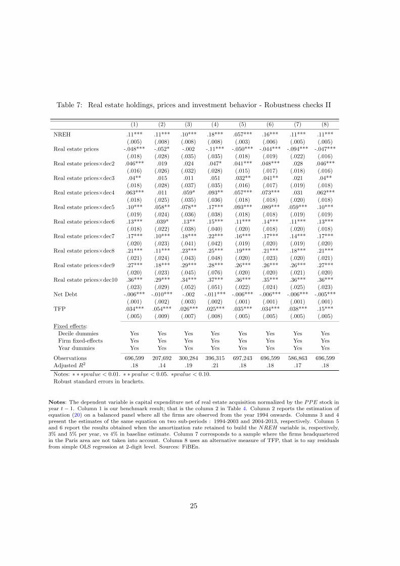
Table 7: Real estate holdings, prices and investment behavior - Robustness checks II

(1) (2) (3) (4) (5) (6) (7) (8)

NREH .11*** .11*** .10*** .18*** .057*** .16*** .11*** .11***(.005) (.008) (.008) (.008) (.003) (.006) (.005) (.005)

Real estate prices -.048*** -.052* -.002 -.11*** -.050*** -.044*** -.094*** -.047***(.018) (.028) (.035) (.035) (.018) (.019) (.022) (.016)

Real estate prices×dec2 .046*** .019 .024 .047* .041*** .048*** .028 .046***(.016) (.026) (.032) (.028) (.015) (.017) (.018) (.016)

Real estate prices×dec3 .04** .015 .011 .051 .032** .041** .021 .04**(.018) (.028) (.037) (.035) (.016) (.017) (.019) (.018)

Real estate prices×dec4 .063*** .011 .059* .093** .057*** .073*** .031 .062***(.018) (.025) (.035) (.036) (.018) (.018) (.020) (.018)

Real estate prices×dec5 .10*** .058** .078** .17*** .093*** .089*** .059*** .10***(.019) (.024) (.036) (.038) (.018) (.018) (.019) (.019)

Real estate prices×dec6 .13*** .039* .13** .15*** .11*** .14*** .11*** .13***(.018) (.022) (.038) (.040) (.020) (.018) (.020) (.018)

Real estate prices×dec7 .17*** .10*** .18*** .22*** .16*** .17*** .14*** .17***(.020) (.023) (.041) (.042) (.019) (.020) (.019) (.020)




Net Debt -.006*** -.010*** -.002 -.011*** -.006*** -.006*** -.006*** -.005***(.001) (.002) (.003) (.002) (.001) (.001) (.001) (.001)

TFP .034*** .054*** .026*** .025*** .035*** .034*** .038*** .15***(.005) (.009) (.007) (.008) (.005) (.005) (.005) (.005)

Fixed effects:Decile dummies Yes Yes Yes Yes Yes Yes Yes YesFirm fixed-effects Yes Yes Yes Yes Yes Yes Yes YesYear dummies Yes Yes Yes Yes Yes Yes Yes Yes

Observations 696,599 207,692 300,284 396,315 697,243 696,599 586,863 696,599Adjusted R2 .18 .14 .19 .21 .18 .18 .17 .18


Notes: The dependent variable is capital expenditure net of real estate acquisition normalized by the PPE stock inyear t − 1. Column 1 is our benchmark result; that is the column 2 in Table 4. Column 2 reports the estimation ofequation (20) on a balanced panel where all the firms are observed from the year 1994 onwards. Columns 3 and 4present the estimates of the same equation on two sub-periods : 1994-2003 and 2004-2013, respectively. Column 5and 6 report the results obtained when the amortization rate retained to build the NREH variable is, respectively,3% and 5% per year, vs 4% in baseline estimate. Column 7 corresponds to a sample where the firms headquarteredin the Paris area are not taken into account. Column 8 uses an alternative measure of TFP, that is to say residualsfrom simple OLS regression at 2-digit level. Sources: FiBEn.

25

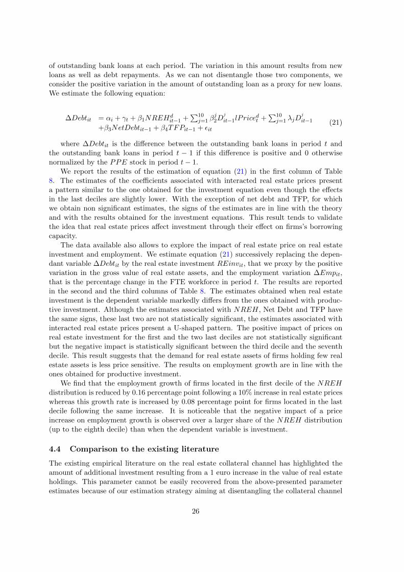
of outstanding bank loans at each period. The variation in this amount results from newloans as well as debt repayments. As we can not disentangle those two components, weconsider the positive variation in the amount of outstanding loan as a proxy for new loans.We estimate the following equation:

∆Debtit = αi + γt + β1NREHdit−1 +

∑10j=1 β

j2D

j

it−1lP ricedt +

∑10j=1 λjD

j

it−1

+β3NetDebtit−1 + β4TFPit−1 + εit(21)

where ∆Debtit is the difference between the outstanding bank loans in period t andthe outstanding bank loans in period t − 1 if this difference is positive and 0 otherwisenormalized by the PPE stock in period t− 1.

We report the results of the estimation of equation (21) in the first column of Table8. The estimates of the coefficients associated with interacted real estate prices presenta pattern similar to the one obtained for the investment equation even though the effectsin the last deciles are slightly lower. With the exception of net debt and TFP, for whichwe obtain non significant estimates, the signs of the estimates are in line with the theoryand with the results obtained for the investment equations. This result tends to validatethe idea that real estate prices affect investment through their effect on firms’s borrowingcapacity.

The data available also allows to explore the impact of real estate price on real estateinvestment and employment. We estimate equation (21) successively replacing the depen-dant variable ∆Debtit by the real estate investment REinvit, that we proxy by the positivevariation in the gross value of real estate assets, and the employment variation ∆Empit,that is the percentage change in the FTE workforce in period t. The results are reportedin the second and the third columns of Table 8. The estimates obtained when real estateinvestment is the dependent variable markedly differs from the ones obtained with produc-tive investment. Although the estimates associated with NREH, Net Debt and TFP havethe same signs, these last two are not statistically significant, the estimates associated withinteracted real estate prices present a U-shaped pattern. The positive impact of prices onreal estate investment for the first and the two last deciles are not statistically significantbut the negative impact is statistically significant between the third decile and the seventhdecile. This result suggests that the demand for real estate assets of firms holding few realestate assets is less price sensitive. The results on employment growth are in line with theones obtained for productive investment.

We find that the employment growth of firms located in the first decile of the NREHdistribution is reduced by 0.16 percentage point following a 10% increase in real estate priceswhereas this growth rate is increased by 0.08 percentage point for firms located in the lastdecile following the same increase. It is noticeable that the negative impact of a priceincrease on employment growth is observed over a larger share of the NREH distribution(up to the eighth decile) than when the dependent variable is investment.

4.4 Comparison to the existing literature

The existing empirical literature on the real estate collateral channel has highlighted theamount of additional investment resulting from a 1 euro increase in the value of real estateholdings. This parameter cannot be easily recovered from the above-presented parameterestimates because of our estimation strategy aiming at disentangling the collateral channel

26

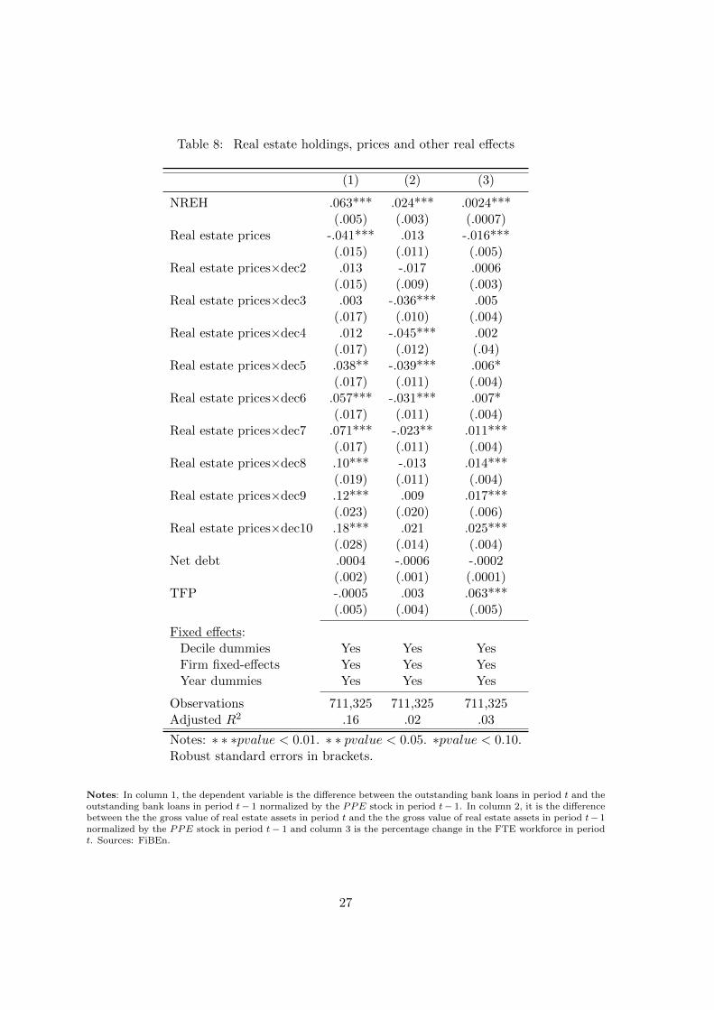
Table 8: Real estate holdings, prices and other real effects

(1) (2) (3)

NREH .063*** .024*** .0024***(.005) (.003) (.0007)

Real estate prices -.041*** .013 -.016***(.015) (.011) (.005)

Real estate prices×dec2 .013 -.017 .0006(.015) (.009) (.003)

Real estate prices×dec3 .003 -.036*** .005(.017) (.010) (.004)

Real estate prices×dec4 .012 -.045*** .002(.017) (.012) (.04)

Real estate prices×dec5 .038** -.039*** .006*(.017) (.011) (.004)

Real estate prices×dec6 .057*** -.031*** .007*(.017) (.011) (.004)

Real estate prices×dec7 .071*** -.023** .011***(.017) (.011) (.004)

Real estate prices×dec8 .10*** -.013 .014***(.019) (.011) (.004)

Real estate prices×dec9 .12*** .009 .017***(.023) (.020) (.006)

Real estate prices×dec10 .18*** .021 .025***(.028) (.014) (.004)

Net debt .0004 -.0006 -.0002(.002) (.001) (.0001)

TFP -.0005 .003 .063***(.005) (.004) (.005)

Fixed effects:Decile dummies Yes Yes YesFirm fixed-effects Yes Yes YesYear dummies Yes Yes Yes

Observations 711,325 711,325 711,325Adjusted R2 .16 .02 .03


Notes: In column 1, the dependent variable is the difference between the outstanding bank loans in period t and theoutstanding bank loans in period t− 1 normalized by the PPE stock in period t− 1. In column 2, it is the differencebetween the the gross value of real estate assets in period t and the the gross value of real estate assets in period t− 1normalized by the PPE stock in period t− 1 and column 3 is the percentage change in the FTE workforce in periodt. Sources: FiBEn.

27

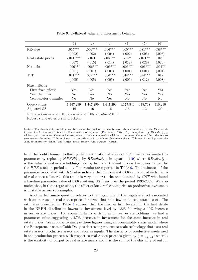
Table 9: Collateral value and investment behavior

(1) (2) (3) (4) (5) (6)

REvalue .065*** .066*** .066*** .065*** .081*** .058***(.002) (.002) (.004) (.002) (.005) (.003)

Real estate prices -.041 *** -.021 -.030** -.022 -.071** .023(.007) (.015) (.014) (.018) (.029) (.020)

Net debt -.006*** -.006*** -.005*** -.005*** -.006*** -.002**(.001) (.001) (.001) (.001) (.001) (.001)

TFP .041*** .039*** .036*** .044*** .074*** .012(.005) (.005) (.005) (.005) (.012) (.008)

Fixed effects:Firm fixed-effects Yes Yes Yes Yes Yes YesYear dummies No Yes No Yes Yes YesYear×sector dummies No No Yes No No No

Observations 1,447,299 1,447,299 1,447,299 1,177,846 315,768 410,210Adjusted R2 .16 .16 .16 .15 .13 .20


Notes: The dependent variable is capital expenditure net of real estate acquisition normalized by the PPE stockin year t − 1. Column 1 is an OLS estimation of equation (19), where NREHd

it−1 is replaced by REvaluedit−1,without year dummies. Column 2 corresponds to the same equation with year dummies. Column 3 introduces alsoyear×sector dummies. Column 4 reports the estimates for single-establishment firms. Columns 5 and 6 present thesame estimates for “small” and “large” firms, respectively. Sources: FiBEn.

from the profit channel. Following the identification strategy of CST , we can estimate thisparameter by replacing NREHd

it−1 by REvaluedit−1 in equation (19) where REvaluedit−1

is the value of real estate holdings held by firm i at the end of year t − 1, normalized bythe PPE stock in period t − 1. The results are reported in Table 9. The estimates of theparameter associated with REvalue indicate that firms invest 0.065 euro out of each 1 euroof real estate collateral; this result is very similar to the one obtained by CST who founda baseline parameter value of 0.06 studying US firms over the period 1993-2007. We alsonotice that, in these regressions, the effect of local real estate price on productive investmentis unstable across sub-samples.

Another legitimate question relates to the magnitude of the negative effect associatedwith an increase in real estate prices for firms that hold few or no real estate asset. Theestimates presented in Table 4 suggest that the median firm located in the first decilein the NREH distribution lowers its investment level by 1.8% following a 10% increasein real estate prices. For acquiring firms with no prior real estate holdings, we find aparameter value suggesting a 4.7% decrease in investment for the same increase in realestate prices. We propose to analyse these figures using an oversimplify static model wherethe Entrepreneur uses a Cobb-Douglas decreasing returns-to-scale technology that uses realestate assets, productive assets and labor as inputs. The elasticity of productive assets usedin the production process with respect to real estate prices is given by ξ = ι

ν+ι−1 ; where ιis the elasticity of output to real estate assets and ν is the sum of the elasticity of output

28

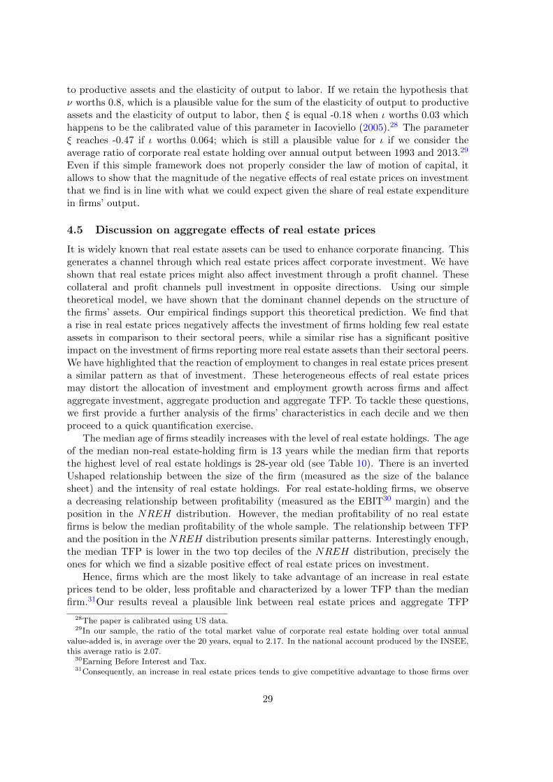
to productive assets and the elasticity of output to labor. If we retain the hypothesis thatν worths 0.8, which is a plausible value for the sum of the elasticity of output to productiveassets and the elasticity of output to labor, then ξ is equal -0.18 when ι worths 0.03 whichhappens to be the calibrated value of this parameter in Iacoviello (2005).28 The parameterξ reaches -0.47 if ι worths 0.064; which is still a plausible value for ι if we consider theaverage ratio of corporate real estate holding over annual output between 1993 and 2013.29

Even if this simple framework does not properly consider the law of motion of capital, itallows to show that the magnitude of the negative effects of real estate prices on investmentthat we find is in line with what we could expect given the share of real estate expenditurein firms’ output.

4.5 Discussion on aggregate effects of real estate prices

It is widely known that real estate assets can be used to enhance corporate financing. Thisgenerates a channel through which real estate prices affect corporate investment. We haveshown that real estate prices might also affect investment through a profit channel. Thesecollateral and profit channels pull investment in opposite directions. Using our simpletheoretical model, we have shown that the dominant channel depends on the structure ofthe firms’ assets. Our empirical findings support this theoretical prediction. We find thata rise in real estate prices negatively affects the investment of firms holding few real estateassets in comparison to their sectoral peers, while a similar rise has a significant positiveimpact on the investment of firms reporting more real estate assets than their sectoral peers.We have highlighted that the reaction of employment to changes in real estate prices presenta similar pattern as that of investment. These heterogeneous effects of real estate pricesmay distort the allocation of investment and employment growth across firms and affectaggregate investment, aggregate production and aggregate TFP. To tackle these questions,we first provide a further analysis of the firms’ characteristics in each decile and we thenproceed to a quick quantification exercise.

The median age of firms steadily increases with the level of real estate holdings. The ageof the median non-real estate-holding firm is 13 years while the median firm that reportsthe highest level of real estate holdings is 28-year old (see Table 10). There is an invertedUshaped relationship between the size of the firm (measured as the size of the balancesheet) and the intensity of real estate holdings. For real estate-holding firms, we observea decreasing relationship between profitability (measured as the EBIT30 margin) and theposition in the NREH distribution. However, the median profitability of no real estatefirms is below the median profitability of the whole sample. The relationship between TFPand the position in the NREH distribution presents similar patterns. Interestingly enough,the median TFP is lower in the two top deciles of the NREH distribution, precisely theones for which we find a sizable positive effect of real estate prices on investment.

Hence, firms which are the most likely to take advantage of an increase in real estateprices tend to be older, less profitable and characterized by a lower TFP than the medianfirm.31Our results reveal a plausible link between real estate prices and aggregate TFP

28The paper is calibrated using US data.29In our sample, the ratio of the total market value of corporate real estate holding over total annual

value-added is, in average over the 20 years, equal to 2.17. In the national account produced by the INSEE,this average ratio is 2.07.

30Earning Before Interest and Tax.31Consequently, an increase in real estate prices tends to give competitive advantage to those firms over

29

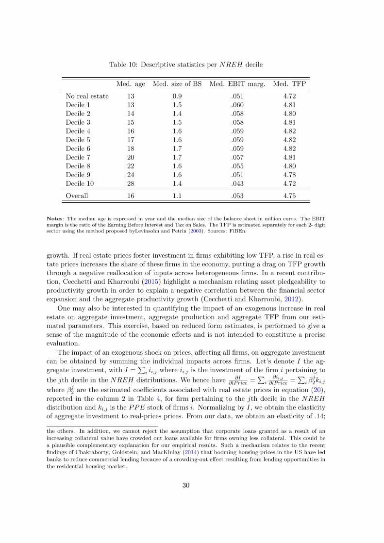
Table 10: Descriptive statistics per NREH decile

Med. age Med. size of BS Med. EBIT marg. Med. TFP

No real estate 13 0.9 .051 4.72Decile 1 13 1.5 .060 4.81Decile 2 14 1.4 .058 4.80Decile 3 15 1.5 .058 4.81Decile 4 16 1.6 .059 4.82Decile 5 17 1.6 .059 4.82Decile 6 18 1.7 .059 4.82Decile 7 20 1.7 .057 4.81Decile 8 22 1.6 .055 4.80Decile 9 24 1.6 .051 4.78Decile 10 28 1.4 .043 4.72

Overall 16 1.1 .053 4.75

Notes: The median age is expressed in year and the median size of the balance sheet in million euros. The EBITmargin is the ratio of the Earning Before Interest and Tax on Sales. The TFP is estimated separately for each 2- digitsector using the method proposed byLevinsohn and Petrin (2003). Sources: FiBEn.

growth. If real estate prices foster investment in firms exhibiting low TFP, a rise in real es-tate prices increases the share of these firms in the economy, putting a drag on TFP growththrough a negative reallocation of inputs across heterogeneous firms. In a recent contribu-tion, Cecchetti and Kharroubi (2015) highlight a mechanism relating asset pledgeability toproductivity growth in order to explain a negative correlation between the financial sectorexpansion and the aggregate productivity growth (Cecchetti and Kharroubi, 2012).

One may also be interested in quantifying the impact of an exogenous increase in realestate on aggregate investment, aggregate production and aggregate TFP from our esti-mated parameters. This exercise, based on reduced form estimates, is performed to give asense of the magnitude of the economic effects and is not intended to constitute a preciseevaluation.

The impact of an exogenous shock on prices, affecting all firms, on aggregate investmentcan be obtained by summing the individual impacts across firms. Let’s denote I the ag-gregate investment, with I =

∑i ii,j where ii,j is the investment of the firm i pertaining to

the jth decile in the NREH distributions. We hence have ∂I∂lPrice =

∑i

∂ii,j∂lPrice =

∑i β

j2ki,j

where βj2 are the estimated coefficients associated with real estate prices in equation (20),reported in the column 2 in Table 4, for firm pertaining to the jth decile in the NREHdistribution and ki,j is the PPE stock of firms i. Normalizing by I, we obtain the elasticityof aggregate investment to real-prices prices. From our data, we obtain an elasticity of .14;

the others. In addition, we cannot reject the assumption that corporate loans granted as a result of anincreasing collateral value have crowded out loans available for firms owning less collateral. This could bea plausible complementary explanation for our empirical results. Such a mechanism relates to the recentfindings of Chakraborty, Goldstein, and MacKinlay (2014) that booming housing prices in the US have ledbanks to reduce commercial lending because of a crowding-out effect resulting from lending opportunities inthe residential housing market.

30

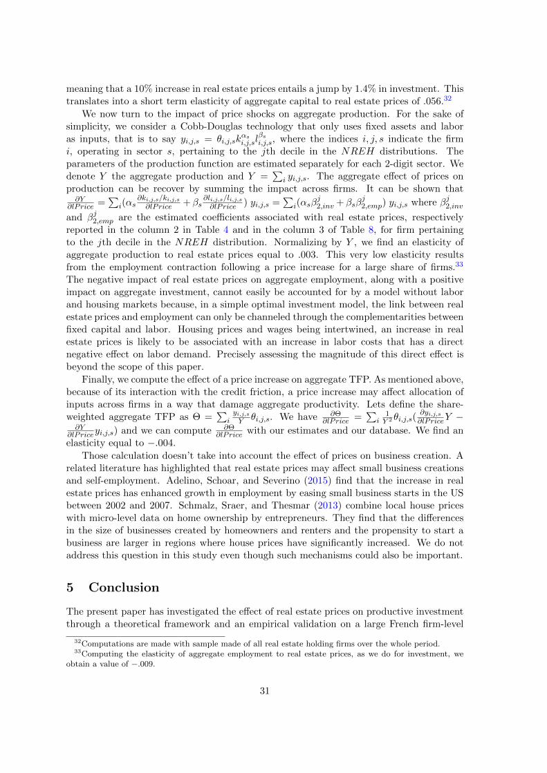
meaning that a 10% increase in real estate prices entails a jump by 1.4% in investment. Thistranslates into a short term elasticity of aggregate capital to real estate prices of .056.32

We now turn to the impact of price shocks on aggregate production. For the sake ofsimplicity, we consider a Cobb-Douglas technology that only uses fixed assets and laboras inputs, that is to say yi,j,s = θi,j,sk

αsi,j,sl

βsi,j,s, where the indices i, j, s indicate the firm

i, operating in sector s, pertaining to the jth decile in the NREH distributions. Theparameters of the production function are estimated separately for each 2-digit sector. Wedenote Y the aggregate production and Y =

∑i yi,j,s. The aggregate effect of prices on

production can be recover by summing the impact across firms. It can be shown that∂Y

∂lPrice =∑

i(αs∂ki,j,s/ki,j,s∂lPrice + βs

∂li,j,s/li,j,s∂lPrice ) yi,j,s =

∑i(αsβ

j2,inv + βsβ

j2,emp) yi,j,s where βj2,inv

and βj2,emp are the estimated coefficients associated with real estate prices, respectivelyreported in the column 2 in Table 4 and in the column 3 of Table 8, for firm pertainingto the jth decile in the NREH distribution. Normalizing by Y , we find an elasticity ofaggregate production to real estate prices equal to .003. This very low elasticity resultsfrom the employment contraction following a price increase for a large share of firms.33

The negative impact of real estate prices on aggregate employment, along with a positiveimpact on aggregate investment, cannot easily be accounted for by a model without laborand housing markets because, in a simple optimal investment model, the link between realestate prices and employment can only be channeled through the complementarities betweenfixed capital and labor. Housing prices and wages being intertwined, an increase in realestate prices is likely to be associated with an increase in labor costs that has a directnegative effect on labor demand. Precisely assessing the magnitude of this direct effect isbeyond the scope of this paper.

Finally, we compute the effect of a price increase on aggregate TFP. As mentioned above,because of its interaction with the credit friction, a price increase may affect allocation ofinputs across firms in a way that damage aggregate productivity. Lets define the share-weighted aggregate TFP as Θ =

∑iyi,j,sY θi,j,s. We have ∂Θ

∂lPrice =∑

i1Y 2 θi,j,s(

∂yi,j,s∂lPriceY −

∂Y∂lPriceyi,j,s) and we can compute ∂Θ

∂lPrice with our estimates and our database. We find anelasticity equal to −.004.

Those calculation doesn’t take into account the effect of prices on business creation. Arelated literature has highlighted that real estate prices may affect small business creationsand self-employment. Adelino, Schoar, and Severino (2015) find that the increase in realestate prices has enhanced growth in employment by easing small business starts in the USbetween 2002 and 2007. Schmalz, Sraer, and Thesmar (2013) combine local house priceswith micro-level data on home ownership by entrepreneurs. They find that the differencesin the size of businesses created by homeowners and renters and the propensity to start abusiness are larger in regions where house prices have significantly increased. We do notaddress this question in this study even though such mechanisms could also be important.

5 Conclusion

The present paper has investigated the effect of real estate prices on productive investmentthrough a theoretical framework and an empirical validation on a large French firm-level

32Computations are made with sample made of all real estate holding firms over the whole period.33Computing the elasticity of aggregate employment to real estate prices, as we do for investment, we

obtain a value of −.009.

31

database.Our theoretical framework models firms’ investment with credit rationing and real estate

assets which can be used as collateral but also as inputs in the production process. Realestate prices operate through two channels with opposite effects on borrowing capacities ofcredit-constrained firms. Through the first channel, an increase in real estate prices raisesthe market value of firms’ pledgeable assets and facilitates their access to credit. Throughthe second channel, this increase raises the cost of structures, decreasing expected profitand damaging borrowing capacities. As a result, the impact of an increase in real estateprices on credit-constrained firms depends on firms’ characteristics, the level of real estateholdings being the main determinant.

Our empirical analysis has validated our main theoretical predictions. The impact ofreal estate prices on productive investment is globally positive, although modest and weaklyrobust. Considering firms’ heterogeneity, we do find a negative impact for firms in the lowerpart of the sectoral distribution of real estate ownership, and a positive impact in the upperpart. These results suggest that French firms have faced binding borrowing constraints overthe studied period.

Hence, real estate price fluctuations affect resources allocation. Real estate price hikestend to favor older and, in average, less productive firms and may have weighed on firms’overall performance and on the creative destruction process in the bubble years. Futureresearch could hence focus on the impact of real estate changes on productivity dynamics,specifically through entry/exit processes.

32

References

[1] M. Adelino, A. Schoar, and F. Severino. “House prices, collateral, and self-employment”.In: Journal of Financial Economics 117.2 (2015), pp. 288–306 (cit. on p. 31).

[2] H. Almeida, M. Campello, and M. Weisbach. “The cash flow sensitivity of cash”. In:The Journal of Finance 59.4 (2004), pp. 1777–1804 (cit. on p. 10).

[3] P. Askenazy. “Capital Prices and Eurozone Competitiveness Differentials”. IZA Dis-cussion Paper, No 7219. 2013 (cit. on p. 1).

[4] T. Beck, A. Demirguc-Kunt, and M.S. Martinez Peria. “Bank financing for SMEsaround the world: Drivers, obstacles, business models, and lending practices”. WorldBank Policy Research Working Paper Series. 2008 (cit. on p. 1).

[5] A. Berger and G. Udell. “Collateral, loan quality and bank risk”. In: Journal ofMonetary Economics 25.1 (1990), pp. 21–42 (cit. on p. 1).

[6] K. Case, J. Quigley, and R. Shiller. “Comparing wealth effects: the stock marketversus the housing market”. In: Advances in macroeconomics 5.1 (2005) (cit. on p. 2).

[7] S. Cecchetti and E. Kharroubi. “Reassessing the impact of finance on growth”. BISWorking Paper. 2012 (cit. on p. 30).

[8] S. Cecchetti and E. Kharroubi. “Why does financial sector growth crowd out realeconomic growth?” BIS Working Paper. 2015 (cit. on p. 30).

[9] G. Cette, S. Corde, and R. Lecat. “”Rupture de tendance de la productivite en France: quel impact de la crise ?””. mimeo. 2017 (cit. on p. 2).

[10] G. Cette, J. Fernald, and B. Mojon. “The pre-Great Recession slowdown in produc-tivity”. In: European Economic Review 88 (2016), pp. 3–20 (cit. on p. 1).

[11] I. Chakraborty, I. Goldstein, and A. MacKinlay. “Do asset price bubbles have negativereal effects?” Mimeo, Wharton School, University of Pennsylvania. 2014 (cit. on p. 30).

[12] T. Chaney, D. Sraer, and D. Thesmar. “The Collateral Channel: How Real EstateShocks Affect Corporate Investment”. HEC Working Paper. 2009 (cit. on p. 3).

33

[13] T. Chaney, D. Sraer, and D. Thesmar. “The Collateral Channel: How Real EstateShocks Affect Corporate Investment”. In: The American Economic Review 102 (2012),pp. 2381–2409 (cit. on p. 1).

[14] T. Chaney, D. Sraer, and D. Thesmar. “Real Estate Collateral and Labor Demand”.Mimeo, Toulouse School of Economics. 2013 (cit. on pp. 2, 11, 12).

[15] P.P. Combes and L. Gobillon. “The empirics of agglomeration economies”. Mimeo,Sciences Po. 2014 (cit. on p. 4).

[16] G. Favara and J. Imbs. “Credit supply and the price of housing”. In: The AmericanEconomic Review 105.3 (2015), pp. 958–992 (cit. on p. 2).

[17] D. Fougere and M. Poulhes. “The Effect of Housing on Portfolio Choice: A ReappraisalUsing French Data”. In: CEPR Discussion Paper No. 9213 (2012) (cit. on pp. 9, 38).

[18] J. Friggit. “Le prix des logements sur longue periode”. In: Informations sociales 155.5(2009), pp. 26–33 (cit. on pp. 9, 38).

[19] J. Gan. “Collateral, debt capacity, and corporate investment: Evidence from a naturalexperiment”. In: Journal of Financial Economics 85.3 (2007), pp. 709–734 (cit. onp. 1).

[20] O. Hart and J. Moore. “Property Rights and the Nature of the Firm”. In: Journal ofpolitical economy (1990), pp. 1119–1158 (cit. on p. 2).

[21] M. Iacoviello. “House Prices, Borrowing Constraints, and Monetary Policy in theBusiness Cycle”. In: American Economic Review 95.3 (2005), pp. 739–764 (cit. onp. 29).

[22] L. Kaas, P. Pintus, and S. Ray. “Land collateral and labor market dynamics inFrance”. In: European Economic Review (2014) (cit. on p. 1).

[23] S. Kaplan and L. Zingales. “Do investment-cash flow sensitivities provide useful mea-sures of financing constraints?” In: The Quarterly Journal of Economics (1997),pp. 169–215 (cit. on p. 10).

[24] N. Kiyotaki and J. Moore. “Credit Cycles”. In: Journal of Political Economy 105(1997), pp. 211–248 (cit. on p. 1).

34

[25] J. Levinsohn and A. Petrin. “Estimating production functions using inputs to controlfor unobservables”. In: The Review of Economic Studies 70.2 (2003), pp. 317–341(cit. on pp. 10, 11, 15, 30).

[26] Z. Liu, P. Wang, and T. Zha. “Land-Price Dynamics and Macroeconomic Fluctua-tions”. In: Econometrica 81.3 (2013), pp. 1147–1184 (cit. on p. 1).

[27] N. Mora. “The effect of bank credit on asset prices: evidence from the Japanese realestate boom during the 1980s”. In: Journal of Money, Credit and Banking 40.1 (2008),pp. 57–87 (cit. on p. 2).

[28] M. Schmalz, D. Sraer, and D. Thesmar. “Housing collateral and entrepreneurship”.National Bureau of Economic Research No. 19680. 2013 (cit. on p. 31).

[29] J. Tirole. The theory of corporate finance. Princeton University Press, 2010 (cit. onpp. 2–4).

[30] J. Wu, J. Gyourko, and Y. Deng. “Real estate collateral value and investment: Thecase of China”. In: Journal of Urban Economics 86 (2015), pp. 43–53 (cit. on p. 2).

35

6 Appendix

6.1 Appendix A: Proof of proposition 1

We know that i∗and R∗ maximize the objective function. Let’s the function V (i, R) denotethe value of the objective function associated with an investment i and a number of realestate units R. By definition, ∀(g, h) ∈ R2, V (i∗+g,R∗+h)−V (i∗, R∗) ≤ 0. A second-orderTaylor approximation of the function V around (i∗, R∗) gives:

V (i∗ + g,R∗ + h)− V (i∗, R∗) ≈ ykk(k∗, R∗, θ)

1 + rg2

+2ykR(k∗, R∗, θ)

1 + rgh+

yRR(k∗, R∗, θ)

1 +Rh2

(22)

Dividing by h2 we have:

V (i∗ + g,R∗ + h)− V (i∗, R∗)

h2≈ ykk(k

∗, R∗, θ)

1 + r

g2

h2

+2ykR(k∗, R∗, θ)

1 + r

g

h+yRR(k∗, R∗, θ)

1 +R

(23)

We know that, ∀g ∈ R, ∀h ∈ R∗:

V (i∗ + g,R∗ + h)− V (i∗, R∗)

h2< 0 (24)

Hence we can write:(2ykR(k∗, R∗, θ)

1 + r

)2

− 4ykk(k

∗, R∗, θ)

1 + r

yRR(k∗, R∗, θ)

1 + r< 0 (25)

and eventually:

ykR(k∗, R∗, θ)2

yRR(k∗, R∗, θ)− ykk(k∗, R∗, θ) > 0 (26)

6.2 Appendix B: Proof of proposition 2

Let F be a function of i, with i ∈ [0, i∗] such that:

F (i) = (1 + r) +L− S + pR0

L(y(k0 + i, R, θ)− rp(R−R0))− (1 + r)i− (1 + r)B0 (27)

We get:

∂F

∂i(i) =

L− S + pR0

Lyk(k0 + i, R, θ)− (1 + r) (28)

And:

∂2F

∂i∂i(i) =

L− S + pR0

Lykk(k0 + i, R, θ) (29)

36

From the properties of the function y we deduce that; ∀i ∈ [0, i∗], ∂2F (i)∂i∂i < 0. We know

that, in the constrained case, L−S+pR0

L ∈ [0, 1]. From the first equation in system (6), we

know that ∂F∂i (i∗) < 0.

We distinguish two cases:

• If ∂F∂i (0) < 0, we conclude that, ∀i ∈ [0, i∗]:

(1 + r)− L− S + pR0

Lyk(k0 + i, R, θ) > 0 (30)

• If ∂F∂i (0) ≥ 0, we know that there exists a unique threshold i ∈ [0, i∗) such that

∂F∂i (i) < 0 if and only if i > i. The function F is increasing on the interval [0, i] anddecreasing on the interval [i, i∗]. The constraint on the initial amount of debt, i.e.,L−S+pR0

L (y(k0, R, θ)− cre(R)) ≥ (1+r)B0, insures that F (0) > 0 and we deduce fromthe variation of F that the value i satisfying F (i) = 0 pertains to the interval (i, i∗].Thus, when i denotes the investment in the constrained case, we also have:

(1 + r)− L− S + pR0

Lyk(k0 + i, R, θ) > 0 (31)

We conclude that the sign of ∂i∂p is determined by the sign of P (R0).

The discriminant of the polynomial P is strictly positive and P (0) < 0. We know thatP has a unique positive real root R and we conclude that ∂i

∂p ≥ 0 if and only if R0 ≥ R,with:

R =2prR− y(k,R, θ)− r(L− S) +

√[y(k,R, θ)− 2rpR+ r(L− S)]2 + 8r2p(L− S)R

4rp(32)

Note that the relative position of R to Sp depends on the parameters value and the

functional form of y.The sign of ∂i

∂R0, ∂i∂c0

, ∂i∂B0

and ∂i∂θ can be obtained thanks to the result derived above.

We have:

∂i

∂R0=

L−S+pR0

L rp+ pL [y(k,R, θ)− rp(R−R0)]

(1 + r)− L−S+pR0

L yk(k,R, θ)> 0 (33)

∂i

∂c0=

1

(1 + r)− L−S+pR0

L yk(k,R, θ)> 0 (34)

∂i

∂B0=

−1

(1 + r)− L−S+pR0

L yk(k,R, θ)< 0 (35)

∂i

∂θ=

L−S+pR0

L yθ(k,R, θ)

(1 + r)− L−S+pR0

L yk(k,R, θ)> 0 (36)

6.3 Appendix C: Further details on real estate price indices

6.4 Appendix D: Further details on real estate partnerships

37

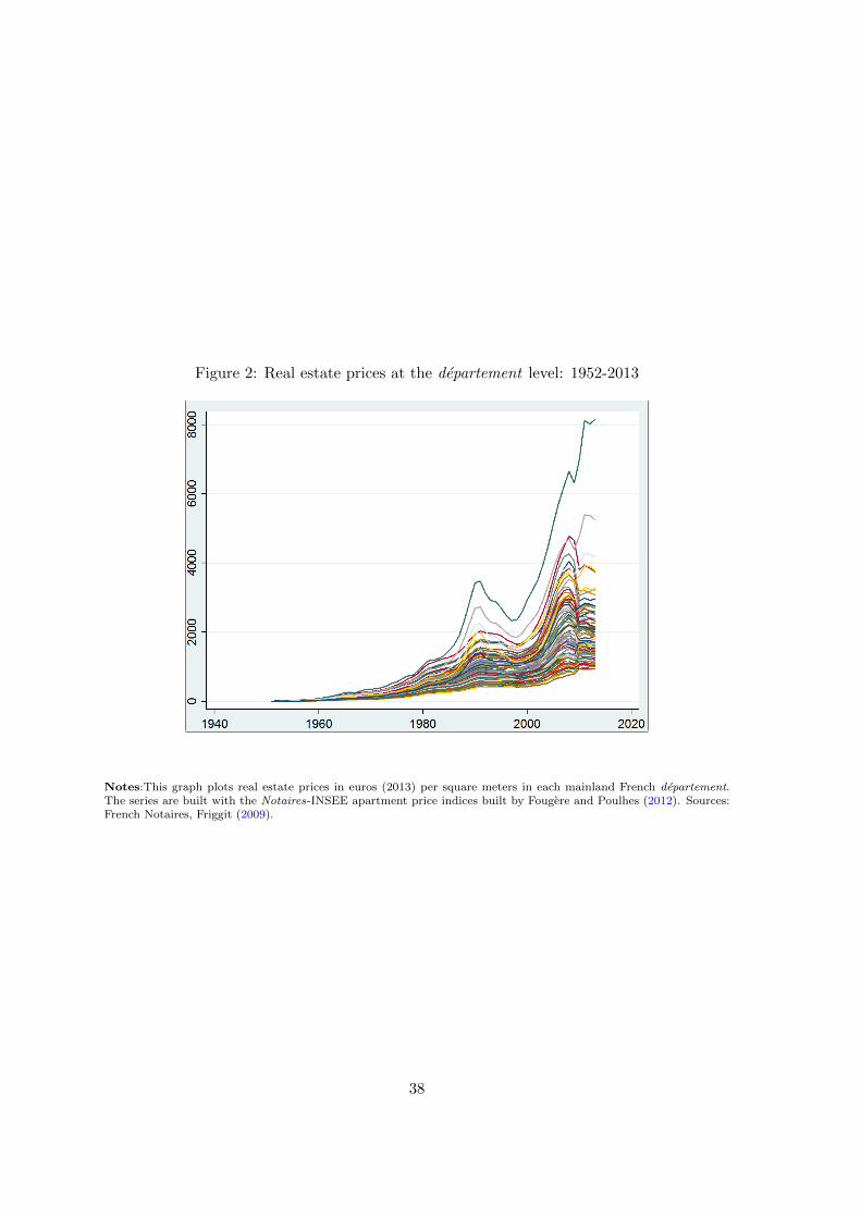
Figure 2: Real estate prices at the departement level: 1952-2013

Notes:This graph plots real estate prices in euros (2013) per square meters in each mainland French departement.The series are built with the Notaires-INSEE apartment price indices built by Fougere and Poulhes (2012). Sources:French Notaires, Friggit (2009).

38

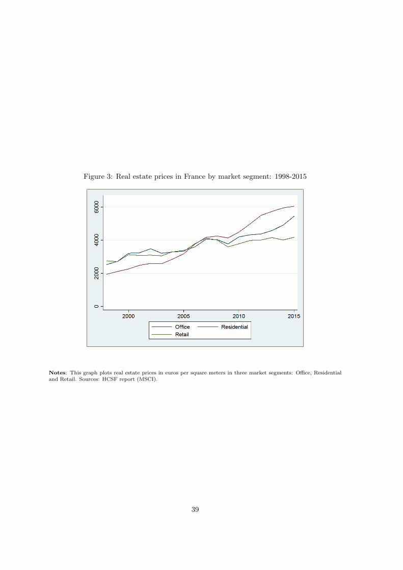
Figure 3: Real estate prices in France by market segment: 1998-2015

Notes: This graph plots real estate prices in euros per square meters in three market segments: Office, Residentialand Retail. Sources: HCSF report (MSCI).

39

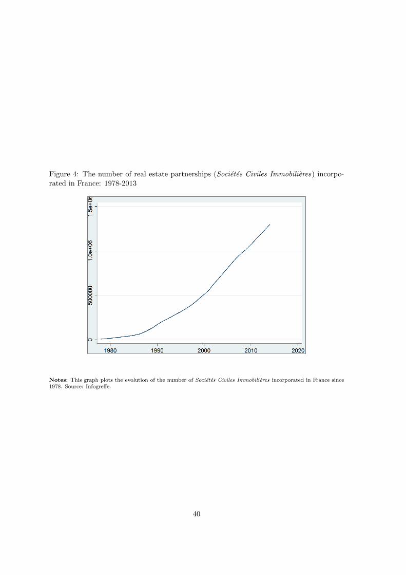
Figure 4: The number of real estate partnerships (Societes Civiles Immobilieres) incorpo-rated in France: 1978-2013

Notes: This graph plots the evolution of the number of Societes Civiles Immobilieres incorporated in France since1978. Source: Infogreffe.

40