Real-Business-Cycle Models and the Forecastable …people.hbs.edu/jrotemberg/PublishedArticles/Real... · Real-Business-Cycle Models and the ... model cannot account for the observed

Real-Business-Cycle Models and the Forecastable Movements in Output, Hours,and Consumption

Julio J. Rotemberg; Michael Woodford

The American Economic Review, Vol. 86, No. 1. (Mar., 1996), pp. 71-89.

Stable URL:

http://links.jstor.org/sici?sici=0002-8282%28199603%2986%3A1%3C71%3ARMATFM%3E2.0.CO%3B2-Y

The American Economic Review is currently published by American Economic Association.

Your use of the JSTOR archive indicates your acceptance of JSTOR's Terms and Conditions of Use, available athttp://www.jstor.org/about/terms.html. JSTOR's Terms and Conditions of Use provides, in part, that unless you have obtainedprior permission, you may not download an entire issue of a journal or multiple copies of articles, and you may use content inthe JSTOR archive only for your personal, non-commercial use.

Please contact the publisher regarding any further use of this work. Publisher contact information may be obtained athttp://www.jstor.org/journals/aea.html.

Each copy of any part of a JSTOR transmission must contain the same copyright notice that appears on the screen or printedpage of such transmission.

The JSTOR Archive is a trusted digital repository providing for long-term preservation and access to leading academicjournals and scholarly literature from around the world. The Archive is supported by libraries, scholarly societies, publishers,and foundations. It is an initiative of JSTOR, a not-for-profit organization with a mission to help the scholarly community takeadvantage of advances in technology. For more information regarding JSTOR, please contact [email protected].

http://www.jstor.orgWed Nov 28 14:03:11 2007


http://www.jstor.org/about/terms.html

http://www.jstor.org/journals/aea.html

Real-Business-Cycle Models and the Forecastable Movements in Output, Hours, and Consumption

We study the movements in output, consumption and hours that are forecastable from a VAR and analyze how they differ from those predicted by standard real- business-cycle models. We show that actual forecastable movements in output have a variance about one hundred times larger than those predicted by the model. We also jnd that forecastable changes in the three series are strongly positively correlated with each other. On the other hand, for parameters whose implications are plausible in other respects, the model implies that output, consumption, and hours should not all be expected to move in the same direction. (JEL E32, E37)

In this paper we analyze the degree to which standard real-business-cycle (RBC) models are consistent with the forecastable move-ments in output, consumption, and hours. We focus on forecastable movements in our variables because it is arguable that these consti- tute the essence of what it means for these variables to be "cyclical." In particular, Stephen Beveridge and Charles R. Nelson ( 198 1 ) define the cyclical component of a series X , as

(1) X;Yc= lim E,[X, - X, + ,+ T log y,] T-rW

where yx is the unconditional expectation of the rate of growth of X. In other words, the cyclical component of X is the difference between its current value and the value it is expected to have in the indefinite future, as long as one abstracts from the unconditional mean of the growth of X. Ignoring this mean growth, the cyclical value is thus nothing more than

* Rotemberg: Sloan School of Management, Massa- chusetts Institute of Technology, 50 Memorial Drive, Cambridge, MA 02142-1347; and Woodford: Depart- ment of Economics, Princeton University, Princeton, NJ 08544. We wish to thank Ludwig Chincarini for research assistance, John Cochrane, John Huizinga, Lucrezia Reichlin, and Argia Sbordone for helpful discussions, two referees and Ken West for comments, and the National Science Foundation for research support.

the amount by which the series can be expected to decline.

One of the principal attractions of the RBC model is its parsimony. The model is supposed to explain growth that is simultaneous with the business cycle using only one set of shocks, namely stochastic variations in the rate of technical progress (Finn E. Kydland and Edward C. Prescott, 1982; Prescott, 1986; Robert G. I(mg et al., 1988a, 1988b; Charles I. Plosser, 1989). For this model to explain growth (as opposed to having growth come from a different source), these stochastic variations in technology must be permanent. This leads us to follow the literature that assumes that technology follows a random walk and that, as a result, output contains a unit root.'

We then show that, although the model is constructed so that it can explain the stochastic trend in output, it is unable to account for the business cycle as we define it. In particular, it is unable to account for many features of the forecastable movements in output,

' The existence of a unit root in output remains contro- versial (e.g., Glenn D. Rudebusch, 1993). We take this view here because it is frequently argued that such a unit root exists, and that this is in itself important evidence in favor of RBC models (Nelson and Plosser, 1982; King et al., 1991). We also find it desirable to model "trend" growth in output as not being constant over our sample period, while still requiring our theoretical model to si- multaneously account for both the "trend" and "cyclical" components of output.

i' I

72 THE AMERICAN ECONOMIC REVIEW MARCH 1996

consumption, and hours. In the model, a shock that improves technological opportunities leads to a period of capital accumulation, and this generates forecastable movements in output, consumption, and hours. However, we show that these forecastable movements generated by the model are small both in absolute terms (given the size of changes in productivity) and relative to the overall size of the movements in output. In particular, we show that the variance of predictable output movements implied by the model equals about 1 percent of the actual variance of forecastable movements in output over the next 12 months. This point is closely related to criticisms of the RBC model by Mark W. Watson (1993) and Timothy Cogley and James M. Nason (1995). The latter, in particular, show that variants of the RBC model cannot account for the observed degree of serial correlation of output growth.'

Furthermore, the forecastable movements generated by the model are of the wrong kind. The data suggest that forecastable movements in output, consumption, and hours are strongly, positively correlated. By contrast the standard RBC model requires that some of these correlations be negative. As we show below, a technology shock that raises output also implies that the inherited capital stock is below the steadv-state value of the capital stock. This leads real interest rates to rise and, as a result, the current level of consumption must also be below the steady-state level of consumption. Thus this shock leads to forecastable increases in consumption. On the other hand, a standard parametrization of preferences implies that technology shocks that raise output also raise the current level of

'This serial correlation is the source of some, though not all, of the predictable movements in output that we document, for the forecastable component of output movements is found to be significantly larger when a multivariate-forecasting model is used (John H. Cochrane and Argia Sbordone, 1988; George W. Evans and Lucrezia Reichlin, 1994). Our test is also not equivalent to the "impulse response function" test of Cogley and Nason (1995). Unlike that test, our measurement of the size of the forecastable movements in output identifies a statistic about which standard single-shock RBC models make a prediction.

hours. Since hours are stationary in the model, this means that hours are forecasted to decline. The model thus typically implies that hours and consumption are expected to move in opposite directions."

Using standard parameters, a positive technology shock raises contemporaneous output by less than it raises the expected steady-state level of output. It thus leads to forecastable increases in output and, as a result, the model implies that forecastable increases in output are positively correlated with forecastable increases in consumption and negatively correlated with forecastable increases in hours. The use of alternative parameters, and in particular the use of a high elasticity of labor supply and a high labor share, can change this result. In particular, it can cause the immediate increase in output due to a positive technology shock to be larger than the long-run increase. Such a shock thus leads to expected-output declines, which means that expected-output movements should be positively correlated with expected- hours movements, but negatively correlated with expected-consumption movements.

In Section I, we document the forecastable changes in output and other aggregate quantities for the postwar United States, using a simple vector-autoregression (VAR) frame- work. In addition to showing the importance of these forecastable changes, we show that a definition of the business cycle in terms of variations in forecasted private-output growth coincides empirically with other familiar def-

'This failure of the model thus appears related to the failures of the representative agent model of labor supply documented by N. Gregory Mankiw et al. (1985). They argue that the procyclical movements of observed real wages are too slight for a rational household with well behaved preferences to choose movements in consumption and hours that are as positively correlated as those found in U.S. data. The current study differs in two ways. First, we focus only on predictable movements whereas Mankiw et al. look at overall movements. This makes a big difference because the RBC model with standard parameter values does predict that unexpected movements in hours and consumption should be positively correlated. Second, we follow the RBC literature in neglecting real- wage observations so that, in principle, the model could be generating real wages that make households choose forecastable movements in consumption and labor supply that are positively correlated.

73 VOL. 86 NO. I ROTEMBERG AND WOODFORD: RBC AND FORECASTABLES

initions; for example, we show that our dat- ing of cycles on these grounds would be similar to that of the National Bureau of Eco- nomic Research (NBER). In Section 11, we review the predictions of a simple RBC model regarding forecastable changes in aggregate quantities. In Section 111, we present the numerical predictions from a calibrated version of the model that uses standard parameter values and compare them to our empirical results. Section IV considers the effect of varying the preference parameters of the model. Section V concludes.

I. Forecastable Movements in Output, Consumption and Hours

In this section we describe the statistical properties of aggregate U.S. output, con-sumption, and hours. In particular, we use a three-variable VAR that includes these variables to study the existence of a "business cycle" in the sense of forecastable changes in these variables. We use these three variables because we wish to compare the properties of the U.S. data to the predictions of a standard stochastic-growth model. This requires that we use series that represent empirical correlates of variables that are determined in that model. The RBC literature has stressed its predictions for the movements in aggregate output, consumption, and hours. Moreover, the estimation of a joint stochastic process for these three variables also implies processes for labor productivity (output per hour) and investment (output that is not consumed). Thus, we are in fact estimating the joint behavior of all the main variables for which the model makes predictions.

The simple "permanent-income hypothe-sis" provides an additional reason for including consumption in our VAR since the theory implies that the share of consumption in total output should forecast future output growth. This prediction has been verified by John Y. Campbell (1987), Cochrane and Sbordone (1988), Cochrane (1994a), and King et al. ( 1991) . Likewise, the idea that variations in the labor input can be used to predict future changes in output has been used to identify temporary output fluctuations in a VAR frame- work by Olivier J. Blanchard and Danny Quah

( 1989) and Evans ( 1989) .4 Furthermore, as we explain in the next section, the stochastic-growth model implies that expected growth is a function of a certain state variable (the aggregate capital stock relative to the technology-adjusted labor force). According to that model, both the consumption-output ratio and hours relative to the labor force should also be functions of that state variable, and hence either variable should supply all of the information that is relevant for forecasting future output growth.

As we explain in the next section, we inter- pret this standard model as applying to fluctuations in private output and hours. As a consequence, our output measure is real private value-added ~ u t p u t , ~ and our hours measure is hours worked in the private ~ e c t o r . ~ Because we assume that technology shocks lead to permanent changes in technological opportunities, we suppose that the change (but not the level) of private value-added output is stationary. Hours are subject to long-term changes as well if the labor force grows. In this paper, we assume that the long-term growth of the labor force can be modeled as a deterministic trend. The model we develop below then implies that hours are trend stationary. This is not inconsistent with the data; the last column of Table 1 reports a rejection, using a Dickey-Fuller test, of the hypothesis that private hours have a unit root once one allows for a deterministic trend.7

These authors use the unemployment rate, rather than hours, as their measure of variations in the labor input. For our purposes, hours are preferable, because of their clearer relation to the labor input with which the RBC model is concerned. Because detrended private hours are stationary, as discussed below, they can serve as a cyclical indicator in a way similar to the unemployment rate.

We measure real private value-added output, or "private output," as the difference between real GDP and government sector value-added output, both measured in 1987 dollars. Using CITIBASE mnemonics, it equals GDPQ -GGNPQ.

'Our measure of private hours comes from the U.S. Department of Commerce's Survey of Current Business. It equals the private sector employee hours for wage and salary workers in nonagricultural establishments. We are thus implicitly assuming that changes in agricultural hours are proportional to changes in private nonagricultural hours. 'Our results are similar when (like Cogley and Nason,

1995) we use per capita hours rather than detrended hours.

74 THE AMERICAN ECONOMIC REVIEW MARCH I996

Because the consumption decision modeled in the standard growth model is a demand for a nondurable consumption good, we use con- sumer expenditure on nondurables and ser-vices as our measure of consumption. This is also the consumption measure that one has the most reason to expect to forecast future output on permanent-income grounds, and it is the one used in the studies of output forecastabil- ity mentioned above.'

The time series that we use, then, are the logarithms of private output, consumption of nondurables and services, and detrended private hours. Letting lower case letters denote the logarithm of the respective upper case letters, these variables are y,, c, and h,, respe~tively.~

As King et al. (1988b) emphasize, a standard growth model with a random walk in technology implies that y, and c, should be difference-stationary while c, - y, is predicted to be stationary. Table 1 shows that, just as in King et al. ( 1991) ,our data are consistent with these predictions. Hence our VAR specification is

We prefer to emphasize the results using detrended hours because per capita hours still have a slight deterministic trend; that is, if one allows for a trend in an autoregression of per capita hours, one can reject the hypothesis of a zero coefficient on the trend (even though the series passes some tests of stationarity, and the estimated trend growth rate is small).

For our measure of consumption to be strictly com- parable to our measure of output, it should include only consumption of privately provided goods and services. Unfortunately, our measure of consumption does include some government value-added output, particularly value added by state enterprises like the Tennessee Valley Au- thority. In all likelihood, this creates only a small mis- match between our consumption and output measures.

We use these three series to derive the behavior of investment and productivity in a way that is consistent with our theoretical model's accounting identities. Thus we construct a series for the growth rate of investment using the relation

scAc, + (1 - s,)Ai, = Ay,.

Following the calibration of Gary D. Hansen and Randall Wright (1992), we set s, equal to 0.74.We similarly construct our series for growth in labor productivity from our series for growth of output and hours, using the relation

Apt = Ay, - Ah,.

where

U , = and E, =

and only the first three rows of A need to be estimated. We denote the variance-covariance matrix of E, by 52,. This autoregression includes only two lags. One reason for ignoring further lags is that, when we included them, these were generally not statistically significantly different from 0. A second reason is that we want to avoid overfitting our VAR. Overfitting is a particular concern in that it could lead us to overstate the extent to which aggregate variables are forecast-able, and thus the extent to which they are subject to cyclical movements. Table 1 also presents the estimates from our VAR. As can be seen from the table, most parameters are statistically different from zero.

We now discuss how the VAR can be used to obtain statistics relating to expected movements in our variables. We let Ay: den2te the hfference between y, +, and y, while Ayf de-notes the expectation at time t of this difference. It is given by

(3) Kyf= Bt u,,

where e , is a vector that has a one in the first position and zeros in all others. For the case where k = m , we have (minus) the Beveridge-Nelson ( 198 1 ) definition of the cyclical component of log Y,, which is given by

The expecgd percentage change in con-sumption, Ac: is similarly given by

VOL. 86 NO. 1 ROTEMBERG AND WOODFORD: RBC AND FORECASTABLES 75

Explanatory variables AY (C - Y) h Ay' A(c - Y) Ah

Constant

AY-I

AY-2

(c - Y)-1

(c - Y)-2

h-1

h-2

Ay!,

Ay Z2

A(c - Y)-1

A(c - Y)-2

Ah-,

Ah-2

Trend

Notes: Data are from 1948.4 to 1993.2. Standard errors are given in parentheses below coefficient estimates. Ay denotes the change in the log of private value added, c - y denotes the log of the ratio of consumption to output and h denotes the log of private man hours in nonagricultural establishments (these are detrended in the first three columns).

= Btu, where e2 is a vector whose second element equals one while the others equal zero and the second equality defines B:. The expected percentage change in hours is given by

(5) f h f = e S A k u , - h , = B t u ,

where e, is defined analogously to el and e2 while the second equality defines Bk,. The expected percentage changes in investment and in productivity are then computed as linear combinations of these.

Letting 'U denote the vari'nce-cova'ance

Standard deviations for both actual- and expected-output changes over different horizons are presented in Table 2. This table also presents a measure of uncertainty for the standard deviations of expected-output changes. This measure of uncertainty is the standard error of the estimate based on the uncertainty concerning the elements of A and those of S2,.10

l o Uncertainty about both of these elements leads to uncertainty about the quantity in (6) because B{ de-pends on A while 0, (which equals A0,A' + n,) de-pends on both A and n , . Note that vec(S2,) is equal to (1- A ) - I ~ ~ ~ ( ~ , ) ,A using this formula, we can corn-

matrix of ur,/\our estimate of the ( ~ o ~ u l a t i o n ) pute the formula in (6) for different values of the ele- variance of Ayk is ments of A and 0, . We thus obtain the vector of


Horizon (in quarters) 1 2 4 8 12 24 to

Standard deviation of:

xotes: Asymptotic standard errors are in parentheses. Ay: denotes the change in the log of output from t to t + k while Ay: denotes the expectation of this change based on information available at t.

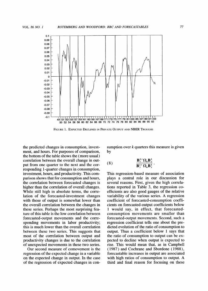
The table shows that the standard deviation of the expected changes for output grows as the horizon lengthens from 1 to 12 quarters. Because the predictable movements in output are largest at the 12-quarter horizon, we focus mostly on this horizon. The standard deviation of the predictable movements over this horizon is above 3.2 percent. To assess the importance of these movements, it is worth looking at the last row of the table which gives the standard deviation of total output movements. This comparison shows that the variance of the predictable movements in output equals over half of the variance of total movements in output over this horizon.

Figure 1 displays the demeaned expected declines in output over this horizon." We show expected declines, as opposed to ex-pected increases, because recessions ought to be associated with expected increases in output and we wish to represent these as low values for our cyclical indicator. In this figure we

numerical derivatives D of our estimate of the standard deviation of A 9 with respect to both the elements of A and those of O,. The variance of our estimate is then D'OD where O is the variance-covariance matrix of a vector that contains both the elements of A and those of O,, as in James D. Hamilton (1994 p. 301). Note that, the overlapping nature of the data 2ne would have to use to construct sample values of A$ does not affect our calculations because we do not use such sample values to compute the standard deviation of Ayk.

" It is important to note, however, that the expected movements in output over the next 8, 12 or infinite quarters are very similar to each other. Similarly, Rotemberg (1994) shows that the expected movements in output are nearly the same when the VAR also includes inflation and interest rates among its variables.

have also indicated the troughs of recessions as determined by the NBER. We see that output is expected to grow fast at these NBER troughs, so that our measure of the business cycle coincides closely with the NBER's dat- ing of the business cycle.I2

In Tables 3 and 4 we analyze the comovements between the expected changes in our five series. We consider two measures of these comovements. The first is the correlation between the forecasted movements in two series for a given horizon. We illustrate how we compute this correlation by focusing on the correlation of consumption and output changes that are expected to occur over the next k quarters. Our estimate of the (popula- tion) covariance of these series is given by B,k1C4,B$.Thus, the correlation between these two series is given by

Other correlation coefficients are computed analogously. Table 3 shows that the predicted changes in output are highly correlated with

l 2 The one case where the indicators differ is in the case of the last recession. As would be suggested by our series, the recovery from this "trough" was initially weak. It is also worth noting that our series for expected declines in output is quite similar to the series for linearly detrended output. This means that our assumption that output has a unit root probably has a relatively small effect on our results.


FIGURE1. EXPECTEDDECLINES OUTPUTIN PRIVATE AND NBER TROUGHS

the predicted changes in consumption, investment, and hours. For purposes of comparison, the bottom of the table shows the (more usual) correlation between the overall change in output from one quarter to the next and the corresponding 1-quarter changes in consumption, investment, hours, and productivity. This comparison shows that for consumption and hours, the correlation between forecasted changes is higher than the correlation of overall changes. While still high in absolute terms, the correlation of the forecasted-investment changes with those of output is somewhat lower than the overall correlation between the changes in these series. Perhaps the most surprising fea- ture of this table is the low correlation between forecasted-output movements and the corresponding movements in labor productivity; this is much lower than the overall correlation between these two series. This suggests that most of the correlation between output and productivity changes is due to the correlation of unexpected movements in these two series.

Our second measure of comovement is the regression of the expected change in a variable on the expected change in output. In the case of the regression of expected changes in con-

sumption over k quarters this measure is given by

This regression-based measure of association plays a central role in our discussion for several reasons. First, given the high correlations reported in Table 3, the regression coefficients are also good gauges of the relative variability of the various series. A regression coefficient of forecasted-consumption coefficients on forecasted-output coefficients below 1 would say, in effect, that forecasted-consumption movements are smaller than forecasted-output movements. Second, such a regression coefficient tells one about the predicted evolution of the ratio of consumption to output. Thus a coefficient below 1 says that the ratio of consumption to output can be expected to decline when output is expected to rise. This would mean that, as in Campbell (1987) and Cochrane and Sbordone ( 1988), forecastable increases in output are associated with high ratios of consumption to output. A third and final reason for focusing on these


Horizon (in quarters) corr(n^cC:, n̂ y Y : )

1 0.693 (0.121)

2 0.777 (0.083)

4 0.818 (0.071)

8 0.819 (0.068)

12 0.787 (0.070)

24 0.716 (0.092)

w 0.682 (0.127)

corr(n^ii:, n̂ y:)

0.977 (0.010) 0.976

(0.011) 0.976

(0.011) 0.971

(0.014) 0.955

(0.023) 0.886

(0.061) 0.815

(0.143)

corr(&h h: , n̂ yY : ) corr(LpY:, n̂ y Y:)

0.876 -0.153 (0.044) (0.170) 0.887 -0.130

(0.042) (0.190) 0.915 0.043

(0.028) (0.242) 0.965 0.036

(0.012) (0.382) 0.977 -0.081

(0.008) (0.469) 0.978 -0.093

(0.009) (0.494) 0.978 -0.092

(0.010) (0.553)

A

Notes: Asymptotic standard errors are in parentheses, Az,denotes the change in z from t to t + 1 while Az: denotes the conditional expectation of the change from t to t + k based on information available at t. Correlations among expected changes are computed as in (7).

regression-based measures is that, insofar as predictable output movements are a good measure of the busihess cycle, they provide an eco- nomical way of discussing the way in which other variables move over the cycle. In particular, they indicate the percentage by which a given variable can be expected to change if one knows that output is expected to increase by 1 percent.

Table 4 presents regression coefficients of the expected changes in c , i , h and p on expected changes in y . The table shows that, as in our discussion above, the elasticity of expected-consumption growth with respect to expected-output growth is less than 1; it is actually below 0.6 for the infinite horizon and is even lower for shorter horizons."

''Note that the intertemporal budget constraint does not imply that this elasticity ought to be 1 at the infinite horizon. Indeed, the simple permanent income hypothesis implies that the coefficient ought to be 0 because consumption changes should be unpredictable. Our finding that the coefficient is positive is consistent with the large number of studies which have found "excess sensitivity" of consumption to income changes.

Whlle the elasticity of expected-consumption growth with respect to output growth is low, the corresponding elasticity of investment growth is substantial. This means that expected-investment changes are very volatile. Expected-hours growth responds nearly one for one to expected changes in output. This means not only that the series for expected growth in hours is about as volatile as the series for expected-output growth but also that expected-output changes are not associated with significant expected changes in productivity.

II. A Simple Stochastic Growth Model

In this section we discuss some properties of a stochastic-growth model of the lund that is standard in the RBC literature. The purpose of this discussion is to provide intuition for the sort of predictable movements in aggregate variables that the model generates. We show that, when technological opportunities follow a random walk so that the model does indeed generate stochastic growth, all the predictable movements implied by the model are those as-

79 VOL. 86 NO. 1 ROTEMBERG AND WOODFORD: RBC AND FORECASTABLES

Horizon (in quarters) &:on &: Kii: on &: on &: Kp:on Kyi:

Notes: Asymptotic standard errors are in parentheses. &: denotes the expectation conditional on information held at t of the change in z from t to t + k. Regression coefficients are computed as in (8).

sociated with the adjustment of the capital stock towards its steady-state level. In other words, there is a single-state variable, namely the ratio of the current capital stock to its steady-state level, which explains all the predictable movements generated by the model.

The question of -whether the model is capable of reproducing the predictable movements we observe then boils down to two issues. The first is whether changes in capital accumulation attributable to technology shocks can generate predictable output movements of sufficient magnitude. The second is whether the adjustment of capital to its steady state implies, for plausible parameter values, that output, consumption, hours, and investment all move in the same direction.

Our model is essentially identical to the model analyzed in King et al. (1988b) and Plosser (1989) and differs from other real- business-cycle models such as Prescott ( 1986) and Hansen and Wright ( 1992) only in that it assumes a random walk in technology. In or- der to tighten the relation between the theo- " retical model and our time series we include an explicit treatment of government purchases and labor-force growth. But we introduce them in such a way that the model's predictions are essentially unaltered.

We consider an economy made up of a fixed number of identical infinitely-lived house-

holds. We suppose that there is a variable N,, which we call the "labor force." This variable shifts the preferences of the representative household so that labor supply grows over time.14 In particular, we let N, grow at the deterministic rate y,. To ensure the existence of a stochastic steady state where hours relative to the labor force are stationary, we follow King et al. (1988b). We thus assume that, when the parameter a differs from one, the representative household at t seeks to maxi- mize the expected value of a utility function of the form

while the single-period utility function takes the form log(Ct) + v(LtotIN) when 0 equals one. In these expressions v is a decreasing con- cave function, C, again denotes consumption by the members of the household in period t and L:"' denotes total hours worked by the members of the household in period t .

l4 The fact that our "labor-force" variable is a scale factor for aggregate labor supply means that it may bear only a loose relation with the labor-force measure in the Bureau of Labor Statistics surveys.

80 THE AMERICAN ECONOMIC REVIEW MARCH I996

Private output is produced by competitive firms using the technology

where B is a constant, Y,denotes private output as before, K, the private capital stock, L, is private hours, and z, an exogenous technology factor, all in period t . Stochastic variations in the technology factor are the source of aggregate fluctuations and we assume that the technology factor is a random walk with drift, that is

where y, is a positive constant and { E , } is a mean-zero independently and identically dis- tributed (i.i.d.) random variable.

We assume that the government takes a fraction r of any private output that is produced and consumes it. The government also conscripts an amount of labor L f which we assume to be a constant fraction H g of N,. These conscripted hours produce what is re- corded as government value-added output in the national income accounts. They can be thought of as being hired in the competitive labor market and financed with lump sum taxes. The existence of a constant fraction of conscripted hours means that the utility function (9) can be rewritten as

Thus, the introduction of conscripted hours simply changes the function u that relates utility to the level of hours worked in the private sector.

The competitive equilibrium for this economy is the solution to a planning problem where, assuming the usual condition for capital accumulation, the planner maximizes ( 12) subject to the feasibility constraint

where the depreciation rate S is a positive constant, less than or equal to 1. It is apparent from

this that the tax rate T has the same effect on the equilibrium as a change in the constant B.

As in King et al. (1988b), the solution to this planning problem has a simple form. The planner chooses values at each point in time for the rescaled variables C,Iz,N, and L,IN, as time invariant functions of the rescaled variable K,Iz,N, whose logarithm we denote by K,.

Because the conditional distribution of z, + I z , is time invariant, equation ( 13) implies that the distribution of K,+ , conditional on information available at t depends only on K , so that all forecastable movements depend solely on this state variable as well.

Given that the economy converges to a steady-state value of KIzN, one can approxi- mate its law of motion for small enough random variations in z, + ,Iz,, by a set of log- linear equations. These determine the log of C,Iz,N, and the log of L,IN, as linear functions of K,. The result is that, as in Idng et al. (1988b), both the log of detrended hours and the (c, - y,) are perfectly correlated with K,, the single state variable that helps predict the future evolution of the economy. If these variables are subject to serially correlated measurement error, one may improve one's forecast by including current and lagged values of both.I5

111. Numerical Results for the Baseline Model

In this section, we compare the predictable movements in output, consumption, and hours implied by the calibrated versions of the model of the previous section to those we found in the data. For comparability with the literature, the preference and technology parameters of our baseline model are, essentially, those which Hansen and Wright (1992) call "standard." l 6 Later, we turn our attention to what they call the ' 'indivisible labor' ' model and to other possible parameter values.

I s Of course, one would only recover the forecasts based on the true value of K if a linear combination of current and lagged values of detrended hours and the consumption share were measured without error.

I h In Rotemberg and Woodford (1994), we use the parameters of King et al. (1988b) and obtain very similar results.


TABLE 5-PRED~CTED STANDARD OF CUMULATIVE IN OUTPUTDEVIATIONS CHANGES

Horizon (in quarters) 1 2 4 8 12 24 m

Standard deviation of:

Note: Ay: denotes the change in the log of output from t to t + k while denotes the expectation of this change based on information available at t.

Following Hansen and Wright ( 1992), we set the consumption share s, equal to 0.74, the

to 0.025 per quarter, and 0 to 1, and we cali- brate p so that the steady-state real interest rate equals 1 percent per quarter. We also follow them in assuming a degree of convexity of the disutility of labor v ( H ) that implies an elasticity of total hours with respect to the wage (holding constant the marginal utility of consumption) equal to 2. We set y~ to 1.004 per quarter on the basis of a regression of private hours on a deterministic trend and, given the overall growth rate of the economy, this implies that y, equals 1.004 as well. Finally, we let the standard deviation for the technology shocks, 0,equal 0.00732. This value is equal to the estimated standard deviation of the in-novations in the permanent component of private output, from the VAR described in Section I." According to the theoretical model of the previous section, the trend component of log private output in the sense of ( 1) should exactly equal log z, (plus a constant), so that the variance of innovations in this variable should equal the variance of { E , ) .l 8

I' Our results are in essential agreement with those of King et al. (1991), who report a standard deviation of 0.007 for the "balanced-growth shock" to their three- variable VAR, which differs from ours mainly in using the share of fixed investment in private output, rather than private hours relative to the labor force, as the third variable. Hansen and Wright (1992) also use a value of 0.007. As is well known, the use of values in this range implies that the model's implied standard deviation of (overall) output growth is a respectable fraction of the actual standard deviation of output growth.

l 8 It has been observed by Marco Lippi and Reichlin (1993) that identification of shifts in the permanent com-

6to 0.36, the depreciation rate 6' capital share

This variability in technology generates forecastable movements in output in the sense that each technology shock is followed by changes in the capital stock and this leads to further changes in output. However, as Table 5 shows. the model ~redicts a much smaller variability in the foricastable component of output than is present in the data. At the 12-auarter horizon. the standard deviation of the forecastable change in output is predicted to be 0.0029, whereas we estimate it to be 0.0326. Thus the model accounts for only 1 percent of the variance of the forecastable changes in output over this horizon. At the infinite horizon (the Beveridge-Nelson ( 198 1 ) cyclical component of output) the variance predicted by the model is equal to 4 percent of what we find in the data. Similarly, comparison of the first with the last row shows that the variance of forecastable movements ought to (according to the model) equal about one percent of the total variance of output changes over 12 quarters whereas, in fact, it equals over half of the total variance.

The model predicts that the standard deviation of forecasted changes in output rises as the horizon lengthens. By contrast, the data

ponent of output using a VAR in this way depends upon an assumption of "fundamentalness" of the moving-average representation implied by the estimated VAR, an assumption that need not be valid in general. That is, it need not be possible to recover the true permanent shock as a linear combination of the VAR innovations. This recovery is possible, however, under the assumption that the model is valid. The reason is that the model implies that a linear combination of our included variables is perfectly correlated with K, while implying, at the same time, that the innovation in K , is perfectly correlated with the permanent shock.


suggest that this standard deviation peaks at the 12-quarter horizon, or at any rate increases little after that horizon. Thus the forecastable fluctuations predicted by the model have a somewhat different character than those we find in the data.

We now turn to the predictions of the model regarding the forecastable movements in consumption and hours. The analysis in the previous section implies that these movements should be perfectly correlated with the forecastable movements in output, since all three are responses to the departure of the capital stock from its steady-state level. While this perfect correlation is obviously absent in the data, we saw that the actual correlation between predictable movements in consumption, output, and hours is in fact quite substantial.

To understand the model's predictions concerning the way in which these variables are expected to move together it is useful to start with a plot of the expected time paths of output, consumption, and hours when the technology factor remains fixed, but the capital stock starts out 1percent below its steady-state level. Such a plot is displayed in Figure 2 for

our baseline parameters. Given our earlier de- velopment, this figure also describes the evolution of output, consumption, and hours after a permanent 1-percent technology improve- ment, since such a shock leads to a I-percent shortfall of capital from its new steady-state level. Note, however, that these plots differ from the more usual impulse response functions because they do not start at the old steady state but, instead, report time paths relative to the steady state that becomes relevant after the shock. Since we make no attempt at construct- ing time series for technology shocks, we do not directly compare the plots in Figure 2 to the response of the economy to technology shocks. Rather, we ask whether the predictable movements in our series have similar charac- teristics to the movements that take place along the paths described in this figure.

Figure 2 shows that, for these parameters, a shortfall of capital is associated with an increase in consumption over time. As men-tioned in the introduction, this occurs because a shortfall in capital raises the marginal product of capital and hence the real rate of interest. This implies that the marginal utility of con-


&!on a?/$ Kit on &VI Khvl on Kvvl &vl on Kvvl

A

Note: Az: denotes the expectation conditional on information held at t of the Change in z from t to t + k.

sumption must fall over time and, rather generally, this means that consumption must rise over time. On the other hand, these parameters imply that the capital shortfall leads hours to fall over time. The high real interest rates we just mentioned lead people to postpone not only consumption, but also leisure so that leisure is initially low (and hours of work are high). Finally, for these parameters, output rises over time. This occurs because the capital input rises over time and this rise is sufficiently pronounced that it offsets the effect on output of the decline in the labor input.

Table 6 provides a convenient summary of the patterns displayed in the figure. It shows the regression coefficients of the expected changes in consumption, investment, hours, and productivity on expected output implied by the model. Because our approximation leads to a linear relation between the predictable changes in c, ,y, and h,and the predictable changes in K,, these regression coefficients are independent of the horizon over which one is predicting the variables under study; the horizon affects only the extent of K'S adjustment towards its steady state.

Comparing Tables 4 and 6 , one sees two important contrasts between the predictions of our baseline model and our observations. The first is that the fnodel predicts that hours should be declining when output is rising (so that the corresponding regression coefficient is negative), while the data indicate that hours and output are expected to move in the same direction. Because hours are stationary, there is another way of expressing this contrast. Whereas the data suggest that a low level of hours is associated with a forecastable increase in output, the model implies the reverse. For the same reason, the model predicts that labor productivity will rise with output, whereas the data suggest that there are no important pre-

dictable productivity movements associated with predictable movements in output.

The second contrast concerns the magnitude of the coefficient of predictable consumption movements on predictable output movements. The model predicts this coefficient to be larger than 2 whereas our data suggests that it is significantly smaller than 1. This means that the model uredicts that the variabilitv of predictable-consumption movements should be larger than the variability of predictable- output movements whereas, in practice, it is not.19 The model makes this counterfactual prediction because the high interest-rate changes accompanying a shortfall of capital from its steadystate induce a substantial postponement of consumption. The model's high consumption coefficient implies that periods of high expected-output growth should also be periods in which the ratio of consumption to income is low. The low coefficient in the data-based regression is inconsistent with this impli-cation, as are the related studies such as Campbell ( 1987) and Cochrane and Sbordone (1988) which show that a high value of CIY forecasts high output growth.

The most fundamental failing of the model can be explained simply as follows. The model generates predictable movements only as a result of departures of the current capital stock from its steady-state level. When the current capital stock is relatively low, its marginal product is relatively high so rates of return are high as well. With relatively strong intertemporal substitution, this leads individuals to enjoy both less current consumution and less current leisure than in the steady state. So, consumption is expected to rise whlle hours of work are expected to fall. More generally, consumption and hours are expected

l 9 Note the contrast with the permanent-income hypothesis, which predicts no variation in expected-consumption growth. A similar contrast arises with respect to the variability of unpredictable movements (or innovations). As Angus S. Deaton (1987) shows, if income growth is positively serially correlated and consumers use only past income growth to forecast future income, the permanent-income hypothesis predicts that the variability of innovations in consumption should exceed the variability of innovations in income. On the other hand, Lawrence J. Christian0 (1987) shows that a lower variability of consumption innovations is consistent with the RBC model.


to move in opposite directions. This means that the regression coefficient of consumption on output and the regression coefficient of hours on output should have opposite signs. Instead, the data suggests that both of these coefficients are positive.

Hansen and Wright's (1992) "standard" calibration implies that the predicted decline in hours when there is a capital shortfall is relatively small so that output is expected to rise as capital is accumulated. But, as we show below, this prediction can easily be overturned by using a smaller capital share (so that increases in labor have a bigger effect on output) and a more elastic labor supply (so that the predictable hours movements are larger). The result is that hours and output are expected to move in the same direction, which solves one of the problems mentioned above. As we shall see, the solution to this problem creates another, namely a wrong sign for the regression coefficient of consumption on output.

IV. Alternative Preference Specifications

An obvious question is whether the problems with the "standard" calibration can be resolved by changing the parameters in plausible ways. Accordingly, we investigate whether changes in the parametrization of preferences and technology can reverse the sign of some of the predicted correlations in ways that would make them consistent with the data. In particular, we consider changing three parameters. These are the elasticity of the labor supply with respect to the real wage, holding fixed the marginal utility of consumption (which we denote cHW); the intertemporal elasticity of substitution parameter cr;20 and the capital share 0.''

It should be stated at the outset that such parameter variation has very little effect on the

Variation in these two parameters suffices to cover all cases of time-separable preferences consistent with a stationary equilibrium. Further discussion of the parametrization can be found in Rotemberg and Woodford (1992).''This parameter is difficult to measure, because of the

difficulty in allocating the income of the self-employed. The literature has used values ranging from 0.42 (King et al. 1988a) to 0.25 (Rotemberg and Woodford 1992).

variance of the predictable-output movements generated by the model. The comovements between predictable output, hours, and consumption are affected, however, and Table 7 presents a representative sample of our re- s u l t ~ . ~ ~For each of the parameter values it gives the model's prediction concerning the standard deviation of output changes forecasted to occur in the next 12 quarters as well as the regression coefficients of expected- consumption growth and expected-hours growth on expected-output growth.

The first variant we consider is the "indivisible labor" model of Hansen and Wright ( 1992), which differs from the baseline model we have been considering only in that c,, is infinite. This does not change the qualitative nature of the model's implications. As is well known, raising the elasticity of labor supply, raises the immediate increase in hours in response to a positive technology shock. Or, in our terms, hours are further above their steady- state value when the capital stock is below the steady state. However, given the other parameters, even this large level of initial hours is not sufficient for the initial level of output to be higher than steady-state level of output. Thus, output is still expected to increase when the capital stock is below its steady-state level (as it would be after a positive technology shock). Thus forecastable changes in output are still negatively correlated with forecastable changes in hours. In fact, the relatively large initial level of hours implies that the regression coefficient of expected hours changes on expected output changes is even more negative.

If, in addition to letting c,, be infinite, we raise the labor share to 0.7 (so that the percentage increase in output for a given percentage increase in hours is larger) output does approach its steady state from above when the capital stock is below the steady state. The adjustment of output, hours, and consumption for this case is shown in Figure 3. It is apparent from this figure that hours and output now fall together and Table 7 confirms that expected movements in hours are now positively correlated with expected

"More variants are presented in Rotemberg and Woodford (1994).

VOL. 86 NO. I ROTEMBERG AND WOODFORD: RBC AND FORECASTABLES

a EHW 0 S.D. & 1 2 & j 2 on & j 2 & j 2 on & j 2

Note: Kz: denotes the expectation conditional on information held at t of the change in z from t to t + k.

movements in output." Moreover, the large positive coefficient of expected-hours growth on expected-output growth implies that productivity is expected to fall when output is expected to increase which, at least qualitatively, fits the observed facts.

With these parameters, negative technology shocks cause the capital stock to be above its long-run level and are thus associated with predictable increases in output. This is attractive because, as we saw, periods where output is expected to rise are generally associated with NBER troughs and it seems more reasonable to associate such troughs with negative technology shocks than it is to associate them with positive technology shocks. By contrast, in the "standard" parametri-zation expected output growth is largest in the immediate aftermath of positive technology shocks.

On the other hand, this specification still implies that expected-hours growth should be negatively correlated with expected-consumption growth. Moreover, because expected-output growth is predicted to be positively associated with expected-hours growth, expected-output growth is now predicted to be negatively associated with expected-consumption growth. The underlying problem remains that a shortfall of capital from its steady state implies that

"The table shows that one gets qualitatively similar results even maintaining a 0 equal to 0.36 and an E,,,

equal to 2 as long as one lowers a so that it equals 0.6. This larger degree of intertemporal substitutability raises the level of hours that people work when capital is below its steady state. As a result, it also leads to an adjustment path where output converges from above.

consumption should grow over time and, if intertemporal substitution is sufficiently strong, hours should fall over time.

To solve the problem that consumption and hours are expected to move in opposite directions, one needs to reduce the degree of intertemporal substitution and lower the elasticity of labor supply. To show what happens in this case, Figure 4 displays the adjustment of output, hours, and consumption to the steady state when capital starts outbelow the steady state and 0 is 0.36, a is 4 and E,, is 0.2.'' With these parameters, a shortfall of capital from its steady state still leads to a level of consumption that is below the steady state. Because this level of consumption is higher than in the baseline case and because the elasticitv of labor supply is small, the model now implies that hours start out below the steady state so that they rise together with consumption. Hours can be below their steady state because real wages are expected to rise in the future, as the capital stock is augmented. This is offset by the real interest-rate effect in the "standard'' case. Because hours rise together with the capital stock, output approaches its steady state from below.

Table 7 shows that. as a result. the re-gression coefficients of both expected-hours and expected-consumption growth on expected- output growth are positive. Moreover, the regression coefficient of expected-consumption growth on expected-output growth is smaller

24 Table 7 shows that maintaining an E,, equal to 2 while letting a equal 4 still leads to the same qualitative results as the baseline case.


t i '

than one (because, in the figure, consumption changes less than output). This is consistent with our findings in Table 4 and it means that, as is true in the data, the consumption share is expected to fall when output is expected to rise. Thus, in this case, the model's prediction is the same as that of the naive "permanent income" model. While the coefficient of expected hours on ex-pected output is positive, as in Table 4, it is much smaller (because the figure shows only modest changes in hours). The result is that, unlike what is true in the data, the model predicts that productivity is expected to rise together with output.

In spite of this shortcoming, these parameters fit a remarkable number of the regularities concerning the comovements between the predictable movements in output, hours, and consumption. However, they worsen significantly the model's ability to match the moments that are usually stressed in the RBC literature. In particular, and not surprisingly in light of Figure 4, the predicted standard deviation of the overall 1-quarter change in hours falls sig-

nificantly. It now equals only about 3 percent of the standard deviation of changes in output. At the same time, the model predicts an excessive volatility of consumption. The predicted standard deviation of consumption changes from one quarter to the next now ex- ceeds the corresponding standard deviation for output. But perhaps the biggest problem with assuming such a low intertemporal elasticity of substitution of consumption is that it results in a strong negative correlation between the overall change in hours and the overall change in output. This may be surprising because the correlation between the predicted changes in the two variables is now positive, as in the data. The problem is that the predictable movements remain small relative to the unpredictable movements. And positive shocks to productivity now lower hours while raising output, contributing to an overall negative correlation between these variables. Note, finally, that for these parameters the model implies that periods of low employment are induced by positive (as opposed to negative) technology shocks.


V. Conclusions

We have demonstrated that the forecastable movements in output, consumption, and hours-what we would argue is the essence of the "business cycle" -are inconsistent with a standard growth model disturbed solely by random shocks to the rate of technical progress. In the case of a standard calibration of parameter values, the model predicts neither the magnitude of these forecastable changes nor their basic features, such as the signs of the correlations among the forecastable changes in various aggregate quantities. We have also argued that the use of parameter values outside the range typically assumed in the real-business-cycle literature does little to improve the model's performance in this regard, while significantly worsening the model's performance on dimensions emphasized in that literature.

Various possible interpretations might be given for the failure of this particular type of stochastic growth model to explain the business cycle. It may be that the business cycle is mainly caused by disturbances other than tech-

nology shocks, that the model errs in its account of the dynamic response to technology shocks, or that the technology shocks that account for the business cycle have serial- correlation properties very different from those assumed here.

In Rotemberg and Woodford ( 1994), we offer a preliminary analysis of the last possi- bility. Solow residuals are often taken in the RBC literature to be a direct measure of growth in the technology factor (e.g., Prescott, 1986), as the growth model would imply. These residuals are found to have little serial correlation, and this supports the random-walk specification assumed above. However, there are many familiar reasons why Solow residuals might not be a good measure of true productivity growth (e.g., imperfect competi- tion, overhead costs, unmeasured variation in factor utilization). An alternative source of information about the serial-correlation properties of technical progress is provided by empirical studies of the diffusion of in- dividual productivity-enhancing inventions. This microeconomic literature (e.g., Edwin Mansfield, 1968) suggests that such innovations


diffuse relatively slowly through the economy, so that one should expect positive serial correlation in total factor productivity growth. But we show in Rotemberg and Woodford (1994) that forecastable productivity growth of this kind still leads to forecastable movements in hours that are of negligible amplitude relative to those reported here.

In Rotemberg and Woodford ( 1994) we also consider whether the RBC model could account for forecastable movements if, in addition to the permanent technology shock considered here, there were other, purely transitory disturbances. The model would in that case provide a useful "propagation mecha-nism" by which the effects of shocks evolve over time. We found, however, that the introduction of additional disturbances to the equilibrium conditions of the model does not solve the comovement problem identified here, regardless of the nature or magnitude of the disturbances contemplated, as long as these additional disturbances are sufficiently transitory. Thus the additional disturbances (whether they represent additional transitory components of the productivity factor, or shocks of some other lund) would have to ex- hibit significant persistence, and the mechanism by which these disturbances persist over many quarters would turn out to be a crucial source of business-cycle dynamics-in es-sence, a propagation mechanism in addition to those present in the basic growth model.

But it is not obvious that one should assume that the equations of the basic model are cor- rect except for the absence of stochastic-disturbance terms. Quite possibly, the standard growth model must be modified to include other sources of dynamics before it can be used to model business cycles. Some obvious candidates would include inventory dynamics, slow adjustment of the work force as assumed in models of "labor hoarding," or slow adjustment of nominal wages and/or prices as assumed in models with overlapping nominal contracts or costs of price adjustment. This last class of models in particular seems, at least from an intuitive point of view, capable of ex- plaining our principal findings. In particular, one expects contractions in aggregate demand to reduce output, consumption, and hours when prices or wages are rigid. One would

thus anticipate that all three series rise together in the aftermath of a negative shock to aggregate demand. However, the issue of whether a model of this type can explain our quantitative findings remains a topic for future research.

REFERENCES

Beveridge, Stephen and Nelson, Charles R. "A New Approach to the Decomposition of Economic Time Series into Permanent and Transitory Components with Particular At- tention to Measurement of the 'Business Cycle' ." Journal of Monetary Economics, March 1981, 7(2), pp. 151-74.

Blanchard, Olivier J. and Quah, Danny. "The Dynamic Effects of Aggregate Supply and Demand Disturbances." American Eco-nomic Review, September 1989, 79(4), pp. 655-73.

Campbell, John Y. "Does Saving Anticipate Declining Labor Income? An Alternative Test of the Permanent Income Hypothesis." Econometrica ,November 1987,55(6), pp. 1249-73.

Christiano, Lawrence J. "Is Consumption In- sufficiently Sensitive to Innovations in In- come?" American Economic Review, May 1987 (Papers and Proceedings), 77(2), pp. 337-41.

Cochrane, John H. "Permanent and Transitory Components of GNP and Stock Prices." Quarterly Journal of Economics, February 1994a, 109(1), pp. 241-66.

. "Shocks," Working Paper No. 4698, National Bureau of Economic Research, April 1994b.

Cochrane, John H. and Sbordone, Argia. "Mul-tivariate Estimates of the Permanent Com- ponents of GNP and Stock Prices." Journal of Economic Dynamics and Con- trol, JuneISeptember 1988, 12(2 /3) , pp. 255-96.

Cogley, Timothy and Nason, James M. "Output Dynamics in Real Business Cycle Models." American Economic Review, June 1995,85 (3) , pp. 492-51 1.

Deaton, Angus S. "Life-Cycle Models of Con- sumption: Is the Evidence Consistent with the Theory?" in Truman F. Bewley, ed., Advances in econometrics, Vol. 2. Amster- dam: North Holland, 1987, pp. 121 -48.


Evans, George W. "Output and Unemployment Dynamics in the United States, 1950-1985." Journal of Applied Econometrics, July-September 1989, 4(3) , pp. 213-37.

Evans, George W. and Reichlin, Lucrezia. "Infor-mation, Forecasts and Measurement of the Business Cycle." Journal of Monetary Eco- nomics, April 1994,33(2), pp. 233-54.

Hamilton, James D. Time series analysis. Princeton: Princeton University Press, 1994.

Hansen, Gary D. and Wright, Randall. "The La- bor Market in Real Business Cycle The- ory.'' Federal Reserve Bank of Minneapolis Quarterly Review, Spring 1992, pp. 2- 12.

King, Robert G.; Plosser, Charles I. and Rebelo, Sergio. "Production, Growth and Business Cycles, I. The Basic Neoclassical Model." Journal of Monetary Economics, March1 May 1988a, 21 (213), pp. 195-232.

. "Production, Growth and Business Cycles, 11. New Directions." Journal of Monetary Economics, Marchmay 1988b, 21 (213), pp. 309-42.

King, Robert G.; Plosser, Charles I.; Stock, James H. and Watson, Mark W. "Stochastic Trends and Economic Fluctuations." American Economic Review, September 1991,81(4), pp. 819-40.

Kydland, Finn E. and Prescott, Edward C. "Time to Build and Aggregate Fluctuations." Econometrica, November 1982,50(6), pp. 1345-70.

Lippi, Marco and Reichlin, Lucrezia. "The Dy- namic Effects of Aggregate Demand and Supply Disturbances, Comment." Ameri-can Economic Review, June 1993, 83 (3) , pp. 644-52.

Mankiw, N. Gregory; Rotemberg, Julio J. and Summers, Lawrence H. ' 'Intertemporal Sub- stitution in Macroeconomics." Quarterly

Journal of Economics, February 1985, 100(1), pp. 225-51.

Mansfield, Edwin. The economics of technological change. New York: Norton, 1968.

Nelson, Charles R. and Plosser, Charles I. "Trends and Random Walks in Macro- economic Time Series, Some Evidence and Implications." Journal of Monetary Eco- nomics, September 1982, 10(2) , pp. 139- 62.

Plosser, Charles I. "Understanding Real Business Cycles." Journal of Economic Perspectives, Summer 1989, 3 (3 ) , pp. 5 1-78.

Prescott, Edward C. "Theory Ahead of Busi- ness Cycle Measurement." Federal Reserve Bank of Minneapolis Quarterly Review, Fall 1986, pp. 9-22.

Rotemberg, Julio J. "Prices, Output and,Hours: An Empirical Analysis Based on a Sticky Price Model," National Bureau of Eco- nomic Research (Cambridge, MA) Work- ing Paper No. 4948, December 1994.

Rotemberg, Julio J. and Woodford, Michael. "Oligopolistic Pricing and the Effects of Aggregate Demand on Economic Activ- ity." Journal of Political Economy, De-cember 1992,100(6), pp. 1153-207.

. "Is the Business Cycle a Necessary Consequence of Stochastic Growth?" Na-tional Bureau of Economic Research (Cam- bridge, MA) Worlung Paper No. 4650, February 1994.

Rudebusch, Glenn D. "The Uncertain Unit Root in GNP." American Economic Review, March 1993, 83(1) , pp. 264-72.

Watson, Mark W. "Measures of Fit for Cali- brated Models." Journal o f Political Econ- omy, December 1993, 10i (6) , pp. 1011-

You have printed the following article:

Real-Business-Cycle Models and the Forecastable Movements in Output, Hours, andConsumptionJulio J. Rotemberg; Michael WoodfordThe American Economic Review, Vol. 86, No. 1. (Mar., 1996), pp. 71-89.Stable URL:


This article references the following linked citations. If you are trying to access articles from anoff-campus location, you may be required to first logon via your library web site to access JSTOR. Pleasevisit your library's website or contact a librarian to learn about options for remote access to JSTOR.

[Footnotes]

1 Stochastic Trends and Economic FluctuationsRobert G. King; Charles I. Plosser; James H. Stock; Mark W. WatsonThe American Economic Review, Vol. 81, No. 4. (Sep., 1991), pp. 819-840.Stable URL:

http://links.jstor.org/sici?sici=0002-8282%28199109%2981%3A4%3C819%3ASTAEF%3E2.0.CO%3B2-2

2 Output Dynamics in Real-Business-Cycle ModelsTimothy Cogley; James M. NasonThe American Economic Review, Vol. 85, No. 3. (Jun., 1995), pp. 492-511.Stable URL:

http://links.jstor.org/sici?sici=0002-8282%28199506%2985%3A3%3C492%3AODIRM%3E2.0.CO%3B2-O

3 Intertemporal Substitution in MacroeconomicsN. Gregory Mankiw; Julio J. Rotemberg; Lawrence H. SummersThe Quarterly Journal of Economics, Vol. 100, No. 1. (Feb., 1985), pp. 225-251.Stable URL:

http://links.jstor.org/sici?sici=0033-5533%28198502%29100%3A1%3C225%3AISIM%3E2.0.CO%3B2-2

7 Output Dynamics in Real-Business-Cycle ModelsTimothy Cogley; James M. NasonThe American Economic Review, Vol. 85, No. 3. (Jun., 1995), pp. 492-511.Stable URL:


http://www.jstor.org

LINKED CITATIONS- Page 1 of 5 -

NOTE: The reference numbering from the original has been maintained in this citation list.

http://links.jstor.org/sici?sici=0002-8282%28199603%2986%3A1%3C71%3ARMATFM%3E2.0.CO%3B2-Y&origin=JSTOR-pdf

http://links.jstor.org/sici?sici=0002-8282%28199109%2981%3A4%3C819%3ASTAEF%3E2.0.CO%3B2-2&origin=JSTOR-pdf

http://links.jstor.org/sici?sici=0002-8282%28199506%2985%3A3%3C492%3AODIRM%3E2.0.CO%3B2-O&origin=JSTOR-pdf

http://links.jstor.org/sici?sici=0033-5533%28198502%29100%3A1%3C225%3AISIM%3E2.0.CO%3B2-2&origin=JSTOR-pdf


17 Stochastic Trends and Economic FluctuationsRobert G. King; Charles I. Plosser; James H. Stock; Mark W. WatsonThe American Economic Review, Vol. 81, No. 4. (Sep., 1991), pp. 819-840.Stable URL:


18 The Dynamic Effects of Aggregate Demand and Supply Disturbances: CommentMarco Lippi; Lucrezia ReichlinThe American Economic Review, Vol. 83, No. 3. (Jun., 1993), pp. 644-652.Stable URL:

http://links.jstor.org/sici?sici=0002-8282%28199306%2983%3A3%3C644%3ATDEOAD%3E2.0.CO%3B2-M

19 Is Consumption Insufficiently Sensitive to Innovations in Income?Lawrence J. ChristianoThe American Economic Review, Vol. 77, No. 2, Papers and Proceedings of the Ninety-NinthAnnual Meeting of the American Economic Association. (May, 1987), pp. 337-341.Stable URL:

http://links.jstor.org/sici?sici=0002-8282%28198705%2977%3A2%3C337%3AICISTI%3E2.0.CO%3B2-I

20 Oligopolistic Pricing and the Effects of Aggregate Demand on Economic ActivityJulio J. Rotemberg; Michael WoodfordThe Journal of Political Economy, Vol. 100, No. 6, Centennial Issue. (Dec., 1992), pp. 1153-1207.Stable URL:

http://links.jstor.org/sici?sici=0022-3808%28199212%29100%3A6%3C1153%3AOPATEO%3E2.0.CO%3B2-O

21 Oligopolistic Pricing and the Effects of Aggregate Demand on Economic ActivityJulio J. Rotemberg; Michael WoodfordThe Journal of Political Economy, Vol. 100, No. 6, Centennial Issue. (Dec., 1992), pp. 1153-1207.Stable URL:


References





http://links.jstor.org/sici?sici=0002-8282%28199306%2983%3A3%3C644%3ATDEOAD%3E2.0.CO%3B2-M&origin=JSTOR-pdf

http://links.jstor.org/sici?sici=0002-8282%28198705%2977%3A2%3C337%3AICISTI%3E2.0.CO%3B2-I&origin=JSTOR-pdf

http://links.jstor.org/sici?sici=0022-3808%28199212%29100%3A6%3C1153%3AOPATEO%3E2.0.CO%3B2-O&origin=JSTOR-pdf


The Dynamic Effects of Aggregate Demand and Supply DisturbancesOlivier Jean Blanchard; Danny QuahThe American Economic Review, Vol. 79, No. 4. (Sep., 1989), pp. 655-673.Stable URL:

http://links.jstor.org/sici?sici=0002-8282%28198909%2979%3A4%3C655%3ATDEOAD%3E2.0.CO%3B2-P

Does Saving Anticipate Declining Labor Income? An Alternative Test of the PermanentIncome HypothesisJohn Y. CampbellEconometrica, Vol. 55, No. 6. (Nov., 1987), pp. 1249-1273.Stable URL:

http://links.jstor.org/sici?sici=0012-9682%28198711%2955%3A6%3C1249%3ADSADLI%3E2.0.CO%3B2-J

Is Consumption Insufficiently Sensitive to Innovations in Income?Lawrence J. ChristianoThe American Economic Review, Vol. 77, No. 2, Papers and Proceedings of the Ninety-NinthAnnual Meeting of the American Economic Association. (May, 1987), pp. 337-341.Stable URL:

http://links.jstor.org/sici?sici=0002-8282%28198705%2977%3A2%3C337%3AICISTI%3E2.0.CO%3B2-I

Permanent and Transitory Components of GNP and Stock PricesJohn H. CochraneThe Quarterly Journal of Economics, Vol. 109, No. 1. (Feb., 1994), pp. 241-265.Stable URL:

http://links.jstor.org/sici?sici=0033-5533%28199402%29109%3A1%3C241%3APATCOG%3E2.0.CO%3B2-K

Output Dynamics in Real-Business-Cycle ModelsTimothy Cogley; James M. NasonThe American Economic Review, Vol. 85, No. 3. (Jun., 1995), pp. 492-511.Stable URL:


Output and Unemployment Dynamics in the United States: 1950-1985George W. EvansJournal of Applied Econometrics, Vol. 4, No. 3. (Jul. - Sep., 1989), pp. 213-237.Stable URL:

http://links.jstor.org/sici?sici=0883-7252%28198907%2F09%294%3A3%3C213%3AOAUDIT%3E2.0.CO%3B2-M




http://links.jstor.org/sici?sici=0002-8282%28198909%2979%3A4%3C655%3ATDEOAD%3E2.0.CO%3B2-P&origin=JSTOR-pdf

http://links.jstor.org/sici?sici=0012-9682%28198711%2955%3A6%3C1249%3ADSADLI%3E2.0.CO%3B2-J&origin=JSTOR-pdf

http://links.jstor.org/sici?sici=0002-8282%28198705%2977%3A2%3C337%3AICISTI%3E2.0.CO%3B2-I&origin=JSTOR-pdf

http://links.jstor.org/sici?sici=0033-5533%28199402%29109%3A1%3C241%3APATCOG%3E2.0.CO%3B2-K&origin=JSTOR-pdf


http://links.jstor.org/sici?sici=0883-7252%28198907%2F09%294%3A3%3C213%3AOAUDIT%3E2.0.CO%3B2-M&origin=JSTOR-pdf

Stochastic Trends and Economic FluctuationsRobert G. King; Charles I. Plosser; James H. Stock; Mark W. WatsonThe American Economic Review, Vol. 81, No. 4. (Sep., 1991), pp. 819-840.Stable URL:


Time to Build and Aggregate FluctuationsFinn E. Kydland; Edward C. PrescottEconometrica, Vol. 50, No. 6. (Nov., 1982), pp. 1345-1370.Stable URL:

http://links.jstor.org/sici?sici=0012-9682%28198211%2950%3A6%3C1345%3ATTBAAF%3E2.0.CO%3B2-E

The Dynamic Effects of Aggregate Demand and Supply Disturbances: CommentMarco Lippi; Lucrezia ReichlinThe American Economic Review, Vol. 83, No. 3. (Jun., 1993), pp. 644-652.Stable URL:

http://links.jstor.org/sici?sici=0002-8282%28199306%2983%3A3%3C644%3ATDEOAD%3E2.0.CO%3B2-M

Intertemporal Substitution in MacroeconomicsN. Gregory Mankiw; Julio J. Rotemberg; Lawrence H. SummersThe Quarterly Journal of Economics, Vol. 100, No. 1. (Feb., 1985), pp. 225-251.Stable URL:

http://links.jstor.org/sici?sici=0033-5533%28198502%29100%3A1%3C225%3AISIM%3E2.0.CO%3B2-2

Understanding Real Business CyclesCharles I. PlosserThe Journal of Economic Perspectives, Vol. 3, No. 3. (Summer, 1989), pp. 51-77.Stable URL:

http://links.jstor.org/sici?sici=0895-3309%28198922%293%3A3%3C51%3AURBC%3E2.0.CO%3B2-Q

Oligopolistic Pricing and the Effects of Aggregate Demand on Economic ActivityJulio J. Rotemberg; Michael WoodfordThe Journal of Political Economy, Vol. 100, No. 6, Centennial Issue. (Dec., 1992), pp. 1153-1207.Stable URL:






http://links.jstor.org/sici?sici=0012-9682%28198211%2950%3A6%3C1345%3ATTBAAF%3E2.0.CO%3B2-E&origin=JSTOR-pdf

http://links.jstor.org/sici?sici=0002-8282%28199306%2983%3A3%3C644%3ATDEOAD%3E2.0.CO%3B2-M&origin=JSTOR-pdf

http://links.jstor.org/sici?sici=0033-5533%28198502%29100%3A1%3C225%3AISIM%3E2.0.CO%3B2-2&origin=JSTOR-pdf

http://links.jstor.org/sici?sici=0895-3309%28198922%293%3A3%3C51%3AURBC%3E2.0.CO%3B2-Q&origin=JSTOR-pdf


Measures of Fit for Calibrated ModelsMark W. WatsonThe Journal of Political Economy, Vol. 101, No. 6. (Dec., 1993), pp. 1011-1041.Stable URL:

http://links.jstor.org/sici?sici=0022-3808%28199312%29101%3A6%3C1011%3AMOFFCM%3E2.0.CO%3B2-9




http://links.jstor.org/sici?sici=0022-3808%28199312%29101%3A6%3C1011%3AMOFFCM%3E2.0.CO%3B2-9&origin=JSTOR-pdf

Documents

Real-Business-Cycle Models and the Forecastable …people.hbs.edu/jrotemberg/PublishedArticles/Real... · Real-Business-Cycle Models and the ... model cannot account for the observed