Real Effort, Real Leisure and Real-time Supervision

Chapman UniversityChapman University Digital Commons

ESI Working Papers Economic Science Institute

2011

Real Effort, Real Leisure and Real-timeSupervision: Incentives and Peer Pressure in VirtualOrganizationsBrice CorgnetChapman University, [email protected]

Roberto Hérnan-Gonzalez

Stephen J. RassentiChapman University, [email protected]

Follow this and additional works at: http://digitalcommons.chapman.edu/esi_working_papers

This Article is brought to you for free and open access by the Economic Science Institute at Chapman University Digital Commons. It has beenaccepted for inclusion in ESI Working Papers by an authorized administrator of Chapman University Digital Commons. For more information, pleasecontact [email protected].

Recommended CitationCorgnet, B., Hérnan-Gonzalez, H., & Rassenti, S. J. (2011). Real effort, real leisure and real-time supervision: Incentives and peerpressure in virtual organizations. ESI Working Paper 11-05. Retrieved from http://digitalcommons.chapman.edu/esi_working_papers/103

http://digitalcommons.chapman.edu?utm_source=digitalcommons.chapman.edu%2Fesi_working_papers%2F103&utm_medium=PDF&utm_campaign=PDFCoverPages

http://digitalcommons.chapman.edu/esi_working_papers?utm_source=digitalcommons.chapman.edu%2Fesi_working_papers%2F103&utm_medium=PDF&utm_campaign=PDFCoverPages

http://digitalcommons.chapman.edu/esi?utm_source=digitalcommons.chapman.edu%2Fesi_working_papers%2F103&utm_medium=PDF&utm_campaign=PDFCoverPages

http://digitalcommons.chapman.edu/esi_working_papers?utm_source=digitalcommons.chapman.edu%2Fesi_working_papers%2F103&utm_medium=PDF&utm_campaign=PDFCoverPages

mailto:[email protected]

Real Effort, Real Leisure and Real-time Supervision: Incentives and PeerPressure in Virtual Organizations

CommentsWorking Paper 11-05

This article is available at Chapman University Digital Commons: http://digitalcommons.chapman.edu/esi_working_papers/103

http://digitalcommons.chapman.edu/esi_working_papers/103?utm_source=digitalcommons.chapman.edu%2Fesi_working_papers%2F103&utm_medium=PDF&utm_campaign=PDFCoverPages

1

Real Effort, Real Leisure and Real-time Supervision:

Incentives and Peer Pressure in Virtual Organizations1

Brice Corgnet, Roberto Hernan-Gonzalez and Stephen Rassenti

Economic Science Institute, Chapman University

June, 2011

Abstract: We propose a novel approach to the analysis of organizations by developing a

computerized platform that reproduces relevant features of existing organizations such

as real-effort tasks and real-leisure alternative activities (Internet). In this environment,

we find strong incentives effects as organizations using individual incentives

significantly outperform those relying on team incentives. Combining real-time peer

monitoring with team incentives, we report striking evidence of positive peer effects as

production increases by 50% and Internet usage decreases by 54% compared with

organizations using team incentives alone. Peer monitoring allows virtual organizations

using team incentives to perform as well as those using individual incentives. However,

the positive effect of peer monitoring does not apply to low performers.

Keywords: team incentives, free-riding, monitoring, peer pressure, virtual organization

JEL codes: C9, D23, J0, J41

1 Virtual Organization was presented in January 2010 at GATE-CNRS Lyon and in February 2010 in Paris School of Economics. The authors gratefully acknowledge financial support from IFREE. This project has been developed under the name of Virtual Organization by CYDeveloper LLC starting December 2008.

2

1. INTRODUCTION

1.1. Bringing the organization into the laboratory

In this paper, we propose an innovative tool for the empirical study of organizations that may

serve as a common tool for multiple disciplines ranging from Sociology to Organizational

Economics. Such disciplines have generally used different empirical methods including field and

case studies as well as laboratory experiments. To that end, we build on previous research in

Experimental Economics and develop a computerized organizational environment that allows for

both tight experimenter control and a high level of realism. We believe this is a crucial step in

order to overcome the usual critique toward laboratory experiments stated explicitly in Falk and

Heckman (2009, p. 1): “There is also a widespread view that the lab produces unrealistic data,

which lacks relevance for understanding the “real world”.” The wide acceptance of the

experimental methodology as an acceptable alternative to the analysis of field data may result

from the design of laboratory environments that closely reproduce important features of field

settings. Recent studies have stressed sharp differences between field and laboratory behaviors in

the case of professional bidders (Harrison and List (2008)) or in the case of professional sports

players and college students (Levitt, List and Riley (2010)). These studies emphasize that the

rejection of standard minmax game theory predictions in the laboratory, despite its prevalence in

the field, may be explained by the gap between field environments and their abstract

representation in the laboratory.

The challenge is to develop laboratory settings that are sufficiently close to field environments

while maintaining the ability to control the different features of the decision environment

(Charness and Kuhn (2011), Falk and Fehr (2003), Falk and Heckman (2009)). The need for

control is critical because the analysis of fundamental aspects of organizations such as incentives

3

schemes (Laffont and Martimort (2002) for a review), hierarchies (Qian (1994), Radner (1992),

Williamson (1967)), monitoring (Alchian and Demsetz (1972)) or delegation of authority

(Aghion and Tirole (1997), Van den Steen (2009)) are likely to be affected by confounding

factors like peer pressure effects, corporate culture, implicit contracts and influence costs. This

need for control may account for the increasing popularity of laboratory experiments in the field

of Labor Economics (Charness and Kuhn (2011)). The experimental approach has permitted a

direct test of microeconomic models (Falk and Heckman (2009)) and has allowed researchers to

identify a series of practically relevant behavioral mechanisms such as equity concerns and

reciprocal motives.2 Nevertheless, laboratory experiments inherently lack external validity due to

their simplification of the work environment (Charness and Kuhn (2011)). For example, in a

standard principal-agent experiment, the agent’s level of effort would be assimilated to a

monetary cost. The use of abstract effort has been complemented by a large number of studies

that have incorporated real-effort tasks such as solving mazes (Gneezy, Niederle and Rustichini

(2003)), puzzles (Rutström and Williams (2000)), anagrams (Charness and Villeval (2009)),

optimization problems (Dickinson and Villeval (2008), Montmarquette et al. (2004), van Dijk,

Sonnemans and van Winden (2001)) or mailing tasks (Carpenter, Matthews and Schirm (2010),

Falk and Ichino (2006)).3 Other works have attempted to raise the external validity of laboratory

experiments by considering different subject pools such as soldiers (Fehr et al. (1998))

manufacturing workers (Barr and Serneels (2009)) or retirees (Charness and Villeval (2009)).

These works show that the prevalence of social preferences and reciprocal behaviors is not

2 These features have been introduced in the theory of incentives (Dur and Glazer (2008), Englmaier and

Wambach (2010), Kandel and Lazear (1992), Rotemberg (1994)). 3 Van Dijk, Sonnemans and van Winden (2001) stress that real effort and abstract effort are not equivalent as individuals may derive utility from certain tasks. For example, people may be willing to give their time to charities while not willing to donate money to the same organizations.

4

confined to student participants.4 Another strategy that aims at increasing external validity

consists in the development of natural and field experiments in the workplace (Bandiera,

Barankay and Rasul (2005), Boning, Ichniowski, and Shaw (2007), Fehr and Goette (2007),

Knez and Simester (2001), Lazear (2000), Shearer (2004)). As is emphasized in Charness and

Kuhn (2011) there is no clear evidence that the prevalence of social preferences documented in

laboratory settings is also observed in the field. For example, Gneezy and List (2006) and

Fershtman, Gneezy, and List (2009) put forward the limited importance of reciprocal behaviors

and social preferences in the field. Nevertheless, Bellemare and Shearer (2009) report that a one-

time monetary gift increased tree-planters’ productivity on the day of the gift.

In this paper, we propose an alternative tool for the empirical analysis of organizational issues

that aims at combining the strengths of field studies with those of laboratory experiments. To that

end, we design a computerized platform that reproduces relevant features of real-world

organizations while ensuring tight experimenter control over the different elements of the

environment.5 We introduce a framework with a real-effort organizational task, real-leisure

activities as well as a real-time supervision technology. At the same time we maintain tight

control over the organizational features studied by the experimenter in line with standard

laboratory experiments. We consider two applications of our computerized platform that are

related to the method of incentives and to the method of persuasion as defined by Barnard (1938)

in the following quotation.

An organization can secure the efforts necessary to its existence, then, either by the

objective inducements it provides or by changing states of mind. . . . We shall call the

4 Nevertheless, notable differences exist between subject pools as is found in Charness and Villeval (2009) when comparing cooperative behaviors of seniors and juniors in a team production game. 5 We refer to our organizations as being virtual in line with the following definition: “being on or simulated on a computer or computer network” (Merriam-Webster dictionary).

5

process of offering objective incentives “the method of incentives”; and the processes of

changing subjective attitudes “the method of persuasion.”

—Barnard (1938, p. 142)

We will compare individual and team incentives as an application of “the method of

incentives” while considering the analysis of peer effects as an application derived from “the

method of persuasion”.

1.2. Team Incentives in the Theory of Organizations

As a point of departure for the analysis of organizations and the development of an economic

theory of the firm, theorists have studied issues of asymmetric information in the context of

teams (Alchian and Demsetz (1972), Holmström (1982)). In particular, these authors put forward

the pervasiveness of free-riding behaviors in teams in which it is difficult to observe and verify

the contribution of each partner. Indeed, workers paid according to an aggregate measure of

performance such as team output are likely to exert less effort than if they were paid according to

their individual performance. A central feature of successful organizations consists of

overcoming free riding by designing effective monitoring schemes (Alchian and Demsetz

(1972)) or using budget-breaking devices aimed at threatening potential free riders (Holmström

(1982)).6,7

At the empirical level, the evidence of free riding behavior in teams has been limited

(Encinosa, Gaynor and Rebitzer (2007), Gaynor and Pauly (1990), Leibowitz and Tollison

(1980), Newhouse (1973)). Instead, team incentives have been found to be particularly effective

6 Che and Yoo (2001) have also shown that free riding in teams can be eliminated when considering long-term horizons. 7 Notice that an important element in the development of the incentives-based theory of the firm is the multi-tasking problem (Holmstrom and Milgrom (1991, 1994)). In the present study, we set aside multi-tasking issues.

6

as is reported in laboratory experiments (Dohmen and Falk (2011), van Dijk, Sonnemans and van

Winden (2001)) as well as in field studies (Dumaine (1990, 1994), Hamilton, Nickerson and

Owan (2003), Hansen (1997), Ichniowski et al. (1996), Ichniowski, Shaw and Prennushi (1997),

Kruse (1992), Manz and Sims (1993)).8 For example, Hamilton, Nickerson and Owan (2003)

show that equal sharing of production bonuses within teams seems to stimulate cooperation,

information sharing, monitoring and even mutual training, generating a productivity increase

(relative to piece rates) despite the expected free-rider problem. The empirical difficulty to

identify free-riding behaviors in teams is likely due to the lack of control over crucial aspects of

work teams that act as confounding factors such as peer monitoring, interpersonal relations or

communication. For example, in the context of public good games, peer punishments (Fehr and

Gächter (2000), Masclet et al. (2003), Sefton, Shupp and Walker (2007)) as well as

communication (Bochet, Page and Putterman (2006), Isaac and Walker (1988), Sally (1995))

have been recognized as effective mechanisms to increase contributions.

The comparison of individual and team incentives constitutes a necessary starting point to

assess the importance of incentives setting in organizations. Indeed, not identifying any

differences in performance between organizations using individual incentives and those using

team incentives would represent an important challenge for the theory of incentives. In this study

and in line with previous laboratory experiments, we are able to compare team and individual

incentives while controlling for team-specific features that may interfere in the empirical

assessment of team incentives. A crucial difference between our experimental environment and

standard experimental works is the introduction of long and real-effort work tasks as well as real-

time access to leisure activities (Internet). The introduction of real-leisure alternative activities

8 Empirical evidence on the positive effect of incentives schemes on performance (Booth and Frank (1999), Lazear (2000), and Prendergast (1999)) do not analyze individual and team incentives independently.

7

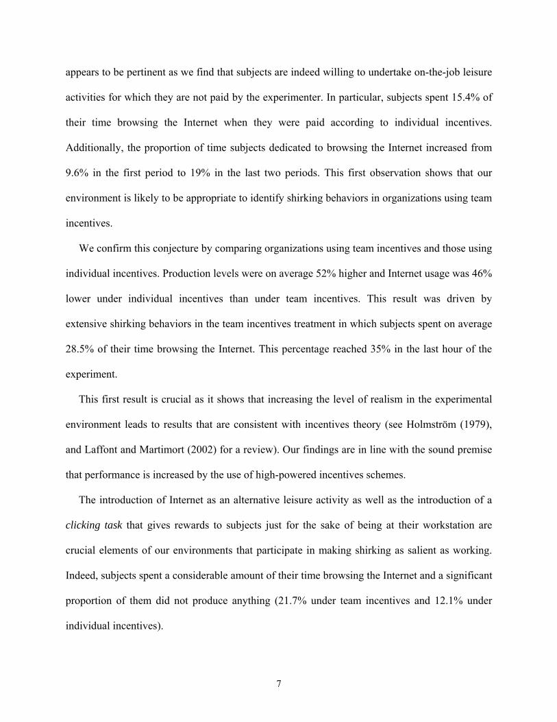
appears to be pertinent as we find that subjects are indeed willing to undertake on-the-job leisure

activities for which they are not paid by the experimenter. In particular, subjects spent 15.4% of

their time browsing the Internet when they were paid according to individual incentives.

Additionally, the proportion of time subjects dedicated to browsing the Internet increased from

9.6% in the first period to 19% in the last two periods. This first observation shows that our

environment is likely to be appropriate to identify shirking behaviors in organizations using team

incentives.

We confirm this conjecture by comparing organizations using team incentives and those using

individual incentives. Production levels were on average 52% higher and Internet usage was 46%

lower under individual incentives than under team incentives. This result was driven by

extensive shirking behaviors in the team incentives treatment in which subjects spent on average

28.5% of their time browsing the Internet. This percentage reached 35% in the last hour of the

experiment.

This first result is crucial as it shows that increasing the level of realism in the experimental

environment leads to results that are consistent with incentives theory (see Holmström (1979),

and Laffont and Martimort (2002) for a review). Our findings are in line with the sound premise

that performance is increased by the use of high-powered incentives schemes.

The introduction of Internet as an alternative leisure activity as well as the introduction of a

clicking task that gives rewards to subjects just for the sake of being at their workstation are

crucial elements of our environments that participate in making shirking as salient as working.

Indeed, subjects spent a considerable amount of their time browsing the Internet and a significant

proportion of them did not produce anything (21.7% under team incentives and 12.1% under

individual incentives).

8

As a second step of our analysis, we introduced a real-time monitoring technology in our

virtual organizations so as to analyze whether the poor performance of team incentives could be

mitigated by peer pressure.

1.3. Supervision and Peer-monitoring in the Theory of Organizations

Supervision is an important aspect of the theory of the firm that was mentioned by preeminent

scholars as one of the raison d'être of organizations (Barzel (1982), Chandler (1992), Jensen and

Meckling (1976)). Alchian and Demsetz (1972) put forward the need for centralized supervision

in a context of asymmetric information between managers and their subordinates in a team

context. The authors argue that supervision should be performed by a residual claimant so as to

provide the monitor with adequate incentives to supervise. By gathering information about the

agents, the monitor will be able to pay employees according to their individual contribution.

Alchian and Demsetz (1972) put forward that peer monitoring is not an efficient mechanism

because the agents would tend to shy away from monitoring activities. However, other theories

view peer monitoring as a highly-effective mechanism (Carpenter, Bowles and Gintis (2009),

Kandel and Lazear (1992)). Kandel and Lazear stress the role of shame arising when workers

produce less than the group average as an important mechanism in understanding the

effectiveness of peer pressure. Carpenter, Bowles and Gintis (2009) emphasize the role of

negative reciprocity as a behavioral mechanism leading contributors to voluntary incur private

costs to punish free riders. Evidence of such behaviors has been found in public good

experiments (Fehr and Gächter (2000), Sefton, Shupp and Walker (2007)). Grosse, Putterman

and Rockenbach (2008) stress the popularity of peer monitoring devices in a modified version of

the public good game. In their experiment, subjects completed a public good game and then

9

decided how much to invest in a monitoring technology which precision determined the

allocation of team profits. The authors found that subjects mostly relied on peer monitoring as a

disciplining device. However, specialist monitoring emerged when the monetary cost of

monitoring by team members was greater than the cost associated with specialist monitoring.

Positive peer effects have been reported in a series of recent field experiments. Falk and

Ichino (2006) found that students who worked for fixed wages to stuff envelopes performed

significantly better when working in pairs than when working alone. Mas and Moretti (2009)

studied the case of supermarket cashiers and found positive peer effects on the number of items

scanned by cashiers. The authors considered workers’ visual contact and frequency of

interactions as measures of peer pressure. In a related field work, Bandiera, Barankay and Rasul

(2005) found that mutual monitoring led fruit pickers to reduce their productivity when they

were paid according to relative performance. The authors interpret this result as evidence of

workers partially internalizing the negative externality of their production on the pay of their co-

workers.

In the field studies described previously, not only did experimenters not have access to precise

measures of peer pressure, they also did not have control over the monitoring process. Peer

pressure was assessed by a variety of observable measures such as visual contact, physical

proximity or frequency of interactions. In this paper, we bring real-time supervision in a

controlled laboratory environment so as to enable the experimenter to measure peer pressure

with precision. In particular, we are able to record the amount of time subjects spent watching

others as well as discern the identity of the subjects who were watching others.

Our peer monitoring technology is characterized by the fact that each team member could

monitor their peers’ activities at any point in time during the experiment. As a result, subjects

10

could shape their monitoring strategy by deciding upon which subjects to monitor and when to

do so.9 Monitors were informed in real-time about the activities undertaken by supervisees and

could therefore identify whether they were browsing the Internet or producing for the

organization. It is important to note that subjects were notified on their screen whenever they

were being watched by others. This feature induced social pressure that is considered to be an

important aspect of peer monitoring (Mas and Moretti (2009)). In that respect, our monitoring

technology was more intrusive than the mere release of feedback about relative performance

introduced in recent experimental works (Blanes i Vidal and Nossol (2011), Eriksson, Poulsen

and Villeval (2009), Kuhnen and Tymula (2009)).10 These studies on feedback are related to

early works in the Psychology literature starting with the development of the social comparison

theory (Festinger (1954)).11 Festinger proposes that individuals try to assess their performance

with respect to others’ when they lack an objective means for evaluation. Upward comparison,

learning that others perform better than one, generally raises motivation as well as effort and

performance (Blanton, Buunk, Gibbons and Kuyper (1999), Seta (1982), Smither, London and

Reilly (2005), Wood (1989)). However, the evidence regarding the effect of feedback on

performance is mixed (Alvero, Bucklin and Austin (2001), Balcazar, Hopkins and Suarez (1985),

Kluger and DeNisi (1996)).12

Our controlled environment offers a single opportunity to provide a detailed analysis of peer

monitoring activities. We first report that a large proportion of subjects (88.3%) decided to

9 This endogenous aspect of our monitoring technology can be linked to search experiments in which subjects decide whether to observe or not their relative performance (Burks et al. (2010), Falk, Huffman and Sunde (2006)). 10 Using both piece-rate and tournament incentive schemes, Eriksson, Poulsen and Villeval (2009) do not report significant effect of feedback on individual performance. Nevertheless, other studies show that social comparison may lead people to exert more effort in tournaments (Kuhnen and Tymula (2009)) or in the context of individual incentives (Blanes i Vidal and Nossol (2011)). The positive effect of feedback in tournaments has been modeled by Kräkel (2008). 11 Extensions of the social comparison theory have been developed (see Suls, Martin and Wheeler (2002) for a review). 12 A significant number of studies find null or even negative effects on performance.

11

monitor others. However, subjects dedicated only a small proportion of their time (4.4%) to

monitoring, compared with the proportion of their time subjects spent working (82.5%) or

browsing the Internet (13.1%). Yet, all subjects were being watched for at least 12 minutes

during the experiment and for an average of 22.4% of their time. Team members seemed to share

the monitoring burden as only 11.7% of them did not supervise their peers at any time. In

addition, subjects spent the same amount of time monitoring others regardless of their

performance on the work task.

We find evidence of strong peer pressure effects when comparing organizations endowed

with peer monitoring and team incentives with organizations relying on team incentives alone.

Production was 50% higher and Internet usage was 54% lower under peer monitoring. In

contrast to public good games with monetary punishments (Carpenter (2007a, 2007b), Fehr and

Gächter (2000)), both effort and efficiency were increased by the introduction of peer

monitoring.13 This was the case because subjects spent little time watching others while sharing

the monitoring burden so as to limit the cost of monitoring.

Peer monitoring combined with team incentives led to levels of performance and Internet

usage that were remarkably similar to individual incentives, despite the absence in our design of

punishments devices, communication technologies or physical proximity among subjects.

Nevertheless, peer pressure was ineffective in raising the production of low performers although

they spent more time working on the task and less time browsing the Internet than in the team

incentives treatment. We relate this result to Zajonc’s social facilitation theory (1965, 1980)

according to which low performers are likely to become more active but less accurate when

being monitored.

13 In public good games, despite the cost of punishments incurred by participants, efficiency may be achieved in the long run (Gächter, Renner and Sefton (2008)).

12

This paper is organized as follows. The experimental design is detailed in the next section

while results are presented in Section III. Concluding remarks are presented in Section IV.

2. EXPERIMENTAL DESIGN

2.1. Virtual Organization With Real Effort and Real Leisure

The core of our methodology is the design of a computerized platform that reproduces crucial

features of real-world work environments. We develop a framework in which subjects can

undertake a real-effort organizational task while having access to Internet at any point in time

during the experiment.14

2.1.1. The Work Task

We introduce a particularly long and laborious task so as to reduce as much as possible the

role of intrinsic motivation in our environment. Indeed, subjects may like certain tasks and derive

direct utility from undertaking the activity. By using a long, repetitive and effortful task we

ensure that individual performance is mostly driven by effort considerations. We do so because

our main objective is to test standard predictions of incentives theory while abstracting from

confounding factors such as intrinsic motivation. The duration of our task as well as its intricacy

were considerably higher than in previous real-effort experiments that have reported the use of

counting tasks (Dohmen and Falk (2011), Eriksson, Poulsen and Villeval (2009), Niederle and

Vesterlund (2007)).15 Subjects were asked to sum up matrices of 36 numbers for 1 hour and 40

14 A video presentation of the software is available at http://sites.google.com/site/virtualorganization/videos. 15 Different variations of this task have been used by Bartling, Fehr, Maréchal and Schunk (2009) and Dohmen and Falk (2010). A counting task that consisted of summing up the number of zeros in a table randomly filled with ones and zeros was also used in Falk and Huffman (2007). A long typing task was used by Dickinson’s (1999) experiment in which subjects had to come during four days for two-hour experiments. Falk and Ichino (2006) used a four-hour mailing task in their field experiment on peer effects.

13

minutes while Niederle and Vesterlund used a 5-minute task and Eriksson, Poulsen and Villeval

used a 20-minute task. The duration of our task was also ten times longer than the multiplication

task used in Dohmen and Falk (2011). As a result, we expected to identify signs of fatigue and

boredom during the experiment.

In the work task, participants were not allowed to use a pen, scratch paper or calculator. This

rule amplified the level of effort subjects had to exert in order to complete tables correctly. Each

table had 6 rows and 6 columns. The numbers in each table were generated randomly. In each

period, the first 5 tables were filled with numbers between 0 and 5 while the following 3 tables

were filled with numbers between 5 and 9. The remaining tables were filled with one-decimal

numbers between 0.0 and 1.0. The increase in the difficulty of the tables was again motivated by

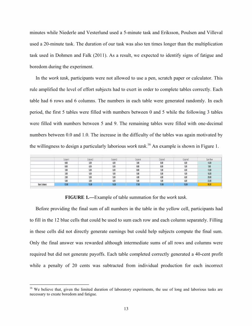
the willingness to design a particularly laborious work task.16 An example is shown in Figure 1.

FIGURE 1.—Example of table summation for the work task.

Before providing the final sum of all numbers in the table in the yellow cell, participants had

to fill in the 12 blue cells that could be used to sum each row and each column separately. Filling

in these cells did not directly generate earnings but could help subjects compute the final sum.

Only the final answer was rewarded although intermediate sums of all rows and columns were

required but did not generate payoffs. Each table completed correctly generated a 40-cent profit

while a penalty of 20 cents was subtracted from individual production for each incorrect

16 We believe that, given the limited duration of laboratory experiments, the use of long and laborious tasks are necessary to create boredom and fatigue.

14

answer.17 After each subject completed a table, the accumulated individual production was

updated so that subjects knew whether their answer was correct or not. At the end of each period,

and only then, the total amount of money generated by all 10 participants’ work task during the

period was displayed in the history panel located at the bottom of the subjects’ screen.

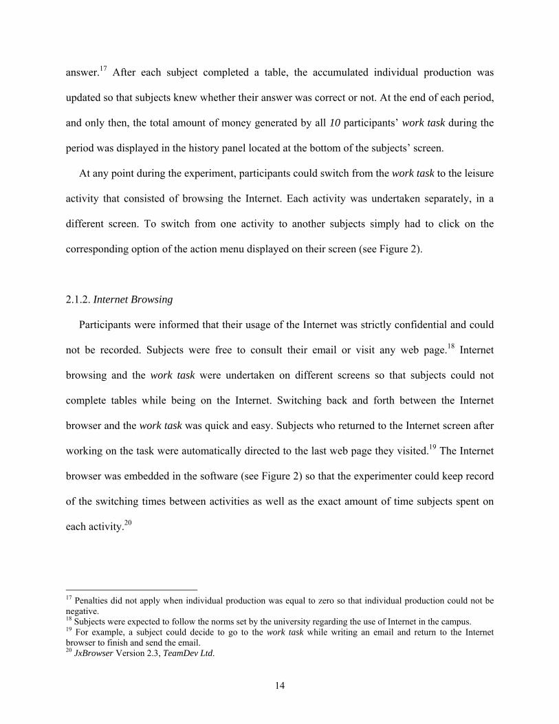
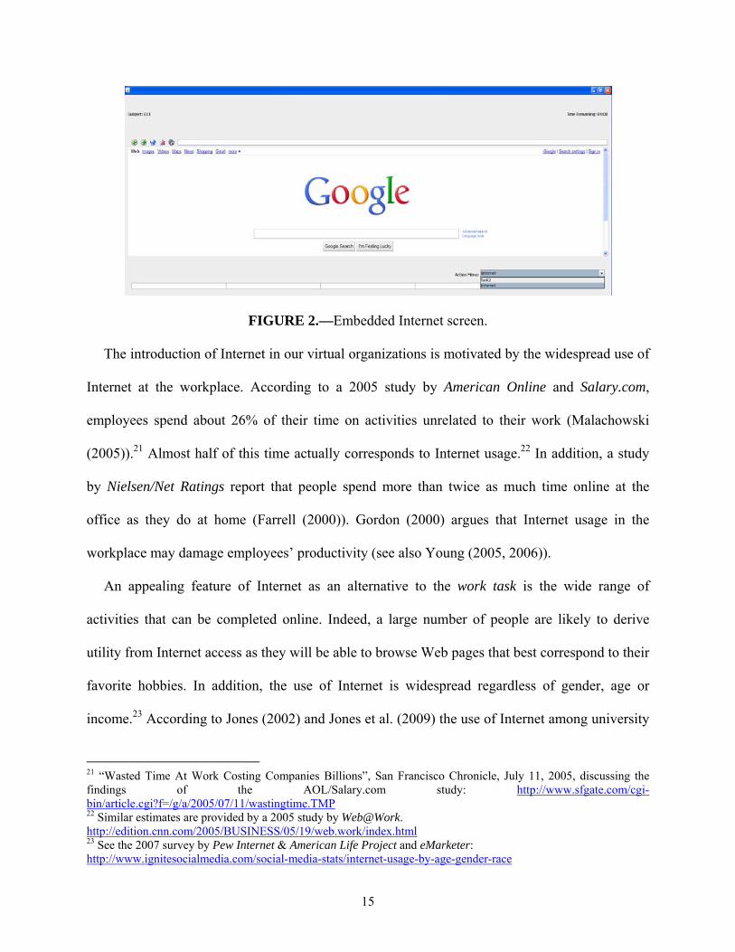
At any point during the experiment, participants could switch from the work task to the leisure

activity that consisted of browsing the Internet. Each activity was undertaken separately, in a

different screen. To switch from one activity to another subjects simply had to click on the

corresponding option of the action menu displayed on their screen (see Figure 2).

2.1.2. Internet Browsing

Participants were informed that their usage of the Internet was strictly confidential and could

not be recorded. Subjects were free to consult their email or visit any web page.18 Internet

browsing and the work task were undertaken on different screens so that subjects could not

complete tables while being on the Internet. Switching back and forth between the Internet

browser and the work task was quick and easy. Subjects who returned to the Internet screen after

working on the task were automatically directed to the last web page they visited.19 The Internet

browser was embedded in the software (see Figure 2) so that the experimenter could keep record

of the switching times between activities as well as the exact amount of time subjects spent on

each activity.20

17 Penalties did not apply when individual production was equal to zero so that individual production could not be negative. 18 Subjects were expected to follow the norms set by the university regarding the use of Internet in the campus. 19 For example, a subject could decide to go to the work task while writing an email and return to the Internet browser to finish and send the email. 20 JxBrowser Version 2.3, TeamDev Ltd.

15

FIGURE 2.—Embedded Internet screen.

The introduction of Internet in our virtual organizations is motivated by the widespread use of

Internet at the workplace. According to a 2005 study by American Online and Salary.com,

employees spend about 26% of their time on activities unrelated to their work (Malachowski

(2005)).21 Almost half of this time actually corresponds to Internet usage.22 In addition, a study

by Nielsen/Net Ratings report that people spend more than twice as much time online at the

office as they do at home (Farrell (2000)). Gordon (2000) argues that Internet usage in the

workplace may damage employees’ productivity (see also Young (2005, 2006)).

An appealing feature of Internet as an alternative to the work task is the wide range of

activities that can be completed online. Indeed, a large number of people are likely to derive

utility from Internet access as they will be able to browse Web pages that best correspond to their

favorite hobbies. In addition, the use of Internet is widespread regardless of gender, age or

income.23 According to Jones (2002) and Jones et al. (2009) the use of Internet among university

21 “Wasted Time At Work Costing Companies Billions”, San Francisco Chronicle, July 11, 2005, discussing the findings of the AOL/Salary.com study: http://www.sfgate.com/cgi-bin/article.cgi?f=/g/a/2005/07/11/wastingtime.TMP 22 Similar estimates are provided by a 2005 study by Web@Work. http://edition.cnn.com/2005/BUSINESS/05/19/web.work/index.html 23 See the 2007 survey by Pew Internet & American Life Project and eMarketer: http://www.ignitesocialmedia.com/social-media-stats/internet-usage-by-age-gender-race

16

students has increased significantly in the last years. Jones et al. (2009) found that 94% of

college students spend at least one hour on the Internet every day, and 53% spend three or more

hours.24 Furthermore, Internet is not restricted to a specific kind of leisure as opposed to simply

playing a video game, reading a newspaper or listening to music. All of these activities and more

are available through the Internet. Looking at the most visited Web sites by college students

gives us an idea of the great variety of options available on the Internet.25 In addition, Jones et al.

(2009) find that students access the Internet several times during the day and at nonspecific

times.

Furthermore, devising environments that include features of real-world organizations such as

on-the-job Internet usage may reduce demand effects in the laboratory (Zizzo (2010)).26 Indeed,

the use of Internet as an alternative activity as well may lead people to consider that shirking is

an equally salient alternative to working.

The consideration of leisure-related issues in the experimental literature was introduced in the

analysis of labor supply by Dickinson (1999). The objective of the author was to assess both

income and substitution effects using laboratory experiments. Participants had to undertake a

two-hour typing task on three different days. In one of the two treatments (the combined

experiment), subjects could leave the laboratory whenever they had achieved a certain output

level. This aimed at capturing off-the-job leisure activities. Falk and Huffman (2007) also

24 Harris Interactive’s “360 College Explorer Outlook Study” in 2002 found that Internet is the most common activity among students, with 98% of students going online at least a few times a week, and spending on average almost 10 hours per week on the Net (http://www.harrisinteractive.com/news/allnewsbydate.asp?NewsID=441). 25 The ten most visited Web sites are Facebook, ESPN, Google, CNN, YouTube, MSN, Hulu, StumbleUpon, Pandora and Craiglist for male students and Facebook, Google, Yahoo!, PerezHilton.com, MySpace, School’s site, CNN, AOL, eBay and The Superficial for college girls (Youth Trends, “The Top Ten List Report: College Q3 2008,” http://ldsmediatalk.com/2009/02/16/internet-use-among-teens-vs-college-students/). 26 In addition, subjects faced computerized instructions and were not interacting with the experimenter except for the unlikely case in which questions were raised by subjects. The great majority of subjects (we estimate this proportion to be around 95%) would typically never ask questions. We think this is partly explained by the intuitive structure of our environment.

17

introduced the possibility for subjects to quit the experiment when analyzing minimum wages

and workfare in the laboratory. However, it is difficult to interpret the heterogeneity in quitting

behaviors given the lack of control over subjects’ activities outside the laboratory. Ours is the

first experimental design that embeds on-the-job leisure activities into the work environment and

that allows the experimenter to measure the exact amount of time each subject spent on leisure

and work activities.27

2.1.3. The Clicking Task

In addition to the previously mentioned activities, each subject could click on a yellow box

moving from left to right at the bottom of their screen. This task was referred to as Task 1. Each

time a subject clicked on the yellow box he or she earned 5 cents. Subjects’ earnings obtained

from clicking the box were displayed on the screen and updated each time they clicked on the

yellow box. The box appeared at the bottom of a subject’s screen every 25 seconds whether a

subject was on the work task or browsing the Internet. The yellow box always appeared first on

the left hand side of the screen, and moved to the right (see Figure 3). It remained during 4

seconds in the first cell on the left and then moved to the next cell for another 4 seconds if the

subject had not clicked on the box. This means that the box was visible on the screen for a total

of 20 seconds or until a subject clicked on it. Given that the experiment consisted of 5 periods of

20 minutes each, subjects could earn a total of $12.00 just by clicking on all the 240 yellow

boxes that appeared on the screen during the experiment.

27 Two related studies (Charness, Masclet and Villeval (2010), Eriksson, Poulsen and Villeval (2009)) have also introduced on-the-job leisure activities in experimental environments by giving subjects access to magazines. However, the leisure activity was not embedded in the computerized platform.

18

FIGURE 3.—The clicking task.

This task aimed at representing the pay that workers may obtain just for being at their

workstation. One can see this activity as a way to endogenize the show-up fee.28 A crucial

motivation for the introduction of the clicking task was to add realism to our experimental design

by allowing subjects to collect a constant flow of earnings without being actually working. In

each period, subjects could earn up to $2.40 by clicking on the yellow boxes.

2.2. Virtual Organization: Real-time Monitoring

Another crucial feature of our experimental environement is the introduction of real-time

supervision. In the peer monitoring treatment, subjects were able monitor others’ activities in

real time. Our objective was to design an environment that allows for the emergence of peer

effects that were defined by Charness and Kuhn (2011) as follows: “…pure peer effects refer to a

situation where workers work, side by side, for the same firm but do not interact in any way

(except that they observe each others’ work activity).”

To that end, we allowed subjects to monitor others’ activities at any time during the

experiment by selecting the Watch option in their action menu. In that respect, our monitoring

technology offered a unique opportunity to assess the effect of peer pressure over time and

examine the conjecture that peer effects are likely to fade away as time passes (Falk and Ichino

(2006)).

28 Notice that subjects were also paid the standard laboratory show-up fee of $7.

19

Monitoring activities had to be undertaken in a separate screen so that subjects could not

complete the work task or the leisure activity while monitoring others.29 As a result, monitoring

imposed an opportunity cost on watchers that was different in nature from the monetary cost of

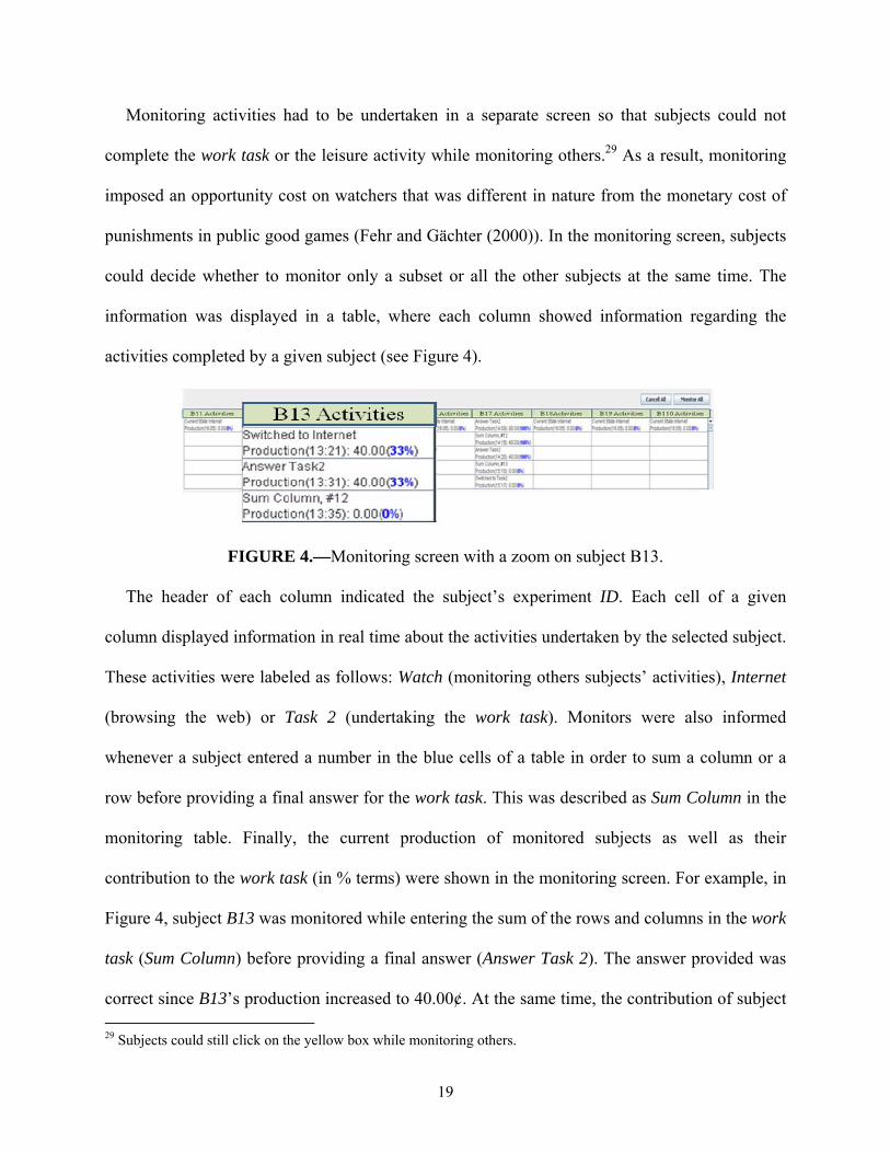
punishments in public good games (Fehr and Gächter (2000)). In the monitoring screen, subjects

could decide whether to monitor only a subset or all the other subjects at the same time. The

information was displayed in a table, where each column showed information regarding the

activities completed by a given subject (see Figure 4).

FIGURE 4.—Monitoring screen with a zoom on subject B13.

The header of each column indicated the subject’s experiment ID. Each cell of a given

column displayed information in real time about the activities undertaken by the selected subject.

These activities were labeled as follows: Watch (monitoring others subjects’ activities), Internet

(browsing the web) or Task 2 (undertaking the work task). Monitors were also informed

whenever a subject entered a number in the blue cells of a table in order to sum a column or a

row before providing a final answer for the work task. This was described as Sum Column in the

monitoring table. Finally, the current production of monitored subjects as well as their

contribution to the work task (in % terms) were shown in the monitoring screen. For example, in

Figure 4, subject B13 was monitored while entering the sum of the rows and columns in the work

task (Sum Column) before providing a final answer (Answer Task 2). The answer provided was

correct since B13’s production increased to 40.00¢. At the same time, the contribution of subject 29 Subjects could still click on the yellow box while monitoring others.

20

B13 to the work task increased from nothing to one-third. Notice that after completing the table

correctly, subject B13 switched to the Internet screen with 13 minutes and 21 seconds remaining

in the period.

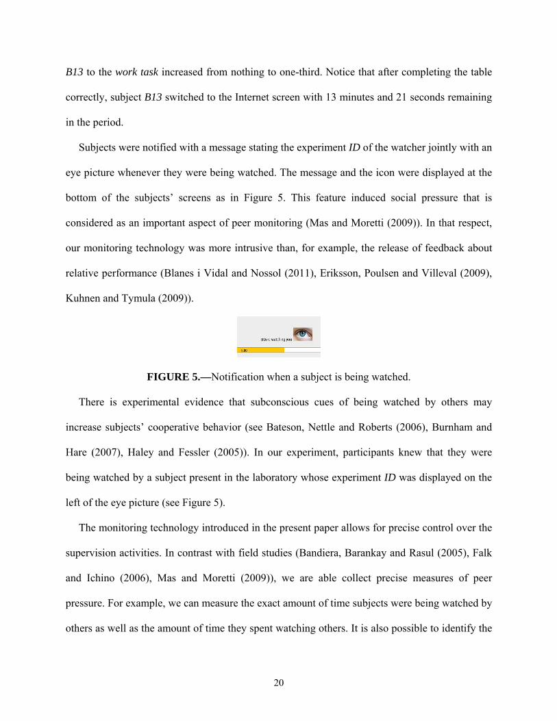
Subjects were notified with a message stating the experiment ID of the watcher jointly with an

eye picture whenever they were being watched. The message and the icon were displayed at the

bottom of the subjects’ screens as in Figure 5. This feature induced social pressure that is

considered as an important aspect of peer monitoring (Mas and Moretti (2009)). In that respect,

our monitoring technology was more intrusive than, for example, the release of feedback about

relative performance (Blanes i Vidal and Nossol (2011), Eriksson, Poulsen and Villeval (2009),

Kuhnen and Tymula (2009)).

FIGURE 5.—Notification when a subject is being watched.

There is experimental evidence that subconscious cues of being watched by others may

increase subjects’ cooperative behavior (see Bateson, Nettle and Roberts (2006), Burnham and

Hare (2007), Haley and Fessler (2005)). In our experiment, participants knew that they were

being watched by a subject present in the laboratory whose experiment ID was displayed on the

left of the eye picture (see Figure 5).

The monitoring technology introduced in the present paper allows for precise control over the

supervision activities. In contrast with field studies (Bandiera, Barankay and Rasul (2005), Falk

and Ichino (2006), Mas and Moretti (2009)), we are able collect precise measures of peer

pressure. For example, we can measure the exact amount of time subjects were being watched by

others as well as the amount of time they spent watching others. It is also possible to identify the

21

watchers as well as the subjects who were being watched. Finally, the experimenter has access to

the information that was displayed on the watchers’ screens at a given time. This information can

be used in the analysis of peer monitoring effects.

Another distinctive feature of our monitoring technology is that subjects could freely decide

upon their monitoring strategy. Subjects could choose who to monitor and when to do so. This

feature of the supervision technology will allow us to analyze subjects’ monitoring strategies.

2.3. Treatments & Hypotheses

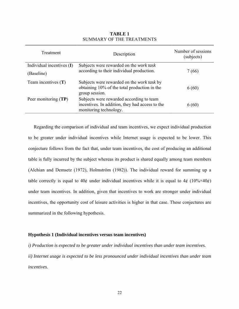
We ran three different treatments (see Table 1). In the baseline treatment, subjects were

rewarded on the work task according to their individual production. We refer to this case as

Treatment I for individual incentives. In the second treatment, team incentives (Treatment T), the

total production of the 10 subjects participating in the experiment was equally distributed among

them. Our third experiment was the peer monitoring treatment (Treatment TP). Treatment TP

was equivalent to Treatment T except that subjects could monitor their peers using the

technology described in the previous section. The instructions for each treatment are available

online.30In order to establish predictions regarding the comparison of production levels and

Internet usage across treatments, we rely on standard incentives theory (see Laffont and

Martimort (2002) for a review). We voluntarily discard behavioral aspects such as social

preferences (Fehr and Shmidt (1999)) in establishing those predictions. This is motivated by the

fact that standard incentives theory leads to a unique set of predictions while introducing

behavioral considerations may lead to multiple conjectures.

30 http://sites.google.com/site/virtualorganization/instructions.

22

TABLE 1 SUMMARY OF THE TREATMENTS

Treatment Description Number of sessions (subjects)

Individual incentives (I)

(Baseline)

Subjects were rewarded on the work task according to their individual production. 7 (66)

Team incentives (T) Subjects were rewarded on the work task by obtaining 10% of the total production in the group session.

6 (60)

Peer monitoring (TP) Subjects were rewarded according to team incentives. In addition, they had access to the monitoring technology.

6 (60)

Regarding the comparison of individual and team incentives, we expect individual production

to be greater under individual incentives while Internet usage is expected to be lower. This

conjecture follows from the fact that, under team incentives, the cost of producing an additional

table is fully incurred by the subject whereas its product is shared equally among team members

(Alchian and Demsetz (1972), Holmström (1982)). The individual reward for summing up a

table correctly is equal to 40¢ under individual incentives while it is equal to 4¢ (10%×40¢)

under team incentives. In addition, given that incentives to work are stronger under individual

incentives, the opportunity cost of leisure activities is higher in that case. These conjectures are

summarized in the following hypothesis.

Hypothesis 1 (Individual incentives versus team incentives)

i) Production is expected to be greater under individual incentives than under team incentives.

ii) Internet usage is expected to be less pronounced under individual incentives than under team

incentives.

23

Introducing behavioral considerations, we may also expect, in line with previous research,

that team incentives will perform as well as individual incentives as a result of team spirit or

team identity and interpersonal relationships among team members (Dumaine (1990, 1994),

Hamilton, Nickerson and Owan (2003), Hansen (1997), Ichniowski et al. (1996), Ichniowski,

Shaw and Prennushi (1997), Kruse (1992), Manz and Sims (1993), van Dijk, Sonnemans and van

Winden (2001)). However, none of these relevant features were introduced explicitly in our

design.

Regarding the comparison of the team incentives and the peer pressure treatments, standard

incentives theory would predict no differences both in terms of production and Internet usage. In

contrast with the work task, subjects had no monetary incentives to monitor others. Peer

monitoring was a time consuming activity either in terms of work time or in terms of leisure

time. As long as we ignore behavioral considerations, we should expect subjects to shy away

from monitoring activities because they constituted a less attractive option than either working

for cash or browsing the Internet. As a result, we should expect Treatment T and Treatment TP to

be equivalent and lead to similar production levels as well as similar Internet usage. This

conjecture is stated in the following hypothesis.

Hypothesis 2 (Peer monitoring)

Production as well as Internet usage are expected to be similar for the team incentives and the

peer pressure treatments.

Considering behavioral aspects may lead to different predictions. For example, one may

believe that people use monitoring as a tool to foster peer pressure and increase production as a

24

result (Carpenter, Bowles and Gintis (2009) and Kandel and Lazear (1992)). At the same time,

one may expect monitoring activities to backfire generating distrust among workers. Indeed,

recent research has emphasized this negative aspect of monitoring and put forward that trusting

employees can lead to higher levels of effort than intensive supervision (Dickinson and Villeval

(2008), Falk and Kosfeld (2006), Fehr, Klein and Schmidt (2007a, 2007b), Frey (1993)).31 We

do not consider crowding-out of effort as our primary hypothesis because the disciplining effect

of supervision has been found to be dominant in the absence of interpersonal relationships

among workers as is the case in our experimental design (Dickinson and Villeval (2008), Frey

(1993)). In addition, crowding-out effects are likely to be stronger in a principal-agent

relationship or in any situation in which the monitor has some authority on the supervisee’s

work. In our design, we consider a multi-agent monitoring structure in which there is no

principal and no hierarchy since each subject has the same role.

2.4. Procedures

Our subject pool consisted of students from Chapman University. The experiments took place

in December 2010 and February 2011. In total, 186 subjects participated in the experiment,

divided in 17 sessions. We ran seven sessions for Treatment I, and six sessions for each of

Treatments T and TP. Ten students participated in each session, except for two sessions of 8

students that corresponded to Treatment I. The experiment was computerized using the software

Virtual Organizations developed by CYDeveloper LLC. All of the interaction was anonymous.

The instructions were displayed on subjects’ computer screen whenever all of them were

seated. Subjects had exactly 20 minutes to read the instructions. A 20-minute timer was shown

31 Crowding-out of intrinsic motivation has also been studied in the Psychology literature (Deci (1971, 1975), Deci, Koestner and Ryan (1999)). A theoretical account of crowding-out of intrinsic motivation has been provided by Bénabou and Tirole (2003).

25

on the laboratory screen. Three minutes before the end of the instructions period, a monitor

entered into the room announcing the time remaining and handing out a printed copy of the

summary of the instructions. None of the participants asked for extra time to read the

instructions.32 At the end of the 20-minute instruction round, the experimenter closed the

instructions file from the server, and subjects typed their names to start the experiment. The

interaction between the experimenter and the participants was negligible. We estimate that only

5% of the subjects raised a question during the instructions period, and only very few subjects

asked questions during the experiment.33

At the end of the experiment, all subjects were paid their earnings in cash, rounded up to the

nearest quarter. Individual earnings at the end of the experiment are computed as the sum of the

earnings in the 5 periods. Participants earned on average $26.30, including a $7.00 show-up fee.

Participants in Treatments I, T, and TP, earned on average $27.25, $24.45, and $27.10,

respectively. Experimental sessions lasted on average two hours and ten minutes.

3. RESULTS

We start the results section by presenting a detailed analysis of the individual incentives

treatment that will serve as a benchmark for our subsequent analyses. The team incentives

treatment is analyzed in Section 3.2 and the peer pressure treatment is studied in Section 3.3. In

Section 3.4, we assess the effect of each treatment on high-, middle-, and low- performers

separately.

32 At the time the monitor entered the room, most participants had already finished reading the instructions and were waiting the experiment to start. 33 In the majority of sessions, no questions were asked during the experiment.

26

3.1. Individual Incentives

3.1.1. The Work Task and the Clicking Task

In this section we analyze the data that correspond to Treatment I (individual incentives) in

which subjects were rewarded according to their individual production on the work task (Task 2).

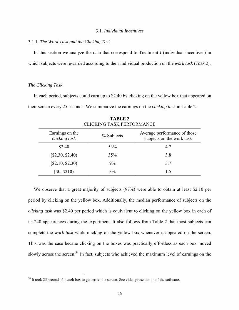
The Clicking Task

In each period, subjects could earn up to $2.40 by clicking on the yellow box that appeared on

their screen every 25 seconds. We summarize the earnings on the clicking task in Table 2.

TABLE 2 CLICKING TASK PERFORMANCE

Earnings on the clicking task % Subjects Average performance of those

subjects on the work task

$2.40 53% 4.7

[$2.30, $2.40) 35% 3.8

[$2.10, $2.30) 9% 3.7

[$0, $210) 3% 1.5

We observe that a great majority of subjects (97%) were able to obtain at least $2.10 per

period by clicking on the yellow box. Additionally, the median performance of subjects on the

clicking task was $2.40 per period which is equivalent to clicking on the yellow box in each of

its 240 appearences during the experiment. It also follows from Table 2 that most subjects can

complete the work task while clicking on the yellow box whenever it appeared on the screen.

This was the case becaue clicking on the boxes was practically effortless as each box moved

slowly across the screen.34 In fact, subjects who achieved the maximum level of earnings on the

34 It took 25 seconds for each box to go across the screen. See video presentation of the software.

27

clicking task ($2.40) obtained significantly larger earnings on the work task than other subjects

(Wilcoxon rank-sum test, p = 0.05).35

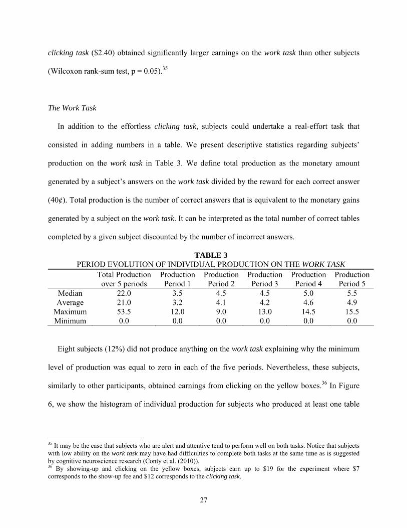
The Work Task

In addition to the effortless clicking task, subjects could undertake a real-effort task that

consisted in adding numbers in a table. We present descriptive statistics regarding subjects’

production on the work task in Table 3. We define total production as the monetary amount

generated by a subject’s answers on the work task divided by the reward for each correct answer

(40¢). Total production is the number of correct answers that is equivalent to the monetary gains

generated by a subject on the work task. It can be interpreted as the total number of correct tables

completed by a given subject discounted by the number of incorrect answers.

TABLE 3 PERIOD EVOLUTION OF INDIVIDUAL PRODUCTION ON THE WORK TASK

Total Production over 5 periods

Production Period 1

Production Period 2

Production Period 3

Production Period 4

Production Period 5

Median 22.0 3.5 4.5 4.5 5.0 5.5 Average 21.0 3.2 4.1 4.2 4.6 4.9

Maximum 53.5 12.0 9.0 13.0 14.5 15.5 Minimum 0.0 0.0 0.0 0.0 0.0 0.0

Eight subjects (12%) did not produce anything on the work task explaining why the minimum

level of production was equal to zero in each of the five periods. Nevertheless, these subjects,

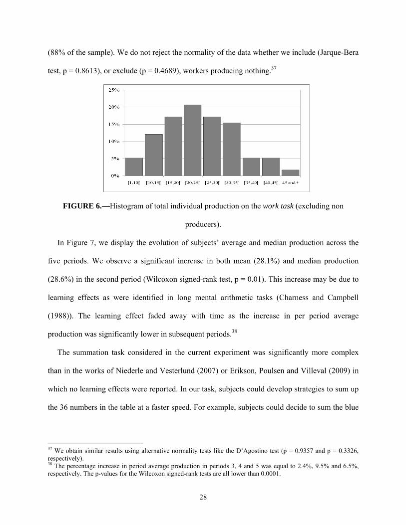
similarly to other participants, obtained earnings from clicking on the yellow boxes.36 In Figure

6, we show the histogram of individual production for subjects who produced at least one table

35 It may be the case that subjects who are alert and attentive tend to perform well on both tasks. Notice that subjects with low ability on the work task may have had difficulties to complete both tasks at the same time as is suggested by cognitive neuroscience research (Conty et al. (2010)). 36 By showing-up and clicking on the yellow boxes, subjects earn up to $19 for the experiment where $7 corresponds to the show-up fee and $12 corresponds to the clicking task.

28

(88% of the sample). We do not reject the normality of the data whether we include (Jarque-Bera

test, p = 0.8613), or exclude (p = 0.4689), workers producing nothing.37

FIGURE 6.—Histogram of total individual production on the work task (excluding non

producers).

In Figure 7, we display the evolution of subjects’ average and median production across the

five periods. We observe a significant increase in both mean (28.1%) and median production

(28.6%) in the second period (Wilcoxon signed-rank test, p = 0.01). This increase may be due to

learning effects as were identified in long mental arithmetic tasks (Charness and Campbell

(1988)). The learning effect faded away with time as the increase in per period average

production was significantly lower in subsequent periods.38

The summation task considered in the current experiment was significantly more complex

than in the works of Niederle and Vesterlund (2007) or Erikson, Poulsen and Villeval (2009) in

which no learning effects were reported. In our task, subjects could develop strategies to sum up

the 36 numbers in the table at a faster speed. For example, subjects could decide to sum the blue

37 We obtain similar results using alternative normality tests like the D’Agostino test (p = 0.9357 and p = 0.3326, respectively). 38 The percentage increase in period average production in periods 3, 4 and 5 was equal to 2.4%, 9.5% and 6.5%, respectively. The p-values for the Wilcoxon signed-rank tests are all lower than 0.0001.

29

cells (that could be used to sum rows and columns) with arbitrary numbers and compute only the

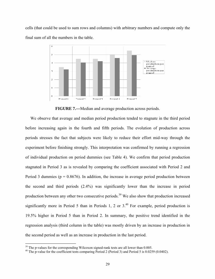
final sum of all the numbers in the table.

FIGURE 7.—Median and average production across periods.

We observe that average and median period production tended to stagnate in the third period

before increasing again in the fourth and fifth periods. The evolution of production across

periods stresses the fact that subjects were likely to reduce their effort mid-way through the

experiment before finishing strongly. This interpretation was confirmed by running a regression

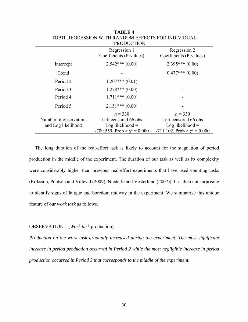
of individual production on period dummies (see Table 4). We confirm that period production

stagnated in Period 3 as is revealed by comparing the coefficient associated with Period 2 and

Period 3 dummies (p = 0.8676). In addition, the increase in average period production between

the second and third periods (2.4%) was significantly lower than the increase in period

production between any other two consecutive periods.39 We also show that production increased

significantly more in Period 5 than in Periods 1, 2 or 3.40 For example, period production is

19.5% higher in Period 5 than in Period 2. In summary, the positive trend identified in the

regression analysis (third column in the table) was mostly driven by an increase in production in

the second period as well as an increase in production in the last period.

39 The p-values for the corresponding Wilcoxon signed-rank tests are all lower than 0.005. 40 The p-value for the coefficient tests comparing Period 2 (Period 3) and Period 5 is 0.0259 (0.0402).

30

TABLE 4 TOBIT REGRESSION WITH RANDOM EFFECTS FOR INDIVIDUAL

PRODUCTION

Regression 1 Coefficients (P-values)


Intercept 2.542*** (0.00) 2.395*** (0.00)

Trend - 0.477*** (0.00)

Period 2 1.207*** (0.01) -

Period 3 1.278*** (0.00) - Period 4 1.711*** (0.00) -

Period 5 2.151*** (0.00) -

Number of observations and Log likelihood

n = 330 Left censored 66 obs

Log likelihood = -709.559, Prob > χ² = 0.000



The long duration of the real-effort task is likely to account for the stagnation of period

production in the middle of the experiment. The duration of our task as well as its complexity

were considerably higher than previous real-effort experiments that have used counting tasks

(Eriksson, Poulsen and Villeval (2009), Niederle and Vesterlund (2007)). It is then not surprising

to identify signs of fatigue and boredom midway in the experiment. We summarize this unique

feature of our work task as follows.

OBSERVATION 1 (Work task production)

Production on the work task gradually increased during the experiment. The most significant

increase in period production occurred in Period 2 while the most negligible increase in period

production occurred in Period 3 that corresponds to the middle of the experiment.

31

In addition to the work task and the clicking task, subjects also had access to real-leisure

activities. Subjects could browse the Internet at any time during the experiment by switching to

the Internet screen using the action menu. Browsing activities are analyzed in the following

section.

3.1.2. Working or Browsing the Internet

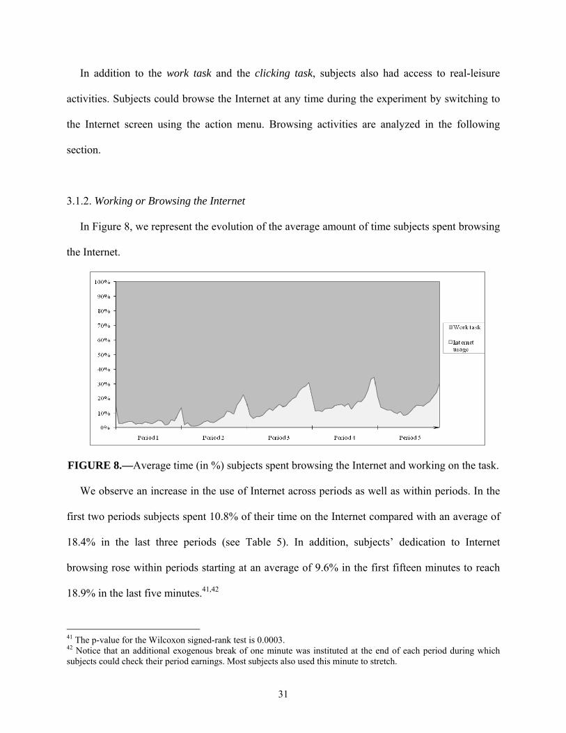
In Figure 8, we represent the evolution of the average amount of time subjects spent browsing

the Internet.

FIGURE 8.—Average time (in %) subjects spent browsing the Internet and working on the task.

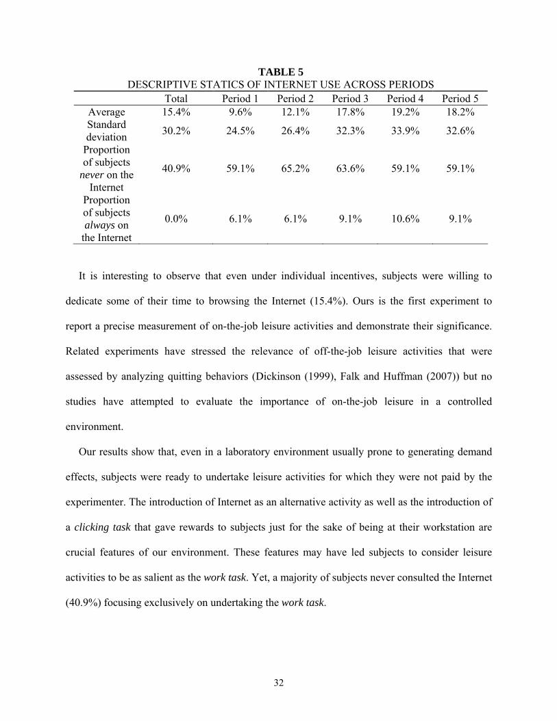
We observe an increase in the use of Internet across periods as well as within periods. In the

first two periods subjects spent 10.8% of their time on the Internet compared with an average of

18.4% in the last three periods (see Table 5). In addition, subjects’ dedication to Internet

browsing rose within periods starting at an average of 9.6% in the first fifteen minutes to reach

18.9% in the last five minutes.41,42

41 The p-value for the Wilcoxon signed-rank test is 0.0003. 42 Notice that an additional exogenous break of one minute was instituted at the end of each period during which subjects could check their period earnings. Most subjects also used this minute to stretch.

32

TABLE 5 DESCRIPTIVE STATICS OF INTERNET USE ACROSS PERIODS

Total Period 1 Period 2 Period 3 Period 4 Period 5 Average 15.4% 9.6% 12.1% 17.8% 19.2% 18.2% Standard deviation 30.2% 24.5% 26.4% 32.3% 33.9% 32.6%

Proportion of subjects

never on the Internet

40.9% 59.1% 65.2% 63.6% 59.1% 59.1%

Proportion of subjects always on

the Internet

0.0% 6.1% 6.1% 9.1% 10.6% 9.1%

It is interesting to observe that even under individual incentives, subjects were willing to

dedicate some of their time to browsing the Internet (15.4%). Ours is the first experiment to

report a precise measurement of on-the-job leisure activities and demonstrate their significance.

Related experiments have stressed the relevance of off-the-job leisure activities that were

assessed by analyzing quitting behaviors (Dickinson (1999), Falk and Huffman (2007)) but no

studies have attempted to evaluate the importance of on-the-job leisure in a controlled

environment.

Our results show that, even in a laboratory environment usually prone to generating demand

effects, subjects were ready to undertake leisure activities for which they were not paid by the

experimenter. The introduction of Internet as an alternative activity as well as the introduction of

a clicking task that gave rewards to subjects just for the sake of being at their workstation are

crucial features of our environment. These features may have led subjects to consider leisure

activities to be as salient as the work task. Yet, a majority of subjects never consulted the Internet

(40.9%) focusing exclusively on undertaking the work task.

33

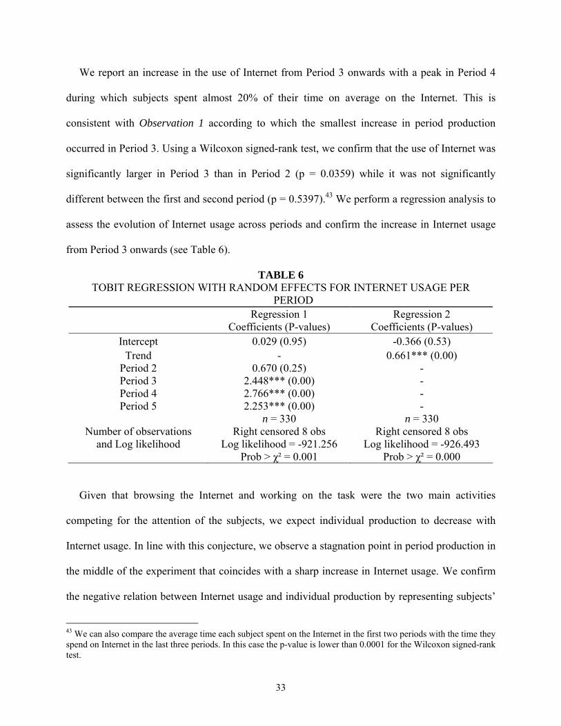
We report an increase in the use of Internet from Period 3 onwards with a peak in Period 4

during which subjects spent almost 20% of their time on average on the Internet. This is

consistent with Observation 1 according to which the smallest increase in period production

occurred in Period 3. Using a Wilcoxon signed-rank test, we confirm that the use of Internet was

significantly larger in Period 3 than in Period 2 (p = 0.0359) while it was not significantly

different between the first and second period (p = 0.5397).43 We perform a regression analysis to

assess the evolution of Internet usage across periods and confirm the increase in Internet usage

from Period 3 onwards (see Table 6).

TABLE 6 TOBIT REGRESSION WITH RANDOM EFFECTS FOR INTERNET USAGE PER

PERIOD



Intercept 0.029 (0.95) -0.366 (0.53) Trend - 0.661*** (0.00)

Period 2 0.670 (0.25) - Period 3 2.448*** (0.00) - Period 4 2.766*** (0.00) - Period 5 2.253*** (0.00) -


n = 330 Right censored 8 obs

Log likelihood = -921.256 Prob > χ² = 0.001


Log likelihood = -926.493 Prob > χ² = 0.000

Given that browsing the Internet and working on the task were the two main activities

competing for the attention of the subjects, we expect individual production to decrease with

Internet usage. In line with this conjecture, we observe a stagnation point in period production in

the middle of the experiment that coincides with a sharp increase in Internet usage. We confirm

the negative relation between Internet usage and individual production by representing subjects’

43 We can also compare the average time each subject spent on the Internet in the first two periods with the time they spend on Internet in the last three periods. In this case the p-value is lower than 0.0001 for the Wilcoxon signed-rank test.

34

average production for increasing ranges of Internet usage (see Figure A.1 in the appendix). In

addition, we report that the correlation between Internet usage and individual production was

negative and significant regardless of the methodology used to compute correlation

coefficients.44

One should not misinterpret the positive trend in both production and Internet usage as

evidence of a positive relationship between work performance and leisure. Instead, one should

recognize that the positive trend in production is mostly driven by learning effects that are

unrelated to Internet usage.45

OBSERVATION 2 (Internet usage)

i) The use of Internet started to increase significantly in the third period.

ii) The use of Internet rose sharply in the last five minutes of each period.

ii) The use of Internet was negatively correlated with individual production.

In the next section, we compare individual incentives with team incentives in terms of

production and Internet usage. The comparison between individual and team incentives

constitutes an important step in our understanding of the role of incentives in the virtual

organizations introduced in the present paper.

44 The Pearson (Spearman) [Kendall] coefficient is equal to -0.5506 (-0.3783) [-0.2687] with p < 0.0001 (p = 0.0017) [p = 0.0016]. 45 In other words, we expect the positive trend in production to be steeper in the absence of Internet usage.

35

3.2. Team Incentives Versus Individual Incentives

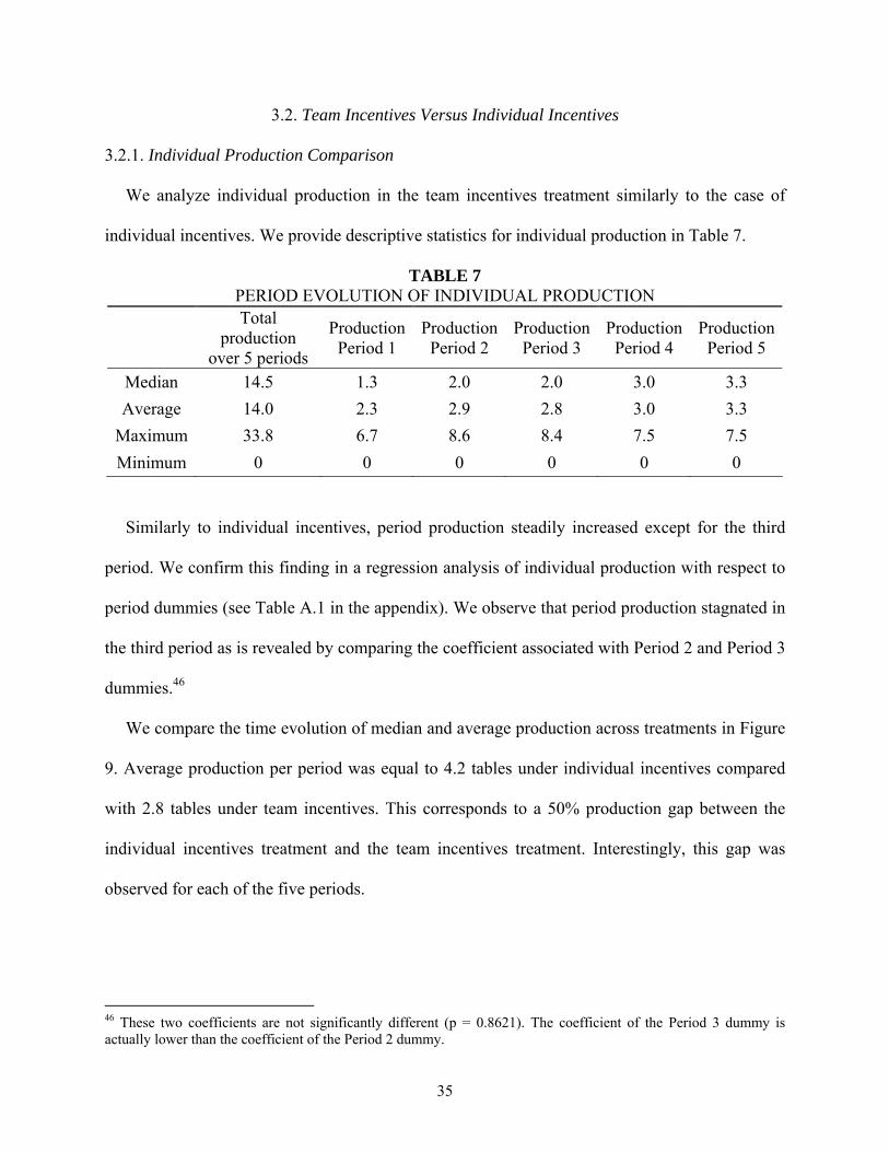
3.2.1. Individual Production Comparison

We analyze individual production in the team incentives treatment similarly to the case of

individual incentives. We provide descriptive statistics for individual production in Table 7.

TABLE 7 PERIOD EVOLUTION OF INDIVIDUAL PRODUCTION

Total

production over 5 periods

Production Period 1

Production Period 2

Production Period 3

Production Period 4

Production Period 5

Median 14.5 1.3 2.0 2.0 3.0 3.3 Average 14.0 2.3 2.9 2.8 3.0 3.3

Maximum 33.8 6.7 8.6 8.4 7.5 7.5 Minimum 0 0 0 0 0 0

Similarly to individual incentives, period production steadily increased except for the third

period. We confirm this finding in a regression analysis of individual production with respect to

period dummies (see Table A.1 in the appendix). We observe that period production stagnated in

the third period as is revealed by comparing the coefficient associated with Period 2 and Period 3

dummies.46

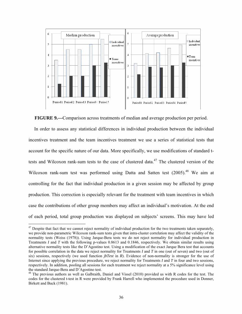
We compare the time evolution of median and average production across treatments in Figure

9. Average production per period was equal to 4.2 tables under individual incentives compared

with 2.8 tables under team incentives. This corresponds to a 50% production gap between the

individual incentives treatment and the team incentives treatment. Interestingly, this gap was

observed for each of the five periods.

46 These two coefficients are not significantly different (p = 0.8621). The coefficient of the Period 3 dummy is actually lower than the coefficient of the Period 2 dummy.

36

FIGURE 9.—Comparison across treatments of median and average production per period.

In order to assess any statistical differences in individual production between the individual

incentives treatment and the team incentives treatment we use a series of statistical tests that

account for the specific nature of our data. More specifically, we use modifications of standard t-

tests and Wilcoxon rank-sum tests to the case of clustered data.47 The clustered version of the

Wilcoxon rank-sum test was performed using Datta and Satten test (2005).48 We aim at

controlling for the fact that individual production in a given session may be affected by group

production. This correction is especially relevant for the treatment with team incentives in which

case the contributions of other group members may affect an individual’s motivation. At the end

of each period, total group production was displayed on subjects’ screens. This may have led 47 Despite that fact that we cannot reject normality of individual production for the two treatments taken separately, we provide non-parametric Wilcoxon rank-sum tests given that intra-cluster correlation may affect the validity of the normality tests (Weiss (1978)). Using Jarque-Bera tests we do not reject normality for individual production in Treatments I and T with the following p-values 0.8613 and 0.1846, respectively. We obtain similar results using alternative normality tests like the D’Agostino test. Using a modification of the exact Jarque Bera test that accounts for possible correlation in the data we reject normality for Treatments I and T in one (out of seven) and two (out of six) sessions, respectively (we used function jbTest in R). Evidence of non-normality is stronger for the use of Internet since applying the previous procedure, we reject normality for Treatments I and T in four and two sessions, respectively. In addition, pooling all sessions for each treatment we reject normality at a 5% significance level using the standard Jarque-Bera and D’Agostino test. 48 The previous authors as well as Galbraith, Daniel and Vissel (2010) provided us with R codes for the test. The codes for the clustered t-test in R were provided by Frank Harrell who implemented the procedure used in Donner, Birkett and Buck (1981).

37

subjects to free ride whenever they observed an increase in group production as is the case in

standard public good games (see Ledyard (1995) for a survey). In particular, we report that,

under team incentives, an increase in group production in a given period decreased the

production of high performers (above the average group production) while increasing the

production of low performers (below the average group production) in the next period (see Table

A.2 in the appendix). Group production in a given period did not affect individual production in

subsequent periods in the case of individual incentives.

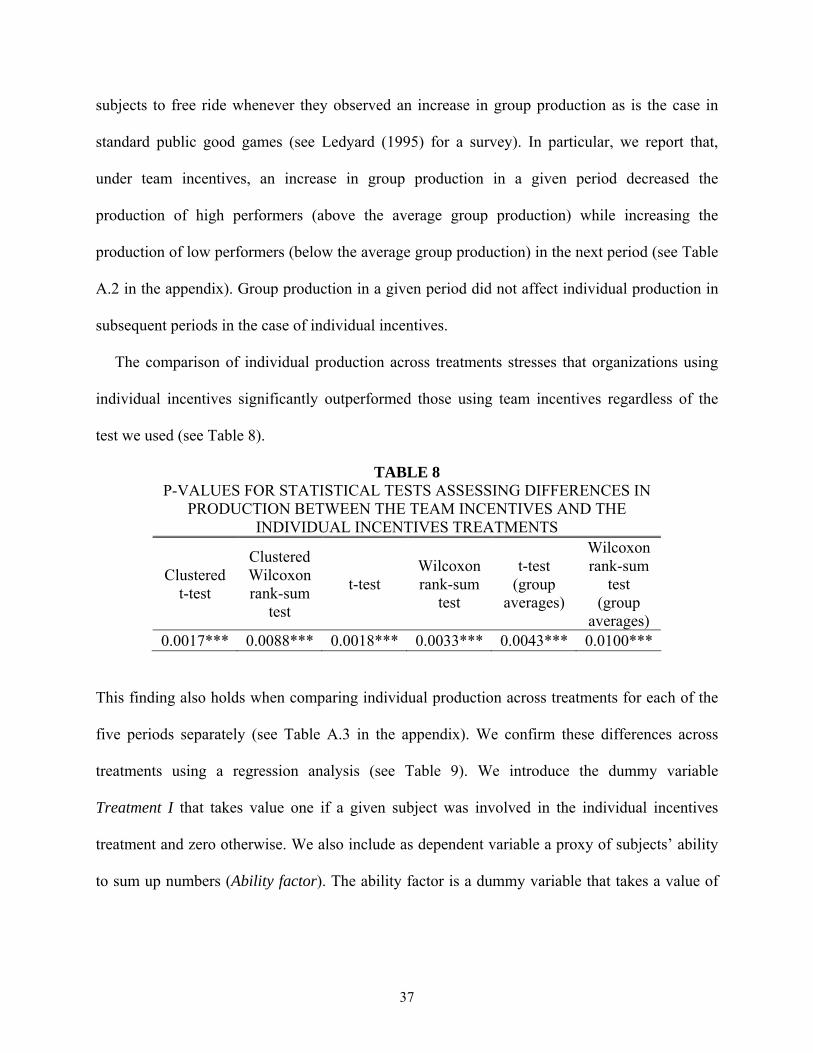
The comparison of individual production across treatments stresses that organizations using

individual incentives significantly outperformed those using team incentives regardless of the

test we used (see Table 8).

TABLE 8 P-VALUES FOR STATISTICAL TESTS ASSESSING DIFFERENCES IN

PRODUCTION BETWEEN THE TEAM INCENTIVES AND THE INDIVIDUAL INCENTIVES TREATMENTS

Clustered t-test

Clustered Wilcoxon rank-sum

test

t-test Wilcoxon rank-sum

test

t-test (group

averages)

Wilcoxon rank-sum

test (group

averages) 0.0017*** 0.0088*** 0.0018*** 0.0033*** 0.0043*** 0.0100***

This finding also holds when comparing individual production across treatments for each of the

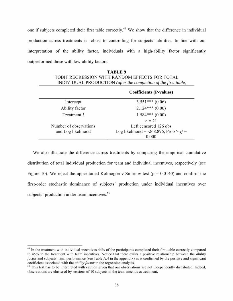
five periods separately (see Table A.3 in the appendix). We confirm these differences across

treatments using a regression analysis (see Table 9). We introduce the dummy variable

Treatment I that takes value one if a given subject was involved in the individual incentives

treatment and zero otherwise. We also include as dependent variable a proxy of subjects’ ability

to sum up numbers (Ability factor). The ability factor is a dummy variable that takes a value of

38

one if subjects completed their first table correctly.49 We show that the difference in individual

production across treatments is robust to controlling for subjects’ abilities. In line with our

interpretation of the ability factor, individuals with a high-ability factor significantly

outperformed those with low-ability factors.

TABLE 9 TOBIT REGRESSION WITH RANDOM EFFECTS FOR TOTAL

INDIVIDUAL PRODUCTION (after the completion of the first table)

Coefficients (P-values)

Intercept 3.551*** (0.06) Ability factor 2.124*** (0.00) Treatment I 1.584*** (0.00)




We also illustrate the difference across treatments by comparing the empirical cumulative

distribution of total individual production for team and individual incentives, respectively (see

Figure 10). We reject the upper-tailed Kolmogorov-Smirnov test (p = 0.0140) and confirm the

first-order stochastic dominance of subjects’ production under individual incentives over

subjects’ production under team incentives.50

49 In the treatment with individual incentives 44% of the participants completed their first table correctly compared to 45% in the treatment with team incentives. Notice that there exists a positive relationship between the ability factor and subjects’ final performance (see Table A.4 in the appendix) as is confirmed by the positive and significant coefficient associated with the ability factor in the regression analysis. 50 This test has to be interpreted with caution given that our observations are not independently distributed. Indeed, observations are clustered by sessions of 10 subjects in the team incentives treatment.

39

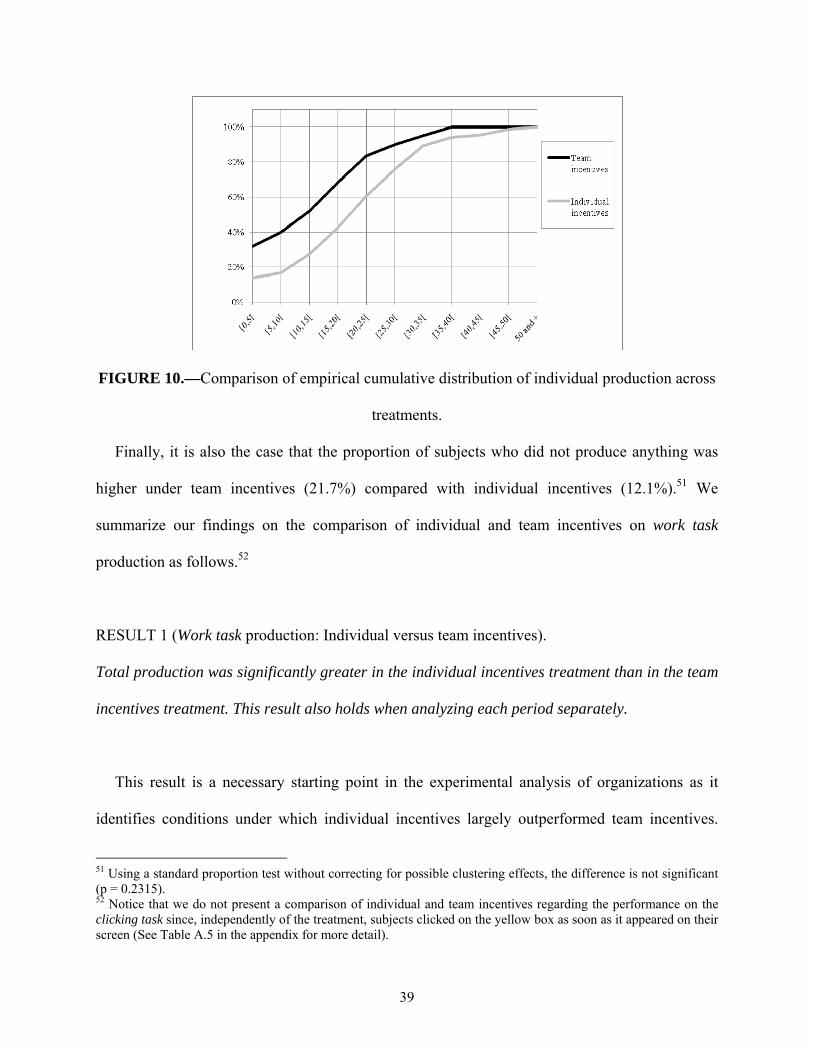
FIGURE 10.—Comparison of empirical cumulative distribution of individual production across

treatments.

Finally, it is also the case that the proportion of subjects who did not produce anything was

higher under team incentives (21.7%) compared with individual incentives (12.1%).51 We

summarize our findings on the comparison of individual and team incentives on work task

production as follows.52

RESULT 1 (Work task production: Individual versus team incentives).

Total production was significantly greater in the individual incentives treatment than in the team

incentives treatment. This result also holds when analyzing each period separately.

This result is a necessary starting point in the experimental analysis of organizations as it

identifies conditions under which individual incentives largely outperformed team incentives.

51 Using a standard proportion test without correcting for possible clustering effects, the difference is not significant (p = 0.2315). 52 Notice that we do not present a comparison of individual and team incentives regarding the performance on the clicking task since, independently of the treatment, subjects clicked on the yellow box as soon as it appeared on their screen (See Table A.5 in the appendix for more detail).

40

Organizations using individual incentives produced 52% more on average than those using

individual incentives. To our knowledge, this is the first time this result is established in a

controlled environment. This result is not surprising in the light of incentive theory (Hypothesis

1) but constitutes an essential step in the empirical analysis of incentives given the limited

evidence of free riding behaviors in teams (Dohmen and Falk (2011), Dumaine (1990, 1994),

Hamilton, Nickerson and Owan (2003), Hansen (1997), Ichniowski et al. (1996), Ichniowski,

Shaw and Prennushi (1997), Kruse (1992), Manz and Sims (1993), van Dijk, Sonnemans and van

Winden (2001)). Result 1 suggests that our experimental environment is well suited in order to

identify incentives effects and could prove to be a privileged platform for an empirical

assessment of the theory of incentives.

Given the negative effect of Internet usage on individual production identified in the case of

individual incentives, we expect the difference in individual production across treatments to be

reflected in the use of Internet. The comparison of Internet usage across treatments is analyzed in

more detail in the next section.

3.2.2. Internet Usage Comparison

We illustrate the sharp differences in Internet usage under individual and team incentives in

Figure 11. Under team incentives subjects spent 28.5% of their time on average to browse the

Internet while this percentage was only equal to 15.4% under individual incentives. Under team

incentives, subjects dedicated an average of 19.1% of their time to Internet activities in the first

two periods compared with 34.8% in the last three periods. The proportion of their time subjects

dedicated to Internet usage under team incentives (28.5%) was remarkably similar to the figures

published in the 2005 study by American Online and Salary.com according to which employees

41

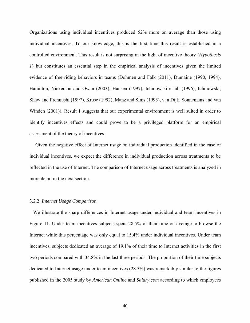
spend about 26.1% of their time on activities unrelated to their work (Malachowski (2005)).53,54

Notice that in our environment, Internet usage was the only leisure activity available to workers.

FIGURE 11.—Average time (in %) spent by subjects browsing the internet for individual and

team incentives treatments.

Similarly to the treatment with individual incentives, we find a positive trend in Internet usage

(see Table A.6 in the appendix).55 Internet usage increased significantly from Period 2

onwards.56 Similarly to the case of individual incentives, we find a sharp increase in Internet

usage in the last five minutes of each period during which subjects spent 39% of their time on the

web compared with 25% on average during the first fifteen minutes.57

We reject the hypothesis that Internet usage was identical for individual and team incentives

(see Table A.7 in the appendix). Under team incentives, Internet usage was about twice higher 53 Almost half of this time corresponds to Internet browsing. 54 In addition, 85% of the subjects in the team incentives treatment decided to browse the Internet during the experiment. This figure is close to the 2005 study by Web@Work that reports that 93% of the workers admit to visit Internet web pages during their work day. 55 Similarly to the case of individual incentives, we report a negative correlation between Internet usage and individual production since Pearson (Spearman) [Kendall] coefficients are equal to -0.6580 (-0.4754) [-0.6721] with p < 0.0001 in each case. 56 Under individual incentives, the increase in Internet usage occurred one period later as the period dummies were significant from Period 3 onwards (see Table 6). 57 The p-value for the Wilcoxon signed-rank test is inferior to 0.0001.

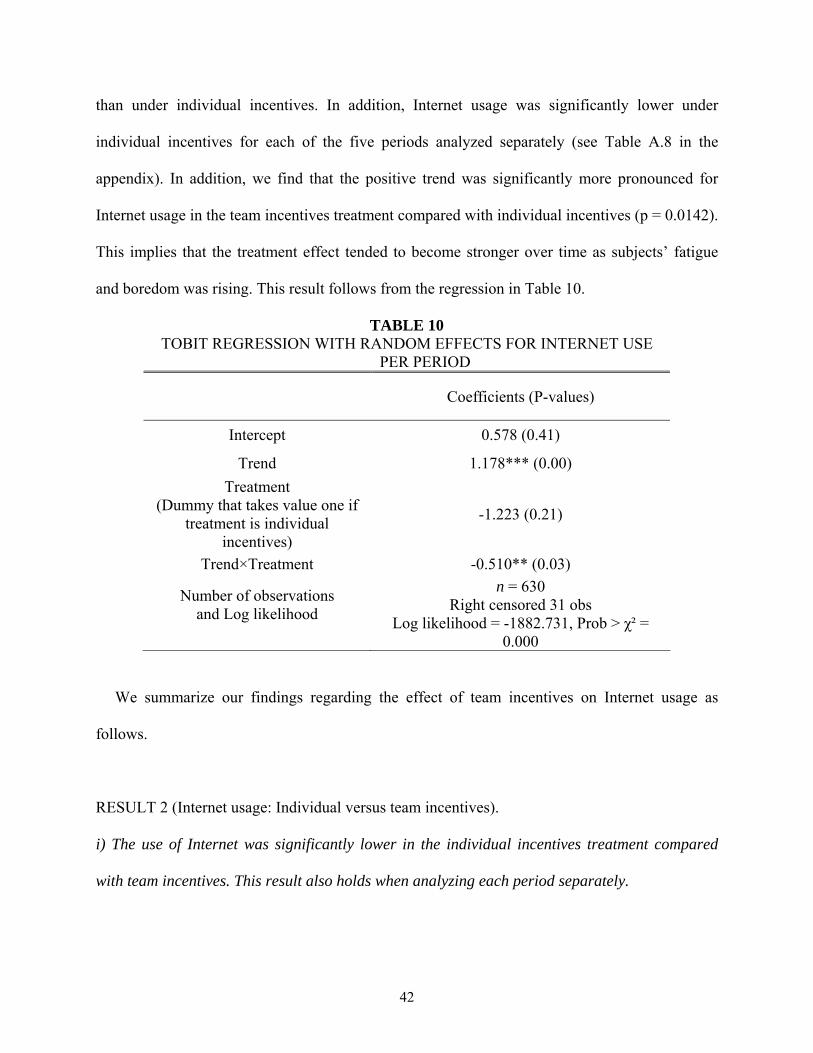
42

than under individual incentives. In addition, Internet usage was significantly lower under

individual incentives for each of the five periods analyzed separately (see Table A.8 in the

appendix). In addition, we find that the positive trend was significantly more pronounced for

Internet usage in the team incentives treatment compared with individual incentives (p = 0.0142).

This implies that the treatment effect tended to become stronger over time as subjects’ fatigue

and boredom was rising. This result follows from the regression in Table 10.

TABLE 10 TOBIT REGRESSION WITH RANDOM EFFECTS FOR INTERNET USE

PER PERIOD


Intercept 0.578 (0.41)

Trend 1.178*** (0.00) Treatment

(Dummy that takes value one if treatment is individual

incentives)

-1.223 (0.21)

Trend×Treatment -0.510** (0.03)




We summarize our findings regarding the effect of team incentives on Internet usage as

follows.

RESULT 2 (Internet usage: Individual versus team incentives).

i) The use of Internet was significantly lower in the individual incentives treatment compared

with team incentives. This result also holds when analyzing each period separately.

43

ii) The increase in Internet usage over time was significantly more pronounced in the team

incentives treatment than in the individual incentives treatment.

This finding emphasizes that, in an environment with a long and real-effort task in which

fatigue was likely to arise, high-powered incentives were very effective in bringing down

Internet usage. Indeed, subjects spent almost twice as long on Internet under team incentives than

under individual incentives. In sum, shirking behaviors prevailed in the presence of low-powered

incentives schemes.

This result is fundamental as it shows that increasing the level of realism in the experimental

environment leads to results that are consistent with incentives theory (see Holmström (1979),

and Laffont and Martimort (2002) for a review).

As a final step of our analysis, we introduce peer pressure in the virtual organization in order

to assess whether the performance of organizations using team incentives can be enhanced by the

use of real-time peer monitoring.

3.3. Peer Pressure

We start the analysis of peer monitoring by providing general statistics on watching activities.

The analysis of production levels and Internet usage is completed in Sections 3.3.2 and 3.3.3,

respectively.

3.3.1. Watching Activities

Subjects dedicated an average of 4.4% of their time to watching activities. They monitored

others 5.7 times during the experiment for an average duration of 46 seconds per watching

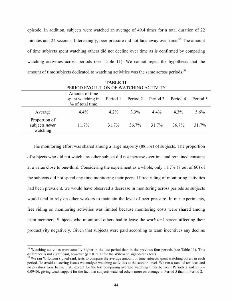
44

episode. In addition, subjects were watched an average of 49.4 times for a total duration of 22

minutes and 24 seconds. Interestingly, peer pressure did not fade away over time.58 The amount

of time subjects spent watching others did not decline over time as is confirmed by comparing

watching activities across periods (see Table 11). We cannot reject the hypothesis that the

amount of time subjects dedicated to watching activities was the same across periods.59

TABLE 11 PERIOD EVOLUTION OF WATCHING ACTIVITY

Amount of time

spent watching in % of total time

Period 1 Period 2 Period 3 Period 4 Period 5

Average 4.4% 4.2% 3.3% 4.4% 4.3% 5.6%

Proportion of subjects never

watching 11.7% 31.7% 36.7% 31.7% 36.7% 31.7%

The monitoring effort was shared among a large majority (88.3%) of subjects. The proportion

of subjects who did not watch any other subject did not increase overtime and remained constant

at a value close to one-third. Considering the experiment as a whole, only 11.7% (7 out of 60) of

the subjects did not spend any time monitoring their peers. If free riding of monitoring activities

had been prevalent, we would have observed a decrease in monitoring across periods as subjects

would tend to rely on other workers to maintain the level of peer pressure. In our experiments,

free riding on monitoring activities was limited because monitoring costs were shared among

team members. Subjects who monitored others had to leave the work task screen affecting their

productivity negatively. Given that subjects were paid according to team incentives any decline

58 Watching activities were actually higher in the last period than in the previous four periods (see Table 11). This difference is not significant, however (p = 0.7100 for the Wilcoxon signed-rank test). 59 We ran Wilcoxon signed-rank tests to compare the average amount of time subjects spent watching others in each period. To avoid clustering issues we analyze watching activities at the session level. We ran a total of ten tests and no p-values were below 0.20, except for the test comparing average watching times between Periods 2 and 5 (p = 0.0940), giving weak support for the fact that subjects watched others more on average in Period 5 than in Period 2.

45

in production due to monitoring activities would affect all workers in the same magnitude. Our

environment differs from the model presented by Alchian and Demsetz (1972) in which subjects

who are paid according to their individual contribution would incur an individual cost for

undertaking monitoring activities. Public good games with punishments also consider the case in

which the cost for sanctioning other subjects is fully incurred by the individual punisher (Fehr

and Gächter (2000)).

Interestingly, it was unlikely for subjects to watch the same person at the same time. This

occurred only in 16.7% of the watching episodes. It is then not surprising to report that all

subjects were watched during the experiment for a minimum duration as high as 12 minutes (that

is, 12% of the experiment time). In addition, the average proportion of subjects that were being

watched in a given minute was equal to 44.8%, while subjects’ dedication to monitoring

activities was limited to 4.4% of their time. This occurred because most watchers (94.2%)

decided to monitor all subjects at the same time. As a result, the amount of time subjects were

being watched during the experiment was similar across subjects.60 In particular, subjects with

different levels of performance were being watched for the same amount of time. It was not the

case that either low- or high- performers were more likely to be watched by others. We test this

conjecture by means of a regression analysis in which we introduce as dependent variables the

amount of time subjects were watching others as well as the amount of time they were being

watched by others (see Table A.9 in the appendix).61

Finally, it is interesting to note that subjects were as likely to be watched at the beginning, in

the middle or at the end of each period (see Figure 12). More precisely, we analyze whether the

60 In our experimental design, subjects could watch the other nine subjects at the same time by clicking on the monitor all button. In a related study (in progress), we focused on the specificities of the watching mechanism, we restrict the monitoring technology so that subjects can only watch a subset of coworkers at the same time. 61 We use a 5-minute time frame to assess the impact of past performance on watching others or being watched by others. The relationship between watching activities and subjects’ performance ranks is provided in Section 3.4

46

pattern of watching activities within a period followed a random pattern by using a random order

test.62 To that end, we define an indicator variable that takes value one if a subject has been

watching others in a given minute of a given period and takes value zero otherwise. Then, we

analyze for each period of each of the six sessions (that is a total of 30 observations) whether the

order of watching times followed a random order. We find that 25 out of 30 periods are

characterized by random watching times. Therefore, we conclude that the pattern of watching

times tended to follow a random order.We summarize our findings regarding watching activities

as follows.

RESULT 3 (Watching activities)

i) Watching activities were limited to a small percentage (4.4%) of subjects’ available time.

Nevertheless, all subjects were being watched during the experiment for an average of 22

minutes and 24 seconds (that is, 22.4% of the duration of the experiment).

ii) Watching activities did not fade away across periods.

iii) The pattern of watching activities followed a random order.

These results suggest that subjects were willing to exert peer pressure on others at any point

during the experiment. If subjects had only been interested in feedback about their relative

performance they may have used very short watching episodes concentrated toward the end of

each period. Following this strategy, subjects could have gathered all the information necessary

to assess their relative performance in a short amount of time. Instead, we find that subjects were

being watched extensively during the whole experiment.

62 We use the random order test in STATA and we consider that the pattern of watching in a given period is not random whenever the test rejects the null hypothesis at a 5% significance level (Swed and Eisenhart (1943)).

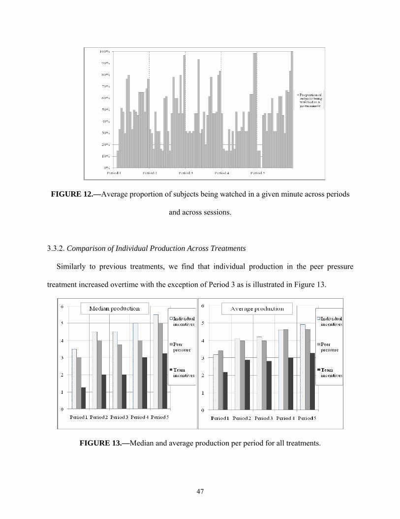
47

FIGURE 12.—Average proportion of subjects being watched in a given minute across periods

and across sessions.

3.3.2. Comparison of Individual Production Across Treatments

Similarly to previous treatments, we find that individual production in the peer pressure

treatment increased overtime with the exception of Period 3 as is illustrated in Figure 13.

FIGURE 13.—Median and average production per period for all treatments.

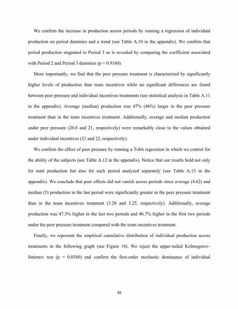
48

We confirm the increase in production across periods by running a regression of individual

production on period dummies and a trend (see Table A.10 in the appendix). We confirm that

period production stagnated in Period 3 as is revealed by comparing the coefficient associated

with Period 2 and Period 3 dummies (p = 0.9160).

More importantly, we find that the peer pressure treatment is characterized by significantly

higher levels of production than team incentives while no significant differences are found

between peer pressure and individual incentives treatments (see statistical analysis in Table A.11

in the appendix). Average (median) production was 47% (46%) larger in the peer pressure

treatment than in the team incentives treatment. Additionally, average and median production

under peer pressure (20.6 and 21, respectively) were remarkably close to the values obtained

under individual incentives (21 and 22, respectively).

We confirm the effect of peer pressure by running a Tobit regression in which we control for

the ability of the subjects (see Table A.12 in the appendix). Notice that our results hold not only

for total production but also for each period analyzed separately (see Table A.13 in the

appendix). We conclude that peer effects did not vanish across periods since average (4.62) and

median (5) production in the last period were significantly greater in the peer pressure treatment

than in the team incentives treatment (3.28 and 3.25, respectively). Additionally, average

production was 47.3% higher in the last two periods and 46.7% higher in the first two periods

under the peer pressure treatment compared with the team incentives treatment.

Finally, we represent the empirical cumulative distribution of individual production across

treatments in the following graph (see Figure 14). We reject the upper-tailed Kolmogorov-

Smirnov test (p = 0.0380) and confirm the first-order stochastic dominance of individual

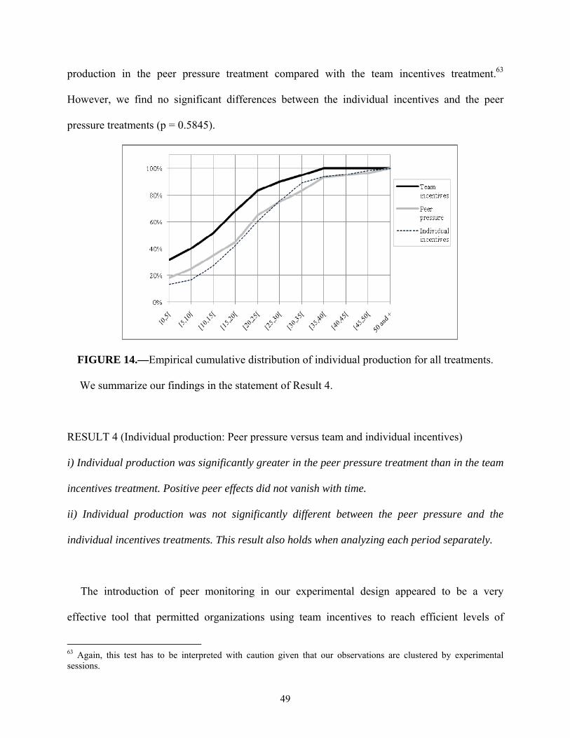
49

production in the peer pressure treatment compared with the team incentives treatment.63

However, we find no significant differences between the individual incentives and the peer

pressure treatments (p = 0.5845).

FIGURE 14.—Empirical cumulative distribution of individual production for all treatments.

We summarize our findings in the statement of Result 4.

RESULT 4 (Individual production: Peer pressure versus team and individual incentives)

i) Individual production was significantly greater in the peer pressure treatment than in the team

incentives treatment. Positive peer effects did not vanish with time.

ii) Individual production was not significantly different between the peer pressure and the

individual incentives treatments. This result also holds when analyzing each period separately.

The introduction of peer monitoring in our experimental design appeared to be a very

effective tool that permitted organizations using team incentives to reach efficient levels of

63 Again, this test has to be interpreted with caution given that our observations are clustered by experimental sessions.

50

production.64 This result is practically relevant for managers who usually possess limited

information about individual contributions, and as a result, cannot rely on individual incentives

schemes.

To our knowledge, this is the first time this result is established empirically. Evidence of

positive peer effects has been identified in field studies (Falk and Ichino (2006), Mas and Moretti

(2009)), but none of these works have examined peer monitoring as a mechanism to resolve free

riding in teams. It is also interesting to observe that we obtained strong peer monitoring effects in

the absence of punishment devices or threats. It is indeed well known that punishments can be

very effective in increasing contributions in public good games (Fehr and Gächter (2000),

Masclet et al. (2003), Sefton, Shupp and Walker (2007)). Notice that in field studies such as the

one designed by Mas and Moretti (2009), workers were not anonymous and could potentially

face retaliation for non-cooperative behaviors. In our design, subjects were anonymous and this

prevented any form of retaliation after the experiment. In contrast to field studies (Falk and

Ichino (2006), Mas and Moretti (2009)) and public good games with threats (Masclet et al.

(2003)), subjects were not allowed to communicate in our experiment. Finally, our peer

monitoring technology did not rely on physical proximity and face to face interactions. Instead,

subjects remained seated at their workstation while monitoring others. Supervisees simply

received a notification on their screen that they were currently being watched by another subject.

The fact that our monitoring technology was highly effective despite the absence of physical

proximity and face to face communication is especially relevant given the growing interest for

virtual monitoring devices within firms.65

64 We interpret the level of production obtained under individual incentives as the efficient level. 65 A large number of programs such as Spectorsoft, Virtual Monitoring™, Employee Monitoring or Webwatcher are already available to monitor employees’ activities. An early account of computer-based monitoring systems was considered in Chalykoff and Kochan (1989).

51

Our result is related to the audience effects documented in the literature in social facilitation,

starting with the seminal works of Zajonc (1965, 1980). The author puts forward that a subject’s

performance on a given task is likely to be affected by the presence of others. In particular,

Zajonc stresses that the presence of others affects performance positively for simple and well-

learnt tasks while affecting performance negatively for more complex tasks. Our result regarding

the positive effect or peer pressure on individual production is consistent with Zajonc’s social

facilitation theory if we consider summing numbers as a well-learnt task for a pool of

undergraduate students. This finding is particularly striking if we take into account that monitors

were not physically present at supervisees’ workstations in contrast with the context envisioned

by Zajonc in his theory of audience effects. Our findings suggest that the presence effects

highlighted by Zajonc are robust to the case of virtual monitoring.

Despite the fact that our monitoring mechanism involves no physical proximity and no face to

face interaction it constitutes a stronger mechanism than devices that simply rely on cues of

being watched without implementing real supervision. Recent studies show that cues of being

watched such as the display of the picture of eyes on the subject’s screen (Bateson, Nettle and

Roberts (2006)) tends to increase cooperative behaviors in a context in which students were

collecting money for drinks. Relatedly, Burnham and Hare (2007) find evidence of increased

cooperation in a public good game experiment in which the picture of a robot’s face with

prominent eyes was displayed on the screen. These findings suggest that not only being watched

by others but cues of being watched may increase cooperative behavior. In our experimental

design, we did not use cues as subjects knew that the eye picture only appeared when other

subjects were currently watching them. Subjects who were being watched by others were

52

informed about the experiment ID of the watchers so as to eliminate speculations regarding the

possible attempt of the experimenter to use deceptive strategies.

Our result can also be interpreted in the light of audience effects reported by economists who

stress that people may like to be perceived by others as altruistic and fair (Andreoni and

Bernheim (2009), Levine (1998)). In our environment, subjects may have been willing to signal

themselves as hard-working and cooperative to the person that was watching them. Relatedly,

the power of peer pressure as was initially described by Kandel and Lazear (1992) is linked to

the power of shame (Tadelis (2011)) by which workers may feel uncomfortable contributing less

than the group average and decide to work harder as a result. The positive effect of peer

monitoring is also consistent with early research in Sociology stressing that group incentives lead

to low levels of shirking. Indeed, members of a work group tend to feel as if they shared a

common fate, responding to peer pressure by increasing their contribution to the group because

of the fear of disapproval from other members (Homans (1951), Roy (1953), Whyte (1955)).66

Result 4 is also in line with empirical evidence suggesting that mutual monitoring in work

groups has been a decisive factor in the success of low-powered firm-wide incentives schemes as

is described in the case of Continental Airlines (Knez and Simester (2001)). The authors mention

shame as well as sanctioning as possible mechanisms inducing positive peer pressure. In this

paper, we shed light on the relevance of peer pressure effects in a controlled environment in

which subjects could not sanction their partners monetarily nor threat them verbally.

Furthermore, we investigate the impact of watching episodes on individual production during

the experiment. We perform a regression analysis in which we use as independent variables the

amount of time subjects spent watching others as well as the amount of time subjects were being

watched by others. This regression analysis allows us to disentangle the effect of watching others 66 This position has been later criticized (e.g. Orr (2001)).

53

from the effect of being watched by others. In addition, we are able to study the dynamic

structure of the effect of watching activities on individual production.

In our analysis, we use a 5-minute time frame so as to assess the impact of watching activities

on real-time production.67 The independent variables related to watching activities are referred to

as Watching and Being watched. These variables measure the amount of time (in seconds) that a

subject spent watching others (Watching) and the amount of time (in seconds) a subject was

watched (Being watched) by at least one subject in a given time span of five minutes. We

introduce independent variables with lags so as to mitigate possible endogeneity issues.68 We

include a trend as independent variable so as to control for the steady increase of production

across periods.69 Finally, we control for subjects’ ability by adding the ability factor as

independent variable. We provide the estimates for the regression analysis in Table 12.70We

conclude from our regression analysis that being watched by others affected individual

production positively in the next five to ten minutes. The delay in the impact of watching

activities can be accounted for the time subjects needed to produce a table (4 minutes and 3

seconds on average) and increase individual production as a result. Furthermore, subjects who

responded positively to peer monitoring by switching from the Internet screen to the work task

67 Notice that an analysis with shorter time intervals (e.g. intervals of one minute) may not be adequate since subjects need on average 4 minutes and 3 seconds to complete a table. 68 Endogeneity issues may arise if we introduce the current amount of time subjects spent watching others as well as the current amount of time they were being watched by others as independent variables. Indeed, one may expect that individual production could cause changes in watching behaviors. For example, subjects with low levels of production may feel ashamed (Kandel and Lazear (1992)) and decide to avoid consulting the performance of others. 69 Similar results are obtained when controlling for beginning or end of period effects. For example, the nature of our results is unchanged when introducing in our regression analysis a dummy variable that takes value one if the five minute time span corresponds to the first (last) five minutes of the period. 70 A number of other specifications have been considered such as including up to three lags in the independent variables or adding group production in the previous period as regressors. These specifications gave similar results. We also used dynamic panel data models with Arellano-Bond (1991) estimation technique. However, this estimation technique was not successful in fully eliminating residual autocorrelation as we may expect given the limited number of instrumental variables at our disposal.

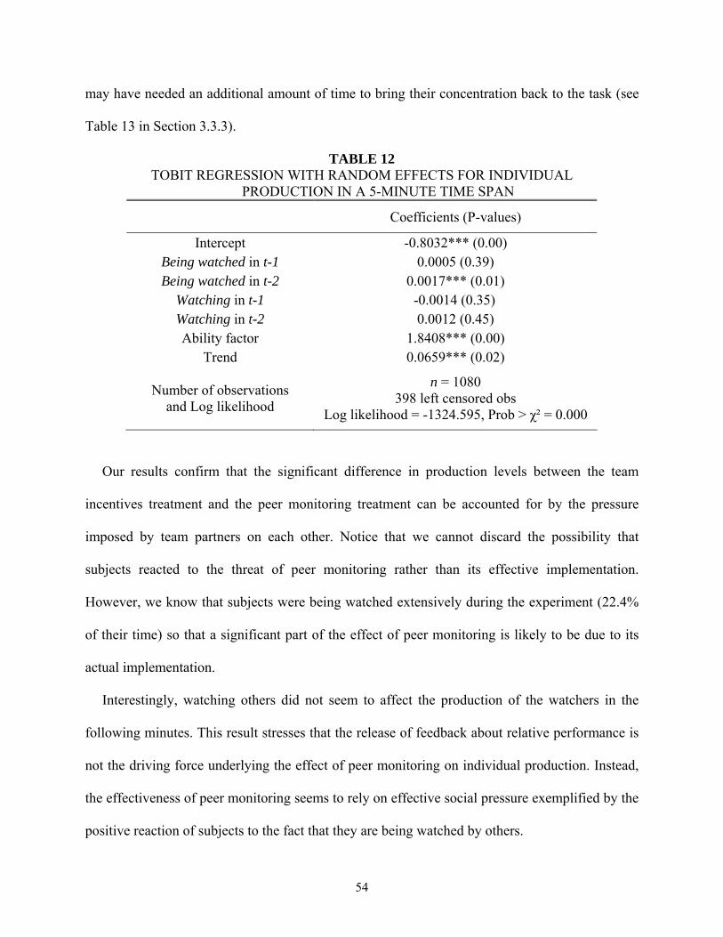
54

may have needed an additional amount of time to bring their concentration back to the task (see

Table 13 in Section 3.3.3).

TABLE 12 TOBIT REGRESSION WITH RANDOM EFFECTS FOR INDIVIDUAL

PRODUCTION IN A 5-MINUTE TIME SPAN


Intercept -0.8032*** (0.00) Being watched in t-1 0.0005 (0.39) Being watched in t-2 0.0017*** (0.01)

Watching in t-1 -0.0014 (0.35) Watching in t-2 0.0012 (0.45) Ability factor 1.8408*** (0.00)

Trend 0.0659*** (0.02)


n = 1080 398 left censored obs


Our results confirm that the significant difference in production levels between the team

incentives treatment and the peer monitoring treatment can be accounted for by the pressure

imposed by team partners on each other. Notice that we cannot discard the possibility that

subjects reacted to the threat of peer monitoring rather than its effective implementation.

However, we know that subjects were being watched extensively during the experiment (22.4%

of their time) so that a significant part of the effect of peer monitoring is likely to be due to its

actual implementation.

Interestingly, watching others did not seem to affect the production of the watchers in the

following minutes. This result stresses that the release of feedback about relative performance is

not the driving force underlying the effect of peer monitoring on individual production. Instead,

the effectiveness of peer monitoring seems to rely on effective social pressure exemplified by the

positive reaction of subjects to the fact that they are being watched by others.

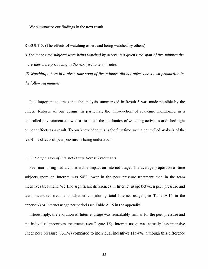
55

We summarize our findings in the next result.

RESULT 5. (The effects of watching others and being watched by others)

i) The more time subjects were being watched by others in a given time span of five minutes the

more they were producing in the next five to ten minutes.

ii) Watching others in a given time span of five minutes did not affect one’s own production in

the following minutes.

It is important to stress that the analysis summarized in Result 5 was made possible by the

unique features of our design. In particular, the introduction of real-time monitoring in a

controlled environment allowed us to detail the mechanics of watching activities and shed light

on peer effects as a result. To our knowledge this is the first time such a controlled analysis of the

real-time effects of peer pressure is being undertaken.

3.3.3. Comparison of Internet Usage Across Treatments

Peer monitoring had a considerable impact on Internet usage. The average proportion of time

subjects spent on Internet was 54% lower in the peer pressure treatment than in the team

incentives treatment. We find significant differences in Internet usage between peer pressure and

team incentives treatments whether considering total Internet usage (see Table A.14 in the

appendix) or Internet usage per period (see Table A.15 in the appendix).

Interestingly, the evolution of Internet usage was remarkably similar for the peer pressure and

the individual incentives treatments (see Figure 15). Internet usage was actually less intensive

under peer pressure (13.1%) compared to individual incentives (15.4%) although this difference

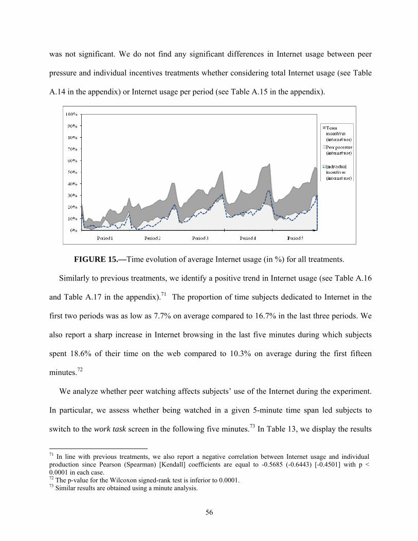
56

was not significant. We do not find any significant differences in Internet usage between peer

pressure and individual incentives treatments whether considering total Internet usage (see Table

A.14 in the appendix) or Internet usage per period (see Table A.15 in the appendix).

FIGURE 15.—Time evolution of average Internet usage (in %) for all treatments.

Similarly to previous treatments, we identify a positive trend in Internet usage (see Table A.16

and Table A.17 in the appendix).71 The proportion of time subjects dedicated to Internet in the

first two periods was as low as 7.7% on average compared to 16.7% in the last three periods. We

also report a sharp increase in Internet browsing in the last five minutes during which subjects

spent 18.6% of their time on the web compared to 10.3% on average during the first fifteen

minutes.72

We analyze whether peer watching affects subjects’ use of the Internet during the experiment.

In particular, we assess whether being watched in a given 5-minute time span led subjects to

switch to the work task screen in the following five minutes.73 In Table 13, we display the results

71 In line with previous treatments, we also report a negative correlation between Internet usage and individual production since Pearson (Spearman) [Kendall] coefficients are equal to -0.5685 (-0.6443) [-0.4501] with p < 0.0001 in each case. 72 The p-value for the Wilcoxon signed-rank test is inferior to 0.0001. 73 Similar results are obtained using a minute analysis.

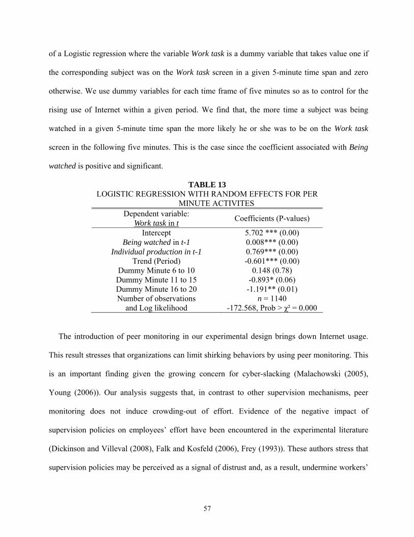
57

of a Logistic regression where the variable Work task is a dummy variable that takes value one if

the corresponding subject was on the Work task screen in a given 5-minute time span and zero

otherwise. We use dummy variables for each time frame of five minutes so as to control for the

rising use of Internet within a given period. We find that, the more time a subject was being

watched in a given 5-minute time span the more likely he or she was to be on the Work task

screen in the following five minutes. This is the case since the coefficient associated with Being

watched is positive and significant.

TABLE 13 LOGISTIC REGRESSION WITH RANDOM EFFECTS FOR PER

MINUTE ACTIVITES Dependent variable:

Work task in t Coefficients (P-values)

Intercept 5.702 *** (0.00) Being watched in t-1 0.008*** (0.00)

Individual production in t-1 0.769*** (0.00) Trend (Period) -0.601*** (0.00)

Dummy Minute 6 to 10 0.148 (0.78) Dummy Minute 11 to 15 -0.893* (0.06) Dummy Minute 16 to 20 -1.191** (0.01) Number of observations

and Log likelihood n = 1140

-172.568, Prob > χ² = 0.000

The introduction of peer monitoring in our experimental design brings down Internet usage.

This result stresses that organizations can limit shirking behaviors by using peer monitoring. This

is an important finding given the growing concern for cyber-slacking (Malachowski (2005),

Young (2006)). Our analysis suggests that, in contrast to other supervision mechanisms, peer

monitoring does not induce crowding-out of effort. Evidence of the negative impact of

supervision policies on employees’ effort have been encountered in the experimental literature

(Dickinson and Villeval (2008), Falk and Kosfeld (2006), Frey (1993)). These authors stress that

supervision policies may be perceived as a signal of distrust and, as a result, undermine workers’

58

effort. Frey (1993) as well as Dickinson and Villeval (2008) put forward that the crowding-out

effect that results from monitoring activities dominates its disciplining effect when there exist

interpersonal relationships between managers and employees whereas the opposite tends to be

true in the absence of such relationships. In that respect, our findings are consistent with the

works of Frey (1993) and Dickinson and Villeval (2008) since our experimental design is

characterized by the absence of interpersonal relationships among workers.

Furthermore, we believe that crowding-out effects are likely to be stronger in a principal-agent

relationship or in any organizational structure in which the monitor has some authority over the

supervisee’s work. By contrast, our design is characterized by a multi-agent monitoring structure

in which there is no principal and no hierarchy since each subject has the same role. In that

context, we show that the disciplining effect of peer monitoring dominates the crowding-out

effect.

We summarize our findings as follows.

RESULT 6 (Internet usage: Peer pressure versus team and individual incentives)

i) The use of Internet was significantly lower in the peer pressure treatment than in the team

incentives treatment. Internet usage was not significantly different between the peer pressure and

the individual incentives treatments.

ii) Subjects were more likely to switch from Internet to the work task if they had been watched by

others in the previous minute.

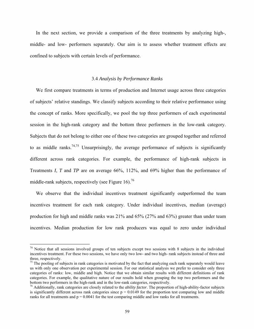
59

In the next section, we provide a comparison of the three treatments by analyzing high-,

middle- and low- performers separately. Our aim is to assess whether treatment effects are

confined to subjects with certain levels of performance.

3.4 Analysis by Performance Ranks

We first compare treatments in terms of production and Internet usage across three categories

of subjects’ relative standings. We classify subjects according to their relative performance using

the concept of ranks. More specifically, we pool the top three performers of each experimental

session in the high-rank category and the bottom three performers in the low-rank category.

Subjects that do not belong to either one of these two categories are grouped together and referred

to as middle ranks.74,75 Unsurprisingly, the average performance of subjects is significantly

different across rank categories. For example, the performance of high-rank subjects in

Treatments I, T and TP are on average 66%, 112%, and 69% higher than the performance of

middle-rank subjects, respectively (see Figure 16).76

We observe that the individual incentives treatment significantly outperformed the team

incentives treatment for each rank category. Under individual incentives, median (average)

production for high and middle ranks was 21% and 65% (27% and 63%) greater than under team

incentives. Median production for low rank producers was equal to zero under individual

74 Notice that all sessions involved groups of ten subjects except two sessions with 8 subjects in the individual incentives treatment. For these two sessions, we have only two low- and two high- rank subjects instead of three and three, respectively. 75 The pooling of subjects in rank categories is motivated by the fact that analyzing each rank separately would leave us with only one observation per experimental session. For our statistical analysis we prefer to consider only three categories of ranks: low, middle and high. Notice that we obtain similar results with different definitions of rank categories. For example, the qualitative nature of our results hold when grouping the top two performers and the bottom two performers in the high-rank and in the low-rank categories, respectively. 76 Additionally, rank categories are closely related to the ability factor. The proportion of high-ability-factor subjects is significantly different across rank categories since p = 0.0149 for the proportion test comparing low and middle ranks for all treatments and p = 0.0041 for the test comparing middle and low ranks for all treatments.

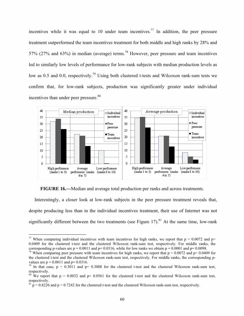
60

incentives while it was equal to 10 under team incentives.77 In addition, the peer pressure

treatment outperformed the team incentives treatment for both middle and high ranks by 28% and

57% (27% and 63%) in median (average) terms.78 However, peer pressure and team incentives

led to similarly low levels of performance for low-rank subjects with median production levels as

low as 0.5 and 0.0, respectively.79 Using both clustered t-tests and Wilcoxon rank-sum tests we

confirm that, for low-rank subjects, production was significantly greater under individual

incentives than under peer pressure.80

FIGURE 16.—Median and average total production per ranks and across treatments.

Interestingly, a closer look at low-rank subjects in the peer pressure treatment reveals that,

despite producing less than in the individual incentives treatment, their use of Internet was not

significantly different between the two treatments (see Figure 17).81 At the same time, low-rank

77 When comparing individual incentives with team incentives for high ranks, we report that p = 0.0072 and p= 0.0409 for the clustered t-test and the clustered Wilcoxon rank-sum test, respectively. For middle ranks, the corresponding p-values are p = 0.0011 and p= 0.0316, while for low ranks we obtain p = 0.0001 and p= 0.0098. 78 When comparing peer pressure with team incentives for high ranks, we report that p = 0.0072 and p= 0.0409 for the clustered t-test and the clustered Wilcoxon rank-sum test, respectively. For middle ranks, the corresponding p-values are p = 0.0011 and p= 0.0316. 79 In that case, p = 0.3011 and p= 0.3008 for the clustered t-test and the clustered Wilcoxon rank-sum test, respectively. 80 We report that p = 0.0032 and p= 0.0561 for the clustered t-test and the clustered Wilcoxon rank-sum test, respectively. 81 p = 0.8226 and p = 0.7242 for the clustered t-test and the clustered Wilcoxon rank-sum test, respectively.

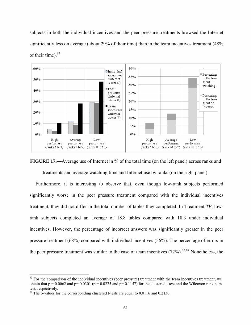
61

subjects in both the individual incentives and the peer pressure treatments browsed the Internet

significantly less on average (about 29% of their time) than in the team incentives treatment (48%

of their time).82

FIGURE 17.—Average use of Internet in % of the total time (on the left panel) across ranks and

treatments and average watching time and Internet use by ranks (on the right panel).

Furthermore, it is interesting to observe that, even though low-rank subjects performed

significantly worse in the peer pressure treatment compared with the individual incentives

treatment, they did not differ in the total number of tables they completed. In Treatment TP, low-

rank subjects completed an average of 18.8 tables compared with 18.3 under individual

incentives. However, the percentage of incorrect answers was significantly greater in the peer

pressure treatment (68%) compared with individual incentives (56%). The percentage of errors in

the peer pressure treatment was similar to the case of team incentives (72%).83,84 Nonetheless, the

82 For the comparison of the individual incentives (peer pressure) treatment with the team incentives treatment, we obtain that p = 0.0062 and p= 0.0301 (p = 0.0225 and p= 0.1157) for the clustered t-test and the Wilcoxon rank-sum test, respectively. 83 The p-values for the corresponding clustered t-tests are equal to 0.0116 and 0.2130.

62

total number of tables completed was significantly greater in the peer pressure treatment (18.8)

compared with the team incentives treatment (13.4).85 In summary, subjects who were involved in

the peer pressure treatment tried more on the work task than subjects who did not face peer

pressure, but their level of accuracy was not significantly increased.86 These findings are

consistent with Eriksson, Poulsen and Villeval (2009) who show that providing continuous

feedback about others’ performance to low performers decreased their level of accuracy in a

summation task similar to the one used in the current experiment.87

Notice that the poor performance of low-rank subjects in the peer pressure treatment is not

driven by differences in watching activities. Indeed, subjects were being monitored for the same

amount of time independently of their rank. In particular, high-rank subjects were being watched

for 22.3 minutes on average while middle-rank subjects and low-rank subjects were being

watched for 22.8 and 21.9 minutes, respectively.88 It is also the case that subjects belonging to

different rank categories do not differ regarding the average amount of time they spent watching

others. Low-, middle- and high- rank subjects spent on average 3.8, 3.7 and 5.8 minutes watching

others. These differences are not significant.89

84 It is also the case for each of the three treatments that high-rank (middle-rank) subjects are characterized by a significantly lower percentage of errors and a significantly greater number of total answers compared to middle-rank (low-rank) subjects. We do not report these results because of space constraints. 85 The p-value for the corresponding one-sided clustered t-test is equal to 0.0325. 86 Notice that a similar result is obtained if we pool subjects according to their ability factor instead of their rank category. For low-ability subjects, the percentage of incorrect answers under individual incentives is equal to 44.3% while it is equal to 56.2% and 60.9% for Treatments TP and T, respectively. 87 Bandiera, Larcinese and Rasul (2010) do not report any positive effect of individual feedback on students’ performance in the case of low performers. In a related study, Azmat and Iriberri (2010) identify positive effects of feedback on relative performance for the whole range of ability levels. Sacerdote (2001), Tran and Zeckhauser (2009) and Zimmerman (2003) also report positive peer effects. 88 These differences are not significant. We use clustered Wilcoxon rank-sum test and obtain p = 0.5360 when comparing low and middle ranks, and p = 0.3709 when comparing low and high ranks. The p-value for the comparison of middle and high ranks was equal to 0.5819. Similar results are obtained using clustered t-tests. 89 Notice that median watching times are equal to 3.8, 3.7 and 3.4, respectively. Using a clustered t-test (clustered Wilcoxon rank-sum test) we obtain p = 0.7586 (p = 0.2441) when comparing low and middle ranks while p = 0.1520 (p = 0.4758) when comparing low and high ranks, and p = 0.1860 (p = 0.6838) when comparing middle and high ranks.

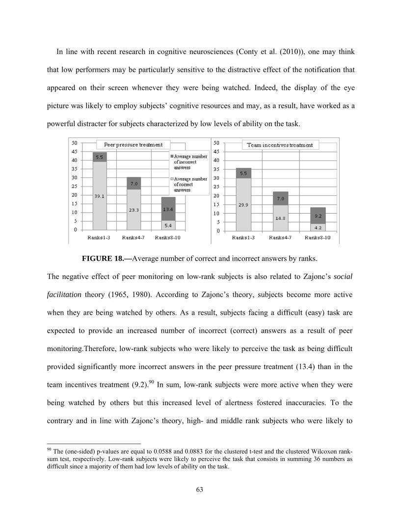
63

In line with recent research in cognitive neurosciences (Conty et al. (2010)), one may think

that low performers may be particularly sensitive to the distractive effect of the notification that

appeared on their screen whenever they were being watched. Indeed, the display of the eye

picture was likely to employ subjects’ cognitive resources and may, as a result, have worked as a

powerful distracter for subjects characterized by low levels of ability on the task.

FIGURE 18.—Average number of correct and incorrect answers by ranks.

The negative effect of peer monitoring on low-rank subjects is also related to Zajonc’s social

facilitation theory (1965, 1980). According to Zajonc’s theory, subjects become more active

when they are being watched by others. As a result, subjects facing a difficult (easy) task are

expected to provide an increased number of incorrect (correct) answers as a result of peer

monitoring.Therefore, low-rank subjects who were likely to perceive the task as being difficult

provided significantly more incorrect answers in the peer pressure treatment (13.4) than in the

team incentives treatment (9.2).90 In sum, low-rank subjects were more active when they were

being watched by others but this increased level of alertness fostered inaccuracies. To the

contrary and in line with Zajonc’s theory, high- and middle rank subjects who were likely to

90 The (one-sided) p-values are equal to 0.0588 and 0.0883 for the clustered t-test and the clustered Wilcoxon rank-sum test, respectively. Low-rank subjects were likely to perceive the task that consists in summing 36 numbers as difficult since a majority of them had low levels of ability on the task.

64

perceive the task as easy, completed more tables and achieved a greater level of accuracy in the

peer pressure treatment than in the team incentives treatment (see Figure 18).91

We confirm this interpretation of our findings by separately analyzing the impact of watching

activities on individual production for low-rank and middle to high rank subjects.92 We provide

the regression estimates in the appendix (Table A.18). In line with social facilitation theory, we

observe that being watched by others affected individual production negatively for subjects who

were low performers while the opposite was true for middle to high performers.

RESULT 7 (Peer pressure versus team incentives and individual incentives across ranks)

i) (High and Middle Rank: Production) Production was significantly greater in the peer pressure

treatment than in the team incentives treatment for high- and middle- ranks. We found no

differences in individual production between the peer pressure treatment and the individual

incentives treatment.

ii) (High and Middle Rank: Internet) Internet usage was significantly lower in the peer pressure

treatment than in the team incentives treatment for high- and middle- rank categories. We found

no differences in Internet usage between the peer pressure treatment and the individual


ii) (Low Rank: Production) Production was not significantly different in the peer pressure

treatment than in the team incentives treatment. However, production was significantly lower in

91 Comparing the number of tables completed across treatments, we obtain (one-sided) p-values equal to 0.0031 and 0.0198 for the clustered t-test and the clustered Wilcoxon rank-sum test, respectively. Comparing inaccuracy rates, we obtain (one-sided) p-values equal to 0.0439 and 0.0671 for the clustered t-test and the clustered Wilcoxon rank-sum test, respectively. 92 We completed this regression analysis in Section 3.3.2 (Table 12) for the whole sample of subjects.

65

the peer pressure treatment as well as in the team incentives treatment than in the individual


iii) (Low Rank: Internet) Internet usage was significantly lower in the peer pressure treatment

than in the team incentives treatment. However, we found no differences in Internet usage

between the peer pressure treatment and the individual incentives treatment.

v) The more time low-rank subjects were being watched by others in a given time span the less

they produced in the following minutes. The opposite was true for high- and middle- rank

subjects.

4. CONCLUSIONS

The primary objective of this research endeavor was to propose an empirical methodology for

the analysis of organizational issues in the laboratory. To that end, we incorporated several

crucial features of existing firms in a virtual organization. We allowed subjects to allocate their

time between a real-effort task that created value for the organization and a real-leisure activity.

We considered the most decentralized form of organizations in which no hierarchies existed and

all subjects had the same role. This represented a natural starting point that guided us in our quest

to identify the elements that lead to organizational success.

As a first step, we compared organizations using team and individual incentives in order to

assess the relevance of incentives effects in our virtual organizations. We found that individual

incentives led to levels of production that were 52% higher and levels of Internet usage that were

46% lower than under team incentives. These findings confirmed that implementing high-

powered incentives schemes is an important factor of organizational success consistently with

theoretical research (Holmström (1979), see Laffont and Martimort (2002) for a review).

66

Nevertheless, most organizations are limited in their use of individual incentives as a result of

asymmetric information (Alchian and Demsetz (1972), Holmström (1982)) and may have to

resort to alternative mechanisms to achieve high production levels.

We studied peer monitoring as an example of mechanism that may allow organizations to

recover the efficiency loss provoked by the use of team incentives. We found that using peer

monitoring in combination with team incentives allowed organizations to reach production levels

that were as high as in the case of individual incentives. The use of peer monitoring reduced

shirking behaviors. In particular, Internet usage was 54% lower for organizations relying on peer

monitoring compared with those using team incentives alone. In contrast to public good games

with punishments, both effort and efficiency were increased by the use of peer monitoring. To our

knowledge, ours is the first controlled experiment showing that peer monitoring can offset the

loss in efficiency resulting from the use of low-powered incentives schemes. Peer monitoring was

particularly effective because subjects spent a limited amount of time watching others (4.4% of

their time) while sharing the monitoring burden so that all subjects were being watched at least

once during the experiment. It is as if people possessed natural skills for peer monitoring and

understood both its positive effect on productivity as well as the negative consequences of its

intensive use. However, the positive impact of peer pressure on productivity did not apply to low

performers even though peer pressure pushed them to work harder and reduce their Internet

usage. The increase in effort did not translate into an increase in productivity as low performers

became less accurate as a result of peer monitoring.

In summary, peer-pressure was a very effective mechanism by which organizations using team

incentives achieved production levels that were remarkably close to those of organizations relying

on individual incentives schemes. This is good news for most organizations that cannot rely on

67

precise measures of individual contributions. Peer monitoring is traditionally seen as a decisive

advantage of organizations with respect to markets as its effectiveness usually relies on face to

face and repeated interactions among parties that are inherent to the organizational environment

(Bandiera, Barankay and Rasul (2005), Falk and Ichino (2006), Mas and Moretti (2009)).

However, the implementation of virtual monitoring devices of the type used in the present paper

may mitigate this comparative advantage of organizations as it may raise the effectiveness of peer

monitoring in the completion of market transactions.

68

5. REFERENCES

Aghion, P., and J. Tirole (1997): “Formal and Real Authority in Organizations,” Journal of Political Economy, 105, 1-29.

Alchian, A., and H. Demsetz (1972), “Production, information costs, and economic organization,” American Economic Review, 62, 777-795.

Alvero, A. M., B. R. Bucklin, and J. Austin (2001): “An objective review of the effectiveness and essential characteristics of performance feedback in organizational settings,” Journal of Organizational Behavior Management, 21(1), 3-29.

Andreoni, J., And B. D. Bernheim (2009): “Social Image and the 50–50 Norm: A Theoretical and Experimental Analysis of Audience Effects,” Econometrica, 77(5), 1607–1636.

Arellano, M., and S. Bond (1991): “Some tests of specification for panel data: Monte Carlo evidence and an application to employment equations,” The Review of Economic Studies, 58, 277–297.

Azmat, G., and N. Iriberri (2010): “The Importance of Relative Performance Feedback Information: Evidence from a Natural Experiment using High School Students,” Journal of Public Economics, 94(7-8), 435-452.

Balcazar, F., B.L. Hopkins, and Y. Suarez (1985–86): “A critical, objective review of performance feedback,” Journal of Organizational Behavior Management, 7(3/4), 65–89.

Bandiera, O., I. Barankay, and I. Rasul (2005): “Social Preferences and the Response to Incentives: Evidence from Personnel Data,” Quarterly Journal of Economics, 120(3), 917-962.

Bandiera, O., V. Larcinese, and I. Rasul (2009): “Blissful Ignorance? Evidence From a Natural Experiment on The Effect of Individual Feedback on Performance,”, mimeo

Barnard, C. I. (1938): The functions of the executive. Cambridge, MA: Harvard University Press. Barr, A., and P. Serneels (2009): “Reciprocity in the Workplace,” Experimental Economics, 12(1), 99-

112. Bartling, B., E. Fehr, M. A. Maréchal, and D. Schunk (2009): “Egalitarianism and Competitiveness,”

American Economic Review: Papers & Proceedings, 99(2), 93–98. Barzel, Y. (1982): “Measurement Costs and the Organization of Markets,” Journal of Law and

Economics, 25(1), 27-48. Bateson, M., D. Nettle, and G. Roberts (2006): “Cues of Being Watched Enhance Cooperation in a Real-

World Setting,” Biology Letters, 2(3), 412–414 Bellemare, C., and B. Shearer (2009): “Gift Giving and Worker Productivity: Evidence from a Firm-

Level Experiment,” Games and Economic Behavior, 67(1), 233-44. Bénabou, R., and J. Tirole (2003): “Intrinsic and Extrinsic Motivation,” Review of Economic Studies, 70,

489–520. Blanes i Vidal, J., and M. Nossol (2011): “Tournaments without Prizes: Evidence from Personnel

Records, Management Science, forthcoming. Blanton, H., B. P. Buunk, F. X. Gibbons, and H. Kuyper (1999): “When Better-Than-Others Compare

Upward: Choice of Comparison and Comparative Evaluation as Independent Predictors of Academic Performance,” Journal of Personality and Social Psychology, 76(3), 420-430.

Bochet, O., T. Page, and L. Putterman (2006): “Communication and Punishment in Voluntary Contribution Experiments,” Journal of Economic Behavior and Organization, 60, 11-26.

Boning, B., C. Ichniowski, and K. Shaw (2007): “Opportunity Counts: Teams and the Effectiveness of Production Incentives,” Journal of Labor Economics, 25(4), 613-650.

Booth, A. L., and J. Frank (1999): “Earnings, Productivity, and Performance-Related Pay,” Journal of Labor Economics, 17(3), 447–463.

Burks, S. V., J. P. Carpenter, L. Goette, and A. Rustichini (2010): “Overconfidence is a Social Signaling Bias,” mimeo.

Burnham, T. C., and B. Hare (2007): “Engineering Human Cooperation. Does Involuntary Neural Activation Increase Public Goods Contributions?,” Hum Nat, 18, 88–108.

69

Carpenter, J. P. (2007a): “Punishing Free Riders: How Group Size Affects Mutual Monitoring and the Provision of Public Goods,” Games and Economic Behavior, 60(1), 31-51.

Carpenter, J. P. (2007b): “The demand for punishment,” Journal of Economic Behavior and Organization, 62, 522–542.

Carpenter, J., S. Bowles, and H. Gintis (2006): “Mutual Monitoring in Teams: Theory and Experimental Evidence on the Importance of Reciprocity,” IZA DP, 2106.

Carpenter, J. P., S. Bowles, H. Gintis, and S. H. Hwang (2009): “Strong Reciprocity and Team Production: Theory and Evidence,” Journal of Economic Behavior and Organization, 71(2), 221-232.

Carpenter, J. P., P. Matthews, and J. Schirm (2010): “Tournaments and Office Politics: Evidence from a Real Effort Experiment,” American Economic Review, 100, 504-517.

Chalykoff, J., and T. Kochan (1989): “Computer-aided Monitoring: Its Influence on Employee Job Satisfaction and Turnover,” Personnel Psychology, 42, 807-834.

Chandler, A.D. (1992): “Organizational Capabilities and the Economic History of the Industrial Enterprise,” Journal of Economic Perspectives, 6(3), 79–100.

Charness, N., and J. I. D. Campbell (1988): “Acquiring Skill at Mental Calculation in Adulthood: A Task Decomposition,” Journal of Experimental Psychology: General, 117, 115-129.

Charness, G., and P. Kuhn (2011): “Lab Labor: What Can Labor Economists Learn from the Lab?,” in Handbook of Labor Economics, 4, ed. by O. Ashenfelter and D. Card. Elsevier, chapter 03, 229-330.

Charness, G., D. Masclet, and M. C. Villeval (2010): “Competitive Preferences and Status as an Incentive: Experimental Evidence,” IZA Discussion Paper 5034, Bonn, and GATE WP 10-16. halshs-00497974.

Charness, G., and M. C. Villeval (2009): “Cooperation and Competition in Intergenerational Experiments in the Field and Laboratory”, American Economic Review, 99(3), 956-978.

Che, Y. K., and S. W. Yoo (2001): “Optimal Incentives for Teams,” The American Economic Review, 91(3), 525-541.

Conty L, D. Gimmig, C. Belletier, N. George, and P. Huguet (2010): “The Cost of Being Watched: Stroop Interference Increases under Concomitant Eye Contact,” Cognition, 115(1), 133-9.

Datta, S., and G. Satten (2005): “Rank-sum Tests for Clustered Data,” Journal of the American Statistical Association, 100, 908-915.

Deci, E. L. (1971): “Effects of Externally Mediated Rewards on Intrinsic Motivation,” Journal of Personality and Social Psychology, 18(1), 105-115.

Deci, E. L. (1975): Intrinsic Motivation. New-York: Plenum Press. Deci, E. L., R. Koestner, and R. M. Ryan (1999): “A Meta-Analytic Review of Experiments Examining

the Effects of Extrinsic Rewards on Intrinsic Motivation,” Psychological Bulletin, 125(3), 627-668. Dickinson, D. (1999): “An Experimental Examination of Labor Supply and Work Intensities,” Journal of

Labor Economics, 17, 638-670. Dickinson, D., and M. C. Villeval (2008) “Does Monitoring Decrease Work Effort?: The

Complementarity Between Agency and Crowding-Out Theories,” Games and Economic Behavior, 63, 56-76.

Dohmen, T., and A. Falk (2010): “You Get What You Pay For: Incentives and Selection in the Education System,” The Economic Journal, 120 (546), 256-271.

Dohmen, T., and A. Falk (2011): “Performance Pay and Multi-Dimensional Sorting: Productivity, Preferences and Gender,” American Economic Review, 101 (2), 556-590.

Donner. A., N. Birkett, and C. Buck (1981): “Randomization by Cluster: Sample Size Requirements and Analysis,” American Journal of Epidemiology 114, 906-914.

Dumaine, B. (1990): “Who needs a boss?,” Fortune, 121, 52-60. Dumaine, B. (1994): “The Trouble with Teams,” Fortune, 130(5), 86-92. Dur, R., and A. Glazer (2008): “Optimal Incentive Contracts when Workers Envy their Bosses,” Journal

of Law, Economics, and Organization, 24 (1), 120–137.

70

Encinosa, W., M. Gaynor, and J. Rebitzer (2007): “The Sociology of Groups and the Economics of Incentives: Theory and Evidence on Compensation Systems,” Journal of Economic Behavior and Organization, 62, 187-214.

Englmaier, F., and A. Wambach (2010): “Optimal Incentive Contracts under Inequity Aversion,” Games and Economic Behavior, 69, 312–328.

Eriksson, T., A. Poulsen, and M. C. Villeval (2009): “Feedback and Incentives: Experimental Evidence,” Labour Economics, 16 (6), 679-688.

Falk, A., and E. Fehr (2003): “Why labour market experiments?,” Labour Economics, 10, 399–406. Falk, A., and D. Huffman (2007): “Studying Labor Market Institutions in the Lab: Minimum Wages,

Employment Protection, and Workfare,” Journal of Institutional and Theoretical Economics, 163(1), 30-45.

Falk, A., D. Huffman, and U. Sunde (2006): “Self-Confidence and Search,” IZA Discussion Paper. Falk, A., and A. Ichino (2006): “Clean Evidence on Peer Effects,” Journal of Labor Economics, 24, 39-

58. Falk, A., and M. Kosfeld (2006): “The Hidden Costs of Control,” American Economic Review, 96, 1611-

1630. Falk, A., and J. Heckman (2009): “Lab Experiments Are a Major Source of Knowledge in the Social

Sciences,” Science, 326, 535-538. Farrell, G. (2000): “Online Time Soars at Office; Not All Surfing Work-Related,” USA Today, February

18, http://www.usatoday.com/life/cyber/tech/cth391.htm?loc=interstitialskip. Fehr, E., and S. Gächter (2000): “Cooperation and Punishment in Public Goods Experiments,” American

Economic Review, 90(4), 980-994. Fehr, E., and L. Goette (2007): “Do Workers Work More if Wages Are High? Evidence from a

Randomized Field Experiment,” American Economic Review, 97(1), 298-317. Fehr, E., E. Kirchler, A. Weichbold, and S. Gächter (1998): “When Social Norms Overpower

Competition: Gift Exchange in Experimental Labor Markets,” Journal of Labor Economics, 16(2), 324-351.

Fehr, E., A. Klein, and K. M. Schmidt (2007a): “Fairness and Contract Design,” Econometrica, 75(1), 121-154.

Fehr, E., A. Klein and K. M. Schmidt (2007b): “Adding a Stick to the Carrot? The Interaction of Bonuses and Fines,” American Economic Review papers and proceedings, 97(2), 177-181.

Fehr, E., and K. Schmidt (1999): “A Theory of Fairness, Competition, and Cooperation,” Quarterly Journal of Economics, 114(3), 817–868.

Fershtman, C., U. Gneezy, and J. List (2009): “Inequity, Selfishness and Social Norms,” mimeo. Festinger, L. (1954): “A Theory of Social Comparison Processes,” Human Relations, 7, 117-140. Frey, B. (1993): “Does Monitoring Increase Work Effort? The Rivalry with Trust and Loyalty,”

Economic Inquiry, 31, 663-70. Galbraith, S., J. Daniel, and B. Vissel (2010): “A Study of Clustered Data and Approaches to its

Analysis,” Journal of Neuroscience, 30, 10601-10608. Gächter, S., E. Renner, and M. Sefton (2008): “The Long-Run Benefits of Punishment,” Science, 322,

1510. Gaynor, M., and M. Pauly (1990): “Compensation and Productive Efficiency in Partnerships: Evidence

from Medical Group Practice,” Journal of Political Economy, 98, 544-573. Gneezy, U., M. Niederle, and A. Rustichini (2003): “Performance in Competitive Environments: Gender

Differences,” Quarterly Journal of Economics, 118, 1049-1074. Gneezy, U., and J. A. List (2006): “Putting Behavioral Economics to Work: Testing for Gift Exchange in

Labor Markets Using Field Experiments,” Econometrica, 74(5), 1365-1384. Gordon, R. J. (2000): “Does the "New Economy" Measure up to the Great Inventions of the Past?,” The

Journal of Economic Perspectives, 14(4), 49-74. Grosse, S., L. Putterman, and B. Rockenbach (2008): “Monitoring in Teams: A Model and Experiment on

the Central Monitor Hypothesis,” Journal of the European Economic Association, forthcoming.

71

Haley, K. J., and D. M. T. Fessler (2005): “Nobody’s Watching? Subtle Cues Affect Generosity in an Anonymous Economic Game,” Evolution and Human Behavior, 26(3), 245–256.

Hamilton, B., J. Nickerson, and H. Owan (2003): “Team Incentives and Worker Heterogeneity: An Empirical Analysis of the Impact of Teams on Productivity and Participation,” Journal of Political Economy, 111(3), 465-497.

Hansen, D. G. (1997): “Worker Performance and Group Incentives: A Case Study,” Industrial and Labor Relations Review, 51(1), 37-49.

Harrison. G., and J. List (2008): “Naturally Occurring Markets and Exogenous Laboratory Experiments: A Case Study of the Winner's Curse,” The Economic Journal, 118(528), 822–843.

Holmström, B. (1979): “Moral Hazard and Observability,” The Bell Journal of Economics, 10(1), 74-91. Holmström, B. (1982): “Moral Hazard in Teams,” Bell Journal of Economics, 13, 324-340. Holmström, B., and P. Milgrom (1991): “Multitask Principal-Agent Analyses: Incentive Contracts, Asset

Ownership, and Job Design,” Journal of Law, Economics, and Organization, 7, 24–52. Holmström, B., and P. Milgrom (1994): “The Firm as an Incentive System,” American Economic Review,

84, 972–991. Homans, G. (1951): The human group. London: Routledge & Keegan Paul Ltd. Ichniowski, C., T. A. Kochan, D. Levine, C. Olson, and G. Strauss (1996): “What Works at Work:

Overview and Assessment,” Industrial Relations: A Journal of Economy and Society, 35(3), 299-333. Ichniowski, C., K. Shaw, and G. Prennushi (1997): “The Effects of Human Resource Management

Practices on Productivity: A Study of Steel Finishing Lines,” American Economic Review, 87(3), 291-313.

Isaac, M., and J. Walker (1988): “Communication and Free-Riding Behavior: The Voluntary Contributions Mechanism,” Economic Inquiry, 26, 585-608.

Jensen, M. C., and W. H. Meckling (1976): “Theory of the Firm: Managerial Behavior, Agency Costs and Ownership Structure,” Journal of Financial Economics, 3(4), 305-360.

Jones, S. (2002): “The Internet Goes to College: How Students Are Living in the Future with Today’s Technology,” Pew Internet & American Life Project, http://www.pewinternet.org/.

Jones, S., C. Johnson-Yale, S. Millermaier, and F. S. Perez (2009): “Everyday Life, Online: U.S. College Students' Use of the Internet,” First Monday, 14(10),

http://firstmonday.org/htbin/cgiwrap/bin/ojs/index.php/fm/article/viewArticle/2649/2301. Kandel, E., and E. Lazear (1992): “Peer Pressure and Partnerships,” Journal of Political Economy, 100,

801-817. Kluger, A. N., and A. DeNisi (1996): “Effects of Feedback Intervention on Performance: A Historical

Review, a Meta-Analysis, and a Preliminary Feedback Intervention Theory,” Psychological Bulletin, 119(2), 254-284.

Knez, M. and D. Simester (2001): “Firm-wide Incentives and Mutual Monitoring at Continental Airlines,” Journal of Labor Economics, 19(4), 743–772

Kräkel, M. (2008): “Emotions in Tournaments,” Journal of Economic Behavior and Organization, 67, 204-214.

Kruse, D. L. (1992): “Profit Sharing and Productivity: Microeconomic Evidence from the United States,” Economic Journal, 102(410), 24-36.

Kuhnen, C. M., and A. Tymula (2009): “Rank Expectations, Feedback and Social Hierarchies,” mimeo. Laffont, J. J., and D. Martimort (2002): The theory of incentives : the principal-agent model. Princeton

University Press: Princeton, N.J.; Oxford. Lazear, E. P. (2000): “Performance Pay and Productivity,” American Economic Review, 90(5), 1346-

1361. Ledyard, J. (1995): Public Goods: A Survey of Experimental Research, in Handbook of experimental

economics, ed. by J. H. Kagel and A. E. Roth. Princeton: Princeton University Press, 111-94. Leibowitz, A., and R. Tollison (1980): “Free-Riding, Shirking and Team Production in Legal

Partnerships,” Economic Inquiry, 18, 380-394.

72

Levine, D. K. (1998): “Modeling Altruism and Spitefulness in Experiment,” Review of Economic Dynamics, 1(3), 593-622.

Levitt, S., J. List, and D. Reiley (2010): “What Happens in the Field Stays in the Field: Exploring Whether Professionals Play Minimax in Laboratory Experiments,” Econometrica, 78(4), 1413–1434.

Malachowski, D. (2005): “Wasted Time at Work Costing Companies Billions,” San Francisco Chronicle, July 11.

http://www.sfgate.com/cgi-bin/article.cgi?f=/g/a/2005/07/11/wastingtime.TMP Manz, C. C., and H. P. Sims Jr (1993): Business without Bosses. New York: Wiley. Mas, A., and E. Moretti (2009): “Peers at Work,” American Economic Review, 99(1), 112–145. Masclet, D., C. Noussair, S. Tucker, and M. C. Villeval (2003): “Monetary and Nonmonetary Punishment

in the Voluntary Contributions Mechanism,” American Economic Review, 93(1), 366-380 . Montmarquette, C., J. Rulliere, M. C. Villeval, and R. Zeiliger (2004): “Redesigning Teams and

Incentives in a Merger: An Experiment with Managers and Students,” Management Science, 50, 1379-1389.

Newhouse, J. (1973): “The Economics of Group Practice,” Journal of Human Resources, 8, 37-56. Niederle, M., and L. Vesterlund (2007): “Do Women Shy Away from Competition? Do Men Compete

Too Much?,” The Quarterly Journal of Economics, 3(8), 1067-1101. Qian, Yingyi (1994): “Incentives and Loss of Control in an Optimal Hierarchy,” Review of Economic

Studies, 61, 527-44. Orr, S. (2001): “The Economics of Shame in Work Groups: How Mutual Monitoring Can Decrease

Cooperation in Teams,” Kyklos, 54, 46-66. Prendergast, C. (1999): “The Provision of Incentives in Firms,” Journal of Economic Literature, 37(1), 7-

63. Radner, R. (1992): “Hierarchy: The Economics of Managing,” Journal of Economic Literature, 30(3),

1382-1415. Rotemberg, J. (1994): “Humans Relations in the Workplace,” Journal of Political Economy, 102, 684-

717. Roy, D. F. (1953): “Work Satisfaction and Social Reward in Quota Achievement: An Analysis of

Piecework Incentive,” American Sociological Review, 18(5), 507-514. Rutström, E. E., and M. B. Williams (2000): “Entitlements and Fairness: An Experimental Study of

Distributive Preferences,” Journal of Economic Behavior and Organization, 43(1), 75–89. Sacerdote, B. (2001): “Peer Effects with Random Assignment: Results for Dartmouth Roommates,”

Quarterly Journal of Economics, 116(2): 681–704. Sally, D. (1995): “Conversation and Cooperation in Social Dilemmas: A Meta-Analysis of Experiments

from 1958 to 1992,” Rationality and Society, 7, 58-92. Sefton, M., R. Shupp, and J. Walker (2007): “The Effect of Rewards and Sanctions in Provision of Public

Goods,” Economic Inquiry, 45, 671-690. Seta, J. J. (1982): “The Impact of Comparison Processes on Coactors' Task Performance,” Journal of

Personality and Social Psychology, 42(2), 281-291. Shearer, B. (2004): “Piece Rates, Fixed Wages and Incentives: Evidence from a Field Experiment,”

Review of Economic Studies, 71(2), 513-534. Smither, J.W., M. London, and R. R. Reilly (2005): “Does Performance Improve Following Multisource

Feedback? A Theoretical Model, Meta-Analysis, and Review of Empirical Findings,” Personnel Psychology, 58, 33-66.

Suls, J., R. Martin, and L. Wheeler (2002): “Social Comparison: Why, with Whom and with What Effect?,” Current Directions in Psychological Science, 11(5), 159-163.

Swed, F., and C. Eisenhart (1943): “Tables for Testing Randomness of Grouping in a Sequence of Alternatives,” Annals of Mathematical Statistics, 14, 66-87.

Tadelis, S. (2011): “The Power of Shame and the Rationality of Trust,” mimeo. Tran, A., and R. Zeckhauser (2009): “Rank as an incentive,” Working Paper Series rwp09-019, Harvard

University, John F. Kennedy School of Government.

73

Van den Steen, E. (2009): “Beliefs and Disagreement in Organizations. Authority versus Persuasion,” American Economic Review: Papers & Proceedings, 99(2), 448–453.

Van Dijk, F., J. Sonnemans, and F. van Winden (2001): “Incentive Systems in a Real Effort Experiment,” European Economic Review, 45, 187-214.

Weiss, M. (1978): “Modification of the Kolmogorov-Smirnov Statistic for Use with Correlated Data,” Journal of the American Statistical Association, 73, 872-875.

Whyte, W. F. (1955): Money and Motivation; An Analysis of Incentives in Industry, New York, Harper. Williamson, O. E. (1967): “Hierarchical Control and Optimum Firm Size,” Journal of Political Economy,

75(2), 123–138. Wood, J. V. (1989) “Theory and Research Concerning Social Comparisons of Personal Attributes,”

Psychological Bulletin, 106(2), 231-248. Young, K.S (2005): “Internet Addiction Prevention and Education: Preventive Education Training Can

Reduce Problematic Internet Use in the Workplace and Help Employers Create a Work Environment that Encourages Identification and Treatment of Addictive Online Behaviors,” The Journal of Employee Assistance, 15(3), 15-19.

Young, K.S (2006): “The Internet and Workplace Transformation,” Advances in Management Information Systems, 7, 193-204.

Zajonc, R. B. (1965): “Social Facilitation,” Science, 149(3681): 269–74. Zajonc, R. B. (1980): Compresence, in Psychology of Group Influence, ed. by P.B. Paulus, Erlbaum,

Hillsdale, NJ, 35–60. Zimmerman, D. J. (2003): “Peer Effects in Academic Outcomes: Evidence from a Natural Experiment,”

Review of Economics and Statistics, 85(1), 9–23. Zizzo, D. (2010): “Experimenter Demand Effects in Economic Experiments,” Experimental Economics,

13(1), 75-98.

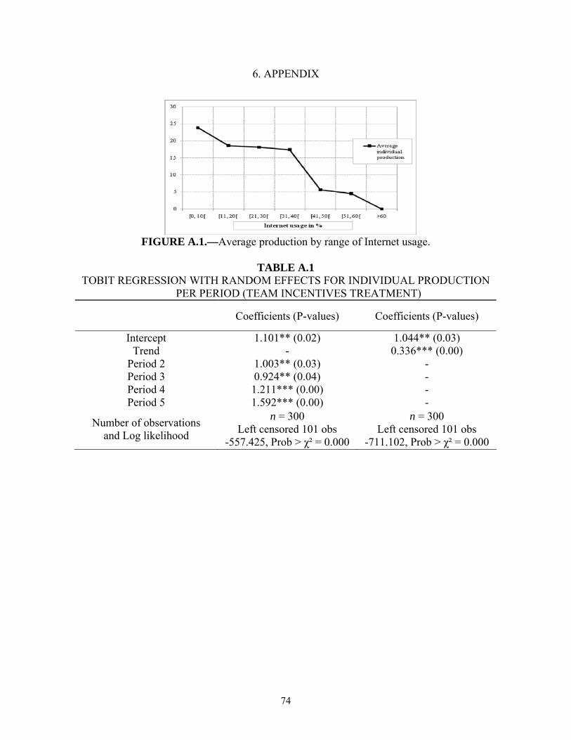
74

6. APPENDIX

FIGURE A.1.—Average production by range of Internet usage.

TABLE A.1

TOBIT REGRESSION WITH RANDOM EFFECTS FOR INDIVIDUAL PRODUCTION PER PERIOD (TEAM INCENTIVES TREATMENT)

Coefficients (P-values) Coefficients (P-values)

Intercept 1.101** (0.02) 1.044** (0.03) Trend - 0.336*** (0.00)

Period 2 1.003** (0.03) - Period 3 0.924** (0.04) - Period 4 1.211*** (0.00) - Period 5 1.592*** (0.00) -



-557.425, Prob > χ² = 0.000


-711.102, Prob > χ² = 0.000

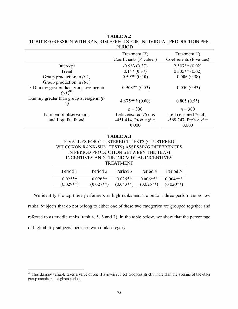
75

TABLE A.2

TOBIT REGRESSION WITH RANDOM EFFECTS FOR INDIVIDUAL PRODUCTION PER PERIOD

Treatment (T) Coefficients (P-values)

Treatment (I) Coefficients (P-values)

Intercept -0.983 (0.37) 2.507** (0.02) Trend 0.147 (0.37) 0.335** (0.02)

Group production in (t-1) 0.597* (0.10) -0.006 (0.98) Group production in (t-1)

× Dummy greater than group average in (t-1)93

-0.908** (0.03) -0.030 (0.93)

Dummy greater than group average in (t-1) 4.675*** (0.00) 0.805 (0.55)


n = 300 Left censored 76 obs -451.414, Prob > χ² =

0.000

n = 300 Left censored 76 obs -568.747, Prob > χ² =

0.000

TABLE A.3 P-VALUES FOR CLUSTERED T-TESTS (CLUSTERED

WILCOXON RANK-SUM TESTS) ASSESSING DIFFERENCES IN PERIOD PRODUCTION BETWEEN THE TEAM

INCENTIVES AND THE INDIVIDUAL INCENTIVES TREATMENT


0.025** (0.029**)

0.026** (0.027**)

0.025** (0.043**)

0.006*** (0.025**)

0.004*** (0.020**)

We identify the top three performers as high ranks and the bottom three performers as low

ranks. Subjects that do not belong to either one of these two categories are grouped together and

referred to as middle ranks (rank 4, 5, 6 and 7). In the table below, we show that the percentage

of high-ability subjects increases with rank category.

93 This dummy variable takes a value of one if a given subject produces strictly more than the average of the other group members in a given period.

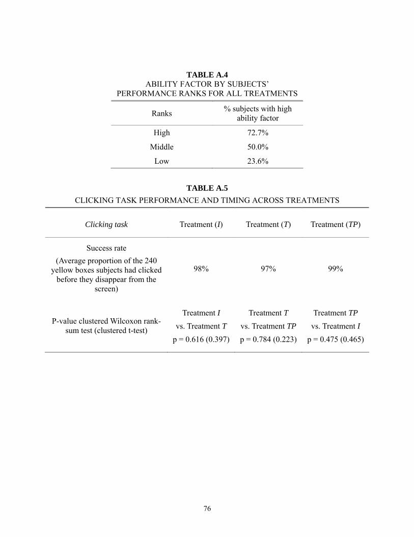
76

TABLE A.4 ABILITY FACTOR BY SUBJECTS’

PERFORMANCE RANKS FOR ALL TREATMENTS

Ranks % subjects with high ability factor

High 72.7%

Middle 50.0%

Low 23.6%

TABLE A.5 CLICKING TASK PERFORMANCE AND TIMING ACROSS TREATMENTS

Clicking task Treatment (I) Treatment (T) Treatment (TP)

Success rate (Average proportion of the 240

yellow boxes subjects had clicked before they disappear from the

screen)

98% 97% 99%

P-value clustered Wilcoxon rank-sum test (clustered t-test)

Treatment I vs. Treatment T

p = 0.616 (0.397)

Treatment T vs. Treatment TP p = 0.784 (0.223)

Treatment TP vs. Treatment I

p = 0.475 (0.465)

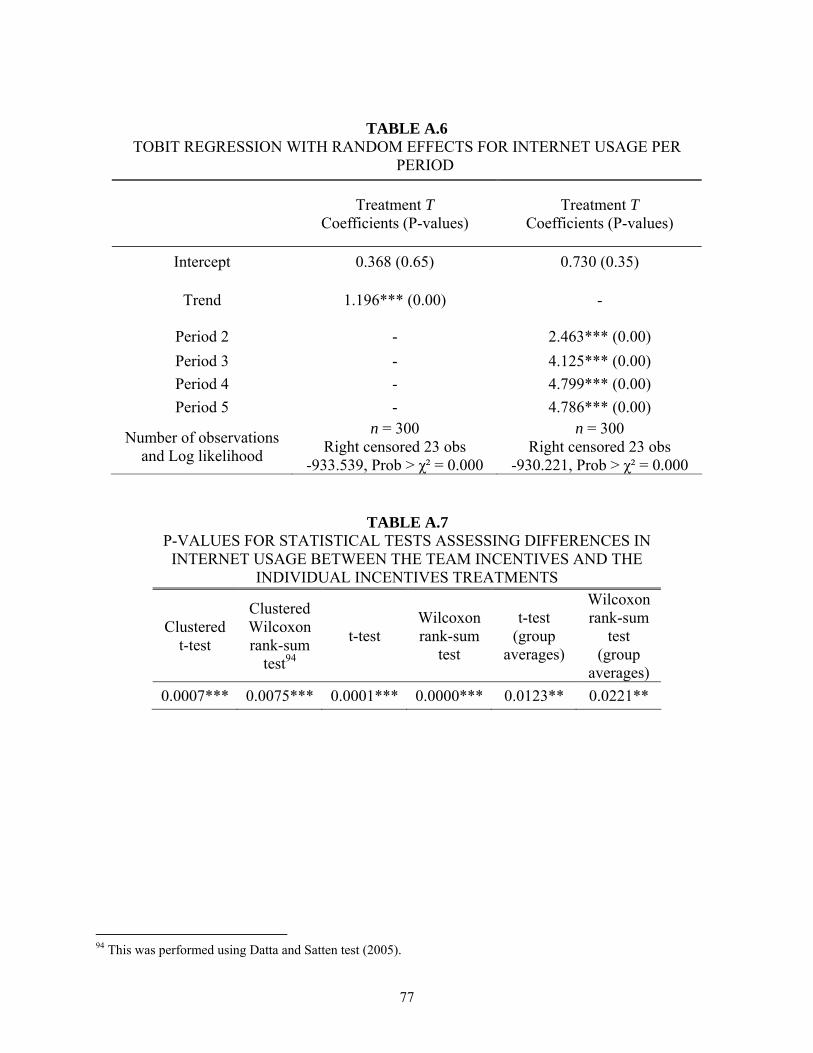
77

TABLE A.6

TOBIT REGRESSION WITH RANDOM EFFECTS FOR INTERNET USAGE PER PERIOD

Treatment T Coefficients (P-values)

Treatment T Coefficients (P-values)

Intercept 0.368 (0.65) 0.730 (0.35)

Trend 1.196*** (0.00) -

Period 2 - 2.463*** (0.00) Period 3 - 4.125*** (0.00) Period 4 - 4.799*** (0.00) Period 5 - 4.786*** (0.00)



-933.539, Prob > χ² = 0.000


-930.221, Prob > χ² = 0.000

TABLE A.7 P-VALUES FOR STATISTICAL TESTS ASSESSING DIFFERENCES IN

INTERNET USAGE BETWEEN THE TEAM INCENTIVES AND THE INDIVIDUAL INCENTIVES TREATMENTS

Clustered t-test


test94


test

t-test (group

averages)

Wilcoxon rank-sum

test (group

averages) 0.0007*** 0.0075*** 0.0001*** 0.0000*** 0.0123** 0.0221**

94 This was performed using Datta and Satten test (2005).

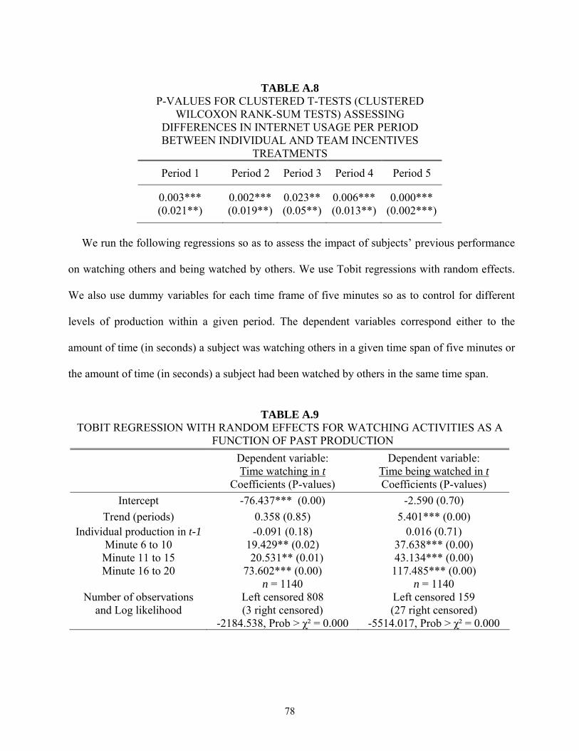
78

TABLE A.8

P-VALUES FOR CLUSTERED T-TESTS (CLUSTERED WILCOXON RANK-SUM TESTS) ASSESSING

DIFFERENCES IN INTERNET USAGE PER PERIOD BETWEEN INDIVIDUAL AND TEAM INCENTIVES

TREATMENTS


0.003*** (0.021**)

0.002*** (0.019**)

0.023** (0.05**)

0.006*** (0.013**)

0.000*** (0.002***)

We run the following regressions so as to assess the impact of subjects’ previous performance

on watching others and being watched by others. We use Tobit regressions with random effects.

We also use dummy variables for each time frame of five minutes so as to control for different

levels of production within a given period. The dependent variables correspond either to the

amount of time (in seconds) a subject was watching others in a given time span of five minutes or

the amount of time (in seconds) a subject had been watched by others in the same time span.

TABLE A.9

TOBIT REGRESSION WITH RANDOM EFFECTS FOR WATCHING ACTIVITIES AS A FUNCTION OF PAST PRODUCTION

Dependent variable: Time watching in t


Dependent variable: Time being watched in t Coefficients (P-values)

Intercept -76.437*** (0.00) -2.590 (0.70) Trend (periods) 0.358 (0.85) 5.401*** (0.00)

Individual production in t-1 -0.091 (0.18) 0.016 (0.71) Minute 6 to 10 19.429** (0.02) 37.638*** (0.00) Minute 11 to 15 20.531** (0.01) 43.134*** (0.00) Minute 16 to 20 73.602*** (0.00) 117.485*** (0.00)


n = 1140 Left censored 808 (3 right censored)

-2184.538, Prob > χ² = 0.000

n = 1140 Left censored 159 (27 right censored)

-5514.017, Prob > χ² = 0.000

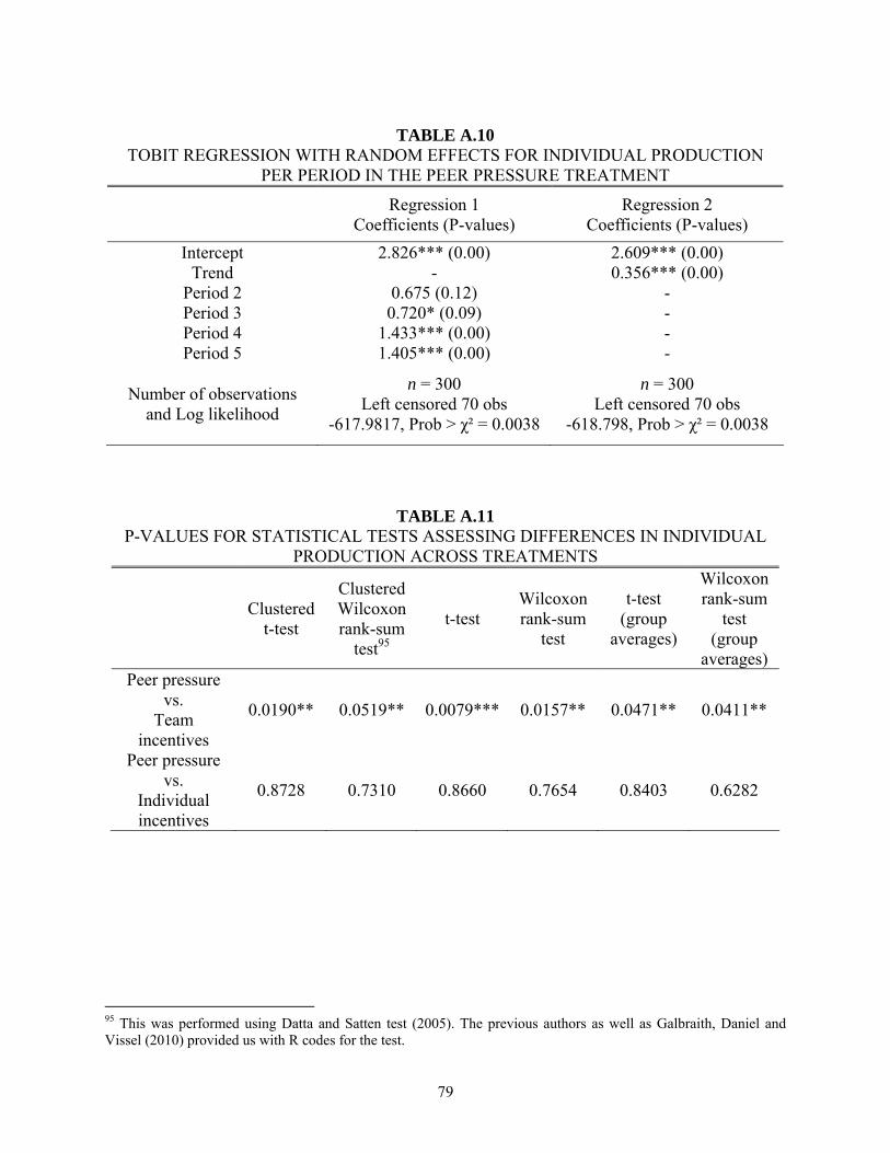
79

TABLE A.10

TOBIT REGRESSION WITH RANDOM EFFECTS FOR INDIVIDUAL PRODUCTION PER PERIOD IN THE PEER PRESSURE TREATMENT



Intercept 2.826*** (0.00) 2.609*** (0.00) Trend - 0.356*** (0.00)

Period 2 0.675 (0.12) - Period 3 0.720* (0.09) - Period 4 1.433*** (0.00) - Period 5 1.405*** (0.00) -



-617.9817, Prob > χ² = 0.0038


-618.798, Prob > χ² = 0.0038

TABLE A.11

P-VALUES FOR STATISTICAL TESTS ASSESSING DIFFERENCES IN INDIVIDUAL PRODUCTION ACROSS TREATMENTS

Clustered t-test


test95


test

t-test (group

averages)

Wilcoxon rank-sum

test (group

averages) Peer pressure

vs. Team

incentives

0.0190** 0.0519** 0.0079*** 0.0157** 0.0471** 0.0411**

Peer pressure vs.

Individual incentives

0.8728 0.7310 0.8660 0.7654 0.8403 0.6282

95 This was performed using Datta and Satten test (2005). The previous authors as well as Galbraith, Daniel and Vissel (2010) provided us with R codes for the test.

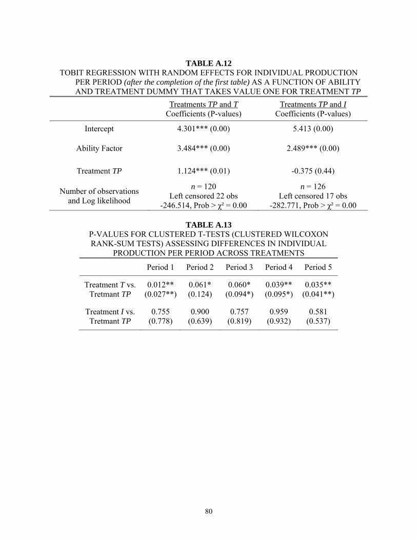
80

TABLE A.12

TOBIT REGRESSION WITH RANDOM EFFECTS FOR INDIVIDUAL PRODUCTION PER PERIOD (after the completion of the first table) AS A FUNCTION OF ABILITY AND TREATMENT DUMMY THAT TAKES VALUE ONE FOR TREATMENT TP

Treatments TP and T Coefficients (P-values)

Treatments TP and I Coefficients (P-values)

Intercept 4.301*** (0.00) 5.413 (0.00)

Ability Factor 3.484*** (0.00) 2.489*** (0.00)

Treatment TP 1.124*** (0.01) -0.375 (0.44)



-246.514, Prob > χ² = 0.00


-282.771, Prob > χ² = 0.00

TABLE A.13 P-VALUES FOR CLUSTERED T-TESTS (CLUSTERED WILCOXON RANK-SUM TESTS) ASSESSING DIFFERENCES IN INDIVIDUAL

PRODUCTION PER PERIOD ACROSS TREATMENTS


Treatment T vs. Tretmant TP

0.012** (0.027**)

0.061* (0.124)

0.060* (0.094*)

0.039** (0.095*)

0.035** (0.041**)

Treatment I vs. Tretmant TP

0.755 (0.778)

0.900 (0.639)

0.757 (0.819)

0.959 (0.932)

0.581 (0.537)

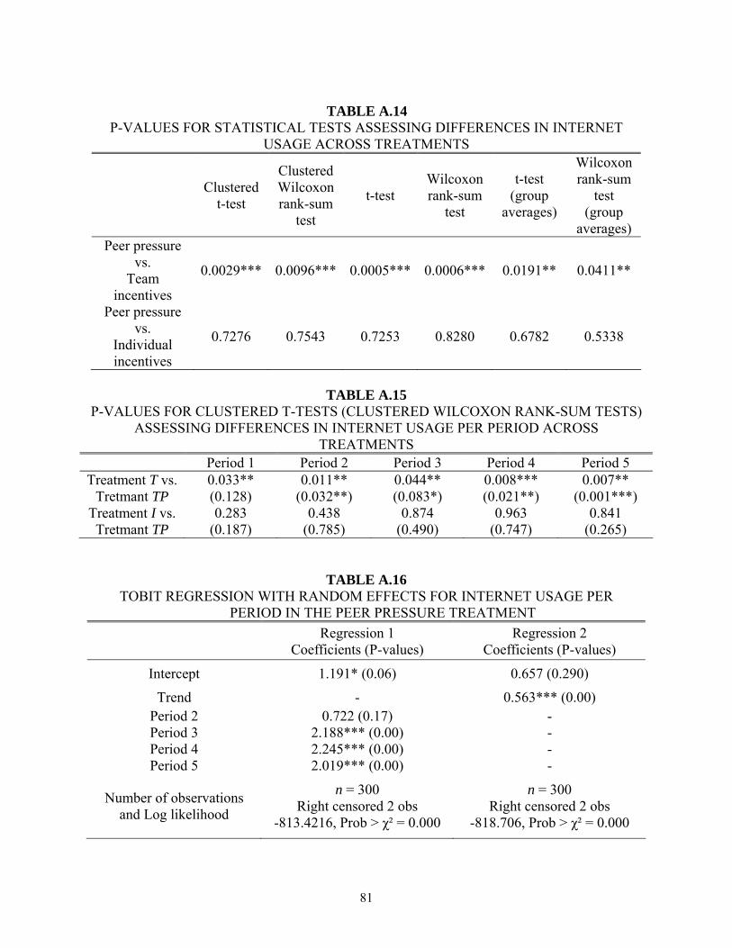
81

TABLE A.14

P-VALUES FOR STATISTICAL TESTS ASSESSING DIFFERENCES IN INTERNET USAGE ACROSS TREATMENTS

Clustered t-test


test


test

t-test (group

averages)

Wilcoxon rank-sum

test (group

averages) Peer pressure

vs. Team

incentives

0.0029*** 0.0096*** 0.0005*** 0.0006*** 0.0191** 0.0411**

Peer pressure vs.

Individual incentives

0.7276 0.7543 0.7253 0.8280 0.6782 0.5338

TABLE A.15

P-VALUES FOR CLUSTERED T-TESTS (CLUSTERED WILCOXON RANK-SUM TESTS) ASSESSING DIFFERENCES IN INTERNET USAGE PER PERIOD ACROSS

TREATMENTS Period 1 Period 2 Period 3 Period 4 Period 5

Treatment T vs. Tretmant TP

0.033** (0.128)

0.011** (0.032**)

0.044** (0.083*)

0.008*** (0.021**)

0.007** (0.001***)

Treatment I vs. Tretmant TP

0.283 (0.187)

0.438 (0.785)

0.874 (0.490)

0.963 (0.747)

0.841 (0.265)

TABLE A.16 TOBIT REGRESSION WITH RANDOM EFFECTS FOR INTERNET USAGE PER

PERIOD IN THE PEER PRESSURE TREATMENT



Intercept 1.191* (0.06) 0.657 (0.290)

Trend - 0.563*** (0.00) Period 2 0.722 (0.17) - Period 3 2.188*** (0.00) - Period 4 2.245*** (0.00) - Period 5 2.019*** (0.00) -



-813.4216, Prob > χ² = 0.000


-818.706, Prob > χ² = 0.000

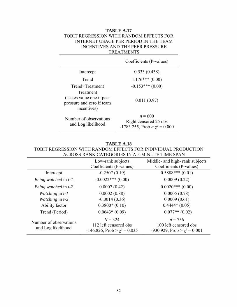
82

TABLE A.17 TOBIT REGRESSION WITH RANDOM EFFECTS FOR

INTERNET USAGE PER PERIOD IN THE TEAM INCENTIVES AND THE PEER PRESSURE

TREATMENTS


Intercept 0.533 (0.438)

Trend 1.176*** (0.00) Trend×Treatment -0.153*** (0.00)

Treatment (Takes value one if peer pressure and zero if team

incentives)

0.011 (0.97)



-1783.255, Prob > χ² = 0.000

TABLE A.18 TOBIT REGRESSION WITH RANDOM EFFECTS FOR INDIVIDUAL PRODUCTION

ACROSS RANK CATEGORIES IN A 5-MINUTE TIME SPAN

Low-rank subjects Coefficients (P-values)

Middle- and high- rank subjects Coefficients (P-values)

Intercept -0.2507 (0.19) 0.5888*** (0.01) Being watched in t-1 -0.0022*** (0.00) 0.0009 (0.22) Being watched in t-2 0.0007 (0.42) 0.0020*** (0.00)

Watching in t-1 0.0002 (0.88) 0.0005 (0.78) Watching in t-2 -0.0014 (0.36) 0.0009 (0.61) Ability factor 0.3800* (0.10) 0.4444* (0.05) Trend (Period) 0.0643* (0.09) 0.077** (0.02)


N = 324 112 left censored obs

-146.826, Prob > χ² = 0.035

n = 756 100 left censored obs

-930.929, Prob > χ² = 0.001

Economic Science Institute Working Papers

2011

11-04 Corgnet, B. and Hernán-González R. Don’t Ask Me If You Will Not Listen: The Dilemma of Participative Decision Making.

11-03 Rietz, T., Sheremeta, R., Shields, T., Smith, V. Transparency, Efficiency and the Distribution of Economic Welfare in Pass-Through Investment Trust Games.

11-02 Corgnet, B., Kujal, P. and Porter, D. The Effect of Reliability, Content and Timing of Public Announcements on Asset Trading Behavior.

11-01 Corgnet, B., Kujal, P. and Porter, D. Reaction to Public Information in Markets: How Much Does Ambiguity Matter?

2010

10-22 Mago, S., Sheremeta, R., and Yates, A. Best-of-Three Contests: Experimental Evidence.

10-21 Kimbrough, E. and Sheremeta, R. Make Him an Offer He Can't Refuse: Avoiding Conflicts Through Side Payments.

10-20 Savikhim, A. and Sheremeta, R. Visibility of Contributions and Cost of Inflation: An Experiment on Public Goods.

10-19 Sheremeta, R. and Shields, T. Do Investors Trust or Simply Gamble?

10-18 Deck, C. and Sheremeta, R. Fight or Flight? Defending Against Sequential Attacks in the Game of Siege.

10-17 Deck, C., Lin, S. and Porter, D. Affecting Policy by Manipulating Prediction Markets: Experimental Evidence.

10-16 Deck, C. and Kimbrough, E. Can Markets Save Lives? An Experimental Investigation of a Market for Organ Donations.

10-15 Deck, C., Lee, J. and Reyes, J. Personality and the Consistency of Risk Taking Behavior: Experimental Evidence.

10-14 Deck, C. and Nikiforakis, N. Perfect and Imperfect Real-Time Monitoring in a Minimum-Effort Game.

10-13 Deck, C. and Gu, J. Price Increasing Competition? Experimental Evidence.

10-12 Kovenock, D., Roberson, B.,and Sheremeta, R. The Attack and Defense of Weakest-Link Networks.

10-11 Wilson, B., Jaworski, T., Schurter, K. and Smyth, A. An Experimental Economic History of Whalers’ Rules of Capture.

10-10 DeScioli, P. and Wilson, B. Mine and Thine: The Territorial Foundations of Human Property.

10-09 Cason, T., Masters, W. and Sheremeta, R. Entry into Winner-Take-All and Proportional-Prize Contests: An Experimental Study.

10-08 Savikhin, A. and Sheremeta, R. Simultaneous Decision-Making in Competitive and Cooperative Environments.

10-07 Chowdhury, S. and Sheremeta, R. A generalized Tullock contest. 10-06 Chowdhury, S. and Sheremeta, R. The Equivalence of Contests. 10-05 Shields, T. Do Analysts Tell the Truth? Do Shareholders Listen? An Experimental Study of Analysts' Forecasts and Shareholder Reaction. 10-04 Lin, S. and Rassenti, S. Are Under- and Over-reaction the Same Matter? A Price Inertia based Account. 10-03 Lin, S. Gradual Information Diffusion and Asset Price Momentum. 10-02 Gjerstad, S. and Smith, V. Household expenditure cycles and economic cycles, 1920 – 2010. 10-01 Dickhaut, J., Lin, S., Porter, D. and Smith, V. Durability, Re-trading and Market Performance.

2009

09-11 Hazlett, T., Porter, D., Smith, V. Radio Spectrum and the Disruptive Clarity OF Ronald Coase. 09-10 Sheremeta, R. Expenditures and Information Disclosure in Two-Stage Political Contests. 09-09 Sheremeta, R. and Zhang, J. Can Groups Solve the Problem of Over-Bidding in Contests? 09-08 Sheremeta, R. and Zhang, J. Multi-Level Trust Game with "Insider" Communication. 09-07 Price, C. and Sheremeta, R. Endowment Effects in Contests. 09-06 Cason, T., Savikhin, A. and Sheremeta, R. Cooperation Spillovers in Coordination Games. 09-05 Sheremeta, R. Contest Design: An Experimental Investigation. 09-04 Sheremeta, R. Experimental Comparison of Multi-Stage and One-Stage Contests. 09-03 Smith, A., Skarbek, D., and Wilson, B. Anarchy, Groups, and Conflict: An Experiment on the Emergence of Protective Associations.

09-02 Jaworski, T. and Wilson, B. Go West Young Man: Self-selection and Endogenous Property Rights.

09-01 Gjerstad, S. Housing Market Price Tier Movements in an Expansion and Collapse.

2008

08-10 Dickhaut, J., Houser, D., Aimone, J., Tila, D. and Johnson, C. High Stakes Behavior with Low Payoffs: Inducing Preferences with Holt-Laury Gambles.

08-09 Stecher, J., Shields, T. and Dickhaut, J. Generating Ambiguity in the Laboratory.

08-08 Stecher, J., Lunawat, R., Pronin, K. and Dickhaut, J. Decision Making and Trade without Probabilities.

08-07 Dickhaut, J., Lungu, O., Smith, V., Xin, B. and Rustichini, A. A Neuronal Mechanism of Choice.

08-06 Anctil, R., Dickhaut, J., Johnson, K., and Kanodia, C. Does Information Transparency Decrease Coordination Failure?

08-05 Tila, D. and Porter, D. Group Prediction in Information Markets With and Without Trading Information and Price Manipulation Incentives.

08-04 Caginalp, G., Hao, L., Porter, D. and Smith, V. Asset Market Reactions to News: An Experimental Study.

08-03 Thomas, C. and Wilson, B. Horizontal Product Differentiation in Auctions and Multilateral Negotiations.

08-02 Oprea, R., Wilson, B. and Zillante, A. War of Attrition: Evidence from a Laboratory Experiment on Market Exit.

08-01 Oprea, R., Porter, D., Hibbert, C., Hanson, R. and Tila, D. Can Manipulators Mislead Prediction Market Observers?

Documents

Real Effort, Real Leisure and Real-time Supervision