Embed Size (px)
Citation preview

Real Analysis
Ali Ulger
September 18, 2006

ii
c© This work is licensed under the Creative Commons Attribution-NonCommercial-NoDerivs2.5 License. To view a copy of this license, visit http://creativecommons.org/licenses/by-nc-nd/2.5/ or send a letter to Creative Commons, 543 Howard Street, 5th Floor, San Francisco,California, 94105, USA.
No part of this book may be reproduced or utilized in any form or by any means, electronicor mechanical, including photocopying and recording, or by any information storage or re-trieval system, without permission in writing from the author or the license owner.
2006 Koc. University, Koc. Universitesi Rumelifeneri Kampusu, Sariyer 34450, Istanbul, Turkiye.
This book is the lecture notes of an undergraduate course on Real Analysis in Koc. Universityduring 1995-2006 given by Prof. Ali Ulger.

Contents
Preliminaries vi0.1 Sets and Mappings . . . . . . . . . . . . . . . . . . . . . . . . . . . . . . . . 10.2 Sequences and Subsequences . . . . . . . . . . . . . . . . . . . . . . . . . . . 3
0.2.1 Infinite subsets of N . . . . . . . . . . . . . . . . . . . . . . . . . . . 30.2.2 Subsequences of a Given Sequence . . . . . . . . . . . . . . . . . . . . 50.2.3 Exercises I . . . . . . . . . . . . . . . . . . . . . . . . . . . . . . . . . 7
0.3 Some Notes: . . . . . . . . . . . . . . . . . . . . . . . . . . . . . . . . . . . . 100.3.1 Exercises II . . . . . . . . . . . . . . . . . . . . . . . . . . . . . . . . 12
1 The Real Number System 151.1 Axiomatic Definition and Basic Properties of R . . . . . . . . . . . . . . . . 151.2 Intervals . . . . . . . . . . . . . . . . . . . . . . . . . . . . . . . . . . . . . . 18
1.2.1 More About Supremum and Infimum: . . . . . . . . . . . . . . . . . 191.2.2 Exercises I . . . . . . . . . . . . . . . . . . . . . . . . . . . . . . . . . 22
1.3 Convergence in R and Monotone Sequences . . . . . . . . . . . . . . . . . . . 231.4 Monotone Sequences . . . . . . . . . . . . . . . . . . . . . . . . . . . . . . . 26
1.4.1 Exercises II . . . . . . . . . . . . . . . . . . . . . . . . . . . . . . . . 291.5 Convergence of Subsequences . . . . . . . . . . . . . . . . . . . . . . . . . . 30
1.5.1 Cluster points of a Sequence . . . . . . . . . . . . . . . . . . . . . . . 301.5.2 Cauchy Sequences . . . . . . . . . . . . . . . . . . . . . . . . . . . . . 331.5.3 Exercises III . . . . . . . . . . . . . . . . . . . . . . . . . . . . . . . . 36
1.6 lim sup, lim inf . . . . . . . . . . . . . . . . . . . . . . . . . . . . . . . . . . 371.7 Elementary Topology of R . . . . . . . . . . . . . . . . . . . . . . . . . . . . 391.8 Closure and Interior of a Set . . . . . . . . . . . . . . . . . . . . . . . . . . . 43
1.8.1 Exercises IV . . . . . . . . . . . . . . . . . . . . . . . . . . . . . . . . 46
2 Minkowski and Holder Inequalities 47
3 Metric Spaces (Basic Concepts) 513.1 Metrics and Metric Spaces . . . . . . . . . . . . . . . . . . . . . . . . . . . . 513.2 Open Sets and Closed Sets . . . . . . . . . . . . . . . . . . . . . . . . . . . . 52
3.2.1 Exercises I . . . . . . . . . . . . . . . . . . . . . . . . . . . . . . . . . 553.3 Basic Topological Concepts . . . . . . . . . . . . . . . . . . . . . . . . . . . 56
iii

iv CONTENTS
3.4 Accumulation and Isolated Points of a Set . . . . . . . . . . . . . . . . . . . 59
3.4.1 Exercises II . . . . . . . . . . . . . . . . . . . . . . . . . . . . . . . . 61
3.5 Density and Separability . . . . . . . . . . . . . . . . . . . . . . . . . . . . . 62
3.5.1 Exercises III . . . . . . . . . . . . . . . . . . . . . . . . . . . . . . . . 63
3.6 Relativization . . . . . . . . . . . . . . . . . . . . . . . . . . . . . . . . . . . 64
3.6.1 Exercises IV . . . . . . . . . . . . . . . . . . . . . . . . . . . . . . . 65
3.7 Lindolf Theorem . . . . . . . . . . . . . . . . . . . . . . . . . . . . . . . . . 66
4 Convergence in a Metric Space 67
4.1 Limit and Cluster Points of a Sequence . . . . . . . . . . . . . . . . . . . . . 67
4.2 Cluster Points of a Sequence . . . . . . . . . . . . . . . . . . . . . . . . . . . 68
4.3 The set of the cluster points of a sequence xn . . . . . . . . . . . . . . . . . 69
4.4 Bolzano-Weierstrass in Rm . . . . . . . . . . . . . . . . . . . . . . . . . . . . 70
4.5 Cauchy Sequences and Completeness . . . . . . . . . . . . . . . . . . . . . . 71
4.5.1 Complete Metric Spaces . . . . . . . . . . . . . . . . . . . . . . . . . 71
4.5.2 Cluster Points of a Cauchy Sequence . . . . . . . . . . . . . . . . . . 72
5 Compactness 75
5.1 Definition and Characterization of Compact Sets . . . . . . . . . . . . . . . . 75
5.1.1 Introduction . . . . . . . . . . . . . . . . . . . . . . . . . . . . . . . . 75
5.1.2 Properties of Compact Sets: . . . . . . . . . . . . . . . . . . . . . . . 76
5.2 Second Characterization of Compact Sets . . . . . . . . . . . . . . . . . . . . 79
5.3 Totally Bounded Sets . . . . . . . . . . . . . . . . . . . . . . . . . . . . . . . 80
5.4 Exercises . . . . . . . . . . . . . . . . . . . . . . . . . . . . . . . . . . . . . . 83
6 Continuity 85
6.1 Definition . . . . . . . . . . . . . . . . . . . . . . . . . . . . . . . . . . . . . 85
6.1.1 Continuity and Compactness . . . . . . . . . . . . . . . . . . . . . . . 88
6.2 Global Characterization of the Continuity . . . . . . . . . . . . . . . . . . . 89
6.2.1 Open Mapping, Closed Mapping, Homeomorphism . . . . . . . . . . 90
6.2.2 Exercises I . . . . . . . . . . . . . . . . . . . . . . . . . . . . . . . . . 92
6.3 Uniform Continuity, Lipschitzean Mappings . . . . . . . . . . . . . . . . . . 93
6.3.1 Exercises II . . . . . . . . . . . . . . . . . . . . . . . . . . . . . . . . 95
6.4 Uniform Extension Theorem . . . . . . . . . . . . . . . . . . . . . . . . . . . 96
6.4.1 The distance function . . . . . . . . . . . . . . . . . . . . . . . . . . . 98
6.4.2 Distance Between Two Points . . . . . . . . . . . . . . . . . . . . . . 99
6.4.3 Fσ-sets, Gδ-sets in R . . . . . . . . . . . . . . . . . . . . . . . . . . . 100
6.5 Completion of a m.s. (X, d) . . . . . . . . . . . . . . . . . . . . . . . . . . . 102
6.5.1 Equivalence of Metrics . . . . . . . . . . . . . . . . . . . . . . . . . . 103

CONTENTS v
7 Limit 1077.1 Definition and Existence of Limit . . . . . . . . . . . . . . . . . . . . . . . . 107
7.1.1 Cauchy Condition For Limit . . . . . . . . . . . . . . . . . . . . . . . 1097.1.2 Limit and continuity . . . . . . . . . . . . . . . . . . . . . . . . . . . 110
7.2 Limit From the Left, From the Right . . . . . . . . . . . . . . . . . . . . . . 1107.3 Continuity of Monotone Functions . . . . . . . . . . . . . . . . . . . . . . . . 1127.4 Functions of Bounded Variation . . . . . . . . . . . . . . . . . . . . . . . . . 1137.5 Absolutely Continuous Functions . . . . . . . . . . . . . . . . . . . . . . . . 1157.6 Exercises . . . . . . . . . . . . . . . . . . . . . . . . . . . . . . . . . . . . . . 117
8 Connectedness 1198.1 Introduction: The Role of Interval in Analysis . . . . . . . . . . . . . . . . . 1198.2 Definition and Properties . . . . . . . . . . . . . . . . . . . . . . . . . . . . . 1208.3 Connected Components of a Set . . . . . . . . . . . . . . . . . . . . . . . . . 1238.4 Pointwise Connected Sets . . . . . . . . . . . . . . . . . . . . . . . . . . . . 1248.5 Some Applications . . . . . . . . . . . . . . . . . . . . . . . . . . . . . . . . 126
8.5.1 To find “fixed point theorems” . . . . . . . . . . . . . . . . . . . . . 1268.5.2 Existence of Real Roots of Polynomials . . . . . . . . . . . . . . . . . 1268.5.3 The Structure of Open Sets in R . . . . . . . . . . . . . . . . . . . . 1278.5.4 To find if given two metric spaces are homeomorphic or not . . . . . 127
8.6 Exercises . . . . . . . . . . . . . . . . . . . . . . . . . . . . . . . . . . . . . . 128
9 Numerical Series 1299.1 Generalities about Series . . . . . . . . . . . . . . . . . . . . . . . . . . . . . 1299.2 Tests of convergence for positive series . . . . . . . . . . . . . . . . . . . . . 1329.3 Absolute and Unconditional Convergence . . . . . . . . . . . . . . . . . . . . 138
9.3.1 Absolutely Convergent vs. Unconditionally Convergent . . . . . . . . 1409.4 Abel and Dirichlet Tests . . . . . . . . . . . . . . . . . . . . . . . . . . . . . 1439.5 Product of Series . . . . . . . . . . . . . . . . . . . . . . . . . . . . . . . . . 145
9.5.1 Cauchy Method of Sum . . . . . . . . . . . . . . . . . . . . . . . . . 1479.6 Exercises . . . . . . . . . . . . . . . . . . . . . . . . . . . . . . . . . . . . . . 149
10 Sequences and Series of Functions 15110.1 Sequences of Functions . . . . . . . . . . . . . . . . . . . . . . . . . . . . . . 151
10.1.1 Pointwise Convergence . . . . . . . . . . . . . . . . . . . . . . . . . . 15110.1.2 Uniform Convergence . . . . . . . . . . . . . . . . . . . . . . . . . . 153
10.2 Continuity, Differentiation and Integration . . . . . . . . . . . . . . . . . . . 15510.2.1 Uniform Convergence and Continuity . . . . . . . . . . . . . . . . . . 15510.2.2 Metric Nature of Uniform Convergence . . . . . . . . . . . . . . . . . 15610.2.3 Uniform Convergence and Integration . . . . . . . . . . . . . . . . . . 15610.2.4 Uniform Convergence and Differentiation . . . . . . . . . . . . . . . . 157
10.3 Series of Functions . . . . . . . . . . . . . . . . . . . . . . . . . . . . . . . . 15810.3.1 Pointwise Convergence of Function Series . . . . . . . . . . . . . . . . 158

vi CONTENTS
10.3.2 Uniform Convergence of the Function Series . . . . . . . . . . . . . . 15910.3.3 Hereditary Properties . . . . . . . . . . . . . . . . . . . . . . . . . . . 160
10.4 Tests for Uniform Convergence . . . . . . . . . . . . . . . . . . . . . . . . . . 16110.4.1 Abel and Dirichlet Tests for Uniform Convergence . . . . . . . . . . . 162
10.5 Power Series and Taylor Expansion . . . . . . . . . . . . . . . . . . . . . . . 16410.5.1 Radius of Convergence of a Power Series . . . . . . . . . . . . . . . . 16510.5.2 Differentiation and Integration of Power Series . . . . . . . . . . . . . 16710.5.3 Analytic Functions . . . . . . . . . . . . . . . . . . . . . . . . . . . . 16910.5.4 Continuity at the Boundary of Interval of Convergence . . . . . . . . 170
10.6 Continuous but Nowhere Differentiable Functions . . . . . . . . . . . . . . . 17210.7 Exercises . . . . . . . . . . . . . . . . . . . . . . . . . . . . . . . . . . . . . . 175
11 Riemann Integral 17911.1 Definition and Existence . . . . . . . . . . . . . . . . . . . . . . . . . . . . . 17911.2 Properties of the Riemann Integral . . . . . . . . . . . . . . . . . . . . . . . 18411.3 Fundamental Theorem of Calculus . . . . . . . . . . . . . . . . . . . . . . . 18611.4 Improper Integrals . . . . . . . . . . . . . . . . . . . . . . . . . . . . . . . . 18811.5 Exercises . . . . . . . . . . . . . . . . . . . . . . . . . . . . . . . . . . . . . . 190
12 The Space C(K) 19512.1 Generalities About C (K) . . . . . . . . . . . . . . . . . . . . . . . . . . . . 195
12.1.1 Cantor’s Diagonal Method . . . . . . . . . . . . . . . . . . . . . . . . 19512.1.2 Pointwise and Uniformly Bounded Sets of Functions . . . . . . . . . . 19612.1.3 Equi-continuity of a set of Functions . . . . . . . . . . . . . . . . . . 197
12.2 Ascoli - Arzela Theorem . . . . . . . . . . . . . . . . . . . . . . . . . . . . . 19812.3 Stone - Weierstrass Theorem . . . . . . . . . . . . . . . . . . . . . . . . . . . 20012.4 Exercises . . . . . . . . . . . . . . . . . . . . . . . . . . . . . . . . . . . . . . 205
13 Baire Category Theorem 20713.1 Generalities . . . . . . . . . . . . . . . . . . . . . . . . . . . . . . . . . . . . 20713.2 Basic Notations . . . . . . . . . . . . . . . . . . . . . . . . . . . . . . . . . . 208
13.2.1 Gδ-sets, Fσ-sets . . . . . . . . . . . . . . . . . . . . . . . . . . . . . . 20813.2.2 Nowhere Dense Sets . . . . . . . . . . . . . . . . . . . . . . . . . . . 20813.2.3 First and Second Category Sets, Residual Sets . . . . . . . . . . . . . 209
13.3 Various Forms of the Baire Category Theorem . . . . . . . . . . . . . . . . . 21013.4 A Study of Discontinuous Functions (Baire’s Great Theorem) . . . . . . . . 212
13.4.1 Continuity of Baire-1 Functions . . . . . . . . . . . . . . . . . . . . . 21313.5 Exercises . . . . . . . . . . . . . . . . . . . . . . . . . . . . . . . . . . . . . . 216

PRELIMINARIES
1. Sets and Mappings
2. Sequences and Subsequences
0.1 Sets and Mappings
Let X be any set, by 2X we denote the set of all subsets of X. A ⊆ X ⇔ A ∈ 2X .
If A ⊆ X by AC we shall denote the complement of A in X.
AC = {x ∈ X, x /∈ A} = X − A
Now let I be an index set. Suppose that for each α ∈ I, we have a set Aα.
Then the collection of Aα, α ∈ I is said to be a family of sets.
For such a family, if I �= ∅ , for α ∈ I, ∪Aα and ∩Aα are defined by:
∪Aα = {x : ∃α ∈ I x ∈ Aα}
∩Aα = {x : ∀α ∈ I x ∈ Aα}Now suppose that Aα ⊆ X . Then,
(∪Aα)C = ∩ACα
(∩Aα)C = ∪ACα
(De Morgan’s Law)
Now let Y be another set and f : X → Y be a mapping.
1
2 CONTENTS
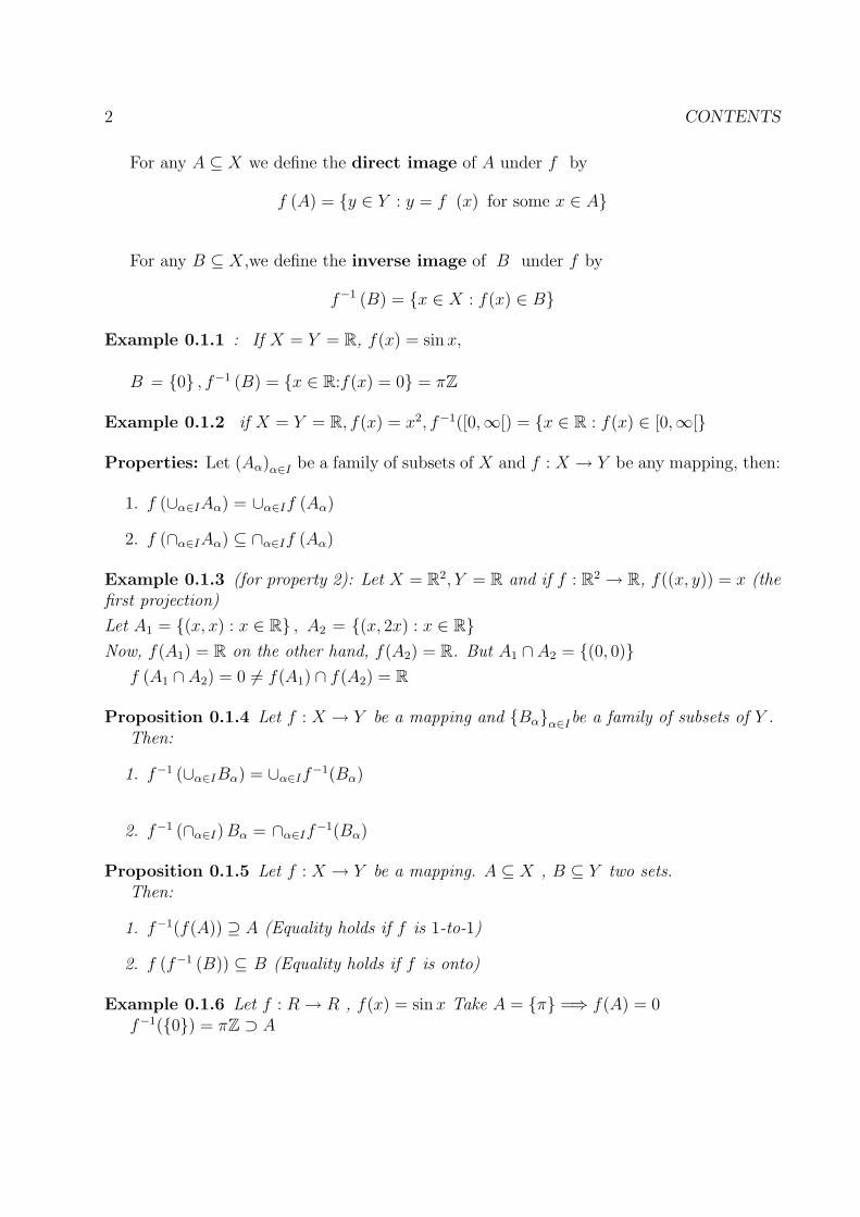
For any A ⊆ X we define the direct image of A under f by
f (A) = {y ∈ Y : y = f (x) for some x ∈ A}
For any B ⊆ X,we define the inverse image of B under f by
f−1 (B) = {x ∈ X : f(x) ∈ B}
Example 0.1.1 : If X = Y = R, f(x) = sin x,
B = {0} , f−1 (B) = {x ∈ R:f(x) = 0} = πZ
Example 0.1.2 if X = Y = R, f(x) = x2, f−1([0,∞[) = {x ∈ R : f(x) ∈ [0,∞[}
Properties: Let (Aα)α∈I be a family of subsets of X and f : X → Y be any mapping, then:
1. f (∪α∈IAα) = ∪α∈If (Aα)
2. f (∩α∈IAα) ⊆ ∩α∈If (Aα)
Example 0.1.3 (for property 2): Let X = R2, Y = R and if f : R2 → R, f((x, y)) = x (thefirst projection)
Let A1 = {(x, x) : x ∈ R} , A2 = {(x, 2x) : x ∈ R}Now, f(A1) = R on the other hand, f(A2) = R. But A1 ∩ A2 = {(0, 0)}
f (A1 ∩ A2) = 0 �= f(A1) ∩ f(A2) = R
Proposition 0.1.4 Let f : X → Y be a mapping and {Bα}α∈Ibe a family of subsets of Y .Then:
1. f−1 (∪α∈IBα) = ∪α∈If−1(Bα)
2. f−1 (∩α∈I) Bα = ∩α∈If−1(Bα)
Proposition 0.1.5 Let f : X → Y be a mapping. A ⊆ X , B ⊆ Y two sets.Then:
1. f−1(f(A)) ⊇ A (Equality holds if f is 1-to-1)
2. f (f−1 (B)) ⊆ B (Equality holds if f is onto)
Example 0.1.6 Let f : R → R , f(x) = sin x Take A = {π} =⇒ f(A) = 0f−1({0}) = πZ ⊃ A

0.2. SEQUENCES AND SUBSEQUENCES 3
Example 0.1.7 Let f : R → R , f(x) = x2
B = [0, +∞[ =⇒ f−1(B) = RThen f (f−1 (B)) = f(R) = B
Example 0.1.8 Let f : R → R , f(x) = sin x Let B = {0, 2} f−1(B) = πZf (f−1(B)) = f(πZ) = {0} ⊂ {0, 2}
Remark: Let f : X → Y be a mapping.
If A ⊆ X =⇒ f(Ac) �= f(A)c (= if f is bijective)
But for B ⊆ Y f−1(Bc) = f−1(B)C
0.2 Sequences and Subsequences
The set N = {1, 2, ....} is the set of the positive integers.
Definition 0.2.1 Let X be any set, X �= Ø. Any mapping Γ : N → X is said to be asequence in X.
Let for each n ∈ N , xn = Γ(n). Then instead of Γ(n) we usually write (xn)n∈N and saythat (xn)n∈N is a sequence in X.
The set Γ (N) = {xn : n ∈ N} ⊆ X is the range of Γ.
Remark: Do not confuse Γ which is a mapping with its range. It is a set !
Example 0.2.2 Let X = R, Γ : N → R
Γ(n) = n2 Γ(n) = n Γ(n) = ln(n + 1) Sequences in R.
0.2.1 Infinite subsets of N
Let � ={F ∈ 2N : F is an infinite set
}. What is card�?
Let p & q be two prime numbers, (p �= q), then ∀n,m ∈ N \ {0} , pn �= qm (∗)
Let p0, p1, p2, . . . , pk, . . . be distinct prime numbers.
Let for each k = 0, 1, 2, . . . , Fk ={pn+1
k : n ∈ N}. If pk = 2 =⇒ Fk = {2,22,23, . . . .}
Hence (∗) shows that for i �= j, Fi ∩ Fj = ∅. Moreover, each Fi is an infinite set.

4 CONTENTS
Let also �0 = {A ∈ 2n : A is finite}
�0 ∩ � = ∅
�0 ∪ � = 2N
Proposition 0.2.3 �0 is countable.
Proof 0.2.4 For every n ∈ N, Nn = N × N × N× · · ·×N is a countable set.
So, Y = ∪n∈NNn is also countable.
Now we define a mapping f : �0 → Y as follows:
Let A ∈ �0. So A is of the form: A = {n1, n2, n3, . . . , nk, . . .}
f(A) = (n1, n2, . . . , nk) ∈ Nk. Clearly f is 1 − to − 1. As Y is countable , so is �0.
Conclusion: The set �is uncountable.Thus in N there are uncountably many infinite subsets.
Definition 0.2.5 A mapping Γ : N → N is said to be strictly increasing if whenevern < m we have Γ(n) < Γ(m)
Example 0.2.6 LetΓ : N → N, Γ(n) = 2nΓ : N → N, Γ(n) = 3n + 1Γ : N → N, Γ(n) = n2 + n + 1
are strictly increasing mappings.
Question: How many strictly increasing mappings Γ : N → N do we have?
*If Γ : N → N is strictly increasing, then the set � = Γ(N) is an infinite set.
**Now let � ⊆ N be an infinite set. So � is of the form � = {n0, n1, ....} with n0 <n1 < n2 < . . .
To �, we associate the mapping Γ : N → N ,Γ(k) = nk so that Γ(N) = �.
The above two points “*” and “**” show that there are uncountably many strictly increasingmappings.

0.2. SEQUENCES AND SUBSEQUENCES 5
0.2.2 Subsequences of a Given Sequence
Definition 0.2.7 Let Γ : N → X be any sequence and Ψ : N → N be a strictly increasingmapping. Γ◦Ψ : N → X is also a sequence. The sequence Γ◦Ψ is said to be a subsequenceof Γ.
Hence any sequence Γ has uncountably many subsequences.
Practical notation for subsequences: Let Γ = (xn)n∈N be a sequence. (Γ : N → X,xn = Γ(n))
Let Ψ : N → N be a strictly increasing mapping.
Let nk = Ψ(k) so that n0 < n1 < n2 < . . . < nk < . . . then, Γ ◦ Ψ(k) = xnk, and
k → ∞ =⇒ nk → ∞
So, (xnk)k∈N is a subsequence of (xn)n∈N
If we put yk = xnkis a sequence of its own , i.e. (yk)k∈N is a sequence.
So, if (xn)n∈N is a sequence in a set and n0 < n1 < n2 < . . . < nk are given integers.
Taking yk = xnkwe obtain a new sequence (yk)k∈N. This later sequence is said to be a
subsequence of (xn)n∈N .
Observe that {xn0 , xn1 , xn2 , .........} ⊆ {x0,x1,x2........}
Example 0.2.8 If X = R, xn = 1n2+1 and n0 < n1 < n2 < . . . < nk < . . . is any sequence
of integers.
yk = 1(nk)2+1 , is a subsequence of xn.
So, for instance, if nk = 3k + 5 ⇒ n0 = 5, n1 = 8, n2 = 11,. . .
then, xnk=
1
(3k + 5)2 + 1and it takes such values for given nk’s.

6 CONTENTS
x0 = 1 xn0 =1
26
x1 = 12
xn1 =1
65
x2 = 15
xn2 =1
122
Example 0.2.9 • Consider the sequence (xn)n∈N that goes as follows:
0, 1, 2, 3, 4, 0, 1, 2, 3, 4, 0, 1, 2, 3, 4, . . .
Give at least three subsequences of that sequence.
1. x0 → xn0
2. x5 → xn1
3. x10 → xn2
• For the sequence xn = (−1)n Find at least three subsequences.
(x2n)n∈N is a subsequence
(x2n+1)n∈N is a subsequence
(x3n+2)n∈N is a subsequence
Remark:
• Let (xn)n∈N be a sequence in X. If x0 = x1 = x2 = . . . = xk = . . ., then we say that,(xn)n∈N is a constant sequence.
• If there exists N ∈ N ∀n ≥ N, xN = xn = xn+1 = . . . then we say, (xn)n∈Nis almostconstant.
0.2. SEQUENCES AND SUBSEQUENCES 7
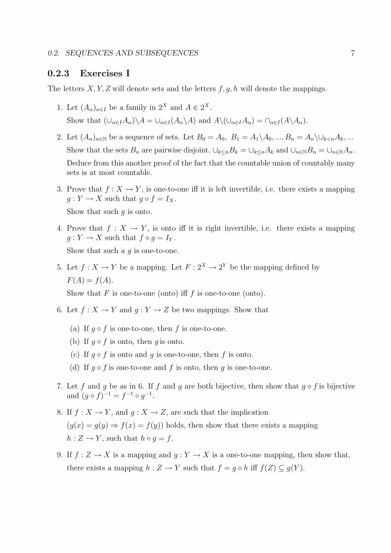
0.2.3 Exercises I
The letters X,Y, Z will denote sets and the letters f, g, h will denote the mappings.
1. Let (Aα)α∈I be a family in 2X and A ∈ 2X .
Show that (∪α∈IAα)\A = ∪α∈I(Aα\A) and A\(∪α∈IAα) = ∩α∈I(A\Aα).
2. Let (An)n∈N be a sequence of sets. Let B0 = A0, B1 = A1\A0, ..., Bn = An\∪k<nAk, ...
Show that the sets Bn are pairwise disjoint, ∪k≤nBk = ∪k≤nAk and ∪n∈NBn = ∪n∈NAn.
Deduce from this another proof of the fact that the countable union of countably manysets is at most countable.
3. Prove that f : X → Y , is one-to-one iff it is left invertible, i.e. there exists a mappingg : Y → X such that g ◦ f = IX .
Show that such g is onto.
4. Prove that f : X → Y , is onto iff it is right invertible, i.e. there exists a mappingg : Y → X such that f ◦ g = IY .
Show that such a g is one-to-one.
5. Let f : X → Y be a mapping. Let F : 2X → 2Y be the mapping defined by
F (A) = f(A).
Show that F is one-to-one (onto) iff f is one-to-one (onto).
6. Let f : X → Y and g : Y → Z be two mappings. Show that
(a) If g ◦ f is one-to-one, then f is one-to-one.
(b) If g ◦ f is onto, then g is onto.
(c) If g ◦ f is onto and g is one-to-one, then f is onto.
(d) If g ◦ f is one-to-one and f is onto, then g is one-to-one.
7. Let f and g be as in 6. If f and g are both bijective, then show that g ◦ f is bijectiveand (g ◦ f)−1 = f−1 ◦ g−1.
8. If f : X → Y , and g : X → Z, are such that the implication
(g(x) = g(y) ⇒ f(x) = f(y)) holds, then show that there exists a mapping
h : Z → Y , such that h ◦ g = f .
9. If f : Z → X is a mapping and g : Y → X is a one-to-one mapping, then show that,
there exists a mapping h : Z → Y such that f = g ◦ h iff f(Z) ⊆ g(Y ).

8 CONTENTS
10. For A ⊆ X, let χA : X → {0, 1} be the mapping defined by χA(x) =
{1 if x ∈ A0 if x /∈ A
Show that the following holds.
(a) χA = 0 iff A = ∅.(b) χA = 1 iff A = X.
(c) χA = χB iff A = B.
(d) χA∪B = χA + χB − χA × χB and χA∩B = χA × χB.
(e) χAc = 1 − χA.
(f) χA∆B = |χA − χB|, where A∆B = (A\B) ∪ (B\A).
(g) χA∆B = χA + χB (mod 2)
11. Let F (X; {0, 1}) be the set of the mappings f : X → {0, 1}.Show that there exists a bijection between the sets F (X; {0, 1}) and 2X .
12. Let S be the set of all the sequences in the set {0, 1}. Show that the set S is uncount-able.
13. Let F = {A ∈ 2N : both A, and Ac, are infinite}. Show that the set F is uncountable.
14. Suppose that the sets X and Y are infinite and f : X → Y is an onto mapping suchthat, for each y ∈ Y , the set f−1({y}) is countable.
Show that then Card(X) = Card(Y ).
15. Let F = {A ∈ 2N : A �= ∅ and finite}. Let ϕ : F → N, ϕ(A) =∑n∈A
n.
Show that ϕ is onto and that, for each n ∈ N (n ≥ 1), the set ϕ−1(n) is finite.
From this deduce another proof of the fact that F is countable.
16. Suppose that X is infinite and F is the set of the finite subsets of X. Show thatCard(X) = Card(F ).
17. Show that A is infinite iff it has a proper subset B such that Card(A) = Card(B).
18. Let p1, p2, . . . be prime numbers. Let Fk = {(pk)n+1 : n ∈ N}.
Show that the sets F1, F2, ... are infinite and pairwise disjoint.
Deduce that any sequence (xn)n∈N in a set X has infinitely many subsequences withpairwise disjoint index sets.
19. Let A0, A1, ... be nonempty subsets of X. Put A∗ = ∩n∈N∪k≥nAk and A∗ = ∪n∈N∩k≥nAk.

0.2. SEQUENCES AND SUBSEQUENCES 9
(a) Show that A∗ ⊆ A∗ and that A∗ = A∗ if the sequence of the sets (An)n∈N ismonotone.
(b) Let x ∈ X be a given point. Show that
i. x ∈ A∗ iff x ∈ An for infinitely many n ∈ N.
ii. x ∈ A∗ iff x ∈ An for all but finitely many n ∈ N.
(c) Explain the difference between the sentences in 19(b)i and 19(b)ii.
20. Let (X,≤) be an ordered set such that for any two elements x, y in X, sup{x, y} andinf{x, y} exist.
Let f : X → X be a mapping. Show that f is increasing iff f(inf{x, y}) ≤ inf f({x, y}),for every x, y in X.
21. Let (xn, yn)(n,n)∈N×N be a sequence in X × X and A and B be two infinite subsets ofN.
Is the sequence (xk, yp)(k,p)∈A×B a subsequence of (xn, yn)(n,n)∈N×N?
10 CONTENTS
0.3 Some Notes:
Definition 0.3.1 Let X (�= ∅) be a set and ≤ be a binary relation in X.≤ is said to be an order relation, if it is reflexive, antisymmetric, transitive.
The set X equipped with an order relation is said to be an ordered set.
Example 0.3.2 1. N, Z, Q, R are ordered under the usual “less than”, ≤.
2. Let E be any set and X = 2E
For A,B ∈ X let A � B iff A ⊆ B then, � is a n order relation on X, known asinclusion relation.
3. Let X = F (N,N) be the set of all mappings: Γ : N→N.
We define a binary relation � on X as follows:
Γ ≤ Ψ iff Γ(n) ≤ Ψ(n) ∀ n ∈ N. Then ≤ is an order relation on N.
Definition 0.3.3 Now, let (X,�) be an ordered set and A ⊆ X, (A �= ∅).We say that,
1. A is bounded from above, if there is an m ∈ X ∀a ∈ A, a � m.
Such an m is said to be an upper bound for A. Of course any m′ ∈ X, m � m′ isalso an upper bound.
For instance, Q and N are not bounded from above.
Now let A = {x ∈ Q, x2 � 2} Then, A is bounded from above.
2. A is bounded from below if ∃n ∈ X ∀a ∈ A, n � a
In this case, n is said to be a lower bound for A. Of course any n′ � n is also alower bound for A.
For instance, N is bounded from below.
But Q and Z are not bounded from below.
3. A is bounded, if A ⊆ X is both bounded from above and below.
Hence, A is bounded if ∃n,m ∈ X, ∀x ∈ A, n � x � m
4. A has a greatest element if there is an element α ∈ A ∀x ∈ X, x � α
A has a a smallest element if there is an element β ∈ A ∀x ∈ A, β � x
Example 0.3.4 If X = Q, A = N then A has a smallest element namely β = 0 but it hasno greatest element.
If X = N, A ⊆ N A �= ∅ then A has a smallest element

0.3. SOME NOTES: 11
Definition 0.3.5 Let A ⊆ X be a set.We say that, A has a least upper bound
if ∃α ∈ X {
i) ∀x ∈ A, x ≤ α
ii) ∀β ∈ Xsatisfying “ ∀x ∈ A, x ≤ β”, α ≤ β.
In this case ,we write, α = sup A or α = lubA
Thus, α = sup A ⇔{
(1) ∀x ∈ A, x ≤ α
(2) ∀β ∈ X, if for all x ∈ A, x ≤ β then α ≤ β.
If X = Q, A = {x ∈ Q : x2 ≤ 2}. Does A have a least upper bound?
Definition 0.3.6 Let A ⊆ X we say that A has a greatest lower bound if
∃β ∈ X :
{(i) ∀x ∈ A, x ≥ β,
(ii) ∀γ ∈ X satisfying “ ∀x ∈ A, x ≥ γ” γ ≤ β.
If A has a greatest element α, then α = sup A, conversely, if α = sup A and α ∈ A ⇒ αis the greatest element of A.
Similarly, if A has a smallest element β then β = inf A.

12 CONTENTS
0.3.1 Exercises II
1. Find at least 3 different subsequences of the sequence
x0 x1 x2 x3 x4 .......................................↓ ↓ ↓ ↓ ↓0, 1, 2, 3, 0, 1, 2, 3, 0, 1, 2, 3, 0, ...
2. Find at least 2 different subsequences of the sequence
x0 x1 x2 x3 ......................↓ ↓ ↓ ↓1, 1
2, 3, 1
4, 5, 1
6, 7, 1
8, ...
3. Let x, y, z be 3 real numbers. Put x+ = max{x, 0} and x− = min{−x, 0}.Prove the following:
(a) x = x+ − x−
(b) |x| = x+ + x−
(c) x + y = max{x, y} + min{x, y}(d) sup{x, y} + z = sup{x + z, y + z}(e) min{x, y} + z = min{x + z, y + z}(f) x ≤ y iff x+ ≤ y+ and x− ≤ y−
(g) sup{x, y} = − inf{−x,−y}(h) max{x, y} = max{x − y, 0} + y = (x − y)+ + y =
|x − y| + x + y
2.
(i) min{x, y} = min{x − y, 0} + y = −(x − y)− + y =x − y − |x − y|
2.
4. Let X be an infinite set. Let F be the set of all the finite subsets of X.
Show that CardF = CardX.
5. Show that N contains infinitely many infinite sets A0, A1, ..., An, ... such that Ai∩Aj = ∅for i �= j.
6. Let a = (a1, ..., an) ∈ Rn be a fixed element, 1 ≤ p < ∞ and ||x||p = [|a1|p + ... + |an|p]1p .
Show that limp→∞||a||p = max{|a1|, |a2|, ..., |an|}.7. Let A and B be 2 nonempty subsets of R.
Let A + B = {a + b : a ∈ A, b ∈ B}, A × B = {a × b : a ∈ A, b ∈ B}. Show that
(a) if A and B are bounded from above (or below), then so are the sets A + B, A ×B, A ∪ B, A ∩ B.
0.3. SOME NOTES: 13
(b) if A is bounded from above, then so is every nonempty subsets of A.
8. Let A and B be 2 nonempty subsets of R. Assume that both of them are bounded.Show that
(a) if A ⊆ B, then sup A ≤ sup B and inf A ≥ inf B.
(b) sup(A + B) = sup A + sup B.
(c) sup{|a| × |b| : a ∈ A, b ∈ B} ≤ sup{|a| : a ∈ A} × sup{|b| : b ∈ B}.
Give an example showing that in 8c in general we do not have equality.

14 CONTENTS

Chapter 1
The Real Number System
1. Axiomatic definition and basic Properties of R
2. Convergence in R and monotone sequences
3. Bolzano-Weierstrass Theorem
4. Cauchy sequences
5. lim sup, lim inf
6. Elementary topology of R
“ God created the real numbers, we learn its properties.”
1.1 Axiomatic Definition and Basic Properties of R
There exists a set R called the set of real numbers, satisfying the following axioms:
Axiom 1.1.1 (Algebraic Structure) (R, +, .) is a field and it contains Q as a subfield.
We denote the natural element of R for + by 0.
The inverse for x �= 0 for multiplication by1
x, for addition by −x.
Axiom 1.1.2 (Order Structure) There exists an order relation on (R,≤) extending thatof Q, which is total (i.e., ∀x, y ∈ R, x ≤ y or y ≤ x) and which is consistent with thealgebraic structure. This means that,
1. x ≤ y =⇒ (∀z ∈ R) x + z ≤ y + z
2. x ≤ y and z ≥ 0 =⇒ xz ≤ yz
15

16 CHAPTER 1. THE REAL NUMBER SYSTEM
Axiom 1.1.3 (Supremum) Any nonempty set A ⊆ R, which is bounded from above, hasa supremum α ∈ R i.e. there is a number α ∈ R such that:
1. ∀ x ∈ A, x ≤ α
2. ∀ ε > 0, ∃ xε ∈ A, xε > α − ε
For any A ⊆ X,
α = sup A ⇐⇒{
1) ∀ x ∈ A,x ≤ α2) ∀ β ∈ X, if ∀x ∈ A, x ≤ β, then α ≤ β
This α is said to be the supremum of A and denoted by α = sup A. Thus,
α = sup A ⇐⇒{
1) ∀ x ∈ A, x ≤ α2) ∀ ε > 0, ∃ xε ∈ A, xε > α − ε
Example 1.1.4 Let A = {x ∈ Q : x2 < 2}. Then, A ⊆ R. A is bounded from above, henceby the supremum axiom, A has a supremum in R. Let α = sup A.
Let us see that x =√
2.
1. ∀x ∈ A, x <√
2
2. Let ε > 0 be any number. So, for xε ∈ A, xε >√
2 − ε.
2 > x2ε >
(√2 − ε
)2
= 2 − 2√
2ε + ε2︸ ︷︷ ︸ε(2√
2 − ε)
> 0︸ ︷︷ ︸2√
2 − ε > 0
ε < 2√
2
You can always find xε ∈ A xε >√
2 − ε. So, sup A =√
2.
Example 1.1.5 Let A =
{n
n + 1: n = 1, 2, 3, ..
}. Then A is bounded from above, so
α = sup A exists. Let us see that α = 1. Indeed,
1. ∀n ≥ 0,n
n + 1≤ 1
2. Let ε � 0 be any number, then the inequalityn
n + 1> 1 − ε has a solution nε. Then,
xε =nε
nε + 1> 1 − ε.
Proposition 1.1.6 A nonempty subset B ⊆ R, which is bounded below has an infimumβ ∈ R.
1.1. AXIOMATIC DEFINITION AND BASIC PROPERTIES OF R 17
Proof 1.1.7 We are going to show that, there is a number β ∈R such that:
1. ∀x ∈ B, β ≤ x
2. ∀ ε > 0, ∃ xε ∈ B : xε < β + ε
Let A = {−x : x ∈ B} . Then A is bounded from above, so by supremum axiom 1.1.3∃α ∈ R α = sup A.
=⇒ 1)∀x ∈ B,−x ≤ α2)∀ε > 0,∃ x
ε∈ B : −x
ε≥ α − ε
This is equivalent to,
=⇒ 1)∀x ∈ B, x ≥ −α2)∀ ε � 0,∃ x
ε∈ B : −x
ε≤ −α + ε
Hence −α is the infimum of B.
At the same time we have proved that,
sup (−B) = − inf(B) (for any set B bounded from below)inf (−A) = − sup(A) (for any set A bounded from above)
Proposition 1.1.8 Given any x ∈ R, x ≥ 0, there is a unique n ∈ N n − 1 < x ≤ n.
Proof 1.1.9 Let A = {n ∈ N : n ≥ x}. Then, A �= ∅.
A ⊆ N =⇒A has a smallest element, call it n.
Thus, n ∈ A, but n − 1 /∈ A. So, n ≥ x, but n − 1 < x, i.e. n − 1 < x ≤ n
Proposition 1.1.10 (Archimedian Property of R): Given any ε > 0, there is N ∈ Nsuch that N.ε > 1.
Proof 1.1.11 Observe that, N.ε > 1 is equivalent to1
N< ε.
Let in the Proposition 1.1.8, x =1
ε. Then, there is n ∈ N such that N − 1 ≤ 1
ε< N.
Hence,1
N< ε.
Proposition 1.1.12 (Density of Q in R): Given any x ∈ R and any ε > 0 there is anr ∈ Q such that |x − r| < ε.
Proof 1.1.13 If x ∈ Q, then take r = x. Suppose x > 0.
By the Proposition 1.1.10, there is an N ∈ N 1
N< ε. Consider the number Nx.
By the Proposition 1.1.8, applies to Nx, there is an integer n ∈ N, n < Nx ≤ n + 1.
Let r =n
N, then r ∈ Q and
n
N≤ x − r ≤ n
N+
1
N. Thus, 0 ≤ x − r ≤ 1
N< ε.
Hence, |x − r| < ε. If x < 0 then −x > 0.
So, by what proceeds, there is r ∈ Q |−x − r| = |x − (−r)| < ε

18 CHAPTER 1. THE REAL NUMBER SYSTEM
Proposition 1.1.14 Given any two real numbers, a, b ∈ R with a < b, there is at least oner ∈ Q a < r < b
Proof 1.1.15 Let x =a + b
2. Let ε > 0 be , a < x − ε < x < x + ε < b(
e.g. let 0 < ε <b − a
2
).
Then by the Proposition 1.1.12, there is r ∈ Q |x − r| < ε =⇒ −ε < x − r < ε.
So, x − ε < r < x + ε. Hence a < r < b. Now,
if we take b = r, there is r1 ∈ Q a < r1 < r.
if we take b = r1 there is r2 ∈ Q a < r2 < r1.
if we take b = r2 there is r3 ∈ Q a < r3 < r2.
So that in between a and b there are infinitely many rational numbers.
1.2 Intervals
For any a, b ∈ R, a ≤ b, we define [a, b] = {x ∈ R:a ≤ x ≤ b}.There are finite, closed or open intervals.
1. [a,∞[ = {x ∈ R : x ≥ a} is closed infinite interval.
2. ]a,∞[ = {x ∈ R : x > a} is open infinite interval.
3. ]a, b[ = {x ∈ R : a < x < b} is open finite interval.
4. [a, b[ , ]a, b] are half open half closed intervals.
Definition 1.2.1 Let A ⊆ R be a nonempty set. Then, A is an interval ⇔ ∀ a, b ∈ A, ifa < b and for r ∈ R, we have a < r < b, then r ∈ A ⇔ ∀ a, b ∈ A, a < b, [a, b] ⊆ A.
Hence, N, Z, Q, ]−1, 0[ ∪ ]1, 2[ are not intervals.
Properties:
1. If a = b, ]a, b[ = ∅, and [a, b] = a. (]a, b[ and [a, b] are degenerated intervals.)
2. A subset A from R is bounded from below ⇔ A is contained in an interval of the form[α,∞[.
3. A subset A from R is bounded from above ⇔ A is contained in [−∞, β[.
4. A subset A from R is bounded ⇔ A is contained in [α, β[ ⇔ A ⊆ [−M,M ] for someM > 0.

1.2. INTERVALS 19
1.2.1 More About Supremum and Infimum:
• If A = ]0, 1[, then sup A = 1, inf A = 0, 1 /∈ A, 0 /∈ A.
• If A = [0, 1], then sup A = 1, inf A = 0, 1 ∈ A, 0 ∈ A.
• If A = ]0, 1], then sup A = 1, inf A = 0, 1 ∈ A, 0 /∈ A.
Definition 1.2.2 Let X �= ∅ be any set and f : X → R be a function. Then, A = f(X) isa subset of R.
If f(X) is bounded from above, we say that f is bounded from above in X.
In this case, α = sup f(X) exists. Thus, supx∈Xf(x) = supx∈X {f(x) : x ∈ X}.If f(X) is bounded from below, β = inf f(X) exists. β = infx∈Xf(x).
Example 1.2.3 Let X = ]0, 1], f(x) =1
x. Then, f(x) =
{1
x: 0 < x ≤ 1
}. It is clear that
f(x) is not bounded from above. But bounded from below, i.e. infx∈Xf(x) = 1.
Example 1.2.4 Let X = ]0,∞[ , f(x) =x
x + 1. f is bounded in X.
supx∈Xf(x) = 1, � x0 ∈ X f(x0) = 1infx∈Xf(x) = 0, � y0 ∈ X f(y0) = 0
Example 1.2.5 If X = N, then f : N → R is a sequence. xn = f(n), if f is bounded then(xn)n∈N is a bounded sequence, i.e. |xn| ≤ M, ∀n ∈ N for some M > 0, then the rangeA = {x0, x1, ..., xk, ...} = f(N) is a bounded set.
For instance,
⎧⎨⎩ xn = en is not a bounded sequence.
xn =1
enis a bounded sequence.
Proposition 1.2.6 Let X be a nonempty set and f, g : X → R be two bounded functions.Then,
1. supx∈X (f(x) + g(x)) ≤ supx∈Xf(x) + supx∈Xg(x)
2. infx∈X (f(x) + g(x)) ≤ infx∈Xf(x) + infx∈Xg(x)
3. supx∈X |f(x) × g(x)| ≤ supx∈X |f(x)| × supx∈X |g(x)|
Proof 1.2.7 Since f and g are bounded, α = sup f(x), β = sup g(x) exists.
1. In particular, ∀x ∈ X f(x) ≤ α, g(x) ≤ β. Hence, adding them we get,
f(x) + g(x) ≤ α + β, ∀x ∈ X.
Hence, sup (f(x) + g(x)) ≤ α + β = sup f(x) + sup g(x)

20 CHAPTER 1. THE REAL NUMBER SYSTEM
2. to prove 2 apply 1 to −f and −g as we know that inf(−A) = − sup(A)
3. ∀x ∈ X,
{|f(x)| ≤ sup |f(x)||g(x)| ≤ sup |g(x)| =⇒ Multiplying them, we get:
|f(x)| × |g(x)| ≤ sup |f(x)| × sup |g(x)|Hence, |f(x) × g(x)| ≤ sup |f(x)| × sup |g(x)|
Example 1.2.8 Let X = N, f(n) = (−1)n, g(n) = (−1)n+1.
Then sup f(n) = 1, sup g(n) = 1, sup f(n) + sup g(n) = 2. f(n) + g(n) = 0, ∀n ∈ N.Hence, sup (f(n) + g(n)) = 0 < 2.
Example 1.2.9 Let X =]0,
π
2
[, f (x) = sin x, g(x) = cos x. So, sup f(x) = 1, and
sup g(x) = 1.
sin x × cos x =1
2sin 2x. Then supx∈X
(1
2sin 2x
)=
1
2.
∀ x ∈ ]0, π2
[, supx∈Xf(x) × supx∈Xg(x) > supx∈X (f(x) × g(x))
Proposition 1.2.10 Let f : X → R be a function. Suppose that for some α > 0, f(x) ≥α, ∀ x ∈ X. Then,
1
f(x)≤ 1
αand, supx∈X
(1
f(x)
)=
1
infx∈Xf(x)
Proof 1.2.11 Let β = sup
(1
f(x)
)⎧⎪⎨⎪⎩
1)∀ x ∈ X ,1
f(x)< β
2)∀ ε > 0, ∃ xε ∈ X, 1
f(xε)> β − ε
Hence, β × f(x) ≥ 1, ∀x ∈ X. This implies that, inf f(x) ≥ 1
β, so
1
inf f(x)≤ β
from (2),1
f(xε)> β − ε =⇒ f(xε) <
1
β − ε.
This implies that inf f(x) ≤ 1
β − εand
1
inf f(x)≥ β − ε =⇒ β − ε ≤ 1
inf f(x)≤ β.
As inf f(x) does not depend on ε, letting ε → 0, we get that β =1
inf f(x).
Proposition 1.2.12 Let X,Y be two sets. f : X → R, g : Y → R be two bounded functions.Then,
1. supx∈X,y∈Y (f(x) + g(y)) = supx∈Xf(x) + supy∈Y g(y)
2. infx∈X,y∈Y (f(x) + g(y)) = infx∈Xf(x) + infy∈Y g(y)
1.2. INTERVALS 21
Proof 1.2.13
∀x ∈ X, f(x) ≤ supx∈Xf(x)∀y ∈ Y, g(y) ≤ supy∈Y g(y)
}=⇒ f(x) + g(y) ≤ sup
x∈Xf(x) + sup
y∈Yg(y)
This implies that,
supx∈X (f(x) + g(y)) ≤ supx∈Xf(x) + supy∈Y g(y)supx∈X,y∈Y (f(x) + g(y)) ≤ supx∈Xf(x) + supy∈Y g(y) ∗
But supx∈X,y∈Y (f(x) + g(y)) ≥ f(x) + g(y), ∀x ∈ X, ∀ y ∈ Y .
Hence, passing to supremum on X and Y , we get,
supx∈X,y∈Y
(f(x) + g(y)) ≥ supx∈X
f(x) + supy∈Y
g(y) ∗∗
* and ** prove 1. To prove 2, replace f by −f and g by −g.
22 CHAPTER 1. THE REAL NUMBER SYSTEM
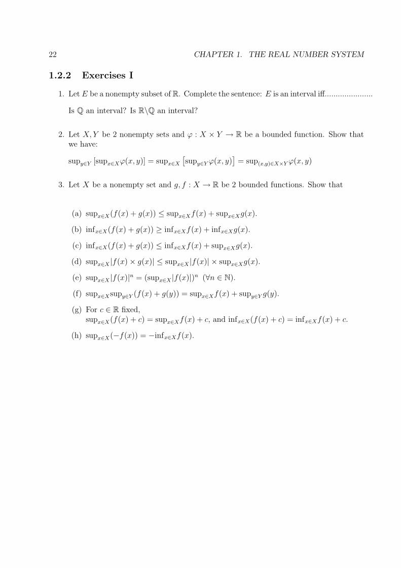
1.2.2 Exercises I
1. Let E be a nonempty subset of R. Complete the sentence: E is an interval iff......................
Is Q an interval? Is R\Q an interval?
2. Let X,Y be 2 nonempty sets and ϕ : X × Y → R be a bounded function. Show thatwe have:
supy∈Y [supx∈Xϕ(x, y)] = supx∈X
[supy∈Y ϕ(x, y)
]= sup(x,y)∈X×Y ϕ(x, y)
3. Let X be a nonempty set and g, f : X → R be 2 bounded functions. Show that
(a) supx∈X(f(x) + g(x)) ≤ supx∈Xf(x) + supx∈Xg(x).
(b) infx∈X(f(x) + g(x)) ≥ infx∈Xf(x) + infx∈Xg(x).
(c) infx∈X(f(x) + g(x)) ≤ infx∈Xf(x) + supx∈Xg(x).
(d) supx∈X |f(x) × g(x)| ≤ supx∈X |f(x)| × supx∈Xg(x).
(e) supx∈X |f(x)|n = (supx∈X |f(x)|)n (∀n ∈ N).
(f) supx∈Xsupy∈Y (f(x) + g(y)) = supx∈Xf(x) + supy∈Y g(y).
(g) For c ∈ R fixed,supx∈X(f(x) + c) = supx∈Xf(x) + c, and infx∈X(f(x) + c) = infx∈Xf(x) + c.
(h) supx∈X(−f(x)) = −infx∈Xf(x).

1.3. CONVERGENCE IN R AND MONOTONE SEQUENCES 23
1.3 Convergence in R and Monotone Sequences
Definition 1.3.1 Let (xn)n∈N be a sequence in R.
• (xn)n∈N is convergent if there is a number L that satisfies the condition:
∀ε > 0,∃ N ∈ N, ∀n > N =⇒ |xn − L| < ε
Equivalently, ∀ε > 0, xn ∈ ]L − ε, L + ε[ for all but finitely many n ∈ N
• In this case we write, xn → L, as n → ∞, L = limn→∞xn
• If (xn)n∈N does not converge to any L ∈ R, then we say that (xn)n∈N diverges.
Example 1.3.2 Let xn = (−1)n. There is no L ∈ R that satisfies the condition of con-vergence. Indeed, if it was convergent there would be an L ∈ R satisfying the convergence
condition. Now let ε =1
2. Then for N corresponding to this ε, ∀n ≥ N, |xn − L| <
1
2.
Now for n odd ⇒ xn = −1 and |−1 − L| <1
2
for n even ⇒ xn = 1 and |1 − L| <1
2
So we have−1
2< 1 + L <
1
2and
−1
2< 1 − L <
1
2, and adding these we get −1 < 2 < 1
which is nonsense. Hence xn is divergent (does not mean that it goes to infinity.) as,|xn| = 1 ∀ n ∈ N.
Example 1.3.3 Let xn = n2 + 1. If it is convergent to some L ∈ R then,∀ ε > 0, ∃N ∈ N, ∀n > N, |n2 + 1 − L| < ε. i.e. L − ε < n2 + 1 < L + ε ∀, n ∈ N.But this is not possible, since N is not bounded from above.
Example 1.3.4 (xn)n∈N =
{0, 1,
1
2, 3,
1
4, ...
}. This sequence does not converge either.
Example 1.3.5 Let xn =1
n, then the Archimedian property just means that
1
n→ 0, as
n → ∞.(∀ ε > 0 ∃ N ∈ N
1
N< ε =⇒ ∀n ≥ N,
1
n< ε =⇒ 1
n→ 0
)
Theorem 1.3.6 Properties of the Convergent Sequences:
1. Uniqueness of the Limit: A sequence (xn)n∈N cannot converge to more than onelimit.

24 CHAPTER 1. THE REAL NUMBER SYSTEM
2. Boundaries of Convergent Sequences: Every convergent sequence (xn)n∈N in Ris bounded.
3. Passage to Absolute Value: If xn → L, then |xn| → |L|.4. Convergence and Inequalities: If xn ≥ c, ∀n ∈ N and xn → L, then L ≥ c.
5. If xn ≤ yn ∀n ∈ N, xn → L, yn → S, then L ≤ S.
6. Sandwich Theorem: xn ≤ yn ≤ zn for all n ∈ N, and xn → L, zn → L, thenyn → L.
7. If xn → L, and L �= 0, then |xn| ≥ |L|2
for all but finitely many n ∈ N.
8. If xn → L and yn → S, then
(a) xn+ yn → L + S
(b) xn × yn → L × S
(c) If S �= 0,xn
yn
→ L
S
Proof 1.3.7 1. For a contradiction, suppose that xn → S and xn → L, (L �= S). SayL < S. Let ε be small enough to have ]L − ε, L + ε] ∩ ]S − ε, S + ε[ = ∅. So,
0 < ε <S − L
3. Since xn → L , xn ∈ ]L − ε, L + ε[ for all but finitely many n. As
xn → S , xn ∈ ]S − ε, S + ε[ for all but finitely many n, too. This is not possible.Hence the limit is unique.
2. Let, xn → L, as n → ∞. So, we have: ∀ε > 0, ∃N ∈ N,∀n ≥ N, |xn − L| < ε.
Hence, since ||xn| − |L|| ≤ |xn − L| < ε, ∀n ≥ N |xn| ≤ |L| + ε.
Let M = max {|x0| , |x1| , ..., |xn| , |L| + ε}. Then ∀n ∈ N |xn| ≤ M .
Remark: Converse of this result is false. Let xn = (−1)n. Then |xn| ≤ 1 ∀n ∈ N,but (xn)n∈N does not converge.
3. As xn → L, we have ∀ε > 0 ∃N ∈ N, ∀n ≥ N |xn − L| < ε. As ||xn| − |L|| ≤|xn − L|, we see that ∀n ≥ N ||xn| − |L|| < ε. This means that |xn| → |L|.
4. For a contradiction, suppose that L < c. Let ε be small enough to have L + ε < c.
(e.g. let ε =c − L
2). Write the definition of convergence for this ε. Then, there is
N ∈ N ∀n ≥ N, |xn − L| < ε. So, L − ε ≤ xn ≤ L + ε. As xn ≥ c, and L + ε < c.Contradiction.
In particular, if xn ≥ 0 ∀n ∈ N, then L ≥ 0.
Remark:

1.3. CONVERGENCE IN R AND MONOTONE SEQUENCES 25
• If xn > c and xn → L, we can not say L > c, all we can say is L ≥ c. e.g. Let
xn =1
n, then xn > 0∀n ≥ 1, but limn→∞xn = 0.
• If L ≥ c, we can not say that xn ≥ c for all n ∈ N.
5. For a contradiction, suppose L > S. Let ε > 0 be small enough to still have L − ε >S + ε. For this ε > 0, we write the fact that xn → L, yn → S. Then, there isN1 ∈ N, ∀n ≥ N1, |xn − L| < ε. Then, there is N2 ∈ N, ∀n ≥ N2, |xn − S| < ε.
Let N = max {N1, N2}. So ∀n ≥ N, L − ε ≤ xn ≤ L + ε, and S − ε ≤ yn ≤ S + ε.As S < L − ε < xn ≤ yn < S + ε < L − ε is not possible, this is contradiction.
6. Let ε > 0, then xn → L, zn → L.∃N ∈ N ∀n ≥ N L − ε ≤ xn ≤ L + ε
L − ε ≤ zn ≤ L + ε
∀n ≥ N, L − ε < xn ≤ yn ≤ zn < L + ε.
So, ∀n ≥ N, L − ε < yn < L + ε =⇒ |yn − L| < ε. Then, yn → L.
7. Let ε =|L|2
. So ε > 0.
Corresponding to this ε there is an N ∈ N such that ∀n ≥ N, |xn − L| < ε.
As ||xn| − |L|| ≤ |xn − L| < ε, we have
|L| − ε︸ ︷︷ ︸ < |xn| < |L| + ε
=|L|2
=⇒ ∀n ≥ N, |xn| ≥ |L|2
8. (a)∀ε > 0∃N ∈ N ∀n ≥ N, |xn − L| <
ε
2∀ε > 0∃N ∈ N, ∀n ≥ N |yn − S| <
ε
2Then, ∀n ≥ N, |xn + yn − (S + L)| ≤ |xn − L| + |yn − S| < ε.
Hence, xn + yn → S + L
(b) xn × yn − L × S = (xn − L) × yn + L × yn − L × S.
Hence, |xn × yn − L × S| ≤ |xn − L| × |yn| + |L| × |yn − S|As (yn)n∈N converges, it is bounded, say |yn| ≤ M ∀n ∈ N
Then, n ≥ N, |xn × yn − L × S| < Mε
2+ |L| ε
2≤ M + |L|2.
Hence, xn × yn → L × S.
(c)xn
yn
− L
S=
xnS − ynL
ynS
Since S �= 0, by ref2.3.7 |yn| ≥ |S|2
for all but finitely many n ∈ N. Then,

26 CHAPTER 1. THE REAL NUMBER SYSTEM
∣∣∣∣xnS − ynL
ynS
∣∣∣∣ ≤ 2
∣∣∣∣xnS − ynL
|S|2∣∣∣∣→ 2
∣∣∣∣SL − SL
|S|2∣∣∣∣ = 0.
Hence,
∣∣∣∣xn
yn
− L
S
∣∣∣∣→ 0,xn
yn
→ L
S.
1.4 Monotone Sequences
Definition 1.4.1 A sequence (xn)n∈N in R is said to be
1. increasing if x0 ≤ x1 ≤ ... ≤ xn ≤ ...
2. decreasing if x0 ≥ x1 ≥ ... ≥ xn ≥ ...
e.g. xn =1
nis decreasing,
xn =n
n + 1is increasing
Remark:
• Any increasing sequence is bounded from below.
• Any decreasing sequence is bounded from above.
So an increasing sequence is bounded iff it is bounded from above.
• Also, (xn)n∈N is increasing iff (−xn) is decreasing.
Example 1.4.2 Let xn = 1 +1
2!+ · · · + 1
n!. Then, clearly, xn is increasing.
3! ≥ 22. Hence,1
3!≥ 1
22
4! ≥ 23. Hence1
4!≥ 1
23
5! ≥ 24. Hence1
5!≥ 1
24
...
n! ≥ 2n. Hence1
n!≥ 1
2n−1.
Hence, xn ≤ 5
2+
1
22+
1
23+
1
24+ · · · + 1
2n−1︸ ︷︷ ︸=
1
22
[1 +
1
2+
1
22+
1
23+
1
24+ · · · + 1
2n−3
]
=1
22
1 − (1
2)n−2
1 − 1
2
≤ 1
2
So, xn ≤ 5
2+
1
2=⇒ xn ≤ 3, ∀n ∈ N =⇒ xn is bounded.

1.4. MONOTONE SEQUENCES 27
Example 1.4.3 Let xn = 1 +1
2!+ · · · + 1
n!and yn = xn +
1
n!.
So, yn−1 − yn = xn−1 − xn +1
(n − 1)!− 1
n!= − 2
n!+
1
(n − 1)!=
n − 2
n!≥ 0, ∀n ≥ 2.
Hence, yn−1 ≥ yn. So, (yn)n∈N is decreasing.
Example 1.4.4 1 +1
22+
1
32+ · · · + 1
n2. Then, x1 ≤ x2 ≤ ... ≤ x3 ≤ ...
As n2 ≥ n(n − 1),1
n2≤ 1
n(n − 1)=
1
n − 1− 1
n
i.e.1
22≤ 1
1− 1
21
32≤ 1
2− 1
3...1
n2≤ 1
n − 1− 1
n
Then, xn ≤ 2 − 1
n≤ 2, ∀n ≥ 1, xn ≤ 2.
Theorem 1.4.5 (Convergence of monotone sequences): A monotone sequence (xn)n∈N
is convergent iff it is bounded. In this case,
1. if xn is increasing, then limn→∞xn = sup {x0, x1, x2, . . . , xn, . . .}2. if xn is decreasing, then limn→∞xn = inf {x0, x1, x2, . . . , xn, . . .}
Proof 1.4.6 Suppose x0 ≤ x1 ≤ x2 ≤ . . . ≤ xn ≤ . . .We know that every convergent sequence is bounded.Conversely, suppose that (xn)n∈N is bounded. Then the set A = {x0, x1, x2, ..., xn, . . .} is
bounded. So by the supremum axiom, ∃α ∈ R, α = sup A
=⇒{
1) ∀n ∈ N, xn ≤ α2) ∀ε ≥ 0, ∃ xN ∈ A xN > α − ε
ε > 0 being given. For every n ≥ N α − ε < xN ≤ xn ≤ α ≤ α + ε.So, ∀n ∈ N, |xn − α| < ε, i.e. limn→∞xn = α
Example 1.4.7 1. Let xn = 1 +1
1+
1
2+ · · · + 1
n. We have seen that xn is not bounded.
So it diverges by the theorem 1.4.5.
2. Let xn = 1 +1
1!+
1
2!+ · · · + 1
n!. We have seen that xn ≤ 3 ∀n ∈ N. This sequence is
increasing, so it converges.
Let e = limn→∞xn. Since xn ≤ 3 ∀n ∈ N, e ≤ 3.
As x2 = 2.5, we see that 2.5 ≤ e ≤ 3.

28 CHAPTER 1. THE REAL NUMBER SYSTEM
Remark: If the sequence (xn)n∈N is strictly increasing, i.e. x0 < x1 < x2 < . . . < xn < . . .and L is the limit, then xn ≤ L, ∀n ∈ N. Hence xn < e in above example.
Now, let yn = xn +1
n!. This sequence is decreasing and bounded from below by 0. So, it
converges. Hence, yn − xn =1
n!→ 0 also converges. limn→∞yn = e.
Theorem 1.4.8 The number e is not rational.
Proof 1.4.9 Let as in the last example, xn = 1 +1
1!+
1
2!+ · · ·+ 1
n!and yn = 1 +
1
1!+
1
2!+
· · · + 1
n!+
1
n!. Then, for any n ∈ N xn < e < yn.
For a contradiction, suppose e is rational. So, e =p
q, (p > 0, q > 0, p, q ∈ N)
Let n ≥ q, 1 +1
1!+
1
2!+ · · · + 1
n!<
p
q< 1 +
1
1!+
1
2!+ · · · + 1
n!+
1
n!.
Multiplying by n!; n! +n!
1!+
n!
2!+ · · · + 1 <
pn!
q< n! +
n!
1!+
n!
2!+ · · · + 1 + 1
n! +n!
1!+
n!
2!+ · · · + 1 = N
n! +n!
1!+
n!
2!+ · · · + 1 + 1 = N + 1, and
pn!
q= M
N < M < N + 1. Hence, N and M are integers. As there is no integer between twoconsecutive integers, this is not possible.
Hence e is not rational
This theorem says that Q is not closed under the “limit” operation. Indeed, althoughevery xn ∈ Q, lim xn = e /∈ Q.
1.4. MONOTONE SEQUENCES 29
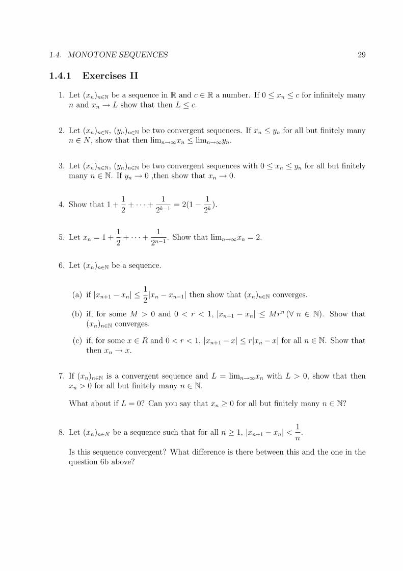
1.4.1 Exercises II
1. Let (xn)n∈N be a sequence in R and c ∈ R a number. If 0 ≤ xn ≤ c for infinitely manyn and xn → L show that then L ≤ c.
2. Let (xn)n∈N, (yn)n∈N be two convergent sequences. If xn ≤ yn for all but finitely manyn ∈ N , show that then limn→∞xn ≤ limn→∞yn.
3. Let (xn)n∈N, (yn)n∈N be two convergent sequences with 0 ≤ xn ≤ yn for all but finitelymany n ∈ N. If yn → 0 ,then show that xn → 0.
4. Show that 1 +1
2+ · · · + 1
2k−1= 2(1 − 1
2k).
5. Let xn = 1 +1
2+ · · · + 1
2n−1. Show that limn→∞xn = 2.
6. Let (xn)n∈N be a sequence.
(a) if |xn+1 − xn| ≤ 1
2|xn − xn−1| then show that (xn)n∈N converges.
(b) if, for some M > 0 and 0 < r < 1, |xn+1 − xn| ≤ Mrn (∀ n ∈ N). Show that(xn)n∈N converges.
(c) if, for some x ∈ R and 0 < r < 1, |xn+1 − x| ≤ r|xn − x| for all n ∈ N. Show thatthen xn → x.
7. If (xn)n∈N is a convergent sequence and L = limn→∞xn with L > 0, show that thenxn > 0 for all but finitely many n ∈ N.
What about if L = 0? Can you say that xn ≥ 0 for all but finitely many n ∈ N?
8. Let (xn)n∈N be a sequence such that for all n ≥ 1, |xn+1 − xn| <1
n.
Is this sequence convergent? What difference is there between this and the one in thequestion 6b above?
30 CHAPTER 1. THE REAL NUMBER SYSTEM
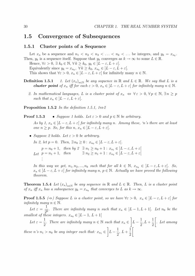
1.5 Convergence of Subsequences
1.5.1 Cluster points of a Sequence
Let xn be a sequence and n1 < n2 < n3 < . . . < nk < . . . be integers, and yk = xnk.
Then, yk is a sequence itself. Suppose that yk converges as k → ∞ to some L ∈ R.Hence, ∀ε > 0, ∃ k0 ∈ N, ∀ k ≥ k0, yk ∈ ]L − ε, L + ε[.Equivalently since yk = xnk
, ∀ k ≥ k0, xnk∈ ]L − ε, L + ε[.
This shows that ∀ε > 0, xn ∈ ]L − ε, L + ε[ for infinitely many n ∈ N.
Definition 1.5.1 1. Let (xn)n∈N be any sequence in R and L ∈ R. We say that L is acluster point of xn iff for each ε > 0, xn ∈ ]L − ε, L + ε[ for infinitely many n ∈ N.
2. In mathematical languages, L is a cluster point of xn ⇔ ∀ ε > 0, ∀ p ∈ N, ∃n ≥ psuch that xn ∈ ]L − ε, L + ε[.
Proposition 1.5.2 In the definition 1.5.1, 1⇔2
Proof 1.5.3 • Suppose 1 holds. Let ε > 0 and p ∈ N be arbitrary.
As by 1, xn ∈ ]L − ε, L + ε[ for infinitely many n. Among these, ‘n’s there are at leastone n ≥ p. So, for this n, xn ∈ ]L − ε, L + ε[.
• Suppose 2 holds. Let ε > 0 be arbitrary.
In 2, let p = 0. Then, ∃n0 ≥ 0 : xn0 ∈ ]L − ε, L + ε[.
Let
p = n0 + 1, then by 2 ∃ n1 ≥ n0 + 1 : xn1 ∈ ]L − ε, L + ε[p = n1 + 1, then ∃ n2 ≥ n1 + 1 : xn2 ∈ ]L − ε, L + ε[...
In this way we get, n1, n2, ..., nk such that for all k ∈ N, xnk∈ ]L − ε, L + ε[. So,
xn ∈ ]L − ε, L + ε[ for infinitely many n, p ∈ N. Actually we have proved the followingtheorem.
Theorem 1.5.4 Let (xn)n∈N be any sequence in R and L ∈ R. Then, L is a cluster pointof xn iff xn has a subsequence yk = xnk
that converges to L as k → ∞.
Proof 1.5.5 (⇒) Suppose L is a cluster point, so we have ∀ε > 0, xn ∈ ]L − ε, L + ε[ forinfinitely many n ∈ N.
Let ε =1
20. There are infinitely many n such that xn ∈ ]L − 1, L + 1[. Let n0 be the
smallest of these integers. xn0 ∈ ]L − 1, L + 1[
Let ε =1
2. There are infinitely many n ∈ N such that xn ∈
]L − 1
2, L +
1
2
[. Let among
these n’s n1 > n0 be any integer such that: xn1 ∈]L − 1
2, L +
1
2
[

1.5. CONVERGENCE OF SUBSEQUENCES 31
Next, let ε =1
22. There are infinitely many n such that xn ∈
]L − 1
4, L +
1
4
[.
Let among these n’s n2 > n1 be any integer. So, xn2 ∈]L − 1
4, L +
1
4
[.
Let ε =1
23
...In this way we construct a sequence of integers n0 < n1 < n2 < . . . < nk < ... such that,
∀k ∈ N, xnk∈]L − 1
2k, L +
1
2k
[.
Hence, |xnk− L| <
1
2k. As k → ∞, xnk
→ L.
(⇐) Suppose that xn has a subsequence ynkthat converges to L as k → ∞.
So ∀ε > 0,∃ k0 ∈ N, ∀ k ≥ k0, yk ∈ ]L − ε, L + ε[. Hence, as we have seen above, thismeans ∀ε > 0, xn ∈ ]L − ε, L + ε[ for infinitely many n ∈ N. So, L is a cluster point.
Example 1.5.6 Let xn = (−1)n. This sequence is not convergent, but it has convergentsubsequences. Indeed, L = 1 and L = −1 are cluster points.
Let L = 1. Then, ∀ε > 0, x2n ∈ ]1 − ε, 1 + ε[ for all n ∈ N. So, L = 1 is a cluster point.
Example 1.5.7 (xn)n∈N = 0, 1,1
2, 3,
1
4, 5,
1
6, 7, ...
Here L = 1 is a cluster point of this sequence. Indeed the subsequence
(1
2,1
4,1
6, · · · ,
1
2n, · · · ) → 0
Example 1.5.8 Let xn = 1, 2, 3, 4, 1, 2, 3, 4, 1, 2, 3, 4, .... Then, 1, 2, 3, 4 are cluster points.
Example 1.5.9 Let [0, 1] ∩ Q = {x0, x1, ..., xn, ...} in any order. Consider the sequence(xn)n∈N. ∀L ∈ [0, 1] , ∀ε > 0, the interval ]L − ε, L + ε[ contains infinitely many rationalnumbers. So, xn ∈ ]L − ε, L + ε[ for infinitely many n. Hence, any L ∈ [0, 1] is a clusterpoint of (xn)n∈N.
Example 1.5.10 xn = en, ∀n ∈ N. xn has no cluster points.
Theorem 1.5.11 Let xn be a sequence in R. xn → L iff L is the only cluster point of xn.
Proof 1.5.12 (=⇒) If xn → L, then every subsequence of xn converges to the same L. So,x2n → L and x2n+1 → L
(⇐=) Suppose that x2n → L and x2n+1 → L. So, we have:∀ε > 0, ∃ N1 ∈ N : ∀n ≥ N |x2n − L| < ε.∀ε > 0, ∃ N2 ∈ N ∀n ≥ N |x2n+1 − L| < εLet, N ′ = max {N1, N2} and N = 2N ′ + 1. Then n ≥ N |xn − L| < ε =⇒ xn → L

32 CHAPTER 1. THE REAL NUMBER SYSTEM
Lemma 1.5.13 Bolzano-Weierstrass Theorem: Every sequence (xn)n∈R has a mono-tone subsequence.
Proof 1.5.14 Let
F0 = {x0, x1, ..., xn, ...}F1 = {x1, x2, ..., xn, ...}...Fn = {xn, xn+1, ...}
Clearly, F0 ⊇ F1 ⊇ F2 ⊇ . . . ⊇ Fn ⊇ . . .
There are two possibilities:
1. Every Fn has a smallest element.
2. There is p ∈ N, such that Fp does not have a smallest element.
• Suppose 1 holds: So, every Fn has a smallest element. Let xn0 be the smallest elementof F0. Then consider the set Fn0+1. Then Fn0+1 has a smallest element call it xn1.Obviously, n1 > n0 and xn0 ≤ xn1, since F0 ⊆ Fn0+1. Next, let consider the setFn1+1. Then Fn1+1 has a smallest element call it xn2. So n2 > n1 and xn1 ≤ xn2.Next, let consider the set Fn2+1, it has a smallest element call it xn3 , ... so on. Then,n0 < n1 < n2 < ... < nk < ... and xn0 ≤ xn1 ≤ xn2 ≤ . . . ≤ xnk
≤ . . .. So, (xnk)k∈N
isan increasing subsequence of the initial subsequence.
• Suppose 2 holds: So, for some p ∈ N, Fp has no smallest element. But then, for anyn ≥ p, Fp = {xp+1,...,xn−1} ∪ Fn. Fn can not have a smallest element either. Hence,∀n ≥ p, Fn has no smallest element.
Let xn0 be any element in Fp. Consider Fn0+1. Fn0+1 has no smallest element. So,there is an element call it xn1 ∈ Fn0+1 xn1 < xn0 (Clearly n1 > n0). Now considerFn1+1, it has no smallest element. So, there is an element call it xn2 ∈ Fn1+1 xn2 <xn1. Consider Fn2+1, . . . and so on. In this way, we get xn0 > xn1 > xn2 > . . . andn0 < n1 < n2 < . . . < nk < . . . So, (xnk
)k∈Nis a decreasing subsequence of (xn)n∈N.
Theorem 1.5.15 (Fundamental Theorem of Real Analysis) Every bounded sequence(xn)n∈N in R has at least one convergent subsequence. (Or equivalently at least one clusterpoint.)
Proof 1.5.16 By the lemma 1.5.13, xn has a monotone subsequence. Since every boundedmonotone sequence converges, we conclude that xn has a convergent subsequence.
Let xn = sin n. Then xn has a convergent subsequence.

1.5. CONVERGENCE OF SUBSEQUENCES 33
1.5.2 Cauchy Sequences
Let xn∈N be a sequence. Suppose we only know that, |xn+1 − xn| =1
2n. Does such a sequence
converge? Let xn = 1 +1
2+ · · · + 1
n. Then, |xn+1 − xn| =
1
n + 1. So, |xn+1 − xn| → 0. But
(xn)n∈N diverges.
Let xn = 1 +1
22+
1
32+ · · · +
1
n2. Then |xn+1 − xn| =
1
(n + 1)2→ 0. This time as we
know (xn)n∈N converges. Now let xn be a sequence that converges to some L ∈ R. So wehave:
∀ ε > 0, ∃N ∈ N∀n ≥ N |xn − L| <ε
2Hence,∀n ≥ N, ∀m ≥ N ,
|xn − xm| = |xn − L + L − xm| ≤ |xn − L|︸ ︷︷ ︸ + |xm − L|︸ ︷︷ ︸ < ε
<ε
2<
ε
2i.e., if xn converges, we have:
∀ε > 0, ∃n ∈ N, ∀n ≥ N, ∀m ≥ N, |xn − xm| < ε
This is a necessary condition for convergence.
Definition 1.5.17 A sequence in R is said to be a Cauchy sequence if it satisfies theCauchy condition, that is:
∀ε > 0, ∃N ∈ N ∀n ≥ N, ∀m ≥ N |xn − xm| < ε
n and m are independent from each other.
This condition is equivalent to :
∀ε > 0, ∃N ∈ N ∀n ≥ N ∀ p ∈ N |xn+p − xn| < ε.
Again it is equivalent to limn→∞, m→∞ |xn − xm| = 0
Example 1.5.18 Prove or disprove that the following sequences are Cauchy sequences.
1. xn = 1 +1
2+ · · · + 1
n
2. xn = 1 +1
2+ · · · + 1
2n
3. |xn+1 − xn| ≤ 1
2n
1. x2n − xn =1
n + 1+ · · · + 1
2n≥ 1
2n=
1
2
|x2n − xn| ≥ 1
2. Let ε =
1
4. Contradiction. Then the sequence is not Cauchy.

34 CHAPTER 1. THE REAL NUMBER SYSTEM
2. |xn+p − xn| =1
2n+1+· · ·+ 1
2n+p=
1
2n+1
(1 +
1
2+ · · · + 1
2p−1
)=
1
2n+1
⎛⎜⎜⎝
1 −(
1
2
)p
1 − 12
⎞⎟⎟⎠ ≤
1
2n.
∀n ≥ 0, ∀ p ≥ 0, |xn+p − xn| ≤ 1
2n.
1
2n→ 0. So, ∀ε > 0, ∃N ∈ N ∀n ≥ N,
1
2n< ε.
Hence, ∀n ≥ N, ∀ p ∈ N, |xn+p − xn| < ε, so (xn)n∈N is Cauchy.
3. Our sequence (xn)n∈N satisfies the condition |xn+1 − xn| ≤ 1
2n.
Hence,
|xn+p − xn| = |xn+p + xn+p−1 − xn+p−1 + xn+p−2 − xn+p−2 − xn|≤ |xn+p − xn+p−1| + |xn+p−1 − xn+p−2| + . . . + |xn+1 − xn|≤ 1
2n+p−1+
1
2n+p−2+ · · · + 1
2n
Since |xn+p − xn+p−1| ≤ 1
2n+p−1, |xn+p−1 − xn+p−2| ≤ 1
2n+p−2, |xn+1 − xn| ≤ 1
2n.
As1
2n→ 0, ∀ ε > 0, ∃N ∈ N, ∀n ≥ N
1
2n< ε. So ∀n ≥ N, ∀ p ∈ N, |xn+p − xn| < ε.
Hence, (xn)n∈N is Cauchy.
Note: Concerning any sequence (xn)n∈N, there are two basic questions:
1. Does (xn)n∈N converge?
2. If it does, what is limn→∞xn?
Proposition 1.5.19 Every Cauchy sequence (xn)n∈N in R is bounded.
Proof 1.5.20 As xn is Cauchy, we have ∀ε > 0, ∃N ∈ N ∀n,m ≥ N, |xn − xm| < ε. Fixm = N . Then, |xn| = |xn − xN + xN | ≤ ε + |xN | ∀n ≥ N . Hence, sup {|xn| : n ∈ N} ≤sup {|x0| , . . . , |xN | : ε + |xN |}. So, xn is bounded.
Theorem 1.5.21 (R is complete): A sequence xn in R is convergent iff it is Cauchy.
Proof 1.5.22 We have already seen that every convergent sequence is Cauchy.Conversely, assume xn is Cauchy. So it is bounded. Hence, by Bolzano Weierstrass
Theorem xn has a convergent subsequence, yk = xnk.
Let limk→∞yk = L. Let us see not only xnk, but the whole sequence converges to L.
Indeed yk → L means that:

1.5. CONVERGENCE OF SUBSEQUENCES 35
∀ ε > 0, ∃ k0 ∈ N ∀ k ≥ k0 |xnk− L| <
ε
2*
As xn is Cauchy, we also have: ∀ε > 0, ∃N ∈ N ∀n,m ≥ N |xn − xm| <ε
2.
Let k ≥ k0 be such that nk ≥ N .
Then ∀n ≥ N ,
|xn − L| = |xn − xnk+ xnk
− L| ≤ |xn − xnk|︸ ︷︷ ︸ + |xnk
− L|︸ ︷︷ ︸ ≤ ε
≤ ε
2(by Cauchy) ≤ ε
2(by * )
Hence xn → L.

36 CHAPTER 1. THE REAL NUMBER SYSTEM
1.5.3 Exercises III
1. Let (xn)n∈N be a sequence in R. Show that xn → x iff there exists a decreasing sequence(tk)k∈N, tk ≥ 0, tk → 0 such that |xn − x| ≤ tn for n large.
2. Let (xn)n∈N and (yn)n∈N be two convergent sequences with limn→∞xn = a = limn→∞yn.Consider the ”mixed sequence” zn : x0, y0, x1, y1, x2, y2, . . . Show that zn → a too.
3. Show that given any x in R there exists a sequence of rational numbers (rn)n∈N anda sequence of irrational numbers (sn)n∈N such that rn → x and sn → x.
4. Let (xn)n∈N be a sequence in R. Assume xn ∈ Z for each n ∈ N. Show that (xn)n∈N isconvergent iff (xn)n∈N is almost constant i.e. ∃ N ∈ N, ∀n ≥ N, ∀m ≥ N, xn = xm.
5. Let (xn)n∈N be a positive sequence. If xn → 0 show that then xn
1+xn→ 0 too.
Conversely, if xn
1+xn→ 0 show that then xn → 0 too.
6. Let xn = ln(n + 1). Show that |xn+1 − xn| → 0 as n → ∞.
Is (xn)n∈N Cauchy? Is (xn)n∈N convergent?
7. For 0 ≤ b ≤ a, find limk→∞(ak + bk)1k .
8. If xn > c for all n ∈ N and xn → x, can you say that x > c?

1.6. LIM SUP, LIM INF 37
1.6 lim sup, lim inf
Let (xn)n∈N be a bounded sequence. Say a ≤ xn ≤ b (∀n ∈ N). Bolzano Weierstrass’Theorem says that xn has at least one cluster point, say L. Then, a ≤ L ≤ b. We alsoknow that xn may have uncountably many cluster points. Let F be the set of all the clusterpoints. F �= ∅ and F ⊆ [a, b].
We are going to show that F has a smallest element which we call lim inf xn, and a largestelement which we call lim sup xn. Next, we are going to prove the existence of these clusterpoints.
Let F0 = {x0, x1, x2, . . . , xn}F1 = {x1, x2, x3, . . . , xn}F2 = {x2, x3, x4, . . . , xn}...Fn = {xn, xn+1, . . .}
F0 ⊇ F1 ⊇ F2 ⊇ . . . ⊇ Fn ⊇ . . . and Fn ⊆ [a, b] (∀n ∈ N).By the supremum axiom, sup Fn and inf Fn exist. Let yn = inf Fn, zn = sup Fn. Since
F1 ⊇ F2 ⊇ . . . ⊇ Fn ⊇ . . . , y0 ≤ y1 ≤ . . . ≤ yn ≤ . . . ≤ b and z0 ≥ z1 ≥ . . . ≥ zn ≥ . . . ≥ a.Hence we have two monotone bounded sequences: yn, zn.Hence l = limn→∞yn and L = limn→∞zn exists.Moreover, l = supn∈Nyn and L = infn∈Nzn. As yn = infk≥nxk, and zn = supk≥nxk, so that
l = supn∈N infk≥nxk and L = infn∈N supk≥nxk
Example 1.6.1 Let xn = (−1)n. Then Fn = {xn, xn+1, . . .} = {−1, 1} , ∀n ∈ N.Hence, yn = −1, zn = 1. So, yn → −1, and zn → 1.Hence, lim sup xn = 1, lim inf xn = −1.
Example 1.6.2 Let xn = 0, 1, 2, 3, 4, 0, 1, 2, 3, 4, 0, 1, 2, 3, 4, . . .. Then ∀n ≥ 0, Fn = {0, 1, 2, 3, 4}.Then yn = 0, zn = 4. Hence, lim sup xn = 4, lim inf xn = 0.
Theorem 1.6.3 Let xn be a bounded sequence: l = limn→∞infn∈N xn, L = limn→∞supn∈Nxn.Then
1. l and L are cluster points of xn.
2. l is the smallest cluster point and L is the largest cluster point of xn.
Proof 1.6.4 First observe that limn→∞supn∈N (−xn) = −limn→∞infn∈Nxn. Hence, it isenough to prove the theorem for L.
To show that L is a cluster point, we have to show that given:1 ∀ε > 0, xn ∈ ]L − ε, L + ε[ for infinitely many n ∈ N.Let ε > 0 be given. Since zn → L, by the definition of the convergence,∃N ∈ N ∀n ≥ N |zk − L| < ε. As zk = inf {xk, xk+1, . . .}, we conclude that:2 ∀k ≥ N, ∃nk ≥ k : xnn ∈ ]L − ε, L + ε[

38 CHAPTER 1. THE REAL NUMBER SYSTEM
1 ⇔ 2 So, L is a cluster point.Let us see that L is the largest of the all cluster points of xn.If not, for some cluster point S of xn you would have S > L. Let ε > 0 be such that
]S − ε, S + ε[ ∩ ]L − ε, L + ε[ = ∅. As S is a cluster point xn ∈ ]S − ε, S + ε[ for infinitelymany n ∈ N. In particular, zn = sup {xn, xn+1, . . .} ≥ L + ε ∀n ∈ N. As zn → L, this is notpossible. So L is the largest cluster point of xn.
Main interest of lim sup, lim inf is that they always exist whereas limn→∞xn exists onlyexceptionally.
Theorem 1.6.5 Let (xn)n∈N be a bounded sequence. Then, xn converges ifflimn→∞supn∈Nxn = limn→∞infn∈Nxn
Proof 1.6.6 If xn → L, then L is the only cluster point of xn.So limn→∞supn∈N = limn→∞infn∈N = L.Conversely, if lim sup = lim inf, then this implies that xn has only one cluster point,
namely S = lim sup = lim inf.To finish the proof it is enough to prove the following result.
Proposition 1.6.7 If xn is bounded and has only one cluster point, (L) then, xn → L.
Proof 1.6.8 If xn does not converges to L then, ∃ε > 0 xn /∈ ]L − ε, L + ε[ for infinitelymany n ∈ N. Suppose xn ≥ L+ε for infinitely many n ∈ N : n0 < n1 < n2 < . . . < nk < . . .
So that ,yk ≥ L + ε, where yk = xnk.
yk is a subsequence of xn. As xn is bounded so is yk. Hence by the Bolzano Weierstrass’theorem yk has a convergent subsequence. ykp → S, and since yk ≥ L + ε, in particular,S �= L but as S is also a cluster point of xn we have contradiction. So, xn → L.
Remark: If xn is not bounded, the preceding lemma is false.
Example 1.6.9 Let xn = 1, 12, 3, 1
4, 5, 1
6, . . . Then, 0 is the only cluster point of xn. But xn
does not converges to 0. Hence, a sequence xn diverges iff xn is unbounded (for example:xn = en) or xn is bounded but has more than one cluster points.(for example: xn = (−1)n)
Theorem 1.6.10 Let xn and yn be two bounded sequences.
1. lim sup (xn + yn) ≤ lim sup xn + lim sup yn
2. lim inf (xn + yn) ≥ lim inf xn + lim inf yn
3. If xn ≥ 0 and yn ≥ 0, then lim sup (xnyn) ≤ lim sup xn × lim sup yn
4. If xn or yn converges, then the above inequalities become equality.
Proof 1.6.11 Let An = {xn, xn+1, . . .}, Bn = {yn, yn+1, . . .}, Cn = {xn + yn, xn+1 + yn+1, . . .}.Then,

1.7. ELEMENTARY TOPOLOGY OF R 39
1. sup Cn ≤ sup An + sup Bn
Let X = {n, n + 1, . . .} , f : X → R, f(n) = xn, g : X → R, g(n) = yn. Hence,passing to limits, lim sup(xn + yn) ≤ lim sup xn + lim sup yn
2. infCn ≥ inf An + inf Bn. Similarly, lim sup(xnyn) ≤ lim sup xn × yn
3. As xn, yn > 0, xn×yn > 0, so sup(xn×yn) ≤ sup xn×sup yn. Hence, passing to limits,lim sup (xnyn) ≤ lim sup xn × lim sup yn
4. Suppose xn → L.
• Let S = lim sup yn. Since S is a cluster point of yn, ∃ a subsequence
ynk→ S. Then, since xn → L, xnk
→ L too.
xnk+ ynk
→ L + S. Hence, L + S is a cluster point of xn + yn
Since lim sup(xn + yn) ≤ lim sup xn + lim sup yn = L + S
Hence L + S = lim sup(xn + yn)
• Similarly, let s = lim inf yn. Since s is a cluster point of yn, ∃ a subsequence
ynk→ s. Then, since xn → L, xnk
→ L too.
xnk+ ynk
→ L + s. Hence, L + s is a cluster point of xn + yn
Since lim inf(xn + yn) ≥ lim inf xn + lim inf yn = L + s
Hence L + s = lim inf(xn + yn)
• As above let S = lim sup yn. Since S is a cluster point of yn, ∃ a subsequence
ynk→ S. Then, since xn → L, xnk
→ L too.
xnk× ynk
→ L × S. Hence, LS is a cluster point of xn × yn
Since lim sup(xn × yn) ≤ lim sup xn × lim sup yn = LS
Hence LS = lim sup(xn × yn)
Example 1.6.12 Let xn = (−1), yn = (−1)n+1. Then xn + yn = 0.So, lim sup(xn + yn) = 0 < lim sup xn + lim sup yn = 2
1.7 Elementary Topology of R
Definition 1.7.1 Let A ⊆ R be any set. We say that, ”A is closed in R” if whenever wetake a sequence xnin A, that converges to some L ∈ R, L ∈ A that is ”A is closed underlimit operation.”
There are two problems:
1. Which sets are closed?
2. How stable they are? (i.e. ∪,∩ of closed sets are closed.)
40 CHAPTER 1. THE REAL NUMBER SYSTEM
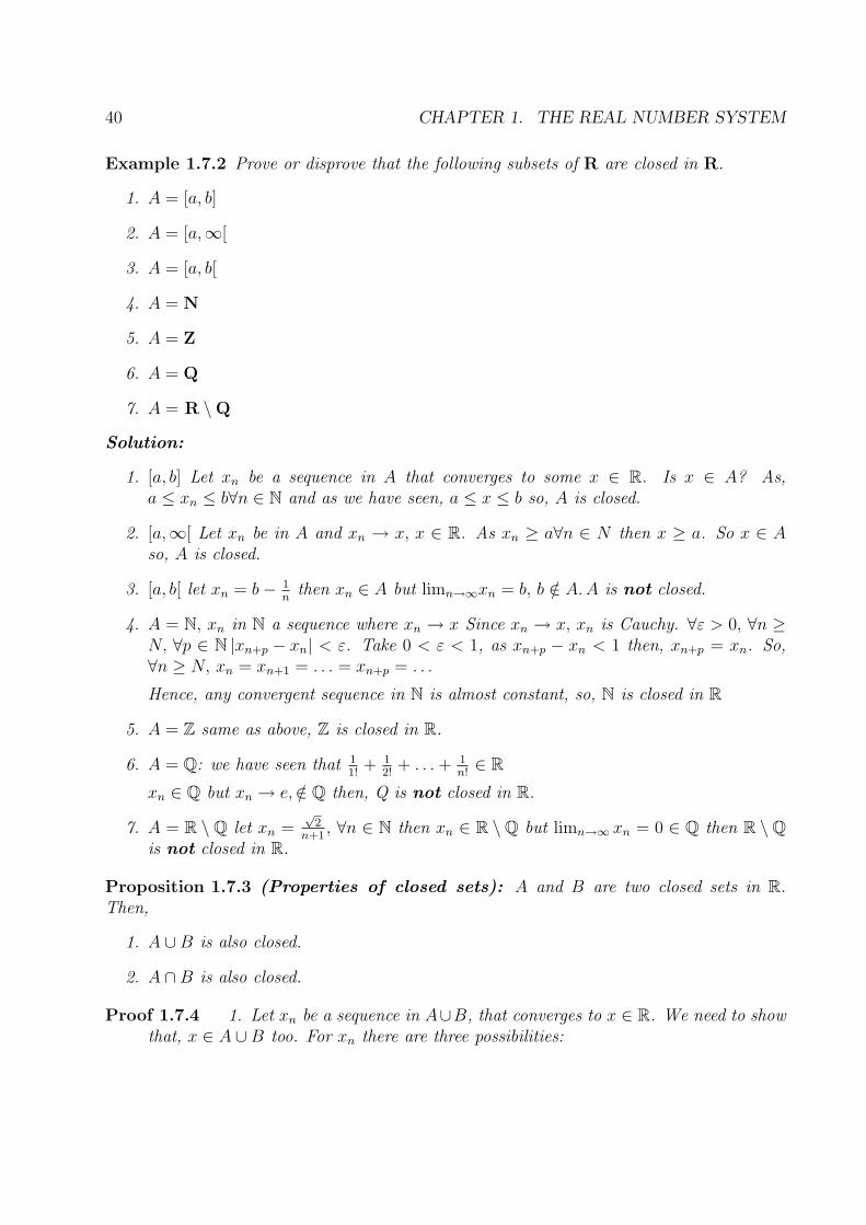
Example 1.7.2 Prove or disprove that the following subsets of R are closed in R.
1. A = [a, b]
2. A = [a,∞[
3. A = [a, b[
4. A = N
5. A = Z
6. A = Q
7. A = R \ Q
Solution:
1. [a, b] Let xn be a sequence in A that converges to some x ∈ R. Is x ∈ A? As,a ≤ xn ≤ b∀n ∈ N and as we have seen, a ≤ x ≤ b so, A is closed.
2. [a,∞[ Let xn be in A and xn → x, x ∈ R. As xn ≥ a∀n ∈ N then x ≥ a. So x ∈ Aso, A is closed.
3. [a, b[ let xn = b − 1n
then xn ∈ A but limn→∞xn = b, b /∈ A. A is not closed.
4. A = N, xn in N a sequence where xn → x Since xn → x, xn is Cauchy. ∀ε > 0, ∀n ≥N, ∀p ∈ N |xn+p − xn| < ε. Take 0 < ε < 1, as xn+p − xn < 1 then, xn+p = xn. So,∀n ≥ N, xn = xn+1 = . . . = xn+p = . . .
Hence, any convergent sequence in N is almost constant, so, N is closed in R
5. A = Z same as above, Z is closed in R.
6. A = Q: we have seen that 11!
+ 12!
+ . . . + 1n!
∈ R
xn ∈ Q but xn → e, /∈ Q then, Q is not closed in R.
7. A = R \ Q let xn =√
2n+1
, ∀n ∈ N then xn ∈ R \ Q but limn→∞ xn = 0 ∈ Q then R \ Qis not closed in R.
Proposition 1.7.3 (Properties of closed sets): A and B are two closed sets in R.Then,
1. A ∪ B is also closed.
2. A ∩ B is also closed.
Proof 1.7.4 1. Let xn be a sequence in A∪B, that converges to x ∈ R. We need to showthat, x ∈ A ∪ B too. For xn there are three possibilities:

1.7. ELEMENTARY TOPOLOGY OF R 41
(a) xn ∈ A for all but finitely many n. Then, x ∈ A
(b) xn ∈ B for all but finitely many n. Then, x ∈ B
(c) xn ∈ A for infinitely many n and xn ∈ B for infinitely many n Then x ∈ A ∩ B
So at any case, x ∈ A ∪ B, hence A ∪ B is closed.
2. Let xn in A ∩ B, that converges to some x ∈ R \ Q. As xn ∈ A, xn ∈ B for all n ∈ N.Since A and B are closed, x ∈ A and x ∈ B then x ∈ A ∩ B then A ∩ B is closed.
Remark:
1. ∪n≥1
[1
n.1 − 1
n
]= ]0, 1[
This shows that, the union of infinitely many closed sets need not be closed.
2. Any finite set F ⊆ R is closed.
F = {a1, a2, . . . , an}F = {a1} ∪ {a2} ∪ . . . ∪ {an}. As each {ai} is a closed set, F is closed.
3. The intersection of any family, (finite or not) of closed sets (Fα)α∈I is closed.
F = ∩α∈IFα
Theorem 1.7.5 Let A ⊆ R be a bounded set ( �= ∅) and α = sup A, β = inf A. Then, if Ais closed, α ∈ A and β ∈ A.
Proof 1.7.6 α = sup A ⇔{ ∀x ∈ A,α ≥ x
∀ε > 0,∃xε ∈ A : xε > α − ε
Now let ε = 1, 12, 1
3, . . . , 1
n. Denote xn ∈ A that correspond to ε = 1
nso that xn > α − 1
n.
In that way we get a sequence, (xn)n≥1 in A such that, α − 1n
< xn ≤ α. Then, xn → α asxn in A and A is closed α ∈ A.
Similarly, β ∈ A.
Remark: Converse is false.
Example 1.7.7 Let A = {−1} ∪ ]0, 1[ ∪ {2}sup A = 2, xn =
1
n∈ A, but limn→∞ xn = 0 /∈ A
inf A = −1
Finding Approximating sequences: Let A ⊆ R be a set and x ∈ R.Problem: When is there a sequence xn in A converges to x?
Theorem 1.7.8 Let A ⊆ R be any set and L ∈ R be any point. Then there exists a sequencexn in A : xn → L ⇔ ∀ε > 0, ]L − ε, L + ε[ ∩ A �= ∅

42 CHAPTER 1. THE REAL NUMBER SYSTEM
Proof 1.7.9 (=⇒) Suppose that there exists a sequence xn in A that converges to L. So wehave ∀ε > 0,∃N ∈ N, ∀n ≥ N, xn ∈ ]L − ε, L + ε[ ∩ A �= ∅
(⇐=) Suppose that, ∀ε > 0, ]L − ε, L + ε[ ∩ A �= ∅. So for ε = 1 this intersection is notempty. Take any point in it and call it x1.
For ε =1
2, this intersection is not empty. Take any point in it and call it x2.
...
For ε =1
n, this intersection is not empty. Take any point in it and call it xn. In this
way, construct a sequence xn such that xn ∈]L − 1
n, L +
1
n
[∩ A, ∀n ≥ 1. Hence, xn ∈ A
and |xn − L| <1
nso xn → L.
Example 1.7.10 We have seen that, ∀ε > 0, ∀x ∈ R, ]x − ε, x + ε[ ∩ Q �= ∅Hence, ∀x ∈ R, ∃xn ∈ Q : xn → x
Example 1.7.11 We have seen that, ∀ε > 0, ∀x ∈ R. ]x − ε, x + ε[ ∩ (R/Q) �= ∅.Hence, ∀x ∈ R, ∃ qn ∈ (R/Q) : qn → x
Exercise: Show that given x ∈ R there exists a sequence xn in the set A ={a + b
√2 : a, b ∈ Z
}.
That converges to x.
Definition 1.7.12 A subset A of R is said to be an open set if AC = R/A is closed in R.
Example 1.7.13 Q is not open since R/Q is not closed. So Q and R/Q are neither opennor closed.
Example 1.7.14 The set A = ]a, b[ is an open set, since R/A = ]∞, a] ∪ [b,∞[ is closed.(]∞, a] is closed and [b,∞[ is closed.) Hence A is open.
Theorem 1.7.15 Let A ⊆ R be any set then A is open ⇔ ∀x ∈ A, ∃ε > 0 such that]x − ε, x + ε[ ⊆ A.
Proof 1.7.16 (=⇒) Suppose A is open and x ∈ A. For a contradiction, suppose ∀ε > 0]x − ε, x + ε[ � A i.e. ∀ε > 0, ]x − ε, x + ε[ ∩ AC �= ∅.By the above theorem there exists a sequence xn in AC that converges to x as AC is closed.
x ∈ AC so x /∈ A.Hence, ∃ ε > 0 : ]x − ε, x + ε[ ⊆ A(⇐=) Suppose that ∀x ∈ A, ∃ε > 0 : ]x − ε, x + ε[ ⊆ A. Let us see that A is open, i.e.
AC is closed. Let (xn)n∈N be a sequence in AC that converges to some x ∈ R. If x /∈ AC
then x ∈ A. So for some ε > 0, ]x − ε, x + ε[ ⊆ A. As xn → x, xn ∈ ]x − ε, x + ε[ for allbut finitely many n. So, xn ∈ A for all but finitely many n.(contradiction). So, x ∈ AC andAC is closed. So, A is open.

1.8. CLOSURE AND INTERIOR OF A SET 43
Consequences:
1. A countable set can not be open.
2. A subset A ⊆ R is open iff A is a union of open intervals; A = ∪α∈I ]aα, bα[
3. A = [a, b[ is neither open nor closed.
4. If A is open and bounded, if α = sup A, and β = inf A then neither α ∈ A nor β ∈ A
Example 1.7.17 A = ]a, b[
1.8 Closure and Interior of a Set
Definition 1.8.1 Given any set A ⊆ R,
1. The closure of A is the smallest closed set that contains A.
2. The interior of A is the largest open set contained in A.
Question: Do these sets exist?Remark: Let (xn)n∈N be any bounded sequence. Let l = lim inf xn and L = lim sup xn.
Then, ∀ε > 0, ∃n ∈ N, ∀n ≥ N, L − ε ≤ xn ≤ L + ε
Let A ={x ∈ R : x = limn→∞an, for some sequence (an)n∈N in A
}.
Thus, x ∈ A ⇔ ∃ an ∈ A, an → x.
Theorem 1.8.2 For any set A
1. A is closed in R.
2. A ⊇ A.
3. A = A iff A is closed in R.
4. A is the smallest closed set that contains A.
Proof 1.8.3 1. First remark that if A = ∅, A = ∅, then A is closed. So, supposeA �= ∅. Let us see that the set O, where O = R/A is open. (As we know, O is open⇔ ∀x ∈ O, ∃ ε > 0, ]x − ε, x + ε[ ⊆ O ).
Let x ∈ O. We want to prove that there is ε > 0 such that ]x − ε, x + ε[ ⊆ O. If this wasnot the case we would have, ∀ε > 0 ]x − ε, x + ε[ ∩ A �= ∅. Then by “ApproximationTheorem”, there exists a sequence (xn)n∈N in A that converges to x.
So, ∀ε > 0, xn ∈ ]x − ε, x + ε[ for all but finitely many n. Fix one of these n’s.Say n = p, so that xp ∈ ]x − ε, x + ε[. Then choose ε′ > 0 small enough such that

44 CHAPTER 1. THE REAL NUMBER SYSTEM
]xp − ε′, xp + ε′[ ⊆ ]x − ε, x + ε[. Since xp ∈ A, there is a sequence yk in A thatconverges to xp. So, yk ∈ ]xp − ε′, xp + ε′[ for all but finitely many k ∈ N. This impliesthat, ]x − ε, x + ε[ ∩ A �= ∅ ∀ε > 0. Again by “Approximation Theorem”, there existsa sequence (an)n∈N in A that converges to x. So, x ∈ A (Contradiction). So for someε > 0, ]x − ε, x + ε[ ⊆ O. Hence O is open, A is closed.
2. Let x ∈ A. Let a constant sequence a0 = a1 = a2 = . . . = an = . . . = x. Then an → x.So, x ∈ A, hence A ⊇ A
3. If A = A, then A is closed, since A is closed. If A is closed, then A = A.
4. Let B be a closed set that contains A. So if an ∈ A, and (an)n∈N converges to some x,then x ∈ B. Hence A ⊆ B.
Definition 1.8.4 The set A is said to be the closure of A.
Example 1.8.5 Find Q and R/Q.Q = {x ∈ R : x = limn→∞rn for some rn ∈ Q} = RR/Q = {x ∈ R : x = limn→∞rn for some rn ∈ R/Q} = R.
∀A ⊆ R ∀x ∈ R, ∃ an ∈ A : an → x ⇔ ∀ε > 0 ]x − ε, x + ε[ ∩ A �= ∅
Example 1.8.6 Let A = ]a, b[. Then, A = [a, b]. (bn = b − 1n∈ A)
Example 1.8.7 Let A =
{1
n: n = 1, 2, ...
}. Then, A = A ∪ {0}.
Example 1.8.8 Let A =
{1
n+
1
m: n = 1, 2, . . . , m = 1, 2, . . .
}.
Then, A = A ∪{
1
m: m = 1, 2, . . .
}∪ {0}
Example 1.8.9 Let A =
⎧⎨⎩ 1
n+
1
m+
1
q:
n = 1, 2, . . .m = 1, 2, . . .q = 1, 2, . . .
⎫⎬⎭.
Then A = A ∪{
1
m+
1
n: m = 1, 2, . . . , n = 1, 2, . . .
}∪ {0}
Definition 1.8.10 (Interior of a Set A) Let A ⊆ R be any set. Define◦A as follows:
◦A is the union of all open intervals ]a, b[ contained in A. a = b =⇒ ]a, b[ = ∅. So, there
is always (empty or not) some open interval in A. Of course if A = ∅, then A◦ = ∅. This
set◦A is called the interior of A.
Theorem 1.8.11 1.◦A is open.

1.8. CLOSURE AND INTERIOR OF A SET 45
2. A ⊇ ◦A
3. A =◦A⇔ A is open.
4.◦A is the largest open set contained in A.
Proof 1.8.12 1. As the union of any open sets is open, it is open.
2. A ⊇ ◦A is obvious.
3. If A =◦A, then A is open, since
◦A is open. If A is open, then A is a union of open
intervals (=◦A)
4. Let B ⊆ A, B is open. Let x ∈ B. Then, as B is open ∃ε > 0 such that
]x − ε, x + ε[ ⊆ B. Then, ]x − ε, x + ε[ ⊆ A. So x ∈ ◦A. Hence B ⊆ ◦
A.
Example 1.8.13 Find◦Q,
◦N and
◦R/Q.
•◦Q= ∅, since Q does not contain any open interval.
•◦
R/Q= ∅, since R/Q does not contain any open interval.
• ◦N= ∅, since N does not contain any open interval.
• ◦Z= ∅, since Z does not contain any open interval.
•◦
[a, b]= ]a, b[
46 CHAPTER 1. THE REAL NUMBER SYSTEM
1.8.1 Exercises IV
1. Let X = {a0, a1, . . . , an, . . .}, where (an)n∈N is a convergent sequence in R with L =limn→∞an.
F be the set of the cluster points of (an)n∈N. Show that X = X ∪ F .
2. Let X = {tan n : n ∈ N}. Find X.
3. Let X = Q\N. Find X.
4. Let X = Q\Z. Find X.
5. Let X ={
1n
+ 1m
: n = 1, 2, 3, . . . , m = 1, 2, 3, . . .}. Find X.
6. Let (an)n∈N and (bn)n∈N be two convergent sequences in R with
L = limn→∞an and S = limn→∞bn. Put A = {an + bn : n ∈ N}, B = {an + bm : n ∈N, m ∈ N}. Find A and B.
7. For A = { nm
: n ∈ N, m = 1, 2, 3 . . .}, find A.
8. Let A and B be two nonempty subsets of R. Show that A + B ⊇ A + B and A × B ⊇A × B. Here A + B = {a + b : a ∈ A, b ∈ B} and A × B = {a × b : a ∈ A, b ∈ B}.
9. Show that for any countable subset◦A= ∅.
10. Let A be a closed subset of R. Show that◦A= ∅ iff R\A = R.
11. Let A be any nonempty proper subset of R and B = A\ ◦A. Show that B is closed and
◦B= ∅.
12. Let O be an open subset of R and A be an arbitrary subset of R. Show that
(a) If O ∩ A = ∅, then O ∩ A = ∅ too.
(b) We have O ∩ A ⊆ O ∩ A ⊆ O ∩ A.
13. Let A be a subset of R. Show that◦A= ∅ iff given any interval ]a, b[ there exists a
subinterval ]c, d[ of ]a, b[ such that ]c, d[ ∩ A = ∅.
14. Let A = {x ∈ R : x2 > 2} and B = {x ∈ R : x2 ≥ 2}. Show that A = B and◦B= A.
15. Let A be a nonempty bounded subset of R and δ(A) = δ(A). Is δ(A) = δ(◦A)?
16. Let O1 and O2 be two open sets with O1 = R and O2 = R. Show that O1 ∩ O2 = R.

Chapter 2
Minkowski and Holder Inequalities
For 1 ≤ p ≤ ∞ there is a unique q ∈ ]1,∞[ 1
p+
1
q= 1.
So, pq = p + q the number p is said to be the “conjugate of q”If p = 2 =⇒ q = 2.
If p =√
2 =⇒ q =
√2√
2 − 1.
If p = 1, then we take q = ∞.If q = 1, then we take p = ∞.
So, ∀ p ∈ ]1,∞[ , ∃ q ∈ ]1,∞[ 1
p+
1
q= 1
Now, let a, b ∈ R+. Then, (a − b)2 ≥ 0. So, a2 + b2 ≥ 2ab. Equivalently,
1
2a2 +
1
2b2 ≥ ab Eq 3.1
As1
2+
1
2= 1, we can expect that,
1
pap +
1
qbq ≥ ab,
(1 < p < ∞1
p+
1
q= 1
)
Lemma 2.0.14 For a, b ∈ R+ 1 < p < ∞ and1
p+
1
q= 1. The inequality,
ap
p+
bq
q≥ ab
holds.
Proof 2.0.15 If a = 0 or b = 0, there is nothing to prove. So, Suppose a > 0 and b > 0,then dividing the inequality (Eq 3.1) by bq, we obtain
apb−q
p+
1
q≥ ab1−q Eq 3.2
Put x = ab1−q (so, x > 0). Then xp = apbp−qp. Hence, Eq 3.2 becomes
xp
p+
1
q≥ x Eq 3.3
47

48 CHAPTER 2. MINKOWSKI AND HOLDER INEQUALITIES
Let f : [0,∞[ → R, f(x) =xp
p+
1
q− x. (Eq 3.2) is equivalent to
f(x) ≥ 0, ∀x ∈ [0,∞[ Eq 3.4
Now, f ′(x) = xp−1 − 1 = 0. So, x = 1. Hence, at x = 1, f has an extremum.As f ”(x) = (p − 1)xp−2 and f ”(x) = p − 1 > 0, we conclude that f has an absolute
minimum at x = 1.
As f(1) =1
p+
1
q− 1 = 0, we see that f(x) ≥ 0, ∀x ∈ [0,∞[. So, (Eq 3.4) holds, so (Eq
3.1) holds. For x = (x1, x2, x3, . . . , xn) ∈ Rn, we define the p-norm of xn as:
‖x‖ p = sup {|x1| , |x2| , |x3| , . . . , |xn|}. We want to prove that
{ ‖x + y‖p ≤ ‖x‖p + ‖y‖p and
‖x × y‖1 ≤ ‖x‖p × ‖y‖q
(1 < p < ∞ and1
p+
1
q= 1, (xy = x1y1 + · · · + xnyn))
For 1, ‖x + y‖1 ≤ ‖x‖1 + ‖y‖1 is obvious.For p = ∞, ‖x + y‖∞ ≤ ‖x‖∞ + ‖y‖∞.
Theorem 2.0.16 (Holder inequality) For 1 < p < ∞ and x, y ∈ Rn,‖x × y‖1 ≤ ‖x‖p × ‖y‖q.
Proof 2.0.17 If ‖x‖p = 0 or ‖y‖p = 0, then there is nothing to prove. So, suppose ‖x‖p > 0and ‖y‖p > 0.
Let ai =xi
‖x‖p
, bi =yi
‖y‖p
. Then by the preceding inequality,1
p
xpi
‖x‖pp
+1
q
ypi
‖y‖pp
≥ |xi|‖x‖p
|yi|‖y‖p
.
Adding them from p = 1 to p = n, we get:
1
p
n∑p=1
|xi|p
‖x‖pp
+1
q
n∑p=1
|xi|p
‖y‖p q≥
n∑p=1
|xi|p|yi|p
‖x‖p ||y||q
1 ≥
n∑i=1
|xi| |yi|
‖x‖p ‖y‖q
i.e. ||xy||1 ≤ ‖x‖p ||y||q. For p = q = 2, the Holder inequality becomes:
n∑i=1
|xi| |yi| ≤√
|x1|p + . . . + |xp|p√
|y1|p + . . . + |yp|p (Cauchy Schwartz Inequality)
Theorem 2.0.18 (Minkowski Inequality) ‖x + y‖p ≤ ‖x‖p + ‖y‖p.
Proof 2.0.19 For p = 1,‖x + y‖1 = |x1 + y1| + . . . + |xn + yn| ≤ |x1| + |y1| + . . . + |xn| + |yn| ≤ ||x||1 + ‖y‖1
For p = ∞, ‖x + y‖∞ = max{|x1 + y1| , . . . , |xn + yn|} ≤ max{|x1| + |y1| , . . . , |xn| + |yn|}≤ max{|x1| , . . . , |xn|} + max{|y1| , . . . , |yn|}

49
For 1 ≤ p ≤ ∞, ‖xi + yi‖p = |xi + yi|p−1 × |xi + yi| ≤ |xi + yi|p−1 |xi| + |xi + yi|p−1 |yi|,so that
n∑i=1
|xi + yi|p ≤n∑
i=1
|xi + yi|p−1 |xi| +n∑
i=1
|xi + yi|p−1 |yi|Now, by Holder inequality,
n∑i=1
|xi + yi|p−1 |xi| ≤(
n∑i=1
|xi + yi| (p−1)q
) 1q(
n∑i=1
|xi|p) 1
p
=
(n∑
i=1
|xi + yi|p) 1
q(
n∑i=1
|xi|p) 1
p
.
n∑i=1
|xi + yi|p−1 |yi| ≤(
n∑i=1
|xi + yi| (p−1)q
) 1q(
n∑i=1
|yi|p) 1
p
=
(n∑
i=1
|xi + yi|p) 1
q(
n∑i=1
|yi|p) 1
p
.
Hence,
(n∑
i=1
|xi + yi|p)1
≤(
n∑i=1
|xi + yi|p) 1
q
[‖xp‖ + ‖yp‖]
Hence,
(n∑
i=1
|xi + yi|p) 1
p
≤ [‖xp‖ + ‖yp‖] i.e. ‖xp + yp‖ ≤ ‖xp‖ + ‖yp‖.
Example 2.0.20b∫a
f(x)g(x)dx ≤(
b∫a|f(x)|p dx
) 1p
×(
b∫a|g(x)|p dx
) 1p
.

50 CHAPTER 2. MINKOWSKI AND HOLDER INEQUALITIES

Chapter 3
Metric Spaces (Basic Concepts)
1. Metric Spaces: Definition and Properties of the Real Numbers
2. Topology of Metric Spaces (Open Sets, Closed Sets, etc.)
3. Basic topological concepts. (Interior, Closure, boundary of a set etc.)
4. Accumulation Points and Isolated Points of a Set
5. Density and Separability
6. Relativization
7. Lindolf Theorem
3.1 Metrics and Metric Spaces
Let X be any set. ( �= ∅). A mapping d : X × X → [0,∞[ is said to be a “distance” or“metric” if
1. ∀x, y ∈ X, d (x, y) = 0 ⇐⇒ x = y
2. ∀x, y ∈ X, d (x, y) = d (y, x)
3. ∀x, y ∈ X, d (x, y) ≤ d (x, z) + d (z, y) “triangle inequality”
Then the pair (X, d) is said to be a metric space.
Example 3.1.1 1. X = N, Z, Q or R where metric is d (x, y) = |x − y|. Then (X, d) isa metric space. This metric d is said to be the ”usual metric” of R.
2. Let X = Rn and for 1 ≤ p ≤ ∞, dp (x, y) = ‖x − y‖p. Then by Minkowski Inequality,dp is a metric on Rn.
For p = 2, the metric d2 (x, y) =√|x1 − y1|2 + · · · + |xn − yn|2 is said to be the “Eu-
clidean metric” on Rn.
51

52 CHAPTER 3. METRIC SPACES (BASIC CONCEPTS)
3. Let X be any set and d be defined by d (x, y) =
{1 if x �= y0 if x = y
.Then d is a metric,
known as the “discrete metric”. Every set has at least the discrete metric. So everyset is a metric space.
4. Let X be any set and f : X → R be a one-to-one function. Put df (x, y) = |f (x) − f (y)|.Then df is a metric on X. e.g. X = R, f (x) = arctan x.
Then df (x, y) = |arctan (x) − arctan (y)| is a metric on R.
5. Let E be any set and X = B (E) = {f : E → R : f is bounded on E}.Let d∞ (f, g) = supx∈E |f (x) − g (x)| . d∞ is called the “supremum metric”.
Definition 3.1.2 Let (X, d) be a m.s., x ∈ X and ε > 0 given.
1. The set Bε (x) = {y ∈ X : d (x, y) < ε} is said to be an open ball centered at x withradius ε.
2. The set B′ε (x) = {y ∈ X : d (x, y) ≤ ε} is said to be a closed ball.
3. The set Sε (x) = {y ∈ X : d (x, y) = ε} is said to be a sphere.
Example 3.1.3 Let X = R2, d = d2.Bε (0) = {(x, y) ∈ R2 : x2 + y2 < ε2}B′
ε (0) = {(x, y) ∈ R2 : x2 + y2 ≤ ε2}Sε (0) = {(x, y) ∈ R2 : x2 + y2 = ε2}
Example 3.1.4 Let X = R2, d = d1.B1 (0) = {(x, y) ∈ R2 : |x| + |y| < 1}d = d∞ : B1 (0) = {(x, y) ∈ R2 : d∞ ((x, y) , (0, 0)) = max {|x| , |y|} < 1}.
3.2 Open Sets and Closed Sets
Definition 3.2.1 Let (X, d) be a metric space and A ⊆ X a set. We say that A is open⇐⇒ for any x ∈ A, ∃ε > 0 such that Bε (x) ⊆ A.
This is equivalent to say that a set A is open iff A is a union of a family of open balls.For X = R, d (x, y) = |x − y| Bε (x) = ]x − ε, x + ε[.
Example 3.2.2 On X put the discrete metric d. Then,
Bε (x) = {y ∈ X : d (x, y) < ε} =
{ ∅ if ε ≤ 1{x} if ε > 1
. Hence, any set A is open for this
metric. ∀x ∈ A, ∃ε > 0 (take ε < 1) Bε (x) = {x} ⊆ A.
Proposition 3.2.3 In any metric space (X, d) , every open ball Bε (x) is an open set.

3.2. OPEN SETS AND CLOSED SETS 53
Proof 3.2.4 Let y ∈ Bε (x). So d (x, y) < ε. Let 0 < ε′ < ε−d (x, y). Then Bε′ (y) ⊆ Bε (x).Indeed, for z ∈ Bε′ (y),d (x, z) ≤ d (x, y) + d (y, z) < d (x, y) + ε′ = d (x, y) + ε − d (x, y) = ε.Hence, z ∈ Bε (x), i.e. Bε′ (y) ⊆ Bε (x). So Bε (x) is an open set.
Definition 3.2.5 Let (X, d) be a metric space. Let τd be the collection of all open subsetsof X. This collection τd is said to be the “topology of X defined by d”.
Proposition 3.2.6 (Basic Properties of τd) Let (X, d) be any metric space. Then:
1. ∅ ∈ τd and X ∈ τd.
2. O1, O2 ∈ τd =⇒ O1 ∩ O2 ∈ τd.
3. (Oα)α∈I is a family in Υd =⇒ ∪α∈IOα ∈ τd.
Proof 3.2.7 1. ∅ is open by “intuition”.
2. Let O1, O2 be open sets. Let x ∈ O1 ∩ O2. Then x ∈ O1 and x ∈ O2.
Since O1 is open ∃ ε1 > 0 : Bε1 (x) ⊆ O1.
Since O2 is open ∃ε2 > 0 : Bε2 (x) ⊆ O2.
Let ε = min {ε1, ε2}. Then Bε (x) ⊆ O1 ∩ O2. So, O1 ∩ O2 is open.
3. Let (Oα)α∈I be any family of open sets. Let O = ∪α∈IOα. Let x ∈ O, then x ∈ Oα forsome α ∈ I. As Oα is open there is an ε > 0 such that Bε (x) ⊆ Oα ⊆ O. Hence, O isopen.
Remark: The intersection of infinitely many open sets need not to be open. Indeed, let
X = R, d (x, y) = |x − y| . Then, ∩n≥1
]− 1
n,1
n
[= {0} is closed.
Definition 3.2.8 Let (X, d) be a metric space. A set F ⊆ X is said to be closed if FC isopen.
Theorem 3.2.9 (Characterization of closed sets) Let (X, d) be a metric space andA ⊆ X a set. Then, A is closed ⇐⇒ ∀x ∈ X\A, ∃ ε > 0 : Bε (x) ∩ A = ∅.
Proof 3.2.10 (=⇒) Suppose that A is closed. Let x ∈ X\A be any point. Then sinceO = X\A is open ∃ε > 0 : Bε (x) ⊆ O, i.e. Bε (x) ∩ A = ∅.
(⇐=) Suppose that ∀x ∈ X\A, ∃ ε > 0 : Bε (x) ∩ A = ∅.This means that ∀x ∈ X\A, ∃ ε > 0 : Bε (x) ⊆ X\A. So X\A is open. Hence, A is
closed.

54 CHAPTER 3. METRIC SPACES (BASIC CONCEPTS)
Example 3.2.11 In any metric space (X, d), every finite set F = {a1, . . . , an} is closed. ByTheorem 3.2.9 it is enough to show the following:
∀x /∈ F, ∃ ε > 0 : Bε (x) ∩ F = ∅.Let x /∈ F . So d (x, ai) �= 0. Let ε =
1
2min {d (x, ai) : i = 1, . . . , n}. Then ε > 0. Now
Bε (x) ∩ F = ∅. Hence F is closed.
Example 3.2.12 Let X = R, d (x, y) = |x − y|.Then F = [a, b] , F = N, F = Z, F = [a,∞[ are closed.
Proposition 3.2.13 (Properties of Closed Sets) Let (X, d) be any m.s., F be the col-lection of the closed sets in X. Then;
1. ∅ ∈ F and X ∈ F .
2. F1, F2 ∈ F =⇒ F1 ∪ F2 ∈ F .
3. The intersection of any family of closed sets (Fα)α∈I is closed.
Proof 3.2.14 1. True by definition.
2. Let F1, F2 be two closed sets. Let x ∈ X\(F1 ∪ F2).
=⇒ ∃ε1 > 0 : Bε1(x) ∩ F1 = ∅ and ∃ε2 > 0 : Bε2(x) ∩ F2 = ∅. Let ε = min {ε1, ε2}.Then Bε(x) ∩ F1 ∪ F2 = ∅. Hence, F1 ∪ F2 is closed.

3.2. OPEN SETS AND CLOSED SETS 55
3.2.1 Exercises I
1. Let d be a metric on a set X. Show that
(a) ∀x, y, z ∈ X, |d(x, y) − d(y, z)| ≤ d(x, z).
(b) For xn, yn, x, y in X, |d(xn, yn) − d(x, y)| ≤ d(xn, x) + d(yn, y)
2. Let (X, d) be a metric space. For x, y ∈ X, define d′ by d′(x, y) = min{1, d(x, y)}.
(a) Show that d′ is also a metric on X.
(b) For 0 < ε < 1, Bε(x, d) = {y ∈ X : d(x, y) < ε} = Bε(x, d′) where Bε(x, d′) ={y ∈ X : d′(x, y) < ε}.
(c) Deduce that τd = τd′ .
3. Let (X, d) be a metric space. For x, y in X, define d′ by d′(x, y) =d(x, y)
1 + d(x, y). Show
that
(a) The function ϕ : [0,∞[ → [0,∞[ defined by ϕ(x) =x
1 + xis increasing.
(b) For any x, y ∈ [0,∞[ ,x + y
1 + x + y≤ x
1 + x+
y
1 + y.
(c) d′ is a metric on X.
(d) Fix x ∈ X. ∀ ε > 0, ∃ ε′ > 0 : Bε′(x, d′) ⊆ Bε(x, d).
(e) ∀ ε > 0, ∃ ε′ > 0 : Bε′(x, d) ⊆ Bε(x, d′).
(f) Deduce that τd = τd′ .
56 CHAPTER 3. METRIC SPACES (BASIC CONCEPTS)
3.3 Basic Topological Concepts
Definition 3.3.1 (Closure of a Set) Let (X, d) be a m.s. and let A ⊆ X be any set. LetA = {B ⊆ X : B ⊇ A, B is closed}. A �= ∅, since at least X ∈ A. Let A = ∩B∈AB. Then,A is said to be the closure of A.
Proposition 3.3.2 1. A is closed.
2. A is the smallest closed set containing A.
Proof 3.3.3 1. A is closed, since intersection of any family of closed sets is closed.
2. A ⊇ A since each B ∈ A contains A. So A is the smallest closed set containing A.
Theorem 3.3.4 (Characterization of the closure) Let (X, d) be any m.s., A any setand x ∈ X be any point. Then x ∈ A ⇐⇒ ∀ε > 0, Bε (x) ∩ A �= ∅.
Proof 3.3.5 Let x ∈ A. If we had some ε > 0 such that Bε (x)∩A = ∅, then we would haveA ⊆ X\Bε (x). Let B = X\Bε (x). Then B is closed and A ⊆ B. So A ⊆ B. This meansthat Bε (x)∩A = ∅. This is not possible since x ∈ Bε (x)∩A. This contradiction shows that∀ε > 0 Bε (x) ∩ A �= ∅.
Conversely, suppose ∀ε > 0, Bε (x) ∩ A �= ∅. Let us see that x ∈ A. Let B ⊇ A and Bclosed. We have to show that x ∈ B. If this was not the case, we would have x ∈ BC. AsBC is open, for some ε > 0, Bε (x) ⊆ BC. So B ∩ Bε (x) = ∅. In particular A ∩ Bε (x) = ∅,which is not possible. So x ∈ B, so x ∈ A.
Example 3.3.6 Let X = R, d (x, y) = |x − y|. Then Q = R and R\Q = R.
Example 3.3.7 Let X = Rn, d =Euclidean metric. Let us see that Qn = Rn.Let x ∈ Rn and ε > 0. We need to show that Bε (x)∩Qn �= ∅, i.e. ∃ r = (r1, . . . , rn) ∈ Qn
such that (x1 − r1)2 + · · · + (xn − rn)2 < ε2. Let ri ∈ Q be such that |xi − ri| <
ε√n. Then
(x1 − r1)2 + · · · + (xn − rn)2 < ε2.
Proposition 3.3.8 (Properties of the Closure Operation) Let (X, d) be a metric spaceand A,B be two subsets of X. Then,
1. A is closed ⇐⇒ A = A.
2. A = A.
3. A ⊆ B =⇒ A ⊆ B.
4. A ∪ B = A ∪ B.
5. A ∩ B ⊆ A ∩ B.

3.3. BASIC TOPOLOGICAL CONCEPTS 57
Proof 3.3.9 1. Always true from the definition.
2. Follows from 1.
3. If A ⊆ B, then A ⊆ B, too. Hence A ⊆ B.
4. As A ⊆ A ∪ B, B ⊆ A ∪ B. By 3=⇒A ⊆ A ∪ B, B ⊆ A ∪ B =⇒ A ∪ B ⊆ A ∪ B.
For the reverse inclusion; as A ⊆ A, B ⊆ B =⇒ A ∪ B ⊆ A ∪ B. Since the union oftwo closed sets is closed, A ∪ B is closed. Hence, by 3, A ∪ B ⊆ A ∪ B.
5. As A ∩ B ⊆ A, A ∩ B ⊆ B. By 3=⇒A ∩ B ⊆ A, A ∩ B ⊆ B =⇒ A ∩ B ⊆ A ∩ B.
Example 3.3.10 We do not have A ∩ B = A ∩ B.Let X = R, and d be usual metric. (|x − y|).Let A = Q, B = R\Q. Then A ∩B = ∅. So A ∩ B = ∅. On the other hand A = R, B =
R. So A ∩ B = R.
Definition 3.3.11 (Interior of a Set) Let (X, d) be any metric space and A ⊆ X beany set. Let A = {B ⊆ X : B is open, B ⊆ A } .A is nonempty since at least ∅ ∈ A. Let◦A= ∪B∈AB. This is clearly the largest open set contained in A. This set
◦A is said to be
“the interior of A”.
Theorem 3.3.12 (Characterization of the interior) Let (X, d) be a m.s. A ⊆ X, x ∈X. Then x ∈ ◦
A⇐⇒ ∃ε > 0 : Bε (x) ⊆ A.
Proof 3.3.13 (=⇒) Let x ∈ ◦A. As
◦A is open, by definition, ∃ε > 0 : Bε (x) ⊆ ◦
A. SoBε (x) ⊆ A.
(⇐=) Let ε > 0 be such that Bε (x) ⊆ A. Then this Bε (x) ∈ A. So Bε (x) ⊆ ◦A⊆ A.
Example 3.3.14 1. Let X = R, d (x, y) = |x − y|.◦Q= ∅,
◦R�Q= ∅, ◦
Z= ∅, ◦N= ∅,
◦[a, b]= ]a, b[.
2. Let X = Rn, d = d2. A = R × {0} =⇒ ◦A= ∅.
3. Let X = Rn, d = d2. A = Rn−1 × {0} =⇒ ◦A= ∅.
Proposition 3.3.15 (Properties of the interior operation)
1. A is open ⇐⇒ ◦A= A.
2.
◦◦A=
◦A.
58 CHAPTER 3. METRIC SPACES (BASIC CONCEPTS)
3. A ⊆ B =⇒ ◦A⊆ ◦
B
4.◦
(A ∪ B) ⊇ ◦A ∪ ◦
B
5.◦
(A ∩ B)=◦A ∩ ◦
B
Proof 3.3.16 1. Always true from the definition.
2. Follows from 1.
3. Let A ⊆ B. Then◦A⊆ B. Hence
◦A⊆ ◦
B since◦B is the largest open set contained in B.
4. A ⊆ A ∪ B, B ⊆ A ∪ B =⇒ ◦A⊆
◦(A ∪ B)
◦B⊆
◦(A ∪ B)=⇒ ◦
A ∪ ◦B⊆
◦(A ∪ B).
5. As A ∩ B ⊆ A, A ∩ B ⊆ B, =⇒◦
(A ∩ B)⊆ ◦A,
◦(A ∩ B)⊆ ◦
B=⇒◦
(A ∩ B)⊆ ◦A ∩ ◦
B.
Conversely,◦A ∩ ◦
B⊆ A∩B. As◦A ∩ ◦
B is open and contained in A∩B,◦A ∩ ◦
B⊆◦
(A ∩ B).
Example 3.3.17 Let X = R, d (x, y) = |x − y|.A = Q, B = R\Q =⇒ ◦
A= ∅, ◦B= ∅. But
◦(A ∪ B)= R.
Proposition 3.3.18 (Interior-closure connection) Let (X, d) be a m.s. A ⊆ X. Then,
1.(A)C
=◦(
AC)
.
2.( ◦A)C
= (AC).
Proof 3.3.19 1. Let x ∈ X be any point. Then, x ∈◦(
AC)⇐⇒ ∃ε > 0 : Bε (x) ⊆ AC ⇐⇒
∃ε > 0 : Bε (x) ∩ A = ∅ ⇐⇒ x /∈ A ⇐⇒ x ∈ (A)C .
2. Follows directly from 1.
Definition 3.3.20 Let (X, d) be a m.s. A ⊆ X. The set ∂A = A\ ◦A is said to be the
boundary of A.
Example 3.3.21 Let X = R2, d = d2. Let A = {(x, y) ∈ R2 : x2 + y2 < 1}. Then,
A = {(x, y) ∈ R2 : x2 + y2 ≤ 1} and A is open. So◦A = A =⇒ ∂A = {(x, y) ∈ R2 : x2 + y2 = 1}.
Example 3.3.22 Let X = R, d =usual metric, A = Q. Then A = R.◦A= ∅. So ∂A = R.

3.4. ACCUMULATION AND ISOLATED POINTS OF A SET 59
Example 3.3.23 Let X = R, d =usual metric, A = [a, b[. Then A = [a, b] ,◦A= ]a, b[. So
∂A = {a, b}.Proposition 3.3.24 (Properties of the Boundary)
1. For any set A ⊆ X, ∂A is always a closed set. Since ∂A = A\ ◦A= A∩
( ◦A)c
= A∩(Ac)
is closed.
2. ∂A = ∂(AC). Clear from 1.
3. A is closed iff ∂A ⊆ A.
4. A is open iff ∂A ∩ A = ∅.
3.4 Accumulation and Isolated Points of a Set
Definition 3.4.1 Let (X, d) be a m.s. and A ⊆ X be a set. We want to classify the pointsof A. For x ∈ A and ε > 0 arbitrary, Bε (x) ∩ A �= ∅. So, only one of the following mayhappen:
1. ∃ε > 0 : Bε (x) ∩ A = {x}. In this case we say that x is an isolated point of A.
2. ∀ε > 0 : Bε (x) ∩ A\ {x} �= ∅. In this case we say that x is an accumulation pointof A.
Remark: An isolated point of A is always in the set A but an accumulation point mayor may not be in A.
Example 3.4.2 Let X = R, d (x, y) = |x − y|1. A = N. Then A = N = N. For n ∈ N, if 0 < ε < 1, ]n − ε, n + ε[ ∩ N = {n}. So,
every point of N is an isolated point.
2. A = Q. Then Q = R. Let x ∈ R and ε > 0 be arbitrary.
Since ]x − ε, x + ε[ contains infinitely many rational numbers, certainly ]x − ε, x + ε[∩Q\ {x} �= ∅.Hence, every x ∈ R is an accumulation point of Q.
3. A =
{1
n: n = 1, 2, 3, . . .
}. Then A = A ∪ {0} . ∀ε > 0, ]−ε, ε[ ∩ A is an infinite set.
So, 0 is an accumulation point.
For x =1
n, for 0 < ε < min
{1
n− 1
n + 1,
1
n − 1− 1
n
},
]1
n− ε,
1
n+ ε
[∩ A =
{1
n
}.
So, that any x =1
nis an isolated point.
60 CHAPTER 3. METRIC SPACES (BASIC CONCEPTS)
Let, for any A ⊆ X, A′ ={x ∈ A : x is an accumulation point
}. Then clearly A = A ∪ A′.
Thus A is closed ⇐⇒ A′ ⊆ A.
Definition 3.4.3 • If A = A′, then we say that A is perfect.
• If every x ∈ A is an isolated point, then we say that A is discrete.
Example 3.4.4 A = [a, b] is a perfect set.
Example 3.4.5 A = N, A = Z is discrete. Any finite set is discrete.
Example 3.4.6 Let A =
{1
n+
1
m: n = 1, 2, . . . , m = 1, 2, . . .
}. Then
A = A ∪{
1
n: n = 1, 2, . . .
}∪ {0}.
A′ ={
1n
: n = 1, 2, . . .} ∪ {0}. A′′ = {0}. A′′′ = ∅.
Proposition 3.4.7 Let x ∈ A be a point. Then, x is an accumulation point ⇐⇒ ∀ε >0, Bε (x) ∩ A is infinite.
Proof 3.4.8 (⇐=) is trivial.
(=⇒) For a contradiction suppose, for some ε > 0, Bε (x)∩A is finite, say Bε (x)∩A ={x0, . . . , xn}. Let O = Bε (x) \F , where F = {x0, . . . , xn} − {x}. Then O is open andx ∈ O. So for some ε′ > 0, Bε′ (x) ⊆ O. Hence, Bε′ (x) ⊆ Bε (x) and Bε′ (x) ∩ F = ∅or Bε′ (x) ∩ F = {x}. Hence, Bε′ (x) ∩ A\ {x} = ∅. This contradicts the definition ofaccumulation point. So, ∀ε > 0, Bε (x) ∩ A is infinite.

3.4. ACCUMULATION AND ISOLATED POINTS OF A SET 61
3.4.1 Exercises II
All the sets below are the subsets of R and on R the metric is its usual metric.
1. Show that, for any set A, A′ is a closed set.
2. If A �= ∅ and bounded and infinite, show that then A′ �= ∅.
3. If A is uncountable, then show that A′ �= ∅.
4. If A is open, then show that A has no isolated point.
5. If A is dense R, then show that A has no isolated point.
6. For A =
{1
n+
1
m+
1
p: n = 1, 2, 3, . . . , m = 1, 2, 3, . . . , p = 1, 2, 3, . . .
}, find A,A′, A′′, A′′′
and A′′′′.
7. Show that for any set A, ∂A ⊆ ∂A and ∂A◦ ⊆ ∂A.
8. Let a ∈ A. Show that;
(a) a is an accumulation point of A iff A has a sequence (xn)n∈N with xn �= a for alln such that xn → a.
(b) a is an isolated point of A iff every sequence (xn)n∈N in A that converges to a iseventually constant.
9. If a ∈ ∂A, then show that there exist two sequences (xn)n∈N and (yn)n∈N convergingto a such that xn ∈ A for all n ∈ N and yn /∈ A for all n ∈ N.
10. Show that a subset A of R can have at most countably many isolated points. Deducethat every discrete subset of R is countable.

62 CHAPTER 3. METRIC SPACES (BASIC CONCEPTS)
3.5 Density and Separability
Definition 3.5.1 Let (X, d) be a m.s. If M ⊆ X and M = X, then we say that M is densein X.
Example 3.5.2 Q is dense in R. R\Q is dense in R. Qn is dense in Rn.
Theorem 3.5.3 Let (X, d) be a m.s and M ⊆ X be a set. Then, The followings are equiv-alent:
1. M = X
2. ∀O ⊆ X, where O is open: O ∩ M �= ∅.3. ∀x ∈ X, ∀ε > 0 : Bε (x) ∩ M �= ∅.
Definition 3.5.4 A metric space (X, d) is said to be separable, if there is a countable setM ⊆ X such that M = X.
Example 3.5.5 1. Let X = R, d (x, y) = |x − y|. Then as Q = R and Q is countable, Ris separable.
2. Let X be any set. On X put the discrete metric d (x, y) =
{1 if x �= y0 if x = y
. Then
in this metric space (X, d) every set A is at the same time closed and open. So,∀A ⊆ X, A = A. Hence, the only dense set is X itself.
Conclusion: (X, d) is separable ⇐⇒ X is countable.
3. (Rn, d2) is separable since Qn = Rn
Theorem 3.5.6 Let (X, d) be a m.s. Suppose that we have in this m.s. an uncountablefamily (Oα)α∈I of nonempty, pairwise disjoint, open sets. (i.e., ∀α �= β, Oα∩Oβ = ∅). Thensuch a metric space cannot be separable.
Proof 3.5.7 Let M ⊆ X be any set such that M = X. By Theorem 3.5.3, M ∩Oα �= ∅. Letxα ∈ M∩Oα be any point. As Oα∩Oβ = ∅, for α �= β, xα �= xβ. Let N = {xα : α ∈ I}. ThenN is uncountable and N ⊆ M . This means that any dense subset M of X is uncountable.So (X, d) cannot be separable.
Example 3.5.8 Let E be an infinite set. X = B (E) = {ϕ : E → R : ϕ is bounded}. Ford (ϕ, ψ) = sup |ϕ (x) − ψ (x)| , X becomes a m.s.
Let us see that the m.s. (X, d) is not separable. As, E is infinite, 2E is uncountable.∀A ∈ 2E, let ϕA = χA. Then ϕA ∈ X. For A �= B, d (ϕA, ϕB) = supx∈E |χA (x) − χB (x)| =
1. Let B 12(ϕA) be the open ball in X with radius
1
2and center at ϕA. Put OA = B 1
2(ϕA).
Then OA ∩ OB = ∅ for A �= B. Hence, (OA)A∈2E is an uncountable family of nonempty,pairwise disjoint, open sets in X. So (X, d) is not separable.
If E = N, then B (E) = {ϕ : N → R : ϕ is bounded} = the space of bounded sequences.The set B (N) is denoted by l∞.

3.5. DENSITY AND SEPARABILITY 63
3.5.1 Exercises III
All the sets below are subsets of R and the metric on R is its usual metric.
1. Find an uncountable closed set K such that◦K= ∅.
2. If K �= ∅, F �= ∅, both are closed and one of them is bounded, show that then, K + Fis closed.
3. Show that the sets F1 = Z and F2 =√
2Z are closed but F1 + F2 is dense in R.
Hint: First, show that every subgroup G of (R, +) is either dense or discrete.
4. Let A be any set ( �= ∅) and B any open set ( �= ∅). Show that the set A + B is open.
5. Let A �= ∅ be any set. Show that A = ∩k≥1
(A +
]− 1k, 1
k
[).
6. From 4 and 5 deduce that every closed subset A of R is the intersection of countablymany open sets and that every open set O is the union of countably many closed sets.
7. Let A = ∪n≥1
[n + 1
n, n + 1 − 1
n
], N∗ = N\{0}. Show that both A and N∗ are closed,
A ∩ N∗ = ∅ but d(A, N∗) = infa∈Ap∈N∗ |a − p| = 0.
8. Let I �= ∅ be an interval, A any set (∅ �= A �= R). Show that if I ∩ A �= ∅ andI ∩ AC �= ∅, then I ∩ ∂A �= ∅.
9. Let I = [a, b] and O0, O1, . . . , On, . . . be open sets such that I ⊆ ∪n∈NOn. Show that
there exists N ∈ N such that I ⊆ N∪n=0On.

64 CHAPTER 3. METRIC SPACES (BASIC CONCEPTS)
3.6 Relativization
Let X = R2, d = d2. Consider R as a subset of R2. (We identify R with x-axis, i.e.R ≡ R × {0}) Observe that for (x, 0) , (y, 0) in R × {0} . d2 ((x, 0) , (y, 0)) = |x − y|.
So that, the metric induced by d2 on R is just d (x, y) = |x − y|. Hence, we have twometric spaces (R, d) , (R2, d2) with R ⊆ R2, d2|R = d.
Now, observe also that for (x, 0) in R× {0} , Bε ((x, 0))∩R = ]x − ε, x + ε[× {0}. Now,let A ⊆ R be a set. We can consider A as a subset of R or as a subset of R2.
In the abstract case, we have a m.s. (X, d) a subset M ⊆ X, so that (M,d) is also a m.s.
Let A ⊆ M . Let AM
be the closure of A in M , and A be the closure of A in X.
Question: How are these sets related?
• For x ∈ X and ε > 0, Bε (x) = {y ∈ X : d (x, y) < ε}.• For x ∈ M and ε > 0, Bε (x) = {y ∈ M : d (x, y) < ε}
Then, it is clear that Bε (x) = Bε (x) ∩ M for x ∈ M .
Proposition 3.6.1 For A ⊆ M, AM
= A ∩ M .
Proof 3.6.2 Let x ∈ M . Then, x ∈ AM ⇐⇒ ∀ε > 0, Bε (x)∩A �= ∅ ⇐⇒ Bε (x)∩M ∩A =
Bε (x) ∩ A �= ∅ ⇐⇒ x ∈ A ∩ M . Hence, if A ⊆ M : A is closed in M means that AM
= A.A is closed in X means that A = A. For x ∈ M, Bε (x) is open in M , but it is not open
in X, unless M is open in X.
Proposition 3.6.3 Let (X, d) be a m.s. M ⊆ X and A ⊆ M . Then,
1. A is closed in (M, d) ⇐⇒ there exists a closed set F ⊆ X such that A = F ∩ M .
2. A is open in (M, d) ⇐⇒ there exists an open set O ⊆ X such that A = O ∩ M .
Proof 3.6.4 1. We have seen that AM
= A ∩M . So if A is closed in M , then AM
= A,so that A = A ∩ M , so we take F = A.
Conversely, if A = F ∩ M for some closed set F ⊆ X, then let us see that A isclosed in M . So, let x ∈ M\A. Then x /∈ F . As F is closed in X, there is anε > 0 : Bε (x) ∩ F = ∅. Then Bε (x) = Bε (x) ∩ M is a neighborhood of x in M and
Bε (x) ∩ A = ∅. Hence x /∈ AM
and AM
= A, so A is closed in M .
2. Apply 1 to B = M\A.
Example 3.6.5 Let X = R, d (x, y) = |x − y|. Let M = [0, 1[. Then the set A =
[0,
1
2
[is
open in M , but not in X. Indeed,
[0,
1
2
[=
]−1,
1
2
[∩ M, where
]−1,
1
2
[is open. The set
A =
[1
2, 1
[is closed in M . Indeed A =
[1
2, 1
[=
[1
2, 2
]∩ M , where
[1
2, 2
]is closed.

3.6. RELATIVIZATION 65
3.6.1 Exercises IV
1. Let (X, d1), (Y, d2) be 2 m.s. and Z = X × Y .
For z1 = (x1, y1) and z2 = (x2, y2) in Z, put d(z1, z2) = d1(x1, x2) + d2(y1, y2) andd′(z1, z2) = max{d1(x1, x2), d2(y1, y2)}
(a) Show that d and d′ are metrics on Z and d′ ≤ d.
(b) Let zn = (xn, yn) be a sequence in Z. Show that zn → z = (x, y) in (Z, d) iffxn → x in (X, d1) and yn → y in (Y, d2).
(c) Let A1 ⊆ X,A2 ⊆ Y . Show that in the m.s. (Z, d) we have A1 × A2 = A1 × A2.
(d) Let A1 ⊆ X,A2 ⊆ Y . Show that
i. A1 ×A2 is closed in the m.s. (Z, d) iff A1 is closed in (X, d1) and A2 is closedin (Y, d2).
ii. A1 × A2 is open in (Z, d) iff A1 is open in (X, d1) and A2 is open in (Y, d2).
(e) Show that (Z, d) is separable iff both spaces (X, d1) and (Y, d2) are separable.Deduce that (Rn, d1) is separable.
(f) Show that the m.s. (Z, d) is complete iff the spaces (X, d1) and (Y, d2) are com-plete.
2. Let (X, d1), (Y, d2) and Z = X × Y be as in the question 1 above. Let A ⊆ Z be anyset.
Show that A is closed in (Z, d) iff A is closed in (Z, d′). Deduce that τd = τd′ .
66 CHAPTER 3. METRIC SPACES (BASIC CONCEPTS)
3.7 Lindolf Theorem
Let (X, d) be a metric space.
Lemma 3.7.1 If (X, d) is separable, then there exists countably many open sets (Bn)n∈N
such that every open set O ⊆ X is a union of some of Bn’s.
Proof 3.7.2 Let M = {an : n ∈ N} be a dense subset in X. Consider the collection{Br (an) : n ∈ N, r > 0, r ∈ Q}. This is a countable set of open sets. Let us see that these
sets satisfy the conclusion of the lemma. Let O ⊆ X be any open set. As M = X, O∩M �= ∅.Let F = {an ∈ M : an ∈ O} i.e., F = O∩M . Since an ∈ O and O is open, there is a rationalnumber rn > 0 : Brn (an) ⊆ O. Let us see that ∪an∈F Brn (an) = 0.
Let x ∈ O. Since O is open, for some ε > 0, Bε (x) ⊆ O. Since M = X, B ε3(x)∩M �= ∅.
Hence, for some an ∈ F, an ∈ B ε3(x). Let rn > 0 rational such that
ε
3< rn <
ε
2. Then
x ∈ Brn (an). So, x ∈ ∪an∈F Brn (an). Hence O = ∪an∈F Brn (an).
Example 3.7.3 X = R, d (x, y) = |x − y|. The collection {]a, b[ : a, b ∈ Q} is countable.Moreover any open set O of R is a union of some of these intervals.
Corollary 3.7.4 If (X, d) is separable, then ∀M ⊆ X the space (M,d) is separable.
Proof 3.7.5 Let (Bn)n∈N be a sequence of open sets as in Lemma 3.7.1.Let F = {n ∈ N : Bn ∩ M �= ∅}. Let xn ∈ Bn ∩ M be any point for each n ∈ F . Let us
see that A = {xn : n ∈ F} is dense in M . Let O = O ∩ M be any nonempty open set of M .As O is a union of Bn’s, then O contains at least one point from A. So A is dense in M .
Theorem 3.7.6 (Lindolf) Let (X, d) be a separable m.s. and (Oα)α∈I any family of opensets. Then I has a countable subset I such that ∪α∈IOα = ∪α∈IOα.
Proof 3.7.7 Let (Bn)n∈N be a sequence of open sets as in Lemma 3.7.1. So any Oα is aunion of some of these Bn’s. Now, ∀n ∈ N let In = {α ∈ I : Oα ⊇ Bn}. Some of the In’s areempty but not all. Let F = {n ∈ N : In �= ∅}. For each n ∈ F , let α ∈ I be any point (HenceOαn ⊇ Bn). Let I = {αn : n ∈ F}. Let us see that ∪α∈IOα = ∪αn∈IOαn. The inclusion ⊇ istrivial. To prove the other inclusion, let x ∈ ∪α∈IOα. Then x ∈ Oα for some α ∈ I. ThisOα is a union of some Bn’s. So our x is in one of these Bn’s. Then x ∈ Bn ⊆ Oα. Then,as Bn ⊆ Oαn , x ∈ Oan. So, ∪α∈IOα = ∪αn∈IOαn.

Chapter 4
Convergence in a Metric Space
1. Limit and Cluster Points of a Sequence
2. Cauchy Sequences and Completeness
3. lim sup and lim inf Again
4.1 Limit and Cluster Points of a Sequence
Let (X, d) be a metric space and (xn)n∈N be a sequence in X. Then we say that;xn converges to a ∈ X if we have: ∀ε > 0, ∃N ∈ N : ∀n ≥ N, d (xn, a) < ε.
In this case we write limn→∞xn = a. Then xn → a ⇐⇒ ∀ε > 0, xn ∈ Bε (a) for all butfinitely many n.
Lemma 4.1.1 Limit is unique. If xn → a and xn = b, then a = b.
Proof 4.1.2 Suppose a �= b. Let ε = d(a,b)3
. Then Bε (a) ∩ Bε (b) = ∅. As, xn → a, xn ∈Bε (a) for all but finitely many n ∈ N. So Bε (b) can contain at most xn for finitely many n.So xn � b. Hence a = b.
Example 4.1.3 Let X = Rm, let d = dp, 1 < p < ∞. Then any sequence xn in X is of theform xn = (an,1, an,2, . . . an,m). What does ”xn → a in Rm” mean?
For a = (a1, . . . , am), dp(xn, a) = (|an,1 − a1|p + . . . + |an,m − am|p)1p . Then,
xn → a ⇔ dp(xn, a) → 0 ⇔ an,i → ai, ∀ i = 1, 2, . . . , m. Thus xn → a in Rm iff “xn
converges to a coordinate-wise.”For p = 1, d1(xn → a) = (an,1 − an) + . . . + |an,m − am| → 0 ⇔ an,i → ai in R.For p = ∞, d∞(xn, a) = max{|an,i − ai| : 1 ≤ i ≤ m} → 0 ⇔ an,i → ai in R.
Example 4.1.4 Let E be any set. X = B(E) = {f : E → R : f is bounded}. On X we putthe metric d(f, g) = supx∈E|f(x) − g(x)|. Let (fn)n∈N be a sequence in X.
What does “fn → f” mean?
67

68 CHAPTER 4. CONVERGENCE IN A METRIC SPACE
fn → f ⇔ supx∈E
|fn(x)−f(x)| → 0 ⇔ ∀ ε > 0, ∃ N ∈ N,∀ n ≥ N, ∀x ∈ E, |fn(x)−f(x)| < ε
Uniform Convergence
Theorem 4.1.5 Let (X, d) be a m.s. A ⊆ X be a set and x ∈ X be a point. Then x ∈ A iffthere is a sequence an in A : an → x. So A = {x ∈ X : x is the limit of some sequence in A}
Proof 4.1.6 We have seen that x ∈ A ⇔ ∀ ε > 0, Bε(x) ∩ A �= ∅.(⇒) Suppose x ∈ A. Hence ∀ ε > 0, Bε(x) ∩ A �= ∅.Let ε = 1. Then take any point in B1(x) ∩ A, call it a1.
Let ε =1
2. Then take any point in B 1
2(x) ∩ A, call it a2.
Let ε =1
3. Then take any point in B 1
3(x) ∩ A, call it a3
...
Let ε =1
n. Then take any point in B 1
n(x) ∩ A, call it an.
In this way we construct a sequence an in A such that an ∈ B 1n(x)∩A, i.e. d(an, x) ≤ 1
n.
So, d(an, x) → 0, i.e. an → x.(⇐) Conversely suppose that for some sequence an in A, we have that an converges to
x. Then ∀ ε > 0, an ∈ Bε(x) for all but finitely many n ∈ N. Hence, Bε(x) ∩ A �= ∅. Sincean ∈ A, ∀ n ≥ 0.
Corollary 4.1.7 Let (X, d) be m.s. A ⊆ X. Then,A is closed ⇔ ∀ convergent sequence an in A, limn→∞an ∈ A.
Proof 4.1.8 A is closed ⇔ A = A. Then apply the Theorem 4.1.5.
Example 4.1.9 Let X = R2 with the Euclidean metric. d = d2. Let F be the graph of the
parabola y =1
xfor x > 0. Is F closed in R2? F = {(x,
1
x) : x > 0}
Let bn = (an,1
an
) that converges in R2 to some (x, y) ∈ R2. Then, by the result of the
preceding theorem, an → x and1
an
→ y. As1
an
→ y, x cannot be zero. So, y =1
x. Hence
(x, y) = (x,1
x) ∈ F . So F is closed.
4.2 Cluster Points of a Sequence
Definition 4.2.1 Let (X, d) be a m.s., (xn)n∈N a sequence in X. We say that a point a ∈ Xis a cluster point of the sequence iff for any ε > 0, xn ∈ Bε(x) for infinitely many n ∈ N.
Thus a is a cluster point of xn if ∀ε > 0, ∀ k ∈ N∃n > k : xnk∈ Bε(x).

4.3. THE SET OF THE CLUSTER POINTS OF A SEQUENCE XN 69
Proposition 4.2.2 If xn → x. Then x is the only cluster point of (xn)n∈N.
Remark: The converse of this proposition is false. Indeed, let xn = 1,1
2, 3,
1
4, 5, . . ..
Then 0 is the only cluster point but xn � 0.
Proposition 4.2.3 Let xn be a sequence in a m.s. (X, d) and a ∈ X. Then a is the onlycluster point of xn iff xn has a subsequence that converges to a.
Proof 4.2.4 Suppose a is a cluster point of xn. So ∀ ε > 0, xn ∈ Bε(a) for infinitely manyn.
Let ε =1
20. Let n0 be any integer such that xn0 ∈ B 1
20(a).
Let ε =1
2. Let n1 > n0 be any integer such that xn1 ∈ B 1
21(a).
...
Let ε =1
2k. Let nk > nk−1 be any integer such that xnk
∈ B 1
2k(a).
In this way we construct a subsequence xnkof xn such that d(xnk
, a) <1
2k→ 0 i.e.
xnk→ a as k → ∞.Conversely, suppose that xn has a subsequence xnk
that converges to a. Then ∀ ε >0, xnk
∈ Bε(a) for all but finitely many k or equivalently ∀ ε > 0, xn ∈ Bε(a) for infinitelymany n. Hence a is a cluster point.
4.3 The set of the cluster points of a sequence xn
Let xn be a sequence in a m.s. (X, d). PutF0 = {x0, x1, . . .}F1 = {x1, x2, . . .}...Fn = {xn, xn+1, . . .}...
and let F = ∩n∈N(Fn).
Example 4.3.1 In R. xn = (−1)n, then Fn = {−1, 1}. So Fn = {−1, 1}.Hence F = ∩n∈N(Fn) = {−1, 1}Let xn = 1,
1
2, 3,
1
4, 5, . . . Then Fn = Fn ∪ {0}. Hence F = ∩n∈N(Fn) = {0}.
Let xn = n. Then Fn = {n, n + 1, . . .}. So Fn = Fn, F = ∩n∈N(Fn) = ∅.Let xn be an enumeration of the rational numbers in [0, 1], then F = ∩n∈N(Fn) = [0.1]
Theorem 4.3.2 Let xn be a sequence in any m.s. (X, d) and F = ∩n∈N(Fn) as above. Thena ∈ X is a cluster point of xn, iff a ∈ F .

70 CHAPTER 4. CONVERGENCE IN A METRIC SPACE
Proof 4.3.3 Let a ∈ F be a point. So, a ∈ Fn ∀n ∈ N. Hence ∀ ε > 0, ∀ n ∈ N :Bε(a) ∩ Fn �= ∅, i.e. ∀ ε > 0, xn ∈ Bε(a) for infinitely many n.
Suppose a is a cluster point of xn. Then ∀ ε > 0, xn ∈ Bε(a) for infinitely many n. HenceBε(a) ∩ Fn �= ∅ ∀n ∈ N. So a ∈ Fn ∀ n ∈ N. Hence a ∈ F .
Question: When we have F �= ∅?
Example 4.3.4 Let X = B(E) (E any infinite set), B(E) =space of bounded functions.d(x, y) = supx∈E|x(x), y(x)|
Let ϕ0, ϕ1, . . . , ϕn, . . . be distinct points of E and ϕn = χ{ϕn}, where χA = { 1 x ∈ A0 x /∈ A
.
Consider the sequence {ϕn}n∈N in X. (Observe that |ϕn(x)| ≤ 1, ∀ x ∈ E).
Does this sequence have a cluster point in X?
Now, observe that, for n �= m, d(ϕn, ϕm) = supx∈E|χ{ϕn} − χ{ϕm}| = 1. This impliesϕn has no cluster points. Hence, for this sequence F = ∅. On the other hand, in (R, d)Bolzano-Weierstrass says that for any bounded sequence xn, the set F �= ∅. Hence, in (R, d)if xn is a bounded sequence, then F is a nonempty, closed, bounded set.
Hence α = inf F and β = sup F exist and α, β ∈ F.
Thus α = lim inf xn, β = lim sup xn
4.4 Bolzano-Weierstrass in Rm
A sequence xn in Rm, xn = (an,1, an,2, . . . , an,m), is bounded iff
‖x‖n =√
(an,1)1 + . . . + (an,m)2 ≤ M ∀ n ∈ N (for some M > 0).
So iff each (an,i)n∈N is bounded. (i = 1, 2, ..., m).
A subsequence of xn is of the form: xn,k = (ank,1, ank,2, . . . , ank,m)
Theorem 4.4.1 Every bounded sequence xn in Rm has at least one cluster point.
Proof 4.4.2 (an,1) is bounded in R so by Bolzano-Weierstrass in R. (an,1) has a convergentsubsequence (an1
k,1) that converges to some a1 ∈ R. Then, (an1k,2) is also bounded in R.
By Bolzano-Weierstrass in R. (an1k,2) has a convergent subsequence (an2
k,2) that convergesto some a2 ∈ R. Then (anm−1
k ,m) is bounded. By Bolzano-Weierstrass, it has a convergent
subsequence (anmk ,m) that converges to am ∈ R.
Let xnk= (anm
k ,1, anmk ,2, . . . , anm
k ,m). Then (xnk) is a subsequence of (xn) and
xnk→ (a1, . . . , am).

4.5. CAUCHY SEQUENCES AND COMPLETENESS 71
4.5 Cauchy Sequences and Completeness
4.5.1 Complete Metric Spaces
Let (X, d) be a m.s. Let (xn)n∈N be sequence in X. If xn → a, then we have: ∀ ε > 0, ∃ N ∈N, ∀ n ≥ N d(xn, a) <
ε
2. So,
∀ ε > 0, ∃ N ∈ N ∀ n ≥ N ∀ m ≥ N d(xn, xm) < ε. Eq 5.1
Hence any convergent sequence satisfies equation Eq 5.1
Definition 4.5.1 Any sequence xn satisfying the condition
∀ ε > 0 ∃ N ∈ N ∀ n ≥ N ∀ m ≥ N d(xn, xm) < ε Eq 5.2
is said to be “Cauchy.” Then every convergent sequence is Cauchy. The converse is false.
Example 4.5.2 Let X = R, d(x, y) = |Arc tan x − Arc tan y|. Now, let xn = n2. Thend(xn, xm) = |Arc tan n2 − Arc tan m2|. So that limn→∞, m→∞d(xn, xm) → 0.
So, ∀ ε > 0, ∃ N ∈ N, ∀ n ≥ N, ∀ m ≥ N, d(xn, xm) < ε. Hence xn is Cauchy in thism.s. (R, d).
But, there is no a ∈ R such that d(xn, a) = |Arc tan n2 − Arc tan a| → 0.
Example 4.5.3 Let X = R(N) = {ϕ : N → R : ϕ(n) �= 0 for all but finitely many n},d(x, y) = supn∈N|ϕ(n) − ψ(n)|.
Let ϕn = (1,1
2,1
3, . . . ,
1
n, 0, . . . , 0, . . .). Then,
ϕn+p − ϕn = (0, 0, . . . , 0,1
n + 1, . . . ,
1
n + p, 0, . . . , 0, . . .) so that,
d(ϕn, ϕn+p) = supk∈N|ϕn(k) − ϕn+p(k)| =1
n + 1→ 0 as n → ∞∀ p ∈ N.
So, ϕn is Cauchy. But there is no ϕ = (a1, a2, . . . , an, 0, . . . , 0, . . .) ∈ X for whichd(ϕn, ϕ) → 0.
Example 4.5.4 X = Q, (x, y) = |x − y|, xn = 1 +1
1!+ · · · + 1
n!.
Then xn is Cauchy in Q, but does not converge in Q.
Definition 4.5.5 A m.s. (X, d) is said to be complete if every Cauchy sequence xn in Xconverges to some x ∈ X.
Example 4.5.6 (R, d) d(x, y) = |x − y| is complete.
1. ∀ m ≥ 1, (R, d) d = d2 =Euclidean metric is a complete m.s. Indeed, xn = (xn,1, xn,2, . . . , xn,m).xn is Cauchy iff each component sequence (xn,i) is Cauchy in (R, d). So, converges toxi ∈ R, then xn → (x1, x2, . . . , xm)

72 CHAPTER 4. CONVERGENCE IN A METRIC SPACE
2. Let E be any set and X = B(E) = {Y : E → R: any bounded function}. For φ, ψ ∈ X,let d(φ, ψ) = supx∈E|φ(x), ψ(x)|
Theorem 4.5.7 (B(E), d) is complete.
Proof 4.5.8 Let φn be a Cauchy sequence in B(E). So we have:
∀ ε > 0, ∃ N ∈ N ∀n ≥ N, ∀m ≥ N, d(φn(x) − φm(x)) < ε (Eq 5.3)
In particular, for each x ∈ E, the sequence φn(x) is Cauchy R. So, since R is complete,(φn(x))n∈N converges to some αx ∈ R. Let φ : E → R be defined by φ(x) = αx.
Let us see that:
1. φ is bounded, i.e. φ ∈ B(E)
2. d(φn, φ) → 0.
In Eq 5.3, let m = N so that supx∈E|φn(x) − φN(x)| ≤ ε.
Then supx∈E|φn(x)| ≤ ε + supx∈E|φN(x)|, ∀n ≥ N .
i.e., ∀ x ∈ E, |φn(x)| ≤ ε + sup |φN(x)|, ∀ n ≥ N .
Letting n → ∞, we get that: ∀x ∈ E |φ(x)| ≤ ε + sup |φN(x)|. Hence φ is bounded. Soφ ∈ B(E).
Now, let us see that d(φn, φ) → 0. In Eq 5.3, let x ∈ E be any element so that:
∀ ε > 0, ∃ N ∈ N, ∀ n ≥ N, ∀ m ≥ N, d(φn(x)− φm(x)) < ε (Observe that N does notdepend on X )
Now, let m → ∞, we get that: ∀ε > 0, ∃ N ∈ N,∀ n ≥ N, ∀ x ∈ E |φn(x) − φ(x)| < ε
=⇒ ∀ε > 0, ∃ N ∈ N, ∀ n ≥ N, ∀ x ∈ E, sup |φn(x) − φ(x)| < ε.
Hence, d(φn, φ) → 0. So, (B(E), d) is complete.
4.5.2 Cluster Points of a Cauchy Sequence
Theorem 4.5.9 Let (X, d) be a m.s. and (xn)n∈N be a Cauchy sequence in X. Then eitherxn has no cluster points, or it has only one cluster point. In this later case, it converges tothis cluster point.
Proof 4.5.10 Suppose xn has a cluster point a ∈ X. Let us see that xn → a. Let us writewhat we have:
1. ∀ ε > 0, ∃ N ∈ N,∀n ≥ N, ∀m ≥ N, d(xn, xm) <ε
2
2. ∀ ε > 0, xn ∈ B ε2(a) for infinitely many n ∈ N

4.5. CAUCHY SEQUENCES AND COMPLETENESS 73
Let m ≥ N be such that xm ∈ Bε
2
(a). Then;
∀ n ≥ N d(xn, a) ≤ d(xn, xm)︸ ︷︷ ︸ + d(xm, a)︸ ︷︷ ︸ < ε
<ε
2(1)
<ε
2(2)
Hence xn → a.

74 CHAPTER 4. CONVERGENCE IN A METRIC SPACE

Chapter 5
Compactness
1. Definition and Characterization of Compact Sets
2. Sequential and Countable Compactness
3. Totally Bounded Sets:
5.1 Definition and Characterization of Compact Sets
5.1.1 Introduction
E = [0, 2π] and X = B(E) = {f : E → R : f is bounded}.On X we put the metric d(Φ, Ψ) = supx∈E|Φ(x) − Ψ(x)|. Let Φn(x) = cos(nx). Then
∀ n ∈ N ∀ x ∈ [o, 2π] | cos nx| ≤ 1.Question: Does Φn have a subsequence Φnk
that converges in (B(E), d)?No.
Now, let e1, e2, . . . , en, . . . be arbitrary points in [0, 2π] but Ψn = χen . Then Φn ∈B(E) d(Ψn, Ψm) = 1, ∀ n �= m. Hence no sequence of Ψn is Cauchy. Hence Ψn has noconvergent subsequence. Observe that ∀ n ∈ N, ∀ x ∈ E |Ψn(x)| ≤ 1. Hence the analog ofthe Bolzano-Weierstrass Theorem is not true in (B(E), d).
Question: Characterize the subsets K of B(E), for which Bolzano-Weierstrass holds.(i.e.every sequence Φn in K has a convergent subsequence.)
Definition 5.1.1 Let (X, d) be a m.s. K ⊆ X and (Oα)α∈I be a family of open sets. IfK ⊆ ∪α∈IOα then we say that (Oα)α∈I is any open covering of K.
(i.e. K ⊆ (Oα)α∈I ⇒ K ⊆ Oα1 ∪ Oα2 ∪ . . . ∪ Oαn .)
Definition 5.1.2 A subset K of X is said to be compact if whenever (Oα)α∈I is an opencovering of K, then there exists finitely many α1, α2, . . . , αn ∈ I such that K ⊆ Oα1∪. . .∪Oαn.(i.e. K ⊆ ∪α∈IOα =⇒ K ⊆ Oα1 ∪ Oα2 ∪ . . . ∪ Oαn)
75
76 CHAPTER 5. COMPACTNESS
Example 5.1.3 Let X = R, d(x, y) = |x − y|. Let K = N, On =
]n − 1
2, n +
1
2
[. Then
N ⊆ ∪n∈NOn but whatever n1, . . . , nk N � On1 ∪ . . . ∪ Onk. So N is not compact.
Example 5.1.4 Let K = ]0, 1] and On =
]1
n, 1 +
1
n
[. Then K ⊆ ∪n≥1On but whatever
n1, . . . , nk, K � On1 ∪ . . . ∪ Onk. so K is not compact.
K is compact⇔⎧⎨⎩
1) K is closedand
2) Any sequence (xn) in K has a convergent subsequence
5.1.2 Properties of Compact Sets:
Proposition 5.1.5 Let (X, d) be a m.s. Any compact set is closed in X.
Proof 5.1.6 Let K be compact. Take a point x ∈ X\K. We want to show that for some
ε > 0, Bε(x) ∩ K = ∅. Since x /∈ K, for every y ∈ K, d(x, y) > 0. Let εy =d(x, y)
2.
Then K ⊆ ∪y∈KBεy(y). As K is compact and Bεy(y) is open, there exist y1, . . . , yn such that
K ⊆ Bεy1(y1) ∪ . . . ∪ Bεyn
(yn). Let 0 < ε <1
2min{εy1 , . . . , εyn}. Then Bε(x) ∩ K = ∅, since
Bε(x) ∩ [Bεy1(y1) ∪ . . . ∪ Bεyn
(yn)]
= ∅. Hence K is closed in X.
Theorem 5.1.7 1. The union of two compact sets K1, K2 of X is compact.
2. The intersection of a compact set K with a closed set F is compact.
Proof 5.1.8 1. Let K = K1∪K2. Let for some open family (Oα)α∈I , K ⊆ ∪α∈IOα. ThenK1 ⊆ ∪α∈IOα and K2 ⊆ ∪α∈IOα. As K1 and K2 are compact, K1 = Oα1 ∪ . . . ∪ Oαn
and K2 = Oβ1 ∪ . . . ∪ Oβm for some α1, . . . , αn and β1, . . . , βm in I. Then K ⊆Oα1 ∪ . . . ∪ Oαn ∪ Oβ1 ∪ . . . ∪ Oβm. Hence K is compact.
2. Let (Oα)α∈I be an open family such that K ∩F ⊆ ∪α∈IOα. Then K ⊆ (∪α∈IOα)∪FC.As K is compact and FC is open K ⊆ Oα1 ∪ . . . ∪ Oαn ∪ FC for some α1, . . . , αn ∈ I.Hence K ∩ F ⊆ Oα1 ∪ . . . ∪ Oαn. So K ∩ F is compact.
Example 5.1.9 Let (X, d) any m.s. Then,
1. A one-point set K = {a} is compact.
2. If K = {a1, . . . , an} then K is compact.
3. If (X, d) is discrete, then any compact set K ⊆ X is finite.
Indeed, in any discrete metric space every set A is open and closed. In particular,∀ x ∈ X, the set {x} is open. If K is compact, from K ⊆ ∪x∈K{x} we get thatK ⊆ {x1} ∪ . . . ∪ {xn} for some x1, . . . , xn ∈ K. Hence K is finite.

5.1. DEFINITION AND CHARACTERIZATION OF COMPACT SETS 77
4. For any metric space, if xn ∈ X and xn → x, then the set K = {xn : n ∈ N} ∪ {x} isa compact set.
Indeed, suppose that K ⊆ ∪α∈IOα, Oα’s are open in X. Then x ∈ Oα′ for some α′ ∈ I.Hence ∃ N ∈ N : xn ∈ Oα′ ∀ n ≥ N . Then we say x0 ∈ Oα0 , x1 ∈ Oα1 , . . . , xN ∈ OαN
.Hence, K ⊆ Oα1∪Oα2∪. . .∪OαN
∪Oα′. So K is compact. X is compact ⇐⇒ WheneverX = ∪α∈IOα, we have X = Oα1 ∪ . . . ∪ Oαn for some α1, . . . , αn ∈ I.
5. Now, let (X, d) be a m.s. and K ⊆ X a set. Then K is compact ⇐⇒ (K, d) is acompact m.s.
K ⊆ ∪α∈IOα ⇒ K = α ∈ I∪(Oα ∩ K) = ∪α∈IOα, Oα = Oα ∩ K is open in (K, d).
Hence (K, d) is compact⇔whenever K = ∪α∈IOα, Oα is open in (K, d),
K = Oα1 ∪ . . . ∪ Oαn for some α1, . . . αn ∈ I. (or K ⊆ Oα1 ∪ . . . ∪ Oαn).
6. If K ⊆ M ⊆ X. Then to say that K is compact in (M, d) is equivalent to saying thatK is compact in X.
Since in either cases, this is equivalent to say that (K, d) is compact. So compactnessis absolute notion.
Example 5.1.10 R ⊆ R2 ⊆ . . . ⊆ Rn ⊆ . . .. K ⊆ R be a set. On Rn we put d2. Then,K is compact in R ⇔ K is compact in R2
⇔ K is compact in R3
...⇔ K is compact in Rn
...
Proposition 5.1.11 Any compact m.s. (K, d) is separable.
Proof 5.1.12 Let ε > 0 be given. Then K ⊆ ∪x∈KBε(x). As K is compact, there exists a
finite set Fε = {x1, . . . , xi} such that K ⊆ Bε(x1) ∪ . . . ∪ Bε(xi). Let ε = 1, then ε =1
2,
then ε =1
3, . . . So that for ε =
1
nwe have a finite set Fn ⊆ K such that K ⊆ ∪x∈FnB 1
n(x).
Let A = ∪n≥1Fn. Then A is countable and A ⊆ K. Let us see that A = K.Indeed if we had y ∈ K\A, there would be an ε > 0 such that Bε(y) ∩ A = ∅ i.e.
Bε(y) ∩ Fn = ∅ ∀ n ≥ 1. Let n be large enough to have1
n<
ε
2. As y ∈ K ⊆ ∪x∈FnB 1
n(x),
d(x, y) <1
nfor some x ∈ Fn. But then d(x, y) > ε, so Bε(y)∩Fn �= ∅, which is not possible.
So A = K and K is separable.
Proposition 5.1.13 Let (X, d) be any m.s. K ⊆ X compact, Fn ⊆ X closed such thatK ⊇ F0 ⊇ F1 ⊇ . . . ⊇ Fn ⊇ . . . and each Fn �= ∅ then ∩n∈NFn �= ∅ (Nested IntervalTheorem)

78 CHAPTER 5. COMPACTNESS
Proof 5.1.14 For a contradiction, suppose that ∩n∈NFn = ∅. Then ∪n∈NFCn = X. So as
K ⊆ X, K ⊆ ∪n∈NFCn . As K is compact, K ⊆ FC
0 ∪ . . . ∪ FCn for some n ∈ N. But
FC0 ∪ . . . ∪ FC
n = FCn , since F0 ⊇ . . . ⊇ Fn. so K ⊆ FC
n . Hence Fn ⊆ KC. as Fn ⊆ K,Fn ⊆ K ∩ KC = ∅, so Fn = ∅, which is not possible.
Hence ∩n∈NFn �= ∅.
Example 5.1.15 Let X = R, d(x, y) = |x − y|. Fn = [n, +∞[, then F0 ⊇ . . . ⊇ Fn ⊇ . . .each Fn is closed, Fn �= ∅ but ∩n∈NFn = ∅.
Our next aim is to prove the following theorem:
Theorem 5.1.16 Let (X, d) be m.s. and K ⊆ X a set.
Then K is compact ⇐⇒⎧⎨⎩
1) K is closedand2)Every sequence xn in K has a convergent subsequence xnk
Lemma 5.1.17 Let (X, d) be a m.s. and K ⊆ X a compact set. Then every sequence (xn)in K has a convergent subsequence (xnk
). (Equivalently every sequence xn has at least onecluster point x ∈ K).
Proof 5.1.18 Let xn be a sequence in K. Put Fn = {xn, xn+1, . . .} and F = ∩n∈N(Fn).We have to show that F �= ∅. As K is closed and Fn ⊆ K, Fn ⊆ K. So that we haveK ⊇ F0 ⊇ . . . ⊇ Fn ⊇ . . . and Fn �= ∅ ∀n ∈ N. Hence by the Nested Interval TheoremF = ∩n∈N(Fn) �= ∅. So xn has a cluster point.
Corollary 5.1.19 Any compact m.s. (X, d) is complete.
Proof 5.1.20 Let (xn)n∈N be a Cauchy sequence in X. As (X, d) is compact, (xn)n∈N hasa cluster point x ∈ X. But then, since any Cauchy sequence in any m.s. that has a clusterpoint converges to this point, we conclude that xn → x. So (X, d) is complete.
Example 5.1.21 Consider the m.s. (Q, d), d(x, y) = |x−y|. Let K = {x ∈ Q : 0 ≤ x ≤ 1}.Then K is not compact, since (K, d) is not complete.
Example 5.1.22 Let xn =1
3
[n∑
k=0
1!
k!
]is Cauchy, xn ∈ K but (xn)n∈N has no cluster point
in K.

5.2. SECOND CHARACTERIZATION OF COMPACT SETS 79
5.2 Second Characterization of Compact Sets
Definition 5.2.1 A m.s. (X, d) (or a subset of it) is said to be sequentially compact ifevery sequence (xn)n∈N in X has a cluster point x ∈ X.
Example 5.2.2 In (R, d) every closed and bounded set K is sequentially compact.
Lemma 5.2.3 Every sequentially compact m.s. (X, d) is separable.
Proof 5.2.4 For each ε > 0, let Aε be a maximal subset of X such that for any x �= y in
Aε, d(x, y) ≥ ε.( *)
Claim: Aε is finite. If it was not, we could choose infinite distinct points x0, x1, . . . , xn, . . .
(xi �= xj ∀ i �= j). Then, since (X, d) is sequentially compact, (xn)n∈N would have aconvergent subsequence yk = xnk
. Then (yk)k∈N would be Cauchy. But this is not possiblesince for k �= k′ d(yk, yk′) ≥ ε. So Aε is finite.
Next, for ε =1
n, denote the corresponding Aε as An(so ∀ x, y ∈ An, x �= y, d(x, y) ≥ 1
n).
Let A = ∪n≥1An. Then A is countable, since each An is finite. Let us see that A = X. If not,then there is an a ∈ X such that a /∈ A. Hence for some ε > 0, Bε(a) ∩ An = ∅. Let n be
such that1
n< ε. Since Bε(a)∩A = ∅, Bε(a)∩An = ∅, too. Hence ∀ x ∈ An, d(a, x) ≥ ε >
1
n.
But then An = An ∪ {a} satisfies (*). However this is not possible since An is a maximal
set satisfying (*). Hence A = X and X is separable.
Theorem 5.2.5 (Main Theorem): Let (X, d) be a m.s. and K ⊆ X a subset of it. ThenK is compact iff K is closed and every sequence (xn)n∈N in K has a cluster point.
Proof 5.2.6 We have already proved the implication (⇒).
(⇐) Suppose that K is closed and every sequence in K has a cluster point. Then by theLemma 5.2.3, the m.s. (K, d) is separable. Now, to prove that K is compact, let (Oα)α∈I
be a family of open sets in X such that K ⊆ ∪α∈IOα. Then K = ∪α∈I(Oα ∩ K) and eachOα = Oα ∩ K is open in (K, d). Now, as (K, d) is separable, by “Lindolf Theorem” I has acountable subset J such that K = ∪α∈J(Oα∩K). Relabelling Oα’s we can assume that J = N,so that K = ∪n∈N(On ∩K). Hence K ⊆ ∪n∈NOn. Then replacing On by On = O1 ∪ . . .∪On,we can assume that O0 ⊆ O1 ⊆ . . . ⊆ On ⊆ . . .
Let us see that K is contained in some On. If not then, for every n ∈ N, K � On, sothere is xn ∈ K\On. In that way we get a sequence (xn)n∈N in K. By hypothesis, (xn)n∈N
has a cluster point x ∈ K. As K ⊆ ∪n∈NOn, x ∈ ON for some N ∈ N. As ON is open andx ∈ ON , xn ∈ ON for infinitely many n ∈ N. Then ∃n > N such that xn ∈ ON but this isnot possible since xn /∈ On, so xn /∈ Op ∀ p ≤ n, a contradiction.
Hence, K ⊆ On for some n ∈ N, i.e. K is compact.

80 CHAPTER 5. COMPACTNESS
Example 5.2.7 1. Compact subsets of R: A subset K of R is compact iff K is closedand bounded.
Proof: Let K be compact. We have seen that every compact set in any m.s. is closed,so K is closed. Let us see that K is bounded. If it was not ∀n ∈ N ∃ xn ∈ K : |xn| > n.Such a sequence CANNOT HAVE a convergent subsequence. Hence K is bounded.
Conversely, suppose that K is closed and bounded. Then by Theorem 5.2.5 and BolzanoWeierstrass Theorem, K is compact.
2. Compact subsets of (Rn, d) where d is Euclidean metric: A subset K of Rn iscompact iff K is closed and bounded (i.e. supn∈N ||x||2 < ∞). (Same proof as above.)
3. Compact subsets of a discrete m.s. (X, d): A subset K of a discrete m.s. (X, d)is compact iff K is finite.
e.g. if K ⊆ Z or K ⊆ N, then K is compact iff K is finite.
4. Let E be an infinite set and X = B(E) the space of bounded functions with the metricd(ϕ, ψ) = supx∈E|ϕ(x) − ψ(x)|.
5. Let K = B′1(0) = {ϕ ∈ X : supx∈E|ϕ(x) ≤ 1|}.
Remark: In any m.s. (X, d) a set K ⊆ X is said to be bounded iff
δ(K) = supx,y∈Kd(x, y) < ∞ ⇔ ∃R > 0 : K ⊆ BR(x) for some x ∈ X ⇔ For somex0 ∈ K, supx∈K d(x0, x) < ∞. It is clear that K = B′
1(0) is closed and bounded in (X, d).But K is NOT COMPACT!
Let x1, . . . , xn, . . . ∈ E (xi �= xj, for i �= j). Let ϕn = χ{xn}. Then;
d(ϕn, ϕm) = supx∈E|ϕn(x) − ϕm(x)| = 1, ∀n �= m (* ).
On the other hand, ϕn ∈ K, ∀ n ∈ N, since |ϕn(x)| ≤ 1, ∀ x ∈ E, (*) shows that nosubsequence of ϕn is Cauchy, so no convergent subsequence of (ϕn)n∈N is convergent. HenceK is not compact.
5.3 Totally Bounded Sets
Definition 5.3.1 Let (X, d) be a m.s. A subset K ⊆ X is said to be totally bounded ifgiven any ε > 0, there exist finitely many points x1, . . . , xn ∈ K such that K ⊆ Bε(x1) ∪. . . ∪ Bε(xn).
Theorem 5.3.2 Let (X, d) be a complete m.s. and K ⊆ X a set. Then;
K is compact ⇐⇒ K is closed and is totally bounded.
To prove this theorem, we need to prove the following lemma:

5.3. TOTALLY BOUNDED SETS 81
Lemma 5.3.3 (Contour’s Nested Interval Theorem) Let (X, d) be a complete m.s.and F0 ⊇ F1 ⊇ . . . ⊇ Fn ⊇ . . . be nonempty closed sets, such that δ(Fn) → 0 as n → ∞.Then the intersection ∩n∈NFn is nonempty and contains just one point. (Here δ(Fn) =sup{d(x, y) : x, y ∈ Fn} is the ′′ diameter of F n”)
Proof 5.3.4 Let for each n ∈ N, xn ∈ F be an arbitrary point. Observe that, as F0 ⊇ F1 ⊇. . . ⊇ Fn ⊇ . . ., {xn, xn+1, . . .} ⊆ Fn. Let ε > 0 be arbitrary. As δ(Fn) → 0 there is N ∈ Nsuch that ∀n ≥ N δ(Fn) < ε. Hence ∀n ≥ N ∀ p ∈ N d(xn, xn+p) ≤ δ(Fn) < ε. This showsthat (xn)n∈N is a Cauchy sequence. As (X, d) is complete. (xn)n∈N converges to a pointa ∈ X. As {xn, xn+1, . . . , xn+p, . . .} ⊆ Fn and Fn is closed, a ∈ Fn ∀ n ∈ N. So a ∈ ∩n∈NFn.As δ(Fn) → 0, the intersection ∩n∈NFn cannot contain any point x �= a.
Remark: Let X = R, d(x, y) = |x − y|. Let Fn = {n, n + 1, . . . , n + p, . . .}. Then Fn isclosed and F0 ⊇ F1 ⊇ . . . ⊇ Fn ⊇ . . . So, ∩n∈NFn = ∅. (Hence δ(Fn) � 0).
Proof 5.3.5 proof of theorem 5.3.2
1. Suppose that K is compact. Then as we have seen that K is closed. Let ε > 0 be anynumber. Then, obviously K ⊆ ∪x∈KBε(x). As K is compact and each Bε(x) is open,K ⊆ Bε(x1) ∪ . . . Bε(xk) for some x1, . . . , xk ∈ K. So K is totally bounded.
2. Conversely, suppose that K is closed and totally bounded. i.e.
∀ ε > 0, ∃ x1, . . . , xk ∈ K : K ⊆ Bε(x1) ∪ . . . ∪ Bε(xk). Let us see that every sequence(xn)n∈N in K has a cluster point.
In (Eq 5.2) let ε = 1. Then ∃ a1, . . . , ap ∈ K : K ⊆ Bε(a1) ∪ . . . ∪ Bε(ap). So, forsome infinite F1 ⊆ N, (xn)n∈F1 is contained in one of these balls, say B1(a).
Let K1 = B′1(a1) ∩ K. Then K1 is totally bounded.
So with ε =1
2, K ⊆ B 1
2(b1) ∪ . . . B 1
2(bq) for some b1, . . . , bq ∈ K1.
As (xn)n∈F1 ⊆ K1 ⊆ B 12(b1) ∪ . . . ∪ B 1
2(bq), there is an infinite set F2 ⊆ F1 such that
(xn)n∈F2 is contained in one of these balls, say B 12(b1).
Let K2 = K1 ∩ B′12
(b1). Then K2 is totally bounded.
With ε =1
3, ∃ c1, . . . , ck ∈ K2, K2 ⊆ B 1
3(c1) ∪ . . . ∪ B 1
3(ck)
...
And so on. In this way, we construct K ⊇ K1 ⊇ . . . ⊇ Kn ⊇ . . . and δ(Kn) ≤ 2
n→ 0.
Hence ∩n∈NKn = {a} for some a ∈ K. Now, let
n1 ∈ F1 be such that xn1 ∈ K1
n2 ∈ F2, n2 > n1 be such that xn2 ∈ K2...
nk ∈ Fk, nk > nk−1 be such that xnk∈ Kk

82 CHAPTER 5. COMPACTNESS
Then by the proof of Lemma 5.3.3, yk = xnk→ a. Thus, a is a cluster point of (xn)n∈N .
So K is compact.
Example 5.3.6 Let l1 = {x = (xn)n∈N ∈ RN :∞∑
n=0
|x| < ∞}. For x ∈ l1,
||x||1 =∞∑
n=0
|xn| and d(x, y) = ||x− y||1. Then (l1, d) is a m.s. This m.s. is complete. Let
K ⊆ l1 be a set. Then,
K is compact⇐⇒
⎧⎪⎪⎪⎨⎪⎪⎪⎩
1◦) K is closed2◦) K is bounded:supx∈K ||x||1 < ∞3◦) limk→∞sup x = (xn)n∈N ∈ K
∞∑k=n
|xk| = 0

5.4. EXERCISES 83
5.4 Exercises
1. Let (X, d) be a metric space and A be a nonempty subset of X. For x ∈ X putd(x,A) = infa∈Ad(x, a). Show that
(a) d(x, A) = 0 iff x ∈ A.
(b) ∀ ε > 0 the set Fε = {x ∈ X : d(x,A) ≤ ε} is closed and A ⊆ Fε.
(c) ∀ ε > 0 the set Oε = {x ∈ X : d(x, A) ≤ ε} is open and A ⊆ Fε.
2. Let (X, d) be a metric space and A,B be 2 subsets of X (A �= ∅, B �= ∅). Putd(A,B) = inf(x,y)∈A×Bd(x, y). Show that
(a) if A is closed, B is compact and A ∩ B = ∅, then d(A,B) > 0.
(b) Assume A, B are compact and disjoint. Let ε =d(A,B)
3. Show that the sets
Oε = {x ∈ X : d(x,A) < ε} and Oε = {x ∈ X : d(x,B) < ε} are open,A ⊆ Oε, B ⊆ Oε and Oε ∩ Oε = ∅.
3. Let (X, d) be a m.s. and (xn)n∈N be a convergent sequence in X with a = limn→∞xn.Show that the set K = {xn : n ∈ N} ∪ {a} is compact.
4. Let (X, d) be a m.s. and K0 ⊇ K1 ⊇ . . . ⊇ Kn ⊇ . . . be nonempty compact sets. Showthat the set K = ∩n∈NKn is nonempty.
5. Let X = R, d(x, y) = |x − y| and Fn = {n, n + 1, n + 2, . . .}. Show that
F0 ⊇ F1 ⊇ . . . ⊇ Fn ⊇ . . . , Fn is closed and Fn �= ∅ for each n ∈ N but ∩n∈NFn = ∅.
6. Let l′ be the space of all the mappings ϕ : N → R such that∞∑
n=0
|ϕ(x)| < ∞. For
ϕ, ψ ∈ l′ put d(ϕ, ψ) =∞∑
n=0
|ϕ(n) − ψ(n)|. Show that
(a) d is a metric on l′.
(b) The set K = {ϕ ∈ l′ :∞∑
n=0
|ϕ(n)| ≤ 1} is closed and bounded.
(c) Let, for each n ∈ N, fn = χ{n}. Then, fn ∈ K and for n �= m, d(fn, fm) = 2.
(d) (fn)n∈N has no subsequence which is Cauchy.
(e) Show that although K is closed and bounded, it is not compact.
7. On R2 consider the Euclidean metric d2. Let F ⊆ R2 be closed and O ⊆ R2 be anopen set. Let K ⊆ R be a compact set. Show that

84 CHAPTER 5. COMPACTNESS
(a) The set A = ∪x∈K{y ∈ R : (x, y) ∈ F} is a closed set.
(b) The set B = ∩x∈K{y ∈ R : (x, y) ∈ O} is an open set.
8. Let K1, K2 be 2 nonempty compact subsets of R, d(x, y) = |x − y|. Show that the setK1 + K2 is also compact.
9. Let K be a compact subset of Rn, (d = d2) and ε > 0. Show that the set
Kε = {x ∈ Rn : d(x,K) ≤ ε} is also compact.
10. Let (X1, d1), (X2, d2) be two m.s., Y = X1 × X2 and
d((x1, x2), (x1, x2)) = max{d1(x1, x1), d2(x2, x2)}.11. Let K1 ⊆ X1 and K2 ⊆ X2 be compact sets. Show that the set K = K1 × K2 is
compact in (Y, d)

Chapter 6
Continuity
1. Definition and First Properties
2. Global Conditions
3. Uniform Continuity / Lipschitzean Function./ Isometry
4. Uniform Extension Theorem
5. The Distance Function, Urysohn Lemma
6. Equivalence of Metrics
7. Completion of a m.s.
6.1 Definition
In this chapter the “scene” will be as follows: (X, d), (Y, d′) will be 2 m.s. A ⊆ X a set,f : A → Y a function and a ∈ A a point.
Definition 6.1.1 The function f is said to be “continuous at a” if we have ∀ ε > 0 ∃ η >0, ∀ x ∈ A, d(x, a) < η =⇒ d′(f(x), f(a)) < ε
Note: If f is continuous at every a ∈ A, then we say that f is continuous on A.
Example 6.1.2 1. Let f : [−1, 1] → R, f(x) =
⎧⎨⎩
−1 if − 1 ≤ x < 00 if x = 01 if 0 < x ≤ 1
Let us see that if f is continuous at a = 0.
Let 0 < ε < 1. Then ∀ η > 0, ∃ xη ∈ A = [−1, 1] : d(xη, a) < η, but |f(xη)−f(a)| > ε.This shows that f is not continuous at a = 0.
85

86 CHAPTER 6. CONTINUITY
2. If a is an isolated point of A, then every function f : A → Y is continuous at a.
Indeed if a ∈ A is an isolated point, then for some η > 0, Bη(a) ∩ A = {a}. By thedefinition of continuity at a: ∀ ε > 0 ∃ δ > 0 : ∀ x ∈ A ∩ Bδ(a), d′(f(x), f(a)) < ε.
Theorem 6.1.3 (Characterization of the Continuity) The function f : A → Y iscontinuous at a iff for every sequence (xn)n∈N in A converging to a, f(xn) → f(a) in Y .
Proof 6.1.4 Suppose f is continuous at a. So we have:∀ ε > 0, ∃ η > 0, ∀ x ∈ Bη(a) ∩ A, d′(f(x), f(a)) < ε. Now, let (xn)n∈N be a sequence
in A that converges to a. So we have: ∀ ε′ > 0 ∃ N ∈ N ∀ n ≥ N d(xn, a) < ε′. Hence ifwe take ε′ = η, then ∀ n ≥ N xn ∈ Bη(a) ∩ A, so d′(f(xn), f(a)) < ε. Hence f(xn) → f(a).
Conversely, suppose that whenever xn → a, (xn ∈ A), f(xn) → f(a) (*)Let us see that f is continuous at a.If it was not continuous at a, we would have: ∃ ε > 0, ∀ η > 0, ∃ xη ∈ Bη(a) ∩ A :
d′(f(xη), f(a)) ≥ ε
Let η = 1,1
2, . . . ,
1
nand denote by xn : the point xη that corresponds to η =
1
nso that
xn ∈ B 1
n
(a) ∩ A and d′(f(xn), f(a)) ≥ ε. Hence d(xn, a) <1
n→ 0 (i.e. xn → a) but
f(xn) � f(a). Hence (*) implies continuity.
Example 6.1.5 Let f : R → R, f(x) =
{sin
1
xif x �= 0
0 if x = 0Is f continuous at a = 0?
Let xn =1
nπ + π2
. Then xn → 0, as x → ∞. But
f(xn) = sin(nπ + π2) = cos nπ = (−1)n � f(0). So f is not continuous at a = 0. This
shows that whenever we choose α ∈ R and define f as f(x) =
{sin
1
xif x �= 0
α if x = 0f is discontinuous at a = 0.
Example 6.1.6 Let f : R → R, f(x) =
{sin x
xif x �= 0
0 if x = 0
Let xn ∈ R, xn → 0. Then,sin xn
xn
→ 1 �= f(0). So f is not continuous at a = 0. But if
we define f as f(x) =
{sin x
xif x �= 0
1 if x = 0then f becomes continuous at a = 0.
Proposition 6.1.7 (Operations on Continuous Functions) Let Y = R, and let metricbe d′(x, y) = |x − y| and f, g : A → R be two functions. Then,

6.1. DEFINITION 87
1. If f and g are continuous at a, then f + g is continuous at a.
2. If f and g are continuous at a, then f × g is continuous at a.
3. If g(a) �= 0 and f and g are continuous at a, thenf
gis continuous at a.
4. If f is continuous at a, then so is |f |.5. If f and g are continuous at a, then so are max{f, g} and min{f, g}.
Proof 6.1.8 Let (xn)n∈N be a sequence in A that converges to a. Then,
1.f(xn) + g(xn) → f(a) + g(a), so f + g is continuous at a↓ ↓f(a) g(a)
2.f(xn) × g(xn) → f(a) × g(a), so f × g is continuous at a.↓ ↓
f(a) g(a)
The rest of the proof is left to reader.
Remark: max{f, g}(x) = max{f(x), g(x)}
WARNING: If |f | is continuous at a we cannot say that f is continuous at a.
Let f : [−1, 1] → R f(x) =
{ −1 for − 1 ≤ x < 01 for 0 ≤ x ≤ 1
Let a = 0, so f(a) = 1. As
|f(x)| = 1 ∀x ∈ [−1, 1], f is continuous at a = 0. But if xn =−1
nthen xn → 0 but
f(xn) = −1 � f(a) = 1
Proposition 6.1.9 Composition of two continuous functions is continuous.i.e. iff : A → Y, B ⊆ Y, g : B → Z ((Z, d′′) is another m.s.), and if f is continuous ata, f(A) ⊆ B and g is continuous at b = f(a), then g ◦ f : A → Z is continuous at a.
Proof 6.1.10 Let xn ∈ A, xn → a, theng ◦ f (xn) = g ( f (xn)︸ ︷︷ ︸ ) → g(f(a)).
bn︸ ︷︷ ︸b = f(a)
Hence g ◦ f is continuous.
Example 6.1.11 On R, f(x) =etan(x2+1)
sin(x2 + 1) + 2.
Φ(x) = x is continuous, so Φ2(x) = x2 is continuous. Ψ(x) = 1 is continuous, henceΦ2(x) + Ψ(x) is continuous.tan x is continuous, so tan(x2 +1) is continuous. sin x is continuous, and sin(x2 +1)+2 �= 0.Thus f is continuous on R.

88 CHAPTER 6. CONTINUITY
6.1.1 Continuity and Compactness
Let f : ]0, 1] → R, f(x) =1
x. Then f is continuous on ]0, 1] ; ]0, 1] is a bounded set, but
f(]0, 1]) = [1, +∞[ is an unbounded set.
Next, let f :[0,
π
2
[→ R, f(x) = sin x. Then supx∈[0, π
2 [f(x) = 1, but there is no
x0 ∈[0,
π
2
[such that f(x0) = 1. i.e. f is bounded but does not attain its supremum on[
0,π
2
[.
Theorem 6.1.12 Let K ⊆ X be a compact set and f : K → Y a continuous function. Thenf(K) is also compact.
Proof 6.1.13 Let us see that,
1. f(K) = K is closed in Y .
2. Any sequence (yn)n∈N in f(K) = K has a cluster point y ∈ K.
1. To show that K is closed in Y , let (yn)n∈N be a sequence in K that converges to somey ∈ Y . We have to show that y ∈ K. (i.e. y = f(x) for some x ∈ K). Sinceyn ∈ K, yn = f(xn) for some xn ∈ K. As K is compact, a subsequence (xnk
)k∈N of(xn)n∈N converges to a point x ∈ K. As f is continuous at x, f(xnk
) → f(x). Soynk
→ f(x). As yn → y, ynk→ y too. So, y = f(x) ∈ K. Hence K is closed in Y .
2. Now, let (yn)n∈N be any sequence in K. So yn = f(xn). As xn ∈ K, K is compact,(xn)n∈N has a subsequence (xnk
)k∈N that converges to some x ∈ K. Then f(xnk) →
f(x). So ynk→ f(x). i.e. (yn)n∈N has a cluster point, namely y = f(x). Hence K is
compact.
Corollary 6.1.14 Let K ⊆ X be a compact set and f : K → R be a continuous function.Then,
1. f(K) is a closed and bounded set.
2. There exist x0, y0 ∈ K such that supx∈Kf(x) = f(x0) and infx∈Kf(x) = f(y0) i.e. fattains its max and min on K.
Proof 6.1.15 By the Theorem 6.1.12, K = f(K) is compact in R. In R, compact sets areexactly closed bounded sets. So K is closed and bounded. Hence sup K = α and inf K = βexist and α, β ∈ K. So, α = f(x0) and β = f(y0) for some x0, y0 ∈ K.
i.e. supx∈Kf(x) = f(x0), infx∈Kf(x) = f(y0).
6.2. GLOBAL CHARACTERIZATION OF THE CONTINUITY 89
6.2 Global Characterization of the Continuity
Let (X, d), (Y, d′) be two m.s. Let f : X → Y be a continuous function. We have seen thatfor any compact set K ⊆ X, f(K) is compact. But under f the images of an open/closedset need not to be open/closed.
Indeed, let f : R → R, f(x) = sin x. Then f is continuous on R and O = ]−2π, 2π[ isopen but f(O) = [−1, 1], which is closed.
If f(x) =x2
1 + x2, then f is continuous on R. The set F = [0, +∞[ is closed however
f(F ) = [0, 1[ is not closed.
Theorem 6.2.1 For any function f : X → Y , the following assertions are equivalent:
1. f is continuous on X.
2. For any open set O′ ⊆ Y, f−1(O′) is open in X.
3. For any closed set F ′ ⊆ Y, f−1(F ′) is closed in X.
4. ∀A ∈ X, f(A) ⊆ f(A).
Proof 6.2.2 • 1 → 2 : Suppose f is continuous on X. Let O′ ⊆ Y be an open setand O = f−1(O′). We have to show that O is open. Let x0 ∈ O be a point. Thenf(x0) ∈ O′. As O′ is open, ∃ ε > 0 : Bε(f(x)) ⊆ O′. As f is continuous at x0, thereis η > 0 such that for x ∈ Bη(x0), f(x) ∈ Bε(f(x0)) i.e f(Bη(x0)) ⊆ Bε(f(x0)) ⊆ O′.This implies that Bη(x0) ⊆ f−1(O′) i.e. Bη(x0) ⊆ O. Hence O is open in X.
• 2 → 3 : Trivial since f−1(Bc) = f−1(B)c ∀ B ⊆ Y .
• 3 → 4 : Suppose that for any closed set F ′ ⊆ Y, f−1(F ′) is closed in X. We have toshow that, for any A ⊆ X, f(A) ⊆ f(A). So, let A ⊆ X be any set. Let F ′ = f(A)and put F = f−1(F ′). By hypothesis, F is closed. As F ′ ⊇ f(A), F = f−1(F ′) ⊇f−1(f(A)) ⊇ A. As F is closed in X, A ⊆ F , i.e. A ⊆ f−1(F ′). Then f(A) ⊆f(f−1(F ′)) ⊆ F ′ = f(A).
• 4 → 3 : To prove 3, let F ′ ⊆ Y be a closed set. Take A = f−1(F ′). 4 says thatf(A) = F ′. Hence A ⊆ f−1(F ′) = A. So A is closed.
• 2 → 1 : Let x0 ∈ X be a point and ε > 0 an arbitrary number. Let O′ = Bε(f(x0)). AsO′ is open by 2, f−1(O′) is open in X. Moreover, x0 ∈ f−1(O′). As f−1(O′) is open,then there is η > 0 such that Bη(x0) ⊆ f−1(O′). Hence f(Bη(x0)) ⊆ Bε(f(x0)) i.e.d(x, x0) < η → d′(f(x1), f(x0)) < ε. So f is continuous at x0.
90 CHAPTER 6. CONTINUITY
6.2.1 Open Mapping, Closed Mapping, Homeomorphism
Definition 6.2.3 Let (X, d), (Y, d′) be two m.s. and f : X → Y be a mapping.
1. If for each O ⊆ X open, f(O) is open in Y then we say that f is an open mapping.
2. If for each F ⊆ X closed, f(F ) is closed in Y , then f is closed mapping.
3. If f is bijective and both f and f−1 are continuous then we say that f is a homeo-morphism.
Example 6.2.4 1. Let f : R → R be a continuous, strictly increasing function. Thenf(]a, b[) = ]f(a), f(b)[ is open. Now, every open set O ⊆ R is a union of open intervalsO = ∪k∈N ]an, bn[. Then f(O) = ∪n∈N ]f(an).f(bn)[ is open. Let f(x) = ex for anyO ⊆ ]0,∞[ open f(O) is open.
2. If (X, d) is a compact m.s., then any continuous function f : X → Y is a closedmapping.
3. Let X = R, Y = ]0,∞[, and f : X → Y, f(x) = ex. So, f is a bijection. Asf−1(x) = ln x : ]0,∞[ → R, f is continuous, so f : R → ]0,∞[ is a homeomorphism.
4. f : R → R, f(x) = x3 is a homeomorphism.
5. f :]−π
2,π
2
[→ R, f(x) = tan x is a homeomorphism.
6. f :]−π
2,π
2
[→ ]−1, 1[ , f(x) = sin x is a homeomorphism.
7. f : [0, 1] → [a, b] , f : ]0, 1[ → ]a, b[ , f(t) = (1 − t)a + tb is a homeomorphism.
8. f : R → ]−1, 1[ . f(x) =1
1 + |x| is a continuous bijection, and f−1(x) =x
1 − |z| is
also continuous bijection. So f is a homeomorphism.
Proposition 6.2.5 Let f : X → Y be a bijection. Then,
1. f is open ⇔ f−1 : Y → X is continuous.
2. f is open ⇔ f is closed.
Proof 6.2.6 1. Let O ⊆ X open. Then f−1(f−1)(O) = f(O), from this the result follows.
2. As f is bijective, ∀A ⊆ X, f(A)c = f(A)c, from this the result follows.
Corollary 6.2.7 Let f : X → Y be a bijection. Then f is a homeomorphism ⇔ f iscontinuous and open ⇔ f is continuous and closed.

6.2. GLOBAL CHARACTERIZATION OF THE CONTINUITY 91
Definition 6.2.8 Two m.s. (X, d), (Y, d′) are said to be “homeomorphic” if there existsa homeomorphism between them.
Example 6.2.9 1. R and ]−1, 1[ are homeomorphic.
2. [a, b] and [0, 1] are homeomorphic.
3. ]a, b[ and ]0, 1[ are homeomorphic.
4. R and ]0,∞[ are homeomorphic.
5. R and ]a, b[ are homeomorphic.
Proposition 6.2.10 If (X, d) is a compact m.s., every continuous bijection f : X → Y isa homeomorphism (i.e. f−1 is automatically continuous).
Proof 6.2.11 Indeed f is a closed mapping!
Example 6.2.12 Let f :[−π
2,π
2
]→ [−1, 1] , f(x) = sin x. Then f is continuous and
bijective. Then f−1(x) = arc sin x is continuous.
Example 6.2.13 Let f : [a, b] → [f(a), f(b)] be a strictly increasing continuous function.Then f−1 is continuous i.e. f(x) = x2 f : [0, 20] → [0, 400] , f−1(x) =
√x is continuous.

92 CHAPTER 6. CONTINUITY
6.2.2 Exercises I
1. Let f : R → R be a function such that, for all x, y in R, f(x + y) = f(x) + f(y). Showthat f is continuous iff f(x) = cx for some c ∈ R.
2. Let f : R → R be a function such that, for all x, y ∈ R, f(x + y) = f(x)f(y). Provethat
(a) f(x) ≥ 0 for all x ∈ R and that if f(x) = 0 for one x ∈ R, then f is identicallyzero on R.
(b) If f is continuous at zero, then f is continuous at every x ∈ R.
(c) The only continuous function satisfying the above equality is f(x) = ax witha = f(1).
3. Let f : [a, b] → R be a continuous function. Define g : [a, b] → R as follows: g(a) = f(a)and for x ∈ ]a, b] , g(x) = sup{f(y) : y ∈ [a, x]}. Prove that g is monotone increasingand continuous on [a, b].
4. Let f : R → R be defined by f(x) =
{x sin
1
xif x �= 0
0 if x = 0. Show that f is continuous
on R.
5. Let f : R → R be defined by f(x) =
{x if x ∈ Q−x if x /∈ Q
. Show that f is continuous
only at x = 0.
6. Let f : R → R be a continuous function. If f(x) = 0 for each x ∈ Q, show that thenf ≡ 0 on R.
7. Find a function f : R → R that is continuous everywhere except for the set of positiveintegers.

6.3. UNIFORM CONTINUITY, LIPSCHITZEAN MAPPINGS 93
6.3 Uniform Continuity, Lipschitzean Mappings
Let (X, d), (Y, d′) be 2 m.s. A ⊆ X a set and f : A → Y be a function. To say that f iscontinuous on A means this:
∀ a ∈ A, ∀ ε > 0, ∃ η = η(ε, a) > 0 : {∀ x ∈ A, d(x, a) < η, ⇒ d′(f(x), f(a)) < ε Eq 7.1
Definition 6.3.1 If in Eq 7.1 it is possible to choose η independent from a ∈ A , we get:∀ ε > 0, ∃ η = η(ε) > 0 : {∀ x ∈ A, ∀ y ∈ A, d(x, y) < η =⇒ d′(f(x), f(y)) < ε
If this last condition holds, then we say that f is uniformly continuous on A.
Example 6.3.2 Let f : R → R, f(x) = x2. Then f is continuous on R, but f is notuniformly continuous on R. Indeed for a contradiction assume that f is uniformly continuouson R. So we have:
∀ ε > 0, ∃ η > 0, {∀ x, y ∈ R |x − y| < η ⇒ |f(x) − f(y)| < ε Eq 7.2
Let n ≥ 1 be such that1
n< η. So if we take x = n and y = n +
1
n, then we see that
|x − y| =1
n< η, but |f(x) − f(y)| = |x2 − y2| = |n2 − (n +
1
n)2| = 2 +
1
n2. Hence if we
choose 0 < ε < 2, then Eq 7.2 cannot hold.
Question: Why we need uniform continuity?
Let f : ]0, 1] → R, f(x) =1
x. Let xn =
1
x. Then xn ∈ ]0, 1] and (xn)n∈N is a Cauchy
sequence and f is continuous on ]0, 1]. But f(xn) = n is not a Cauchy sequence. So acontinuous function does not send in general Cauchy sequences to Cauchy sequences.
Proposition 6.3.3 If f : A → Y is uniformly continuous on A, then for any Cauchysequence (xn)n∈N in A, (f(xn))n∈N is also Cauchy.
Proof 6.3.4 Let us write what we have:f is uniformly continuous on A: ∀ ε > 0 ∃ η > 0{∀ x ∈ A, ∀ y ∈ A, d(x, y) < η ⇒
d′(f(x), f(y)) < ε(xn)n∈N is Cauchy: ∀ ε′ > 0 ∃ N ∈ N ∀ n ≥ N, ∀ m ≥ N, d(xn, xm) < ε′
Hence for ε′ = η we see that d(xn, xm) < η for n,m ≥ N so that d′(f(xn), f(xm)) < ε forn,m ≥ N .
This shows that (f(xn))n∈N is Cauchy.
Example 6.3.5 Let A = ]0, 1] , f : A → R, f(x) =1
x. The Proposition 6.3.3 and the last
example shows that f is not uniformly continuous on A.
Theorem 6.3.6 (Heine) If A is compact, then every continuous function f : A → Y isuniformly continuous on A.
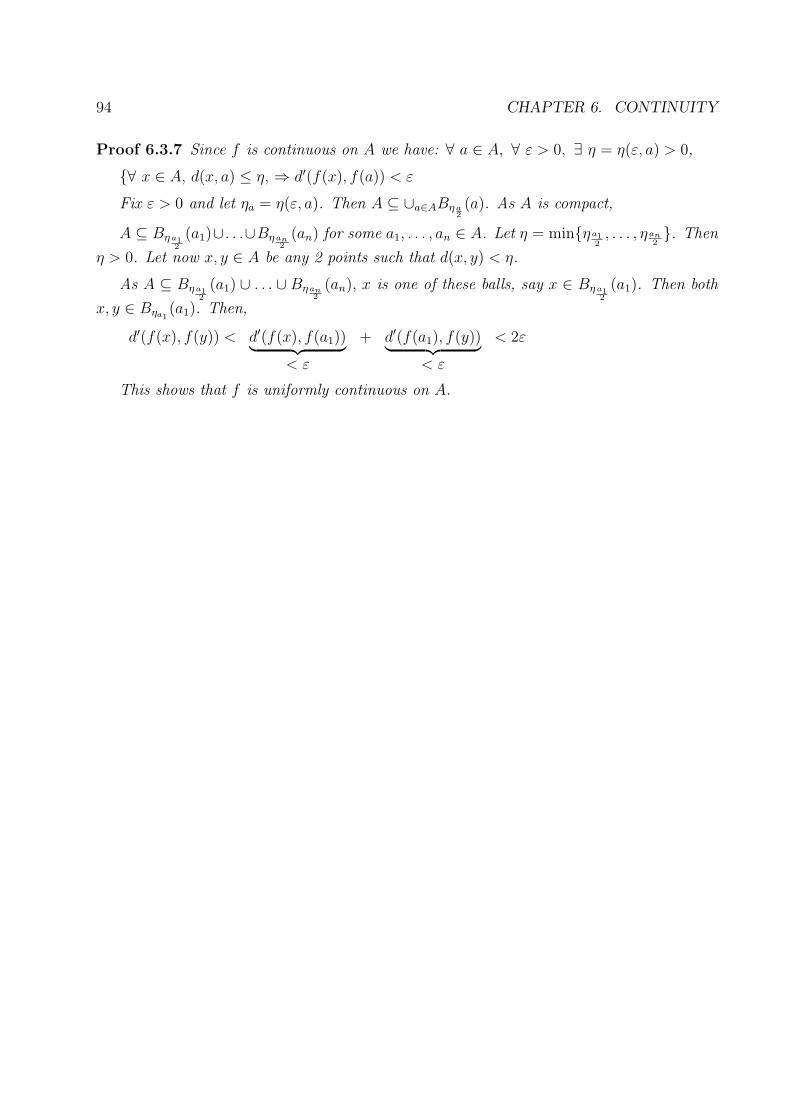
94 CHAPTER 6. CONTINUITY
Proof 6.3.7 Since f is continuous on A we have: ∀ a ∈ A, ∀ ε > 0, ∃ η = η(ε, a) > 0,
{∀ x ∈ A, d(x, a) ≤ η, ⇒ d′(f(x), f(a)) < ε
Fix ε > 0 and let ηa = η(ε, a). Then A ⊆ ∪a∈ABη a2(a). As A is compact,
A ⊆ Bη a12
(a1)∪ . . .∪Bη an2
(an) for some a1, . . . , an ∈ A. Let η = min{ηa12, . . . , η an
2}. Then
η > 0. Let now x, y ∈ A be any 2 points such that d(x, y) < η.
As A ⊆ Bη a12
(a1) ∪ . . . ∪ Bη an2
(an), x is one of these balls, say x ∈ Bη a12
(a1). Then both
x, y ∈ Bηa1(a1). Then,
d′(f(x), f(y)) < d′(f(x), f(a1))︸ ︷︷ ︸ + d′(f(a1), f(y))︸ ︷︷ ︸ < 2ε
< ε < ε
This shows that f is uniformly continuous on A.

6.3. UNIFORM CONTINUITY, LIPSCHITZEAN MAPPINGS 95
6.3.1 Exercises II
1. Let f : R → R be defined as f(x) =
⎧⎪⎪⎨⎪⎪⎩
0 if x ∈ R\Q1 if x = 01
qif x ∈ p
qand (p, q) = 1
Show that f is continuous at every irrational number and discontinuous at every ra-tional number.
2. Is there a function f : R → R which is continuous at every rational number anddiscontinuous at every irrational number?
3. Let (X, d) be a m.s., f : X → R be a function and g : X → R is given by
g(x) =f(x)
1 + |f(x)| .Let x0 ∈ X be a point. Show that g is continuous at x0 iff f is continuous at x0.
4. Let X be any set and f : X → R be a one-to-one function. Put, for x, y ∈ X,
d(x, y) = |f(x) − f(y)|. Show that d is a metric on X and f is continuous for thismetric.
5. A function f : R → R is said to be periodic if there is a number p > 0 such thatf(x + p) = f(x) for all x ∈ R. Show that every periodic continuous function isuniformly continuous on R and is bounded on R.
6. Let (X, d) be a metric space, A ⊆ X a set and f : A → R be a function. Assume thatf is continuous at a point x0 ∈ A.
Show that there are δ > 0 and M > 0 such that |f(x)| ≤ M for every x ∈ Bδ(x0) ∩ A.
Thus every continuous function is locally bounded.
7. Let f : ]0, 1[ → R be defined by f(x) =
{0 if x is irrational
n if x =n
mand (m,n) = 1
Prove that f is unbounded on every open interval I ⊆ ]0, 1[.
Deduce from 6 that f is discontinuous at every x ∈ ]0, 1[
8. Prove that the function f(x) =√
x is uniformly continuous on [0,∞[ and Lipschitzeanon [a, +∞[ for each a > 0.
9. Let (X, d) be a m.s., A ⊆ X a set and f : A → R be a function which is uniformlycontinuous on A.
Show that if (xn)n∈N is a Cauchy sequence in A, then (f(xn))n∈N is Cauchy in R.

96 CHAPTER 6. CONTINUITY
6.4 Uniform Extension Theorem
Let f : A → Y be a continuous function and A ⊆ B ⊆ X be a set.
Problem: Can we extend f continuously to B i.e. given f : A → Y continuous, is there acontinuous function f : B → Y such that f = f on A?
Example 6.4.1 Let A = R\{0}, f(x) = sin 1x, f : A → R. Then f is continuous, and
∀x ∈ A, |f(x)| ≤ 1, but as we have seen that f has no continuous extension to R.
Theorem 6.4.2 (Uniform Extension Theorem) If (Y, d′) is complete and f : A → Yis uniformly continuous on A, then there exists a unique uniformly continuous function.f : A → Y that extends f .
Proof 6.4.3 Let x ∈ A be a point. We want to extend f continuously to x. How to definef : A → R at x?
Let xn ∈ A, xn → x. Since xn → x, (xn)n∈N is Cauchy. As f is uniformly continuouson A, (f(xn))n∈N is Cauchy. As (Y, d′) is complete, (f(xn))n∈N converges to some pointαx ∈ Y .
Let us see that αx does not depend on the sequence (xn)n∈N that converges to x. To seethis, let (yn)n∈N be another sequence in A that converges to x. Then for the same reasons asabove, (f(yn))n∈N also converges in Y to same βx ∈ Y .
Is αx = βx?Let (zn)n∈N be the mixture of ′′(xn)n∈N and (yn)′′n∈N i.e.
zn = x0 , y0, x1, y1, . . .↑ ↑ ↑ ↑z0 z1 z2 z3
Then zn ∈ A and zn → x. Then (f(zn))n∈N is Cauchy, so f(zn) → γx for some γx ∈ Y .As (f(xn))n∈N and (f(yn))n∈N are subsequences of (f(zn))n∈N αx = γx and βx = γx. Soαx = γx. In particular, if x ∈ A, and if we take x0 = x1 = . . . = xn = . . . = x, αx = f(x) =limn→∞f(xn).
So we define f : A → R as f(x) = limn→∞f(xn) for any sequence (xn)n∈N in A thatconverges to x ∈ A.
What we did above shows that f is well-defined on A. Moreover f(x) = f(x), ∀ x ∈ A.Hence f is an extension of f to A. Let us see that f is uniformly continuous on A. As f isuniformly continuous on A, we have:
∀ ε > 0, ∃ η > 0, ∀ x, y ∈ A, d(x, y) ≤ η =⇒ d′(f(x), f(y)) ≤ ε Eq 7.3
Let us see that the same η works for f .To see this, let x, y ∈ A be such that d(x, y) < η. Let xn, yn ∈ A : xn → x and yn → y.
Then, there is an N ∈ N such that for n ≥ N, d(xn, yn) < η, since d(xn, yn) → d(x, y).Then by Eq 7.3, d′(f(xn), f(yn)) < ε. As d(f(x), f(y)) = limn→∞d(f(xn), f(yn)) ≤ ε. Sothat f is uniformly continuous on A.

6.4. UNIFORM EXTENSION THEOREM 97
Uniqueness: If g : A → Y is another uniformly continuous function extending f , theng(x) = f(x) = f(x), ∀ x ∈ A. Hence if x ∈ A and xn ∈ A, with xn → x, theng(x) = limn→∞f(xn) = f(x). So f = g on A.
Example 6.4.4 Every uniformly continuous f : Q → R is the restriction of an uniformlycontinuous f : R → R.
Example 6.4.5 The function f(x) = sin 1x
is not uniformly continuous on R \ {0}.
Definition 6.4.6 • Let f : A → Y be a function. If there is a number k > 0 such that∀x, y ∈ A, d′(f(x), f(y)) ≤ kd(x, y), then we say that f is a Lipschitzean function on A.
• If 0 < k < 1 then f is said to be a contraction.• If d′(f(x), f(y)) = d(x, y) ∀x, y ∈ A, then f is said to be an isometry.
Example 6.4.7 Let f(x) = sin x, f : R → R. Then sin(x) − sin(y) = (x − y) cos(c) forsome c between x and y.
So, sin(x) − sin(y)| ≤ |x − y|. Hence f(x) = sin x is a Lipschitzean function.More generally, if f : [a, b] → R is differentiable and f ′ is bounded on [a, b], then f is
Lipschitzean.
Example 6.4.8 Let f :]0,∞[→]0,∞[, f(x) = x +1
x, then |f(x)− f(y)| < |x− y| for x �= y
Example 6.4.9 If f : A → Y is Lipschitzean, then f is uniformly continuous. Indeed, if
for some k > 0 d′(f(x), f(y)) ≤ kd(x, y), then ∀ε > 0, ∃ η =ε
k: ∀x, y ∈ A, d(x, y) < η ⇒
d′(f(x), f(y)) ≤ kd(x, y) ≤ εThe converse is false. The function f : [o,∞[ → [0,∞[ , f(x) =
√x f is uniformly
continuous but not Lipschitzean.
Theorem 6.4.10 (Banach Fixed Point Theorem): Let (X, d) be a complete m.s. andf : X → X be a contraction. Then ∠∃!x ∈ X such that f(x) = x.
Proof 6.4.11 Let x0 ∈ X be any point. Then put x1 = f(x0), x2 = f(x1), ..., xn = f(xn)In this way, we obtain a sequence xn. Let us see that this sequence is Cauchy.First, d(xn, xn−1) = d(f(xn−1), f(xn−2)) ≤ kd(xn−1, xn−2), where 0 < k < 1 is a constant
independent from xn’s.Hence d(xn, xn−1) ≤ kn−2d(x1, x0). Then,
d(xn+p, xn) ≤ d(xn+p, xn+p−1) + ... + d(xn+1, xn)
≤ (kn+p−2 + ... + kn−1)d(x1, x0) = kn−1d(x1, x0)[1 + k + ... + kp−1] = kn−1d(x1, x0)1 − kp
1 − k
≤ kn−1d(x1, x0)
1 − kAs 0 < k < 1, kn−1 → 0 as n → ∞. Hence d(xn+p, xn) → 0 for any p ∈ N as n → ∞.
This shows that xn is Cauchy. As our m.s. (X, d) is complete, xn converges to some x ∈ X.

98 CHAPTER 6. CONTINUITY
Now, f(xn−1) = xn and since f is Lipschitzean, f is continuous on X. As xn = f(xn−1),letting n → ∞, x = f(x).
Uniqueness: Suppose that, for some y ∈ X, y = f(y) too. If x �= y, then f(x) �= f(y).So d(x, y) = d(f(x), f(y)) ≤ kd(x, y). If x �= y, then d(x, y) �= 0, so 1 ≤ k. Contradiction,since 0 < k < 1.
Example 6.4.12 f(x) sin x, f : [0, 2π] → [0, π], f(0) = 0. So, x = 0 is a fixed point of f .
Example 6.4.13 f(x) = ex, f : R → R, then the equation ex = x has no solution. So, fhas no fixed point.
Application: Let X = C[0, 1] = the space of the continuous functions, f : [0, 1] → R, withthe supremum metric. d(f, g) = sup0≤x≤1|f(x) − g(x)|. The m.s. (X, d) is complete. Showthat C[0, 1] is closed in B[0, 1]. Let f : [0, 1] × R → R be a continuous function such that|F (t, x) − F (t, y)| ≤ k|x − y| ∀ x, y ∈ R since 0 < k < 1 independent from x, y and t.
Consider the differential equation:{y′(t) = F (t, y(t)) ,
y(0) = 0 .
Question: Is there a solution?
Theorem 6.4.14 The equation system above has a solution.
Proof 6.4.15 Let T : C[0, 1] → C[0, 1] be the mapping defined by T (y)(t) =∫ t
0F (s, y(s))ds.
Then, for y, z ∈ C[0, 1],
|T (y)(t) − T (z(t))| = | ∫ t
0F (s, y(s)) − F (s, z(s)ds| ≤
∫ t
0|F (s, y(s)) − F (s, z(s))|ds
≤ k∫ t
0|y(s) − z(s)|ds ≤
∫ 1
0|y(s) − z(s)|ds
≤ k sup0≤s≤1 |y(s) − z(s)| = kd(y, z)
Then, d(T (y), T (z)) ≤ kd(y, z)Hence by the Banach Fixed Point Theorem, T has a unique fixed point y, T (y)(t) = y(t).So y(t) =
∫ t
0F (s, y(s))ds, hence y′(t) = F (t, y(t)) and y(0) = 0
Theorem 6.4.16 (Brewer Fixed Point Theorem): Let B = {x ∈ Rn : ||x||2 ≤ 1} bethe closed unit ball of Rn. Then every continuous f from B to B has a fixed point.
6.4.1 The distance function
Let (X, d) be a m.s. A ⊆ X a nonempty set and for x ∈ X. Let d(x, y) = infy∈A d(x, y). Thisis by definition, the distance of the point x to the set A. In this way, we define a functionf : X → R, f(x) = d(x,A). We want to study the properties of the function f .
Proposition 6.4.17 Let x ∈ X be given. Then d(x,A) = 0 ⇔ x ∈ A(so that if x /∈ A, d(x,A) > 0)

6.4. UNIFORM EXTENSION THEOREM 99
Proof 6.4.18 Suppose first that x ∈ A, then ∃ xn ∈ A : xn → x. Nowd(x,A) = infy∈A(x, y) ≤ d(x, xn) ∀n ∈ N . Hence d(x,A) = 0 (let n → ∞)
Conversely, suppose infy∈A d(x, y) = 0, so ∀n ≥ 1, ∃ yn ∈ A, d(x, yn) <1
n. Hence
yn → x. So, x ∈ A.
Proposition 6.4.19 ∀x1, x2 ∈ X, |d(x1, A) − d(x2, A)| ≤ d(x1, x2) (so f(x) = d(x,A) is aLipschitzean function on X.)
Proof 6.4.20 For any y ∈ A, d(x1, y) ≤ d(x1, x2) + d(x2, y) so thatinfy∈A d(x, y) ≤ d(x1, x2) + inf d(y2, x2) =⇒ d(x1, A) ≤ d(x1, x2) + d(x2, A).Hence, d(x1, A) − d(x2, A) ≤ d(x1, x2).Changing x1 and x2, we get d(x2, A) − d(x1, A) ≤ d(x1, x2).
Proposition 6.4.21 If A is compact, then ∀x ∈ A, there is a y0 ∈ A, d(x,A) = d(x, y0).
Proof 6.4.22 Let f : A → R, f(y) = d(x, y), f is continuous on X. Hence if A is compact,f attains its maximum on A, i.e. ∃ y0 ∈ A : f(y0) = infy∈A d(x, y), i.e. d(x, y0) = d(x,A).
6.4.2 Distance Between Two Points
Let (X, d) be a m.s. A,B be 2 nonempty sets. We define the distance between two setsd(A,B) as d(A,B) = infx∈B d(x,A) = infy∈A, x∈B d(x, y)
Example 6.4.23 Even if A, B are closed and disjoint, we may have d(A,B) = 0.Let X = R2, d = the Euclidean metric, A = {(x, 1
x) : x > 0} and B = R \ {0}. Then
A,B are closed and disjoint and d(A,B) = inf{√(x − a)2 + ( 1x− 0)2 : x > 0, a ∈ R}. Then
d(A,B) ≤ d((n, 1n), (n, 0)) =
1
n, ∀n > 0. This being true for each n, we get d(A, B) = 0.
However,
Theorem 6.4.24 If A is compact, B is closed and A ∩ B = ∅, then d(A,B) > 0.
Proof 6.4.25 Let f : A → R, f(x) = d(x,B). This is a continuous function. By theProposition 6.4.21, d(x,B) > 0, ∀x ∈ A. As A is compact f attains its minimum: ∃ x0 ∈A f(x0) = infx∈A d(x,B) = d(A,B). So, d(A,B) = f(x0) = d(x0, B) > 0.
Example 6.4.26 We use this proposition in the following form:Let O ⊆ X be an open set and K ⊆ O be a compact set. Then d(K, δO) > 0.e.g. Let X = R2, let O = B1(0), K ⊆ O be any compact set. Show that for some
0 < r < 1, K ⊆ Br(0).

100 CHAPTER 6. CONTINUITY
Example 6.4.27 f : R → R be the Dirichlet function f(x) =
{1 if x ∈ Q,
0 otherwise.
f is continuous iff ∀x0 ∈ R,∀xn ∈ R, xn → x0 ⇒ f(xn → f(x0)).So this function is not continuous as f |Q = 1 and f |R\Q = 0
Lemma 6.4.28 (Urysohn Lemma): Let (X, d) be any m.s., A,B 2 nonempty disjointsets. Then ∃ a function f : X → R, continuous such that;
1. ∀x ∈ X, 0 ≤ f(x) ≤ 1.
2. ∀x ∈ A, f(x) = 0.
3. ∀x ∈ B, f(x) = 1.
Proof 6.4.29 For x ∈ X, let f(x) =d(x,A)
d(x,A) + d(x,B)As A∩B = ∅ and A,B are closed d(x,A)+d(x,B) �= 0,∀x ∈ X. Hence f is continuous on
R, as the quotient of two continuous functions is continuous provided that the denominatoris not zero.
It is clear that 0 ≤ f(x) ≤ 1, for x ∈ A, f(x) = 0 and for x ∈ B, f(x) = 1.
6.4.3 Fσ-sets, Gδ-sets in R
Consider the sets [a, b], (a, b), one is closed and the other is open set. And we can write themas:
[a, b] = ∩n≥1]a − 1n, b + 1
n[ , and (a, b) = ∪n≥1[a + 1
n, b − 1
n]
Questions:
1. Can we write every closed set as a union of countable open sets?
2. Can we write every open set as a union of countable closed sets?
Definition 6.4.30 Let (X, d) be a m.s. and E ⊆ X a set. We say that;
1. E is a Gδ-set, if it is possible to write E as the intersection of countably many opensets. (i.e. E = ∩n∈NOn, On open)
2. E is said to be a Fσ-set, if it is possible to write E as the union of countably manyclosed sets. (i.e. E = ∪n∈NFn, Fn closed.)
Obviously,
1. E is a Gδ-set ⇔ Ec is an Fδ-set
2. Every open set O is a Gδ-set

6.4. UNIFORM EXTENSION THEOREM 101
3. Every closed set F is a Fδ-set
4. Every countable subset E ⊆ X is a Fδ-set. So Ec is a Gδ-set.
Notation: Let (X, d) be a m.s. A ⊆ X (�= ∅) any set and ε > 0. LetBε(A) = {x ∈ X : d(x,A) < ε}B′
ε(A) = {x ∈ X : d(x,A) ≤ ε}As the function f : X → R, f(x) = d(x,A) is continuous, Bε(A) = f−1(]−∞, ε[) is open
and B′ε(A) = f−1(]−∞, ε]) is closed. Also A ⊆ Bε(A) ⊆ B′
ε(A). If, in R, we take, A = [a, b]and ε = 1
n, then B 1
n(A) = {x ∈ R : d(x,A) < 1
n} =]a − 1
n, b + 1
n[.
Theorem 6.4.31 a) If A ⊆ X is closed, then A = ∩n≥1B 1n(A)
b) If A ⊆ X is open, then A = ∪n≥1(B 1n(Ac))c
Proof 6.4.32 It is enough to prove a.(a)(⇒) The inclusion A ⊆ ∩n≥1B 1
n(A) is clear.
(⇐) Let x /∈ A. As A is closed, there is some ε > 0 such that Bε(x)∩A = ∅. In particular,d(x,A) ≥ ε. If 1
n< ε, then x /∈ B 1
n(A). Hence x /∈ ∩n≥1B 1
n(A). Hence A = ∩n≥1B 1
n(A).
Conclusion: In any m.s. (X, d)a) Every closed set can be written as an intersection of countably many open sets.(Gδ-set)b) Every open set can be written as an union of countably many closed sets.(Fσ-set)
Question: In R, we have seen that Q is an Fσ-set and R \ Q is Gδ-set. Is Q a Gδ-set? i.e.is it possible to write Q as Q = ∩n≥1On, On ⊆ R open.
This is not the case.
Remark: Let f be any function. (f : R → R). Let Cf = {x ∈ R : f is continuous at x}.If f(x) = sin x, then Cf = R.If f(x) = χQ, then Cf = ∅.If f(x) = sin 1
x, then Cf = R \ {0}.
Now let f(x) =
⎧⎪⎨⎪⎩
0 if x ∈ R \ Q,
0 if x = 0,1m
if x = nm
and x ∈ Q (n,m) = 1
Let x0 ∈ R be a given point. Then f is continuous at x0 ⇔ x0 ∈ R \ Q i.e. Cf = R \ Q
Question: Is there a function f : R → R such that Cf = Q?
Theorem 6.4.33 Let A ⊆ R be a set (�= ∅). Then there is a function f : R → R such thatCf = A iff A is a Gδ-set.
So, since Q is not a Gδ-set, there is no function f : R → R which is continuous at everyrational x0, and discontinuous at every irrational x0.
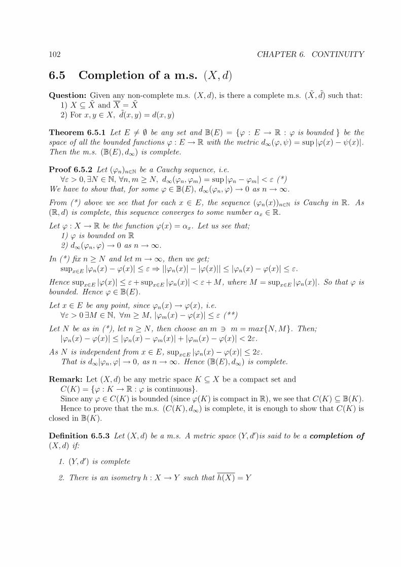
102 CHAPTER 6. CONTINUITY
6.5 Completion of a m.s. (X, d)
Question: Given any non-complete m.s. (X, d), is there a complete m.s. (X, d) such that:1) X ⊆ X and X = X2) For x, y ∈ X, d(x, y) = d(x, y)
Theorem 6.5.1 Let E �= ∅ be any set and B(E) = {ϕ : E → R : ϕ is bounded } be thespace of all the bounded functions ϕ : E → R with the metric d∞(ϕ, ψ) = sup |ϕ(x) − ψ(x)|.Then the m.s. (B(E), d∞) is complete.
Proof 6.5.2 Let (ϕn)n∈N be a Cauchy sequence, i.e.∀ε > 0, ∃N ∈ N, ∀n,m ≥ N, d∞(ϕn, ϕm) = sup |ϕn − ϕm| < ε (*)
We have to show that, for some ϕ ∈ B(E), d∞(ϕn, ϕ) → 0 as n → ∞.
From (*) above we see that for each x ∈ E, the sequence (ϕn(x))n∈N is Cauchy in R. As(R, d) is complete, this sequence converges to some number αx ∈ R.
Let ϕ : X → R be the function ϕ(x) = αx. Let us see that;1) ϕ is bounded on R2) d∞(ϕn, ϕ) → 0 as n → ∞.
In (*) fix n ≥ N and let m → ∞, then we get;supx∈E |ϕn(x) − ϕ(x)| ≤ ε ⇒ ||ϕn(x)| − |ϕ(x)|| ≤ |ϕn(x) − ϕ(x)| ≤ ε.
Hence supx∈E |ϕ(x)| ≤ ε + supx∈E |ϕn(x)| < ε + M , where M = supx∈E |ϕn(x)|. So that ϕ isbounded. Hence ϕ ∈ B(E).
Let x ∈ E be any point, since ϕn(x) → ϕ(x), i.e.∀ε > 0 ∃M ∈ N, ∀m ≥ M, |ϕm(x) − ϕ(x)| ≤ ε (**)
Let N be as in (*), let n ≥ N , then choose an m m = max{N,M}. Then;|ϕn(x) − ϕ(x)| ≤ |ϕn(x) − ϕm(x)| + |ϕm(x) − ϕ(x)| < 2ε.
As N is independent from x ∈ E, supx∈E |ϕn(x) − ϕ(x)| ≤ 2ε.That is d∞|ϕn, ϕ| → 0, as n → ∞. Hence (B(E), d∞) is complete.
Remark: Let (X, d) be any metric space K ⊆ X be a compact set andC(K) = {ϕ : K → R : ϕ is continuous}.Since any ϕ ∈ C(K) is bounded (since ϕ(K) is compact in R), we see that C(K) ⊆ B(K).Hence to prove that the m.s. (C(K), d∞) is complete, it is enough to show that C(K) is
closed in B(K).
Definition 6.5.3 Let (X, d) be a m.s. A metric space (Y, d′)is said to be a completion of(X, d) if:
1. (Y, d′) is complete
2. There is an isometry h : X → Y such that h(X) = Y

6.5. COMPLETION OF A M.S. (X, D) 103
Example 6.5.4 Consider X = Q, d(x, y) = |x − y|. Then j : Q → R, j(x) = x X = R,d(x, y) = |x − y| and j(Q) = R.
(Q, d) is not complete but (Q, d), i.e. (R, d) is complete.
Let (X, d) be any m.s. We are going to show that there is a complete m.s. (X, d) and anisometry j : X → X such that j(X) = X
Theorem 6.5.5 Given any m.s. (X, d), there is a complete m.s. (X, d) and an isometryj : X → X such that j(X) = X. The space (X, d) is unique up to an isometry.
Proof 6.5.6 Let B(X) = {f : X → R : f is bounded} be the space of bounded functionswith the metric d∞(f, g) = supx∈X |f(x) − g(x)|. We know that (B(X), d∞) is a completem.s.
Now, fix a point a ∈ X. For any y ∈ X, let fy : X → R be the function defined byfy(x) = d(a, x) − d(x, y). Then |fy(x)| = |d(a, x) − d(x, y)| ≤ d(a, y). So, fy is bounded onX. So, fy ∈ B(X).
Let j : X → B(X) be defined j(y) = fy. j is an isometry i.e. d∞(fy, fy′) = d(y, y′) i.e.supx∈X |fy(x) − fy′(x)| = d(y, y′), since
|fy(x) − fy′(x)| = |d(a, x) − d(x, y) − d(a, x) + d(x, y′)| = |d(x, y) − d(x, y′)| ≤ d(y, y′).
Hence sup |fy(x) − fy′(x)| ≤ d(y, y′). Then for y = y′, |fy(x) − fy′(x)| = d(y, y′). Hence
sup |fy(x) − fy′(x)| = d(y, y′). So, j : X → B(X) is an isometry. Let X = j(X) and d = d′
on X. Then (X, d) is a complete m.s. and j(X) = X.
Note that: In any complete m.s. (Y, d), if M ⊆ Y closed, then (M,d) is complete.
Uniqueness: Let (Y , d) be another complete metric space and i : X → Y an isometry withi(X) = Y . In i : X → Y consider X as a subspace of X. In j : X → X consider X asa subspace of Y . Then i has a uniformly continuous extension i∗ : X → Y . And j has auniformly continuous extension j∗ : Y → X.
Both i∗ and j∗ are isometries: i∗ ◦ j∗ : Y → Y is an identity on Y .
Example 6.5.7 Let X = C00 with the metric d∞(x, y) = supn∈N|xn − yn| where the spaceis:
C00 = {ϕ : N → R : ϕ is almost finite}= {ϕ : ϕ(n) = xn = 0 for all but finitely many n ∈ N}
Let X = C0 = {ϕ : N → R : limn→∞ ϕ(n) = 0} with the supremum metric. Then:(C0, d∞) is complete, C00 ⊆ C0 and C00 = C0 as j : X → X, j(x) = x is an isometry.
6.5.1 Equivalence of Metrics
Let (X, d1) be a m.s. and d2 be another metric on X.Question: If we place d1 by d2, what we gain, what we loose?

104 CHAPTER 6. CONTINUITY
Example 6.5.8 Let on define the metrics; d(x, y) = |x − y|, d1(x, y) = |x3 − y2|d2(x, y) = |Arc tan x − Arc tan y|, d3(x, y) =
|x − y|1 + |x − y|
For all these metrics, |xn − x| → 0 ⇔ di(xn, x) → 0 is the same.But being bounded change;Let xn = n then d2(xn, xm) = |Arc tan xn − Arc tan xm| → 0 as n,m → ∞, so it is
Cauchy for this metric, but not Cauchy for d for example.
Let f : (X, d1) → (X, d2) be identity mapping f(x) = x. Then;
1) f is continuous iff whenever d1(xn, x) → 0 we have d2(xn, x) → 0.2) f is a homeomorphism iff d1(xn, x) → 0 ⇔ d1(xn, x) → 0
Definition 6.5.9 A property (p) on a m.s. (X, d) is said to be topological property ifit is definable in terms of open sets e.g. to be compact, separable,closed sets, convergentsequences...
Definition 6.5.10 There are 3 types of equivalences:a) d1 and d2 are topologically equivalent if f is a homeomorphism. (i.e. f and f−1 are
both continuous) In this, for any sequence xn ∈ X and x ∈ X d1(xn, x) → 0 ⇔ d2(xn, x) → 0.So, in this case, the spaces (X, d1), (X, d2) have the same topological properties. Thus,
if we replace d by a topological equivalent metric d2, then we do not lose any topologicalproperty, but we may lose non-topological properties such as completeness.
b) d1 and d2 are uniformly equivalent if both f and f−1 are uniformly continuous. Ifd1, d2 are uniformly equivalent then they are topologically equivalent. If we replace a metricd1 by a uniformly equivalent metric d2, then we do not lose any topological properties, we donot lose completeness, but it may happen that a set A ⊆ X which is bounded for d1, is notbounded for d2, vice versa.
c) d1 and d2 are said to be equivalent if both f and f−1 are Lipschitzean. That is d1
and d2 are equivalent ⇔ ∃ α > 0, β > 0 : αd1(x, y) ≤ d2(x, y) ≤ βd1(x, y) ∀ x, y ∈ X. If wereplace a metric d1 by an equivalent metric d2 we lose almost nothing. However a functionf : X → X may be a contraction with respect to one of these metric but not w.r.t. othermetric.
Example 6.5.11 Let X = R, d1(x, y) = |x − y|, d2(x, y) = |Arc tan x − Arc tan y|. Thenfor any xn ∈ X and x ∈ X, |xn − x| → 0 ⇔ |Arc tan x − Arc tan y| → 0. So that d1, d2 aretopologically equivalent. But (R, d1) is complete, (R, d2) is not complete.
Example 6.5.12 Let X = R, d1(x, y) = |x − y|, d2(x, y) = min{1, |x − y|} ≤ 1. Then forxn ∈ R, x ∈ R. d1(xn, x) → 0 ⇔ d2(xn, x) → 0. Hence d1, d2 are topologically equivalent. Ris not bounded for d1, but R is bounded for d2.
Example 6.5.13 Let X = R, d1(x, y) = |x− y|, d2(x, y) = min{1, |x− y|}. Then d1 and d2
are uniformly equivalent. A sequence (xn)n∈N in R which is Cauchy w.r.t. d1 iff it is Cauchyw.r.t. d2. But the spaces (R, d1) and (R, d2) do not have the same bounded sets.

6.5. COMPLETION OF A M.S. (X, D) 105
Example 6.5.14 Let X = Rn, then any 2 of the metrics (dp)1≤p≤∞ are equivalent.But B1(0) for d∞, B1(0) for d2 and B1(0) for d1 are different geometrically.

106 CHAPTER 6. CONTINUITY

Chapter 7
Limit
1. Definition and Existence of Limit
2. Limit from the left, from the right
3. Continuity of Monotone functions
4. Functions of Bounded Variation
5. Absolutely Continuous Functions
In this chapter, we will work in the following setting:
(X, d), (Y, d′) are 2 m.s., A ⊆ X a set, a ∈ A a point, and f : A → Y a function. The pointa may or may not be in A and f need not to be defined at the point a.
7.1 Definition and Existence of Limit
Definition 7.1.1 We say that limx→a f(x) exists if;∃ L ∈ Y such that ∀ ε > 0, ∃ η > 0, ∀x ∈ A ∩ Bη(a) : d′(f(x), L) < ε.
In this case we write L = limx→a, x∈A f(x) (=limit of f(x) as x goes to a while remaining inthe set A). Then, the set A “determines” the way x goes to a.
Example 7.1.2 Let X = Y = R, A =]−1, 0[∪]0, 1[, a = 0 (So, a ∈ A, but also 0 ∈ ] − 1, 0[and 0 ∈ ]0, 1[)
Let f : A → R, f(x) =
{−1 if x ∈] − 1, 0[,
1 if x ∈]0, 1[.
Then, limx→0, x∈A f(x) does not exist. Indeed, otherwise we would have some L ∈ Rsatisfying the definition of limit: ∀ ε > 0, ∃ η > 0 : ∀ x ∈] − η, η [∩A =⇒ |f(x) − L| < ε
Let x ∈]− η, η [∩A, x > 0. Then f(x) = 1, so |1−L| < ε. Then, let x ∈ ]− η, η [∩A, x < 0.Then f(x) = −1, so | − 1 − L| < ε. So, for ε = 1
2, this is not possible.
Now, if we take A =]0, 1[ then limx→0, x∈A f(x) = 1. So, existence depends on the set.
107
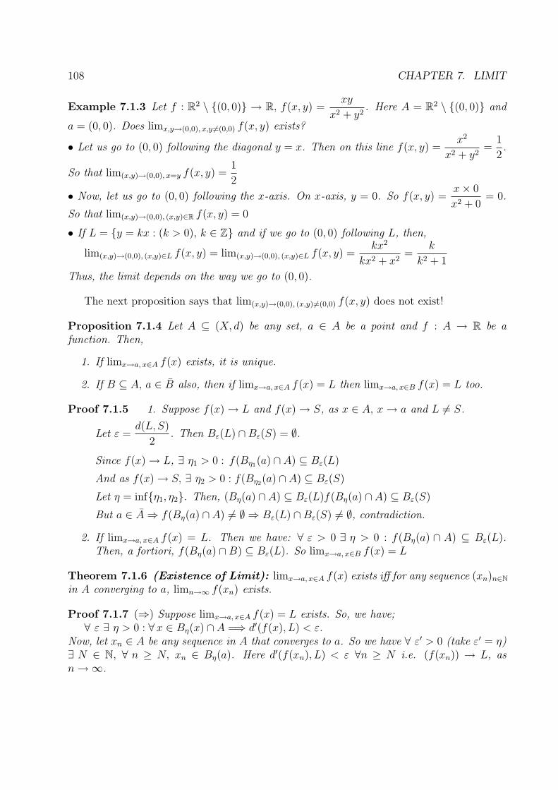
108 CHAPTER 7. LIMIT
Example 7.1.3 Let f : R2 \ {(0, 0)} → R, f(x, y) =xy
x2 + y2. Here A = R2 \ {(0, 0)} and
a = (0, 0). Does limx,y→(0,0), x,y �=(0,0) f(x, y) exists?
• Let us go to (0, 0) following the diagonal y = x. Then on this line f(x, y) =x2
x2 + y2=
1
2.
So that lim(x,y)→(0,0), x=y f(x, y) =1
2
• Now, let us go to (0, 0) following the x-axis. On x-axis, y = 0. So f(x, y) =x × 0
x2 + 0= 0.
So that lim(x,y)→(0,0), (x,y)∈R f(x, y) = 0
• If L = {y = kx : (k > 0), k ∈ Z} and if we go to (0, 0) following L, then,
lim(x,y)→(0,0), (x,y)∈L f(x, y) = lim(x,y)→(0,0), (x,y)∈L f(x, y) =kx2
kx2 + x2=
k
k2 + 1
Thus, the limit depends on the way we go to (0, 0).
The next proposition says that lim(x,y)→(0,0), (x,y) �=(0,0) f(x, y) does not exist!
Proposition 7.1.4 Let A ⊆ (X, d) be any set, a ∈ A be a point and f : A → R be afunction. Then,
1. If limx→a, x∈A f(x) exists, it is unique.
2. If B ⊆ A, a ∈ B also, then if limx→a, x∈A f(x) = L then limx→a, x∈B f(x) = L too.
Proof 7.1.5 1. Suppose f(x) → L and f(x) → S, as x ∈ A, x → a and L �= S.
Let ε =d(L, S)
2. Then Bε(L) ∩ Bε(S) = ∅.
Since f(x) → L, ∃ η1 > 0 : f(Bη1(a) ∩ A) ⊆ Bε(L)
And as f(x) → S, ∃ η2 > 0 : f(Bη2(a) ∩ A) ⊆ Bε(S)
Let η = inf{η1, η2}. Then, (Bη(a) ∩ A) ⊆ Bε(L)f(Bη(a) ∩ A) ⊆ Bε(S)
But a ∈ A ⇒ f(Bη(a) ∩ A) �= ∅ ⇒ Bε(L) ∩ Bε(S) �= ∅, contradiction.
2. If limx→a, x∈A f(x) = L. Then we have: ∀ ε > 0 ∃ η > 0 : f(Bη(a) ∩ A) ⊆ Bε(L).Then, a fortiori, f(Bη(a) ∩ B) ⊆ Bε(L). So limx→a, x∈B f(x) = L
Theorem 7.1.6 (Existence of Limit): limx→a, x∈A f(x) exists iff for any sequence (xn)n∈N
in A converging to a, limn→∞ f(xn) exists.
Proof 7.1.7 (⇒) Suppose limx→a, x∈A f(x) = L exists. So, we have;∀ ε ∃ η > 0 : ∀x ∈ Bη(x) ∩ A =⇒ d′(f(x), L) < ε.
Now, let xn ∈ A be any sequence in A that converges to a. So we have ∀ ε′ > 0 (take ε′ = η)∃ N ∈ N, ∀ n ≥ N, xn ∈ Bη(a). Here d′(f(xn), L) < ε ∀n ≥ N i.e. (f(xn)) → L, asn → ∞.

7.1. DEFINITION AND EXISTENCE OF LIMIT 109
(⇐) Conversely, suppose that, for any sequence (xn)n∈N in A converging to a limn→∞ f(xn)exists.
Let us first see that if xn ∈ A, with xn → a; and yn ∈ A with yn → a, then we havelimn→∞ f(xn) = limn→∞ f(yn). To see this let L1 = limn→∞ f(xn), L2 = limn→∞ f(yn).Then mix up the sequences (xn)n∈N and (yn)n∈N to get a sequence (zn)n∈N as follows:
x0, y0, x1, y1, x2, y2, ..., xn, yn, ...
Then zn ∈ A and zn → a too. So, L3 = limn→∞ f(zn) exists. As (f(xn))n∈N and (f(yn))n∈N
are subsequences of (f(zn))n∈N L1 = L2 = L3. Hence limn→∞ f(xn) does not depend on thesequence (xn)n∈N chosen.
Now, let (xn)n∈N be any sequence in A that converges to a. Then let L = limn→∞ f(xn). Letus see that limx→a, x∈A f(x) = L. If not, we would have: ∃ ε > 0 ∀ η > 0 : ∃ xη ∈ Bη(a)∩A :d′(f(xη), L) ≥ ε. Let η = 1
nand denote by xn the corresponding xη. Then xn ∈ B 1
n(a) ∩ A.
So xn ∈ A and xn → a.
Hence limn→∞ f(xn) = L but d′(f(xn), L) ≥ ε ∀n ≥ 1, contradiction.So limx→a, x∈A f(x) = L.
Proposition 7.1.8 Let f, g : A → R be two functions. Suppose that limx→x0, x∈A f(x) andlimx→x0, x∈A g(x) exists. Then;
1. limx→x0, x∈A(f(x) + g(x)) exists and is equal to limx→x0, x∈A f(x) + limx→x0, x∈A g(x)
2. limx→x0, x∈A(f(x)g(x)) exists and is equal to limx→x0, x∈A f(x) limx→x0, x∈A g(x)
3. If g(x) �= 0 and limx→x0, x∈A g(x) �= 0, then limx→x0, x∈Af(x)
g(x)=
limx→x0, x∈A f(x)
limx→x0, x∈A g(x)
7.1.1 Cauchy Condition For Limit
Let f : A → Y be a function. We say that f satisfies the Cauchy Condition at a if wehave: ∀ ε > 0 ∃ η > 0 ∀ x, y ∈ Bη(a) ∩ A, d′(f(x), f(y)) < ε
Theorem 7.1.9 Suppose that (Y, d′) is complete. Then limx→a, x∈A f(x) = L exists iff fsatisfies the Cauchy condition at a.
Proof 7.1.10 (⇒) Suppose limx→a, x∈A f(x) = L exists. So, we have: ∀ ε > 0 ∃ η > 0 :
∀ x ∈ Bη(a) ∩ A ⇒ d′(f(x), L) <ε
2. Then, ∀ x, y ∈ Bη(a),
d′(f(x), f(y)) ≤ d′(f(x), L) + d′(f(y), L) < ε.
(⇐) Conversely, suppose f satisfies the Cauchy condition at a. Then,∀ ε > 0 ∃ η > 0 ∀ x, y ∈ Bη(a) ∩ A : d′(f(x), f(y)) < ε
Now, let (xn)n∈N be a sequence in A that converges to a. Then (for ε = η) there is N ∈ Nsuch that ∀ n ≥ N, d(xn, a) < η. So, ∀ n ≥ N, ∀ m ≥ N, xn, xm ∈ Bη(a) ∩ A. Henced′(f(xn), f(xm)) < ε. So, (f(xn))n∈N is Cauchy. As (Y, d′) is complete, limn→∞ f(xn) exists.
Hence by the Theorem 7.1.6, limx→a, x∈A f(x) = L exists.

110 CHAPTER 7. LIMIT
Example 7.1.11 Let Y = R, f : A → R be a function and M > 0 a number such that∀x, y ∈ A, |f(x) − f(y)| ≤ Md(x, y). For x0 ∈ A show that limx→x0, x∈A f(x) exists. Let ussee that Cauchy condition is satisfied:
Let ε > 0 be any given number, let 0 < η ≤ ε
2M, then ∀x, y ∈ A ∩ Bη(x0),
|f(x) − f(y)| ≤ Md(x, y) ≤ M [d(x, x0) + d(y, x0)] ≤ M(ε
2M+
ε
2M) = ε
So f satisfies Cauchy condition at x0, hence the limit exists.
Here we can even determine the limit. Indeed, the condition given for the function aboveimplies that f is uniformly continuous on A. Hence by the ‘Extension by the Uniform Conti-nuity theorem’ we can extend f continuously to a function f ∗ : A → R. As f ∗ is continuouson A and x0 ∈ A, for any sequence xn ∈ A converging to x0, limn→∞ f(xn) = f∗(x0). HenceL = f ∗(x0) is the limit of f as x → x0, x ∈ A.
7.1.2 Limit and continuity
Theorem 7.1.12 Suppose that a ∈ A (so that f is defined at a). Then f : A → Y iscontinuous at a iff limx→a, x∈A f(x) = f(a).
Proof 7.1.13 (⇒) Suppose f is continuous at a. Then, for any sequence (xn) that converg-ing to a, f(xn) → f(a). So, by the theorem 7.1.6, limx→a, x∈A f(x) = f(a).
(⇐) Suppose that limx→a, x∈A f(x) = f(a). Then, again by the same theorem, for anysequence (xn)n∈N in A converging to a, f(xn) → f(a). So f is continuous at a.
7.2 Limit From the Left, From the Right
First, a general result:
Lemma 7.2.1 Suppose that A = B ∪ C for B, C ⊆ X and x0 ∈ B, x0 ∈ C. Thenlimx→x0, x∈A f(x) exists iff both limx→x0, x∈B f(x) and limx→x0, x∈C f(x) exist and they arethe same.
Proof 7.2.2 (⇒) Suppose that limx→a, x∈A f(x) exists and is L. So, we have:∀ ε > 0, ∃ η > 0, ∀ x ∈ Bη(a) ∩ A: d′(f(x), L) < ε.
Then, obviously ∀ x ∈ Bη(a) ∩ B, d′(f(x), L) < ε, so limx→a, x∈B f(x) = L and similarly∀ x ∈ Bη(a) ∩ B, d′(f(x), L) < ε, so limx→a, x∈C f(x) = L.
(⇐) Conversely, suppose that this two limits exist and they are the same. Let L be thecommon value of these. So we have:
∀ε > 0, ∃η1 > 0 : ∀x ∈ B ∩ Bη1(x0), d′(f(x), L) < ε∀ε > 0, ∃η2 > 0 : ∀x ∈ C ∩ Bη2(x0), d′(f(x), L) < εLet η = min{η1, η2} then ∀x ∈ A ∩ Bη(X0), d′(f(x), L) < ε.Hence limx→x0, x∈A f(x) = L.

7.2. LIMIT FROM THE LEFT, FROM THE RIGHT 111
Now, in this section our X = R, d=usual metric. And let A = [b, a[∪]a, c] with B = [b, a[and C =]a, c]. We see that a ∈ A, a ∈ B and a ∈ C.So, for f : A → Y, limx→a, x∈A f(x), limx→a, x∈B f(x), and limx→a x ∈ Cf(x) are meaningful.The Lemma 7.2.1 says that:
limx→a, x∈A f(x) exists ⇔ limx→a, x∈B f(x) and limx→a, x∈C f(x) exists and are equal.
limx→a, x∈B f(x) is said to be the limit from the left and is denoted as limx→a, x<a f(x).
limx→a, x∈C f(x) is said to be the limit from the right and is denoted as limx→a, x>a f(x).
Mathematically:limx→a, x<a f(x) = L ⇔ ∀ ε > 0 ∃ η > 0 : ∀ x ∈]a − η, a[→ d′(f(x), L) < εlimx→a, x>a f(x) = L ⇔ ∀ ε > 0 ∃ η > 0 : ∀ x ∈]a, a + η[→ d′(f(x), L) < ε
Example 7.2.3 f : [−1, 0[∪]0, 1[→ R, f(x) =
{1 0 ≤ x ≤ 1,
−1 −1 ≤ x ≤ 0
limx→0, x<0 f(x) = −1 and limx→0, x>0 f(x) = 1
Notation: Now on we shall denote limx→x0, x<x0 f(x) as f(x−0 ) whenever this limit exists.
Similarly, we denote limx→x0, x>x0 f(x) as f(x+0 ) whenever this limit exists.
Example 7.2.4 Let f : [−π, 0[∪]0, π] → R, f(x) = sin 1x. Then neither of the limits
limx→x0, x<x0 f(x), limx→x0, x>x0 f(x) exist.
• If we take xn =1
π/2 + nπthen xn ∈]0, π] but limn→∞ f(xn) does not exist.
• If we take xn =−1
π/2 + nπthen xn ∈ [−π, 0[ but limn→∞ f(xn) does not exist.
Continuity From the Left, Continuity From the Right
Definition 7.2.5 Let b < a < c, f : [b, c] → Y be a function (So f is defined at a).• If limx→a, x<a f(x) = f(a), then we say f is continuous at a from left.• If limx→a x > af(x) = f(a), then we say f is continuous at a from right.
Example 7.2.6 Let f1, f2, f3 : [−1, 1] → R
1. f1(x) =
{−1 −1 ≤ x ≤ 0,
1 0 ≤ x ≤ 1As limx→0, x<0 f1(x) = −1 = f1(0), f is continuous at 0.
2. f2(x) =
{−1 −1 ≤ x ≤ 0,
1 0 ≤ x ≤ 1As limx→0, x>0 f2(x) = 1 = f2(0), f is continuous at 0.
3. f3(x) =
{−1 −1 ≤ x ≤ 0,
1 0 ≤ x ≤ 1limx→0, x<0 f3(x) = −1 �= f3(0) �= limx→0, x>0 f3(x), f is
not continuous neither from left, nor from right.
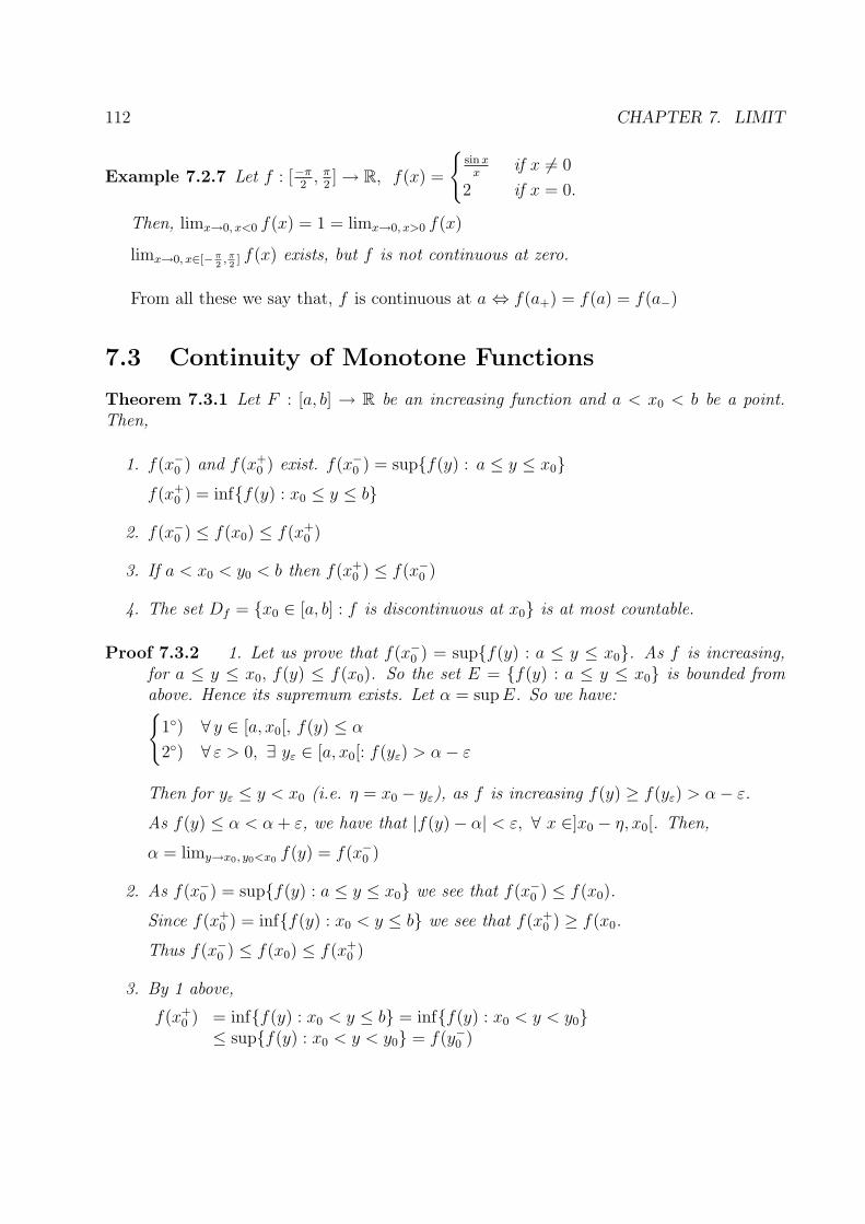
112 CHAPTER 7. LIMIT
Example 7.2.7 Let f : [−π2
, π2] → R, f(x) =
{sin x
xif x �= 0
2 if x = 0.
Then, limx→0, x<0 f(x) = 1 = limx→0, x>0 f(x)
limx→0, x∈[−π2
, π2] f(x) exists, but f is not continuous at zero.
From all these we say that, f is continuous at a ⇔ f(a+) = f(a) = f(a−)
7.3 Continuity of Monotone Functions
Theorem 7.3.1 Let F : [a, b] → R be an increasing function and a < x0 < b be a point.Then,
1. f(x−0 ) and f(x+
0 ) exist. f(x−0 ) = sup{f(y) : a ≤ y ≤ x0}
f(x+0 ) = inf{f(y) : x0 ≤ y ≤ b}
2. f(x−0 ) ≤ f(x0) ≤ f(x+
0 )
3. If a < x0 < y0 < b then f(x+0 ) ≤ f(x−
0 )
4. The set Df = {x0 ∈ [a, b] : f is discontinuous at x0} is at most countable.
Proof 7.3.2 1. Let us prove that f(x−0 ) = sup{f(y) : a ≤ y ≤ x0}. As f is increasing,
for a ≤ y ≤ x0, f(y) ≤ f(x0). So the set E = {f(y) : a ≤ y ≤ x0} is bounded fromabove. Hence its supremum exists. Let α = sup E. So we have:{
1◦) ∀ y ∈ [a, x0[, f(y) ≤ α
2◦) ∀ ε > 0, ∃ yε ∈ [a, x0[: f(yε) > α − ε
Then for yε ≤ y < x0 (i.e. η = x0 − yε), as f is increasing f(y) ≥ f(yε) > α − ε.
As f(y) ≤ α < α + ε, we have that |f(y) − α| < ε, ∀ x ∈]x0 − η, x0[. Then,
α = limy→x0, y0<x0 f(y) = f(x−0 )
2. As f(x−0 ) = sup{f(y) : a ≤ y ≤ x0} we see that f(x−
0 ) ≤ f(x0).
Since f(x+0 ) = inf{f(y) : x0 < y ≤ b} we see that f(x+
0 ) ≥ f(x0.
Thus f(x−0 ) ≤ f(x0) ≤ f(x+
0 )
3. By 1 above,
f(x+0 ) = inf{f(y) : x0 < y ≤ b} = inf{f(y) : x0 < y < y0}
≤ sup{f(y) : x0 < y < y0} = f(y−0 )

7.4. FUNCTIONS OF BOUNDED VARIATION 113
4. By 2 above, f is discontinuous at a point x0 ∈]a, b[⇔ f(x−0 ) < f(x+
0 ).
Now, let x0 < y0, x0, y0 ∈ Df . So, f(x−0 ) < f(x+
0 ) ≤ f(y−0 ) < f(y+
0 ). Let rx0 , ry0 ∈ Qbe such that f(x−
0 ) < rx0 < f(x+0 ) and f(y−
0 ) < ry0 < f(y+0 ). Then x0 < y0 ⇒ rx0 < ry0.
Then we can define a one-to-one mapping from Df into Q. As Q is countable, we canconclude that Df is countable.
7.4 Functions of Bounded Variation
Definition 7.4.1 Consider an interval [a, b]. A finite subset P = {x0, x1, ..., xn} of [a, b] issaid to be a partition of [a, b] if a = x0 < x1 < ... < xn = b.
Definition 7.4.2 Let f : [a, b] → R be any function. The quantity;
V (f, P ) =n∑
i=1
|f(xi) − f(xi−1)|is said to be the variation of f relative to the partition P .
Example 7.4.3 Suppose that f is an increasing function. Then,
V (f, p) =n∑
i=1
|f(xi) − f(xi−1)| =n∑
i=1
(f(xi) − f(xi−1)) = f(b) − f(a).
Definition 7.4.4 Let f : [a, b] → R be any function and P[a, b] be the set of all partitionsof [a, b]. Put V b
a (f) = supP∈P[a,b] V (f, P ). If V ba (f) < ∞ we say that f is a function of
bounded variation. (V ba (f) is the total variation of f on [a, b].)
Example 7.4.5 If f : [a, b] → R is increasing then V ba (f) ≤ f(b) − f(a) < ∞. Hence any
increasing function f : [a, b] → R is of bounded variation.
Example 7.4.6 Even if a function f : [a, b] → R is continuous, it need not to be of bounded
variation. Let f : [0, 1] → R, f(x) =
{x sin 1/x if x �= 0
0 if x = 0
Then f is continuous on [0, 1].
Now, let n ≥ 1 any number and P be a partition of [0, 1].
x0 = 0 < x1 =1
π + π/2< x2 =
1
2π + π/2< ... <
1
nπ + π/2< xn+1 = 1.
V (f, p) =n+1∑i=1
|f(xi) − f(xi−1)| Now,
114 CHAPTER 7. LIMIT
|f(xi) − f(xi−1)| = | 1
iπ + π/2sin(iπ + π/2) − 1
(i − 1)π + π/2sin((i − 1)π + π/2)|
= | 1
iπ + π/2(−1)i − 1
(i − 1)π + π/2(−1)i − 1|
=1
iπ + π/2+
1
(i − 1)π + π/2
≥ 1
iπ + π/2≥ 1
π(1 + i)
V (f, p) ≥ 1
π
n∑i=1
1
1 + i→ ∞, as n → ∞. Hence supp∈P[a,b] V (f, p) = ∞.
Remark: Every function of bounded variation, f : [a, b] → R is bounded.
Indeed, let x ∈]a, b[, let P = {a, x, b}, thenV (f, P ) = |f(a) − f(x)| + |f(x) − f(b)| ≤ V (f, [a, b]) < ∞.
Hence |f(x)| − |f(a)| + |f(x)| − |f(b)| ≤ V (f, [a, b])
⇒ |f(x)| ≤ 1
2[|f(a)| + |f(b)| + V (f, [a, b])], so that f is bounded.
Example 7.4.7 If f and g are of bounded variation then, f ± g and cf are of boundedvariation. Thus the space BV [a, b] of the functions f : [a, b] → R of bounded variation is avector space.
Lemma 7.4.8 Let f : [a, b] → R be a function of bounded variation and a < c < b benumbers. Then V (f, [a, b]) = V (f, [a, c]) + V (f, [c, b])
Proof 7.4.9 Let P = {x0, x1, ..., xn} be any partition of [a, b], then P = P ∪ {c} is also apartition of [a, b].
Moreover, V (f, P ) ≤ V (f, P ) since |f(xi) − f(xi+1)| ≤ |f(xi) − f(c)| + |f(c) − f(xi+1)|Let P1 = [a, c] ∩ P , P2 = [c, b] ∩ P , then P1 is a partition of [a, c], P2 is a partition of [c, b].
Now V (f, P ) = V (f, P1 ∪ P2) = V (f, P1) + V (f, P2) ≤ V (f, [a, c]) + V (f, [c, b])
Hence V (f, P ) ≤ V (f, [a, c]) + V (f, [c, b])
V (f, [a, b]) = supP∈P[a,b] V (f, P ) ≤ V (f, [a, c]) + V (f, [c, b])
To prove that the reverse inequality, let ε > 0 arbitrary. Then there are partitions P3, P4 of[a, c], [c, b] respectively, such that;
V (f, P3) > V (f, [a, c]) − ε/2 and V (f, P4) > V (f, [c, b]) − ε/2
Let P ′ = P3 ∪ P4 then P ′ is a partition of [a, b], so thenV (f, [a, b]) ≥ V (f, P ′) = V (f, P3) + V (f, P4) ≥ V (f, [a, c]) + V (f, [c, b]) − ε
Hence V (f, [a, b]) = V (f, [a, c]) + V (f, [c, b])
Theorem 7.4.10 (Characterization of the functions of bounded variation): Letf : [a, b] → R be a given function. Then f is of bounded variation iff f is the difference oftwo increasing functions, i.e. f = f1 − f2, where f1, f2 are increasing functions.

7.5. ABSOLUTELY CONTINUOUS FUNCTIONS 115
Proof 7.4.11 (⇐) If f = f1 − f2, then for any partition P of [a, b], V (f, p) ≤ V (f1, p) +V (f2, p) ≤ f1(b) − f2(a). So that V b
a (f) < ∞.
(⇒) Conversely, suppose V ba (f) < ∞. Let, for a ≤ x ≤ b, g(x) = V x
a (f). It is clear that g isincreasing. Now let h(x) = V x
a (f) − f(x). Let us see that h is increasing:
Let 0 ≤ x ≤ y be two points. Then h(y) − h(x) = V ya (f) − V x
a (f) − [f(y) − f(x)]. Now,V y
a (f) − V xa (f) ≥ |f(y) − f(x)|. Hence h(y) − h(x) ≥ 0.
So h is increasing and f(x) = g(x) − h(x).
Example 7.4.12 If f : [a, b] → R is differentiable and f ′ is bounded on [a, b] then V ba (f) <
∞. Indeed, let P = {x0, x1, ..., xn} be any partition of [a, b]. Since by the intermediate valuetheorem, f(xi) − f(xi−1) = (xi − xi−1)f
′(ci) for some xi−1 < ci < xi.
If |f ′(x)| < M ∀x ∈ [a, b], then;
V (f, p) =n+1∑i=1
|f(xi) − f(xi−1)| ≤n+1∑i=1
(xi − xi−1)|f ′(ci)| ≤ M
n+1∑i=1
(xi − xi−1) = M(b − a).
So, V ba (f) = supp∈P[a,b] V (f, P ) ≤ M(b − a) < ∞.
Theorem 7.4.13 (Dirichlet, 1829) Let f : [a, b] → R be a continuous function. Supposethat f has only finitely many local max and min. Then the Fourier series of f converges atevery x ∈ [a, b] to f(x).
Theorem 7.4.14 (Raymond, 1863) There exists a continuous function f : [0, 2π] → R suchthat the Fourier series of f diverges at infinitely many points in [0, 2π].
Theorem 7.4.15 (Jordan, 1867) For any function f of bounded variation, the Fourier se-
ries of f converges for each x ∈]0, 2π[, the series converges tof(x+) + f(x−)
2. Hence, if f
is continuous at x then the Fourier series of f at x converges to f(x).
7.5 Absolutely Continuous Functions
Let [a, b] be an interval. Let (ai, bi) for i = 1, 2, ..., n be subintervals of [a, b]. (ai, bi) standsfor any kind of intervals (open, closed, half open). We say that the intervals (ai, bi) arenon-overlapping if, for i �= j, the intersection (ai, bi) ∩ (aj, bj) has no interior point.
Now, let f : [a, b] → R be a bounded (say |f(x)| ≤ M , ∀x ∈ [a, b] ). Put F (x) =∫ x
af(t)dt.
Let (a1, b1), ..., (anbn) be non-overlapping subintervals of [a, b].
Let us look at the quantity:n∑
i=1
|F (bi) − F (ai)|.
As, F (bi) =∫ bi
af(t)dt and F (ai) =
∫ ai
af(t)dt, we see that;
|F (bi) − F (ai)| ≤∫ bi
aif(t)dt ≤ M(bi − ai).

116 CHAPTER 7. LIMIT
Hencen∑
i=1
|F (bi) − F (ai)| ≤ M
n∑i=1
(bi − ai). (1)
Definition 7.5.1 A function f : [a, b] → R is said to be absolutely continuous, if givenany ε > 0, ∃η > 0 such that for any non-overlapping subintervals (ai, bi), for i = 1, 2, ..., n,
of [a, b] satisfyingn∑
i=1
(bi − ai) < η, we haven∑
i=1
|g(bi) − g(ai)| < ε.
Example 7.5.2 Let F (x) =∫ x
af(t)dt. Then (1) shows that F is absolutely continuous.
Example 7.5.3 If g : [a, b] → R is differentiable and g′(x) is bounded, then g is absolutelycontinuous. Indeed, let (a1, b1), ..., (anbn) be non-overlapping subintervals of [a, b]. As, g(bi)−g(ai) = (bi −ai)g
′(ci), with ai < ci < bi, we see thatn∑
i=1
|g(bi)− g(ai)| ≤n∑
i=1
|bi −ai||g′(ci)| ≤
M
n∑i=1
(bi − ai) ≤ M(b − a). So that given any ε > 0 if we choose η = εM
, then we see that,
whenevern∑
i=1
|bi − ai| < η, we haven∑
i=1
|g(bi) − g(ai)| < M
n∑i=1
(bi − ai) < ε.
Remark: From the definition, it is clear that every absolutely continuous function is
uniformly continuous. The converse is false. e.g. the function f(x) =
{x sin 1/x if x �= 0
0 if x = 0
is continuous. So, uniformly continuous on [0, 1], but it is not absolutely continuous.
Proposition 7.5.4 Every absolutely continuous function is of bounded variation.
Proof 7.5.5 Let f be absolutely continuous on [a, b]. So we have:
∀ε > 0, ∃η > 0 such that ∀(ai, bi)1≤i≤N , non-overlapping subintervals of [a, b] satisfyingn∑
i=1
(bi − ai) < η ⇒n∑
i=1
|g(bi) − g(ai)| < ε.
This definition shows that we take any subinterval [c, d] of [a, b] with d − c < η thenV (f, [c, d]) < ε
Now, we can cover [a, b] by finitely many, say N , subintervals [ci, di] with di − ci < η, ∀i.
Then V (f, [a, b]) ≤N∑
i=1
V (f, [ci, di]) ≤ Nε < ∞

7.6. EXERCISES 117
7.6 Exercises
1. For x ∈ R, let [x] be the largest integer (positive or negative) smaller than x.
(e.g. [2.1] = 2). Let f : R → R, f(x) = [x].
• For each x0 ∈ R, determine limx→x0, x<x0 f(x) and limx→x0, x>x0 f(x).
• For each x0 ∈ R, determine limx→x0, x<x0 g(x) and limx→x0, x>x0 g(x), for g(x) = x−[x].
2. Let g : R → R, g(x) =
{x if x ∈ Q−x if x /∈ Q
.
For c ∈ R, study the existence of the limit: limx→c g(x)
3. Let f : [a, b] → R be a function. Assume that, for each x0 ∈ [a, b], limx→x0, x∈[a,b] f(x)exists. Show that f is bounded.
4. Study the existence of the limits: limx→x0, x<x0 sin 1x, and limx→x0, x>x0 sin 1
x
5. Let f : [a, b] → R be a monotone increasing function and x0, x1, ..., xn, ... be the pointsin ]a, b[ at which f is discontinuous. Put cn = f(x+
n ) − f(x−n ). Show that, for each
n ∈ N, c0 + c1 + ... + cn ≤ f(b) − f(a).
6. Let cn ∈ R, cn > 0 be arbitrary numbers such that∞∑
n=0
cn < ∞. Let x0, ..., xn, ... be
arbitrary points in ]a, b[. For x ∈ [a, b], let g(x) =∑xn<x
cn (if there is no xn < x, then
we put g(x) = 0). Show that
(a) g : [a, b] → R is monotone increasing.
(b)For xn0 fixed, g(xn0) = g(x+
n0) = limε→0 g(xn0 − ε)
g(x+n0
) = limε→0 g(xn0 + ε) =∑
xn≤xn0
cn
(c) g(x+n0
) − g(x−n0
) = cnε .
(d) g is continuous on ]a, b[\{x0, x1, ..., xn, ...}
7. Let f : [a, b] → R be a left continuous increasing function, x0, ..., xn, ... be the pointsin ]a, b[ at which f is discontinuous. Let cn = f(xn+) − f(xn−) and g be as in thequestion 6 with this choice of cn’s. Show that h = f − g is continuous on [a, b] so thatf = g + h. Then every increasing function f is the sum of a continuous increasingfunction and a “jump function” g.

118 CHAPTER 7. LIMIT
8. Let f :]a,∞[→ R be a function. Define g :]0,1
a[→ R by g(x) = f(
1
x). Show that
limx→∞ g(x) = L (L ∈ R).
Show that limx→∞(f(x + 1) − f(x)) = 0.
Deduce that if (xn)n∈N is a convergent sequences, then limn→∞(xn+1 − xn) = 0
9. Let f : R → R be a function. Show that TFAE:
(a) limx→∞ f(x) = 0 and limx→−∞ f(x) = 0
(b) lim|x|→∞ f(x) = 0
(c) ∀ ε > 0, ∃ M > 0 : |x| > M → |f(x)| < ε
10. Let f : R → R be a continuous function such that lim|x|→∞ f(x) = 0. Show that f isbounded and uniformly continuous on R.
11. Show that the function f(x) =x
1 + x2is bounded and uniformly continuous on R.
12. Let L be the space of the bounded function f : R → R and C0 be the space ofthe bounded function g : R → R such that lim|x|→∞ g(x) = 0. Show that L is acommutative unital ring and C0 is an ideal of it.
Chapter 8
Connectedness
1. Definition and properties
2. Connected components of a set
3. Pointwise connected sets
4. Applications
8.1 Introduction: The Role of Interval in Analysis
Theorem 8.1.1 Intermediate Value Theorem: If I is an interval, f : I → R is con-tinuous and for some x0, y0 ∈ I, f(x0) < 0 and f(y0) > 0, then there is c ∈ (x0, y0) suchthat f(c) = 0.
1. Let A =] − 1, 0[∪ ]0, 1[, f : A → R f(x) =
{−1 if x ∈ ] − 1, 0[
+1 if x ∈ ]0, 1[
Let x0 ∈ A be any point. Say x0 ∈]0, 1[. So 0 < x0 < 1. Hence, if |h| is small, x0 +h is
also in ]0, 1[. Hence, limh→0, h �=0f(x0 + h) − f(x0)
h= 0. Hence, ∀x ∈ A, f ′(x) = 0 but
f is not constant on A.
2. Also, this f is continuous on A. f(1/2) > 0, f(−1/2) < 0 but there is no x0 ∈ A suchthat f(x0) = 0.
3. Let f : Q → R, f(x) = x2 − 2. Then f is continuous; f(2) > 0, f(1) < 0 but there isno x ∈ Q such that f(x) = 0.
Definition 8.1.2 Let A ⊆ R, then A is an interval iff for each a, b ∈ A with a < b, everyx ∈ R with a < x < b is in A; i.e. for any O1, O2 ⊆ R open disjoint sets with A ⊆ O1 ∪ O2
either A ⊆ O1 or A ⊆ O2.
Basic Question: What is the analogue of the “interval” in an abstract m. s. (X, d)?These are connected sets.
119

120 CHAPTER 8. CONNECTEDNESS
8.2 Definition and Properties
Definition 8.2.1 Let (X, d) be a m.s. A subset A ⊆ X is said to be disconnected if thereare two nonempty, open, disjoint subsets O1, O2 of X such that:
1. A ⊆ O1 ∪ O2
2. A ∩ O1 �= ∅ and A ∩ O2 �= ∅.• If A is not connected, then it is said to be connected. Thus A is connected if whenever wehave A ⊆ O1 ∪ O2, where O1, O2 are nonempty, open, disjoint subsets of X we have eitherA ⊆ O1 or A ⊆ O2.
Example 8.2.2 Let X = R, d(x, y) = |x − y|.1. A = N is disconnected: Indeed, let O1 =] − 1, 5/2[, O2 =]5/2,∞[, then N ⊆ O1 ∪ O2,
N ∩ O1 �= ∅, N ∩ O2 �= ∅2. Similarly, A = Z is disconnected.
3. A = Q is disconnected. Indeed, let O1 =] −∞,√
5[, O2 =]√
5,∞[ then Q ⊆ O1 ∪ O2,Q ∩ O1 �= ∅, Q ∩ O2 �= ∅
4. In any m.s. (X, d) any finite set A = {x1, ..., xn} is disconnected.
5. In any m.s. (X, d) let A1, A2 be two disjoint, nonempty, closed sets. Then A = A1∪A2
is disconnected.
Indeed, “Urysohn Lemma” says that we have a continuous function f : X → [0, 1]such that f(A1) = 0, f(A2) = 1.
Let O1 = f−1(] − 1, 1/2[), O2 = f−1(]1/2, 2[). Then O1,O2 are open and disjoint,A1 ⊆ O1, A2 ⊆ O2. So that, A ⊆ O1 ∪ O2, A ∩ O1 �= ∅, A ∩ O2 �= ∅.
Theorem 8.2.3 (R, d) is a connected m.s. i.e., we cannot write R as the union of twononempty, open, disjoint sets.
Proof 8.2.4 For a contradiction suppose that R = O1∪O2, where O1 and O2 are nonempty,open, disjoint sets. Then O1 and O2 are closed, too since OC
1 = O2, OC2 = O1.
Let A = O1. Then ∅ �= A �= R and A is both open and closed. Since ∅ �= A �= R, let γ ∈ Rbe such that γ /∈ A. Then A ⊆] −∞, γ[∪]γ,∞[. So, A∩] −∞, γ[ �= ∅ or A∩]γ,∞[ �= ∅. Say,A∩]γ,∞[�= ∅.Put B = A∩]γ,∞[. B is open since A and ]γ,∞[ are open. As γ /∈ A, A∩[γ,∞[= A∩]γ,∞[.
Hence, B = A ∩ [γ,∞[ is closed. Then B is both open and closed and �= ∅. B ⊆ [γ,∞[.
Hence β = inf B exists. Now, as B is closed, β ∈ B, as B is open β /∈ B. Contradiction.
Hence, R is connected.
8.2. DEFINITION AND PROPERTIES 121
Proposition 8.2.5 Let (X, d), (Y, d′) be two m.s. A ⊆ X and f : A → Y be a continuousfunction. If A is connected then f (A) is also connected.
Proof 8.2.6 For a contradiction suppose that f(A) is disconnected. Then there exists twodisjoint, open sets O1,O2 such that; f(A) ⊆ O1 ∪ O2, f(A) ∩ O1 �= ∅, f(A) ∩ O2 �= ∅This implies that A ⊆ f−1(O1∪O2) = f−1(O1)∪f−1(O2), A∩f−1(O1) �= ∅, A∩f−1(O2) �= ∅As f is continuous on A, f−1(O1) and f−1(O2) are open. So that A should be disconnected.Contradiction.
Example 8.2.7 Let f : R → R, f(x) = arctan x. We know that R is connected andf is continuous. So f(R) =] − π/2, π/2[ is connected. Since any open interval ]a, b[ ishomeomorphic to ] − π/2, π/2[, we see that ]a, b[ is connected.
Corollary 8.2.8 Every open interval in R is connected.
Proof 8.2.9 Let ϕ : R → R, ϕ(x) =x
1 + |x| then ϕ is continuous and ϕ(R) =] − 1, 1[, so
] − 1, 1[ is connected.
If we take f : ] − 1, 1[→]0, 1[, f(x) =x + 1
2then f is continuous and f(] − 1, 1[) =]0, 1[
is connected.If we take g : ]0, 1[→]a, b[, (a < b), where g(x) = a(1− x) + bx, then g is continuous and
onto so that ]a, b[ is connected.
Remarks:
1. Every set is either connected or disconnected.
2. ”Connectedness” is, as ”compactness”, an absolute notion. That is, if A ⊆ X ⊆ X ′ ⊆X ′′ ⊆ ... are metric spaces with continuous injections (i.e. i : X → X ′, i(x) = x iscontinuous).
3. As the natural injection i : A −→ X and i∗ : X −→ X ′ are continuous, if A isconnected in X then i∗ ◦ i(A) = A is connected in X ′. Also, (A, d) is connected as am. s. of its own iff A is connected as a subset of X.
4. Let (X, d) be a m.s. From the definition of connected sets, the following is clear:
X is connected ⇔ the only open and closed subsets ofX are X and ∅⇔ ∀A ⊆ X, ∅ �= A �= X, ∂A �= ∅⇔ ∀A ⊆ X, ∅ �= A �= X,χA : X → R is not continuous
Notation: Let D = {0, 1}. On D we put the discrete metric. So that the open sets ofD are ∅, {1}, {0}, D. Now, if A is any set and ϕ : A → D is a mapping, then to say that“ϕ is not constant” is equivalent to say that “ϕ is onto”. That is, ϕ is constant on A iffϕ(A) = {0} or ϕ(A) = {1}.

122 CHAPTER 8. CONNECTEDNESS
Theorem 8.2.10 Let (X, d) be a m.s., A ⊆ X a nonempty set. Then A is connected ⇔every continuous function ϕ : A → D is constant.
Proof 8.2.11 (⇒) Suppose A is connected. Let ϕ : A → D be a continuous mapping. Letus see that ϕ is constant. If not, we had ϕ(A) = {0, 1}, then the sets O1 = ϕ−1({0}) andO2 = ϕ−1({1}) would be nonempty, open, disjoint and A ⊆ O1∪O2, A∩O1 �= ∅, A∩O2 �= ∅,contradicting connectedness of A.(⇐) Conversely suppose that every continuous ϕ : A → D is constant.
Let us see that A is connected. If not, we would have two nonempty, disjoint, open setsO1, O2 such that A ⊆ O1 ∪ O2, A ∩ O1 �= ∅, A ∩ O2 �= ∅
Now, define a mapping ϕ : O1 ∪O2 → D such that ϕ(x) = 0if x ∈ O1, ϕ(x) = 1if x ∈ O2
Then ϕ is continuous since ϕ−1(0), ϕ−1(1), ϕ−1(∅), ϕ−1(D) are open. ϕ, as a mapping fromA to D is also continuous and ϕ(A) = {0, 1}. Contradiction.
Proposition 8.2.12 Let (X, d) be a m.s., A ⊆ X a set and A ⊆ B ⊆ A. If A is connectedthen B is also connected. In particular, if A is connected then A is connected.
Proof 8.2.13 Suppose A is connected. To prove that B is connected by Theorem 8.2.10, wehave to show that any continuous ϕ : B → D is constant.
Let ϕ : B → D be a continuous mapping. As ϕ is also continuous on A and A isconnected, i.e. ϕ(A) = 0 or ϕ(A) = 1 Say ϕ(A) = 0. Let x ∈ B be any point. As B ⊆ A,there is a sequence xn in A that converges to x. As ϕ is continuous on A, ϕ(xn) convergesto ϕ(x). Since ϕ(xn) = 0, we conclude that ϕ(x) = 0.
Hence B is connected.
Warning: Converse of this result is false!In R, A = Q is disconnected, but Q = R is connected.
Proposition 8.2.14 In R a set A is connected ⇔ A is an interval.
Proof 8.2.15 (⇒) Let A ⊆ R be a connected set. If A = ∅ or card(A) = 1, then A is adegenerated interval. Suppose that card(A) ≥ 2. If A was not an interval, then we wouldhave: a, b ∈ A, a < b and x with a < x < b such that x /∈ A. Then taking O1 =] −∞, x[,O2 =]x,∞[ we would have: A ⊆ O1 ∪ O2, A ∩ O1 �= ∅, A ∩ O2 �= ∅, a contradiction.
(⇐) For any a, b ∈ R, a < b, by the corollary 8.2.8, we know that ]a, b[ is connected, thenby proposition 8.2.12, [a, b] is also connected.
Example 8.2.16 Let ϕ : [0, 2π] → R2, ϕ(x) = (cos x, sin x). Since [0, 2π] is connected andϕ is continuous, ϕ([0, 2π]) is connected. ϕ([0, 2π]) is the unit circle.
Example 8.2.17 Let A1, A2 be two circles in the complex plane which are intersecting intwo points, i.e. A1 ∩ A2 = {z1, z2}. We know that these circles are connected and finite setsare disconnected. So, the intersection of two connected sets need not to be connected.

8.3. CONNECTED COMPONENTS OF A SET 123
Proposition 8.2.18 Let (X, d) be a m.s. and (Aα)α∈I be a family of connected subsets ofX. Suppose that;
• ∩α∈IAα �= ∅ or
• ∃α0 ∈ I such that Aα0 ∩ Aα �= ∅ ∀α ∈ I.
Then the union ∪α∈IAα is connected.
Proof 8.2.19 To prove that A is connected it is enough to show that every continuousϕ : A → D is constant, i.e. ∀x, y ∈ A, ϕ(x) = ϕ(y)
Let x, y ∈ A. Then x ∈ Aα, y ∈ Aγ for some α, γ ∈ I. Let x′ ∈ Aα ∩ Aα0 andy′ ∈ Aγ ∩ Aα0. As ϕ : Aα → D and ϕ : Aγ → D are continuous and Aα, Aγ, Aα0 areconnected, ϕ(x) = ϕ(x′) = ϕ(y′) = ϕ(y). Hence A is connected.
8.3 Connected Components of a Set
Let (X, d) be a m.s., A ⊆ X any set. (A �= ∅). Let x ∈ A be any point. Let Ax = {B ⊆ A :B is connected and x ∈ B}. Observe that, A �= ∅ since B = {x} ∈ Ax.
By proposition 8.2.18 ∪B∈AxB is a connected set. Let Cx = ∪B∈AxB. Then C is the largestconnected subset of A that contains x.
We call this Cx the connected component of A containing x. By the properties below,connected components of a set form a partition.
Proposition 8.3.1 Properties of connected components of a set:
1. For x �= y, x, y ∈ A Either Cx = Cy or Cx ∩ Cy = ∅.2. ∪x∈ACx = A.
Proof 8.3.2 1. If Cx∩Cy �= ∅ then Cx∪Cy is connected. As x ∈ Cx∪Cy, by maximalityof Cx, Cx ∪ Cy ⊆ Cx. So Cx = Cx ∪ Cy. Similarly Cy = Cx ∪ Cy. Hence Cx = Cy.
2. Trivial.
Example 8.3.3 In (R, d),
1. If A = N or A = Z then ∀x ∈ A, Cx = {x}.2. If A = Q or A = R \ Q then ∀x ∈ A, Cx = {x}.3. If A =]− 2,−1 [∪{0} ∪ [1, 2[∪ [3, 7], then all these four sets are connected components
of A.
Definition 8.3.4 A set A ⊆ X is said to be totally disconnected, if ∀x ∈ A, Cx = {x}.
124 CHAPTER 8. CONNECTEDNESS
Example 8.3.5 1. In R, N, Z, Q, R \ Q are totally disconnected.
2. Any discrete m.s. (X, d) is totally disconnected. (Converse is false)
3. Any continuous mapping f from a connected set A into a totally disconnected set Ymust be constant. (any continuous f : [a, b] → Q is constant)
Proposition 8.3.6 If A ⊆ X is closed then each of its components Cx is also closed.
Proof 8.3.7 Let Cx be one of the components of A, then since A is closed, Cx ⊆ A. Asx ∈ Cx ⊆ Cx ⊆ A, and Cx is connected, by the maximality of Cx, Cx = Cx
8.4 Pointwise Connected Sets
Let (X, d) be a m.s. A ⊆ X a set. A path (curve) in A is a continuous mappingϕ : [0, 1] → A. The point ϕ(0) is said to be the beginning point of ϕ. ϕ(1) is said to be theend point of ϕ.
Example 8.4.1 Let X = R2. ϕ : [0, 1] → R2 ϕ(t) = (cos 2πt, sin 2πt) is a path such thatϕ(0) = ϕ(1).
Example 8.4.2 If a, b ∈ R2 then ϕ : [0, 1] → R2, ϕ(t) = a(1 − t) + bt is the equation of aline that joins a to b.
Warning: There exist continuous functions ϕ : [0, 1] → R2 such that ϕ([0, 1]) = [0, 1]×[0, 1].(“space filling curves”)
Joining two Paths: Let A ⊆ X be a set, and ϕ1 : [0, 1] → A and ϕ2 : [0, 1] → A are twopaths such that ϕ1(1) = ϕ2(0).
Let ϕ : [0, 1] → A be defined by ϕ(t) =
{ϕ1(2t) if 0 ≤ t ≤ 1/2
ϕ2(1 − 2t) if 1/2 ≤ t ≤ 1.
Then ϕ([0, 1]) = ϕ1([0, 1]) ∪ ϕ2([0, 1]).
We shall denote this ϕ as ϕ1 ∗ ϕ2
Definition 8.4.3 Convex Sets: A subset A of Rn is said to be convex, if for any twopoints a, b ∈ A the line a(1 − t) + bt, (0 ≤ t ≤ 1) joining a to b lies in A.
Example 8.4.4 For instance any ball Br (x) is convex, but the sphere Sr (x) is not convex.
Definition 8.4.5 A subset A of a m.s. (X, d) is said to be pathwise connected (orpointwise), if it is possible to join any two points a, b of A by a path ϕ : [0, 1] → A.

8.4. POINTWISE CONNECTED SETS 125
Example 8.4.6 • Let X = R2, A = R2 \ {(0, 0)}. This set is pointwise connected. But ifX = R, A = R \ {0} is not pointwise connected.
• In Rn any convex set is pointwise connected.• R2 \ Q2 is pointwise connected.
Proposition 8.4.7 Any pointwise connected set in any m.s. is connected.
Proof 8.4.8 Suppose A is pointwise connected. So given any two points a, b ∈ A, thereis a continuous function f : [0, 1] → A such that f(0) = a and f(1) = b. To see that Ais connected, we have to show that every continuous ϕ : A → D is constant, i.e. ∀a, b ∈A, ϕ(a) = ϕ(b).
Let a, b ∈ A be any points. Let f : [0, 1] → A be a path that joins a to b and let ϕ : A → Dany continuous mapping. Then ϕ ◦ f : [0, 1] → D is continuous. As [0, 1] is connected thismapping must be constant on [0, 1], say ϕ◦f(t) = 0, ∀t ∈ [0, 1]. Then ϕ(f(0)) = ϕ(f(1)) = 0,i.e. ϕ(a) = ϕ(b). So ϕ(A) = {0}.
Hence A is connected.
Example 8.4.9 Not every connected set is pointwise connected. Let ϕ :]0, 1] → R2, be suchthat ϕ(x) = (x, sin 1/x). Then ϕ is a continuous function. So the set A = ϕ(]0, 1]) is aconnected set in R2. Then A = ({0}x [−1, 1]) ∪ A. As A is connected, so is A. Let us seethat A is not pointwise connected. Let a = (0, 0), b = (1, sin 1). Then a, b ∈ A.
Let us see that there is no continuous f : [0, 1] → A such that f(0) = a and f(1) = b. Ifwe had such an f , for t > 0, we would have f(1) ∈ A (not A), i.e. f(t) = (t, sin 1/t).As f is continuous at zero and sin 1/t is not (and cannot be extended continuously to zero)continuous at zero. such an f cannot exist. So A, although connected, is not pointwiseconnected.
Proposition 8.4.10 A ⊆ R2 open connected =⇒ A is pointwise connected.
Proof 8.4.11 Fix a point a ∈ A. Let D = {b ∈ A : ∃ a curve ϕ : [0, 1] → A joining a to b}Then;
1. D �= ∅ since a ∈ D with constant function.
2. D is open in A. Indeed, for b ∈ D, as A is open, there is an ε > 0 Bε(b) ⊆ A. Letx ∈ Bε(b), as it is convex (so that pointwise connected), by a curve ϕ2 we can join xto b. By definition of D, there is a curve ϕ1 joining a to b in A. Then ϕ1 ∗ ϕ2 joins ato x. Hence x ∈ D, i.e. Bε(b) ⊆ D. So D is open.
3. D is closed in A. (i.e. DA
= D ∩ A ⊆ D)
Let x ∈ D ∩ A, and see that x ∈ D. Since x ∈ D, ∀ε > 0. Bε(x) ∩ D �= ∅. As x ∈ Aand A is open, for some ε0 > 0, Bε0(x) ⊆ A. So Bε0(x) ∩ D �= ∅ and Bε0(x) ⊆ A.
Let b ∈ Bε0(x) ∩D, then we can join a to b by a curve ϕ1. Then by another curve ϕ2,we can join b to x (since Bε0(x) is pointwise connected). Hence ϕ1 ∗ ϕ2 joins a to x,so that x ∈ D. Hence D is closed in A.

126 CHAPTER 8. CONNECTEDNESS
Thus;
D �= ∅, D ⊆ A open in A, D ⊆ A closed in A and A is connected. So D = A, hence Ais pointwise connected.
8.5 Some Applications
Connectedness can be used to obtain different results:
8.5.1 To find “fixed point theorems”
Theorem 8.5.1 Any continuous function f : [a, b] → [a, b] has at least one fixed point. (i.e.,∃x0 ∈ [a, b] : f(x0) = x0)
Proof 8.5.2 First assume that a = 0 and b = 1. So that f : [0, 1] → [0, 1]. If f(0) = 0 orf(1) = 1, we are done. Otherwise f(0) > 0, and f(1) < 1.
Let g(t) = t − f(t). Then g : [0, 1] → R is continuous, and we have;
g(0) = −f(0) < 0g(1) = 1 − f(1) > 0
Since g is continuous and [0, 1] is connected g([0, 1]) is connected, so it is a compact interval[c, d]. Since [c, d] contains both negative and positive numbers, zero must be in [c, d]. Henceg(x0) = 0 for some x0 ∈ [0, 1], i.e. f(x0) = x0.
To prove the general case , let ϕ : [0, 1] → [a, b] be ϕ(t) = a(1 − t) + bt. Then;
ϕ−1◦f ◦ϕ : [0, 1] → [0, 1]. So, by the first step there is a t0 ∈ [0, 1], ϕ−1◦f ◦ϕ(t0) = t0.
Hence f(ϕ(t0)) = ϕ(t0).
Theorem 8.5.3 (Brewer, 1908) Given any compact, convex subset K of Rn, every contin-uous function f : K → K has a fixed point.
8.5.2 Existence of Real Roots of Polynomials
Theorem 8.5.4 Every polynomial P (x) = anxn + ... + a1x + a0 of odd degree has at least
one real root.
Proof 8.5.5 We can assume an > 0. Then limx→∞ P (x) = ∞ and limx→−∞ P (x) = −∞.
So for b > 0 large enough, P (b) > 0 and a < 0 small enough P (a) < 0. So P : [a, b] → Rassures on the interval [a, b] both positive and negative values. As P is continuous P ([a, b])is an interval. Hence 0 ∈ P ([a, b]), hence P (x0) = 0 for some x0 ∈ [a, b].

8.5. SOME APPLICATIONS 127
8.5.3 The Structure of Open Sets in R
Theorem 8.5.6 A subset A of R is open iff A is a union of countably many, pairwisedisjoint, open intervals, ]an, bn[ (n ∈ N)
Proof 8.5.7 The implication (⇐) is trivial since union of open sets is open.
To prove (⇒) suppose A is open. ∀x ∈ A, let Cx be the component of A that contains x.So Cx is a connected maximal set contained in A and containing x. As every connected setin R is an interval, Cx is an interval. Let us see that it is open. Let y ∈ Cx. As Cx ⊆ Aand A is open, there is some ε > 0 such that ]y − ε, y + ε [⊆ A. As ]y − ε, y + ε [∩Cx �= ∅,the set ]y − ε, y + ε [∪Cx is connected and is contained in A. Hence, by maximality of Cx,]y − ε, y + ε[∪Cx = Cx. So Cx is open.
Hence, Cx is an open interval. As A = ∪x∈ACx and for x �= y either Cx = Cy orCx ∩ Cy = ∅. A is a union of some number of open, disjoint intervals. Since in everyinterval there is a rational number, the number of these intervals must be countable. SoA = ∪n∈N ]an, bn[, and ]an, bn[∩]am, bm[= ∅, for m �= n.
8.5.4 To find if given two metric spaces are homeomorphic or not
Theorem 8.5.8 For n �= m, there exists a homeomorphism between the spaces Rn and Rm.
Proposition 8.5.9 For n > 1, Rn and R are not homeomorphic.
Proof 8.5.10 Suppose that we have a continuous bijection f : Rn → R. Let a ∈ Rn be suchthat f(a) = 0. Then f(Rn \ {a}) = R \ {0}. As Rn \ {a} is connected and R \ {0} is notconnected, this equality is not possible. So there is no continuous bijection f : Rn → R.

128 CHAPTER 8. CONNECTEDNESS
8.6 Exercises
1. Let f : [a.b] → R be a monotone increasing function. Show that f is continuous ifff([a, b]) is an interval.
2. Let I be an interval and f : I → R be a strictly increasing continuous function. LetJ = f(I). Show that f−1 : J → R is also continuous.
3. Let f :]0,∞[→ R, f(x) = x2. Show that f is strictly increasing and continuous.Deduce that f−1(x) =
√x is also continuous from ]0,∞[= f(]0,∞[) to R.
4. Let f : [0, 2] → R be a continuous function. Suppose that f(0) = f(2). Show thatthere exists c ∈ [0, 1] such that f(c) = f(c + 1).
5. Let f : [a, b] → R be a continuous function, m = infa≤x≤b f(x) and M = supa≤x≤b f(x).Show that f([a, b]) = [m,M ].
6. Let S = {(x, y) ∈ R2 : x2 + y2 = 1}. Show that the sets S and [0, 2π] are nothomeomorphic. Show also that the mapping φ : [0, 2π] → S, φ(x) = (cos x, sin x) iscontinuous, closed and onto.
7. Let I be an open interval and f : I → R be a strictly increasing continuous function.Show that, for each open subset U of I, f(U) is also open.
8. Let I be an open interval and f : I → R one-to-one continuous function. Show that fis strictly monotone on I.
9. Let (X, d) be m.s. and A,B be 2 closed subsets of X such that both the sets A ∩ Band A ∪ B are connected. Show that A and B are connected.
10. Let (X, d) be a m.s. and K1 ⊇ K2 ⊇ ... ⊇ Kn ⊇ ... are nonempty compact andconnected subsets of X. Show that the set K = ∩n≥1Kn is also connected.
11. Let in R2, Kn = {(x, y) ∈ R2 : x �= 0 and 0 ≤ |y| < 1n}. Show that Kn is connected,
K1 ⊇ .... ⊇ Kn ⊇ ... , but K = ∩n≥1Kn is not connected.
12. The following result says that “at any time, on the surface of the earth, there existstwo diametrically opposite points at which the temperature is the same.” To prove thisstatement let T : S → R be a continuous function, S = {z = (x, y) ∈ R2, x2 + y2 = 1}.Show that there is z0 ∈ S such that T (z0) = T (−z0).
Chapter 9
Numerical Series
1. Generalities about series
2. Tests of convergence for positive series
3. Absolute and Unconditional Convergence
4. Abel and Dirichlet tests
5. Conditional Convergence and Riemann Theorem
6. Product of Absolutely Convergent Series
9.1 Generalities about Series
Let (xn)n∈N be a sequence in R. The “formal sum”∞∑
n=0
xn is said to be a series whose general
term is (xn)n∈N. As such, this sum has no meaning, what we want is to give a meaning tothis sum. Put;
S0 = x0,S1 = x0 + x1,...
...Sn = x0 + ... + xn
.
In this way we get a sequence (Sn)n∈N. This Sn is said to be a partial sum of the series∞∑
n=0
xn. As with any sequence, this sequence (Sn)n∈N either converges or diverges.
Definition 9.1.1 We say that the series∞∑
n=0
xn converges, if the sequence (Sn)n∈N converges.
129

130 CHAPTER 9. NUMERICAL SERIES
Or equivalently,∞∑
n=0
xn converges iff Sn is Cauchy,
i.e., ∀ε > 0, ∃N ∈ N, ∀m > N, ∀n > N, |Sm − Sn| = |m∑
k=n+1
xk| < ε, (if m < n) (1)
Equivalently, ∀ε > 0, ∃N ∈ N, ∀p ∈ N, |N+p∑
k=N+1
xk| < ε.
If the series∞∑
n=0
xn converges then the number S = limn→∞ Sn is said to be the sum of
the series, so that S =∞∑
n=0
xn. Hence;
1. If∞∑
n=0
xn converges then |Sn − Sn−1| → 0 as n → ∞. Hence, since Sn − Sn−1 = xn,
xn → 0 as n → ∞. From this we get that:∞∑
n=0
xn converges ⇒ xn → 0.
Hence by contrapositive, if xn � 0, then the series∞∑
n=0
xn diverges.
2. As in any convergence problem, there are two different problems:
i) To find whether a given series converges or not.
ii) If it converges, find its sum.
Example 9.1.2 1. The series∞∑
n=0
(−1)n diverges, since the sequence xn = (−1)n does
not converge to 0, by 1 above.
2. Now, consider the series∞∑
n=1
1/n. Here xn = 1/n → 0.
But Sn = 1 + 1/2 + ... + 1/n → ∞. Hence the series∞∑
n=0
xn diverges.
3. If two series∞∑
n=0
xn and∞∑
n=0
yn converge, then the series∞∑
n=0
(xn + yn) converges and
∞∑n=0
c · xn converges for any c ∈ R. However,∞∑
n=0
(−1)n + (−1)n+1 converges, although

9.1. GENERALITIES ABOUT SERIES 131
∞∑n=0
(−1)n and∞∑
n=0
(−1)n+1 diverge.
Remark: Infinite sums are not commutative. For instance;
1 − 1 + 1 − ... = 0 !(1 + 1 + ... + 1) − (1 + 1 + ... + 1) = ∞−∞ !1 + 1 − 1 + 1 + 1 − 1 + ... = ∞ !−1 − 1 + 1 − 1 − 1 + 1 − ... = −∞ !
Example 9.1.3 Study the convergence of the series∞∑
n=1
1
n(n + 1).
Here Sn =1
1 · 2 +1
2 · 3 + ... +1
n · (n + 1)
As1
n(n + 1)=
1
n− 1
n + 1, Sn = (1− 1
2)+(
1
2− 1
3)+(
1
3− 1
4)+ ...+(
1
n− 1
n + 1) = 1− 1
n + 1Hence, limn→∞ Sn = 1.
So,∞∑
n=1
1
n(n + 1)converges and
∞∑n=1
1
n(n + 1)= lim
n→∞Sn = 1.
Example 9.1.4 Let r ∈ R be a given number. Study the convergence of the series∞∑
n=1
rn
(Geometric series)Here Sn = 1 + r + ... + rn.
• If r = 1 then Sn = n + 1 and the series∞∑
n=1
rn diverges.
• If |r| > 1, an = rn � 0 so the series diverges.
• If |r| < 1. Then Sn = 1 + r + r2 + ... + rn =1 − rn+1
1 − r.
As |r| < 1, limn→∞ rn+1 = 0. Hence limn→∞ Sn =1
1 − r.
So the series∞∑
n=0
rn converges iff |r| < 1 and in this case,
∞∑n=0
rn = limn→∞
Sn =1
1 − r
Remark: In a series∞∑
n=0
xn, if we drop finitely many terms then this does not affect the
convergence or divergence of the series but changes the sum of the series. For instance;∞∑
n=70
rn = r70 + r71 + ...
= r70(1 + r + r2 + ...) =r70
1 − rfor |r| < 1

132 CHAPTER 9. NUMERICAL SERIES
9.2 Tests of convergence for positive series
Definition 9.2.1 A series∞∑
n=0
xn is said to be a “positive series” if xn ≥ 0 for all but
finitely many n ∈ N.
Let, now∞∑
n=0
xn be a positive series and Sn = x0 + ... + xn be its partial sums. Then
(Sn)n∈N is a monotone increasing sequence. Therefore, (Sn)n∈N converges iff it is boundedfrom above.
Hence,∞∑
n=0
xn is convergent iff ∃M > 0, ∀n ∈ N,
n∑i=0
xi ≤ M .
Example 9.2.2 Study the convergence of the series∞∑
n=1
1
n!
Sn = 1 +1
1!+
1
2!+ ... +
1
n!We know that Sn ≤ 3, for every n ≥ 0 and that Sn converges to some number e ∈ R.
Hence∞∑
n=1
1
n!= e.
Theorem 9.2.3 (The First Comparison Test) Let∞∑
n=0
xn and∞∑
n=0
yn be positive series.
Suppose that xn ≤ yn for all but finitely many n ∈ N. Then;
1. If∞∑
n=0
yn converges, so does∞∑
n=0
xn.
2. If∞∑
n=0
xn diverges, so does∞∑
n=0
yn.
Proof 9.2.4 1. Suppose yn converges. Let M =∞∑
n=0
yn. Thenn∑
i=0
xi ≤ M, ∀n ∈ N.
Hence∞∑
n=0
xn converges.
2. If∞∑
n=0
xn diverges, then the sum Sn = x0+ ... +xn is unbounded.
As Tn = y0 + ... + yn ≥ Sn, Tn is also unbounded. So∞∑
n=0
yn diverges.

9.2. TESTS OF CONVERGENCE FOR POSITIVE SERIES 133
Example 9.2.5 Show that the series∞∑
n=1
1
n2converges. Indeed, first observe that
∞∑n=1
1
n2
converges iff the series∞∑
n=1
1
(n + 1)2converges.
Now1
(n + 1)2≤ 1
n(n + 1), ∀n > 1. Hence
n∑k=1
1
(k + 1)2≤
n∑k=1
1
k(k + 1)≤ 1. Hence,
∞∑k=1
1
k2≤ 2, ∀n ≥ 1. So, the series
∞∑n=1
1
n2converges.
Hence, for every p ≥ 2, the series∞∑
n=1
1
npconverges.
For some p > 1, we can find the sum but not for all p. For instance;∞∑
n=1
1
n2=
π2
6
Example 9.2.6 Let 0 < x < 1 and (an)n∈N be a bounded sequence an ≥ 0. Show that the
series∞∑
n=0
anxn converges.
Let M = supn∈N an, then anxn ≤ Mxn.
As∞∑
n=0
Mxn = M
∞∑n=0
xn = M1
1 − xsince 0 < x < 1. So we can conclude that
∞∑n=0
anxn
converges.
Theorem 9.2.7 (The Second Comparison Test) Let∞∑
n=0
xn,
∞∑n=0
yn be two positive se-
ries. If limn→∞xn
yn
= L and,
1. if L �= 0 then both series are of the same nature. (both converge or both diverge)
2. if L = 0 and∞∑
n=0
yn converges, then∞∑
n=0
xn converges.
3. if L = ∞ and∞∑
n=0
xn converges, then∞∑
n=0
yn converges.
Proof 9.2.8 1. Suppose L �= 0. Asxn
yn
≥ 0, L > 0. Let ε = L/2. Then, sincexn
yn
→ L,
∃N ∈ N such that ∀n ∈ N, L/2 ≤ xn
yn
≤ 3L/2. (i.e.L
2· yn ≤ xn ≤ 3L
2· yn, ∀n ∈ N)
Hence by the first comparison test, both series are of the same nature.

134 CHAPTER 9. NUMERICAL SERIES
2. If L = 0, then for ε = 1, ∃N ∈ N, ∀n ∈ N,xn
yn
≤ 1. So xn ≤ yn ∀n ∈ N. Apply again
the first comparison test.
3. Consideryn
xn
→ 0, then apply 2.
Example 9.2.9 Study the convergence of the series∞∑
n=1
1
n1+ 1n
. Compare this series with
∞∑n=1
1/n. As limn→∞1n1
n1+ 1n
= limn→∞ n1n = 1. Hence, by the second comparison test
∞∑n=1
1
n1+ 1n
diverges.
Recall: Let (xn)n∈N be a bounded sequence, l = lim inf xn, and L = lim sup xn. xn < l − εand xn > L + ε are finitely many.
1. ∀ε > 0, xn < l − ε for at most finitely many n ≥ 0.
2. ∀ε > 0, xn > L + ε for at most finitely many n ≥ 0.
3. ∀ε > 0, ∃N ∈ N, ∀n ≥ N l − ε < xn < L + ε
Theorem 9.2.10 (Root Test I) Let∞∑
n=0
an be a positive series. L = lim sup n√
an and
l = lim inf n√
an. Then,
1. If L < 1 then the series converges.
2. If l > 1 then the series diverges.
3. If L = 1 or l = 1 we cannot conclude.
Proof 9.2.11 1. Let L < 1. Choose an ε > 0 small enough to have L + ε < 1. SinceL = lim sup n
√an, there is N ∈ N : ∀n ≥ N, n
√an ≤ L + ε. Hence an ≤ (L + ε)n.
Now, since L + ε < 1, the geometric series∞∑
n=0
(L + ε)n converges. Hence, by the first
comparison test the series∞∑
n=0
an converges.
2. Let l > 1. Let ε > 0 be small enough to still have l−ε > 1. Since l = lim inf n√
an thereis N ∈ N : ∀n ≥ N, n
√an ≥ l − ε. Hence an ≥ (l − ε)n. As l − ε > 1, (l − ε)n → ∞.
This means that an does not go to zero. So, the series∞∑
n=0
an diverges.

9.2. TESTS OF CONVERGENCE FOR POSITIVE SERIES 135
3. Consider the series;
1)∞∑
n=1
1
n. Here an =
1
n. So limn→∞ n
√an = 1. Hence l = L = 1 and the series diverges.
2)∞∑
n=1
1
n2. Here an =
1
n2. So limn→∞ n
√an = 1.
Hence l = L = 1 but this time the series converges.
Theorem 9.2.12 (Root Test II) Let∞∑
n=0
an be a positive series, and L = lim sup n√
an.
Then,
1. If L < 1, then the series converges.
2. If L > 1, then the series diverges.
3. If L = 1, then we cannot conclude.
Proof 9.2.13 We have to prove just 2. So suppose L > 1. Choose an ε > 0 small enoughto still have L − ε > 1. Since lim sup n
√an = L > L − ε > 1, for infinitely many n ∈ N we
must have n√
an ≥ L− ε. But, then an ≥ (L− ε)n for this n’s. As L− ε > 1, (L− ε)n → ∞,as n → ∞, we see that an is not bounded. In particular an � 0, so our series diverges.
Example 9.2.14 Let an ≥ 0, x ≥ 0 and consider the series∞∑
n=0
anxn. Let ρ =1
lim sup n√
an
,
then lim sup n√
anxn =x
ρ.
So this series; converges if x < ρ, diverges if x > ρ and we cannot conclude if x = ρ.
Theorem 9.2.15 (Ratio Test) Let∞∑
n=0
an be a positive series, L = lim supan+1
an
and l =
lim infan+1
an
. Then,
1. If L < 1 then the series converges.
2. If l > 1 then the series diverges.
3. If L = 1 or l = 1 we cannot conclude.
Proof 9.2.16 1. Suppose L < 1. Choose an ε > 0 such that we still have L + ε < 1. As
L = lim supan+1
an
, ∃N ∈ N such that ∀n ≥ N,an+1
an
≤ L + ε. Hence, for any given
n ≥ N ,

136 CHAPTER 9. NUMERICAL SERIES
aN+1
aN
≤ L + ε
aN+2
aN
≤ L + ε
...an+1
an
≤ L + ε
.
Multiplying these inequalities we get:an
aN
≤ (L + ε)n−(N+1).
Hence, an ≤ aN
(L + ε)N+1· (L + ε)n. So an ≤ c(L + ε)n, ∀n ≥ N .
Hence,∞∑
n=0
an ≤N−1∑n=0
an + c
∞∑n=N
(L + ε)n ≤ M1 + c(L + ε)N 1
1 − (L + ε)≤ M . So,
n∑k=0
ak ≤ M, ∀n ≥ 0. Hence the series∞∑
n=0
an converges.
2. Suppose l > 1. Let ε > 0 be such that l − ε > 1. As l = lim infan+1
an
, the there is
N ∈ N such that for n ≥ N,an+1
an
≥ l − ε. As above we get an ≥ c(l − ε)n for some
number c. As (l − ε) > 1, (l − ε)n → ∞, as n → ∞. So an � 0. So∞∑
n=0
an diverges.
3. Consider again the series;
a)∞∑
n=1
1
n
b)∞∑
n=1
1
n2
For both seriesan+1
an
→ 1 but one is convergent , the other is divergent.
Remark: Let an ≥ 0 be a positive sequence. If limn→∞ n√
an = L then limn→∞an+1
an
= L,
too. So that if the root test is inconclusive, the ratio test cannot conclude, too.
Example 9.2.17 Let 0 < a < b be fixed numbers. Consider the series that goes as follows:a + ab + ab2 + a2b2 + a2b3 + a3b3 + a3b4 + a4b4 + a4b5 + ...
Thenan+1
an
=
{a or
b
Hence limn→∞an+1
an
does not exist. However, lim supan+1
an
= b and lim infan+1
an
= a.
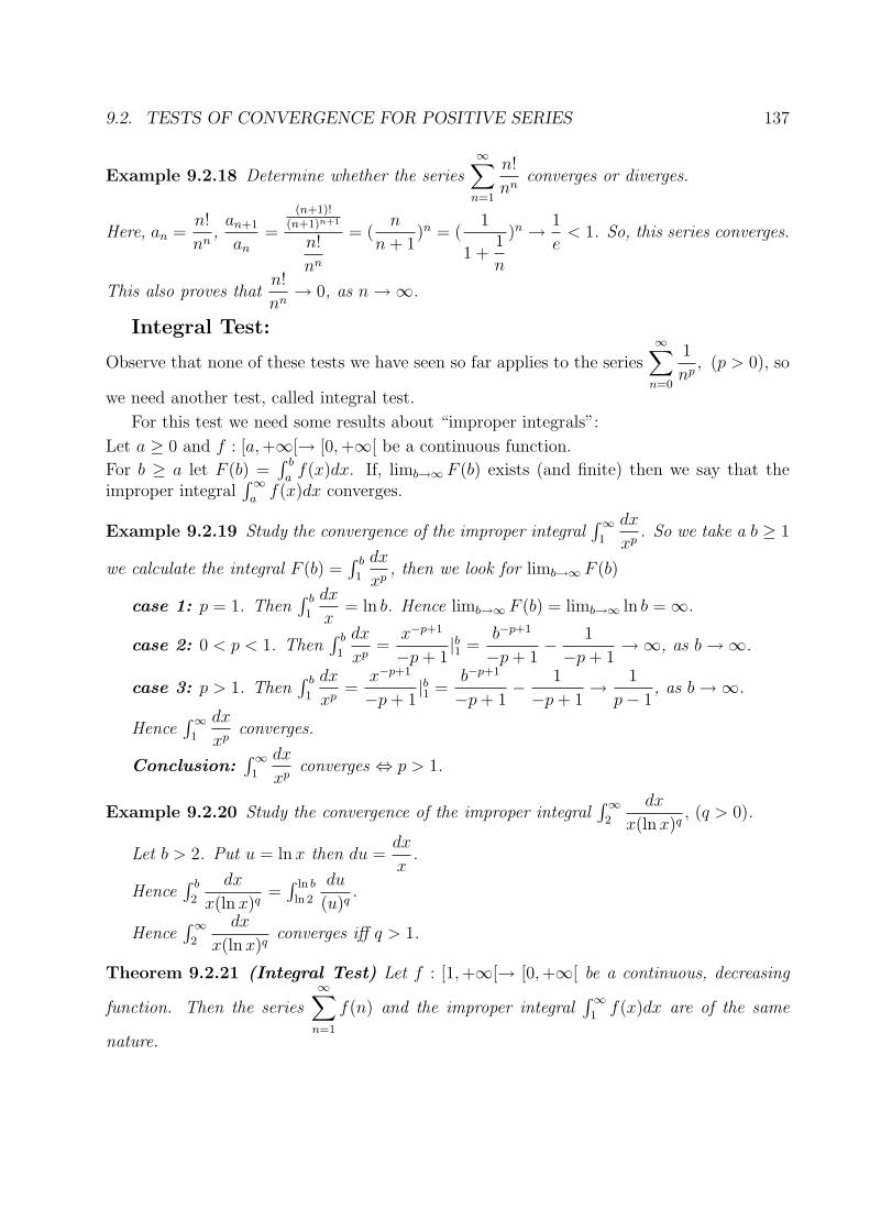
9.2. TESTS OF CONVERGENCE FOR POSITIVE SERIES 137
Example 9.2.18 Determine whether the series∞∑
n=1
n!
nnconverges or diverges.
Here, an =n!
nn,
an+1
an
=
(n+1)!(n+1)n+1
n!
nn
= (n
n + 1)n = (
1
1 +1
n
)n → 1
e< 1. So, this series converges.
This also proves thatn!
nn→ 0, as n → ∞.
Integral Test:
Observe that none of these tests we have seen so far applies to the series∞∑
n=0
1
np, (p > 0), so
we need another test, called integral test.
For this test we need some results about “improper integrals”:
Let a ≥ 0 and f : [a, +∞[→ [0, +∞[ be a continuous function.
For b ≥ a let F (b) =∫ b
af(x)dx. If, limb→∞ F (b) exists (and finite) then we say that the
improper integral∫∞
af(x)dx converges.
Example 9.2.19 Study the convergence of the improper integral∫∞1
dx
xp. So we take a b ≥ 1
we calculate the integral F (b) =∫ b
1
dx
xp, then we look for limb→∞ F (b)
case 1: p = 1. Then∫ b
1
dx
x= ln b. Hence limb→∞ F (b) = limb→∞ ln b = ∞.
case 2: 0 < p < 1. Then∫ b
1
dx
xp=
x−p+1
−p + 1|b1 =
b−p+1
−p + 1− 1
−p + 1→ ∞, as b → ∞.
case 3: p > 1. Then∫ b
1
dx
xp=
x−p+1
−p + 1|b1 =
b−p+1
−p + 1− 1
−p + 1→ 1
p − 1, as b → ∞.
Hence∫∞1
dx
xpconverges.
Conclusion:∫∞
1
dx
xpconverges ⇔ p > 1.
Example 9.2.20 Study the convergence of the improper integral∫∞
2
dx
x(ln x)q, (q > 0).
Let b > 2. Put u = ln x then du =dx
x.
Hence∫ b
2
dx
x(ln x)q=∫ ln b
ln 2
du
(u)q.
Hence∫∞2
dx
x(ln x)qconverges iff q > 1.
Theorem 9.2.21 (Integral Test) Let f : [1, +∞[→ [0, +∞[ be a continuous, decreasing
function. Then the series∞∑
n=1
f(n) and the improper integral∫∞1
f(x)dx are of the same
nature.

138 CHAPTER 9. NUMERICAL SERIES
Proof 9.2.22 Let an = f(n), ∀n ∈ N. For each n ≥ 1, and n ≤ x ≤ n + 1, since f isdecreasing, f(n + 1) ≤ f(x) ≤ f(n), i.e. an+1 ≤ f(x) ≤ an for x ∈ [n, n + 1].
Integrating this inequalities on the interval [n, n + 1] we get;∫ n+1
nf(n + 1)dx ≤ ∫ n+1
nf(x)dx ≤ ∫ n+1
nf(n)dx
i.e. an+1 ≤∫ n+1
nf(x)dx ≤ an, ∀n ≥ 1.
Hence,N∑
n=1
an+1 ≤∫ N+1
1
f(x)dx ≤N∑
n=1
an
and alsoN∑
n=1
f(n) ≤∫ N+1
1
f(x)dx + f(1) ≤ f(1) +N∑
n=1
f(n)
Put Sn = a1 + a2 + ... + an, then above inequalities becomes;
Sn+1 − a1 ≤∫ n+1
1f(x)dx ≤ Sn
SN ≤ ∫ N+1
1f(x)dx + f(1) ≤ a1 + Sn
Form this inequalities the conclusion follows.
Moreover, in the case where the convergence occurs, we have;
S − a1 ≤∫∞1
f(x)dx ≤ S where S =∞∑
n=1
an
Example 9.2.23 1. The series∞∑
n=1
1
npconverges ⇔ p > 1. Take f(x) =
1
xp,
f : [1, +∞[→ R+, and apply theorem 9.2.21.
2. The series∞∑
n=1
1
n ln ndiverges, since
∫∞2
dx
x ln xdiverges.
9.3 Absolute and Unconditional Convergence
Let∞∑
n=0
an be an arbitrary series. To such a series we cannot apply the above tests, but we
can apply them to the series∞∑
n=0
|an|.
Question: What relation is there between the convergence of the series∞∑
n=0
an and∞∑
n=0
|an|?

9.3. ABSOLUTE AND UNCONDITIONAL CONVERGENCE 139
Definition 9.3.1 A series∞∑
n=0
an is said to be absolutely convergent if the positive series
∞∑n=0
|an| converges.
As we shall see later the series∞∑
n=1
(−1)n
nconverges.
Actually∞∑
n=1
(−1)n+1
n= ln 2. But
∞∑n=1
|(−1)n
n| =
∞∑n=1
1
ndiverges. Hence, “convergence” and
“absolute convergence” are not equivalent notions.
Theorem 9.3.2 Every absolutely convergent series∞∑
n=0
an converges.
Proof 9.3.3 Let Sn = a0 + ... + an, Tn = |a0| + ... + |an|. As the series∞∑
n=0
|an| converges,
Tn is Cauchy.So, we have:
∀ε > 0, ∃N ∈ N : ∀n ≥ N, ∀p ∈ N |Tn+p − Tn| = Tn+p − Tn = |an+1| + ... + |an+p| < ε.
Hence, ∀n ≥ N ∀p ∈ N, |Sn+p − Sn| = |an+1 + ... + an+p| ≤ |an+1| + ... + |an+p| < ε.
Thus, Sn is Cauchy, so it converges. This means that the series∞∑
n=0
an converges.
Example 9.3.4 If in R, xn → x, then |xn| → |x|.
So if∞∑
n=0
an converges absolutely,
|∞∑
n=0
an| = lim |n∑
k=0
ak| ≤ limn∑
k=0
|ak| =∞∑
n=0
|an|, i.e. |∞∑
n=0
an| ≤∞∑
n=0
|an|.
Example 9.3.5 We have just seen that the series∞∑
n=1
(−1)n
nconverges, although it is not
absolutely convergent. Let us calculate the sum of the series.
We know that ln(1 + x)′ =1
1 + x=
1
1 − (−x)=
∞∑n=0
(−x)n =∞∑
n=0
(−1)nxn.
limm→∞ limn→∞(1 +1
n)m = 1, and limn→∞ limm→∞(1 +
1
n)m = ∞.
Hence, integrating we get:∫ x
0(ln(1 + x))′dx = ln(1 + x) =
∞∑n=0
(−1)n xn+1
n + 1=
∞∑n=0
(−1)n+1xn
n.

140 CHAPTER 9. NUMERICAL SERIES
Hence, ln 2 =∞∑
n=0
(−1)n+1
n= 1 − 1
2+
1
3− 1
4+ ... +
(−1)n+1
n+ ...
Now, write this sum taking one positive term then two negative terms:
(1 − 1
2− 1
4) + (
1
3− 1
6− 1
8) + ...
Now, add another parenthesis:
[(1− 1
2)− 1
4]+ [(
1
3− 1
6)− 1
8]+ ... =
1
2− 1
4+
1
6− 1
8+
1
10− 1
12+ ... =
1
2(1− 1
2+
1
3− 1
4+ ...)
Conclusion:1
2ln 2 = ln 2 !
This absurdity shows that in a series - even if it is convergent - we cannot change the orderof the terms in an infinite sum.
Question: When can we change the order of the terms without obtaining divergent seriesor different sums?
Definition 9.3.6 Let∞∑
n=0
an be a series and σ : N → N be a bijection. Then the series
∞∑n=0
aσ(n) is said to be a rearrangement of the given series.
Example 9.3.7 Let∞∑
n=0
an be a series. If σ(0) = 81, σ(1) = 92, σ(2) = 301, ..., then
∞∑n=0
aσ(n) = a81 + a92 + a301 + ...
Definition 9.3.8 A series∞∑
n=0
an is said to be unconditionally convergent if every re-
arrangement of this series converges.
Example 9.3.9 It is easy to see that the series∞∑
n=0
(−1)n
nis convergent but not uncondi-
tionally convergent.
9.3.1 Absolutely Convergent vs. Unconditionally Convergent
Theorem 9.3.10 If a series∞∑
n=0
an is absolutely convergent, then it is unconditionally con-
vergent and that for every bijection σ : N → N,∞∑
n=0
aσ(n) =∞∑
n=0
an.

9.3. ABSOLUTE AND UNCONDITIONAL CONVERGENCE 141
Proof 9.3.11 Let M =∞∑
n=0
|an| and let σ : N → N be any bijection. Then ∀n ∈ N,
n∑i=0
|aσ(i)| ≤ M . Hence the series∞∑
n=0
aσ(n) is absolutely convergent, so convergent.
Let S =∞∑i=0
ai, i.e. S = limn→∞n∑
i=0
ai
∀ε > 0, ∃N ∈ N : ∀n ≥ N |S −n∑
i=0
ai| = |∞∑
i=n+1
ai| < ε.
In particular, for all n ≥ N and m ≥ N , |m∑
i=n
ai| < ε. (∗)
Now, let N be large enough to have: {0, 1, ..., N} ⊆ {σ(0), ..., σ(N)}. Then, for n ≥ N ,
|n∑
i=0
ai −n∑
i=0
aσ(i)| = | a sum of some terms ai with i > N | < ε by (∗).
Now, sincen∑
i=0
ai → S, we see thatn∑
i=0
aσ(i) → S, too, as n → ∞.
Hence∞∑i=0
aσ(i) =∞∑i=0
ai.
We have seen that every absolutely convergent series is unconditionally convergent. We aregoing to show that converse is also true.
Let∞∑
n=0
an be a series in R. Let a+n = sup{an, 0} and a−
n = sup{−an, 0}
Then a+n ≥ 0, and a−
n ≥ 0.
Hence a+n + a−
n = |an|, and an − an = an. (∗∗)Also a+
n ≤ |an|, and a−n ≤ |an|.
Lemma 9.3.12 If∞∑
n=0
an converges but∞∑
n=0
|an| diverges then both series∞∑
n=0
a+n and
∞∑n=0
a−n
diverges to +∞.
Proof 9.3.13 Suppose for a contradiction, the series∞∑
n=0
a+n converges and
∞∑n=0
a−n diverges
to ∞.
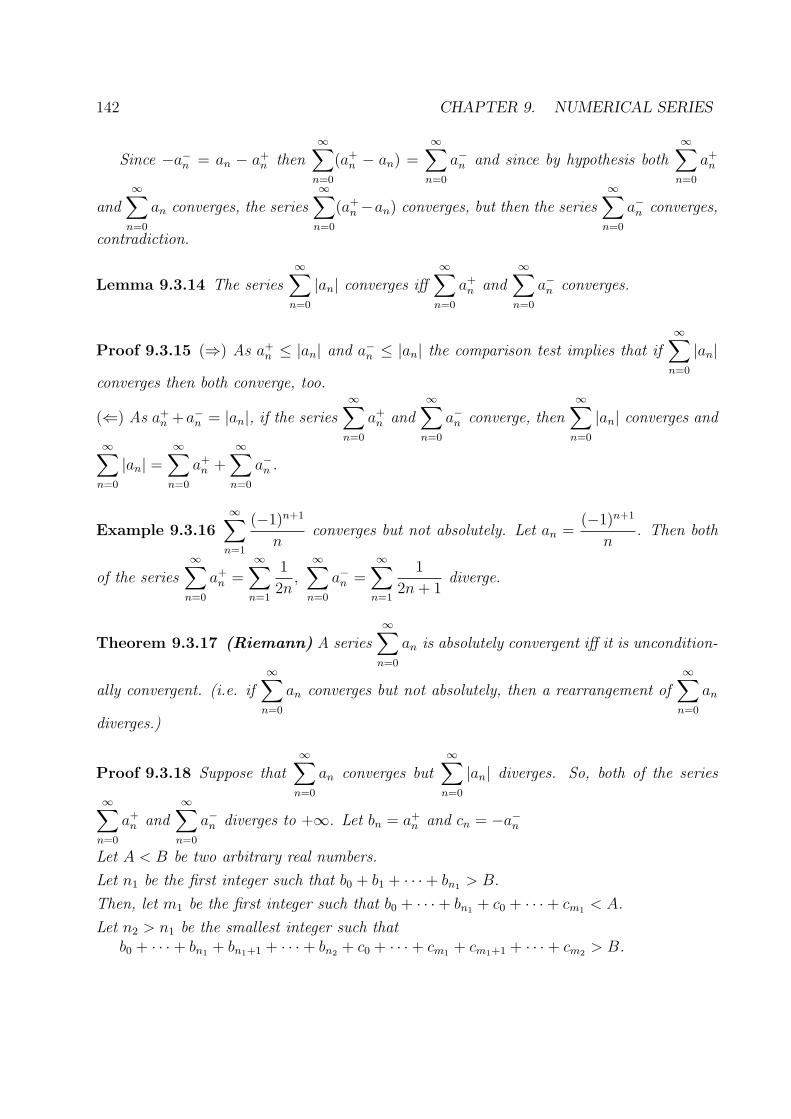
142 CHAPTER 9. NUMERICAL SERIES
Since −a−n = an − a+
n then∞∑
n=0
(a+n − an) =
∞∑n=0
a−n and since by hypothesis both
∞∑n=0
a+n
and∞∑
n=0
an converges, the series∞∑
n=0
(a+n −an) converges, but then the series
∞∑n=0
a−n converges,
contradiction.
Lemma 9.3.14 The series∞∑
n=0
|an| converges iff∞∑
n=0
a+n and
∞∑n=0
a−n converges.
Proof 9.3.15 (⇒) As a+n ≤ |an| and a−
n ≤ |an| the comparison test implies that if∞∑
n=0
|an|converges then both converge, too.
(⇐) As a+n +a−
n = |an|, if the series∞∑
n=0
a+n and
∞∑n=0
a−n converge, then
∞∑n=0
|an| converges and
∞∑n=0
|an| =∞∑
n=0
a+n +
∞∑n=0
a−n .
Example 9.3.16∞∑
n=1
(−1)n+1
nconverges but not absolutely. Let an =
(−1)n+1
n. Then both
of the series∞∑
n=0
a+n =
∞∑n=1
1
2n,
∞∑n=0
a−n =
∞∑n=1
1
2n + 1diverge.
Theorem 9.3.17 (Riemann) A series∞∑
n=0
an is absolutely convergent iff it is uncondition-
ally convergent. (i.e. if∞∑
n=0
an converges but not absolutely, then a rearrangement of∞∑
n=0
an
diverges.)
Proof 9.3.18 Suppose that∞∑
n=0
an converges but∞∑
n=0
|an| diverges. So, both of the series
∞∑n=0
a+n and
∞∑n=0
a−n diverges to +∞. Let bn = a+
n and cn = −a−n
Let A < B be two arbitrary real numbers.
Let n1 be the first integer such that b0 + b1 + · · · + bn1 > B.
Then, let m1 be the first integer such that b0 + · · · + bn1 + c0 + · · · + cm1 < A.
Let n2 > n1 be the smallest integer such thatb0 + · · · + bn1 + bn1+1 + · · · + bn2 + c0 + · · · + cm1 + cm1+1 + · · · + cm2 > B.

9.4. ABEL AND DIRICHLET TESTS 143
Then, let m2 > m1 be the smallest integer such thatb0 + · · · + bn1 + bn1+1 + · · · + bn2 + c0 + · · · + cm1 + cm1+1 + · · · + cm2 < A....
In this way we produce a rearrangement of the series∞∑
n=0
an such that, if Tn is the partial
sum of this rearrangement, Tn > B for infinitely many n and Tn < A for infinitely many n.Hence (Tn)n∈N diverges. i.e., the rearranged series, b0 + · · ·+ bn1 + c0 + · · ·+ cm1 + bn1+1 + · · ·diverges.
Definition 9.3.19 If a series∞∑i=0
ai converges but∞∑i=0
|ai| diverges, then we say that∞∑i=0
ai
is conditionally convergent.
9.4 Abel and Dirichlet Tests
None of the tests we have seen so far applies to a series to a series of the form∞∑
n=1
sin nx
n.
If we put an = sin nx, bn =1
nthen the series
∞∑n=1
sin nx
nis a series of the form
∞∑n=1
(anbn)
with bn decreasing to 0.
Or put an = (−1)n and bn =1√n
for the series∞∑
n=1
(−1)n
√n
with bn decreasing to 0.
Abel Formula - First Form: Let A0 = 0, A1 = a1, ..., An = a1 + ... + an so thatA1 − A0 = a1, A2 − A1 = a2, ..., An − An−1 = an. Then;
anb1 + ... + anbn = (A1 − A0)b1 + ... + (An − An−1)bn
= A1(b1 − b2) + A2(b2 − b3) + ... + An−1(bn−1 − bn) + Anbn.
Thus,n∑
k=1
akbk =n−1∑k=1
Ak(bk − bk+1) + Anbn.
Abel Formula - II (Cauchy Form): Let, for n ≥ m, Am,n = am + am+1 + ... + an so thatAm,m = am, Am+1,m − Am,m = am+1, ..., Am,n − Am,n−1 = an. Hence,
ambm + am+1bm+1 + ... + anbn = Am,mbm + (Am+1,m − Am,m)bm+1 + ... + (Am,n − Am,n−1)bn
= Am,m(bm − bm+1) + ... + Am,n−1(bn−1 − bn) + Am,nbn
Thus,n∑
k=m
akbk =n−1∑k=m
Am,k(bk − bk+1) + Am,nbn.
Theorem 9.4.1 (Dirichlet Test) Consider a series of the form∞∑
n=1
anbn with:

144 CHAPTER 9. NUMERICAL SERIES
1. bn ≥ 0, bn decreases to zero.
2. ∃M > 0 : ∀n ∈ N, |a1 + ... + an| ≤ M .
Then the series∞∑
n=1
anbn converges.
Proof 9.4.2 Let Sn =n∑
k=1
akbk. Then for n ≥ m,
Sn − Sm−1 =n∑
k=m
akbk =n−1∑k=m
Am,k(bk − bk+1) + Am,nbn. Then;
|Sn − Sm−1| ≤n−1∑k=m
|Am,k||bk − bk+1| + |Am,n| bn
≤n−1∑k=m
M(bk − bk+1) + Mbn
= M [(bm − bm+1) + ... + (bn−1 − bn) + bn]= Mbm → 0 as m → ∞
Hence Sn is Cauchy, so converges. Hence our series converges.
Example 9.4.3 Show that for all x ∈ R the series∞∑
n=1
sin nx
n; x �= 2kπ, converges.
Here an = sin nx, bn =1
nso bn ↓ 0. Hence, it is enough to show that ∃M > 0 such that
| sin x + ... + sin nx| ≤ M. (M may depend on x but not on n)
To calculate the sum sin x+ ...+sin nx let An = cos x+ ...+cos nx, Bn = sin x+ ...+sin nx.Then;
An + iBn = eix + e2ix + ... + einx = eix[1 + ein + ... + ei(n−1)]
= eix 1−einx
1−eix = eix ein2 x[e−
in2 x−e
in2 x]
ei2 x[e−
ix2 −e
ix2 ]
= ei n+12
x sin(n2
x)
sin x2
= (cos n+12
x + i sin(n+12
x))sin(
n
2x)
sin x2
Hence, An = cos x+...+cos nx = cos(n+12
x)sin(n
2x)
sin x2
, Bn = sin x+...+sin nx = sin(n+12
x)sin(n
2x)
sin x2
Hence, | sin x + ... + sin nx| ≤ 1
| sin x2| for x �= 2kπ, k ∈ Z
Hence by Dirichlet test, the series∞∑
n=1
sin nx
nconverges for every x �= 2kπ, (k ∈ Z). In
particular, for x ∈ [0, 2π] this series converges.

9.5. PRODUCT OF SERIES 145
Remark also that if instead of1
n, we take
1√n
,1
p√
n, ... or any bn ≥ 0, bn ↓ 0 the calculation
will be the same.
Theorem 9.4.4 (Leibniz Test) Let bn ≥ 0, bn ↓ 0. Then she alternating series∞∑
n=1
(−1)n bn
converges.
Proof 9.4.5 Let an = (−1)n So that |a1 + ...+an| ≤ 1. Hence Dirichlet test applies. So ourseries converges.
Example 9.4.6 The series∞∑
n=1
(−1)n
n,
∞∑n=1
(−1)n
√n
,
∞∑n=1
(−1)n
10√
nconverge.
Theorem 9.4.7 (Abel Test) Consider a series of the form∞∑
n=1
anbn. Suppose that:
1. The series∞∑
n=0
an is convergent.
2. (bn)n∈N is positive, monotone and bounded.
Then the series∞∑
n=1
anbn converges.
Proof 9.4.8 We can assume that (bn)n∈N is increasing and since it is bounded, bn → b, for
some b ∈ R. Then (b − bn) ↓ 0. As∞∑
n=0
an converges, Sn = a0 + ... + an converges. So,
∃M > 0 such that |Sn| ≤ M , ∀n ≥ 1. Hence by Dirichlet test the series∞∑
n=1
an(b − bn)
converges. So,∞∑
n=1
anbn = −∞∑
n=1
an(b − bn) + b
∞∑n=1
an converges.
9.5 Product of Series
Let∞∑
n=0
an and∞∑
n=0
bn be two series. If we multiply them “formally” then we get an infinite
matrix:
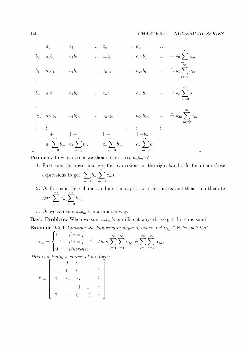
146 CHAPTER 9. NUMERICAL SERIES
⎡⎢⎢⎢⎢⎢⎢⎢⎢⎢⎢⎢⎢⎢⎢⎢⎢⎢⎢⎢⎢⎢⎢⎢⎢⎢⎢⎢⎢⎢⎢⎣
a0 a1 . . . an . . . a2n . . .
b0 a0b0 a1b0 . . . anb0 . . . a2nb0 . . .+→ b0
∞∑m=0
am
b1 a0b1 a1b1 . . . anb1 . . . a2nb1 . . .+→ b1
∞∑m=0
am
...
bn a0bn a1bn . . . anbn . . . a2nbn . . .+→ bn
∞∑m=0
am
...
b2n a0b2n a1b2n . . . anb2n . . . a2nb2n . . .+→ b2n
∞∑m=0
am
......
......
......
......
↓ + ↓ + ↓ + ↓ +bn
a0
∞∑m=0
bm a1
∞∑m=0
bm an
∞∑m=0
bm an
∞∑m=0
bm
⎤⎥⎥⎥⎥⎥⎥⎥⎥⎥⎥⎥⎥⎥⎥⎥⎥⎥⎥⎥⎥⎥⎥⎥⎥⎥⎥⎥⎥⎥⎥⎦
Problem: In which order we should sum these anbm’s?
1. First sum the rows, and get the expressions in the right-hand side then sum these
expressions to get:∞∑
n=0
bn(∞∑
m=0
am)
2. Or first sum the columns and get the expressions the matrix and them sum them to
get:∞∑
n=0
an(∞∑
m=0
bm)
3. Or we can sum anbm’s in a random way.
Basic Problem: When we sum anbm’s in different ways do we get the same sum?
Example 9.5.1 Consider the following example of sums. Let αi,j ∈ R be such that
αi,j =
⎧⎪⎨⎪⎩
1 if i = j
−1 if i = j + 1
0 otherwise
Then∞∑
j=1
∞∑i=1
αi,j �=∞∑i=1
∞∑j=1
αi,j.
This is actually a matrix of the form:
T =
⎡⎢⎢⎢⎢⎢⎢⎢⎣
1 0 0 · · · · · ·−1 1 0
...
0. . . . . . . . .
...... −1 1
...
0 · · · 0 −1...
⎤⎥⎥⎥⎥⎥⎥⎥⎦

9.5. PRODUCT OF SERIES 147
9.5.1 Cauchy Method of Sum
Now, letc0 = a0b0
c1 = a0b1 + a1b0
c2 = a0b2 + a1b1 + a2b0...cn = a0bn + a1bn−1 + · · · + anb0...
Formally, we should have:
(∞∑
n=0
an)(∞∑
n=0
bn) =∞∑
n=0
∞∑m=0
bnam =∞∑
m=0
∞∑n=0
bnam =∞∑
n=0
cn.
Theorem 9.5.2 Let∞∑
n=0
an and∞∑
n=0
bn be two absolutely convergent series and define cn =
a0bn+a1bn−1+· · ·+anb0. Then the series∞∑
n=0
cn is also absolutely convergent and (∞∑
n=0
an)(∞∑
n=0
bn) =
∞∑n=0
∞∑m=0
bnam =∞∑
m=0
∞∑n=0
bnam =∞∑
n=0
cn.
Proof 9.5.3 Let Sn = a0 + · · · + an, Tn = b0 + · · · + bn, Wn = c0 + · · · + cn
GRAFIK
SnTn = the sum of all aibj in the smaller square.Wn = the sum of all aibj in the triangle (I).W2n = the sum of all aibj in the triangle (II).
Suppose first that all ai ≥ 0, bn ≥ 0. Then Wn ≤ SnTn ≤ W2n. If Sn → S and Tn → t thenWn being bounded from above, converges. Hence Wn → T · S.
As, our series are absolutely convergent, |SnTn − Wn| ≤ SnTn − Wn → 0.
Here Sn = |a0| + · · · + |an|, Tn = |b0| + · · · + |bn|, Wn = |a0||b0| + · · · + |an||bn|
Hence Wn → T · S. i.e. (∞∑
n=0
an)(∞∑
n=0
bn) =∞∑
n=0
cn.
Example 9.5.4 Consider the series∞∑
n=0
xn
n!and
∞∑n=0
yn
n!. For every x, y ∈ R, these series
converge absolutely by ratio test.
Let us determine the product of this series.
148 CHAPTER 9. NUMERICAL SERIES
Let an =xn
n!, bn =
yn
n!and cn = a0bn + · · · + anb0. Then we know that:
(∞∑
n=0
an)(∞∑
n=0
bn) =∞∑
n=0
cn.
Now let us calculate cn :
cn = 1 · yn
n!+
x
1!· yn−1
(n − 1)!+ · · · + y
1!· xn−1
(n − 1)!+ 1 · xn
n!
=1
n!
[yn +
nx
1!yn−1 + · · · + xn
]=
1
n!(x + y)n
So that∞∑
n=0
cn =∞∑
n=0
1
n!(x + y)n.
Let S(x) =∞∑
n=0
xn
n!, S(y) =
∞∑n=0
yn
n!, then we see that:
1. S(x)S(y) = S(x + y).
2. S(0) = 1 so that S(x − x) = S(x)S(−x) = S(0) = 1, so that S(−x) =1
S(x)
Hence1
∞∑n=0
xn
n!
=∞∑
n=0
1
n!(−x)n.
3. S(x) �= 0, ∀x ∈ R, since S(x)S(−x) = 1.
In mathematics, instead of S(x) we write ex.

9.6. EXERCISES 149
9.6 Exercises
1. Show that
(a) limn→∞ n√
n = 1.
(b) For any m > 0 and any α > 0, limn→∞(ln n)m
nα= 0.
(c) For any k > 0, limn→∞ nke−1n = 0.
2. Test the following series for convergence or divergence.
(a)∞∑
n=0
nn
n!
(b)∞∑
n=0
(1 + 1n)
en
(c)∞∑
n=1
ln(1 + 1n)
(d)∞∑
n=1
1
nln(1 + 1
n)
(e)∞∑
n=1
(−1)n
n ln(1 + n)
(f)∞∑
n=1
(−1)n(1 + n)n
nn+1
3. Let an ≥ 0. Show that∞∑
n=1
an converges ⇒∞∑
n=1
√an
nconverges.
4. Let ∞∑n=0 an be a convergent series and (bn)n∈N monotone bounded sequence. Show
that the series∞∑
n=0
anbn converges.
5. Let an > 0 for all n ∈ N. Show that the series∞∑
n=0
an converges iff the series∞∑
n=0
an
1 + an
converges.
6. Let an ∈ R. Show that∞∑
n=0
|an| < ∞ →∞∑
n=0
|an|2 < ∞
150 CHAPTER 9. NUMERICAL SERIES
7. Let an ∈ R, bn ∈ R. Show that;∞∑
n=0
|an|2 < ∞ and∞∑
n=0
|bn|2 < ∞ ⇒∞∑
n=0
|anbn|2 < ∞.
8. Let x ∈ R be fixed. Show that the series∞∑
n=1
sin nx√n
converges.
9. Let a, b be 2 constants with 0 < a < b. Show that the series
1 + a + ab + a2b + a2b2 + a3b3 + a4b3 + ...
• converges if
(a) b < 1, or
(b) a < 1 < b and ab > 1.
• diverges if a < 1 < b and ab > 1.
10. Let∞∑
n=0
an, (an ∈ R) be a series. Show that;
(a) If for some p > 1, limn→∞ npan = 0, then the series∞∑
n=0
an converges absolutely.
(b) If limn→∞ nan = A and A �= 0, the series∞∑
n=0
an diverges.
(c) If limn→∞ nan = 0, we cannot conclude.

Chapter 10
Sequences and Series of Functions
1. Sequences of functions: Pointwise and Uniform Convergence
2. Uniform Convergence and Continuity, Differentiation and Integration
3. Series of Functions: Pointwise and Uniform Convergence
4. Tests for Uniform Convergence: Weierstrass M-test, Abel and DirichletTests
5. Differentiation and Integration of Series of Functions
6. Power Series and Taylor Expansion
7. Continuous but Nowhere Differentiable Functions
10.1 Sequences of Functions
Let E be any set and (Y, d′) be a m.s. Let for each n ∈ N, fn : E → (Y, d′) be a function.Then we say that we have a sequence of functions (fn)n∈N from E to Y .
Example 10.1.1 fn : [0, 1] → R fn(x) = sin nx, fn(x) = xn, fn(x) =1
1 + xn
10.1.1 Pointwise Convergence
Definition 10.1.2 Let (fn)n∈N be a sequence of functions from E to (Y, d′). If for each xin E the sequence (fn(x))n∈N converges in Y to some point yx ∈ Y , then we say that (fn)n∈N
converges pointwise on the set E.Since, in any m.s. limit is unique, for each x ∈ E, there is only one yx ∈ Y such thatfn(x) → yx. So, if we define f : E → Y by f(x) = yx we get a new function. For thisfunction we have: ∀x ∈ E, f(x) = limn→∞ fn(x), in Y . This function f is said to be thepointwise limit of the sequence (fn)n∈N on the set E.
151

152 CHAPTER 10. SEQUENCES AND SERIES OF FUNCTIONS
We write this as “fn → f pointwise on E”.
fn → f pointwise on E ⇔ ∀x ∈ E, αn(x) = |fn(x) − f(x)| → 0⇔ ∀x ∈ E, ∀ε > 0, ∃N = N(ε, x) ∈ N : ∀n ≥ N, |fn − f(x)| < ε⇔ ∀x ∈ E, ∀ε > 0, ∃N = N(ε, x) ∈ N : ∀m,n ≥ N, |fn(x) − fm(x)| < ε
Example 10.1.3 1. Let fn : [0, 1] → R, fn(x) = xn.
Then fn(0) = 0 → 0, fn(1) = 1 → 1 and For 0 < x < 1, fn(x) = xn → 0.
Let f(x) =
{0 if 0 ≤ x < 11 otherwise
Thus fn → f pointwise on [0, 1]. Observe that fn is continuous on [0, 1] but f is notcontinuous at x = 1.
Observe that although each fn is continuous on [0, 1], the limit function is not contin-uous.
2. Let fn : [0,∞[→ R, fn(x) =1
1 + xn. Then fn(0) = 1 → 1.
For 0 < x < 1, xn → 0, fn(x) → 1.
For x = 1, fn(x) =1
2→ 1
2.
For x > 1, fn(x) → 0.
Hence the pointwise limit function of the sequence (fn)n∈N on the set E = [0,∞[ is,
f(x) =
⎧⎨⎩
1 for 0 ≤ x < 112
for x = 10 for x > 1
3. Let fn : R → R, fn(x) =sin nx
n. Then ∀x ∈ R, fn(x) → 0. Hence f ≡ 0 on R is the
pointwise limit function of fn in R.
But f ′n(x) = cos nx and f ′
n(π) = (−1)n diverges.
4. Let fn : [0, 1] → R be the following:
GRAFIK
fn(x) =
⎧⎪⎪⎪⎪⎨⎪⎪⎪⎪⎩
2n2x if 0 ≤ x ≤ 1
2n
2n − 2n2x if1
2n≤ x ≤ 1
n
0 if1
n≤ x ≤ 1
Now, for x = 0, fn(0) = 0 → 0. For x > 0 for some N ∈ N, x >1
N. Hence, for
n ≥ N fn(x) = 0. Hence, for any x ∈ [0, 1], fn(x) → 0.

10.1. SEQUENCES OF FUNCTIONS 153
Now∫ 1
0fn(x)dx = Area of the triangle = 1. Hence limn→∞
∫ 1
0fn(x)dx = 1.
On the other hand∫ 1
0(limn→∞ fn(x))dx =
∫ 1
00dx = 0.
Thus, limn→∞∫ 1
0fn(x)dx �= ∫ 1
0(limn→∞ fn(x))dx.
5. Let fn : [0, 1] → R, fn(x) = xn. Then limn→∞ limx∈[0,1], x→1 fn(x) = 1.
But limx∈[0,1[, x→1 limn→∞ fn(x) = 0.
Hence, limx∈[0,1[, x→1 limn→∞ fn(x) �= limn→∞ limx∈[0,1], x→1 fn(x).
10.1.2 Uniform Convergence
Definition 10.1.4 Let fn : E → Y be a sequence of functions. We say that (fn)n∈N con-verges uniformly on E to a function f : E → Y if we have:
∀ε > 0, ∃N ∈ N, ∀n ≥ N, ∀x ∈ E, d′(fn(x), f(x)) < ε⇔ αn = supx∈E d′(fn(x), f(x)) → 0, as n → ∞⇔ ∀ε > 0, ∃N ∈ N,∀n ≥ N, supx∈E |fn(x) − f(x)| < ε
Remark: From the definition, clearly, uniform convergence implies pointwise convergence.Hence, in order to find out whether a given sequence (fn)n∈N converges uniformly on E, firstwe must determine its pointwise limit f and try to see if αn = supx∈E d′(fn(x), f(x)) goes ornot to zero.
Example 10.1.5 1. Let fn : [0, 1] → R, fn(x) = xn, we know that fn → f pointwise on[0, 1], where f is defined in example 10.1.3 and
αn = sup0≤x≤1 |fn(x) − f(x)| ≥ |fn(1 − 1
n) − f(1 − 1
n)| = (1 − 1
n)n → 1
e. So αn � 0.
So the convergence is not uniform.
2. Now let 0 < β < 1 is any fixed number and E = [0, β]. fn : E → R, fn(x) = xn. Thenfn → f ≡ 0 on E pointwise.
Moreover, αn = supx∈E |fn(x) − f(x)| = βn → 0. Hence fn → f ≡ 0 uniformly on E.
3. Let fn(x) =x
ne
xn for x ∈ [0,∞[. For each x ∈ [0,∞[, fn(x) → 0. So fn → f ≡ 0
on [0,∞[ pointwise. But βn = |fn(n) − f(n)| = e. So convergence is not uniform on[0,∞[.
4. Let fn : R → R, fn(x) =sin nx
nthen fn → f ≡ 0 pointwise on R. Also
supx∈R |fn(x) − f(x)| = supx∈R
∣∣∣∣sin nx
n
∣∣∣∣ ≤ 1
n→ 0.
5. Let fn, f : E → Y be some functions. If supx∈E d′(fn(x), f(x)) ≤ βn and βn → 0, thenfn → f uniformly on E.
154 CHAPTER 10. SEQUENCES AND SERIES OF FUNCTIONS
Cauchy Condition for Uniform Convergence:
Definition 10.1.6 Let fn : E → Y be a sequence of functions. We say that (fn)n∈N isuniformly Cauchy on E if we have:
∀ε > 0, ∃N ∈ N, ∀n,m ≥ N, ∀x ∈ E, d′(fn(x), f(x)) < ε or supx∈E d′(fn(x), f(x)) < ε.
Theorem 10.1.7 Suppose that (Y, d′) is complete. fn : E → Y a sequence of functionsconverges uniformly on E iff it is uniformly Cauchy on E.
Proof 10.1.8 (⇒) Suppose that fn converges uniformly on E. So we have:
∀ε > 0, ∃N ∈ N, ∀n ≥ N supx∈E d′(fn(x), f(x)) < ε.
Then ∀n,m ≥ N, supx∈E d′(fn(x), f(x)) < 2ε.
(⇐) Conversely suppose fn is uniformly Cauchy, so we have:
∀ε > 0, ∃N ∈ N, ∀n,m ≥ N supx∈E d′(fn(x), fm(x)) < ε (1)
Hence, for each x ∈ E, (fn(x))n∈N is Cauchy in Y . As (Y, d′) is complete, (fn)n∈N convergesto some point yn ∈ Y .
Let f(x) = yx. Then fn → f pointwise on E. Let us see that the convergence is uniform.
Let x ∈ E be any point. Since fn → f , we have:
∀ε > 0, ∃Mx ∈ N : ∀m ≥ Mx, d′(fm(x), f(x)) < ε.
Now, let N be as in (1) (So N does not depend on x !)
Let n ≥ N, then for m ≥ max{N, Mx},d′(fn(x), f(x)) ≤ d′(fn(x), fm(x)) + d′(fm(x), f(x)) < 2ε
So we have,
∀ε > 0, ∃N ∈ N (which does not depend on x), ∀n ≥ N ∀x ∈ E d′(fn(x), f(x)) < 2ε.
So, fn → f uniformly on E.
Remark : Let E be any set and B(E) = {f : E → R, f is bounded}. On B(E) we put the“supremum metric”, i.e. d(f, g) = supx∈E |f(x) − g(x)|.Now, let fn, f ∈ B(E). It is clear that fn → f uniformly on E ⇔ d(fn, f) → 0.
Theorem 10.1.9 Let (X, d), (Y, d′) be two m.s., A ⊆ X a set, a ∈ A a point and fn : A → Ybe arbitrary functions. Suppose that (Y, d′) is complete and
1. (fn)n∈N converges uniformly on A to some f : A → Y .
2. ∀n ∈ N, limx∈A, x→a fn(x) = Ln exists.
Then limn→∞ limx∈A, x→a fn(x) = limx∈A, x→a limn→∞ fn(x).

10.2. CONTINUITY, DIFFERENTIATION AND INTEGRATION 155
Proof 10.1.10 Since f(x) = limn→∞ fn(x) and Ln = limx∈A, x→a fn(x) it is enough to showthat (Ln)n∈N converges and limn→∞ Ln = limx∈A, x→a f(x). Let us write what we have:
(fn)n∈N is uniformly Cauchy: ∀ε > 0, ∃N ∈ N : ∀n,m ≥ N, ∀x ∈ A, d′(fn(x), f(x)) < ε (∗)Since N is independent of x in A, fixing n ≥ N and m ≥ N arbitrarily and letting x → a(x ∈ A), we get : d′(Ln, Lm) ≤ ε. (because in any m.s d is a continuous function, i.e.xn → x, yn → y =⇒ d(xn, yn) → d(x, y))
Hence Ln is Cauchy in (Y, d′), so converges to a certain L ∈ Y .
In (∗) fix an m ≥ N and x ∈ A arbitrary and let m → ∞. Then we get:
∀ε > 0 ∃N ∈ N : ∀n ≥ N, ∀x ∈ A, d′(fn(x), f(x)) < ε.
In this last expression letting x → a, x ∈ A we get:
∀ε > 0, ∃N ∈ N : ∀n ≥ N, limx→a d′(fn(x), f(x)) ≤ ε.
As, limx∈A, x→a fn(x) = Ln we conclude that limn→∞ Ln = limx∈A, x→a f(x).
Example 10.1.11 fn : [0, 1[→ R, fn(x) = xn
Then, limn→∞ limx<1, x→1 fn(x) �= limx<1, x→1 limn→∞ fn(x). Hence, fn � f ≡ 0 uniformlyon [0, 1[.
10.2 Continuity, Differentiation and Integration
10.2.1 Uniform Convergence and Continuity
Theorem 10.2.1 Let fn : A → Y be a sequence of functions and a ∈ A. Suppose that(Y, d′) is complete and
1. each fn is continuous at a.
2. (fn)n∈N converges uniformly on A to some function f : A → Y .
Then f is continuous at a.
Proof 10.2.2 By the theorem 10.1.9,limx∈A, x→a f(x) = limx∈A, x→a[limn→∞ fn(x)]
= limn→∞ limx∈A, x→a fn(x)= limn→∞ fn(a) = f(a)
Hence f is continuous at a.
Remark: By contrapositive, if each fn is continuous on A, fn → f pointwise on A and f isnot continuous at some point a ∈ A then the convergence is not uniform on A. For instance,
if fn = xn on [0, 1], then fn → f =
{1 if x = 1
0 if x �= 1
As f is not continuous at a = 1, we conclude that the convergence is not uniform on [0, 1].

156 CHAPTER 10. SEQUENCES AND SERIES OF FUNCTIONS
10.2.2 Metric Nature of Uniform Convergence
Let E be any set and B(E){f : E → R : f is bounded }. For f, g ∈ B(E), letd∞(f, g) = supx∈E |f(x) − g(x)|. This is a metric on B(E).
For fn, f ∈ B(E), d∞(fn, f) → 0 ⇔ fn → f uniformly on E.
For that reason d∞ is called the metric of uniform convergence.
We have already seen that (B(E), d∞) is complete.
Now, let Cb(E) = {f : E → R : f is continuous and bounded on E}. On Cb(E) put thesupremum metric, d∞. Obviously, Cb(E) ⊆ B(E)
Theorem 10.2.3 (Cb(E), d) is complete.
Proof 10.2.4 1. Cb(E) ⊆ B(E).
2. (B(E), d) is complete.
3. Cb(E) is closed in B(E) by the theorem 10.2.1, indeed let (fn)n∈N be a sequence inCb(E) that converges (for the supremum metric) to some f ∈ (B)(E). But then by thetheorem 10.2.1 f is continuous on E, so f ∈ Cb(E).
4. In any complete m.s (X, d), a subspace (M, d) is complete iff M is closed in X.
Particular Case: Let K ⊆ X be a compact set and C(K) = {f : K → R : f is continuous on K},then obviously each f ∈ C(K) is bounded on K. Then (C(K), d) is a complete m.s. In par-ticular the space C([0, 1]) is a complete m.s under the supremum metric. (i.e. uniformconvergence metric)
Example 10.2.5 C0(R) = {f : R → R : lim|x|→∞ f(x) = 0, f is continuous} is complete.
Example 10.2.6 Let fn : [0,∞[→ R, fn(x) =1
1 + xn.
Then fn(x) → f(x) =
⎧⎪⎨⎪⎩
1, if 0 ≤ x < 112, if x = 1
0, if x > 1
As f is not continuous on [0,∞[ and each fn is continuous on the same set, we concludethat convergence of fn to f is not uniform on [0,∞[.
10.2.3 Uniform Convergence and Integration
Theorem 10.2.7 Let fn : [a, b] → R be a sequence of continuous functions. Suppose that(fn)n∈N converges uniformly to some f : [a, b] → R on [a, b]. Then,
1. Fn(x) =∫ x
afn(t)dt → F (x) =
∫ x
af(t)dt uniformly on [a, b].

10.2. CONTINUITY, DIFFERENTIATION AND INTEGRATION 157
2.∫ b
a|fn(t) − f(t)|dt → 0, as n → ∞.
3. limn→∞∫ b
afn(x)dx =
∫ b
a(limn→∞ fn(x))dx.
Proof 10.2.8 Since fn → f uniformly on [a, b], we have:∀ε > 0, ∃N ∈ N : ∀n ≥ N, ∀x ∈ [a, b], |fn(x) − f(x)| < ε.
Hence, for n ≥ N and ∀x ∈ [a, b],
| ∫ x
afn(t)dt − ∫ x
af(t)dt| ≤ ∫ b
a|fn(t) − f(t)|dt ≤ ∫ x
a(ε)dt ≤ ∫ b
a(ε)dt ≤ ε(b − a).
So, Fn → F uniformly on [a, b]. And 2 and 3 follows from this.
Example 10.2.9 Let fn : [0, 1] → R, fn(x) =
⎧⎪⎨⎪⎩
2n2x if 0 ≤ x ≤ 1/2n
2n − 2n2x if 1/2n ≤ x ≤ 1/n
0 if 1/n ≤ x ≤ 1
Then, as we have seen, fn → f ≡ 0 pointwise on [0, 1].∫ 1
0fn(x)dx =
1
2, ∀n ∈ N, limn→∞
∫ 1
0fn(x)dx =
1
2�= ∫ 1
0f(x)dx.
Hence, the convergence is not uniform on [0, 1].
Example 10.2.10 limn→∞∫ a
0cos nxdx =
sin nx
n
∣∣∣∣a0
=sin na
n→ 0. But (cos nx)n∈N con-
verges iff x = 2kπ, k ∈ Z.
10.2.4 Uniform Convergence and Differentiation
Theorem 10.2.11 Let fn : [a, b] → Rbe a sequence of continuously differentiable functions.(i.e. f ′
n(x) exists and continuous on [a, b] ∀n ∈ N) Suppose that:
1. (f ′n(x))n∈N converges uniformly on [a, b] to some function g : [a, b] → R.
2. For some x0 ∈ [a, b], the numerical sequence (f ′n(x0))n∈N converges to some L ∈ R.
Then (fn)n∈N converges uniformly to some f : [a, b] → R. This f is differentiable and f ′ = gon [a, b].
Proof 10.2.12 By ”Newton - Leibniz Theorem” fn(x) = fn(x0) +∫ x
x0f ′
n(t)dt. Then, by
theorem 10.2.7, fn(x) → f(x) = L +∫ x
x0g(t)dt uniformly on [a, b]. Hence, f ′(x) = g(x) on
[a, b].
Example 10.2.13 Let fn(x) =sin nx
non [a, b]. Then fn → f ≡ 0 uniformly on [a, b].
(fn)n∈N is continuously differentiable and f ′n(x) = cos nx. But (f ′
n)n∈N does not convergeeven pointwise.
158 CHAPTER 10. SEQUENCES AND SERIES OF FUNCTIONS
10.3 Series of Functions
Definition 10.3.1 Let E be a set and fn : E → R be a sequence of functions. The formal
sum∞∑
n=0
fn(x) is said to be a “series of functions” on the set E.
10.3.1 Pointwise Convergence of Function Series
Definition 10.3.2 If, for each x ∈ E, the “numerical series”∞∑
n=0
fn(x) converges, then we
say that the function series converges pointwise on E.
In this case, we obtain a function f : E → R, by putting f(x) = limn→∞ Sn(x), whereSn = f0 + f1 + · · · + fn. By definition, f is the “pointwise sum of the series”. We write this
as f(x) =∞∑
n=0
fn(x) pointwise on E.
For instance, for every x ∈ R, the series∞∑
n=1
xn
n!converges. So it defines a function f(x) =
∞∑n=1
xn
n!. We know that f(x) = ex.
Remark Let fn be any sequence of functions on a set E. To this sequence associate the
function series f0 +∞∑
n=0
(fn+1 − fn). Let Sn = f0 +n−1∑k=0
(fk+1 − fk) = fn be the partial sum
of this series. Consequently, the series f0 +∞∑
n=0
(fn+1 − fn) converges pointwise on E iff fn
converges pointwise on E.
From this we conclude that:
1. If E is a subset of some m.s. (X, d) and each term gn of the series∞∑
n=0
gn(x) is continuous
on E and g(x) =∞∑
n=0
gn(x) (pointwise on E), the function g need not to be continuous
on E. e.g. let fn(x) = xn, 0 ≤ x ≤ 1 and g0 = f0, gn = fn+1 − fn. Then g is thepointwise limit of fn on [0, 1], which is not continuous.
2. Similarly if each gn : [a, b] → R continuous and we have g(x) =∞∑
n=0
gn(x) pointwise on
[a, b], in general we don’t have:∫ b
a
( ∞∑n=0
gn(x)
)dx =
∞∑n=0
(∫ b
a
gn(x)dx
).

10.3. SERIES OF FUNCTIONS 159
3. If each gn : [a, b] → R is continuously differentiable on [a, b] and g(x) =∞∑
n=0
gn(x)
pointwise on [a, b], in general we do not have:
( ∞∑n=0
gn(x)
)′
=∞∑
n=0
g′n(x).
10.3.2 Uniform Convergence of the Function Series
Let E be any set and∞∑
n=0
fn(x) be a series of functions on E. Let Sn = f0 + f1 + · · ·+ fn be
the partial sum of this series. So we have a “sequence” of functions, Sn.
Definition 10.3.3 If this Sn converges uniformly on E to a function f , then we say that∞∑
n=0
fn(x) converges uniformly to f on E. We write this as, f =∞∑
n=0
fn(x) uniformly
on E. This is equivalent to say that Sn is uniformly Cauchy, i.e.
∀ε > 0, ∃N ∈ N : ∀n ≥ N, ∀p ∈ N, supx∈E
∣∣∣∣∣n+p∑k=n
fk(x)
∣∣∣∣∣ < ε.
Remark: From this definition we conclude that a “necessary” (not sufficient) condition for
the uniform convergence of the series∞∑
n=0
fn(x) on E, is the uniform convergence of fn to
zero on E.
For instance, the series∞∑
n=0
xn converges pointwise on [0, 1[ but not uniformly since xn → 0
pointwise but not uniformly.
Example 10.3.4 Let∞∑
n=0
fn(x) be a series and Sn = f0 + f1 + · · · + fn be its partial sum.
If for some sequence xn ∈ E, (Sm(xn))n∈N does not converge, then fn(xn) � 0 and so thisseries cannot converge uniformly.
Example 10.3.5 Consider the series∞∑
n=0
xn
n!. For every x ∈ R, this series converges to ex.
Is this convergence uniform on R ?
A necessary condition for uniform convergence is the uniform convergence of fn(x) =xn
n!to
zero on R, i.e. supx∈R
∣∣∣∣xn
n!
∣∣∣∣→ 0.
But supx∈R
∣∣∣∣xn
n!
∣∣∣∣ ≥ nn
n!→ ∞. So convergence of this series to ex is not uniform on R.

160 CHAPTER 10. SEQUENCES AND SERIES OF FUNCTIONS
However, on every compact interval [a, b] convergence is uniform. To see this, we use the
Cauchy condition: supa≤x≤b
∣∣∣∣∣n+p∑k=n
xk
k!
∣∣∣∣∣ ≤n+p∑k=n
|b|kk!
→ 0, as n → ∞, if |b| ≥ a.
Example 10.3.6 Consider the series∞∑
n=0
xn.
Here Fn(x) = 1 + x + · · · + xn =
⎧⎨⎩
1 − xn+1
1 − xfor x �= 1
n + 1, for x = 1
• For |x| ≥ 1 the series diverges since xn � 0.
• For |x| < 1, xn → 0, so Fn(x) → f(x) =1
1 − xpointwise on ] − 1, 1[ so that
∞∑n=0
xn =1
1 − xpointwise on ] − 1, 1[.
• The convergence is not uniformly on ] − 1, 1[ since for instance, for x = 1 − 1
n + 1,
Fn
(1 − 1
n + 1
)=
−(1 − 1n+1
+ 1)
1 − 1 + 1n+1
→ e−1.
Thus limx→1 limn→∞ Fn(x) = e−1 but limn→∞ limx→1 Fn(x) does not exist (actually ∞)
• Now let 0 < α < 1, then∞∑
n=0
xn converges uniformly on ] − α, α[ to1
1 − x. Indeed,
sup|x|≤α
∣∣∣∣Fn(x) − 1
1 − x
∣∣∣∣ = sup|x|≤α
∣∣∣∣ xn+1
1 − x
∣∣∣∣ ≤ αn+1
1 + α→ 0
Hence∞∑
n=0
xn converges pointwise on ] − 1, 1[ to1
1 − x, and the convergence is uniform on
[−α, α] for any 0 < α < 1.
10.3.3 Hereditary Properties
Theorem 10.3.7 (Continuity) Let A be a subset of a m.s. (X, d). fn : A → R sequenceof functions and x0 ∈ A. If;
• The series∞∑
n=0
fn converges uniformly on A and
• Each fn is continuous at x0
Then the function f =∞∑
n=0
fn is continuous at x0.
(i.e. limx∈A, x→x0
∞∑n=0
fn(x) =∞∑
n=0
limx∈A, x→x0
fn(x))

10.4. TESTS FOR UNIFORM CONVERGENCE 161
Proof 10.3.8 Let Fn = f0 + f1 + · · ·+ fn, then (Fn)n∈N converges uniformly on A and each
Fn is continuous at x0. Then by theorem 10.2.1, limn→∞ Fn = limn→∞n∑
i=0
fi =∞∑
n=0
fn = f
is continuous at x0.
Theorem 10.3.9 (Integration) Let fn : [a, b] → R be a sequence of functions. Suppose
that the series∞∑
n=0
fn converges uniformly on [a, b]. Then∫ a
x(
∞∑n=0
fn(t))dt =∞∑
n=0
∫ a
x
fn(t)dt
Proof 10.3.10 Let Fn = f0 + f1 + · · ·+ fn, then (Fn)n∈N converges uniformly on [a, b] to F .
Then by theorem 10.2.7, limn→∞∫ a
xFn(t)dt =
∞∑n=0
∫ x
a
fn(t)dt =
∫ x
a
F (t)dt =
∫ x
a
(∞∑
n=0
fn(t))dt
Theorem 10.3.11 (Differentiation) Let fn : [a, b] → R be continuously differentiable on[a, b]. Suppose that;
• the series∞∑
n=0
f ′n converges uniformly on [a, b]
• for x0 ∈ [a, b], the numerical series∞∑
n=0
fn(x0) converges.
Then the series∞∑
n=0
fn converges uniformly to f =∞∑
n=0
fn and
f ′ =
( ∞∑n=0
fn
)′
=∞∑
n=0
f ′n
Proof 10.3.12 Let Fn = f0 + f1 + · · · + fn, then each F ′n is continuous on [a, b] and F ′
n
converges uniformly on [a, b], also for x0 ∈ [a, b], (Fn(x0))n∈N converges in R. Then by
theorem 10.2.11, Fn converges uniformly on [a, b] to F = limn→∞ Fn =∞∑
n=0
fn and F is
differentiable on [a, b] and that F ′ =∞∑
n=0
f ′n
10.4 Tests for Uniform Convergence
Let∞∑
n=0
fn (x) be an arbitrary series of functions on a set E.
Theorem 10.4.1 (Weierstrass M-Test): Suppose that supx∈E |fn(x)| ≤ αn and that the
numerical series∞∑
n=0
αn is convergent. Then the series∞∑
n=0
fn(x) converges uniformly on E.

162 CHAPTER 10. SEQUENCES AND SERIES OF FUNCTIONS
Proof 10.4.2 Let Sn = f0 + f1 + · · · + fn. Let us see that Sn is uniformly Cauchy on E.
As∞∑
n=0
αn is convergent its partial sum An = α0 + α1 + · · · + αn is a Cauchy sequence. We
have: ∀ε > 0, ∃N ∈ N : ∀n ≥ N, ∀p ∈ N, |An+p − An| = αn+1 + · · · + αn+p < ε. Then∀n ≥ N, ∀p ∈ N,
supx∈E |Sn+p(x) − Sn(x)| = supx∈E |fn+1(x) + · · · + fn+p(x)|≤ supx∈E |fn+1(x)| + · · · + supx∈E |fn+p(x)|≤ αn+1 + · · · + αn+p < ε
.
So, Sn is uniformly Cauchy on E. Hence the series∞∑
n=0
fn(x) converges uniformly.
Example 10.4.3 Consider the series∞∑
n=0
xn
n. Determine the largest set E ⊆ R on which
this series converges uniformly.
This series converges pointwise on [−1, 1[, diverges at any point x /∈ [−1, 1[. The conver-gence is uniform on any compact interval [a, b] ⊆] − 1, 1[.
Remark: Let A be a subset of some m.s. (X, d). Let S : A → R be a continuous andbounded function. Then supx∈A |S(x)| = supx∈A |S(x)|. Hence, if each fn : A → R is
continuous, then if the convergence of the series∞∑
n=0
fn(x) is not uniform on A. So it cannot
be uniform on A.
� Weierstrass-M test cannot be applied e.g. to the series∞∑
n=1
sin nx
n. So we need another
test.
10.4.1 Abel and Dirichlet Tests for Uniform Convergence
Consider a series of the form∞∑
n=0
fn(x)gn(x), where fn, gn : E → R are arbitrary functions
defined on a set E. To study the convergence of this series, we need the “Cauchy form” ofthe Abel formula.
Consider the numerical series of the form∞∑
n=1
anbn.
Put A0 = 0, A1 = a1, . . . , An = a1 + · · · + an.
Let m > n be integers, Sn =n∑
k=1
akbk and Sm − Sn−1 =m∑
k=n
akbk = anbn + · · · + ambm.
Then an = An − An−1, an+1 = An+1 − An, . . . , am = Am − Am−1
So that;

10.4. TESTS FOR UNIFORM CONVERGENCE 163
Sm − Sn = bn(An − An−1) + bn+1(An+1 − An) + · · · + bm(Am − Am−1)= −bnAn−1 + An(bn − bn+1) + · · · + Am−1(bm−1 − bm) + bmAm
Theorem 10.4.4 (Dirichlet Test) Let E be a set, fn, gn : E → R be arbitrary functions.Suppose that;
1. gn ≥ 0 is decreasing and gn → 0 uniformly on E.
2. ∃M > 0, supx∈I
∣∣∣∣∣n∑
i=0
fi(x)
∣∣∣∣∣ < M, ∀n ∈ N.
Then the series∞∑
n=1
fn(x)gn(x) converges uniformly on E.
Proof 10.4.5 Let Sn(x) =n∑
k=1
fk(x)gk(x), we want to show that (Sn(x))n∈N is uniformly
Cauchy on E.
Since gn → 0 uniformly on E, ∀ε > 0, ∃N ∈ N, ∀n ≥ N, supx∈E gn(x) < ε.
Now put An = f1 + · · · + fn, with A0 = 0. Then,
Sn+p − Sn−1 = fngn + fn+1gn+1 + · · · + fn+pgn+p =
p∑k=0
An+k(gn+k − gn+k−1) + An+pgn+p.
As, |An+p(x)gn+p(x)| ≤ M |gn+p(x)|,
supx∈I
∣∣∣∣∣p∑
k=0
An+k(gn+k(x) − gn(x))
∣∣∣∣∣ ≤ M supx∈I |gn+p(x) − gn(x)| ≤ Mε, ∀x ∈ E.
Hence, Sn is uniformly Cauchy on I. So it converges uniformly on I.
Example 10.4.6 Study the uniform convergence of the series∞∑
n=1
sin nx
n.
Here, gn(x) =1
n↓ 0, and fn(x) = sin nx. We know that |sin x + · · · + sin nx| ≤ 1∣∣sin x
2
∣∣ on
any compact interval [a, b] ⊆]0, 2π[, supa≤x≤b
1∣∣sin x2
∣∣ < ∞.
Hence, this series converges uniformly on any compact interval [a, b] ⊆]0, 2π[.
Theorem 10.4.7 (Abel Test) Let fn, gn be two sequences of bounded functions and;
1.∞∑
n=0
fn(x) converges uniformly on E to a bounded function f : E → R.
2. gn is monotone on E and converges uniformly on E to some function g : E → R.

164 CHAPTER 10. SEQUENCES AND SERIES OF FUNCTIONS
Then the series∞∑
n=0
fn(x)gn(x) converges uniformly on E.
Proof 10.4.8 Let g = limn→∞ gn. Then (g − gn) decreases uniformly to 0 on E.
As,∞∑
n=0
fn(x) converges uniformly on E to a bounded function f : E → R, ∃M > 0 such
that supx∈E
∣∣∣∣∣n∑
i=0
fi(x)
∣∣∣∣∣ ≤ M , ∀n ≥ 1.
Hence, by the Dirichlet Test (theorem 10.4.4),∞∑
n=0
fn(x)(g(x) − gn(x)) converges uniformly.
So,∞∑
n=0
fn(x)gn(x) =∞∑
n=0
fn(x)(g(x) − gn(x)) + g(x)∞∑
n=0
fn(x) converges uniformly.
10.5 Power Series and Taylor Expansion
Let an ∈ R and x0 ∈ R be given. A series of the form∞∑
n=0
an(x− x0)n is said to be a power
series about x0.
Lemma 10.5.1 Consider a power series∞∑
n=0
anxn. Let z ∈ R be a number. Then,
1. If∞∑
n=0
anzn converges, then for any |x| < |z|, the series
∞∑n=0
anxn converges.
2. If∞∑
n=0
anzn diverges, then for any |x| > |z|, the series
∞∑n=0
anxn diverges.
Proof 10.5.2 1. Suppose∞∑
n=0
anzn converges. Then lim sup n
√(anzn) ≤ 1. Then for
|x| < |z| lim sup n√
(anxn) = |x| lim sup n√|m| < |z| lim sup n
√|m| ≤ 1.
Hence, lim sup n√
(anxn) < 1. Hence,∞∑
n=0
anxn converges absolutely, so converges.
2. Suppose that∞∑
n=0
anzn diverges. Then lim sup n√
(anzn) ≥ 1.
Hence for |x| > |z|, lim sup n√
(anxn) = |x| lim sup n√|m| > |z| lim sup n
√|m| ≥ 1 =⇒lim sup n
√(anxn) > 1.

10.5. POWER SERIES AND TAYLOR EXPANSION 165
Hence,∞∑
n=0
anxn diverges.
Conclusion: Given any power series∞∑
n=0
an(x−x0)n, there exists a symmetric interval about
x0 of the form ]R − x0, R + x0[ such that:
1. ∀x ∈ ]R − x0, R + x0[, the series∞∑
n=0
an(x − x0)n converges absolutely.
2. ∀x /∈ [R − x0, R + x0], the series∞∑
n=0
an(x − x0)n diverges.
Hence, the domain of convergence of any power series is an interval.
Example 10.5.3 Consider the function series∞∑
n=1
cos nx
n.
• For x = π,∞∑
n=1
cos nπ
n=
∞∑n=1
(−1)n
nconverges.
• For x = −π it also converges.
• But −π < 0 < π,∞∑
n=1
cos n0
n=
∞∑n=1
1
ndiverges. So the domain of this series is not an
interval.
Example 10.5.4 Consider the power series∞∑
n=0
n!xn. This series converges for x = 0 only.
So the “interval of convergence” for power series might be degenerated, [0, 0] = {0}.
Example 10.5.5 Consider the power series∞∑
n=1
(−1)n
nxn. This series converges for x = 1
but diverges for x = −1. It also converges for any |x| < 1. Hence its interval of convergenceis ] − 1, 1] .
10.5.1 Radius of Convergence of a Power Series
Let∞∑
n=0
anxn be a power series. Let ρ = lim sup n√|an|. (we take ρ = ∞ if the sequence
n√|an| is not bounded)
Let R =1
ρ. (we put R = 0, if ρ = ∞ and R = ∞, if ρ = 0)

166 CHAPTER 10. SEQUENCES AND SERIES OF FUNCTIONS
This R is said to be the “radius of convergence” of the power series∞∑
n=0
anxn.
R =1
lim sup n√|an|
.
Theorem 10.5.6 Let∞∑
n=0
an(x− x0)n be a power series and R be its radius of convergence.
Then,
1. ∀x ∈ R, |x − x0| < R, this series converges absolutely.
2. ∀x ∈ R, |x − x0| > R, this series diverges.
3. ∀x ∈ R, |x − x0| = R, we cannot conclude.
4. ∀r ∈ R, 0 ≤ r ≤ R on the compact interval [r − x0, r + x0], the convergence is uniform.
Proof 10.5.7 1. Let x ∈ R be such that |x − x0| < R. Then lim sup n√|an(x − x0)n| =
|x − x0| lim sup n√|an| =
|x − x0|R
< 1.
Hence the series∞∑
n=0
an(x − x0)n converges absolutely.
2. Let x ∈ R be such that |x − x0| > R. Then lim sup n√|an(x − x0)n| > 1.
Hence, the series∞∑
n=0
an(x − x0)n diverges.
3. See below examples.
4. Let 0 ≤ r ≤ R. Let |x − x0| ≤ r. Then sup|x−x0|≤r |an(x − x0)n| ≤ |an| rn. Now,
the positive series∞∑
n=0
|an| rn converges since lim sup n√|an| rn =
r
R< 1. Hence by
“Weierstrass-M test” the series∞∑
n=0
an(x−x0)n converges uniformly on [r − x0, r + x0].
Example 10.5.8 1. Consider the series∞∑
n=0
xn
n. Here R =
1
lim n√
n= 1. Hence;
for x ∈] − 1, 1[ this series converges,
for x = 1 this series diverges,
for x = −1 this series converges,
for 0 < r < 1 this series converges uniformly on [−r, r].

10.5. POWER SERIES AND TAYLOR EXPANSION 167
2. Consider the series∞∑
n=0
xn
n!. Here an =
1
n!.
As,an+1
an
→ 0, lim n√
an → 0.
Hence, R = ∞. i.e., ∀x ∈ R, the series∞∑
n=0
xn
n!converges. But convergence is not
uniform on R. Since supx>0
∣∣∣∣∣n∑
k=1
xk
k!
∣∣∣∣∣ > supx>0
xn
n!≥ nn
n!↓ 0.
Theorem 10.5.6(4) says that for any compact interval [−a, a], the convergence is uniform.Hence, in theorem 10.5.6(3) we cannot take r = R.
10.5.2 Differentiation and Integration of Power Series
Now, let∞∑
n=0
an(x−x0)n be a power series and ]R−x0, R+x0[ be its interval of convergence.
Let x be any point in this interval so that |x − x0| < R. Let |x − x0| < r < R, so thatx ∈ [r − x0, r + x0].
Now, for each x ∈]R−x0, R+x0[, let f(x) =∞∑
n=0
an (x − x0)n be the sum of this series. Since
each term of the series is a continuous function and convergence is uniform on the interval[r − x0, r + x0], f is continuous at x. Thus, f is continuous on ]R − x0, R + x0[.
Recall: If an ≥ 0, bn ≥ 0 and an → L, then lim sup(anbn) = lim an lim sup bn
Lemma 10.5.9 Let∞∑
n=0
an(x−x0)n be a power series. Then the radius of convergence of the
series∞∑
n=0
nan(x−x0)n−1 and
∞∑n=0
an
n + 1(x−x0)
n+1 are the same as the radius of convergence
of the series∞∑
n=0
an(x − x0)n.
Proof 10.5.10 Let R be the radius of convergence of the series∞∑
n=0
an(x − x0)n. Then,
R = lim sup n√|an|.
Note that limn→∞ |n| 1n−1 = 1 and limn→∞
∣∣∣∣ 1
n + 1
∣∣∣∣1
n+1
= 1
• lim sup n−1√|nan| = lim sup
[|n| 1
n−1 |an|1
n−1
]= lim |n| 1
n−1 lim sup |an|n
n−11n
= lim sup[
n√|an|
] nn−1
= R

168 CHAPTER 10. SEQUENCES AND SERIES OF FUNCTIONS
• lim sup n+1
√ |an|n + 1
= lim n+1
√1
n + 1lim sup n+1
√|an| = lim sup[
n√|an|
] nn+1
= R.
Theorem 10.5.11 Let∞∑
n=0
an(x−x0)n be a power series and R be its radius of convergence
and for x ∈ ]R − x0, R + x0[, f(x) =∞∑
n=0
an(x − x0)n be the sum of this series.
Then on the interval ]R − x0, R + x0[, f is infinitely differentiable and
f ′(x) =∞∑
n=0
nan(x − x0)n−1, . . . , f (k)(x) =
∞∑n=0
n(n − 1) . . . (n − (k + 1))an(x − x0)n−k.
Proof 10.5.12 Since the series∞∑
n=0
an(x − x0)n has the same radius of convergence as the
initial series and that every x ∈ [r − x0, r + x0] belongs to a compact interval [a, b] ⊆]R − x0, R + x0[ and that the series
∞∑n=0
nan(x − x0)n−1 converges uniformly on [a, b], by
theorem 10.3.11 the function f is differentiable at x and f ′(x) =∞∑
n=0
nan(x − x0)n−1. The
rest is just an iteration of this.
Hence, if f(x) =∞∑
n=0
an(x−x0)n for x ∈]R−x0, R+x0[, then an =
f (n)(x0)
n!from f (n)(x0) =
n!an.
So, f(x) =∞∑
n=0
f (n)(x0)
n!(x − x0)
n. Then, if f is given as a power series, this series is just
the Taylor series of f at x0. Also, for any compact interval [a, b] ⊆]R − x0, R + x0[, f is
integrable on [a, b] and∫ b
af(x)dx =
∫ b
a
( ∞∑n=0
an(x − x0)n
)dx =
∞∑n=0
an
∫ b
a
(x − x0)ndx.
Lemma 10.5.13 Let∞∑
n=0
anxn and∞∑
n=0
bnxn be two power series. Suppose that for some
α > 0, these series converge on ] − α, α[ and∞∑
n=0
anxn =∞∑
n=0
bnxn, for each x ∈] − α, α[.
Then for each n ∈ N, an = bn.
Proof 10.5.14 Let f(x) = sum∞n=0anx
n =∞∑
n=0
bnxn, ∀x ∈] − α, α[.
Then an = bn =f (n)(0)
n!, ∀n.

10.5. POWER SERIES AND TAYLOR EXPANSION 169
Conclusion:
1. If a function f :]−α, α[→ R can be represented as the sum of a power series∞∑
n=0
anxn,
then this is the only power series whose sum is f on ] − α, α[.
2. If there is a function f :] − α, α[→ R and by any method we represent f as
f(x) =∞∑
n=0
anxn then this power series is necessarily the “Taylor series” of f on ]−α, α[.
Example 10.5.15 Let f(x) = ln(1 + x), −1 < x < 1, then f ′(x) =1
1 + x.
For −1 < x < 1,1
1 + x=
∞∑n=0
(−x)n.
Now let 0 < α < 1 and x ∈ [−α, α], then
ln(1 + x) =∫ x
0
dt
1 + t=∫ x
0
( ∞∑n=0
(−t)n
)dt =
∞∑n=0
∫ x
0
(−t)ndt =∞∑
n=0
(−1)n xn+1
n + 1.
Hence ln(1+x) =∞∑
n=0
(−1)n xn+1
n + 1and this is the Taylor series of f(x) = ln(1+x) on ]−1, 1[.
10.5.3 Analytic Functions
Now let f(x) =∞∑
n=0
anxn with radius of convergence ρ > 0, on ] − ρ, ρ[. We have seen that
such an f is infinitely differentiable on ] − ρ, ρ[.
Question: Is an infinitely differentiable function f : A → R, analytic on A?
Definition 10.5.16 Let A ⊆ R be an open set and f : A → R be a function. Let x0 ∈ A. Wesay that f is real analytic at x0 if there is R = R(x0) > 0 such that ]R− x0, R + x0[⊆ A,
and on ]R − x0, R + x0[, f is representable as a power series. (i.e. f(x) =∞∑
n=0
an(x − x0)n,
for some an ∈ R.)If f is analytic at every x0 ∈ A, then we say that f is analytic on A.
Example 10.5.17 Let f : R → R, f(x) =
{e−
1x2 , if x �= 0
0, if x = 0This f is called as the
“Cauchy function”.
Let us see that at every x ∈ R, f is infinitely differentiable and that f (n)(x0) = 0, ∀n ∈ N.
• For x �= 0, the functions ϕ(x) = − 1
x2and ψ(x) = ex are infinitely differentiable. So the
composition ψ ◦ ϕ(x) = e−1
x2 is infinitely differentiable on R \ {0}.

170 CHAPTER 10. SEQUENCES AND SERIES OF FUNCTIONS
• For x0 = 0, limx�=0, x→0f(x) − f(0)
x − 0= limx�=0, x→0
e−1
x2
x= limx �=0, x→0
1
xe1
x2
= 0.
Hence,
{f ′(0) = 0
f ′(x) =2
x3e−
1x2
limx�=0, x→0f ′(x) − f ′(0)
x= limx�=0, x→0
2x3 e
− 1x2
x= limx�=0, x→0
2
x4e1
x2
= 0.
Remark: If P (x) is any polynomial then limx �=0, x→0 P (x)e1
x2 = ∞. Hence form this wededuce that f (n)(0) = 0, ∀n ∈ N. If this f were analytic at x0 = 0, we would have R > 0
such that ∀x ∈] − R,R[, f(x) =∞∑
n=0
anxn.
Since, then an =f (n)(0)
n!on ] − R, R[, f would be identically zero, which is not the case,
since f(x) �= 0 for x �= 0. Then f is infinitely differentiable but not analytic. In “complexanalysis” every differentiable function is analytic. In real analysis this is not the case.
10.5.4 Continuity at the Boundary of Interval of Convergence
Consider a power series∞∑
n=0
anxn. Let ] − ρ, ρ[ be its interval of convergence and for x ∈
] − ρ, ρ[, f(x) =∞∑
n=0
anxn. We know that f is continuous on ] − ρ, ρ[.
Question: What can we say about the continuity of f at −ρ or ρ?
Example 10.5.18 For |x| < 1, the geometric series∞∑
n=0
xn converges and f(x) =1
1 + x=
∞∑n=0
xn on ] − 1, 1[.
Now limx→−1,x>−1 f(x) =1
2.
But∞∑
n=0
limx→−1, x>−1
xn =∞∑
n=0
(−1)n does not exist.
So that limx→−1, x>−1(∞∑
n=0
xn) exists but it is not∞∑
n=0
( limx→−1, x>−1
xn).
Theorem 10.5.19 (Abel’s Theorem) Let∞∑
n=0
anxn be a power series and 1 be its radius
of convergence and f :] − 1, 1[→ R, f(x) =∞∑
n=0
anxn.

10.5. POWER SERIES AND TAYLOR EXPANSION 171
1. If the numerical series∞∑
n=0
an converges then the series∞∑
n=0
anxn converges uniformly
on [0, 1], so that f is continuous at x = 1 and
limx→1, x<1 f(x) = limx→1, x<1
( ∞∑n=0
anxn
)=
∞∑n=0
limx→1, x<1
anxn =∞∑
n=0
an.
2. If the numerical series∞∑
n=0
(−1)nan converges then the series∞∑
n=0
anxn converges uni-
formly on [−1, 0] and f is continuous at x = −1 and∞∑
n=0
limx→−1, x>−1
anxn =
∞∑n=0
an(−1)n = limx→−1, x>−1
f(x).
Proof 10.5.20 1. Let Sn(x) =n∑
k=0
akxk and suppose that
∞∑n=0
an converges. We want to
prove that (Sn)n∈N is uniformly Cauchy on [0, 1].
Let Tn = a0 + a1 + · · · + an, as Tn is convergent by hypothesis, Tn is Cauchy so;∀ε > 0,∃N ∈ N, ∀N, ∀p ∈ N, |an + an+1 + · · · + an+p| < ε
Fix n ≥ N . Let Ap = an + an+1 + · · · + an+p, then
Sn+p(x) − Sn−1(x) = anxn + an+1xn+1 + · · · + an+px
n+p
= A0xn + (A1 − A0)x
n+1 + . . . + (Ap − Ap−1)xn+p
= A0(xn − xn+1) + A1(x
n+1 − xn+2) + · · · + Ap−1(xn+p−1 − xn+p) + Apx
n+p
= A0xn(1 − x) + A1x
n+1(1 − x) + · · · + Ap−1xn+p−1(1 − x) + Apx
n+p
As by Cauchy condition for Tn |Ai| < ε for 0 ≤ i ≤ p; for 0 ≤ x ≤ 1,
|Sn+p(x) − Sn−1(x)| ≤ (1 − x)xn[ε + εx + . . . + εxp−1] + εxn+p
= ε(1 − x)xn 1 − xp
1 − x+ εxn+p
= ε[xn − xn+p + xn+p] = εxn
So for n ≥ N, ∀p ∈ N, sup0≤x≤1 |Sn+p(x) − Sn−1(x)| ≤ sup0≤x≤1 εxn ≤ ε.
Hence Sn is uniformly Cauchy on [0, 1].
Hence f is continuous at x = 1 and limx→1, x<1 f(x) =∞∑
n=0
an
2. Use similar steps to prove.
Example 10.5.21 ln(1 + x) =∞∑
n=0
(−1)n xn+1
n + 1=
∞∑n=1
(−1)n+1xn
nfor −1 < x < 1.
We have seen that∞∑
n=0
(−1)n
nconverges.

172 CHAPTER 10. SEQUENCES AND SERIES OF FUNCTIONS
Hence by above theorem∞∑
n=0
(−1)n
n= lim
x→1, x<1ln(1 + x) = ln(2).
10.6 Continuous but Nowhere Differentiable Functions
Start with the function f(x) = |x|, for −1 ≤ x ≤ 1. Then extend this function periodicallywith period 2.
-2 -1-3
1
1 2 3 4 5 6
Figure 10.1: Graph of the function
Let g be this function. g(x) =
{|x| for − 1 ≤ x ≤ 1
g(x + 2) = g(x) ∀x ∈ R
In particular |g(x)| ≤ 1. For any x, y ∈ R, |g(x) − g(y)| ≤ ||x| − |y|| ≤ |x − y|. Let
δn =±1
2 · 4n. Observe that for any x ∈ R there is no integer in between ]x, x ± δn[. This
implies that the points x and x±δ are on the same line that composes the graph of g. Hence|g(x + δn) − g(x)| ≤ δn |g′(c)| ≤ δn for some x < c < x + δn.
Now, let f(x) =∞∑
k=0
(3
4
)k
g(4kx). By Weierstrass-M test, f is continuous on R. Let us see
that f has no tangent.
Theorem 10.6.1 This f is nowhere differentiable on R.
Proof 10.6.2 Fix a point x ∈ R. Let us prove that|f(x + δn) − f(x)|
δn
→ ∞. Since δn → 0,
as n → ∞, this proves that f is not differentiable at x0.
We have,|f(x + δn) − f(x)|
δn
=
∞∑k=0
(3
4
)k
g(4k(x + δn)) − g(4kx)
δn
For k > n, g(4k(x+ δn))−g(4kx) = g
(4kx +
4k
2 · 4n
)−g(4kx) = 0, since g is periodical with
period 2.

10.6. CONTINUOUS BUT NOWHERE DIFFERENTIABLE FUNCTIONS 173
For k = n,∣∣g(4k(x + δn)) − g(4kx)
∣∣ = ∣∣∣∣g(
4kx +1
2
)− g(4kx)
∣∣∣∣ ≤ 1
2
Next, we use the following:
|a1 + · · · + an| ≥ |a1| − |a2 + · · · + an| ≥ |a1| −n∑
k=2
|ak|.
Hence,f(x + δn) − f(x)
δn
=
(34
)ng(4n(x + δn)) − g(4nx)
δn
+n−1∑k=1
(34
)kg(4k(x + δn)) − g(4kx)
δn
.
So,
∣∣∣∣f(x + δn) − f(x)
δn
∣∣∣∣ ≥ 3n −n−1∑k=1
(34
)k ∣∣g(4k(x + δn)) − g(4kx)∣∣
δn
≥ 3n −n∑
k=1
(3
4
)k4k |δn||δn|
= 3n −n−1∑k=1
3k = 3n − 3n − 1
2=
3n + 1
2→ ∞
Hence, f is not differentiable at x.
Theorem 10.6.3 (Weierstrass Approximation Theorem) Every continuous functionon a compact interval f : [0, 1] → R is a uniform limit of a sequence of polynomial functionsPn(x) on [0, 1].
Proof 10.6.4 Observe that 1 = 1n = (x + (1 − x))n =n∑
k=0
(nk
)xk(1 − x)n−k. Hence,
f(x) =n∑
k=0
f(x)
(nk
)xk(1 − x)n−k.
Because of this let Pn(x) =n∑
k=0
f
(k
n
)(nk
)xk(1 − x)n−k. Hence, Pn is a polynomial of
degree n. These polynomials are “Bernstein polynomials associated to f”.
Let us see that sup0≤x≤1 |f(x) − Pn(x)| → 0, as n → ∞.
As f is continuous on [0, 1] and [0, 1] is compact, f is uniformly continuous. So, we have:∀ε > 0 ∃δ > 0 : ∀x, y ∈ [0, 1], (|x − y| < δ =⇒ |f(x) − f(y)| < ε).
Hence, if
∣∣∣∣x − k
n
∣∣∣∣ ≤ δ, then∣∣f(x) − f
(kn
)∣∣ < ε.
For this reason, f(x)−Pn(x) =n∑
k=0
(f(x) − f
(k
n
))ϕn(x), where ϕn(x) =
(nk
)xk (1 − x)n−k.
Then, f(x) − Pn(x) =∑
|x− kn |<δ
(f(x) − f
(k
n
))ϕk(x) +
∑|x− k
n |≥δ
(f(x) − f
(k
n
))ϕk(x),
where the sums are over k.

174 CHAPTER 10. SEQUENCES AND SERIES OF FUNCTIONS
Then for M = sup0≤x≤1 |f(x)|,
|f(x) − Pn(x)| ≤∑
|x− kn |<δ
(f(x) − f
(k
n
))ϕn(x) +
∑|x− k
n |≥δ
(f(x) − f
(k
n
))ϕn(x)
≤ ε
n∑k=0
ϕk(x) +∑
|x− kn |≥δ
(f(x) − f
(k
n
))ϕk(x)
≤ ε + 2M∑
|x− kn |≥δ
ϕk(x)
Let us see that∑
|x− kn |≥δ
ϕk(x) → 0, as n → ∞.
∣∣∣∣x − k
n
∣∣∣∣ ≥ δ =⇒(
x − k
n
)2
≥ δ2 =⇒ 1
δ2
(x − k
n
)2
≥ 1.
Hence,∑
|x− kn |≥δ
ϕk(x) ≤ 1
δ2
n∑k=0
(x − k
n
)2
ϕk(x).
Now,n∑
k=0
(x − k
n
)2
ϕk(x) =n∑
k=0
(x2 − 2x
k
n+
(k
n
)2)
ϕk(x)
= x2 − 2x
n
n∑k=0
kϕk(x) +1
n2
n∑k=0
k2ϕk(x)
To estimate last quantities, form (x + y)n =n∑
k=0
(nk
)xkyn−k, differentiate with respect to
x, and multiply by x to get;
nx(x + y)n−1 =n∑
k=0
k
(nk
)xkyn−k.
Then differentiating twice and multiplying by x2 we get:
x2n(n − 1)(x + y)n−2 =n∑
k=0
k(k − 1)
(nk
)xkyn−k.
Then replace y by 1 − x to get nx =n∑
k=0
kϕk(x) and n(n − 1)x2 =n∑
k=0
k(k − 1)ϕk(x). Then
x2 − 2x
n
n∑k=0
kϕk(x) +1
n2
n∑k=0
k2ϕk(x) = x2 − 2x2 +1
n2[n(n − 1)x2 + nx]
=x − x2
n≤ 1
n→ 0
Hence, sup0≤x≤1 |f(x) − Pn(x)| → 0, as n → ∞.
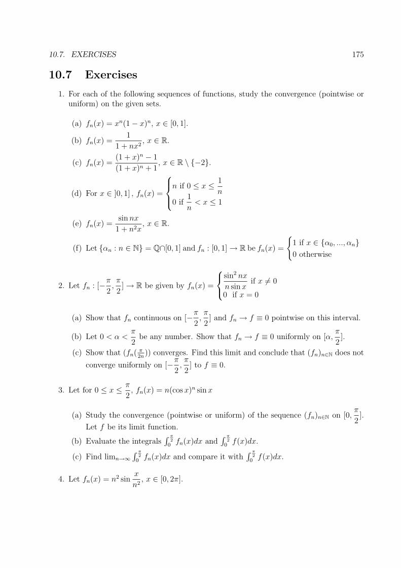
10.7. EXERCISES 175
10.7 Exercises
1. For each of the following sequences of functions, study the convergence (pointwise oruniform) on the given sets.
(a) fn(x) = xn(1 − x)n, x ∈ [0, 1].
(b) fn(x) =1
1 + nx2, x ∈ R.
(c) fn(x) =(1 + x)n − 1
(1 + x)n + 1, x ∈ R \ {−2}.
(d) For x ∈ ]0, 1] , fn(x) =
⎧⎪⎨⎪⎩
n if 0 ≤ x ≤ 1
n
0 if1
n< x ≤ 1
(e) fn(x) =sin nx
1 + n2x, x ∈ R.
(f) Let {αn : n ∈ N} = Q∩[0, 1] and fn : [0, 1] → R be fn(x) =
{1 if x ∈ {α0, ..., αn}0 otherwise
2. Let fn : [−π
2,π
2] → R be given by fn(x) =
⎧⎨⎩
sin2 nx
n sin xif x �= 0
0 if x = 0
(a) Show that fn continuous on [−π
2,π
2] and fn → f ≡ 0 pointwise on this interval.
(b) Let 0 < α <π
2be any number. Show that fn → f ≡ 0 uniformly on [α,
π
2].
(c) Show that (fn( π2n
)) converges. Find this limit and conclude that (fn)n∈N does not
converge uniformly on [−π
2,π
2] to f ≡ 0.
3. Let for 0 ≤ x ≤ π
2, fn(x) = n(cos x)n sin x
(a) Study the convergence (pointwise or uniform) of the sequence (fn)n∈N on [0,π
2].
Let f be its limit function.
(b) Evaluate the integrals∫ π
2
0fn(x)dx and
∫ π2
0f(x)dx.
(c) Find limn→∞∫ π
2
0fn(x)dx and compare it with
∫ π2
0f(x)dx.
4. Let fn(x) = n2 sinx
n2, x ∈ [0, 2π].
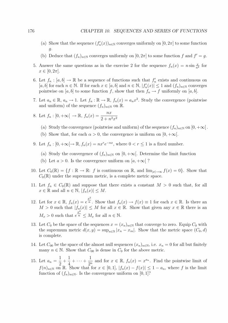
176 CHAPTER 10. SEQUENCES AND SERIES OF FUNCTIONS
(a) Show that the sequence (f ′n(x))n∈N converges uniformly on [0, 2π] to some function
g.
(b) Deduce that (fn)n∈N converges uniformly on [0, 2π] to some function f and f ′ = g.
5. Answer the same questions as in the exercise 2 for the sequence fn(x) = n sin xn2 for
x ∈ [0, 2π].
6. Let fn : [a, b] → R be a sequence of functions such that f ′n exists and continuous on
[a, b] for each n ∈ N. If for each x ∈ [a, b] and n ∈ N, |f ′n(x)| ≤ 1 and (fn)n∈N converges
pointwise on [a, b] to some function f , show that then fn → f uniformly on [a, b].
7. Let an ∈ R, an → 1. Let fn : R → R, fn(x) = anx2. Study the convergence (pointwiseand uniform) of the sequence (fn)n∈N on R.
8. Let fn : [0, +∞[ → R, fn(x) =nx
2 + n2x2
(a) Study the convergence (pointwise and uniform) of the sequence (fn)n∈N on [0, +∞[ .
(b) Show that, for each α > 0, the convergence is uniform on [0, +∞[.
9. Let fn : [0, +∞[→ R, fn(x) = nxre−nx, where 0 < r ≤ 1 is a fixed number.
(a) Study the convergence of (fn)n∈N on [0, +∞[. Determine the limit function
(b) Let a > 0. Is the convergence uniform on [a, +∞[ ?
10. Let C0(R) = {f : R → R: f is continuous on R, and lim|x|→∞ f(x) = 0}. Show thatC0(R) under the supremum metric, is a complete metric space.
11. Let fn ∈ C0(R) and suppose that there exists a constant M > 0 such that, for allx ∈ R and all n ∈ N, |fn(x)| ≤ M .
12. Let for x ∈ R, fn(x) = ex2
n . Show that fn(x) → f(x) ≡ 1 for each x ∈ R. Is there anM > 0 such that |fn(x)| ≤ M for all x ∈ R. Show that given any x ∈ R there is an
Mx > 0 such that ex2
n ≤ Mx for all n ∈ N.
13. Let C0 be the space of the sequences x = (xn)n∈N that converge to zero. Equip C0 withthe supremum metric d(x, y) = supn∈N |xn − xm|. Show that the metric space (C0, d)is complete.
14. Let C00 be the space of the almost null sequences (xn)n∈N, i.e. xn = 0 for all but finitelymany n ∈ N. Show that C00 is dense in C0 for the above metric.
15. Let an =1
2+
1
4+ · · · +
1
2nand for x ∈ R, fn(x) = xan . Find the pointwise limit of
f(n)n∈N on R. Show that for x ∈ [0, 1], |fn(x) − f(x)| ≤ 1 − an, where f is the limitfunction of (fn)n∈N. Is the convergence uniform on [0, 1]?

10.7. EXERCISES 177
16. For x ∈ [0, +∞[, let fn(x) = nxe−nx
(a) Show that (fn)n∈N converges pointwise on [0, +∞[ to some function f .
(b) Show that the convergence is not uniform on [0, +∞[ but for any α > 0, it isuniform on [α, +∞[.
17. Let b > 0. Compute∫ b
0fn(x)dx. Is limn→∞
∫ b
0fn(x)dx =
∫ b
0f(x)dx?
Is limb→∞ limn→∞∫ b
0fn(x)dx = limn→∞ limb→∞
∫ b
0fn(x)dx?
18. Let fn : [0, +∞[→ R, fn(x) =xe−
xn
n.
(a) Find the pointwise limit of f of the sequence (fn)n∈N on [0, +∞[.
(b) Show that the convergence fn → f is not uniform on [0, +∞[ but it is on [0, b] forany b > 0.
(c) Compare the iterated limits limn→∞ limb→∞∫ b
0fn(x)dx and limb→∞ limn→∞
∫ b
0fn(x)dx.
19. Let fn : R → R, fn(x) =e−n2x2
n
(a) Show that (fn)n∈N converges uniformly on R be some function f : R → R
(b) Show that f ′n → f ′ pointwise on R, but the convergence is not uniform on any
interval [−a, a] (a > 0).
178 CHAPTER 10. SEQUENCES AND SERIES OF FUNCTIONS

Chapter 11
Riemann Integral
1. Definition and Existence
2. Properties of the Riemann Integration
3. Fundamental Theorem of Calculus
4. Improper Integrals
11.1 Definition and Existence
Let f : [a, b] → R be a bounded function and m = infa≤x≤b f(x), M = supa≤x≤b f(x).
Definition 11.1.1 A partition P of [a, b] is a finite set of points in [a, b] such that, ifP = {x0, x1, · · · xn}, then a = x0 < x1 < · · · xn = b. By P ([a, b]) we denote the set of all thepossible partitions of [a, b]. The set P ([a, b]) is ordered by inclusion: P1 ≤ P2 ⇐⇒ P1 ⊆ P2.In this case P2 is said to be a “refinement” of P1.
In any partition P = {x0, x1, · · · xn} of [a, b] for i = 1, 2, . . . , n put mi = infxi−1≤x≤xif(x)
and Mi = supxi−1≤x≤xif(x)
To any partition P = {x0, x1, · · · xn} of [a, b] we associate three sums:
L(f, P ) =n∑
i=1
mi(xi − xi−1)
U(f, P ) =n∑
i=1
Mi(xi − xi−1)
R(f, P ) =n∑
i=1
f(ξi)(xi − xi−1), where ξi ∈ [xi−1, xi] is any point. (“Riemann Sum”)
It is clear that m(b − a) ≤ L(f, P ) ≤ R(f, P ) ≤ U(f, P ) ≤ M(b − a).
179

180 CHAPTER 11. RIEMANN INTEGRAL
Definition 11.1.2 A function f : [a, b] → R is said to be Riemann integrable on [a, b],if supP∈P([a,b]) L(f, P ) = infP∈P([a,b]) U(f, P ).
If this is the case and I = supP∈P([a,b]) L(f, P ) = infP∈P([a,b]) U(f, P ). Then we say that, I is
the Riemann integral of f on [a, b] and we denote this I by∫ b
af(x)dx.
If the function is Riemann integrable on [a, b],∫ b
af(x)dx = supP∈P([a,b]) L(f, P ) = infP∈P([a,b]) U(f, P ).
� R[a, b] is the set of all R-integrable functions on [a, b].
Example 11.1.3 Let f : [0, 1] → R, f(x) =
{1 if x ∈ Q0 if x ∈ R \ Q
(“Dirichlet function”).
Let P = {x0, x1, · · · , xn} be any partition of [0, 1]. Then for each i ∈ {1, . . . , n}, we havemi = infxi−1≤x≤xi
f(x) = 0Mi = supxi−1≤x≤xi
f(x) = 1
Hence, L(f, P ) = 0, U(f, P ) = 1. So, supP∈P([a,b]) L(f, P ) = 0 �= 1 = infP∈P([a,b]) U(f, P ).Hence f is not Riemann integrable on [0, 1].
Example 11.1.4 Let f : [a, b] → R, f(x) = c. Then for any P ∈ P([a, b]),L(f, P ) = c(a − b), U(f, P ) = c(a − b).
So f is R-integrable and∫ b
af(x)dx = c(b − a).
Example 11.1.5 Let y1, . . . , yn be finitely many arbitrary points in [0, 1] and f : [0, 1] → R
be the function defined by f(x) =
{ci if x = yi
0 otherwise.where ci ∈ R+ are given numbers.
Let P = {x0, x1, · · · xn} be any partition of [0, 1]. Then form the sums L(f, P ) and U(f, P ).Then L(f, P ) = 0 and U(f, P ) �= 0 but infp∈P([a,b]) U(f, P ) = 0.
Lemma 11.1.6 Let R([a, b]) = {f : [a, b] → R : f is R-integrable}. Let f : [a, b] → R be abounded function and P, P ′ be two arbitrary partitions of [a, b]. Then,
1. If P ⊆ P ′, then L(f, P ) ≤ L(f, P ′), U(f, P ) ≥ U(f, P ′)
2. L(f, P ) ≤ U(f, P ′), ∀P, P ′ ∈ P([a, b]).
Proof 11.1.7 1. Suppose P ⊆ P ′. First suppose that P ′ = P ∪ {x∗}.Then, let ki = infxi−1≤x≤x∗ f(x), ki = infxi−1≤x≤xi
f(x). Then
L(f, P ′) = m1(x1 − x0) + · · · + mi−1(xi−1 − xi−2) + mi(xi − xi−1)ki(x∗ − xi−1)
+ki(xi − x∗) + mi+1(xi+1 − xi) + · · · + mn(xn − xn−1)≥ L(f, P )
Similarly, U(f, P ′) ≤ U(f, P ).
Now, if P ′ \ P = {x∗1, . . . , x
∗k} then applying the above reasoning to P ∪ {x∗
1}, then toP ∪ {x∗
1} ∪ {x∗2}, . . ., we get L(f, P ′) ≥ L(f, P ) and U(f, P ′) ≤ U(f, P ).

11.1. DEFINITION AND EXISTENCE 181
2. Let P = P ∪ P ′. Then P ∈ P([a, b]) so that P ⊇ P and P ⊇ P ′. By 1 above,
L(f, P ) ≤ L(f, P ) ≤ U(f, P ) ≤ U(f, P ′).
Conclusion: Let A = {L(f, P ) : P ∈ P([a, b])}, A = {L(f, P ) : P ∈ P([a, b])}. Then,A,B are two bounded subsets of R. Moreover, ∀x ∈ A, ∀y ∈ B, x ≤ y.
Theorem 11.1.8 Let f : [a, b] → R be a bounded function. Then f is Riemann integrableon [a, b] ⇔ ∀ε > 0, there is a partition P ∈ P([a, b]) such that U(f, P ) − L(f, P ) < ε.
Proof 11.1.9 (⇒) Suppose f is Riemann integrable on [a, b]. Then,
I = supP∈P([a,b]) L(f, P ) = infP∈P([a,b]) U(f, P ), where I =∫ b
af(x)dx.
Hence, ∀ε > 0, ∃P1 ∈ P([a, b]) : L(f, P1) > I − ε
2, ∃P2 ∈ P([a, b]) : U(f, P2) < I +
ε
2.
Let P = P1 ∪ P2, then L(f, P ) > I − ε
2, U(f, P ) < I +
ε
2.
Hence U(f, P ) − L(f, P ) < ε.
(⇐) Conversely suppose that given any ε > 0 there is a P ∈ P([a, b]) such thatU(f, P ) − L(f, P ) < ε.
This implies that sup A = inf B. Hence f is R-integrable.
Theorem 11.1.10 Let f : [a, b] → R be a bounded function. Then f ∈ R([a, b]) iff there is anumber I ∈ R such that ∀ε > 0, ∃P0 ∈ P([a, b]) : ∀P ∈ P([a, b]), P ⊇ P0 ⇒ |R(f, P ) − I| < ε,for any choices of ξi’s in the definition of R(f, P ).
Proof 11.1.11 (⇒) Suppose first that f ∈ R([a, b]) on [a, b]. Let I =∫ b
af(x)dx and ε > 0
be arbitrary. Then as above, ∃P0 ∈ P([a, b]), L(f, P ) > I − ε
2, U(f, P ) < I +
ε
2. Hence, for
any P ⊇ P0, L(f, P ) > I − ε
2, U(f, P ) < I +
ε
2.
Then since for any choices of ξi’s, L(f, P ) ≤ R(f, P ) ≤ U(f, P ), we conclude that
−ε
2< R(f, P ) − I <
ε
2, i.e. |R(f, P ) − I| <
ε
2.
(⇐) Conversely, assume that: ∃I ∈ R, ∀ε > 0, ∃P0 ∈ P([a, b]) : ∀P ∈ P([a, b]),P ⊇ P0 ⇒ |R(f, P ) − I| < ε, for any choices of ξi’s in the definition of R(f, P ).
Take such a P ⊇ P0, so that |R(f, P ) − I| < ε, for every choices of ξi’s in the definition ofR(f, P ).
As R(f, P ) =n∑
i=1
f(ξi)(xi − xi−1), where ξi ∈ [xi−1, xi], choose ξi’s such that
f(ξi) − mi <ε
b − a. Then |L(f, P ) − R(f, P )| < ε. So, |L(f, P ) − I| < 2ε.
If we choose ξi’s such that Mi − f(ξi) <ε
b − a, then |U(f, P ) − I| < 2ε.
Hence, U(f, P ) − L(f, P ) < 4ε. So by theorem 11.1.8 f is R-integrable on [a, b].

182 CHAPTER 11. RIEMANN INTEGRAL
Lemma 11.1.12 Let f : [α, β] → R be a bounded function. Then,supα≤x≤β f(x) − infα≤x≤β f(x) = sup{f(x) − f(y) : α ≤ x, y ≤ β}
= sup{|f(x) − f(y)| : α ≤ x, y ≤ β}Theorem 11.1.13 1. If f ∈ R[a, b], then |f | ∈ R[a, b].
2. If f, g ∈ R[a, b], then f + g ∈ R[a, b].
3. If f ∈ R([a, b]) and c ∈ R is a constant, then cf ∈ R([a, b]).
Proof 11.1.14 1. Suppose f ∈ R[a, b]. Then, ∀ε > 0, ∃P0 ∈ P([a, b]) : U(f, P ) −L(f, P ) < ε. (i.e.
n∑i=1
(Mi − mi)(xi − xi−1) < ε)
Hence, Mi − mi = supxi−1≤x≤xif(x) − infxi−1≤x≤xi
f(x)
Mi − mi = sup{f(x) − f(y) : x, y ∈ [xi−1, xi]}≥ sup{|f(x)| − |f(y)| : x, y ∈ [xi−1, xi]}= supxi−1≤x≤xi
|f(x)| − infxi−1≤x≤xi|f(x)|
.
Hence, U(|f |, P ) − L(|f |, P ) ≤ U(f, P ) − L(f, P ) < ε.
Hence by theorem 11.1.8, |f | ∈ R[a, b].
2. Suppose f, g ∈ R[a, b]. Then, ∀ε > 0, ∃P1 ∈ P([a, b]) : U(f, P1) − L(f, P1) <ε
2
∀ε > 0, ∃P2 ∈ P([a, b]) : U(g, P2) − L(g, P2) <ε
2
Let P = P1 ∪ P2. Then U(f, P ) − L(f, P ) <ε
2and U(g, P ) − L(g, P ) <
ε
2.
Let P = {x0, . . . , xn}. Then;
supxi−1≤x≤xi(f(x) + g(x)) ≤ supxi−1≤x≤xi
f(x) + supxi−1≤x≤xig(x) and
infxi−1≤x≤xi(f(x) + g(x)) ≥ infxi−1≤x≤xi
f(x) + infxi−1≤x≤xig(x).
Hence, U(f + g, P ) − L(f + g, P ) ≤ U(f, P ) − L(f, P ) + U(g, P ) − L(g, P ) < ε.
So, f + g ∈ R[a, b].
3. If c = 0, this is trivial.
If c > 0, then for any P ∈ P([a, b]) : U(cf, P )−L(cf, P ) = c[U(f, P )−L(f, P )]. Fromthis we see that cf ∈ R[a, b]. If c < 0, then cf ∈ R([a, b]), too.
Conclusion:
1. R([a, b]) is a vector space over R.
2. ∀f ∈ R([a, b]), |f | ∈ R([a, b]).
Hence, ∀f ∈ R([a, b]), f+ =|f | + f
2, f− =
f − |f |2
are in R([a, b]).

11.1. DEFINITION AND EXISTENCE 183
3. For f, g ∈ R([a, b]), sup{f, g} =|f − g| + f + g
2, inf{f, g} =
f + g − |f − g|2
are in
R([a, b]).
So, R([a, b]) is a “lattice”.
Proposition 11.1.15 If f ∈ R([a, b]) then f 2 ∈ R([a, b]).
Proof 11.1.16 Suppose f ∈ R([a, b]). Then, ∀ε > 0, ∃P ∈ P([a, b]) : U(f, P )−L(f, P ) < ε.
Let P = {x0, . . . , xn}. M = supa≤x≤b |f(x)|. Then,
supxi−1≤x≤xif2(x) − infxi−1≤x≤xi
f2(x) ≤ 2M(supxi−1≤x≤xif(x) − infxi−1≤x≤xi
f(x)).
Hence, U(f 2, P ) − L(f 2, P ) < 2εM . So, f 2 ∈ R([a, b]).
Conclusion: Let f, g ∈ R([a, b]). Then f · g =(f + g)2 − f2 − g2
2, so that f · g ∈ R([a, b]).
Hence, R([a, b]) is a ring.
Theorem 11.1.17 Every continuous function f : [a, b] → R is Riemann integrable.
Proof 11.1.18 Let f ∈ C([a, b]) be a continuous function. Then f is uniformly continuous
on [a, b]. So, ∀ε > 0, ∃η > 0, ∀x, y ∈ [a, b], |x − y| < η ⇒ |f(x) − f(y)| <ε
b − a.
Let P = {x0, . . . , xn} be a partition of [a, b] such that sup1≤i≤n |xi − xi−1| < η. Then
supxi−1≤x≤xif(x) − infxi−1≤x≤xi
f(x) = sup{|f(x)| − |f(y)| : x, y ∈ [xi−1, xi]} <ε
b − a, i.e.
Mi − mi ≤ ε
b − a.
Then, U(f, P ) − L(f, P ) =n∑
i=1
(Mi − mi)(xi − xi−1) ≤ ε. Hence, f ∈ R([a, b]).
Theorem 11.1.19 Every monotone function f : [a, b] → R is Riemann integrable.
Proof 11.1.20 Suppose f is increasing. If f(a) = f(b) then f is constant. So, we canassume that f(a) < f(b).
Let ε > 0 be any number.
Let P = {x0, . . . , xn} be a partition of [a, b] such that xi−xi−1 <ε
f(b) − f(a)for i = 1, . . . , n.
Then, supxi−1≤x≤xif(x) − infxi−1≤x≤xi
f(x) = f(xi) − f(xi−1). Hence,
U(f, P ) − L(f, P ) =n∑
i=1
(f(xi) − f(xi−1))(xi − xi−1)
≤ ε
f(b) − f(a)
n∑i=1
(f(xi) − f(xi−1)) = ε

184 CHAPTER 11. RIEMANN INTEGRAL
Definition 11.1.21 A subset E ⊆ R is said to be negligible if ∀ε > 0 we can find countably
many intervals (ai, bi) such that, E ⊆ ∪i∈N(ai, bi) and∞∑i=1
(bi − ai) < ε.
Example 11.1.22 Any countable set E = {xn : n ∈ N} is negligible.
Indeed, let ε > 0 be any number. Let In =]xn − ε
2n+1, xn +
ε
2n+1
[. Then, E ⊆ ∪n∈NIn and
∞∑n=0
l(In) =∞∑
n=0
ε
2n+1< ε.
Example 11.1.23 There are also uncountable negligible sets. E.g. the usual Cantor setE ⊆ [a, b] is uncountable and negligible.
Now, let f : [a, b] → R be a function and Df = {x ∈ [a, b] : f is discontinuous at x}.Df ⊆ [a, b].
E.g. • if f is monotone, Df is countable, so negligible.
• if f is f(x) =
{1 if x ∈ [a, b] ∩ Q0 if x /∈ [a, b] ∩ Q
, then Df = [a, b].
• if f is f(x) =
{x sin 1
xif x �= 0
0 if x = 0, then Df = ∅.
Theorem 11.1.24 Let f : [a, b] → R be any function. Then, f ∈ R([a, b]) iff1) f is bounded on [a, b]2) Df is negligible, ie f is continuous “almost everywhere”.
11.2 Properties of the Riemann Integral
Theorem 11.2.1 For f ∈ R([a, b]), let T (f) =∫ b
af(x)dx. Then T : R([a, b]) → R is a
linear mapping, i.e. T (f + g) = T (f) + T (g) and T (cf) = cT (f).
Proof 11.2.2 • Let f, g ∈ R([a, b]). So we have:
∀ε > 0, ∃P ′0 ∈ P([a, b]) ∀P ∈ P([a, b]) : P ⊇ P ′
0 ⇒∣∣∣R(f, P ) − ∫ b
af(x)dx
∣∣∣ < ε
2. (1)
∀ε > 0, ∃P ′′0 ∈ P([a, b]) ∀P ∈ P([a, b]) : P ⊇ P ′′
0 ⇒∣∣∣R(g, P ) − ∫ b
ag(x)dx
∣∣∣ < ε
2. (2)
Let P0 = P ′0 ∪ P ′′
0 . Then for any P ⊇ P0, (1) and (2) are satisfied for every choices of ξi’s.
As, R(f +g, P ) = R(f, P )+R(g, P ), for P ⊇ P0
∣∣∣R(f + g, P ) − ∫ b
af(x)dx − ∫ b
ag(x)dx
∣∣∣ < ε.
As, f + g ∈ R([a, b]) and the integral of a function is unique,∫ b
a(f(x) + g(x))dx =
∫ b
af(x)dx +
∫ b
ag(x)dx.
• For c ∈ R, observe that R(cf, P ) = cR(f, P ) for any P ∈ P([a, b]). From this we deduce
that∫ b
acf(x)dx = c
∫ b
af(x)dx.

11.2. PROPERTIES OF THE RIEMANN INTEGRAL 185
Theorem 11.2.3 For f ∈ R([a, b]),∣∣∣∫ b
af(x)dx
∣∣∣ ≤ ∫ b
a|f(x)|dx.
Proof 11.2.4 We know that if f ∈ R([a, b]) then |f | ∈ R([a, b]), too.
Moreover, f+, f− ∈ R([a, b]) and f = f+ + f−. Hence, by theorem 11.2.1,∫ b
af(x)dx =
∫ b
af+(x)dx − ∫ b
af−(x)dx.
Hence,∣∣∣∫ b
af(x)dx
∣∣∣ = ∣∣∣∫ b
af+(x)dx − ∫ b
af−(x)dx
∣∣∣ ≤ ∫ b
af+(x)dx +
∫ b
af−(x)dx =
∫ b
a|f(x)| dx.
Warning: |f | ∈ R([a, b]) � f ∈ R([a, b]). Let f : [0, 1] → R f(x) =
{−1 if x is rational
1 if x is irrational
Then, |f | = 1. So |f | ∈ R([a, b]).But f is discontinuous at every x ∈ [0, 1], so f /∈ R([a, b]).
Example 11.2.5 Let [c, d] ⊆ [a, b] be any subinterval and ϕ = χ[c,d] : [a, b] → R. Then,ϕ ∈ R([a, b]). So, for any f ∈ R([a, b]), f ◦ ϕ is integrable. Hence, f is integrable on [c, d].
Now, let f ∈ R([a, b]). Then for every choices of ξi’s,
∀ε > 0, ∃P0 ∈ P([a, b]) ∀P ∈ P([a, b]) : P ⊇ P0 ⇒∣∣∣R(f, P ) − ∫ b
af(x)dx
∣∣∣ < ε.
We can always assume that the points c, d ∈ P .
Let P1 = P ∩ [a, c], P2 = P ∩ [c, d], P3 = P ∩ [d, b]
Then R(f, P ) = R(f, P1) + R(f, P2) + R(f, P3). From this we conclude that,∫ b
af(x)dx =
∫ c
af(x)dx +
∫ d
cf(x)dx +
∫ b
df(x)dx.
Example 11.2.6 Perturbation of Riemann Integrable Functions:• Let y0 ∈ [a, b] any point. Then ϕ = χ{y0}. Then
∫ b
aϕ(x)dx = 0.
• Now, let y0, y1, . . . , yn ∈ [a, b] and c0, . . . , cn ∈ R. Let ϕ =n∑
i=1
ciχ{yi}. Then,
∫ b
aϕ(x)dx =
n∑i=1
ci
∫ b
a
χ{yi}(x)dx = 0.
Hence, ∀f ∈ R([a, b]), f + ϕ ∈ R([a, b]) and∫ b
a(f(x) + ϕ(x))dx =
∫ b
af(x)dx.
• Now, let Q ∩ [0, 1] = {yn : n ∈ N}. Let ϕn = χ{y0,...,yn} = χ{y0} + · · · + χ{yn}. Then,
ϕn ∈ R([a, b]) and∫ 1
0ϕn(x)dx = 0.
However, ϕn → ϕ, ϕ(x) =
{1 if x ∈ Q ∩ [0, 1]
0 if x /∈ Q ∩ [0, 1]and ϕ /∈ R([a, b]).
Hence, R([a, b]) is not closed under pointwise limit.
Theorem 11.2.7 (Uniform Convergence and Riemann Integration) Let fn ∈ R([a, b])be a sequence of Riemann integrable functions. Suppose that (fn)n∈N converges uniformly on
[a, b] to some function f : [a, b] → R. Then f ∈ R([a, b]) and∫ b
a|fn(x) − f(x)| dx → 0, so∫ b
afn(x)dx → ∫ b
af(x)dx.

186 CHAPTER 11. RIEMANN INTEGRAL
Proof 11.2.8 Since fn → f uniformly on [a, b], we have:
∀ε > 0, ∃N ∈ N : ∀n ≥ N supx∈[a,b] |fn(x) − f(x)| <ε
b − a. (�)
Now, fix an n ≥ N . Since fn ∈ R([a, b]), ∃P ∈ P([a, b]) such that
U(f, P ) − L(f, P ) =n∑
i=1
(Mi,n − mi,n)(xi − xi−1) <ε
b − a.
Then, by (�), fn(x) − ε ≤ f(x) ≤ fn(x) + ε, ∀x ∈ [a, b].
If Mi = supxi−1≤x≤xif(x), mi = infxi−1≤x≤xi
f(x), |Mi,n − Mi| < ε and |mi,n − mi| < ε forall i ≥ 1, then
U(f, P )−L(f, P ) = U(f, P )−U(fn, P ) + U(fn, P )−L(fn, P ) + L(fn, P )−L(f, P ) ≤ ε.Hence, f ∈ R([a, b]).
Now, from (�) : ∀n ≥ N∫ b
a|fn(x) − f(x)| dx ≤ ∫ b
a
ε
b − adx ≤ ε.
Hence,∫ b
a|fn(x) − f(x)| dx → 0 =⇒ ∫ b
afn(x)dx → ∫ b
af(x)dx.
� Now, for f, g ∈ R([a, b]), put d(f, g) =∫ b
a|f(x) − g(x)| dx.
Then, d(f, g) = d(g, f), as well as, d(f, g) ≤ d(f, h) + d(h, g), ∀h ∈ R([a, b]).
However, d(f, g) = 0 � f = g.
Theorem 11.2.9 Let f : [a, b] → R be a continuous, positive function, i.e. f(x) ≥ 0,
∀x ∈ [a, b]. Then,∫ b
af(x)dx = 0 iff f ≡ 0 on [a, b].
Proof 11.2.10 (⇒) Suppose that, there is an x0 ∈ [a, b], f(x0) > 0. Then taking ε =f(x0)
2and writing the continuity of f at x0, we get:
∃η > 0, ∀x ∈]x0 − η, x0 + η[∩[a, b], we have f(x) >f(x0)
2.
Let [c, d] ⊆]x0 − η, x0 + η[∩[a, b]. (c < d). Then, since f ≥ 0 on [c, d],∫ b
af(x)dx ≥ ∫ d
cf(x)dx ≥ ∫ d
c
f(x0)
2dx =
f(x0)
2(d − c) > 0, which is not possible.
Hence,∫ b
af(x)dx = 0 ⇒ f ≡ 0 on [a, b].
(⇐) The converse is trivial.
Corollary 11.2.11 For f, g ∈ C([a, b]), d(f, g) =∫ b
a|f(x) − g(x)| dx, then d is a metric on
C([a, b]).
11.3 Fundamental Theorem of Calculus
Theorem 11.3.1 (Fundamental Theorem of Calculus) Let f ∈ R([a, b]) be a Riemannintegrable function. For x ∈]a, b[, let F (x) =
∫ x
af(t)dt. If at some point x0 ∈]a, b[, f is
continuous then F is differentiable at x0 and F ′(x0) = f(x0).

11.3. FUNDAMENTAL THEOREM OF CALCULUS 187
Proof 11.3.2 Suppose f is continuous at x0. Then we have:
∀ε > 0, ∃η > 0 :
{t ∈ [a, b]|t − x0| < η
=⇒ |f(t) − f(x0)| < ε
Since, x0 ∈]a, b[, we can assume that [x0 − η, x0 + η] ⊆ [a, b].
Now, let h ∈ R be a number such that |h| < η, so that x0 + h ∈ [a, b].
Then,F (x0 + h) − F (x0)
h=
1
h
[∫ x0+h
af(t)dt − ∫ x0
af(t)dt
]=
1
h
∫ x0+h
x0f(t)dt.
Hence,F (x0 + h) − F (x0)
h− f(x0) =
1
h
∫ x0+h
x0[f(t) − f(x0)] dt.
Hence, since |h| < η,
∣∣∣∣F (x0 + h) − F (x0)
h− f(x0)
∣∣∣∣ ≤ 1
|h|∫ x0+h
x0|f(t) − f(x0)|dt ≤ ε.
So, limh→0, h�=0F (x0 + h) − F (x0)
h= f(x0). Hence, if f ∈ C([a, b]), then F (x) =
∫ x
af(t)dt
is differentiable on ]a, b[ and F ′(x) = f(x) on ]a, b[.
Remark: For any f ∈ R([a, b]), the function F (x) =∫ x
af(t)dt is continuous on [a, b].
(absolutely continuous) Hence, if f ∈ C([a, b]) and F (x) =∫ x
af(t)dt, from F ′ = f on ]a, b[,
we conclude that F ′ = f on [a, b]. So, we can write the above theorem as follows:∫ x
aF ′(t)dt = F (x) − F (a) or
∫ b
aF ′(t)dt = F (b) − F (a). (“Newton-Leibniz Theorem”)
Definition 11.3.3 Let f : [a, b] → R be a function. If there exists a function F : [a, b] → Rsuch that F is differentiable on ]a, b[ and F ′(x) = f(x) for x ∈]a, b[, then we say that F is aprimitive (or antiderivative) of f .
An antiderivative, if exists is unique up to an additive constant. Indeed, ifF ′ = fG′ = f
on ]a, b[,
then (F −G)′ = 0 on ]a, b[. Hence, F −G =constant, so they are the same up to a constant.We have just proved that every continuous function f : [a, b] → R has an antiderivative:F (x) =
∫ x
af(t)dt.
Theorem 11.3.4 For any f ∈ R([a, b]), F (x) =∫ x
af(t)dt is absolutely continuous, so of
the bounded variation on [a, b].
Proof 11.3.5 We have to show that: ∀ε > 0, ∃η > 0 : ∀(a1, b1), . . . , (an, bn), non-overlapping
subintervals of [a, b] satisfyingn∑
i=1
(bi − ai) < η, we haven∑
i=1
|F (bi) − F (ai)| < ε
Indeed, let (a1, b1), . . . , (an, bn) be arbitrary non-overlapping subintervals of [a, b]. Then, as
|F (bi) − F (ai)| =∣∣∣∫ bi
aif(t)dt
∣∣∣ ≤ ∫ bi
ai|f(t)| dt,
n∑i=1
|F (bi) − F (ai)| ≤n∑
i=1
∫ bi
ai
|f(t)| dt. If M =
supa≤t≤b |f(t)|, thenn∑
i=1
∫ bi
ai
|f(t)| dt ≤ M
n∑i=1
(bi − ai). Thus, given ε > 0, if we choose

188 CHAPTER 11. RIEMANN INTEGRAL
0 < η <ε
M, then we see that the definition of the absolute continuity of F is satisfied.
Hence, F is absolutely continuous on [a, b].
Theorem 11.3.6 (Mean Value Theorem for Integration) Let f : [a, b] → R be acontinuous function, m = infa≤x≤b f(x), M = supa≤x≤b f(x). Then ∃c ∈ [a, b] such that
1
b − a
∫ b
af(x)dx = f(c).
Proof 11.3.7 We know that m(b−a) ≤ L(f, P ) ≤ U(f, P ) ≤ M(b−a), ∀P ∈ P([a, b]). As,∫ b
af(x)dx = supP∈P([a,b]) L(f, P ), we see that m ≤ 1
b − a
∫ b
af(x)dx ≤ M .
As, f : [a, b] → R is continuous, f([a, b]) = [m,M ]. Hence,1
b − a
∫ b
af(x)dx ∈ [m, M ]. So,
1
b − a
∫ b
af(x)dx = f(c), for some c ∈ [a, b].
Theorem 11.3.8 (Integration by Parts) Let F, G : [a, b] → R two continuously dif-ferentiable functions. Then (FG)′ = F ′G + FG′, so that F ′G = (FG)′ − FG′. Hence,∫ b
aF ′(x)G(x)dx =
∫ b
a(F (x)G(x))′dx − ∫ b
aF (x)G′(x)dx = F (x)G(x)|ba −
∫ b
aF (x)G′(x)dx.
Theorem 11.3.9 (Change of Variable Formula) Let u : [c, d] → R be a continuouslydifferentiable function with u(c) = a, u(d) = b. Let F : [a, b] → R be another continuously
differentiable function. Then,∫ b
aF ′(x)dx =
∫ d
cF ′(u(x))u′(x)dx.
Proof 11.3.10 Let G : [c, d] → R, G(x) = F (u(x)). Then, G′(x) = F ′(u(x))u′(x), so that∫ d
cF ′(u(x))u′(x)dx =
∫ d
cG′(x)dx = G(x)|dc
= F (u(x))|dc = F (u(d)) − F (u(c)) = F (b) − F (a)
=∫ b
aF ′(x)dx
11.4 Improper Integrals
Riemann integral is defined for a bounded function on a compact interval [a, b]. If eitherthe interval on which we work is not compact, or the function with which we work is notbounded, then we cannot define Riemann integral. Instead of it we define the “improper
Riemann integral”. e.g.,∫ 1
0
dx√x,∫∞1
dx
x2.
Definition 11.4.1 Let f : [a,∞[→ R be a function such that for each b ≥ a, f is Riemann
integrable on [a, b], so that∫ b
af(x)dx exists. If limb→∞
∫ b
af(x)dx exists, then we say that the
improper integral∫∞
af(x)dx exists or converges. So, in this case by definition,∫∞
af(x)dx = limb→∞
∫ b
af(x)dx.

11.4. IMPROPER INTEGRALS 189
Similarly, if f :]a, b] → R is such that, for each a < c < b, f is R-integrable on [c, b]
and limc→a, c>a
∫ b
cf(x)dx exists, then we say that the improper integral,
∫ b
af(x)dx exists or
converges. In this case,∫ b
af(x)dx = limc→a, c>a
∫ b
cf(x)dx.
If f :] − ∞,∞[→ R is such that, for all a ≤ b, f ∈ R([a, b]) and limb→∞, a→∞∫ b
af(x)dx
exists, then∫∞−∞ f(x)dx exists or converges.
In this case,∫∞−∞ f(x)dx = limb→∞, a→∞
∫ b
af(x)dx.
Warning Consider the improper integral∫∞−∞
2x
1 + x2dx.
As, limb→∞, a→∞∫ b
a
2x
1 + x2dx = limb→∞, a→∞ ln(1 + x2)|ba, the improper integral
∫∞−∞
2x
1 + x2dx
does not exists. But, lima→∞∫ a
−a
2x
1 + x2dx = lima→∞ ln(1 + x2)|a−a = 0.
If f :] −∞,∞[→ R and lima→∞∫ a
−af(x)dx exists, then this is denoted by (CV )∫∞
−∞ f(x)dx = lima→∞∫ a
−af(x)dx. (Cauchy Mean Value of an improper integral)
Example 11.4.2 For p < 1,∫ 1
0
dx
xpconverges. For p ≥ 1, it diverges.
∫ 1
0
dx
xp= limc→0, c>0
∫ 1
c
dx
xp,
for x �= 1,∫ 1
c
dx
xp=
x−p+1
1 − p
∣∣∣∣1c
=1
1 − p− c−p+1
1 − p.
If p < 1, limc→0, c>0c−p+1
1 − p= 0, so that
∫ 1
0
dx
xp=
1
1 − p.
If p ≥ 1,∫ 1
0
dx
xpdiverges.
Proposition 11.4.3 Let f : [a,∞[→ R be a function such that ∀b ≥ a, f ∈ R([a, b]). If
there is M > 0, such that ∀b ≥ a,∫ b
a|f(x)|dx ≤ M , then the improper integral converges.
Proof 11.4.4 Let F (b) =∫ b
a|f(x)|dx. Then F is increasing and F (b) ≤ M . So, limb→∞ F (b)
exists, i.e.∫∞
a|f(x)|dx exists.
Now, let b′ ≥ b ≥ a. Then,∣∣∣∫ b′
bf(x)dx
∣∣∣ ≤ ∫ b′
b|f(x)| dx → 0, as b → ∞, b′ → ∞. Hence, the
Cauchy condition is satisfied as b → ∞, for G(b) =∫ b
af(x)dx. Hence, limb→∞ G(b) exists,
i.e.∫∞
af(x)dx converges.
Example 11.4.5 Show that the improper integral∫∞1
sin x
x2dx converges. Indeed,
∫ b
1
∣∣∣∣sin x
x2
∣∣∣∣ dx ≤∫ b
1
1
x2dx ≤ M , for all b ≥ 1. Hence,
∫∞1
sin x
x2dx converges. But, it may happen that∫∞
a|f(x)| dx diverges but
∫∞a
f(x)dx converges.

190 CHAPTER 11. RIEMANN INTEGRAL
11.5 Exercises
1. Let f ∈ R[a, b]. For n ∈ N, n ≥ 1, put
σn =b − a
n
[f(a) + f
(a +
b − a
n
)+ · · · + f
(a + k
b − a
n
)+ · · · + f
(a + (n − 1)
b − a
n
)]
∑n
=b − a
n
[f
(a +
b − a
n
)+ · · · + f
(a + k
b − a
n
)+ · · · + f
(a + (n − 1)
b − a
n
)+ f(b)
]
Show that the sequences (σn)n≥1 and (∑
n
)n≥1 converge and
limn→∞ σn = limn→∞∑
n
=
b∫a
f(x)dx
2. Find α = limn→∞π
n
n−1∑k=0
1
2 + cos kπn
. Hint (α =π∫0
dx
2 + cos x).
3. Find β = limn→∞ ln1
nn
n√(n + 1)(n + 2)...(n + n). Hint (β =
1∫0
ln(1 + x)dx).
4. Find γ = limn→∞pn∑
k=1
1
n + k(p ≥ 1 fixed). Hint
(γ =
1∫0
dx
x + 1p
)
5. Evaluate1∫0
xdx using
(a) the definition of the integrals
(b) the above question
6. Evaluate αn =2∫0
xndx and show that limn→∞ α1nn = 2.
7. Can you prove that limn→∞
[π2∫0
(sin x)ndx
] 1n
= 1?
8. Let f : [a, b] → R be a continuous positive function and M = supa≤x≤b f(x). Prove
that limn→∞
[b∫a
(f(x))ndx
] 1n
= M
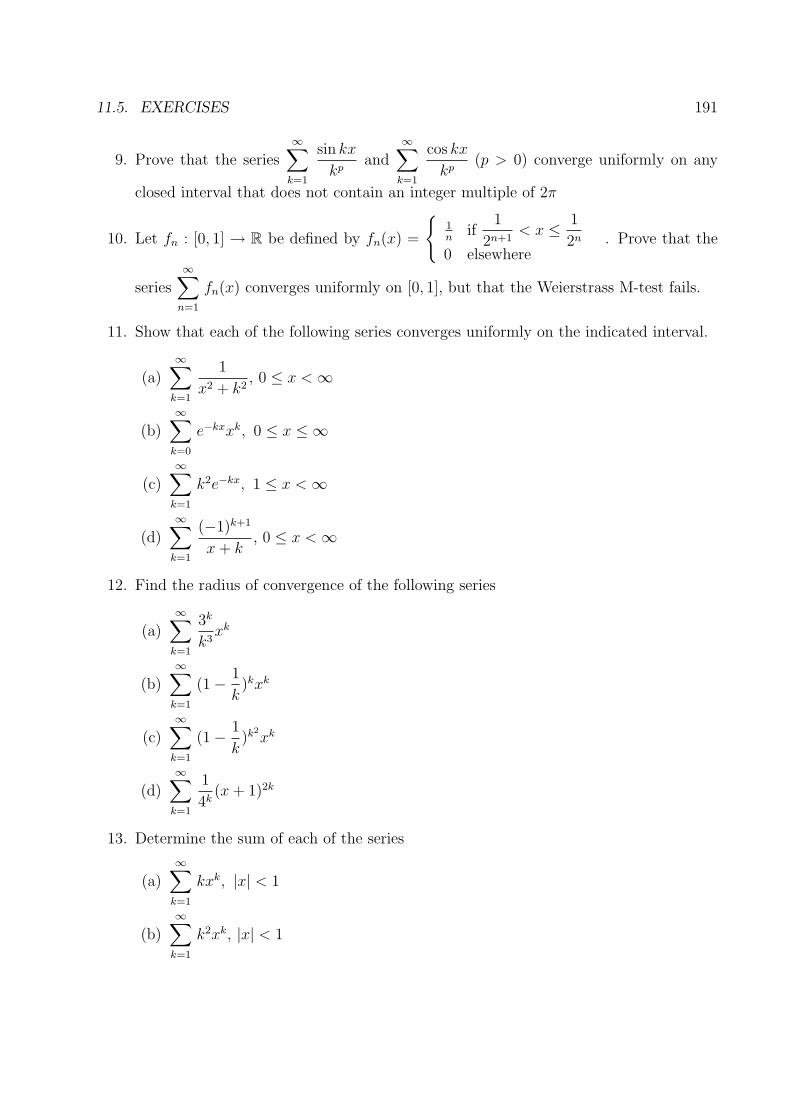
11.5. EXERCISES 191
9. Prove that the series∞∑
k=1
sin kx
kpand
∞∑k=1
cos kx
kp(p > 0) converge uniformly on any
closed interval that does not contain an integer multiple of 2π
10. Let fn : [0, 1] → R be defined by fn(x) =
{1n
if1
2n+1< x ≤ 1
2n
0 elsewhere. Prove that the
series∞∑
n=1
fn(x) converges uniformly on [0, 1], but that the Weierstrass M-test fails.
11. Show that each of the following series converges uniformly on the indicated interval.
(a)∞∑
k=1
1
x2 + k2, 0 ≤ x < ∞
(b)∞∑
k=0
e−kxxk, 0 ≤ x ≤ ∞
(c)∞∑
k=1
k2e−kx, 1 ≤ x < ∞
(d)∞∑
k=1
(−1)k+1
x + k, 0 ≤ x < ∞
12. Find the radius of convergence of the following series
(a)∞∑
k=1
3k
k3xk
(b)∞∑
k=1
(1 − 1
k)kxk
(c)∞∑
k=1
(1 − 1
k)k2
xk
(d)∞∑
k=1
1
4k(x + 1)2k
13. Determine the sum of each of the series
(a)∞∑
k=1
kxk, |x| < 1
(b)∞∑
k=1
k2xk, |x| < 1

192 CHAPTER 11. RIEMANN INTEGRAL
(c)∞∑
k=1
k
2k
(d) Let In =1∫0
(1 − x2)ndx. Show that limn→∞ In = 0.
(e) Let 0 < α < 1, and Jn =1∫α
(1 − x2)ndx. Prove that limn→∞Jn
In
= 0.
14. Let f : [a, b] × R → R be a continuous function withδf
δycontinuous on [a, b] × R. Put
F (y) =b∫a
f(x, y)dx. Show that F is differentiable on R and F ′(y) =b∫a
δ
δyf(x, y)dx.
15. Let f : [a, b] → R be continuous u, v : [c, d] → [a, b] be continuously differentiable, i.e.
u′, v′ exist and continuous on [c, d]. Put g(x) =v(x)∫u(x)
f(t)dt. Show that g is differentiable
on ]c, d[ and find g′.
16. Let f ∈ R[a, b]. Let F (x) =z∫a
f(t)dt. Show that F is the difference of two monotoneincreasing functions.
17. Let f : [0, 2π] → R be a continuous function. Assume that for each n ∈ N,
2π∫0
f(x) cos nxdx =2π∫0
f(x) sin nxdx = 0. Show that then f ≡ 0 on [0, 2π].
18. Let f : [a, b] → R be a function which is zero at all x ∈ [a, b] except at finitely many
points x1, x2, ..., xN in [a, b]. Show thatb∫a
f(x)dx = 0.
19. Let f, g : [a, b] → R be two Riemann Integrable functions such that f(x) = g(x) for all
x ∈ [a, b] except at finitely many points. Show thatb∫a
f(x)dx =b∫a
g(x)dx.
20. Let f ∈ R[−a, 0]. Show that
(a) if f is even (i.e. f(x) = f(−x)), thena∫−a
f(x)dx = 2a∫0
f(x, y)dx.
(b) if f is odd (i.e. f(−x) = −f(x)), thena∫−a
f(x)dx = 0.
21. Find F ′(x) where F is defined on [0, 1] as follows:
(a) F (x) =x∫0
dt
1 + t2
(b) F (x) =x∫0
cos t2dt

11.5. EXERCISES 193
(c) F (x) =x2∫0
cos t2dt
(d) F (x) =1∫x
√1 + t2dt
22. Let f : [a, b] → R be continuous and g ∈ R[a, b], g(x) ≥ 0 for all x ∈ [a, b]. Show that
there exists x ∈ [a, b] such thatb∫a
f(x)g(x)dx = f(c)b∫a
g(x)dx.
23. Suppose that f : [0, 1] → R is continuous. Prove that limn→∞1∫0
f(xn)dx = f(0).
194 CHAPTER 11. RIEMANN INTEGRAL

Chapter 12
The Space C(K)
1. Generalities About C (K)
2. Ascoli-Arzela Theorem
3. Stone-Weierstrass Theorem
12.1 Generalities About C (K)
Let (X, d) be any m.s , K ⊆ X a compact subset and C(K) = {f : K → R : f is continuous on K}.On C(K) we shall always put the “supremum metric”: d∞(f, g) = supx∈K |f(x) − g(x)|. Weknow that (C(K), d∞) is a complete metric space.
In this chapter we want to study some properties of this metric space. In particular we want:
a) to characterize the compact subsets of C(K)
b) to characterize the dense subsets of C(K).
12.1.1 Cantor’s Diagonal Method
Theorem 12.1.1 Let E = {x0, x1, . . . , xn, . . .} be a countable set, (X, d) a compact metricspace and fn : E → X any sequence of functions. Then, (fn)n∈N has a subsequence (fnk
)k∈N
such that for each xi ∈ E, the sequence (fnk(xi))k∈N converges in X.
Proof 12.1.2 Start with x0 and consider the sequence (fn(x0))n∈N. Since this sequencelies in the compact set X, it has a convergent subsequence, denote it (fnk,0
(x0))k∈N. Here,n0,0 < n1,0 < n2,0 < · · · < nk,0 < · · ·Now, start with the sequence (fnk,0
(x1))k∈N. As this sequence lies in the compact m.s X, ithas a convergent subsequence, denote it (fnk,1
(x1))k∈N. Here, n0,1 < n1,1 < · · · < nk,1 < · · ·Moreover, {nk,1 : k ∈ N} ⊆ {nk,0 : k ∈ N}
195

196 CHAPTER 12. THE SPACE C(K)
Next, start with the sequence (fnk,0(x2))k∈N. For the same reason this sequence has a con-
vergent subsequence, denote it (fnk,2(x2))k∈N. Here, n0,2 < n1,2 < n2,2 < · · · < nk,2 < · · · and
{nk,2 : k ∈ N} ⊆ {nk,1 : k ∈ N} ⊆ {nk,0 : k ∈ N} ⊆ · · ·In this way we get subsequences fnk,p
of fn such that (fnk,p(xp))k∈N converges and
· · · ⊆ {fnk,p: k ∈ N
} ⊆ {fnk,p−1: k ∈ N
} ⊆ · · · ⊆ {fnk,o: k ∈ N
}.
It follows that, for i ≤ p, (fnk,p(xi))k∈N converges since this is a subsequence of the convergent
subsequence (fnk,i(xi))k∈N.
Now, let (fnk,k)k∈N be the diagonal of this infinite matrix:⎛
⎜⎜⎜⎜⎜⎝
fn0,0 fn1,0 · · · fnk,0· · ·
fn0,1 fn1,1 fnk,1· · ·
.... . .
... · · ·fn0,p · · · fnk,p
· · ·...
......
...
⎞⎟⎟⎟⎟⎟⎠
Then for each xi ∈ E, except for first i terms, (fnk,k(xi))k∈N is a subsequence of (fnk,i
(xi))k∈N.So, (fnk,k
(xi))k∈N converges.
12.1.2 Pointwise and Uniformly Bounded Sets of Functions
Definition 12.1.3 Let A ⊆ X be any set and H be a set of functions f : A → R. If, foreach x0 ∈ A given, the set {f(x0) : f ∈ H} is bounded then we say that H is pointwisebounded on A. If, {f(x) : x ∈ A, f ∈ H} is bounded, then we say that H is uniformlybounded on A.
Thus, H is pointwise bounded on A ⇔ ∀x ∈ A, ∃Mx > 0 : ∀f ∈ H, |f(x)| < Mx.
H is uniformly bounded on A ⇔ ∃M > 0, ∀x ∈ A, ∀f ∈ H, |f(x)| < M.
Example 12.1.4 Let H = {fn : n ∈ N}, fn(x) =nx2
1 + nx, 0 ≤ x ≤ ∞. For any x0 ∈ [0,∞[
fixed, |fn(x)| ≤ x0 =⇒ H is pointwise bounded.
But, supn∈N, x∈[0,∞[ |fn(x)| = ∞ =⇒ H is not uniformly bounded.
Lemma 12.1.5 Let E be any set and B(E) be the space of bounded functions f : E → R,with the supremum metric d∞(f, g) = supx∈E |f(x) − g(x)|. Let fn, f ∈ B(E) be such thatd∞(fn, f) → 0 (i.e. fn → f uniformly on E). Then the set H = {fn : n ∈ N} is uniformlybounded on E.
� So “uniform boundedness” is a necessary condition for uniform convergence, but it is faraway from being sufficient. E.g. fn(x) = sin(nx) is uniformly bounded on R, but it does noteven converge pointwise.
12.1. GENERALITIES ABOUT C (K) 197
12.1.3 Equi-continuity of a set of Functions
Let A ⊆ X, x ∈ A a point and f : A → R be a function. In the definition of continuity of f
at x we have: ∀ε > 0, ∃η > 0 :
{ ∀y ∈ Ad(x, y) < η
=⇒ |f(x) − f(y)| < ε.
In this definition, η depends not only on x and ε, but also on f.
• Now, suppose that we have finitely many functions. f1, f2, . . . , fn : A → R all of them
continuous at xi. So, ∀ε > 0, ∃ηi > 0 :
{ ∀y ∈ Ad(x, y) < ηi
=⇒ |fi(x) − fi(y)| < ε.
If η = inf {η1, . . . , ηn}, then η > 0 and
{ ∀y ∈ Ad(x, y) < η
=⇒ |fi(x) − fi(y)| < ε, ∀i =
1, 2, . . . , n.
• Now, suppose that we have infinitely many fn : A → R, each of them are continuous at xi.
Hence, ∀ε > 0, ∃ηi > 0 :
{ ∀y ∈ Ad(x, y) < ηn
=⇒ |fn(x) − fn(y)| < ε.
Here inf {ηn : n ∈ N} might be zero!
Question: Is there an η > 0 that works for all fn?
Example 12.1.6 Let fn : R → R, fn(x) = cos nx, x = 0. Is there an η > 0 such that|y − 0| < η =⇒ |fn(x) − fn(y)| < ε, ∀n ∈ N?
Let us fix ε =1
2. Is there an η > 0 such that |y| < η =⇒ |cos ny − 1| <
1
2for all n ∈ N?
Let n be large enough to haveπ
n< η. Then, with y =
π
n, |cos ny − 1| = | − 2| = 2 >
1
2.
Hence, there is no η > 0 satisfying |y| < η =⇒ |fn(x) − fn(y)| < ε.
Definition 12.1.7 Let H be a set of functions f : A → R and x0 ∈ A a point. We say thatH is equi-continuous at x0 if we have:
∀ε > 0, ∃η > 0 :
{ ∀y ∈ Ad(x0, y) < η
=⇒ |f(x0) − f(y)| < ε, ∀f ∈ H.
or equivalently; ∀ε > 0, ∃η > 0 :
{ ∀y ∈ Ad(x0, y) < η
=⇒ supf∈H |f(x0) − f(y)| < ε. (Here η
depends on H but not on any particular f ∈ H)
If H is equi-continuous at every x0 ∈ A, then we say that H is equi-continuous on A.
Example 12.1.8 Let H = {f : [a, b] → R : |f(x) − f(y)| ≤ k|x − y|, ∀x, y ∈ [a, b]} , k > 0a fixed number (does not depend on f). Then H is equi-continuous on [a, b].
Indeed, ∀x ∈ [a, b], ∀ε > 0, let η =ε
k + 1, ∀y ∈ [a, b]
Then, |x − y| < η =⇒ |f(x) − f(y)| < ε, ∀f ∈ H.

198 CHAPTER 12. THE SPACE C(K)
Lemma 12.1.9 Let fn : [a, b] → R be a sequence of continuous functions. Suppose that fn
converges uniformly on [a, b] to some f : [a, b] → R. Let H = {fn : n ∈ N} . Then H isequi-continuous on [a, b].
Proof 12.1.10 Since fn → f uniformly on [a, b], we have: ∀ε > 0, ∃N ∈ N : ∀n ≥ Nsupx∈[a,b] |fn(x) − f(x)| < ε. Now, let x0 ∈ [a, b] be any point. Then
∃η > 0 :
{ ∀y ∈ [a, b]|y − x0| < η
=⇒ |fi(x0) − fi(y)| < ε, 0 ≤ i ≤ N .
Then, for this η,|x0−y| < η =⇒ |fn(x0) − fn(y)| ≤ |fn(x0) − f(x0)|+|f(x0) − f(y)|+|f(y) − fn(y)| < 3ε,
∀n ≥ N.
Hence, |x0 − y| < η =⇒ supn∈N |fn(x0) − fn(y)| < 3ε. So, H is equi-continuous on [a, b].
� So equi-continuous is a necessary condition for uniform convergence.
Lemma 12.1.11 Fix a point x ∈ K, let δx : C(K) → R be the “Dirac function”, i.e.δx(f) = f(x). Then δx is continuous.
12.2 Ascoli - Arzela Theorem
Let H ⊆ C(K) be a subset.
Theorem 12.2.1 (Main Lemma) Let D ⊆ K be a dense subset of K, fn be sequence offunctions in H. Suppose that:
1. H is equi-continuous on K.
2. For each x ∈ D, (fn)n∈N converges pointwise on D.
Then (fn)n∈N converges uniformly on K.
Proof 12.2.2 Let us see that (fn)n∈N is uniformly Cauchy on K. Let us first write what wehave:
∀x ∈ K, ∀ε > 0, ∃ηx > 0 such that
{ ∀y ∈ Kd(x, y) < ηx
=⇒ supn∈N |fn(x) − fn(y)| < ε. (1)
∀x0 ∈ D, ∀ε > 0, ∃Nx0 ∈ N such that ∀n, m ≥ Nx0 , |fn(x0) − fm(x0)| < ε. (2)
As, K ⊆ ∪x∈KBηx(x) and K is compact, there exists x1, x2, . . . , xp ∈ K such that
K ⊆ Bηx1(x1) ∪ Bηx2
(x2) ∪ · · · ∪ Bηxp(xp), for some p ∈ Z+.
As, D = K, Bηxi(xi) ∩ D �= ∅. Let xi ∈ Bηxi
(xi) ∩ D. Let N = sup{Nx1 , . . . , Nxp
}, so that
∀n, m ≥ N , |fn(xi) − fm(xi)| < ε. (3)
Let n,m ≥ N and x ∈ K be arbitrary. (So N does not depend on x).

12.2. ASCOLI - ARZELA THEOREM 199
Since, K ⊆ Bηx1(x1) ∪ Bηx2
(x2) ∪ · · · ∪ Bηxp(xp), x ∈ Bηxi
(xi) for some i ∈ {1, . . . , p} .
Then, |fn(x) − fm(x)| ≤ |fn(x) − fn(xi)| + |fn(xi) − fm(xi)| + |fm(xi) − fm(x)| < 3ε, by(1), (2), (3) above.
Hence, (fn)n∈N is uniformly cauchy on K. So, converges uniformly on K to some continuousfunction f : K → R.
Lemma 12.2.3 A pointwise bounded, equi-continuous set H ⊆ C(K) is uniformly bounded.
Proof 12.2.4 Let H ⊆ C(K) be equi-continuous on K and be pointwise bounded. So,
∀x ∈ K, ∀ε > 0, ∃ηx > 0 such that
{ ∀y ∈ Kd(x, y) < η
=⇒ supn∈N |fn(x) − fn(y)| < ε. (4)
∀x ∈ K, ∃Mx > 0 such that supf∈H |f(x)| ≤ Mx. (5)
From (4) we get that K ⊆ ∪x∈KBηx(x). As K is compact,
K ⊆ Bηx1(x1) ∪ Bηx2
(x2) ∪ · · · ∪ Bηxp(xp) for some i ∈ {1, . . . , p}.
Then for any x ∈ K, (so x ∈ Bηxi(xi)), for M = sup1≤i≤p Mxi
we have:
|f(x)| = |f(x) − f(xi) + f(xi)| ≤ |f(xi) − f(x)| + |f(xi)| ≤ Mxi+ ε ≤ M + ε.
Hence, supf∈H supx∈K |f(x)| ≤ M . (M ≥ M + ε). So, H is uniformly bounded on K.
Recall: Let (Y, d) be a complete metric space and H ⊆ Y a set. Then;
H is compact ⇐⇒{
H is totally boundedH is closed
Theorem 12.2.5 (Ascoli - Arzela) Let H be a subset of C(K). Then,
H is compact ⇐⇒⎧⎨⎩
H is equi-continuous on KH is pointwise bounded on KH is closed in C(K)
Proof 12.2.6 (⇒) Assume that H is compact. So, it is closed and totally bounded.
Hence, ∀ε > 0, ∃f1, . . . , fp ∈ H : H ⊆ Bε(f1)∪· · ·∪Bε(fp). Since any finite set of continuousfunctions is equi-continuous,
∀x ∈ K, ∃ηx > 0 such that
{ ∀y ∈ Kd(x, y) < ηx
=⇒ sup1≤i≤p |fi(x) − fi(y)| < ε. (6)
Now, let f be arbitrary, say f ∈ Bε(fi). So, supy∈K |f(y) − fi(y)| < ε. (7)
So,
{ ∀y ∈ Kd(x, y) < ηx
=⇒ |f(x) − f(y)| ≤ |f(x) − fi(x)|+ |fi(x) − fi(y)|+ |fi(y) − f(y)| < 3ε.
Hence, H is equi-continuous on K.
Next, for x ∈ K fixed, let δx : C(K) → R be the mapping defined by δx(f) = f(x). This δx
is a continuous mapping. Hence, δx(H) is compact in R, so bounded. But,δx(H) = {f(x) : f ∈ H}. So H is pointwise bounded on K.

200 CHAPTER 12. THE SPACE C(K)
(⇐) Conversely, suppose that the 3 conditions of the theorem are satisfied. As, K is acompact metric space and every compact metric space is separable, K has a countable densesubset ε = {x0, . . . xn, . . .} with ε = K. Also, H is equi-continuous and pointwise boundedon K. By lemma 12.2.3 H is uniformly bounded, i.e. ∃M > 0 such that ∀x ∈ K, ∀f ∈ H,f(x) ∈ [−M,M ].
Let now (fn)n∈N be a sequence in H. (fn)n∈N has a subsequence (fnk)k∈N that converges
pointwise on ε. As, (fnk)k∈N ∈ H by lemma 12.2.1 (fnk
)k∈N converges uniformly to somef ∈ H since H is closed. Thus, every sequence fn in H has a convergent subsequence.
Hence, H is compact.
Theorem 12.2.7 Let fn : [a, b] → R be sequence of functions such that f ′n exists and
|f ′n(x)| ≤ M, ∀x[a, b]. Also assume that (fn(a))n∈N is bounded. Then for x, y ∈ [a, b],
|fn(x) − fn(y)| ≤ f ′(c)|x − y| ≤ M |x − y|, for some c ∈]x, y[. Hence, (fn)n∈N is equi-continuous on [a, b].
Also, |fn(x)| = |fn(x) − fn(a) + fn(a)| ≤ |fn(x) − fn(a)|+ |fn(a)| ≤ M(b−a)+ |fn(a)| ≤ M .
Hence, (fn)n∈N is pointwise bounded. So (fn)n∈N has a uniformly convergent subsequence.
Example 12.2.8 Let fn : [0, 1] → R be a pointwise convergent sequence and |f ′n(x)| ≤ 1.
Then, (fn)n∈N converges uniformly.
Indeed, let fn → f pointwise on [0, 1] So in particular (fn(0))n∈N is bounded. Hence, by thepreceding example fn has a subsequence that converges uniformly on [0, 1] to f . This showsthat f is the only cluster point of fn. Since fn belongs to a compact set H = {fn : n ∈ N} ,fn → f uniformly on [0, 1].
12.3 Stone - Weierstrass Theorem
In this section we are looking for dense subsets of C(K). First consider the space (C([0, 1]), d∞)
• Let A be the set of all the polynomial functions P : [0, 1] → R. Since every polynomial iscontinuous, A ⊆ C([0, 1]). Properties of A:
1. A is a vector space over R
2. A is a ring
3. A has a unit element 1
4. ∀x0 �= y0 x0, y0 ∈ [0, 1], ∃P ∈ A : P (x0) �= P (y0).
Weierstrass Approximation Theorem says that A = C([0, 1]).
• Now, let B =
{n∑
k=0
ckenkx : nk ∈ N, ck ∈ R, 0 ≤ x ≤ 1
}. Then,

12.3. STONE - WEIERSTRASS THEOREM 201
1. B is a vector space over R
2. B is a ring
3. B has a unit element 1
4. ∀x0 �= y0, x0, y0 ∈ [0, 1]∃f ∈ B : f(x0) �= f(y0)
• Now, let C =
{(a0 +
n∑k=0
ak cos kx + bk sin kx) : n, k ∈ N, ak, bk ∈ R, 0 ≤ x ≤ 2π
}. Then,
1. C is a vector space over R
2. C is a ring
3. C has a unit element 1
4. ∀x0 �= y0, x0, y0 ∈ [0, 1], ∃f ∈ C : f(x0) �= f(y0).
• Now, let ϕ : [0, 1] → R be a continuous, strictly increasing function. D =
{n∑
k=0
akϕk(x) : ak ∈ R, k ∈ N
Then,
1. D is a vector space over R
2. D is a ring
3. D has a unit element 1
4. ∀x0 �= y0, x0, y0 ∈ [0, 1], ∃f ∈ D : f(x0) �= f(y0)
Definition 12.3.1 A subset A of C(K) is said to be an algebra if it is both a vector spaceand a ring. In other words,
1. ∀f, g ∈ A, ∀d, u ∈ R : d · f + u · g ∈ A.
2. ∀f, g ∈ A, f · g ∈ A.
If also 1 ∈ A then we say that A is unital.If ∀x �= y, ∃f ∈ A : f(x) �= f(y), then we say that A separates the points of K.
In the above examples A,B,C,D are unital subalgebras that separate the points of [0, 1].
Lemma 12.3.2 Let A be a unital subalgebra of C(K). Then for f ∈ A, |f | ∈ A, too.

202 CHAPTER 12. THE SPACE C(K)
Proof 12.3.3 Let f ∈ A. Let M = supx∈K |f(x)|. Thenf(x)
M∈ [−1, 1]. We know that the
set of polynomials is dense in C([−1, 1]).
Let h(x) = |x| ∈ C([−1, 1]). Then, ∀ε > 0, ∃pn(x) = anxn + · · · + a0 a polynomial such thatsup|x|<1 |p(x) − |x|| < ε.
Then the function p
(f(x)
M
)= an
(f(x)
M
)n
+ · · · + a1f(x)
M+ a0 ∈ A since A is a unital
algebra. Then, sup|x|<1
∣∣∣∣p(
f(x)
M
)− |f(x)|
M
∣∣∣∣ < ε. Hence,|f(x)|
M∈ A =⇒ |f | ∈ A.
Corollary 12.3.4 Let A be a unital subalgebra of C(K). Then, for any f, g ∈ A : sup {f, g}and inf {f, g} are in A.
Proof 12.3.5 sup {f, g} =|f − g| + f + g
2, inf {f, g} =
f + g − |f − g|2
. Hence by lemma
12.3.2 sup {f, g} and inf {f, g} are in A.
Lemma 12.3.6 Let A be a unital subalgebra of C(K) separating the points of K. Then for
each x �= y (x, y ∈ K), for each α, β ∈ R, there is ϕx,y ∈ A such thatϕx,y(x) = αϕx,y(y) = β
Proof 12.3.7 Let x �= y and α, β ∈ R be given. Since A separates the points of K, there is
an f ∈ A such that f(x) �= f(y). Let ϕx,y = α + (β − α)f − f(x)
f(y) − f(x). Then, ϕx,y ∈ A and
ϕx,y(x) = αϕx,y(y) = β
Theorem 12.3.8 (Stone - Weierstrass) Any unital subalgebra A of C(K) separatingthe points of K is dense in C(K).
Proof 12.3.9 Let A be a unital subalgebra of C(K) separating the points of K.
Let f ∈ C(K) and ε > 0 be given. We have to show that there is g ∈ A such thatsupx∈K |f(x) − g(x)| < ε. Let x ∈ K be given. Then for each y ∈ K, there is a ϕx,y ∈ Asuch that ϕx,y(x) = f(x), ϕx,y(y) = f(y)
As ϕx,y(y) = f(y), ϕx,y(y) < f(y) + ε. Hence, since both ϕx,y and f are continuous at y,there is ηy > 0 such that ∀z ∈ K ∩ Bηy(y) : ϕx,y(z) < f(z) + ε. As K ⊆ ∪y∈KBηy(y),K ⊆ Bηy1
(y1) ∪ · · · ∪ Bηyk(yk), for some y1, y2, . . . yk ∈ K.
Hence, ∀z ∈ Bηyi(yi) ∩ K : ϕx,y(z) < f(z) + ε and ϕx,yi
(x) = f(x).
Let ψx = sup {ϕx,y1 , . . . , ϕx,yk}. Then by corollary 12.3.4, ψx ∈ A and ∀z ∈ K,
ψx(z) < f(z) + ε, ψx(x) = f(x).
From ψx(x) = f(x) > f(x) − ε, by continuity of ψx and f , there is an ηx > 0 such that∀z ∈ Bηn(x) ∩ K, ψx(z) > f(z) − ε. Hence, from K ⊆ ∪x∈KBηn(x), we get;

12.3. STONE - WEIERSTRASS THEOREM 203
K ⊆ Bηx1(x1) ∪ · · · ∪ Bηxp
(xp).
So, there are ψx1 , . . . , ψxp ∈ A such that ψxi(z) > f(z) − ε, ψxi
(z) < f(z) + ε, ∀z ∈ K.
Let g = inf{ψx1 , . . . , ψxp
}. Then g ∈ A and ∀z ∈ K, f(z) − ε < g(z) < f(z) + ε, i.e.
supx∈K |f(x) − g(x)| < ε. This proves that A is dense in C(K). So, A = C(K).
Example 12.3.10 Let A0 =
{a0 +
n∑k=0
(ak cos kx + bk sin kx) : ak, bk ∈ R, k ∈ N
}. Consider
A0 as a subset of C([0, 2π]). Then A0 is a unital subalgebra of C([0, 2π]). A0 separates allpair of points in [0, 2π] except 0 and 2π.
Let C∗([0, 2π]) = {f ∈ C([0, 2π]) : f(0) = f(2π)} = {f ∈ C([0, 2π]) : f is periodic with 2π period}.Now, let K = {z ∈ C : |z| = 1} and consider C(K). Let ϕ : [0, 2π] → K, ϕ(t) = (cos t, sin t).Let T : C(K) → C∗([0, 2π]), T (f) = f ◦ ϕ. Then T is continuous and onto.
Let A = {p(z) : p is a polynomial} . A ⊆ C(K), A is a unital subalgebra and separates thepoints of K. Hence, A = C(K).
Now, if we identify z ∈ K, with z = (cos x, sin x), then
T (A) =
{a0 +
n∑k=0
(ak cos kx + bk sin kx) : ak, bk ∈ R, k ∈ N
}= A0.
Hence, since A is dense in C(K) and T is onto, A0 is dense in C∗([0, 2π]).
Thus, if f : [0, 2π] → R is continuous and 2π periodical then there exists a sequence of
trigonometric polynomials, Pn(x) = a0 +n∑
k=0
(ak cos kx + bk sin kx) that converges uni-
formly to f.
Theorem 12.3.11 The metric space (C(K), d∞) is separable.
Proof 12.3.12 We know that:
1. Every compact m.s is separable.
2. Every separable m.s is second countable, i.e. there exists a sequence (βn)n∈N of opensets such that any other open set is a union of some of these βn’s.
So, let (βn)n∈N be such a sequence for the m.s (K, d). For each n ∈ N let fn(x) = d(x, βcn).
(x ∈ K, βn ⊆ K, βcn = K\βn) Then, fn is continuous and for any x �= y (x, y ∈ K) for some
n ∈ N, (fn(x) �= fny). Let E = {1, f0, f1, . . . , fn, . . .} and A be the subalgebra generated byE.
A typical element of A is of the form: g =∑
an,p,q,...,rfn1 , f p
2 , . . . , f rk . Then by Stone -
Weierstrass Theorem A is dense in C(K). Let, B be the set of the same type of elements asin A but with rational coefficients. Then, B is dense in A. So, B is dense in C(K). As Bis countable, C(K) is separable.

204 CHAPTER 12. THE SPACE C(K)
Warning: If K is topologically compact but not metric, then C(K) is in general is notseparable.

12.4. EXERCISES 205
12.4 Exercises
1. Let (K, d) be a compact metric space and C(K) = {f : K → R: f is continuous }(a) Let (fn)n∈N be a uniformly convergent sequence in C(K). Show that the set
H = {fn : n ∈ N} is uniformly bounded and equi-continuous at each x ∈ K.
(b) Let H be an equi-continuous subset of C(K). Show that H is also equi-continuouson K.
(c) Let x0 ∈ K, H ⊆ C(K) be equi-continuous on K and H(x0) = {f(x0) : f ∈ H}be bounded. If K is connected, show that then H is uniformly bounded.
(d) Let (fn)n∈N be a sequence in C(K), x0 ∈ K and xn → x0. If {fn : n ∈ N} is aequi-continuous at x0 and fn(x0) → f(x0). Show then fn(xn) → f(x0).
2. Let H = {f ∈ C[0, 1] : f ′ exists and |f(x)|+ |f ′(x)| ≤ 1 ∀ x ∈ [0, 1]}. Show that everysequence (f)n∈N in H has a uniformly convergent subsequence.
3. Let H ⊆ C(K), E ⊆ K be dense in K and H be equi-continuous at each x ∈ E. Showthat
(a) ∀ η > 0 K ⊆ ∪x∈EBη(x)
(b) H is also equi-continuous on K.
4. Let (K, d) be a compact metric space. For a subset F of K, let
I(F ) = {f ∈ C(K) : f(F ) = {0}}. Show that;
(a) I(F ) is a closed ideal of C(K)
(b) I(F ) = I(F )
(c) F1 ⊆ F2 → I(F2) ⊆ I(F1).
5. Let I be a closed ideal of C(K) and F = {x ∈ K : ∀ f ∈ I, f(x) = 0}, i.e.
F = ∩f∈If−1({0}). Show that F is closed and I ⊆ C(K) iff ∩f∈If
−1({0}) = ∅6. Let I be a closed ideal of C(K). Show that I = C(K) iff ∩f∈If
−1({0}) = ∅.
7. Let A be a subalgebra of C(K). Show that if◦A�= ∅ then A = C(K)
8. Let f ∈ C[0, 1]. If, for each n ∈ N,1∫0
xnf(x)dx = 0 then f ≡ 0 on [0, 1].
9. Let C∗[0, 2π] = {f ∈ C(K) : f(0) = f(2π)} and
A = {n∑
k=0
(ak cos kx + bk sin kx) : x ∈ [0, 2π], n ∈ N, ak, bk ∈ R} Show that A is a
subalgebra of C∗[0, 2π] and A is dense in it.

206 CHAPTER 12. THE SPACE C(K)
10. Let f ∈ C∗[0, 2π]. If1∫0
f(x) sin nxdx =2π∫0
f(x) cos nxdx = 0. Show that then f ≡ 0 on[0, 2π].
11. Let A = {n∑
k=1
fk(x)gk(y) : fk, gk ∈ C[0, 1], n ∈ N}. Show that A is dense in C([0, 1] ×[0, 1]).

Chapter 13
Baire Category Theorem
1. Generalities
2. Basic Notations
3. Various Forms of the Baire Category Theorem
4. Baire’s Great Theorem Without Proof
5. Applications
13.1 Generalities
Let (X, d) be a metric space, fn : X → R be sequence of continuous functions.
Suppose fn converges pointwise on K to some function f . We know that f need not becontinuous.
What does “f is not continuous” mean? Does it say that f is discontinuous everywhere?
Questions:
1. How discontinuous is this f?
2. Given g : X → R how to recognize that g is the pointwise limit of a sequence ofcontinuous functions (gn)n∈N?
Example 13.1.1 Let f : R → R, f(x) =
{1 if x ∈ Q0 if x ∈ R \ Q
Question: Is there a sequence fn : R → R of continuous functions such that ∀x ∈ R,f(x) = limn→∞ fn(x)? (not possible)
Example 13.1.2 Let f : R → R be the derivative of some g : R → R. Then, ∀x ∈ R,
f(x) = limn→∞g(x + 1
n
)− g(x)1n
= fn(x), i.e. limn→∞ fn(x) = f(x). (each fn is continuous)
207

208 CHAPTER 13. BAIRE CATEGORY THEOREM
Definition 13.1.3 Let B1(x) be the set of the functions f : X → R, such thatf(x) = limn→∞ fn(x), ∀x ∈ X for some sequence of continuous functions fn : X → R. Thefunctions that belong to B1(x) are said to be Baire-1 functions.
Similarly we define B2(x) = {g : X → R : g(x) = limn→∞ fn(x) for some fn ∈ B1(x)} .
B3(x) = {h : X → R : h(x) = limn→∞ fn(x) for some gn ∈ B2(x)}....
So, the above questions become:
1. How discontinuous a Baire-1 function may be?
2. Given a function f : X → R, how to recognize it is a Baire-1 function or not?
Thus, our task in this chapter is to characterize Baire-1 functions.
13.2 Basic Notations
13.2.1 Gδ-sets, Fσ-sets
Let (X, d) be a metric space.
Definition 13.2.1 A set A ⊆ X is said to be a Gδ-set, if it is possible to present A as anintersection countably many open sets On, i.e. A = ∩n∈NOn.
A set B ⊆ X is said to be a Fσ-set if it is possible to present B as a union of countablymany closed sets Fn. i.e., B = ∪n∈NFn.
Example 13.2.2 1. In any m.s (X, d), every open set is a Gδ-set and every closed set isa Fσ-set.
2. A is a Gδ-set ⇐⇒ Ac is a Fσ-set.
3. Let X = R. Then,[a, b] = ∩n≥1
]a − 1
n, a + 1
n
[{a} = ∩n≥1
]a − 1
n, a + 1
n
[]a, b[= ∪n≥1
[a + 1
n, b − 1
n
] .
Question Q is a Fσ-set. Is Q a Gδ-set?
13.2.2 Nowhere Dense Sets
Let (X, d) be a metric space.
Definition 13.2.3 A set A ⊆ X is said to be nowhere dense if◦
(A)= ∅.

13.2. BASIC NOTATIONS 209
Example 13.2.4 In R, A = N, A = Z are nowhere dense. But Q is not nowhere dense.
Example 13.2.5 Let X = R2, A = R×{0}. Then A is closed in R2 and◦A= ∅. So, R×{0}
is nowhere dense in R2.
Example 13.2.6 A closed set F ⊆ X is nowhere dense iff X \ F = X. Recall for any
A ⊆ X,( ◦A)c
= (Ac) and(A)c
=◦
(Ac)
Example 13.2.7 For any closed set F ⊆ X, A = ∂F = F\ ◦F is nowhere dense.
For any open set B ⊆ X, A = ∂B = B \ B is nowhere dense.
Example 13.2.8 The union of finitely many nowhere dense sets is nowhere dense. A subsetof a nowhere dense set is nowhere dense.
13.2.3 First and Second Category Sets, Residual Sets
Let (X, d) be a metric space and M ⊆ X a set.
Definition 13.2.9 We say that “M is of the first category in X” if it is possible topresent M as a countable union of nowhere dense sets.
Example 13.2.10 In R, Q is of the first category. Q =∞∪k=1 Ak, Ak =
1
kZ. Then Ak is
closed and◦
Ak= ∅.In R, any countable set is of the first category.
Warning To be of the “first category” is a relative notion. e.g. N as a subset of R isof the first category, but if we consider N as a metric space of its own with the metricd(n,m) = |n − m|, then N is discrete and N is not of the first category in itself.
Example 13.2.11 If M0,M1, . . .Mn, . . . ⊆ X are of the first category in X, then the union
M = ∪n∈NMn is also of the first category in X. Indeed, if Mn = ∪k∈N An,k with◦
An,k= ∅,then M = ∪(n,k)∈N×NAn,k and
◦An,k= ∅, ∀(n, k) ∈ N × N.
Definition 13.2.12 A subset M of a metric space (X, d) is said to be of the second cat-egory in X, if M is not of the first category in X. Thus, a subset M of X is either of thefirst category or of the second category in X.
Definition 13.2.13 A subset M of a metric space (X, d) is said to be a residual set iffX \ M is of the first category in X.

210 CHAPTER 13. BAIRE CATEGORY THEOREM
13.3 Various Forms of the Baire Category Theorem
Theorem 13.3.1 A complete metric space (X, d) is of the second category in X, i.e. if we
write X as ∪n∈NAn for some sets An, then for at least one n ∈ N,◦
An �= ∅.
Proof 13.3.2 Suppose that for some sets An ⊆ X, we have ∪n∈NAn = X and ∀n ∈ N◦
An= ∅.Since ∪n∈NAn = X, ∪n∈NAn = X, too. Then, since
◦An= ∅, the open set On = X \ An is
dense in X. So, it is enough to prove the following lemma.
Lemma 13.3.3 Let (X, d) be a complete m.s and On’s are open, dense sets. Then the setD = ∩n∈NOn is a dense Gδ-set.
Proof 13.3.4 We have to prove that ∀x ∈ X, ∀ε > 0 : Bε(x) ∩ D �= ∅.Fix an x ∈ X and an ε > 0. As O0 = X, Bε(x) ∩ O0 �= ∅. As, Bε(x) ∩ O0 is open, for anyx0 ∈ Bε(x)∩O0 there is ε0 > 0 such that B′
ε0(x0) ⊆ Bε(x)∩O0. We can and do assume that
ε0 <ε
2.
Since O1 = X, Bε0(x0) ∩ O1 �= ∅. Hence for any x1 ∈ Bε0(x0) ∩ O1, there is ε1 <ε0
2such
that B′ε1
(x1) ⊆ Bε0(x0) ∩ O1.
As O2 = X, Bε0(x0) ∩ O2 �= ∅. Hence for any x2 ∈ Bε0(x0) ∩ O2, there is ε2 <ε1
2such that
B′ε2
(x2) ⊆ Bε1(x1) ∩ O2, . . . etc.
In this way we get sets Bεn(xn) such that
i ) Bε(x) ⊇ B′ε0
(x0) ⊇ · · · ⊇ B′εn
(xn) ⊇ · · · and εn <ε
2n→ 0.
ii ) B′εn
(xn) ⊆ B′εn−1
(xn−1) ∩ On.
Hence, (X, d) being complete, by “Cantor’s Nested Interval” theorem:∩k∈NB′
εk(xk) �= ∅.
Let y ∈ ∩k∈NB′εk
(xk) be any point. Then by (ii), y ∈ On, ∀n ∈ N and by (i) y ∈ Bε(x).Then, y ∈ Bε(x) ∩ D. Hence, Bε(x) ∩ D �= ∅ and D is dense in X.
Example 13.3.5 The set M = R \ Q is of the second category in R.Indeed, we know that:i) Q is of the first category in R.ii) The union of two first category sets is of the first category.
So, if R \ Q was of the first category in R, then since R = Q ∪ (R \ Q) , Q would also be ofthe first category in R.
Example 13.3.6 The space (C(K), d∞) is of the second category in itself.
Another form of theorem 13.3.1 is this:

13.3. VARIOUS FORMS OF THE BAIRE CATEGORY THEOREM 211
Theorem 13.3.7 Let (X, d) be a complete m.s. If for some closed sets Fn’s, we have
X = ∪n∈NFn, then the set ∪n∈N
◦(Fn) is dense in X.
Proof 13.3.8 Let An = ∂Fn = Fn\◦
Fn. We know that An is closed and◦
An= ∅. Hence,On = X \ An is a dense open set. So, by lemma 13.3.3 ∩n∈NOn is dense in X.
Let us see that ∩n∈NOn ⊆ ∪n∈N
◦(Fn). Let x ∈ ∩n∈NOn be any point. Hence, x ∈ On, ∀n ∈ N.
Now, since X = ∪n∈NFn, x ∈ Fp for some p ≥ 0. As,
{x ∈ Op
x ∈ Fp=⇒
{x /∈ Ap
x ∈ Fp=⇒ x ∈
◦Fp .
Hence, ∩n∈NOn ⊆ ∪n∈N
◦(Fn).
These three results (13.3.1,13.3.3,13.3.7) are known as “Baire Category Theorems”.
Theorem 13.3.9 In any complete metric space (X, d) :
1. Every residual set is of the second category in X.
2. Every dense Gδ − set is of the second category in X.
Proof 13.3.10 1. Let M ⊆ X be a residual set, i.e. X \M is of the first category in X.If M was of the first category in X, M ∪ X \ M = X would be of the first category inX, too, which is not possible since (X, d) is complete.
2. Let M be a dense Gδ-set. Let us see that M is residual, i.e. X \ M is of the firstcategory. Now, since M is a Gδ-set, M = ∩n∈NOn for some open sets On’s. Since,M ⊆ On, each On is dense in X.
Hence, Fn = X \On is a closed nowhere dense set. So, ∪n∈NFn = X \M is of the firstcategory in X.
Example 13.3.11 1. In R, M = R \ Q is a residual set.
2. In R, Q is NOT a Gδ-set.
3. In any complete m.s (X, d), any set M ⊆ X such that◦
M �= ∅ cannot be of the firstcategory in X.
Proposition 13.3.12 In a complete metric space (X, d), if M is of the first category, thenX \ M = X.
Proof 13.3.13 As M is of the first category in X, M = ∪n∈NAn with◦
An= ∅, ∀n ∈ N.Hence, by lemma 13.3.3, with On = X \ An, D = ∩n∈NOn is dense in X. But, M ∩ D = ∅.So, we have
◦M= ∅.
Example 13.3.14 1. In a complete m.s. (X, d), a set M ⊆ X and its complement M c
both may be of the second category in X.
2. In a complete m.s. (X, d), any set M containing a second category set is of the secondcategory.

212 CHAPTER 13. BAIRE CATEGORY THEOREM
13.4 A Study of Discontinuous Functions (Baire’s Great
Theorem)
Let f : R → R be the “Riemann function”, i.e. f(x) =
⎧⎪⎪⎨⎪⎪⎩
0 if x ∈ R \ Q1 if x = 01
nif x ∈ Q
Then f is continuous at every x ∈ R \ Q and discontinuous at every x ∈ Q. Hence,Cf = {x ∈ R : f is continuous at x} = R \ Q, a Gδ-set.
Question: Let (X, d) be a m.s f : X → R be an arbitrary function andCf = {x ∈ X : f is continuous at x} . What is the structure of Cf ?
Theorem 13.4.1 For any metric space (X, d), for any f : X → R, Cf is a Gδ − set. (maybe ∅)
Proof 13.4.2 Let f : X → R, f(x) = arctan (f(x)). Since, arctan : R →]−π
2,π
2
[is a
homeomorphism, f is continuous at a point x ∈ X ⇐⇒ f is continuous at x. The advantageof f over f is f is bounded. So, if necessary replacing f by f , we can assume that f isbounded.
Definition 13.4.3 For any set A ⊆ X, A �= ∅, let O(f, A) = supx∈A(f(x)) − infx∈A(f(x)).This quantity is said to be the oscillation of f on A.
Clearly, B ⊆ A =⇒ O(f, B) ≤ O(f, A).
Fix a point x0 ∈ X. Let O(f, x0) = limn→∞ O(f, B 1n(x0)). This limit exists. The number is
said to be the oscillation of f at x0.
Proposition 13.4.4 ∀α > 0, the set Aα = {x ∈ X : O(f, x) < α} is an open set.
Proof 13.4.5 Let x0 ∈ A be any point. So O(f, x0) < α. Hence, there is n > 1 such thatO(f, B 1
n(x0)) < α. Then, B 1
n(x0) ⊆ Aα. Hence, Aα is open.
Theorem 13.4.6 The function f is continuous at a point x0 ∈ X iff O(f, x0) = 0.
Conclusion: Cf is a Gδ-set.Cf = {x ∈ X : f is continuous at x}
= {x ∈ X : O(f, x) = 0}= ∩n≥1
{x ∈ X : O(f, x) < 1
n
}Example 13.4.7 • Let f : R → R, f(x) =
{1 if x ∈ Q0 if x ∈ R \ Q
. Then, Cf = ∅.• If f : R → R, f(x) = sin x, then Cf = R.• But we know that Q is not a Gδ-set. So, there is no f : R → R such that Cf = Q.
13.4. A STUDY OF DISCONTINUOUS FUNCTIONS (BAIRE’S GREAT THEOREM)213
Question Given a Gδ-set, A ⊆ R, is there a function such that Cf = A?
Theorem 13.4.8 Let (X, d) be a metric space. Suppose that there exists a set M ⊆ X suchthat M = M c = X (i.e. X = R, M = Q) Let A be any Gδ-set. Then there exists a functionf : X → R such that Cf = A.
Proof 13.4.9 Since A is a Gδ-set, Ais of the form: A = ∩n∈NOn, where On’s are open. LetO0 = X and replacing On by O1 ∩ · · · ∩ On we can assume that O0 ⊇ O1 ⊇ · · · ⊇ On ⊇ · · ·so that ∩n∈NOn = A and A ⊆ On, ∀n ∈ N.
Then, X = A ∪ (O0 \ O1) ∪ (O1 \ O2) ∪ · · · ∪ (On \ On+1) ∪ · · · Any two of these sets aredisjoint. Then each x ∈ X belongs to only one of these sets. Now, define a function asfollows: Let x ∈ X be any point.
• If x ∈ A, let f(x) = 0.
• If x /∈ A, then x ∈ On \ On+1, for some n ∈ N. There are cases:
(i) x ∈ M ∩ (On \ On+1). In this case put f(x) =1
n + 1.
(ii) x ∈ M c ∩ (On \ On+1) . In this case put f(x) = − 1
n + 1.
Let us see that Cf = A. To see this, let first a ∈ A be a point and xn ∈ X be any sequenceconverging to a.
We have to show that f(xn) → f(a) = 0. If xn ∈ A for all but finitely many n ∈ N, thenf(xn) = 0 → f(a).
Otherwise, since a ∈ A = ∩n∈NOn, a ∈ Op, ∀p ∈ N. As, Op is open, xn ∈ Op, for all butfinitely many n ∈ N.
Hence, each Op \ Op+1 contains xn, for only finitely many n ∈ N.
Hence, f(x) = ± 1
n + 1→ 0 = f(a), as n → ∞. Then, A ⊆ Cf . Now, suppose a /∈ A. Then,
a belongs to one and only one Op \ Op+1. So, f(a) = ± 1
p + 1.
If a ∈ (Op \ Op+1) ∩ M, then let xn ∈ M c be such that xn → a. Then, f(xn) ≤ 0. So,
f(xn) �1
p + 1.
If a ∈ (Op \ Op+1) ∩ M c, then f(a) = − 1
p + 1.
Then, let xn ∈ M : xn → a. Then f(xn) ≥ 0. So, f(xn) � − 1
p + 1. Hence, f is discontinuous
at every a /∈ A. So, Cf = A.
13.4.1 Continuity of Baire-1 Functions
Let (X, d) be a metric space. fn : X → R be a sequence of continuous functions. Supposethat, for each x ∈ X, (fn(x))n∈N converges to some f : X → R, i.e. fn → f pointwise on X.
214 CHAPTER 13. BAIRE CATEGORY THEOREM
Question: What is Cf ?
Let, for n ∈ N and k = 1, 2, . . ., An(k) = supp∈N
{x ∈ X : |fn+p(x) − f(x)| ≤ 1
k
}.
Theorem 13.4.10 1. Cf =∞∩k=1 ∪n∈N
◦An (k)
2. If (X, d) is complete, then Cf is residual. (i.e., a dense Gδ-set)
Proof 13.4.11 1. Let B =∞∩k=1 ∪n∈N
◦An (k). Let x0 ∈ B be a point. We want to show
that f is continuous at x0. Let ε > 0 be arbitrary. Then choose k ≥ 1 such that1
k<
ε
3.
Since, for this k, x0 ∈ ∪n∈N
◦An (k), x0 ∈
◦An0 (k), for some n0 ∈ N.
Hence, there is ηk > 0 such that Bηk(x) ⊆
◦An0 (k).
So, ∀x ∈ Bηk(x), |fn0+p(x) − f(x)| ≤ 1
k. In particular, |fn0+p(x0) − f(x0)| <
1
k.
Now, since fn(x0) → f(x0), there is p ∈ N such that |fn0+p(x0) − f(x0)| ≤ 1
k. (1)
As fn0+p is continuous at x0, there is η < ηk such that ∀x ∈ Bη(x0) :
|fn0+p(x) − fn0+p(x0)| ≤ 1
k. (2)
Then, for x ∈ Bη(x0),
|f(x) − f(x0)| ≤ |f(x) − fn0+p(x)| + |fn0+p(x) − fn0+p(x0)| + |fn0+p(x0) − f(x0)| ≤ 3
k.
Hence, B ⊆ Cf .
• Conversely, let x0 ∈ Cf and let k ≥ 1 be any number. Since fn(x0) → f(x0), for
some n ∈ N, |fn(x0) − f(x0)| ≤ 1
2k. Now the function gn = fn − f is continuous at x0
and |gn(x0)| ≤ 1
2k. So, there is η > 0 such that ∀x ∈ Bη(x0), |gn(x)| ≤ 1
k. This says
that, Bη(x0) ⊆ An(k). So, x0 ∈◦
An (k) =⇒ x0 ∈ ∪n∈N
◦An (k). This being true for any
k ≥ 1, x0 ∈∞∩k=1 ∪n∈N
◦An (k). Thus, Cf ⊆ B.
Hence, B = Cf .
2. Now, let for all k ≥ 1, n ∈ N Bn(k) =
{x ∈ X : supp∈N |fn+p(x) − f(x)| ≤ 1
k
}Clearly Bn(k) ⊆ An(k).
Moreover, Bn(k) = ∩p∈N
{x ∈ X : |fn+p(x) − f(x)| ≤ 1
k
}. So, Bn(k) is closed since
fn+p and fn are continuous.

13.4. A STUDY OF DISCONTINUOUS FUNCTIONS (BAIRE’S GREAT THEOREM)215
Moreover, since for each x ∈ X, fn(x) converges, so it is Cauchy, so x ∈ Bn(k) forsome n ∈ N.
Hence, ∪n∈NBn(k) = X. By lemma 13.3.3⋃
n∈N
( ◦Bn (k)
)is dense in X.
So, since⋃
n∈N
( ◦Bn (k)
)⊆ ⋃n∈N
◦An (k), Ok =
⋃n∈N
◦An (k) is open and dense in X.
Hence, Cf = ∩k≥1Ok is a dense Gδ-set.
Example 13.4.12 Let f : R → R, f(x) =
{1 if x ∈ Q0 if x ∈ R \ Q
Is there a sequence of continuous functions fn : R → R that converges pointwise to f on R?i.e., is f a Baire-1 function?
As, Cf = ∅, f is not a Baire-1 function. But, ∀x ∈ R, f(x) = limn→∞ limm→∞ [cos(m!xπ)]2n .So, f is a Baire-2 function.
Question: Given a function f : X → R how to recognize that f is a Baire-1 function?
Theorem 13.4.13 (Baire’s Great Theorem) Let (X, d) be a complete metric space andf : X → R be a given function. Then, f is Baire-1 ⇐⇒ ∀F ⊆ X, closed, the restrictionfunction f|F : F → R is continuous at least at one point x0 ∈ F. (i.e. ∃fn : X → Rcontinuous, fn → f pointwise ⇐⇒ ∀F ⊆ X, ∀xn ∈ F, xn → x0 =⇒ f(xn) → f(x0))

216 CHAPTER 13. BAIRE CATEGORY THEOREM
13.5 Exercises
Let (X, d) be a metric space.
1. A function f : X → R is said to be lsc(= lower semi-continuous) at a point x0 ∈ Xif
∀ ε > 0 ∃ η > 0 ∀x ∈ Bη(x0), f(x) > f(x) − ε
usc(= upper semi-continuous) at x0 if
∀ ε > 0 ∃ η > 0 ∀x ∈ Bη(x0), f(x) < f(x) + ε
(a) Show that f is usc at x0 iff −f is lsc at x0
(b) f is continuous at x0 iff both usc and lsc at x0.
(c) f is usc at every x ∈ X iff ∀ a ∈ R, the set f−1(]−∞, a[) is open in X.
(d) f is lsc at every x ∈ X iff ∀ a ∈ R, the set f−1(]a,∞[) is open in X.
(e) Let A ⊆ X and f = χA. Then f is lsc iff A is open; f is usc iff A is closed.
2. Let (fα)α∈I , fα : X → R be a family of continuous functions such that, for eachx ∈ X, the set {fα(x) : α ∈ I} is bounded. Let f(x) = sup{fα(x) : α ∈ I} andg(x) = inf{fα(x) : α ∈ I} . Show that f is lsc on X and g is usc on X.
3. Let f :X → R be a function, x0 ∈ X and g(x) = Arc tan f(x). Show that f is
continuous at x0 iff f is continuous at x0. Show also that |g(x)| ≤ π
2for all x ∈ X.
4. Let f : X → R be a bounded function. for x ∈ X, O(f, x) = infη>0 supy,z∈Bη(x) |f(y) − f(z)|be the oscillation of f at x0. Show that
(a) f is continuous at x0 iff O(f, x0) = 0.
(b) The function g(x) = O(f, x0) is usc on X.
(c) The set Cf = {x ∈ X : O(f, x0) > 0} is a Gδ-set.
5. Let K ⊆ X be compact and f : X → R be a function. Show that
(a) If f is lsc on K, f(K) is bounded from below and for some x0 ∈ K,
f(x0) = infx∈K f(x).
(b) If f is usc on K, f(K) is bounded from above and for some x0 ∈ K,
f(x0) = supx∈K f(x).
6. Now let (X, d) is a complete ms.
(a) Let G1, G2 2 dense Gδ-sets. Show that G1 ∩ G2 is also a dense Gδ-subset of X.

13.5. EXERCISES 217
(b) Deduce from 6a that if G ⊆ X is a dense Gδ-set then G is of the second categoryin X.
(c) Show that any set G ⊆ X that contains a second category set M is also of thesecond category.
(d) If M ⊆ X is of the first category in X, then show that X \ M is dense in X.
7. Show that every subset G ⊆ R which is of the second category in R is uncountable.Deduce that every dense Gδ-subset is uncountable.
8. Let fn : X → R be a sequence of continuous functions that converges pointwise to afunction f on X. Show that on some nonempty open set B ⊆ X f is bounded.
9. Let X = C([0, 1]), the space of the continuous function f : [0, 1] → R equipped with themetric d(f, g) = supx∈[0,1] |f(x) − g(x)|. Show that the set M ⊆ X of the polynomialfunctions is of the first category in X. Deduce that X \ M is dense in X. What doesthis mean?
10. Let (X, d) be a complete m.s. A ⊆ X be a dense set and f : A → R be a continuousfunction.
(a) Show that the set M = {a ∈ X : limx→a, x∈A does not exist} is of the first categoryin X.
(b) Let G = X \ M . Show that there exists a function f∗ : G → R extending f andcontinuous at each x ∈ G.

218 CHAPTER 13. BAIRE CATEGORY THEOREM


![ARENS REGULARITY OF THE ALGEBRA A® B · PDF fileARENS REGULARITY OF THE ALGEBRA A® B A. ULGER ... (Theorem 3.4) states a necessary ... consult Chapter VI of the book [3]](https://img.pdfslide.us/doc/110x75/5a793d6f7f8b9a0b118c068d/arens-regularity-of-the-algebra-a-b-regularity-of-the-algebra-a-b-a-ulger-theorem.jpg)