Embed Size (px)
Citation preview

RESEARCH Open Access
Re-estimation and comparisons ofalternative accounting based bankruptcyprediction models for Indian companiesBhanu Pratap Singh* and Alok Kumar Mishra*
* Correspondence: [email protected]; [email protected] of Economics, University ofHyderabad, Prof. C.R. Rao Road,Gachibowli, Hyderabad-500046Telangana, India
Abstract
Background: The suitability and performance of the bankruptcy prediction models isan empirical question. The aim of this paper is to develop a bankruptcy predictionmodel for Indian manufacturing companies on a sample of 208 companiesconsisting of an equal number of defaulted and non-defaulted firms. Out of 208companies, 130 are used for estimation sample, and 78 are holdout for modelvalidation. The study reestimates the accounting based models such as Altman EI(Journal of Finance 23: 19189–209, 1968) Z-Score, Ohlson JA (Journal of AccountingResearch 18:109–131, 1980) Y-Score and Zmijewski ME (Journal of AccountingResearch 22:59–82, 1984) X-Score model. The paper compares original andre-estimated models to explore the sensitivity of these models towards the changein time periods and financial conditions.
Methods: Multiple Discriminant Analysis (MDA) and Probit techniques are employedin the estimation of Z-Score and X-Score models, whereas Logit technique isemployed in the estimation of Y-Score and the newly proposed models. Theperformance of all the original, re-estimated and new proposed models are assessedby predictive accuracy, significance of parameters, long-range accuracy, secondarysample and Receiver Operating Characteristic (ROC) tests.
Results: The major findings of the study reveal that the overall predictive accuracyof all the three models improves on estimation and holdout sample when thecoefficients are re-estimated. Amongst the contesting models, the new bankruptcyprediction model outperforms other models.
Conclusions: The industry specific model should be developed with the newcombinations of financial ratios to predict bankruptcy of the firms in a particularcountry. The study further suggests the coefficients of the models are sensitive totime periods and financial condition. Hence, researchers should be cautioned whilechoosing the models for bankruptcy prediction to recalculate the models by lookingat the recent data in order to get higher predictive accuracy.
Keywords: Bankruptcy prediction, Indian manufacturing companies, MDA, Logit,Probit, Unstable coefficient, Predictive accuracy, Receiver operating characteristic,Long range accuracy
JEL Classification Codes: G 33
Financial Innovation
© 2016 The Author(s). Open Access This article is distributed under the terms of the Creative Commons Attribution 4.0 InternationalLicense (http://creativecommons.org/licenses/by/4.0/), which permits unrestricted use, distribution, and reproduction in any medium,provided you give appropriate credit to the original author(s) and the source, provide a link to the Creative Commons license, andindicate if changes were made.
Singh and Mishra Financial Innovation (2016) 2:6 DOI 10.1186/s40854-016-0026-9
BackgroundThe World Economy at the start of 21st century begin with the financial crisis, which
led to shift emphasis on modeling and evaluation of credit risk. The factors behind the
shift in the trend are the rapid growth of the credit derivative market, rise in the bank-
ruptcy and developing credit risk literature. The failure of rating agencies (Moody’s,
Standard and Poor’s) to predict the fall of giant manufacturing companies like Chrysler,
GM, LyondellBasell Industries, Excide Technologies alarmed the need to revisit risk
management framework worldwide.
The current study proposes a new bankruptcy prediction model for Indian manufactur-
ing companies. Since Beaver (1966), a substantial literature on bankruptcy prediction is de-
veloped to assess the financial health of companies. These models were based upon
different theoretical approaches and types of information to model bankruptcy. Three not-
able and most cited accounting based bankruptcy models in the literature of accounting re-
search are Altman (1968), Ohlson (1980) and Zmijewski (1984) (Grice and Dugan, 2001).
The suitability and performance of these models in the new era is an empirical question
due to change in time periods and financial conditions in which it was originally developed.
The study re-estimates and compares these models with the newly proposed model.
In the bankruptcy prediction literature academician and accounting, practitioners
have differed in the opinion on the power of these models to address the sensitivity of
time periods and financial condition (cross-country heterogeneity, market structure,
business cycle, etc.).
Begley et al. (1996) re-estimates and compares performance of original Altman’s and
Ohlson’s models using US 1980’s data. The major finding of the study suggests Alt-
man’s and Ohlson’s model outperforms re-estimated model. Both the re-estimated
model have higher classification errors. Out of four contesting models, Ohlson’s ori-
ginal model outperforms other three contesting models. In line with Begley, Boritz et
al. (2007) studying bankruptcy in Canada founds predictive accuracy of Altman’s and
Ohlson’s original models are higher than re-estimated model. They also compared the
accuracy of models developed for Canadian firms, namely, Springate (1978), Altman
and Levallee (1980), and Legault and Veronneau (1986). The study concludes the
Canadian models are being simpler and requiring less data. All models have stronger
performance with the original coefficients than the re-estimated coefficients.
On the contrary, there are ample of studies questioning construct validity of the
models to original models towards the change in time periods and financial conditions.
Grice and Ingram (2001) analysed the sensitivity of Altman’s Z-score model for US
companies. The study suggests the coefficients of the models are sensitive to the
change in the financial environment and time period. The re-estimated model with the
most recent information give better predictive accuracy. Grice and Dugan (2001) con-
ducted study on US companies founds predictive accuracy of re-estimated Altman’s
and Ohlson’s model is higher than the original models. Timmermans (2014) analysed
the sensitivity of Altman’s, Ohlson’s and Zmijewski’s models on US companies. The
major finding of the study suggests the re-estimated model have a higher predictive ac-
curacy than the original models. Avenhuis (2013) conducted study on Dutch compan-
ies. The study re-estimates and compares performance of Altman’s, Ohlson’s and
Zmijewski’s original models. The major finding of the study suggests re-estimation of
model with specific and bigger sample give better predictive accuracy.
Singh and Mishra Financial Innovation (2016) 2:6 Page 2 of 28
According to Platt and Platt (1990) the economic environment of two periods may
change because of three reasons: First, change in the relationship between bankruptcy
(dependent variable) and financial ratios. Second, change in the range of financial
ratios (independent variables). And third, change in the relationship among financial
ratios. They also suggested these changes attribute to bring change in the corporate
strategy, the competitive nature of market, business cycle and technology. In the Indian
market Bandyopadhyay (2006), Bhumia and Sarkar, (2011) and Shetty et al. (2012) devel-
oped Industry specific models for Indian corporate bond, pharmaceutical, and Information
Technology/Information Technology Enabled Services (IT/ITES) industry respectively.
Chudson (1945) mentions industry specific models are more appropriate than general
models. The similar evidence is also found in the study of Avenhuis (2013).
In the light of above discussion the major aim of the paper is threefold: First, to de-
velop a new bankruptcy prediction model for Indian manufacturing companies on In-
dian sample. Second, to revisits and re-estimate Altman (1968), Ohlson (1980) and
Zmijewski (1984) models to examine the sensitivity of these models towards change in
financial conditions and time periods. Finally, to choose the best model for prediction
of financial distress of Indian manufacturing companies. The current study differs from
prior study in three perspectives: Firstly, the study uses larger data set sampled over a
longer period (Sample size 208) than in previous studies on Indian market which in-
creases statistical power of the model. Second, the new bankruptcy prediction model is
proposed with a unique combination of financial ratios measuring leverage, profitability
and turnover of Indian manufacturing companies. Third, in the Indian market, there is
no attempt is made to compare the sensitivity of Altman’s, Ohlson’s and Zmijewski’s
models together towards change in time period and financial conditions.
The major findings of the study reveal that the overall predictive accuracy of all the
three models improves on estimation and holdout sample when the coefficients are re-
estimated. Amongst the contesting models, the new proposed model outperforms while
predicting bankruptcy for Indian manufacturing companies. The study further suggests
the coefficients of the models are sensitive to time periods and financial conditions.
The relation between financial ratios and bankruptcy and the comparative importance
of the financial ratios are also not constant over the time periods. The findings are in
line with past studies of Grice and Ingram (2001), Grice and Dugan (2001), Timmer-
mans (2014) and Avenhuis (2013). Hence, researchers should be cautioned while choos-
ing the models for bankruptcy prediction to recalculate the models by looking at the
recent data in order to get higher predictive accuracy. The remainder of this paper is orga-
nized as follows. Survey of literature is covered in section 2. Section 3 discusses considered
models for the study. Section 4 deals with sample and development of new bankruptcy
prediction models for Indian manufacturing companies. Re-estimations of models, results
and discussion and evaluation of the model is done in section 5. The study concludes with
section 6 which discusses the implications of those findings for users of the models.
Survey of literature
The formal studies on credit risk started in the 1930’s (Altman, 1968). The early studies
were univariate in nature, and single financial ratios were used to assess the financial
position of the borrower. These studies set the platform for the further development of
Singh and Mishra Financial Innovation (2016) 2:6 Page 3 of 28

credit risk models. Some of the important univariate studies are Fitzpatrick (1932),
Smith and Winaker (1935), Merwin (1942), Chudson (1945), Jackendoff (1962) and
Beaver (1966). After seven decades of credit risk measurement, there is extensive devel-
opment in the credit risk literature. The credit risk models can be classified into the
following categories (Fejer-Kiraly, 2015):
1. Parametric Models (Accounting and market-based models) and
2. Non-parametric Models (Artificial Neural Networks (ANN), Hazard models,
Fuzzy Models, Genetic Algorithms (GA) and Hybrid models, or models in which
several of the former models are combined)
Parametric models
The parametric models could be univariate and multivariate in nature which uses mainly fi-
nancial ratios and focuses on the symptoms of bankruptcy (Andan & Dar, 2006). Sometimes
these models uses non-financial information (Ohlson, 1980; Bandyopadhyay, 2006). Balcaen
and Ooghe (2004) and Bellovary et al. (2007) are the most cited paper in literature of bank-
ruptcy prediction. Both the papers focused on the problems of parametric models. These
problems are related to assumptions on the dichotomous variable, the sampling method,
stationarity assumptions, data instability, selection of independent variables, use of account-
ing information and the time dimension (Balcaen & Ooghe, 2004). Further, parametric
models can be classified into two categories: accounting based and market-based models.
Market-based models are again divided into two parts structural and reduced form models.
Accounting based models
Beaver (1966) with his univariate default prediction study on US firms revolutionize the
practice of credit risk assessment. The study compares the mean values of 30 financial
ratios of 79 failed and 79 non-failed firms in 38 industries. Further, the study tests the
ability of individual financial ratios to classify between bankrupt and non-bankrupt
firms. Four financial ratios were found to have highest classification power, namely, net
income to total debt (92 %), net income to net worth (91 %), cash flow to total debt
(90 %), and cash flow to total assets (90 %). For future research, the study suggested
multiple ratios considered simultaneously may have higher predictive ability than single
ratios which created a platform for multiple ratio models.
Altman (1968) developed a first multivariate discriminant model for default predic-
tion for US companies. The model uses five financial ratios to predict bankruptcy of
the firms. The model can predict bankruptcy with 95 % of accuracy for the initial
sample one year prior to bankruptcy. Altman et al. (1977) developed a model for US
manufacturing and retailers, which had the effective classifying ability from 5 years
prior to default. Since Altman (1968), discriminant analysis is used by many re-
searchers by making changes in financial ratios, study sample, and change in business
culture. Some of the notable studies are Deakin (1972), Blum (1974), Springate (1978)
and Fulmer (1984).
The limitations of discriminant analysis created space for the development of logit
model. Ohlson (1980) introduced a logit model in the literature of bankruptcy predic-
tion. The assumptions of logit model were different from Z-score models. Ohlson
Singh and Mishra Financial Innovation (2016) 2:6 Page 4 of 28
identified nine independent variables (financial and non-financial) based upon their
frequent use in the bankruptcy prediction literature. The model was developed with
the sample of 2163 companies (105 defaulted and 2058 non-defaulted) for the period
1970-1976. In line with Ohlson, Abdullah et al. (2008), applied the logistic model to
foretell corporate failure of Malaysian firms. Further, Zmijewski (1984) applied probit
technique using data of 40 bankrupt and 8000 non-bankrupt US firms for the period
1970-1978.
After logit and probit models, the number of studies attempted making comparison
between logit, probit, and MDA analysis. In case of Thailand, Pongsatat et al. (2004) ex-
amines predictive capabilities of Ohlson’s and Altman’s models. The study concludes
Altman model outperforms Ohlson model on the basis of predictive accuracy. Likewise,
Ugurlu and Aksoy (2006) developed bankruptcy prediction model for Turkish firms
using Altman’s (1968) and Ohlson’s (1980) statistical techniques. Further, Gu (2002) de-
velops MDA model for estimating the failure of USA restaurant firms. In the Indian
market, Bandyopadhyay (2006) develops a bankruptcy prediction model for the Indian
corporate bond sector using MDA and logistic technique. Bhumia and Sarkar, (2011)
developed a corporate failure model for the Indian pharmaceutical company based
upon MDA technique. Ramkrishnan (2005) used discriminant and logistic model to
foretell bankruptcy for Indian companies.
Market-based models
The market-based models are classified into structural (Merton 1974; Agarwal and
Taffler 2008; Wu, Gaunt and Gray 2010; Hillegeist et al. (2004) and Bharath and
Shumway 2008) and reduced (Jarrow and Turnbull 1995; Duffie and Singleton 1999
and Lando 1994) form models.
Black and Scholes (1973) option pricing theory which was extended by Metron
(1974) is applied to model default in structural based models. In these models firms
can default on its debt obligation only at the time of maturity. Later, some models
were developed by extension to allow a default to occur before the date of maturity.
These models were familiarized by Black and Cox (1976), Lonfstaff and Schwartz
(1995), Leland and Toft (1996). On the other hand, reduced form models focus over
modeling default explicitly as an intensity or compensator process. Some of the notable
market-based studies in the Indian market based upon Board of Industrial and Financial
Reconstruction (BIFR) reference are Varma and Raghunathan (2000), Kulkarni et al. (2005).
Non-parametric models
The non-parametric models are heavily dependent on computer technology and mainly
multivariate in nature (Andan & Dar, 2006). Some of the well-known non-parametric
models are artificial neural networks (ANN), hazard models, fuzzy models, genetic al-
gorithms (GA) and hybrid models, or models in which several of the former models are
combined.
The ANN models can learn and adapt, from a data set, and they have the ability to cap-
ture non-linear relationships between variables which are also advantages of these models.
The main shortcomings of the model are that they fail to explain causal relationships
among their variables which restricts their application to practical management problems
Singh and Mishra Financial Innovation (2016) 2:6 Page 5 of 28
(Lee & Choi, 2013). Kirkos (2015) in a survey paper on credit risk, which focuses mainly
on artificial intelligence models published between 2009 and 2011. The information tech-
nology revolution in the 1990’s helped artificial intelligence and managerial systems to
grow and develop. This led to the development of a new set of bankruptcy prediction
models known as neural networks. The study of Messier and Hansen (1988) is linked to
the use of neural networks in bankruptcy prediction. This is followed by number of stud-
ies (Bellovary et al. 2007) such as Raghupathi et al. (1991), Coats and Fant (1993), Guan
(1993), Tsukuda and Baba (1994), and Altman, Marco, and Varetto (1994).
Apart from neural network, there are other non-parametric models, namely, hybrid
model. The hybrid models are use of two models either parametric or non-parametric
(Lee et al. 1996). Genetic algorithm is also one of the prominent other non-parametric
models which work as a stochastic search technique to find out a company goes bank-
rupt or not (Varetto, 1998). Other widely used non-parametric models are: genetic pro-
gramming (Etemadi et al., 2009), models based on “rough test” theory (Dimitrias et al.
1999), Bayesian, Fuzzy, Hazard and Data Envelopment Analysis (DEA).
After 2005, the artificial intelligence-based models became more famous and widely
used. Premachandra et al. (2009) compares LR and DEA models and concluded DEA
models have a better predictive accuracy to predict bankrupt firms (between 84 % and
89 %), but the LR is more accurate in predicting healthy firms (between 69.3 % and
99.47 %). Verikas et al. (2010) conducted a study which reviews hybrid models and
ensemble-based soft computing techniques applied in default prediction. Fuzzy logic
approach is used by Korol and Korodi (2011). The model is based upon the financial
data of 132 companies (107 non-bankrupt and 25 bankrupt). Gupta et al. (2014) con-
ducted study which uses discrete-time hazard model on the data base of 385,733 non-
bankrupt and 8,162 bankrupt SMEs. The study develops three hazard models for mi-
cro-, small-, and medium-sized firms. The study further suggests the financial reports
do not provide sufficient information about the default of the micro-firms.
Shetty et al. (2012) develops early warning system for Indian IT/ITES using Data
Envelopment Analysis (DEA). Kumar and Rao (2015) develops non-linear new Z-score
model based upon Person Type-3 distribution for Indian companies.
MethodsConsidered models
Over the past four decades, various credit risk models were developed based upon al-
ternative approaches to model bankruptcy. Use of accounting ratios is always domi-
nated the literature of bankruptcy prediction because of its simplicity and larger
applicability to the firms. The current study examines three well-known accounting
based bankruptcy prediction models. They are:
(i) Altman (1968) Z-score model based upon Multiple Discriminant Analysis (MDA)
(ii) Ohlson (1980) Y-score model based upon Logit Analysis
(iii) Zmijewski (1984) X-score model based upon Probit Analysis
Altman (1968) developed a bankruptcy prediction model which uses financial ratios
that measures liquidity, profitability, leverage and solvency of the firm. The model uses
Singh and Mishra Financial Innovation (2016) 2:6 Page 6 of 28
MDA framework to model bankruptcy on 33 defaulted and 33 non-defaulted US manu-
facturing firms for the period 1946-1965. Equation (1) represents the original model es-
timated by Altman (1968):
Z ¼ 1:2WCTAþ 1:4RETAþ 3:3EBITAþ 0:6MVEBVDþ :99SLTA ð1Þ
Where Z is the overall index used to determine the membership of firms in defaulted
or non-defaulted groups. The firm with Z ≥ 2.675 is classified as non-bankrupt, whereas
firm with Z < 2.675 is classified as bankrupt firms. WCTA to SLTA are accounting vari-
ables used in the model whose description is given in Table 1.
Ohlson (1980) employed a logit technique with less restrictive assumptions than
those taken in the MDA approach to model bankruptcy. The model uses nine predict-
ive variables which measures firms’ size, leverage, liquidity, and performance. The esti-
mated model consist 105 bankrupt and 2,058 non-bankrupt industrial firms for the
period 1970–1976. The original model is shown in equation (2):
Y ¼ −1:3−0:4SIZE þ 6:0TLTA−1:4WCTAþ 0:1CLCA−2:4OENEG−1:8NITAþ 0:3FUTL−1:7INTWO−0:5CHIN ð2Þ
Where, Y is the overall index based upon logistic function which determine the prob-
ability of firms’ membership in default or non-default group. Based upon total error
minimization1 criterion for the given data firm with Y > 0.5 is classified defaulted firm
otherwise non-defaulted (Ohlson 1980, page 120). The description of variables is pro-
vided in Table 1.
Zmijewski (1984) adopts a probit method to model bankruptcy which uses financial
ratios measuring firm’s performance, leverage, and liquidity. The ratios were selected
on the basis of their performance in the previous studies. The model uses 40 bankrupt
and 800 non-bankrupt industrial firms’ data for the period 1972–1978. Equation (3)
represents the original model estimated by Zmijewski (1984):
X ¼ −4:3 − 4:5NITL þ 5:7TLTA − :004CACL ð3Þ
Where, X is the overall index based upon probit function which determines the prob-
ability of firms’ membership in bankrupt and non-bankrupt group. Again based upon
total error minimization criterion firm with X > 0.5 is classified bankrupt firm otherwise
non-defaulted (Zmijewski 1984, page 72). NITL, TLTA, and CACL are the variables
used in the model which details are provided in Table 1.
The new bankruptcy prediction model for indian manufacturing companies
This section covers the development of new bankruptcy prediction model for Indian
manufacturing companies. The new bankruptcy prediction model is developed on sam-
ple of 208 equal numbers of defaulted and non-defaulted Indian manufacturing firms
for the period 2006-2014. Out of 208 companies 130 used for estimation sample and
78 holdout for model validation.
Sample
The analysis reported here used estimation and a hold-out sample, with each sample
including distressed and non-distressed firms. The Board of Industrial and Financial
Reconstruction (BIFR) reference is used to identify distressed firms from the list of
Singh and Mishra Financial Innovation (2016) 2:6 Page 7 of 28
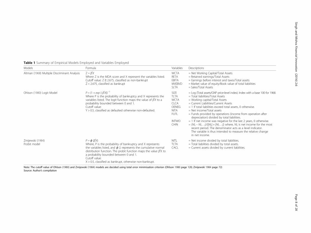
Table 1 Summary of Empirical Models Employed and Variables Employed
Models Formula Variables Descriptions
Altman (1968) Multiple Discriminant Analysis Z = βIXWhere Z is the MDA score and X represent the variables listed.Cutoff value: Z≥ 2.675, classified as non-bankruptZ < 2.675, classified as bankrupt
WCTARETAEBITAMVEBVDSLTA
= Net Working Capital/Total Assets= Retained earnings/Total Assets= Earnings before interest and taxes/Total assets= Market value of equity/Book value of total liabilities= Sales/Total Assets
Ohlson (1980) Logit Model P = (1 + exp {-βIX})−1
Where P is the probability of bankruptcy and X represents thevariables listed. The logit function maps the value of βIX to aprobability bounded between 0 and 1.Cutoff value:Y > 0.5, classified as defaulted otherwise non-defaulted.
SIZETLTAWCTACLCAOENEGNITAFUTL
INTWOCHIN
= Log (Total assets/GNP price-level index). Index with a base 100 for 1968.= Total liabilities/Total Assets= Working capital/Total Assets= Current Liabilities/Current Assets= 1 If total liabilities exceed total assets, 0 otherwise.= Net income/Total assets= Funds provided by operations (income from operation afterdepreciation) divided by total liabilities.
= 1 If net income was negative for the last 2 years, 0 otherwise.= (NIt − NIt − 1)/(|NIt| + |NIt − 1|) where, NIt is net income for the mostrecent period. The denominator acts as a level indicator.The variable is thus intended to measure the relative changein net income.
Zmijewski (1984)Probit model
P = ɸ (βIX)Where, P is the probability of bankruptcy and X representsthe variables listed, and ɸ (.) represents the cumulative normaldistribution function. The probit function maps the value βIX toa probability bounded between 0 and 1.Cutoff value:X > 0.5, classified as bankrupt, otherwise non-bankrupt.
NITLTLTACACL
= Net income divided by total liabilities.= Total liabilities divided by total assets.= Current assets divided by current liabilities.
Note: The cutoff value of Ohlson (1980) and Zmijewski (1984) models are decided using total error minimisation criterion (Ohlson 1980 page 120; Zmijewski 1984 page 72)Source: Author’s compilation
Singhand
Mishra
FinancialInnovation (2016) 2:6
Page8of
28

firm’s registered sick during 2006 to 2014. A set of matched non-distressed companies
are identified randomly on the basis of asset size and industry type. A total of 130 com-
panies comprising distressed and non-distressed companies are used for estimation
sample. A sample of 78 companies’ holdout for model validation. Financial information
of the companies is collected from their balance sheet and income statements. The Bal-
ance sheet and income statements of the companies at the end of each year are col-
lected from their respective websites. The estimated and holdout sample have been
classified into 14 industry category matching with their economic activity with the Na-
tional Industrial Classification Code (NIC) 3 digit classification of 2008 (See Table 2).
Selection of financial ratios
There is extensive literature on the use of financial ratios to predict bankruptcy of the
firms. Since Beaver (1966), various financial ratios were tried to foretell bankruptcy,
and they can be broadly classified into four categories, which measures firm’s leverage,
liquidity, profitability and turnover. Bellovary et al. (2007), in a survey paper on bank-
ruptcy prediction list 42 financial ratios which is used in more than five financial stud-
ies on bankruptcy prediction.
In the Indian market, Bandyopadhyay (2006) develops bankruptcy prediction model
based upon MDA and logistic technique for Indian corporate bond sector. The ratios
used in his study measures liquidity, leverage, productivity, turnover and other financial
variables which measures age, group ownership, ISO Quality Certification and inter-
industry effects of the firms. Bhumia and Sarkar (2011) in other study on Indian
pharmaceutical industry developed model for corporate failure using MDA technique.
The study chooses 16 financial ratios based upon past empirical literature measuring
Table 2 Distribution of Firms as per NIC Classification 2008
NICCode
Sector EstimationSample
HoldoutSample
Total
107 Manufacturer of other food products 14 6 20
131 Spinning, weaving and finishing of textiles 34 16 50
170 Manufacturer of paper and paper products 4 10 14
201 Manufacturer of basic chemicals, fertilizer and nitrogencompounds, plastics, synthetic rubber in primary form
18 6 24
210 Manufacturer of pharmaceuticals, medicinal chemicaland botanical products
6 2 8
221 Manufacturer of rubber products 4 4 8
231 Manufacturer of glass and glass products 4 2 6
239 Manufacturer of non-metallic mineral products n.e.c. 2 2
243 Casting of metals 16 6 22
261 Manufacturer of electronic components 6 16 22
271 Manufacturer of electric motors, generators, transformersand electricity distribution and control apparatus
4 4
291 Manufacturer of motor vehicles 8 6 14
310 Manufacturer of furniture 4 4
492 Other land transport 6 4 10
Total 130 78 208
Source: Author’s compilation
Singh and Mishra Financial Innovation (2016) 2:6 Page 9 of 28
profitability, solvency, liquidity and efficiency of the firms. Shetty et al. (2012) develops
early warning system for Indian IT/ITES using Data Envelopment Analysis (DEA).
Based upon the past empirical studies ten financial ratios measuring firm’s liquidity, le-
verage, productivity, and turnover. Kumar and Rao (2015) develops non-linear new Z-
score model based upon Person Type-3 distribution for Indian companies. In addition
to Altman (1968) variables, the study uses two other non-financial variables measuring
industry effects and rating of the companies. Based upon the past empirical literature
and our own analytical judgment, we have chosen 25 financial ratios measuring firm’s
leverage, liquidity, profitability, and turnover. In most of studies on global or Indian
market, they found leverage, liquidity, profitability and turnover are the major financial
ratio which predicts corporate failure.
Out of four major financial ratio leverage is considered to be one of the important ra-
tios to assess financial position of the firms. According to Argenti (1976) in his study,
he founds high indebtedness of the firms is one of the major reason leading a firm to
bankruptcy. Similarly, Jensen (1989) argues leverage is an invitation to bankruptcy, and
high debt ratios are not good for firms. In the Indian market Bandyopadhyay (2006),
Bhumia and Sarkar (2011), Shetty et al. (2012) and Kumar and Rao (2015) acknowl-
edges the importance of leverage ratio and uses different leverage indicators to assess
bankruptcy. Except Bhumia and Sarkar (2011) all other studies (Bandyopadhyay (2006),
Shetty et al. (2012) and Kumar and Rao (2015)) on Indian market have taken market
value of equity to book value of total debt as ratio measuring leverage of the firms. In
lieu of past empirical literature and importance of the indicators including market
value of equity to book value of total debt, 11 leverage ratios are chosen out of 25 fi-
nancial ratios.
Liquidity is also considered to be one of the important ratio to assess credit worthi-
ness of firms. Beaver (1966) in his study found the firms with lower liquid assets are
more prone to bankruptcy. In line with Beaver (1966), Altman, Haldeman and Nar-
ayana (1977), Charalambrus, Charitiu and Kaourou (2000) and Platt and Platt (2002)
also gets the similar findings. In the Indian market Bandyopadhyay (2006), Bhumia and
Sarkar (2011), Shetty et al. (2012) and Kumar and Rao (2015) all have used liquidity in-
dicator including working capital to total assets as a common liquidity indicator used
in all the four empirical studies. In the current study including working capital to total
assets, four liquidity indicators are used out of 25 financial ratios.
Profitability ratios measures the performance of the firms. The ratio explains how ef-
ficient and effective utilization of its assets and management of its expenditure to pro-
duce adequate earnings for its shareholders. According to Gu (2002), unprofitable firms
are more likely to default. Izan (1984), Maricca and Georgeta (2012) also got similar
findings in their respective studies. In the Indian context Bandyopadhyay (2006) uses
operating profits to total assets as the proxy for profitability indicator. Kumar and Rao
(2015) and Bhumia and Sarkar (2011) uses retained earnings to total assets as a proxy
for profitability indicator. In the current study out of 25 financial ratio, 7 profitability
ratios are chosen.
Turnover ratio measures efficiency of firms in utilizing their assets. Eljilly (2001) ar-
gues high efficiency leads to company profitable and less chance of bankruptcy and
vice-versa. It measures the ability of companies to generate sales by the capital invested.
Molinero and Ezzamel (1991) and Laitnen (1992) also founds the similar results. In the
Singh and Mishra Financial Innovation (2016) 2:6 Page 10 of 28

Indian market, Bandyopadhyay (2006) and Kumar and Rao (2015) have chosen Sales to
Total Assets as proxy for turnover ratio. In the present study including Sales to Total
Assets, 2 other turnover ratios are taken out of 25 ratios. The profile of variables used
in the study is reported in Table 3. To check industry specific effects, the sample firms
have been divided into 14 industry dummies based upon major economic activity as
per NIC classification (Table 5).
Following steps are followed to select final profile of the ratios:
Step-I: Analysis of Variables: We have chosen 25 financial ratios on the basis of past
empirical literatures on Indian market. Analyses on these ratios are carried out in two
broad steps. First, mean and standard deviation of bankrupt and non-bankrupt firms
are analysed. Second, T-test for equality in means of bankrupt and non-bankrupt
groups are analysed.
Table 3 Profile of Financial Ratios
Sl No. Financial Ratio Calculations
Leverage Ratios
1 TDTA Total Debt/Total Assets
2 BVEBVD Book Value of Equity/Book Value of Total Debt
3 CFOTA Cash Flow from Operations/Total Assets
4 CLTA Current Liabilities/Total Assets
5 CFTD Cash Flow from Operations/Total Debt
6 LTDTA Long-term Debt/Total Assets
7 NWTA Net Worth/Total Assets
8 TDNW Total Debt/Net Worth
9 TLNW Total Liabilities/Net Worth
10 TLTA Total Liabilities/Total Assets
11 FUTL Fund Provided by Operations to Total Liabilities
Liquidity
12 CACL Current Assets/Current Liabilities
13 WCTA Working Capital/Total Assets
14 CATA Current Assets/Total Assets
15 CLCA Current Liabilities/Current Assets
Profitability
16 NITA Net Income/Total Assets
17 RETA Retained Earnings/Total Assets
18 EBITA Earnings Before Interest and Taxes/Total Assets
19 NINW Net Income/Net Worth
20 CASL Current Assets/Sales
12 NISL Net Income/Sales
22 NITL Net Income/Total Liabilities
Turnover
23 SLTA Sales/Total Assets
24 WCSL Working Capital/Sales
25 WCNW Working Capital/Net Worth
Source: Author’s compilation
Singh and Mishra Financial Innovation (2016) 2:6 Page 11 of 28
Step-II: Step-wise regression: Forward logistic selection and backward elimination
methods are applied and different combinations of the ratios which are significantly
different in mean by T-test are tested and the final set of ratio are selected on the basis
of the statistical significance of the estimated parameters, the sign of each variable’s
coefficient and the model’s classification results.
Step-III: Inclusion of industry dummy: In the next step along with four financial ratios
14 industrial dummies were included in the model but none of them are found to be
significant. This is also tested trough through stepwise regression model. However, the
results are unchanged.
Step-IV: Final profile of the ratios: Finally, all the financial ratios which are found to
be statistically significant chosen for the model.
Analysis of variables
This sections covers analysis of mean and standard deviation of defaulted and non-
defaulted firms. T-test for equality in mean is employed to check weather defaulted,
and non-defaulted groups have significantly different in their respective means. It is
well-known from past empirical studies that the bankrupt companies have higher in-
debtedness, lower liquidity, poor profitability and turnover ratios. Also from Table 4,
out of three turnover ratios, WCSL mean is not found to be statistically different. For
defaulted groups it is found to be negative (WCSL and WCNW) and lower (SLTA) than
the defaulted groups. In case of profitability indicators, out of 7 financial ratios all
means are found to be significant expect CASL and NISL. For most of the profitability
indicators, the ratio is found to be negative (NITA, RETA, EBITA, and NITL) for
defaulted groups except NINW. For liquidity indicators out of 4, 2 turned to be statisti-
cally different means (WCTA, CLCA) and others are insignificant (CACL, CATA). In
case of leverage indicators, all indicators are statistically different in mean except CLTA.
For defaulted groups the ratios are found to be negative for all indicators except TDTA
and TLTA. From the analysis on variables, in general, most of ratios are grouped under
liquidity, profitability and turnover ratios have shown negative signs and declining for
bankrupt companies.
T-test for equality in means for defaulted and non-defaulted groups shows out of 25
financial ratios chosen for the model, 19 ratios have statistically different in mean be-
tween defaulted and non-defaulted groups.
Step-wise regression
In a step-wise regression, logistic forward selection and backward elimination methods
were applied and different combinations of the ratios (19 ratios) which had significantly
different in their respective means are tested. The selections of the final set of the vari-
ables are based upon statistical significance and sign of the each of the variable coeffi-
cients. The model classification power also took into consideration. The similar
method is also used by Neophytou et al. (2001) conducting study for Netherland firms.
The final set of ratios and their statistical significance is reported in third column
(Model 2) of Table 7. From Table 7 all the set of financial ratios are significant at 1 %
to 10 % level of significance, and LR ratio shows the overall significance of the model.
Singh and Mishra Financial Innovation (2016) 2:6 Page 12 of 28
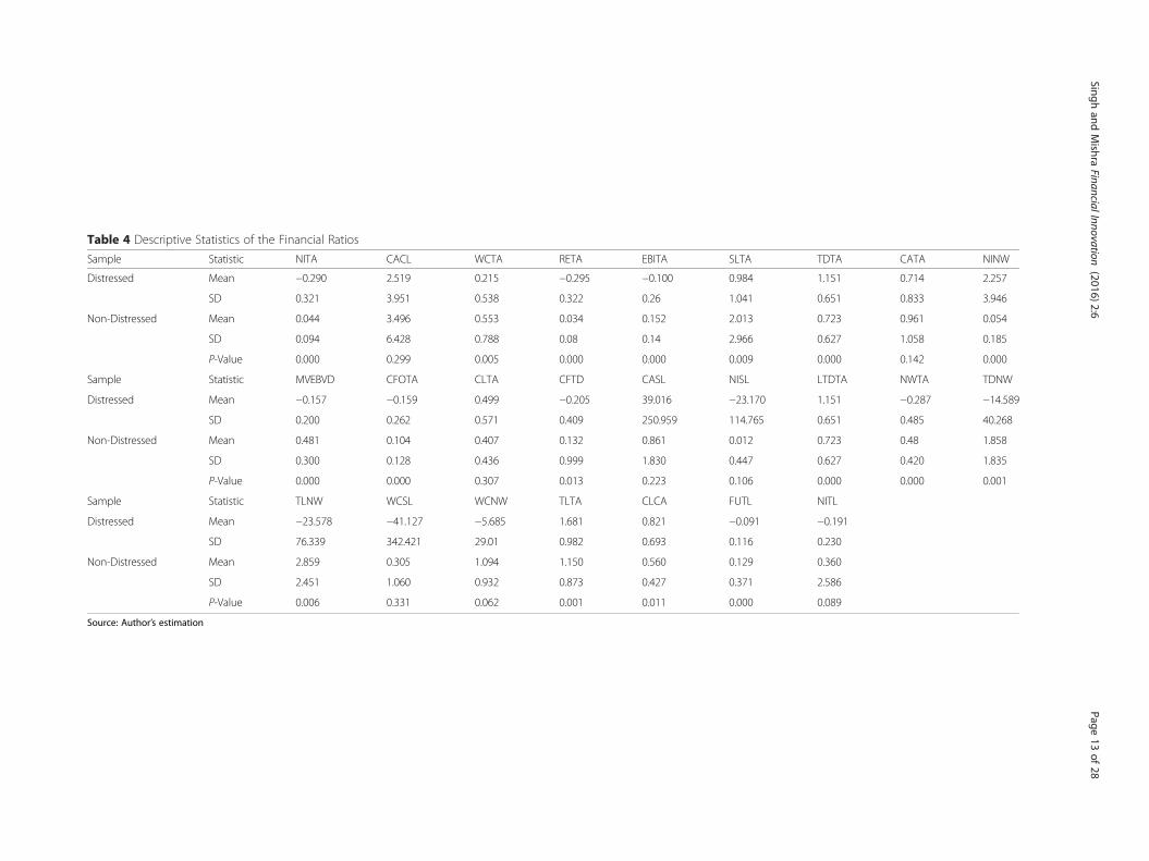
Table 4 Descriptive Statistics of the Financial Ratios
Sample Statistic NITA CACL WCTA RETA EBITA SLTA TDTA CATA NINW
Distressed Mean −0.290 2.519 0.215 −0.295 −0.100 0.984 1.151 0.714 2.257
SD 0.321 3.951 0.538 0.322 0.26 1.041 0.651 0.833 3.946
Non-Distressed Mean 0.044 3.496 0.553 0.034 0.152 2.013 0.723 0.961 0.054
SD 0.094 6.428 0.788 0.08 0.14 2.966 0.627 1.058 0.185
P-Value 0.000 0.299 0.005 0.000 0.000 0.009 0.000 0.142 0.000
Sample Statistic MVEBVD CFOTA CLTA CFTD CASL NISL LTDTA NWTA TDNW
Distressed Mean −0.157 −0.159 0.499 −0.205 39.016 −23.170 1.151 −0.287 −14.589
SD 0.200 0.262 0.571 0.409 250.959 114.765 0.651 0.485 40.268
Non-Distressed Mean 0.481 0.104 0.407 0.132 0.861 0.012 0.723 0.48 1.858
SD 0.300 0.128 0.436 0.999 1.830 0.447 0.627 0.420 1.835
P-Value 0.000 0.000 0.307 0.013 0.223 0.106 0.000 0.000 0.001
Sample Statistic TLNW WCSL WCNW TLTA CLCA FUTL NITL
Distressed Mean −23.578 −41.127 −5.685 1.681 0.821 −0.091 −0.191
SD 76.339 342.421 29.01 0.982 0.693 0.116 0.230
Non-Distressed Mean 2.859 0.305 1.094 1.150 0.560 0.129 0.360
SD 2.451 1.060 0.932 0.873 0.427 0.371 2.586
P-Value 0.006 0.331 0.062 0.001 0.011 0.000 0.089
Source: Author’s estimation
Singhand
Mishra
FinancialInnovation (2016) 2:6
Page13
of28
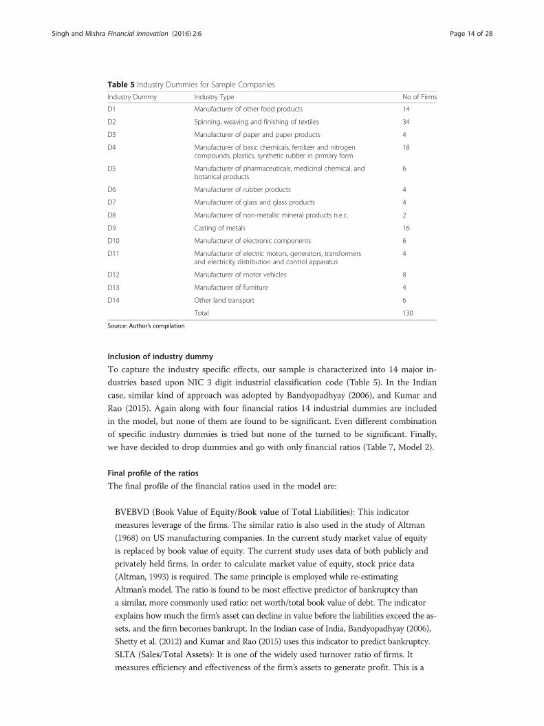
Inclusion of industry dummy
To capture the industry specific effects, our sample is characterized into 14 major in-
dustries based upon NIC 3 digit industrial classification code (Table 5). In the Indian
case, similar kind of approach was adopted by Bandyopadhyay (2006), and Kumar and
Rao (2015). Again along with four financial ratios 14 industrial dummies are included
in the model, but none of them are found to be significant. Even different combination
of specific industry dummies is tried but none of the turned to be significant. Finally,
we have decided to drop dummies and go with only financial ratios (Table 7, Model 2).
Final profile of the ratios
The final profile of the financial ratios used in the model are:
BVEBVD (Book Value of Equity/Book value of Total Liabilities): This indicator
measures leverage of the firms. The similar ratio is also used in the study of Altman
(1968) on US manufacturing companies. In the current study market value of equity
is replaced by book value of equity. The current study uses data of both publicly and
privately held firms. In order to calculate market value of equity, stock price data
(Altman, 1993) is required. The same principle is employed while re-estimating
Altman’s model. The ratio is found to be most effective predictor of bankruptcy than
a similar, more commonly used ratio: net worth/total book value of debt. The indicator
explains how much the firm’s asset can decline in value before the liabilities exceed the as-
sets, and the firm becomes bankrupt. In the Indian case of India, Bandyopadhyay (2006),
Shetty et al. (2012) and Kumar and Rao (2015) uses this indicator to predict bankruptcy.
SLTA (Sales/Total Assets): It is one of the widely used turnover ratio of firms. It
measures efficiency and effectiveness of the firm’s assets to generate profit. This is a
Table 5 Industry Dummies for Sample Companies
Industry Dummy Industry Type No of Firms
D1 Manufacturer of other food products 14
D2 Spinning, weaving and finishing of textiles 34
D3 Manufacturer of paper and paper products 4
D4 Manufacturer of basic chemicals, fertilizer and nitrogencompounds, plastics, synthetic rubber in primary form
18
D5 Manufacturer of pharmaceuticals, medicinal chemical, andbotanical products
6
D6 Manufacturer of rubber products 4
D7 Manufacturer of glass and glass products 4
D8 Manufacturer of non-metallic mineral products n.e.c. 2
D9 Casting of metals 16
D10 Manufacturer of electronic components 6
D11 Manufacturer of electric motors, generators, transformersand electricity distribution and control apparatus
4
D12 Manufacturer of motor vehicles 8
D13 Manufacturer of furniture 4
D14 Other land transport 6
Total 130
Source: Author’s compilation
Singh and Mishra Financial Innovation (2016) 2:6 Page 14 of 28
key variable for the measurement of the size of the firm. The capital-turnover ratio is
a standard financial ratio illustrating the sales generating ability of the firm’s assets. It
is one measure of management’s capability in dealing with competitive conditions. It is
used in the study of Altman (1968) and Bandyopadhyay (2006) and Kumar and Rao
(2015), used in the Indian market.
NITA (Net Income/Total Assets): It is the ratio of net income to total assets which is
a measure of performance of the firms. It measures profitability and also used in the
study of Ohlson (1980) on US manufacturing companies.
NITL (Net Income/Total Liabilities): It is the ratio of net income to total liabilities.
The ratio measures return on asset which is the measure of firm’s performance and
profitability. The ratio is also used in the study of Zmijewski (1984).
Broadly all the ratios used in the current study are from the studies of Altman
(1968), Ohlson (1980) and Zmijewski (1984). The first two ratio’s BVEBVD and SLTA
measuring leverage and turnover of the firms are also used in the Study of Altman
(1968). Third ratio NITA measures profitability of the firms is used in the study of Ohl-
son (1980), and fourth NITL measures profitability of firm is also applied in the study
of Zmijewski (1984). The new bankruptcy prediction model uses ratios measuring le-
verage, profitability, and turnover of the firms. The model is also considered to be com-
prehensive model because it uses variables from all three major accounting based
bankruptcy prediction model mentioned above. By ‘Common Sense’ and past studies all
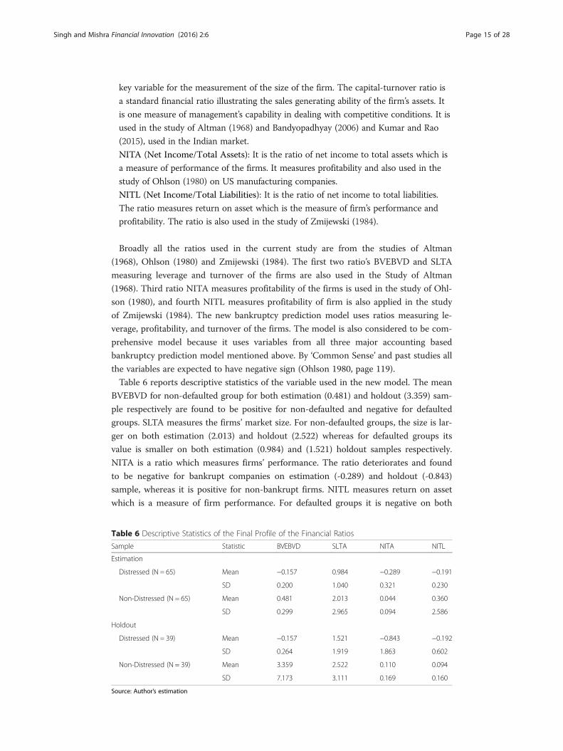
the variables are expected to have negative sign (Ohlson 1980, page 119).
Table 6 reports descriptive statistics of the variable used in the new model. The mean
BVEBVD for non-defaulted group for both estimation (0.481) and holdout (3.359) sam-
ple respectively are found to be positive for non-defaulted and negative for defaulted
groups. SLTA measures the firms’ market size. For non-defaulted groups, the size is lar-
ger on both estimation (2.013) and holdout (2.522) whereas for defaulted groups its
value is smaller on both estimation (0.984) and (1.521) holdout samples respectively.
NITA is a ratio which measures firms’ performance. The ratio deteriorates and found
to be negative for bankrupt companies on estimation (-0.289) and holdout (-0.843)
sample, whereas it is positive for non-bankrupt firms. NITL measures return on asset
which is a measure of firm performance. For defaulted groups it is negative on both
Table 6 Descriptive Statistics of the Final Profile of the Financial Ratios
Sample Statistic BVEBVD SLTA NITA NITL
Estimation
Distressed (N = 65) Mean −0.157 0.984 −0.289 −0.191
SD 0.200 1.040 0.321 0.230
Non-Distressed (N = 65) Mean 0.481 2.013 0.044 0.360
SD 0.299 2.965 0.094 2.586
Holdout
Distressed (N = 39) Mean −0.157 1.521 −0.843 −0.192
SD 0.264 1.919 1.863 0.602
Non-Distressed (N = 39) Mean 3.359 2.522 0.110 0.094
SD 7.173 3.111 0.169 0.160
Source: Author’s estimation
Singh and Mishra Financial Innovation (2016) 2:6 Page 15 of 28
estimation (-0.191) and holdout (-0.192) sample, whereas the ratio is found to be positive
for non-bankrupt firm on both estimation (0.360) and holdout (0.094) sample respectively.
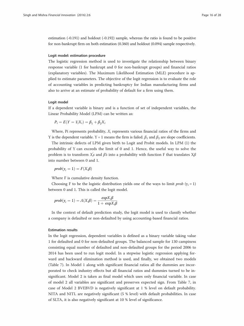
Logit model: estimation procedure
The logistic regression method is used to investigate the relationship between binary
response variable (1 for bankrupt and 0 for non-bankrupt groups) and financial ratios
(explanatory variables). The Maximum Likelihood Estimation (MLE) procedure is ap-
plied to estimate parameters. The objective of the logit regression is to evaluate the role
of accounting variables in predicting bankruptcy for Indian manufacturing firms and
also to arrive at an estimate of probability of default for a firm using them.
Logit model
If a dependent variable is binary and is a function of set of independent variables, the
Linear Probability Model (LPM) can be written as:
Pi ¼ E Y ¼ 1 Xij Þ ¼ β1 þ β2Xið
Where, Pi represents probability, Xi represents various financial ratios of the firms and
Y is the dependent variable. Y = 1 means the firm is failed. β1 and β2 are slope coefficients.
The intrinsic defects of LPM given birth to Logit and Probit models. In LPM (1) the
probability of Y can exceeds the limit of 0 and 1. Hence, the useful way to solve the
problem is to transform Xi’s and β’s into a probability with function F that translates Xβ
into number between 0 and 1.
prob yi ¼ 1ð Þ ¼ F Xiβð Þ
Where F is cumulative density function.
Choosing F to be the logistic distribution yields one of the ways to limit prob (yi = 1)
between 0 and 1. This is called the logit model.
prob yi ¼ 1ð Þ ¼ Λ Xiβð Þ ¼ expXiβ
1þ expXiβ
In the context of default prediction study, the logit model is used to classify whether
a company is defaulted or non-defaulted by using accounting-based financial ratios.
Estimation results
In the logit regression, dependent variables is defined as a binary variable taking value
1 for defaulted and 0 for non-defaulted groups. The balanced sample for 130 campiness
consisting equal number of defaulted and non-defaulted groups for the period 2006 to
2014 has been used to run logit model. In a stepwise logistic regression applying for-
ward and backward elimination method is used, and finally, we obtained two models
(Table 7). In Model 1 along with significant financial ratios all the dummies are incor-
porated to check industry effects but all financial ratios and dummies turned to be in-
significant. Model 2 is taken as final model which uses only financial variable. In case
of model 2 all variables are significant and preserves expected sign. From Table 7, in
case of Model 2 BVEBVD is negatively significant at 1 % level on default probability.
NITA and NITL are negatively significant (5 % level) with default probabilities. In case
of SLTA, it is also negatively significant at 10 % level of significance.
Singh and Mishra Financial Innovation (2016) 2:6 Page 16 of 28

LR ratio tests the overall significance of the model. In case of final model (Model 2)
the LR ratio is found to be 164.956 and statistically significant at 1 % level of signifi-
cance. The Model 2 can be directly used to find PDs of firms to assess credit risk.
Model re-estimations
This section covers re-estimation of Altman, Ohlson and Zmijewski models using esti-
mation sample of 130 Indian firms consisting equal numbers of defaulted and non-
defaulted firms. The statistical methodologies are the same used in the original models
and discussed in section 2. The stability of the coefficients of original models is tested
by comparing it from re-estimated models. The original and re-estimated coefficients
are reported in Table 11. The coefficients of original and re-estimated models are com-
pared to test the stability of coefficients to the time periods and change in the financial
conditions. The overall predictive accuracy of model is tested on estimation and holdout
sample to test whether change in coefficients (re-estimated) with recent data set improves
the predictive accuracy of the model. The newly proposed model is compared with ori-
ginal and re-estimated models. By overall predictive accuracy, ROC, long-range accuracy
test and the method to model bankruptcy, it is summarised that the newly proposed
model for Indian manufacturing sectors outperforms other competitive models.
Table 7 Results of Logit Model 1 and 2
Model 1 Model 2
Variables Coefficients Coefficients
MVEBVD −39.907 −13.8597a
SLTA −4.488 −1.11303c
NITA −72.776 −18.760b
NITL −107.685 −34.354b
C −7.012 −0.604
D1 13.256
D2 6.277
D3 −14.496
D4 Dropped
D5 −2.311
D6 8.592
D7 10.97
D8 Dropped
D9 3.865
D10 15.956
D11 Dropped
D12 −1.563
D13 Dropped
D14 7.767
LR Ratio 172.219 164.956
p-Value 0.000 0.000
Note: a, b and csignifies the level of significance at 1 %, 5 %, and 10 % respectively and LR is log likelihood ratioSource: Author’s estimation
Singh and Mishra Financial Innovation (2016) 2:6 Page 17 of 28
Descriptive statistics
Tables 8, 9 and 10 reports the descriptive statistics of the variables used in estimation
and holdout sample for Altman, Ohlson, and Zmijewski models respectively.
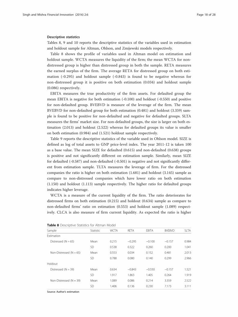
Table 8 shows the profile of variables used in Altman model on estimation and
holdout sample. WCTA measures the liquidity of the firm; the mean WCTA for non-
distressed group is higher than distressed group in both the sample. RETA measures
the earned surplus of the firm. The average RETA for distressed group on both esti-
mation (-0.295) and holdout sample (-0.843) is found to be negative whereas for
non-distressed group it is positive on both estimation (0.034) and holdout sample
(0.086) respectively.
EBITA measures the true productivity of the firm assets. For defaulted group the
mean EBITA is negative for both estimation (-0.100) and holdout (-0.550) and positive
for non-defaulted group. BVEBVD is measure of the leverage of the firm. The mean
BVEBVD for non-defaulted group for both estimation (0.481) and holdout (3.359) sam-
ple is found to be positive for non-defaulted and negative for defaulted groups. SLTA
measures the firms’ market size. For non-defaulted groups, the size is larger on both es-
timation (2.013) and holdout (2.522) whereas for defaulted groups its value is smaller
on both estimation (0.984) and (1.521) holdout sample respectively.
Table 9 reports the descriptive statistics of the variable used in Ohlson model. SIZE is
defined as log of total assets to GNP price-level index. The year 2011-12 is taken 100
as a base value. The mean SIZE for defaulted (0.615) and non-defaulted (0.638) groups
is positive and not significantly different on estimation sample. Similarly, mean SIZE
for defaulted (-0.587) and non-defaulted (-0.501) is negative and not significantly differ-
ent from estimation sample. TLTA measures the leverage of firm. For the distressed
companies the ratio is higher on both estimation (1.681) and holdout (3.145) sample as
compare to non-distressed companies which have lower ratio on both estimation
(1.150) and holdout (1.113) sample respectively. The higher ratio for defaulted groups
indicates higher leverage.
WCTA is a measure of the current liquidity of the firm. The ratio deteriorates for
distressed firms on both estimation (0.215) and holdout (0.634) sample as compare to
non-defaulted firms’ ratio on estimation (0.553) and holdout sample (1.089) respect-
ively. CLCA is also measure of firm current liquidity. As expected the ratio is higher
Table 8 Descriptive Statistics for Altman Model
Sample Statistic WCTA RETA EBITA BVEBVD SLTA
Estimation
Distressed (N = 65) Mean 0.215 −0.295 −0.100 −0.157 0.984
SD 0.538 0.322 0.260 0.200 1.041
Non-Distressed (N = 65) Mean 0.553 0.034 0.152 0.481 2.013
SD 0.788 0.080 0.140 0.299 2.966
Holdout
Distressed (N = 39) Mean 0.634 −0.843 −0.550 −0.157 1.521
SD 1.917 1.863 1.405 0.264 1.919
Non-Distressed (N = 39) Mean 1.089 0.086 0.214 3.359 2.522
SD 1.406 0.136 0.230 7.173 3.111
Source: Author’s estimation
Singh and Mishra Financial Innovation (2016) 2:6 Page 18 of 28
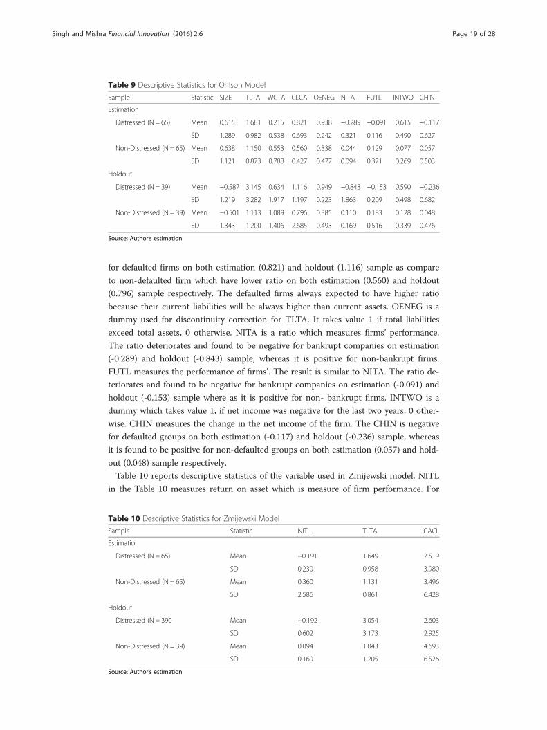
for defaulted firms on both estimation (0.821) and holdout (1.116) sample as compare
to non-defaulted firm which have lower ratio on both estimation (0.560) and holdout
(0.796) sample respectively. The defaulted firms always expected to have higher ratio
because their current liabilities will be always higher than current assets. OENEG is a
dummy used for discontinuity correction for TLTA. It takes value 1 if total liabilities
exceed total assets, 0 otherwise. NITA is a ratio which measures firms’ performance.
The ratio deteriorates and found to be negative for bankrupt companies on estimation
(-0.289) and holdout (-0.843) sample, whereas it is positive for non-bankrupt firms.
FUTL measures the performance of firms’. The result is similar to NITA. The ratio de-
teriorates and found to be negative for bankrupt companies on estimation (-0.091) and
holdout (-0.153) sample where as it is positive for non- bankrupt firms. INTWO is a
dummy which takes value 1, if net income was negative for the last two years, 0 other-
wise. CHIN measures the change in the net income of the firm. The CHIN is negative
for defaulted groups on both estimation (-0.117) and holdout (-0.236) sample, whereas
it is found to be positive for non-defaulted groups on both estimation (0.057) and hold-
out (0.048) sample respectively.
Table 10 reports descriptive statistics of the variable used in Zmijewski model. NITL
in the Table 10 measures return on asset which is measure of firm performance. For
Table 10 Descriptive Statistics for Zmijewski Model
Sample Statistic NITL TLTA CACL
Estimation
Distressed (N = 65) Mean −0.191 1.649 2.519
SD 0.230 0.958 3.980
Non-Distressed (N = 65) Mean 0.360 1.131 3.496
SD 2.586 0.861 6.428
Holdout
Distressed (N = 390 Mean −0.192 3.054 2.603
SD 0.602 3.173 2.925
Non-Distressed (N = 39) Mean 0.094 1.043 4.693
SD 0.160 1.205 6.526
Source: Author’s estimation
Table 9 Descriptive Statistics for Ohlson Model
Sample Statistic SIZE TLTA WCTA CLCA OENEG NITA FUTL INTWO CHIN
Estimation
Distressed (N = 65) Mean 0.615 1.681 0.215 0.821 0.938 −0.289 −0.091 0.615 −0.117
SD 1.289 0.982 0.538 0.693 0.242 0.321 0.116 0.490 0.627
Non-Distressed (N = 65) Mean 0.638 1.150 0.553 0.560 0.338 0.044 0.129 0.077 0.057
SD 1.121 0.873 0.788 0.427 0.477 0.094 0.371 0.269 0.503
Holdout
Distressed (N = 39) Mean −0.587 3.145 0.634 1.116 0.949 −0.843 −0.153 0.590 −0.236
SD 1.219 3.282 1.917 1.197 0.223 1.863 0.209 0.498 0.682
Non-Distressed (N = 39) Mean −0.501 1.113 1.089 0.796 0.385 0.110 0.183 0.128 0.048
SD 1.343 1.200 1.406 2.685 0.493 0.169 0.516 0.339 0.476
Source: Author’s estimation
Singh and Mishra Financial Innovation (2016) 2:6 Page 19 of 28
defaulted groups it is negative on both estimation (-0.191) and holdout (-0.192) sample,
whereas the ratio is found to be positive for non-bankrupt firm on both estimation
(0.360) and holdout (0.094) sample respectively. TLTA is the debt ratio which measures
the leverage of the firms. The distressed firms have higher leverage on both estimation
(1.649) and holdout sample (3.054) respectively. CACL measures the liquidity of the
firms. The non-distressed firm have higher liquidity ratio on both (3.496) and holdout
(4.693) sample as compared to distressed groups.
The profile analysis of the samples used in all the three models shows there is signifi-
cant difference in the mean ratios of the defaulted and non-defaulted groups. The ratios
deteriorates for bankrupt groups as compared to non-bankrupt groups.
Results and DiscussionThis section analyzed the findings of the original, re-estimated and newly proposed
models on estimation and holdout samples. The stability of their coefficients and their
predictive accuracies are also tested. This section also evaluates out of three models
which outperforms in the Indian setting.
Unstable coefficients
Table 11 reports the coefficients of original and re-estimated models. If the models are
stable, then their re-estimated coefficient should be also similar. The coefficients of ori-
ginal and re-estimated Altman model are reported in the Table 11.
The result shows there is significant difference in the coefficients of original and re-
estimated model except RETA. In case of RETA the original (1.4) and re-estimated
(1.464) coefficients is found to be very close. For WCTA original coefficient was 1.2,
and it ranks third with respect to relative importance of the variable to contribute in
the overall index. In the re-estimated model the coefficient (0.076) significantly changes
but still its ranks third in term of its relative importance in the overall index. In the ori-
ginal model EBITA, coefficient was 3.3, and it ranks first to contribute in the overall
index, whereas re-estimated coefficient (-.063) becomes negative and ranks fifth. In case
of BVEBVD, the original coefficient was 0.6 and re-estimated coefficient is 3.474 which
is significantly different. For SLTA, the original coefficient was 0.99 and re-estimated
coefficient is 0.028. The * indicates the statistical significance of F-statistic in the differ-
ence of mean. For both the Altman original and re-estimated models, the F-statistics is
significant, meaning that both the groups defaulted and non-defaulted have significantly
different means. The finding suggests the coefficients of Altman (1968) model are not
stable, and they are sensitive to time periods.
The results of Ohlson original and re-estimated models are also reported in Table 11.
In the original model, all the variables were significant except CLCA, INTWO and con-
stant whereas in the re-estimated model all the variables are significant except SIZE,
TLTA, FUTL and INTWO. The coefficients which are significant in both the original
and re-estimated models are WCTA, OENEG, NITA, and CHIN. In case of WCTA,
the original coefficient was -1.43 and re-estimated coefficient is -5.216 which is signifi-
cantly different. For OENEG the original coefficient was -1.72 and re-estimated coeffi-
cient is 2.836 which is different in value as well as in sign. There is huge difference in
the value of NITA coefficient for original (-2.37) and re-estimated (-29.676) model. In
Singh and Mishra Financial Innovation (2016) 2:6 Page 20 of 28
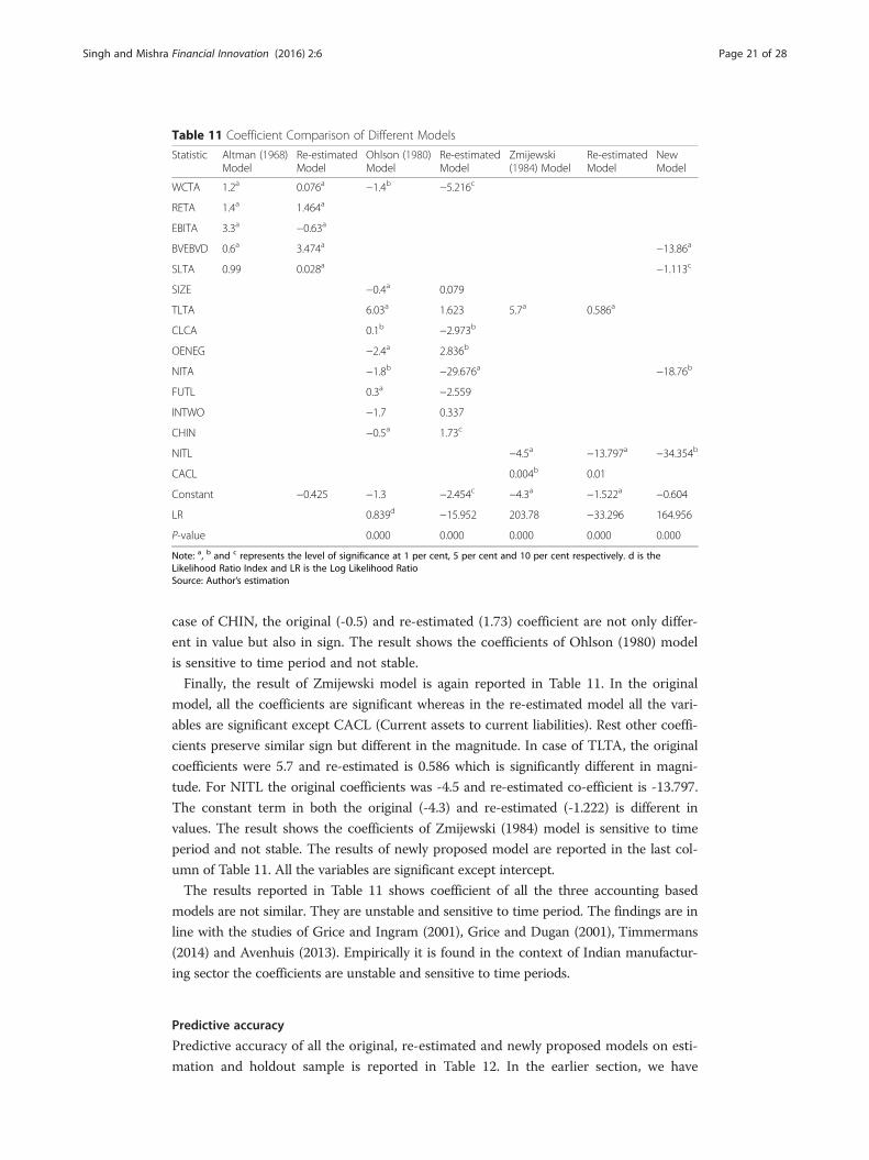
case of CHIN, the original (-0.5) and re-estimated (1.73) coefficient are not only differ-
ent in value but also in sign. The result shows the coefficients of Ohlson (1980) model
is sensitive to time period and not stable.
Finally, the result of Zmijewski model is again reported in Table 11. In the original
model, all the coefficients are significant whereas in the re-estimated model all the vari-
ables are significant except CACL (Current assets to current liabilities). Rest other coeffi-
cients preserve similar sign but different in the magnitude. In case of TLTA, the original
coefficients were 5.7 and re-estimated is 0.586 which is significantly different in magni-
tude. For NITL the original coefficients was -4.5 and re-estimated co-efficient is -13.797.
The constant term in both the original (-4.3) and re-estimated (-1.222) is different in
values. The result shows the coefficients of Zmijewski (1984) model is sensitive to time
period and not stable. The results of newly proposed model are reported in the last col-
umn of Table 11. All the variables are significant except intercept.
The results reported in Table 11 shows coefficient of all the three accounting based
models are not similar. They are unstable and sensitive to time period. The findings are in
line with the studies of Grice and Ingram (2001), Grice and Dugan (2001), Timmermans
(2014) and Avenhuis (2013). Empirically it is found in the context of Indian manufactur-
ing sector the coefficients are unstable and sensitive to time periods.
Predictive accuracy
Predictive accuracy of all the original, re-estimated and newly proposed models on esti-
mation and holdout sample is reported in Table 12. In the earlier section, we have
Table 11 Coefficient Comparison of Different Models
Statistic Altman (1968)Model
Re-estimatedModel
Ohlson (1980)Model
Re-estimatedModel
Zmijewski(1984) Model
Re-estimatedModel
NewModel
WCTA 1.2a 0.076a −1.4b −5.216c
RETA 1.4a 1.464a
EBITA 3.3a −0.63a
BVEBVD 0.6a 3.474a −13.86a
SLTA 0.99 0.028a −1.113c
SIZE −0.4a 0.079
TLTA 6.03a 1.623 5.7a 0.586a
CLCA 0.1b −2.973b
OENEG −2.4a 2.836b
NITA −1.8b −29.676a −18.76b
FUTL 0.3a −2.559
INTWO −1.7 0.337
CHIN −0.5a 1.73c
NITL −4.5a −13.797a −34.354b
CACL 0.004b 0.01
Constant −0.425 −1.3 −2.454c −4.3a −1.522a −0.604
LR 0.839d −15.952 203.78 −33.296 164.956
P-value 0.000 0.000 0.000 0.000 0.000
Note: a, b and c represents the level of significance at 1 per cent, 5 per cent and 10 per cent respectively. d is theLikelihood Ratio Index and LR is the Log Likelihood RatioSource: Author’s estimation
Singh and Mishra Financial Innovation (2016) 2:6 Page 21 of 28
mentioned based upon total error minimization principle, cut-off value is taken for all
the three models. The cut-off value for original Altman (1968), Ohlson (1980) and Zmi-
jewski (1984) models were 2.675, 0.5 and 0.5 respectively (Ohlson 1980 page 120; Zmi-
jewski 1984 page 72). In the re-estimated model based upon the same principle the
cut-off value for Altman, Ohlson and Zmijewski model is taken 0, 0.4 and 0.5 respect-
ively. For the newly proposed model same principle of total error minimization criter-
ion is followed and 0.6 is taken cut-off value for the model (Appendix 1, Table 14).
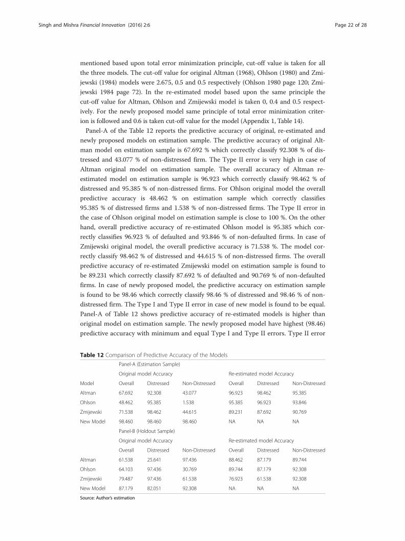
Panel-A of the Table 12 reports the predictive accuracy of original, re-estimated and
newly proposed models on estimation sample. The predictive accuracy of original Alt-
man model on estimation sample is 67.692 % which correctly classify 92.308 % of dis-
tressed and 43.077 % of non-distressed firm. The Type II error is very high in case of
Altman original model on estimation sample. The overall accuracy of Altman re-
estimated model on estimation sample is 96.923 which correctly classify 98.462 % of
distressed and 95.385 % of non-distressed firms. For Ohlson original model the overall
predictive accuracy is 48.462 % on estimation sample which correctly classifies
95.385 % of distressed firms and 1.538 % of non-distressed firms. The Type II error in
the case of Ohlson original model on estimation sample is close to 100 %. On the other
hand, overall predictive accuracy of re-estimated Ohlson model is 95.385 which cor-
rectly classifies 96.923 % of defaulted and 93.846 % of non-defaulted firms. In case of
Zmijewski original model, the overall predictive accuracy is 71.538 %. The model cor-
rectly classify 98.462 % of distressed and 44.615 % of non-distressed firms. The overall
predictive accuracy of re-estimated Zmijewski model on estimation sample is found to
be 89.231 which correctly classify 87.692 % of defaulted and 90.769 % of non-defaulted
firms. In case of newly proposed model, the predictive accuracy on estimation sample
is found to be 98.46 which correctly classify 98.46 % of distressed and 98.46 % of non-
distressed firm. The Type I and Type II error in case of new model is found to be equal.
Panel-A of Table 12 shows predictive accuracy of re-estimated models is higher than
original model on estimation sample. The newly proposed model have highest (98.46)
predictive accuracy with minimum and equal Type I and Type II errors. Type II error
Table 12 Comparison of Predictive Accuracy of the Models
Panel-A (Estimation Sample)
Original model Accuracy Re-estimated model Accuracy
Model Overall Distressed Non-Distressed Overall Distressed Non-Distressed
Altman 67.692 92.308 43.077 96.923 98.462 95.385
Ohlson 48.462 95.385 1.538 95.385 96.923 93.846
Zmijewski 71.538 98.462 44.615 89.231 87.692 90.769
New Model 98.460 98.460 98.460 NA NA NA
Panel-B (Holdout Sample)
Original model Accuracy Re-estimated model Accuracy
Overall Distressed Non-Distressed Overall Distressed Non-Distressed
Altman 61.538 25.641 97.436 88.462 87.179 89.744
Ohlson 64.103 97.436 30.769 89.744 87.179 92.308
Zmijewski 79.487 97.436 61.538 76.923 61.538 92.308
New Model 87.179 82.051 92.308 NA NA NA
Source: Author’s estimation
Singh and Mishra Financial Innovation (2016) 2:6 Page 22 of 28
is found to be more than 50 % in all the three original models. In case of original Ohlson
model, the Type II error is close to 100 %. All the three re-estimated models have higher
predictive accuracy and low Type I and Type II errors compared to original models.
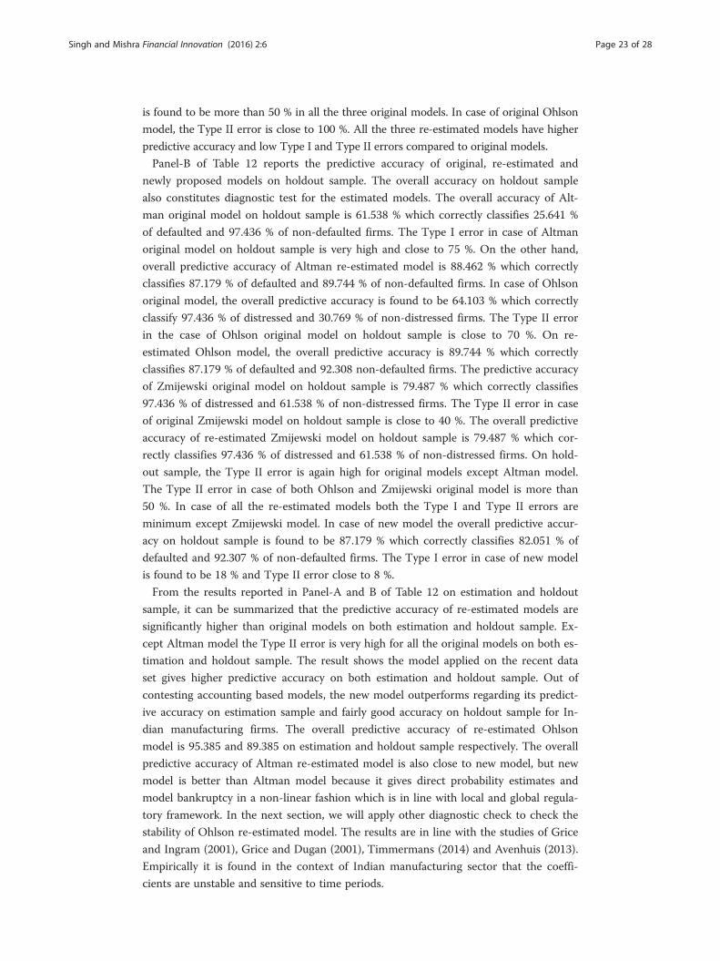
Panel-B of Table 12 reports the predictive accuracy of original, re-estimated and
newly proposed models on holdout sample. The overall accuracy on holdout sample
also constitutes diagnostic test for the estimated models. The overall accuracy of Alt-
man original model on holdout sample is 61.538 % which correctly classifies 25.641 %
of defaulted and 97.436 % of non-defaulted firms. The Type I error in case of Altman
original model on holdout sample is very high and close to 75 %. On the other hand,
overall predictive accuracy of Altman re-estimated model is 88.462 % which correctly
classifies 87.179 % of defaulted and 89.744 % of non-defaulted firms. In case of Ohlson
original model, the overall predictive accuracy is found to be 64.103 % which correctly
classify 97.436 % of distressed and 30.769 % of non-distressed firms. The Type II error
in the case of Ohlson original model on holdout sample is close to 70 %. On re-
estimated Ohlson model, the overall predictive accuracy is 89.744 % which correctly
classifies 87.179 % of defaulted and 92.308 non-defaulted firms. The predictive accuracy
of Zmijewski original model on holdout sample is 79.487 % which correctly classifies
97.436 % of distressed and 61.538 % of non-distressed firms. The Type II error in case
of original Zmijewski model on holdout sample is close to 40 %. The overall predictive
accuracy of re-estimated Zmijewski model on holdout sample is 79.487 % which cor-
rectly classifies 97.436 % of distressed and 61.538 % of non-distressed firms. On hold-
out sample, the Type II error is again high for original models except Altman model.
The Type II error in case of both Ohlson and Zmijewski original model is more than
50 %. In case of all the re-estimated models both the Type I and Type II errors are
minimum except Zmijewski model. In case of new model the overall predictive accur-
acy on holdout sample is found to be 87.179 % which correctly classifies 82.051 % of
defaulted and 92.307 % of non-defaulted firms. The Type I error in case of new model
is found to be 18 % and Type II error close to 8 %.
From the results reported in Panel-A and B of Table 12 on estimation and holdout
sample, it can be summarized that the predictive accuracy of re-estimated models are
significantly higher than original models on both estimation and holdout sample. Ex-
cept Altman model the Type II error is very high for all the original models on both es-
timation and holdout sample. The result shows the model applied on the recent data
set gives higher predictive accuracy on both estimation and holdout sample. Out of
contesting accounting based models, the new model outperforms regarding its predict-
ive accuracy on estimation sample and fairly good accuracy on holdout sample for In-
dian manufacturing firms. The overall predictive accuracy of re-estimated Ohlson
model is 95.385 and 89.385 on estimation and holdout sample respectively. The overall
predictive accuracy of Altman re-estimated model is also close to new model, but new
model is better than Altman model because it gives direct probability estimates and
model bankruptcy in a non-linear fashion which is in line with local and global regula-
tory framework. In the next section, we will apply other diagnostic check to check the
stability of Ohlson re-estimated model. The results are in line with the studies of Grice
and Ingram (2001), Grice and Dugan (2001), Timmermans (2014) and Avenhuis (2013).
Empirically it is found in the context of Indian manufacturing sector that the coeffi-
cients are unstable and sensitive to time periods.
Singh and Mishra Financial Innovation (2016) 2:6 Page 23 of 28
Diagnostics check for the New Model
This section deals with two diagnostics tests for newly proposed model, ROC and long-
range accuracy test.
The ROC (Hanley and McNeil, 1982) is one of the important and widely used test to
assess the performance of a binary classifier. The Area Under the Curve (AUC) sum-
marizes the performance of a model in a single number. The accuracy of the test de-
pends upon how well it classifies between the groups. In the present context, it is
between bankrupt and non-bankrupt. The model ROC with AUC 1 shows the perfect
test whereas the model with AUC 0.5 shows worthless test. As compare to a simple
metric of misclassification rate, ROC visualizes all possible classification thresholds.
In the ROC test the sensitivity or positive predictive value (PPV) is defined as the
proportion of firms for whom the outcome is positive that are correctly identified.
Similarly, the specificity or negative predictive value (NPV) is the probability that a firm
has a negative outcome given that they have a negative test result.
The ROC is the graph of specificity against 1-senstivity by which the impact of choice
is understood. A fairly excellent test have good balance between sensitivity and specifi-
city. The decision to set the classification threshold to predict out-of-sample data de-
pends upon the business decision.
Figure 1 shows the AUROC for re-estimated and new proposed model for bankruptcy
prediction. From the results, it is clear that new model shows the best results as com-
pare to other contesting models in application to the control. The AUROC for new
model is .985 which is higher than other contesting models. Hence, we can say this
model is the most appropriate model among contesting models for prediction of the
corporate failure for Indian manufacturing firms.
Table 13 reports the long-range accuracy results of new model on estimation and
hold-out sample. The long range accuracy of new model on estimation sample are
98.46 and 86.92 % for one year before bankruptcy and two years before bankruptcy re-
spectively. On the holdout sample, it is 89.74 and 70.51 % for one year and two years
before default respectively.
The long range accuracy results are fairly good and satisfactory. The result shows
the predictive accuracy of new model decreases as we go more backward from the
year of distress. Hence, the most recent information is helpful in predicting default
with higher accuracy.
ConclusionThe paper proposed a new model to predict the bankruptcy of Indian manufactur-
ing sector and also examines the sensitivity of Altman’s (1968), Ohlson’s (1980) and
Zmijewski’s (1984) models to the sample of 208 equal numbers of defaulted and
non-defaulted firms for the period 2006 to 2014 in the Indian context. The result
shows the overall accuracy of the model improves when the coefficients are re-
estimated. The overall accuracy of Altman (1968), Ohlson (1980) and Zmijewski
(1984) original models in the estimation sample are 67.692, 48.462 and 71.538 % re-
spectively. When all the models are re-estimated the accuracy improves to 96.923,
95.385 and 89.231 % respectively. On holdout sample, the overall accuracy of Alt-
man’s (1968), Ohlson’s (1980) and Zmijewski’s (1984) original models are 61.538,
64.103 and 79.487 % respectively. The accuracy improves to 88.462, 89.744 and
Singh and Mishra Financial Innovation (2016) 2:6 Page 24 of 28

76.923 when the models are re-estimated. The predictive accuracy of new model on
estimation and holdout sample is found to be 98.46 and 87.179 respectively. There-
fore, the new model is found to be a more robust model in comparison to Altman’s,
Ohlson’s and Zmijewski’s models. The major finding of the study suggests the coef-
ficients of the Altman’s (1968), Ohlson’s (1980) and Zmijewski’s (1984) models are
sensitive to time periods and financial condition. The predictive accuracy of the
models increases when more recent data are used in the estimation samples. The
change in the financial environment leads to change in the relation between finan-
cial distress and financial ratios. This also alters the comparative importance of the
ratios to predict default. Hence, researchers should re-estimate the original models
to get higher predictive accuracy. In case of Indian manufacturing companies, out
of all competitive accounting based models, the new model outperforms regarding
predictive accuracy, ROC, and long-range accuracy test.
The major limitation of the study is that it can be applied to only manufacturing
firms and excludes financial firms. The study can also use larger data set applying vari-
ous other parametric and non-parametric models to check validity of the model, ro-
bustness and stability of the parameters. Though, the results of Black-Scholes-Merton
(BSM) model can’t be directly compared with the proposed model but using Indian
manufacturing data the same approach can be applied to develop model for Indian
manufacturing companies.
Table 13 Long-range Accuracy of Newly Proposed Model
Years before distress Estimation sample Holdout Sample
1 98.460 89.743
2 86.923 70.513
Source: Author’s estimation
Fig. 1 Comparision of AUROC for re-estimated (Altman's Ohlson's and Zmijewski's) and new model
Singh and Mishra Financial Innovation (2016) 2:6 Page 25 of 28
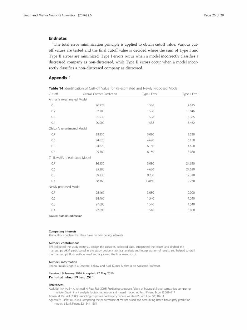
Endnotes1The total error minimization principle is applied to obtain cutoff value. Various cut-
off values are tested and the final cutoff value is decided where the sum of Type I and
Type II errors are minimized. Type I errors occur when a model incorrectly classifies a
distressed company as non-distressed, while Type II errors occur when a model incor-
rectly classifies a non-distressed company as distressed.
Appendix 1
Competing interestsThe authors declare that they have no competing interests.
Authors’ contributionsBPS collected the study material, design the concept, collected data, interpreted the results and drafted themanuscript. AKM participated in the study design, statistical analysis and interpretation of results and helped to draftthe manuscript. Both authors read and approved the final manuscript.
Authors’ informationBhanu Pratap Singh is a Doctoral Fellow and Alok Kumar Mishra is an Assistant Professor.
Received: 9 January 2016 Accepted: 27 May 2016
ReferencesAbdullah NA, Halim A, Ahmad H, Russ RM (2008) Predicting corporate failure of Malaysia’s listed companies: comparing
multiple Discriminant analysis, logistic regression and hazard model. Int Res J Financ Econ 15:201–217Adnan M, Dar AH (2006) Predicting corporate bankruptcy: where we stand? Corp Gov 6(1):18–33Agarwal V, Taffler RJ (2008) Comparing the performance of market-based and accounting based bankruptcy prediction
models. J Bank Financ 32:1541–1551
Table 14 Identification of Cutt-off Value for Re-estimated and Newly Proposed Model
Cut-off Overall Correct Prediction Type I Error Type II Error
Altman’s re-estimated Model
0 96.923 1.538 4.615
0.2 92.308 1.538 13.846
0.3 91.538 1.538 15.385
0.4 90.000 1.538 18.462
Ohlson’s re-estimated Model
0.7 93.850 3.080 9.230
0.6 94.620 4.620 6.150
0.5 94.620 6.150 4.620
0.4 95.380 6.150 3.080
Zmijewski’s re-estimated Model
0.7 86.150 3.080 24.620
0.6 85.380 4.620 24.620
0.5 89.230 9.230 12.310
0.4 88.460 13.850 9.230
Newly proposed Model
0.7 98.460 3.080 0.000
0.6 98.460 1.540 1.540
0.5 97.690 1.540 1.540
0.4 97.690 1.540 3.080
Source: Author’s estimation
Singh and Mishra Financial Innovation (2016) 2:6 Page 26 of 28

Altman EI (1968) Financial ratios, discriminant analysis and the prediction of corporate bankruptcy. J Financ 23(4):189–209Altman EI (1993) Corporate Financial Distress and Bankruptcy. John Wiley and Sons, Inc., New YorkAltman EI, Levallee MY (1980) Business Failure Classification in Canada. J Bus Adm 12(1):147–164Altman EI, Haldeman R, Narayanan P (1977) ZETA analysis, a new model for bankruptcy classification. J Bank Financ
1(1):29–54Altman EI, Marco G, Varetto F (1994) Corporate distress diagnosis: Comparisons using linear discriminant analysis and
neural networks (the Italian experience). J Bank Financ 18(3):505–529Argenti J (1976) Corporate Collapse: The Causes and Symptoms. McGraw-Hill, LondonAvenhuis JO (2013) Testing the generalizability of the bankruptcy prediction models of Altman,Ohlson and Zmijewski
for Dutch listed and large non-listed firms. Thesis submitted to School of Management and Governance. Universityof Twente, Netherlands
Balcaen S, Ooghe H (2004) 35 years of studies on business failure: an overview of the classical statistical methodologiesand their related problems. Working paper. Ghent University, June, 248: 1–62
Bandyopadhya A (2006) Predicting probability of default of Indian corporate bonds: logistic and Z-score modelapproaches. J Risk Financ 7(3):255–272
Beaver WH (1966) Financial ratios as predictors of failures. Journal of Accounting Research, Empirical Research inAccounting: Selected Studies 4:71–111
Begley J, Ming J, Watts S (1996) Bankruptcy classification errors in the 1980s: An empirical analysis of Altman’s andOhlson’s models. Rev Acc Stud 1:267–284
Bellovary J, Giacomino D, Akers M (2007) A review of bankruptcy prediction studies: 1930–present. J Financ Educ 33:1–42Bharath ST, Shumway T (2008) Forecasting default with the Merton distance to default model. Rev Financ Stud 21:1339–1369Bhunia A, Sarkar R (2011) A study of financial distress based on MDA. J Manag Res 3(2):1–11Black F, Cox J (1976) Valuing corporate securities: Some effects of bond indenture provisions. J Financ 31:352–367Black F, Scholes M (1973) The pricing of options and corporate liabilities. J Polit Econ 81(3):637–654Blum M (1974) Failing company discriminant analysis. J Account Res 12(1):1–25Boritz JE, Kennedy DB, Sun JY (2007) Predicting Business Failures in Canada. Account Perspect 6:141–165Charalambous C, Charitou A, Kaourou F (2000) Comparative analysis of artificial neural network models: Application in
bankruptcy prediction. Ann Oper Res 99:403–425Chudson W (1945) The Pattern of Corporate Financial Structure. National Bureau of Economic Research, New YorkCoats PK, Fant LF (1993) Recognizing financial distress patterns using a neural network tool. Financ Manag 22:142–155Deakin E (1972) A discriminant analysis of predictors of business failure. J Account Res 10(1):167–179Dimitras AI, Slowinski RS, Zoupounidis C (1999) Business failure prediction using rough sets. Eur J Oper Res 114(2):263–280Duffie D, Singleton K (1999) Modeling term structures of defaultable bonds. Rev Financ Stud 12:197–226Eljelly A, Mansour I (2001) Predicting private companies failure in the Sudan. J Afr Bus 2(2):23–43Etemadi H, Rostamy AAA, Dehkordi HF (2009) A genetic programming model for bankruptcy prediction: Empirical
evidence from Iran. Expert Syst Appl 36(2):3199–3207Fejér-Király G (2015) Bankruptcy Prediction: A Survey on Evolution, Critiques, and Solutions. Acta Universitatis
Sapientiae, Economics and Business 3(1):93–108FitzPatrick P (1932) A comparison of ratios of successful industrial enterprises with those of failed companies. The
Certified Public Accountant (October, November, December): 598-605, 656-662, and 727-731, respectivelyFulmer J, Moon J, Gavin T, Erwin M (1984) A bankruptcy classification model for small firms. Journal of Commercial
Bank Lending 66:25–37Georgeta V, Georgia TM (2012) Bankruptcy Prediction Model for Listed Companies in Romania. Journal of Eastern
Europe Research in Business & Economics Article ID 381337, DOI: 10.5171/2012.381337Grice JS, Dugan M (2001) The limitations of bankruptcy prediction models: Some cautions for the researcher. Rev
Quant Finan Acc 17:151–165Grice JS, Ingram RW (2001) Tests of the Generalizability of Altman’s Bankruptcy Prediction Model. J Bus Res 54(1):53–61Gu Z (2002) Analyzing bankruptcy in the restaurant industry: a multiple discriminant model. Int J Hosp Manag 21(1):25–42Guan Q (1993) Development of optimal network structures for back-propagationtrained neural networks. Ph.D.
dissertation. University of Nebraska, NebraskaGupta J, Gregoriou A, Healy J (2014) Forecasting bankruptcy for SMEs using hazard function: To what extent does size
matter? Rev Quant Finan Acc 2:1–25Hanley JA, McNeil BJ (1982) The meaning and use of the area under a Receiver Operating Characteristics curve.
Radiology 143:29–36Hillegeist S, Keating E, Cram D, Lundstedt K (2004) Assessing the probability of bankruptcy. Rev Acc Stud 9:5–34Izan H (1984) Corporate distress in Australia. J Bank Financ 8(2):303–320Jackendoff N (1962) A Study of Published Industry Financial and Operating Ratios. Temple University, Bureau of
Economic and Business Research, PhiladelphiaJarrow R, Turnbull S (1995) Pricing derivatives on financial securities subject to credit risk. J Financ 50:53–85Jensen MC (1989) Active Investors, LBOs and the Privatization of Bankruptcy. Journal of Applied Corporate Finance 2(1): 35–44.Kirkos E (2015) Assessing methodologies for intelligent bankruptcy prediction. Artif Intell Rev 43:83–123Koro T, Korodi A (2011) An evaluation of effectiveness of Fuzzy logic model in predicting the business bankruptcy.
Romanian Journal of Economic Forecasting 3:92–107Kulkarni A, Mishra AK, Thakker J (2005) How Good is Merton Model at Assessing Credit Risk? Evidence from India.
National Institute of Bank ManagementKumar MN, Rao VSH (2015) A New Methodology for Estimating Internal Credit Risk and Bankruptcy Prediction under
Basel II Regime. Comput Econ 46(1):83–102Laitinen EK (1992) Prediction of failure of a newly founded firm. J Bus Ventur 7(4):323–340Lando D (1994) Three essays on contingent claims pricing. Ph.D. dissertation. Cornell UniversityLee S, Choi WS (2013) A multi-industry bankruptcy prediction model using back-propagation neural network and
multivariate discriminant analysis. Expert System with Applications 40:2941–2946
Singh and Mishra Financial Innovation (2016) 2:6 Page 27 of 28
Lee KC, Han I, Kwon Y (1996) Hybrid neural network models for bankruptcy predictions. Decis Support Syst 18(1):63–72Legault J, Veronneau P (1986) CA-Score, Un Modele De Prevision De Faillite. ResearchReportLeland H, Toft K (1996) Optimal capital structure, endogenous bankruptcy, and the term structure of credit spread. J
Financ 51:987–1019Lonfstaff F, Schwartz E (1995) A simple approach to valuing risky fixed and floating rate debt. J Financ 50:789–819Merton R (1974) On the pricing of corporate debt: The risk structure of interest rates. J Financ 29:449–470Merwin C (1942) Financing small corporations in five manufacturing industries, 19261936. National Bureau of Economic
Research, New YorkMessier W Jr, Hansen J (1988) Inducing rules for expert system development: an example using default and bankruptcy
data. Manag Science 34(12):1403–1415Molinero M, Ezzamel M (1991) Multidimensional Scaling Applied to Corporate Failure. Omega Int J Manag Sci 19(4):259–274Neophytou E, Charitou A, Charalambous C (2001) Predicting corporate failure: Empirical evidence for the UK. Discussion
Paper No. 01-173, March, School of Management. University of Southampton, SouthamptonOhlson JA (1980) Financial ratios and the probabilistic prediction of bankruptcy. J Account Res 18(1):109–131Platt DH, Platt MB (1990) Development of a class of stable predictive variables: The case of bankruptcy prediction. J Bus
Financ Account 17:31–5Platt HD, Platt MB (2002) Predicting corporate financial distress: reflections on choice-based sample bias. J Econ Financ
26(2):184–199Pongsatat S, Ramage J, Lawrence H (2004) Bankruptcy prediction for large and small firms in Asia: a comparison of
Ohlson and Altman. J Account Croporate Governance 1(2):1–13Premachandra IM, Bhbra GS, Sueyoshi T (2009) DEA as a tool for bankruptcy assessment: A comparative study with
logistic regression technique. Eur J Oper Res 193:412–424Raghupathi W, Schkade LL, Raju BS (1991) A neural network application for bankruptcy prediction. In System Sciences,
1991. Proceedings of the Twenty-Fourth Annual Hawaii International Conference IEEE 4:147–155Ramakrishnan PR (2005) Financial Distress Prediction Models: A Case of Potential Sick Companies in India. The ICFAI
Journal of applied Finance 68-77. http://www.iupindia.in/1005/IJAF_Financial_Distress_68.htmlShetty U, Pakkala TPM, Mallikarjunappa T (2012) A modified directional distance formulation of DEA to assess
bankruptcy: An application to IT/ITES companies in India. Expert Systems with Applications 39(2):1988–1997Smith R, Winakor A (1935) Changes in Financial Structure of Unsuccessful Industrial Corporations. Bureau of Business
Research, Bulletin No. 51. University of Illinois Press, UrbanaSpringate GLV (1978) Predicting the Possibility of Failure in a Canadian Firm. Unpublished M.B.A. Research Project,
Simon Fraser UniversityTimmermans M (2014) US Corporate Bankruptcy Prediction Models: How accurate are the bankruptcy predicting
models of Altman (1968), Ohlson (1980) and Zmijewski (1984) after recalibration, when they are applied to U.S.listed firms in the period after the BACPA change in bankruptcy law? Thesis submitted to Tilburg University Schoolof Economics and Management. ANR: 876937
Tsukuda J, Baba SI (1994) Predicting Japanese corporate bankruptcy in terms of financial data using neural network.Comput Ind Eng 27(1):445–448
Ugurlu M, Aksoy H (2006) Prediction of corporate financial distress in an emerging market: the case of Turkey: CrossCultural Management. Int J 13(4):277–295
Vareto F (1998) Genetic algorithms applications in the analysis of insolvency risk. J Bank Financ 22:1421–1439Varma JR, Raghunathan V (2000) Modeling credit risk in Indian bond markets. ICFAI Journal of Applied Finance 6(3):53–67Verikas A, Kalsyte Z, Bacauskiene M, Gelzinis A (2010) Hybrid and ensemble-based soft computing techniques in
bankruptcy prediction: a survey. Soft Comput 14:995–1010Wu Y, Gaunt C, Gray S (2010) A comparison of alternative bankruptcy prediction models. J Contemp Account Econ 6:35–45Zmijewski ME (1984) Methodological issues related to the estimation of financial distress prediction models. J Account
Res 22:59–82
Submit your manuscript to a journal and benefi t from:
7 Convenient online submission
7 Rigorous peer review
7 Immediate publication on acceptance
7 Open access: articles freely available online
7 High visibility within the fi eld
7 Retaining the copyright to your article
Submit your next manuscript at 7 springeropen.com
Singh and Mishra Financial Innovation (2016) 2:6 Page 28 of 28