$ $ $ $ $ $ $ $ $ $ $ $ $ $ $ $ $ $ $ $ $ $ $ $ $ $ $ $ $ $ $ $ $ $ $ $ $ $ $ $ $ $ $ $

Miguel Bachrach and William J. Vaughan

Household Water DemandEstimation

S ) ) ) ) ) ) ) ) ) ) ) ) ) ) Q

Working Paper ENP106

Inter-American Development BankProductive Sectors and Environment SubdepartmentEnvironment Protection Division

March 1994

$ $ $ $ $ $ $ $ $ $ $ $ $ $ $ $ $ $ $ $ $ $ $ $ $ $ $ $ $ $ $ $ $ $ $ $ $ $ $ $ $ $ $

Household Water Demand Estimation

Miguel Bachrach and William J. Vaughan

March 1994

Miguel Bachrach, formerly an Operations Evaluation Officer at the Inter-American Development Bank, is now in private business. William J. Vaughanis a Senior Economist in the Project Analysis Department of the IDB.

This paper was originally developed for the IDB's Operations Evaluation Officeas background for the ex-post evaluation of rural potable water projects. Theauthors thank Jorge Ducci, Christian Gómez, and Glenn Westley for theircomments and suggestions. The views and opinions expressed herein arethose of the authors and do not represent the official position of the Inter-American Development Bank. This paper has undergone an informal reviewprocess but has not been submitted to a formal peer review. Its purpose is toelicit reader comments and suggestions, and is primarily intended for internaluse. Comments should be forwarded directly to the authors.

Inter-American Development Bank1300 New York Avenue, N.W.

Washington, D.C. 20577

- 4 -

Household Water Demand Estimation

C O N T E N T S

General Demand Estimation Issues

Simultaneity, Alternative Price Measures, and Multiple Equilibria

SimultaneityChoice of VariablesProperties of the Demand Function

Sample Selection Bias

Problems with Ordinary Least Squares, even in the Absence of SimultaneityThe Heckman Approach: Sample Selection Bias Correction with no SimultaneousEquationsExtension of the Sample Selection Model to the Simultaneous Equations Situation

Model Specifications and Data

Supply VariablesDemand VariablesWater Demand Equation Specification

Estimation Results

Conclusions

Simultaneous Equation Bias ExistsAverage Price May not be RelevantSample Selection Bias May MatterWhat to Do?

References

Another issue is whether the presence of declining block rates invalidates the estimation of individual1

demand curves because of the possibility of multiple equilibria. With micro data on individuals facingdecreasing block rate tariffs, a continuous, unique demand schedule may not exist.

In the application to rural localities in Argentina (see below), estimation with this data is complicated2

by the fact that a large number of customers fall in the fixed charge, minimum consumption block. Itwould not be uncommon to expect this in localities serving relatively poor households having few

Household Water Demand Estimation

To estimate the benefits of a potable water supply project, some idea of the parameters ofthe demand function is needed to calculate a Marshallian consumer's surplus welfare measure.Often, given a baseline estimate of pre-project consumption and price, an elasticity estimatecan be used to reconstitute the underlying demand function and the consumer surplus integral(see Powers and Valencia 1980), but the elasticity has to be obtained from the econometricestimation of a demand relation. In an early review of twenty-six household water demandelasticity estimates published before 1978, Hanke (1978) reported a wide range, the lowestestimate being -0.01 and the highest -6.71. Gómez (1987) reports a narrower range from theBank's own work in Latin America and the Caribbean, with all estimates below -0.65.

Any estimate of the benefits of a reduction in the price of water due to a water supply projectarrived at using an elasticity-based calculation will be sensitive to the magnitude of thatelasticity. So will the benefits based on a method that uses estimated demand functionsdirectly. This paper discusses the relative merits of the statistical procedures that can beused to obtain elasticity estimates or their underlying water demand functions.

General Demand Estimation Issues

A review of the water demand literature indicates that most problems encountered in demandestimation and the techniques available to address them are derived from or have been dealtwith in the literature on electricity demand. In both cases, the issues discussed mostfrequently have been:

1) Whether there is a simultaneous equations problem when estimating demand for waterwith multipart rate schedules and, if there is one, what techniques should be used tocorrect for it?

2) Whether average or marginal price is the relevant measure in estimating the demandfunction.1

In addition to these problems, another issue that has historically not received as muchattention in the water demand literature is how to deal with sample selection bias in the faceof a rate schedule combining a fixed charge for consumption below the level where a blockrate tariff per unit consumed takes effect. Accounting for this phenomenon in statisticalestimation, possibly in combination with (1) and (2) above, essentially involves deciding howto handle observations in the fixed charge category, where no unit consumption price isobserved. 2

- 2 -

expensive water-using appliances. If marginal price for this group is arbitrarily set to zero in estimationthe slope of the demand curve will be biased. Removing these observations from the estimation sampleintroduces sample selection bias.

The following two sections review each of these problems. The next section explains thedata setup, after which the results of estimating water demand functions using a sample of685 families from 34 localities in rural Argentina taken in 1987 are presented and discussed.The results obtained with the different estimation techniques designed to address the issuesidentified above are compared, and some conclusions are drawn in a final section.

Simultaneity, Alternative Price Measures, and Multiple Equilibria

Simultaneity

Until recently, the water demand literature has paid limited attention to simultaneity problems.It is worthwhile discussing this in some detail since the presence of, and the differentsolutions to, simultaneity have direct implications for the method of demand estimation.

A necessary condition for unbiased and consistent parameter estimation under Ordinary LeastSquares (OLS) is that there be no correlation between the error term and any of theexplanatory variables. With multipart block rates this condition is not fulfilled, since prices areendogenously determined by the consumer along with quantity demanded. Even though therate schedule (the supply function) is knowable a-priori by the investigator, the consumerchooses the preferred price-quantity pair, implying that both price and quantity areendogenous, not just quantity subject to a fixed price. Or, said otherwise, unless price isinfinitely elastic, a simultaneous equations problem theoretically must exist in the face ofblock rate schedules even if the parameters of the latter are known a-priori (Westley 1984).To illustrate this problem let us start with a simple demand function of the form:

Q = " + $ *Y + $ *P + u (1)1 2

where: Q = quantity demanded ",$ = parametersY = incomeP = priceu = random error term

If we were estimating the demand for domestic appliances by individual households, forexample, it is unlikely that purchases made by any household would affect the market price.At this micro level, market prices are not influenced by (are independent of) the quantitydemanded by a single household, so the error term (u) in Eq. (1) is uncorrelated with P.

In contrast, the price of water chosen by any household will be correlated with the randomerror term in Eq. (1) if the supplier's water tariff schedule relates the price charged to thequantity a household purchases.

- 3 -

This is an intuitively appealing assumption. The paradigm of the ideal consumer who is fully aware of3

all the rates in the water tariff schedule and exhibits optimizing behavior by equating marginalwillingness to pay to marginal supply price in a particular block ignores the cost of acquiring informationabout tariff rates for a commodity that usually commands a small share of total household expenditure. Although the approximating behavior embodied in the concept of average rather than marginal pricemakes intuitive sense, it cannot be accepted with our Argentinean data set (see the Results section). The water demand literature has debated this issue at length. For a recent and particularly goodexplanation, see Nieswiadomy and Molina (1991).

Suppose the relevant price for the consumer is the average price of water, and the price3

depends in stepwise block fashion on the amount consumed:

P̄ = [(P + r (q - q ) + r (q - q ) + ......+ r (Q - q ))]/Q (2)f 1 1 f i i+1 i j j-1

where:

q = quantity available for consumption at a fixed chargefP = fixed charge for water consumption at or below qf fr = block rate for block i (where j is the last consmption block)iq = block interval for block i.iP̄ = average priceQ = total quantity consumed.

By substituting Eq. (1) in Eq. (2) it is easy to see how the errors from Eq. (1) are correlatedwith P. With three blocks, Eq. (2) can be written as:

P + r (q -q ) + r (q -q ) - r q (3)f 1 1 f 2 2 1 3 2P̄ = ----------------------------------------- + r 3ó Q ûSubstituting the expression for Q from Eq.(1) in the denominator of (3) we have:

P + r (q -q ) + r (q -q ) - r q (4)f 1 1 f 2 2 1 3 2P̄ = ----------------------------------------- + r3ó " + $ *Y + $ *P + u û0 1 2

The error term (u) in the denominator of Eq. (4) is correlated with the average price, so biasin all parameter estimates of $ will be introduced if P̄ is used as an independent variable toiestimate Eq. (1). The larger the error term (u) the smaller the average price, since theconsumption level will be in one of the blocks with lower marginal rates.

D0

D1

P0

Q1 Q0 Q2

Quantity

Price D0

D1

Error

Error

Random

Random

- 4 -

For an exception, see Nieswiadomy and Molina (1991) who reject the OLS assumption of price4

exogeniety using the Hausman test.

A review of water demand analyses performed for IDB projects shows that OLS rather than IV5

estimation has always been used. Chicone and Ramamurthy (1986) make an argument for OLS basedon the evidence from previous studies.

Figure 1. Error and Price Correlation.

Even if the quantity demanded is a functionof the marginal price of water instead of theaverage price, the same simultaneity biasproblem can exist. In Figure 1 the real (andunobserved) household demand schedule D0intersects the supply schedule in the blockwhere the price is P0. With incomeconstant, suppose an exogenous randomevent like a change in weather causes achange in the quantity demanded. Arandom increase in water consumptionwould be observed as, say, Q2 and arandom decrease would be observed as Q1.The error term (u) is negatively correlatedwith price (P), since a large and positiverandom error (u) reduces the observed P anda large negative error increases the observedP. The OLS assumption of independencebetween the error term and the explanatoryvariables is violated because the water priceis not a constant--it depends on the quantitychosen. As a consequence OLS estimationwill erroneously yield the parameters of D1instead of D0. In other words, using OLSwith a declining block schedule willunderestimate or overestimate demandelasticity depending on whether the supply schedule is steeper than the demand schedule.With a rising block schedule the price response would be overestimated.

In the face of simultaneity, instrumental variables (IV) estimators such as two stage leastsquares (2SLS) are preferable to ordinary least squares to produce consistent parameterestimates. Curiously there is no consensus in the water demand literature on this issue.While the presence of simultaneous equation bias and the need for instrumental variablesestimation could be resolved via a Hausman test on a case by case basis (Hausman 1978,Nakamura and Nakamura 1981) empirical tests for simultaneity bias are uncommon in thewater demand literature. The use of OLS has often been justified a-priori on the basis of4

intuition, custom, or (to us) apparently specious reasoning, without bothering to test for thevalidity of the OLS error assumptions.5

Another way to understand demand function identification is illustrated in Figure 2. There thethree demand schedules represent the demand of three families with identical characteristicsexcept for income (which rises from D0 to D2). The decreasing block rate supply schedule

Quantity

Price

D0

D1

D2

- 5 -

This assumes that the price slope of the demand function is constant over time or across localities,6

respectively. Otherwise the demand function cannot be identified.

Having sufficient variation may be more complicated than it seems. In our sample we had some7

multicollinearity problems when constructing representations of the rate schedule using Westley'smethod.

Figure 2. Demand Not Identified

represents the tariff regime in the locality (S ). With this information it is not possible to0identify the demand function since the only data available are the three points of intersectionbetween the three separate demand schedules and the three block rates representing thesegments of the single public utility rate (supply) schedule. With the information in Figure 2,OLS can only produce a linear approximation of the discontinuous step function for supply;the parameters of the demand function are not identifiable.

In order to distinguish supply from demand we need some variation in the supply schedule thatcan be accounted for by an independent variable that does not affect the demand schedule.This condition is usually obtained by usingmore than one rate schedule (as in Figure 3).These can be constructed using time seriesinformation on rates for a single community,a cross-section of different communities, orboth.

An identifiable demand function is depictedin Figure 3. The several supply schedules S0to S clearly trace out the several demand2schedules. 6

The problem of simultaneity in the presenceof a block rate structure has been dealt within three ways. The first solution is to applytwo-stage least squares, as in Halvorsen(1975) or Westley (1984). For example, ina system like:

Q = " + $ *Y + $ *P + u (5)1 2

P = f(R(l,t),Q) (6)

where: R = rate schedulel = localityt = time

one can estimate the structural coefficients of (5) by regressing marginal price, P, against allthe independent variables of the system, and then using the prediction of P (P) in equation (5).^An important requirement for the applicability of this method is to have a known set of rateschedules with sufficient variation either in time period or by locality.7

Quantity

Price

D0

D1

D2

S2

S1

S0

S2

S1

S0S2S1

S0

- 6 -

A technical presentation of the properties of this technique may be found in Dutta (1975).8

The weights in each interval given by the number of people in the locality that consume in that9

particular interval with respect to the total number of people in the interval for the whole state.

Each interval can be defined at the lower level to avoid indeterminacy of the last block.10

Figure 3. Identified Demand

The second way to solve the simultaneity problem is byapplying fixed point or iterative least squares methods(see Martin et.al., 1984). These techniques are similar to2SLS, and basically consist of estimating (5) and (6)independently and using the predicted values of Q and P(Q and P) to reestimate (5) and (6) in a second iteration.^ ^This process is repeated until the values of Q and P^ ^converge. This technique was not applied to our survey8

because its statistical properties are less well known than2SLS.

The third solution actually argues that there is no realsimultaneity if the problem is properly specified(Blattenberger 1977, and Taylor, Blattenberger andRennhack 1981 and 1982). It is argued that demand andsupply relations can be derived and estimated from areduced form. In this formulation the consumer makes adecision based on the entire rate schedule; viz:

Q = " + $ *Y + $ *[R(l,t)] + u (7)0 1

The schedule R(l,t) is exogenous to the amount purchased, and in a formulation like Eq. (7)there is no apparent simultaneity problem. While the rate schedule can be represented inmany ways to estimate (7), its economic meaning is not entirely clear. Moreover, mostproxies that could represent the rate schedule will be correlated with the amount of waterconsumed. In particular, the two proxies normally chosen are the average price of water(Pavg) or the marginal price of water (Pmarg), which will be correlated to the quantity ofwater consumed. A solution to this problem is to create an artificial approximation to the rateschedule and derive average or marginal prices from it. Two approximations proposed byTaylor, Blattenberger and Rennhack 1981 (TBR) in the case of electricity can be directlyapplied to water demand estimation.

The first creates a linear approximation to the electricity bill (B ) and derives marginal pricesifrom it. In the case of TBR, who work with aggregate data, the first step was to take theelectricity bill in each locality at discrete consumption intervals and aggregate each intervalby state. For example, if the first interval is from 0 to 100 Kwh/month, and there are 509

localities in each state, the first observation, B( ), would represent the weighted average total1cost of water in the 100 Kwh/month interval for the 50 localities. Assuming there are Kdifferent intervals, the second step is to regress the B "observations" against consumption,kor rather, against each particular interval limit (Q ). That is, if B( ) is the average bill for ak k

10

particular block they regress:

Other

Goods

Water

Q0Q1

O0

O1

[O]

- 7 -

The significance of intramarginal cost will be explained below.11

Of TBR's two instruments, in our empirical application we found the rate schedule approximation was12

more satisfactory, but used neither in our final runs. See Section E for a discussion of the alternative

Figure 4. Marginal Rate Change.

B( ) = " + $*Q + u (8)k k

From (8) the estimate of $ is interpreted as the marginal price, while the intercept " isinterpreted as the intramarginal cost. Applying this method to the sample of rural11

communities in Argentina we linearized the rate schedule of each locality around discreteblocks common to all localities in the sample (from 1 to 65 m /month in unitary increments).3

In this way, the information from all localities can be used jointly for demand estimation whileeach individual faces a marginal price that corresponds to his or her own locality.

The second instrument is similar to (8) above, except that instead of using an approximationto the bill schedule, TBR use an approximation to the average price schedule. For example,let:

b(k) = B( )/Q (9)k k

where b(k) represents the average price of interval k. The average price schedule can beapproximated by assuming that:

$kb(k) = "*Q (10)

so, taking logarithms:

ln(b(k)) = ln(") + $*ln(Q ) + u (11)k

where ln(") and $ represent the estimatedparameters of the logarithmic transformationof the average price schedule, and u is anerror term.12

Other

Goods

Water

Q0Q1

O0

O1

[O]

- 8 -

instruments.

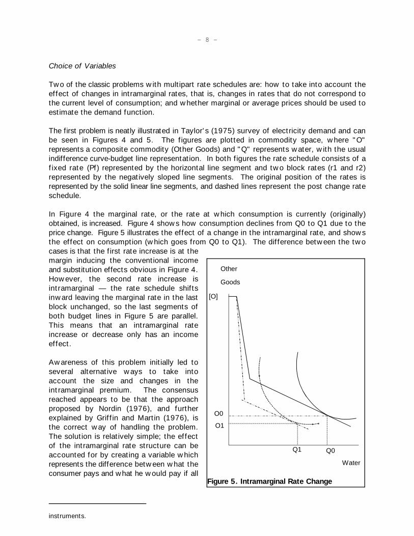
Figure 5. Intramarginal Rate Change

Choice of Variables

Two of the classic problems with multipart rate schedules are: how to take into account theeffect of changes in intramarginal rates, that is, changes in rates that do not correspond tothe current level of consumption; and whether marginal or average prices should be used toestimate the demand function.

The first problem is neatly illustrated in Taylor's (1975) survey of electricity demand and canbe seen in Figures 4 and 5. The figures are plotted in commodity space, where "O"represents a composite commodity (Other Goods) and "Q" represents water, with the usualindifference curve-budget line representation. In both figures the rate schedule consists of afixed rate (Pf) represented by the horizontal line segment and two block rates (r1 and r2)represented by the negatively sloped line segments. The original position of the rates isrepresented by the solid linear line segments, and dashed lines represent the post change rateschedule.

In Figure 4 the marginal rate, or the rate at which consumption is currently (originally)obtained, is increased. Figure 4 shows how consumption declines from Q0 to Q1 due to theprice change. Figure 5 illustrates the effect of a change in the intramarginal rate, and showsthe effect on consumption (which goes from Q0 to Q1). The difference between the twocases is that the first rate increase is at themargin inducing the conventional incomeand substitution effects obvious in Figure 4.However, the second rate increase isintramarginal — the rate schedule shiftsinward leaving the marginal rate in the lastblock unchanged, so the last segments ofboth budget lines in Figure 5 are parallel.This means that an intramarginal rateincrease or decrease only has an incomeeffect.

Awareness of this problem initially led toseveral alternative ways to take intoaccount the size and changes in theintramarginal premium. The consensusreached appears to be that the approachproposed by Nordin (1976), and furtherexplained by Griffin and Martin (1976), isthe correct way of handling the problem.The solution is relatively simple; the effectof the intramarginal rate structure can beaccounted for by creating a variable whichrepresents the difference between what theconsumer pays and what he would pay if all

- 9 -

For instance, Schefter and David (1985) argue that most studies use average consumption to13

calculate the intramarginal premium. This assumes that all consumers would be consuming at the blockcorresponding to the average consumption, which is unlikely to be the case. The correct variable is theaverage intramarginal premium rather than the intramarginal premium calculated at the average level ofconsumption.

water demanded was charged at the marginal rate.

Since the effect of changes in intramarginal rates is essentially an income effect, it followsthat the coefficients of income and the intramarginal premium should be roughly the same inabsolute value but with opposite sign. In empirical applications, however, few cases reportsimilar coefficients for income and the intramarginal premium. In fact, the overwhelmingmajority of reported results show coefficients that are significantly different.

This finding led to three types of reactions. Some have argued that water (or electricity) billsare so small relative to income that consumers will not look into the structure or changes inintramarginal rates. Consequently, consumers will not have a systematic response to changesin intramarginal rates. Others argue that in most studies the intramarginal effect is notestimated correctly, and this introduces a bias in the results. It is then concluded thatincorrect estimation explains why the theoretical prediction (equal coefficients) is notempirically verified. Another argument is that the intramarginal effect is so small that it is13

lost in the random influences that affect consumer behavior. Hence, it is not surprising to findthat the value of both coefficients differs (Westley 1981). Finally, other authors note thatmost demand estimates are based on aggregate data, so the prediction that the income andintramarginal premium effect will have the same size is no longer necessarily valid (e.g.Blattenberger 1977: 115-120).

Agnostic researchers who are skeptical about the premises of standard demand theory arguethat while a perfectly informed utility maximizing consumer should react to marginal, and notaverage price, few consumers may have a sufficiently detailed knowledge of the rate scheduleor care to acquire it because of information costs. They may exhibit behavior which is notin strict accordance with economic theory. Instead, consumers may use some average priceapproximation as a guiding rule of thumb for consumption decisions for what is, after all, agood that usually has a relatively small share in total family expenditure.

Demand estimation is a problem in applied economics, and theory can take us just so far. Forpractitioners, whether the consumer reacts to the size of (or changes in) the intramarginalpremium eventually becomes an empirical question. A refreshing aspect of some of the waterdemand literature is the notion that the potentially relevant variables for econometricestimation ought to include things the consumer can easily understand and decide on.Meaningful applied models have to sort out what is important from what is not. Waterconsumers may react to average prices, marginal prices, or even just their total monthly waterbill, and data can be used to help resolve the issue.

In this vein, Oppaluch (1984) developed a model (elaborated by Chicoine and Ramamurthy1986) that can be used to statistically test which price reaction alternative is supported bythe data. The starting point is a demand model like:

- 10 -

n-1 n-1 Q = " + $ P + $ P + $ {[E (P - P )Q ]/Q} + $ {Y - [E (P - P )Q ]} (12)1 x 2 n 3 i n i 4 i n i i=1 i=1

where:P = prices of other goodsxP = marginal price of water at block n, where consumption occurs nP = price of water at intramarginal block i<niQ = quantity of water at intramarginal block ii

The second term in (8) represents the marginal price of water, or the price of water at theblock where consumption occurs. The third term is the difference between average price andmarginal price and the last term is income minus the intramarginal premium. The averageprice for consumption up to block n is:

nP̄ = [E (P*Q )]/Q (13)i i i=1

Average price in Eq. (13) can also be expressed as:

n n-1[E P*Q ] + P (Q - E Q )i i n i i=1 i=1P̄ = ------------------------------------ (13.1)

Q

which can be transformed into an expression that includes a marginal price term and anaverage price term that is net of the marginal price:

n-1P̄ = P + [E (P - P )Q ]/Q (13.2)n i n i i=1

which are the second and third terms in Eq. (12). Restricted and unrestricted estimation ofEq. (12) allows the following statistical tests to be made (Chicoine and Ramamurthy 1986):

Test 1 Test 2

Null Hypothesis H0: $ = 0 $ = $3 2 3Alternative Hypothesis H1: $ Ö 0 $ Ö $3 2 3

Tests on Eq. (12) can yield the five different outcomes summarized in Table 1.

Other

Goods

Water

Q0Q1

O0

O1

[O]

O2

Q2

O2, Q2 and O1, Q1 = Multiple EquilibriaAfter Relative Price Change

- 11 -

Figure 6. Multiple Equilibria.

Table 1Possible Test Results

Test Results Conclusion

1. $ = 0 and $ =\ $ ===> Marginal Price Model3 2 3

2. $ =\ 0 and $ = $ ===> Average Price Model3 2 3

3. $ = 0 and $ = $ = 0 ===> No Price Response Model3 2 3

4. $ = 0 and $ = $ ; $ =\ 0 ===> Indeterminate Model3 3 2 2

5. $ =\ 0 and $ =\ $ ===> General "Decomposed" Price Model.3 2 3

In other words, if the coefficient of $ is significantly different from zero (and presumably2negative) while $ is not significantly different than zero (i.e. test result 1) the marginal price3hypothesis cannot not be rejected. If both coefficients are insignificantly different from eachother (i.e test result 2), then the average price hypothesis cannot be rejected.

Properties of the Demand Function

One of the most troublesome aspects ofdemand estimation when prices are set inmultipart block rates is that individualdemand functions may be discontinuous.This problem was first highlighted by Taylor(1975), and can be easily understood withthe following example. In Figure 6 we havea tariff schedule with a fixed charge andtwo unit tariff blocks. Initially, anindifference curve corresponding to a singlehousehold has tangency point at Q0. If theprice of the second block increases theconsumer would be indifferent between Q1and Q2, which means that the solution tothis problem is indeterminate. If we assumethat the choice is Q1, the demand curvewould have a "hole" corresponding to thepoints between Q1 and Q2. If this is thecase, it is not clear what sort of demandcurve can be estimated, or morefundamentally, which (if any) meaningfulproperties of demand systems would bevalid.

D1D2

D3

Price

Q 2 = Q fQ1 Q3

<----------------------------------------->Fixed Charge Block; Pmarg = 0

Water Consumed

Pmarg

------------------>Unit Price Block

Not Observed Observed

- 12 -

See Bohi (1981: 10-12 and 149-151) for an interpretation of elasticities estimated from aggregate14

data and bias in coefficients.

Figure 7. Sample Selection Bias.

In the applied literature, two explicit approaches have been proposed to circumvent thisproblem. The first one argues that aggregate demand functions are not discontinuous to theextent that different individuals have different tastes. By taking an average of a sufficientlylarge number of individuals, indifference curves can be presumed to be located along the rateschedules.

The main problem of this approach is that the aggregate demand curves estimated on thebasis of averages for groups of individuals no longer have the standard properties of individualdemand functions derived from consistent utility functions. The only properties that remainafter aggregation are homogeneity and budget exhaustion (Sonnenschein 1973).Interpretation of results in terms of elasticities is therefore unclear. In addition, it is frequentlyfound that estimates based on averages tend to overstate demand price elasticities.14

The second solution to the problem of discontinuity is somewhat roundabout, and has beenproposed by Wade (1980). This approach consists of estimating demand indirectly throughestimation of the parameters of a Stone-Geary utility function. Once the parameters of theutility function are identified, demand can be calculated using any appropriate optimizationalgorithm. In this approach the existence of "holes" is still possible, although the quantitiesof water demanded can always be estimated in a manner consistent with utility theory. Inthis approach, the concept of price elasticityis transformed into a weighted average ofelasticities on different blocks.

In our Argentina application the data arefrom a cross-section of communities, mostof which have increasing block rateschedules. Therefore the kinked demandproblem is not serious, and does not affectthe estimation techniques for thisapplication, or the interpretation of results.We therefore do not dwell on the issuefurther.

Sample Selection Bias

Sample selection bias may be importantwhen some sampled consumers are not inthe block rate schedule, but instead only paya fixed charge for quantities of water belowsome statutory minimum that triggers blockrate pricing on a per unit consumed basis(Wade 1980). (Chicoine and Ramamurthy(1986) note the possibility of sample

- 13 -

selection bias, but do not correct for it.) In this case it appears on the surface that marginalprice can be set to zero and the fixed charge customers included in the estimation sample.However, more properly, marginal price is not necessarily zero — indeed it is not observed atall for a potentially large number of fixed charge customers with demands characterized byschedule D2 in Figure 7. Their observed behavior contains no useful information on therelationship between marginal willingness to pay (equals marginal price) for alternativequantities of water below the trigger quantity in equilibrium. Figure 7 shows threerepresentative consumers who differ by level of income. Consumers with demand curves D1and D2 are not in the rate schedule and do not pay an observed marginal price, while theconsumer with demand curve D3 can equate marginal willingness to pay with the unit priceby consuming at Q3.

If the fixed charge customers who are not in the block rate schedule are deleted from theestimation sample and the demand relation is estimated using only the observations fallingwithin the block rate schedule where unit prices and their corresponding quantities areobserved, OLS or IV estimators may produce biased and inconsistent parameter estimates.The simple reason is that the expected value of the error term in the demand equation forobserved consumers falling in the block rate schedule is likely to be non-zero, violating theusual assumption.

Because sample selection bias is the most difficult issue to understand and deal witheconometrically, its origins and the methods that can be used to handle it are explained insome detail. Only then is the additional complication of simultaneous equations in a sampleselection framework introduced, and a consistent technique for estimation of the parametersof the structural water demand relation proposed.

Problems with Ordinary Least Squares, even in the Absence of Simultaneity

For simplicity, suppose we set aside the issue of simultaneity by assuming that rate schedulesoffer water at a constant per-unit price (Pmarg) once some consumption threshold (Qf) hasbeen crossed, instead of being step functions beyond the threshold. Also assume two typesof consumers — households with a strong demand for water whose demand schedule is, forreasons of income, wealth, or taste, located above (to the northeast of) the demand scheduleof a second category of users with a weaker demand for water. In this example, the highincome households pay the lump sum customer charge and a marginal rate as well becausetheir demand schedule pulls them into the region of the rate schedule. But low incomehouseholds pay only the lump sum charge and consume whatever the household requiresbelow the Qf threshold based on the role of exogenous socioeconomic variables other thanprice, Pmarg.

The analyst only observes the price-quantity relationship for the first, wealthier class ofconsumer falling in the block rate schedule. The less well-off customers array themselvesalong the Pmarg = 0 axis below the Qf threshold. While their willingness to pay for thequantities they are known to consume cannot be observed, there is a hypothetical marginalprice that would validate or call forth these quantities. Some of the families below Qf will usewater until its marginal value is truly zero, where their demand schedule cuts the horizontalaxis (D1 in the Figure). But other families may have demand schedules that are everywherebelow the prevailing rate schedule, and will consequently be clustered around the threshold

- 14 -

See Wade 1980 for a numerical example and an attempt to correct the problem using the Tobit15

estimator.

For an innovative approach that can be used to augment the sample of public water utility customers16

in the rate schedule with additional information on unconnected customers paying high prices to privatesuppliers (tank trucks) and consuming low quantities relative to public utility customers, see Gómez(1987). In essence, Gómez's method provides information on legitimate price/quantity pairs for familieslike those in the public utility's fixed charge part of the schedule (e.g. segments of D1 and D2 in Fig. 7above Pmarg=0) where such information is not observed. However, this method does not solve thesimultaneity bias or sample selection problems.

Qf (shown as D2 in the Figure). With random error in the data, there is no way to easilydistinguish between these two cases. The true demand schedule for these poorer families15

is unobserved because of the artifact of the two-part (lump sum cum unit rate) tariffschedule.16

While the analyst would like to have price observations for the consumer group in the fixedcharge category below Qf, these are not observed. Pmarg could be coded as equal to zerofor each and every consumer in that category, but unfortunately zero has no economiccontent or meaning for a subset of the observations below Qf. It is merely a convention thatindicates a missing value for Pmarg.

Of course, in estimation one could proceed following the above convention, replace theunobserved prices with zero, and estimate the demand function over the full sample ofcustomers in both classes as if an unavailable marginal willingness to pay value was a truezero. The consequence of so doing, given any set of exogenous variables, would be to pullthe estimated price intercept down from the true intercept and to decrease the estimated priceslope relative to the true slope. The result would be a false hybrid demand function.

Another approximation would be to construct a marginal price proxy for observations belowQf by dividing the fixed charge paid by the quantity actually consumed. Again, just likesetting Pmarg to zero, there is no guarantee that this average price proxy will correspondclosely with the true marginal willingness to pay measure for price.

A final, and more reasonable approach would be to estimate the demand relation only fromobservations falling in the rate schedule (i.e. Q > Qf) discarding all fixed-charge-onlyobservations where marginal price is not a decision variable and is not observed.Unfortunately, the parameters estimated from this censored sample by OLS may beinconsistent. This arises because the expected value of the error in such an OLS regressionis non-zero, violating full ideal conditions of the classical normal linear regression model (seeGreene 1990). As discussed next, a correction technique exists to produce consistentdemand function parameter estimates.

The Heckman Approach: Sample Selection Bias Correction with no Simultaneous Equations

For the moment treating marginal price as exogenous, the full sample of water consumers canbe separated into those not in the rate schedule for whom marginal price is not observed andthose in the rate schedule paying an observed marginal price. Consider the following tworegime three-equations model (Heckman, 1979, Lee and Trost 1980, Mullahy 1986):

- 15 -

Regime 1. Rate Schedule Demand. Q $ Qfi

Q = X '$ + Pmarg $ + u iff Z( $ u (14)1i 1i 1 2 1i i i

Regime 2: Fixed Charge Demand. Q < Qfi

Q = X $ + u iff Z( < u (15)2i 2i 3 2i i i

Regime 3: Selection/Latent Demand

Q = Z( + u ; u = N(0, 1) (16)*3i i 3i i

where Q is the amount of water consumed, X , X , and Z are row vectors of exogenous.i 1 2 iexplanatory variables, and Q represents the difference between the unobserved quantity of*

3iwater desired and the minimum threshold Qf. If this difference is positive, the consumercrosses the threshold into the rate schedule; if it is negative the consumer pays only a fixedcharge to consume an amount below Qf.

Here the quantity of water demanded if a user is in the rate schedule, Q , is greater than the1iquantity demanded if the user pays no marginal price, Q , and belongs to the fixed charge2iregime. Given the exogenous variables X , X , Z (and for now Pmarg ) the sample of rate1i 2i i ischedule customers is observed only if Q is positive; that is if the unobserved intensity of*

3idesire to consume water passes beyond the Qf threshold defining the point of entry into theirate schedule. Otherwise, the unobserved intensity of desire measure falls below Qf and aimarginal price/quantity consumed equilibrium pair are not observed. Instead in the secondregime only fixed charge demand Q is observed.2i

In this model the latent measure Q is unobserved. But since the variables it relates to (the*3i

Zs) are, a discrete indicator can be constructed from the data by observing which regime eachobservation belongs to:

I = 1 for Q > 0 (Regime 1) (17)i 3i*

I = 0 otherwise (Regime 2)i

In other words, usable price-quantity pairs are available to the analyst only when I = 1because latent indicator exceeds the Qf defining the threshold of entry into the rate schedule.

If the error terms in the demand equation and the intensity equation are correlated with zeromeans and covariance F Heckman considers the expectation E (Q * I = 1) which can be13 1i iwritten:

E (Q * I = 1) = X $ + Pmarg $ + E (u * I = 1) (18)1i i 1i i 2 1i i

where the notation (* I = 1) refers to the sample selection rule, "conditional on being in theirate schedule."

Consider least squares estimation using only those observations which qualify given the rulein Eq. (16). If OLS is performed on (14), will consistent parameter estimates result? Theanswer from the sample selection literature is in general, no, unless u is independent of u1i 3i

- 16 -

Note that the standard deviation F cannot be estimated, so it is conventionally set to one. Therefore1733

the covariance term F between F and F is conventionally expressed as DF F where D=corr[u ,u ].13 33 11 33 11 1 3

Therefore, F =DF . 13 11

so the conditional expectation of u is zero and F equals zero. This is true because it can1i 13be shown (Heckman 1979, Lee and Trost 1980, Olsen 1980, Mullahy 1986) that theexpected value of the error in the rate schedule demand equation is not zero:

E(u * I = 1) = F 8 (19)1i i 13 i

Here, F is the covariance between the error terms in the rate schedule demand function13(Regime 1) and the selection decision (Regime 3). The term 8 is the ratio of the standard17

inormal probability density (N) evaluated at Z to the standard normal distribution function (M,ior the probability that observation i belongs in Regime 1) evaluated at the same point (8 isicalled the Inverse Mills Ratio). If an observation has a high probability of containing usefuldata for Regime 1, its value for 8 will be small and positive. Therefore, selectivity bias wouldbe unimportant if all the 8 were negligibly small and positive because the probability of sampleiinclusion is high for all observations. Also, unless the covariance between the Regime 1demand equation and the latent indicator equation is zero (i.e. F =0), OLS on Eq. (18) will13yield inconsistent parameter estimates because E(u * I = 1) includes the disturbance but OLS1i iignores it under the false assumption that E(u )=0.1i

Heckman's suggested procedure to estimate Eq. (18) consistently proceeds in two steps. Inthe first step a Probit model is estimated on the binary indicator I defined by Eqs.(16) andi(17), producing consistent estimates of the ( parameter vector. Then for each observationan estimate of lambda, 8, can be constructed and employed as a regressor in Eq. (18) aboveiusing the data from the subsample in Regime 1. The second stage regression is:

Q = X $ + Pmarg $ + 8 $ + V (20)1i 1i 1 i 2 i 3 i^

where V is an error term with mean zero and $ is an estimate of F = DF . Note that OLSi 3 13 11estimates on the Regime 1 sample which ignore sample selection would not include 8̂ as airegressor.

Extension of the Sample Selection Model to the Simultaneous Equations Situation

Relaxing the assumption that the rate schedules (in a cross sectional sample of consumers indifferent localities) are characterized by constant prices per unit of consumption introducesthe complication of block rate pricing. As explained earlier, this raises the distinct possibilityof simultaneous equations bias because marginal price (when it can be observed) is no longerexogenous, but is chosen by each consumer simultaneously with consumption quantity (whenit can be observed). The solution to this additional complication is the extension ofinstrumental variable methods to the sample-separation case generally characterized by twosimultaneous equations systems corresponding to the two different regimes and a selectivitycriterion determining the regime to which the observations belong (Lee, Maddala and Trost1980).

- 17 -

There are j dummy variables, equal to the number of communities in the sample minus one if an18

intercept is in the supply equation. Obviously if the sample included only one community and one timeperiod, the demand function could not be identified.

Under these circumstances, and ignoring the fixed rate regime (because the endogenous priceand quantity variables corresponding to the demand function are only observed when I = 1),ithe simultaneity appears only in Regime 1. With simultaneity, and a cross-sectional sample,Regime 1 is now expanded by adding a multi-location block rate supply-side equation to thesystem along with the demand equation and the probit selection criterion function.

I. Regime 1

Demand

Q = X $ + Pmarg $ + u (21)1i 1i 1 2 1i

Supply

Pmarg = L [P][B] + u (22)i 2i

II. Probit selection criterion

PROB (I = 1) = 1 - F(-Z() = 1 - M(-Z() = M(Z() (23)i i i i

Here for any individual, i, X is a 1 x k row vector of exogenous explanatory variables as1ibefore; $ , is a k x 1 column vector of demand parameters; $ is the parameter on price; L is1 2a 1 x j column vector of j localities; P is a j x m matrix which represents the price per cubicmeter of water paid in each location at m different consumption intervals; B is an m x 1column vector which identifies the block chosen by the consumer; and Z is a 1 x j row vectoriof explanatory variables determining whether an observation belongs in Regime 1 (price andquantity pairs observed) or not; and F ( ) is the cumulative normal distribution function.

evaluated at Z( for the Probit, PROB indicating probability.i

On the supply side, the entire across-community block rate structure can be written exactlyby the analyst with prior knowledge from the rate schedule step functions reporting B and P.Nevertheless, the analyst does not know a-priori with any certainty which of the P rates willbe chosen by any individual, so the B variable is endogenous in this model — e.g. any B mustmfall somewhere in one of the blocks defined by B. So the exogenous variable on the supplyside is the location dummy variable represented by L.18

To estimate the structural parameters $ , $ of the demand relation in this model the1 2instrumental variable approach outlined in Lee, Maddala, and Trost can be used. It is directlyanalogous to two stage least squares with the addition of an estimate of the Mills Ratio 8i(constructed from the Probit equation) as an extra instrument.

The estimation steps are (Lee, Maddala, and Trost 1980):

- 18 -

1) Estimate the Probit criterion equation and construct an estimate of the Inverse MillsRatio 8 for each individual known to be in the rate schedule.i

2) Estimate a reduced form equation for marginal price, Pmarg, using all exogenousexplanatory variables in the Regime 1 system (X , L) as instruments along with the 81i ifrom step 1.

3) Predict the instrument for marginal price using the equation estimated in step 2.

4) Estimate the demand equation on the Regime 1 sample using the exogenousexplanatory variables X , the constructed instrument for Pmarg from Step 3, and the1iconstructed Inverse Mills Ratio 8 from Step 1. The former accounts for theiendogeneity of price and the latter for sample selection bias, just as before.

Model Specification and Data

Supply Variables

The first step in estimating water demand functions for Argentina was to find or createexogenous variables that could represent supply schedules and circumvent simultaneity. Forthis purpose we considered variables that could be used to estimate marginal prices andsubsequently use the prediction to estimate demand. Initially the following candidates wereconsidered:

a. Average Marginal Price: represented by the slope of a linear approximation to the totalrevenue schedule of each locality, as proposed by TBR.

b. Marginal Rate Schedule (P): represented by the rate charged per cubic meter of waterin 16 consumption block intervals common to all localities, as proposed by Westley(1984).

c. Locality Schedule (L): represented by dummy variables identifying each locality.

d. Block Schedule (B): represented by dummy variables identifying the block in whicheach household is consuming in the respective rate schedule.

Examples of the last three types of variables are shown in the following tables. Table 2shows hypothetical rate schedules for three localities, that is, the cost per cubic meter ofwater at different consumption intervals. Using the information from the top part of Table 2,rate schedules (P) can be calculated as shown in the lower part. Note that in this hypotheticalexample each rate schedule is defined by four variables, each one corresponding to aconsumption interval. In the sample rural localities in Argentina there were sixteen commonintervals with at least one different marginal price each (sixteen rate schedule variables). Twoof them had to be discarded because they turned out to be linear combinations of other rateschedules, so the final number of variables representing the rate schedule was fourteen.

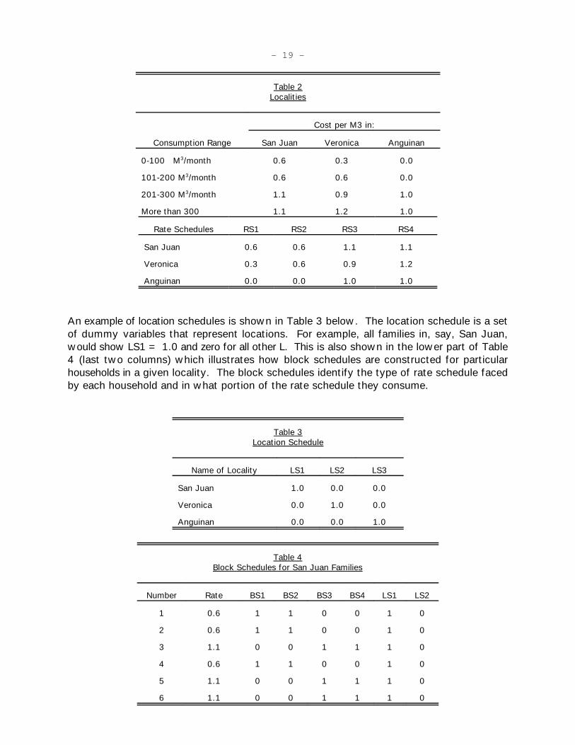
- 19 -

Table 2Localities

Cost per M3 in:

Consumption Range San Juan Veronica Anguinan

0-100 M /month 0.6 0.3 0.03

101-200 M /month 0.6 0.6 0.03

201-300 M /month 1.1 0.9 1.03

More than 300 1.1 1.2 1.0

Rate Schedules RS1 RS2 RS3 RS4

San Juan 0.6 0.6 1.1 1.1

Veronica 0.3 0.6 0.9 1.2

Anguinan 0.0 0.0 1.0 1.0

An example of location schedules is shown in Table 3 below. The location schedule is a setof dummy variables that represent locations. For example, all families in, say, San Juan,would show LS1 = 1.0 and zero for all other L. This is also shown in the lower part of Table4 (last two columns) which illustrates how block schedules are constructed for particularhouseholds in a given locality. The block schedules identify the type of rate schedule facedby each household and in what portion of the rate schedule they consume.

Table 3Location Schedule

Name of Locality LS1 LS2 LS3

San Juan 1.0 0.0 0.0

Veronica 0.0 1.0 0.0

Anguinan 0.0 0.0 1.0

Table 4Block Schedules for San Juan Families

Number Rate BS1 BS2 BS3 BS4 LS1 LS2

1 0.6 1 1 0 0 1 0

2 0.6 1 1 0 0 1 0

3 1.1 0 0 1 1 1 0

4 0.6 1 1 0 0 1 0

5 1.1 0 0 1 1 1 0

6 1.1 0 0 1 1 1 0

- 20 -

For example, the family identified as number 1 consumes in a block that ranges from 0 to 200m /month. In this block the price is $0.60 cents per m and the family is located in locality3 3

number 1. In contrast, family 3, which lives in the same location, is consuming at a blockranging between 201 and more than 300 m /month at a price of $1.1 per m .3 3

Of these four variables, Westley's Marginal Rate Schedule (P) and the Location Schedule (L)were by far the best predictors for marginal price. All subsequent tests and IV regressions useone or another of these two variables as alternative instruments.

Demand Variables

Apart from the usual variables that appear in any demand function (price and income), datafrom the OEO survey contained information for several other indicators that could potentiallyexplain water consumption. These variables ranged from family attributes (number ofhousehold members, number of adults, number of children, etc.), family assets (ownershipof land, house, radio, television, etc.), type of sewerage facilities, sources and uses of water,water supply reliability, household water storage facilities, etc.

After carefully reviewing the information, some variables (and some individual surveys) werediscarded. With the reduced data set we tested the influence of different combinations ofvariables. Some of the attributes turned out to be highly collinear (e.g. assets and income);and many of the system attributes (e.g. sources and uses of water, type of sewerage system)were too uniform across the sample to be of any value in terms of additional information.These features of the sample reduced the number of usable variables to:

a. Marginal Price;b. Intramarginal Premium;c. Income;d. Number of adults in the household (Adults);e. Electricity Bill as a wealth proxy (Electricity);f. Number of water faucets inside the house (Faucets); and g. Average number of interruptions in service per month (Outages).

Water Demand Equation Specification

The specifications tested combine three types of variables: marginal price, intramarginalpremium and income, and other variables (number of adults, electricity bill, number of waterfaucets, etc., as listed above).

The marginal price is in all cases the per unit cost of water at the level where the householdis consuming. If the household is consuming at the minimum, fixed charge level, the marginalprice is set to zero.

The intramarginal premium is generally defined in the literature as the difference betweenwhat the consumer actually pays and what would have to be paid if all units consumed were

- 21 -

charged at the marginal rate. In our application the premium was calculated in two ways: asa lump-sum transfer, or as the difference between average and marginal prices.

In the first case the premium is a subtraction (or addition) to income. The theoreticalexpectation is that the coefficients from this type of premium and household income will bethe same but with opposite sign. In this formulation, the lump-sum also includes the fixedwater charge since this cost is a deduction from income related to the act of consumingwater, but divorced from the decision of how much to consume at the margin. In someapplications, the intramarginal premium is directly deducted from income, which means thatthe equality of coefficients for both variables is implicitly assumed.

The general model can therefore be estimated in two variants, with and without the constrainton the equality of the coefficients of the intramarginal premium and income. That is:

Model I. Unconstrained, Marginal Price, Inequality of Income and Premium Effect

Q = " + $ *Pmarg + $ *(Premium+Fixed Charge) + $ *Y + $*[Other]1 2 3 i

Model II. Constrained Income Effect Version of I.

Q = " + $ *Pmarg + $ *(Y-Premium-Fixed Charge) + $*[Other]1 2 i

A second formulation of the intramarginal premium, tailored to the Oppaluch test, is definedon a per unit of water basis. In this case consistency with the derivation of the modelspecification requires that we subtract from income all payments related to waterconsumption (including the fixed charge). Thus the specification would be:

Model III. Oppaluch's Marginal and Average Price Model.

Q = " + $ *Pmarg + $ *Pr + $ *(Y-Premium) + $*[Other]1 2 3 i

where Pr = Average Price - Marginal Price.

Each specification was estimated with two different samples: the full sample of 685 families,and the subset sample of 279 families consuming above the minimum, fixed charge level.Estimated demand functions for both samples using OLS and 2SLS are reported below for allfive model specifications.

The purpose of using different samples was to compare the effects of (erroneously) includingfamilies consuming at the minimum level without correcting for the lack of an appropriatemarginal price measure. Although the marginal price for these families is set to zero, theirconsumption level does not provide information on their price/quantity demanded choice(unless the marginal utility of consuming water for public system customers at the observedlevel is zero, or if the sample of public utility customers is augmented with privately suppliedlow income customers following Gómez 1987). The relative size of the bias introduced byusing data from households in the fixed charge block is not known a-priori, so it is interesting

- 22 -

Our sample only includes public utility customers, so the implications of Gómez's sample19

augmentation approach could not be empirically explored.

Other functional forms were explored, but our conclusions about simultaneity and sample selection20

bias remained robust across functional specification.

The only exception for signs is with Outages in the 2SLS results.21

to compare the results between both samples. Estimation using a smaller sample of19

consumers in the unit price part of the rate schedule beyond the fixed charge block is a wayof correcting this problem. In contrast, the comparison between OLS and 2SLS resultsillustrates the effects of simultaneous equations bias and sample selection bias.

Estimation Results

The following tables present the estimation results, which all maintain the hypothesis of alinear demand function. We start with a comparison of OLS models using the full sample20

of 685 observations, shown in Table 5. These OLS results are generally very poor. The signsof the price and income coefficients are in most cases wrong or insignificantly different fromzero, which is evidence of the twin effects of simultaneous equation bias and the impropercoding of marginal prices in the fixed charge block as zero. In contrast, the signs of othervariables are always correct, often significant and do not change much compared to the onesestimated using 2SLS.21

- 23 -

Table 5OLS Full Sample Results

(Absolute Value of "t" Statistic in Parentheses)

Model I II III

Constant 12,588.8 9,441.0 9,388.4(13.5) (11.4) (11.4)

Marginal Price -590.3 4,370.0 6,179.7(0.5) (5.9) (4.5)

Premium -498.9 - 20,093.6(6.5) (1.5)

Income -0.1 -.4 -0.4(0.6) (1.6) (1.8)

Adults 257.6 387.0 379.5(1.5) (2.2) (2.1)

Faucets 306.2 352.0 357.0(2.6) (2.9) (2.9)

Outages -729.0 -165.0 -92.9(1.2) (0.3) (0.1)

Electricity 68.9 61.3 60.5(5.8) (1.6) (4.9)

R 0.18 0.12 0.122

F 21.5 16.9 14.9

Note: Marginal price in fixed charge block coded as zero.

Results using 2SLS on the Full Sample with two different instruments (P or L) for the rateschedule are shown in Tables 6 and 7.

Marginal prices show correct coefficients (except in Model III with the P instrument) and aregenerally significantly different from zero. The elasticity values for prices, premium andincome are low, which is a result consistent with the bias introduced by including families inthe minimum consumption category. For example, the highest price elasticity value is only-0.12, the highest elasticity of the intramarginal premium is -0.08 (Table 7, Model I) andincome coefficients have correct results only in one case (Model I).

As mentioned above, the values of the coefficients for all other variables (with the exceptionof service interruptions, Outages) are not significantly affected when estimated with 2SLS.The constant term in both cases roughly corresponds to a consumption level of about 330liters per connection per day. This is reasonable since the average household size is between3 and 4 people and the average per capita consumption level in the sample is close to 100liters per persons per day. For the same reason, the coefficient on the number of adults in thehousehold (Adults) is also rather low, because it implies that adding or taking away one adultfrom the household will change daily consumption by about 10 to 20 liters per day.

- 24 -

Table 62SLS Full Sample Results With Location Dummy Variable Instrument

(Absolute Value of "t" Statistic in Parentheses)

Model I II III

Constant 11,720.0 9,833.7 10,013.5(11.1) (11.4) (11.0)

Marginal Price -4,690.0 -1,977.0 -8,115.0(3.2) (1.7) (1.5)

Premium -302.0 - -6,789.0(3.0) - (1.2)

Income .0 -0.05 -0.05(0.0) (0.2) (0.02

Adults 303.0 381.1 405.9(1.7) (2.1) (2.1)

Faucets 383.0 414.3 404.7(3.1) (3.3) (3.1)

Outages -225.3 129.0 -99.7(0.0) (0.2) (0.1)

Electricity 86.4 82.8 86.5(6.7) (6.3) (6.2)

Elasticities:Ep -0.08 -0.03 -0.13Epr -0.07 - -0.08Ey n.s. n.s. n.s.

n.s.= Result is not significant.Note: Marginal price in fixed charge block coded as zero.

It is difficult to judge the reasonableness of the size of other coefficients. The coefficient onFaucets indicates a relationship between the number of inside faucets and water consumptionsimilar to the effect of the number of adults on monthly water consumption. Frequency ofservice interruptions (Outages) in most cases has the anticipated negative sign in OLS and thewrong sign in 2SLS, but is generally insignificant using either estimator. Finally, the value ofthe electricity bill (as a proxy for wealth) indicates a positive relationship between wealth andwater consumption, with an average elasticity of about 0.15. In terms of price and incomecoefficients the main change from OLS to 2SLS is that the price, premium and incomecoefficients take on the theoretically expected signs, even though the elasticities are low.

Oppaluch's test (Model V) is inconclusive. In OLS the price and premium coefficients are bothsignificant, and significantly different from each other, but have the wrong sign. In 2SLS bothparameter estimates are insignificantly different from zero at the 95% level, implying no priceresponse. An important implication of these results is that if we estimate with the full sampleof observations, OLS will not yield correct results, while 2SLS yields low but theoreticallyconsistent elasticities for the models maintaining a marginal price hypothesis.

- 25 -

Table 72SLS on Full Sample With Rate Block Dummy Variable Instrument

(Absolute Value of "t" Statistic in Parentheses)

Model I II III

Constant 12,164.0 9,940.0 9,817.1(10.5) (11.1) (10.8)

Marginal Price -7,146.0 -3,697.0 348.8(4.0) (2.7) (0.05

Premium -353.0 - 4,363.8(2.9) - (0.7)

Income .09 -0.05 -0.16(0.4) (0.2) (0.6)

Adults 288.2 379.6 364.6(1.6) (2.0) (1.9)

Faucets 397.6 431.0 437.6(3.1) (3.3) (3.4)

Outages -192.7 209.0 348.0(0.3) (0.3) (0.5)

Electricity 93.8 88.6 86.1(6.9) (6.5) (6.1)

Elasticities:Ep -0.12 -0.06 n.s.Epr -0.08 - n.s.Ey n.s. n.s. n.s.

n.s.= Result is not significant.Note: Marginal price in fixed charge block coded as zero.

Table 8 presents the results of applying OLS and 2SLS to the subsample of 279 familiesconsuming above the minimum, fixed charge consumption level instead of the entire sampleof 685 households. The results are interesting. First, in contrast to the results using the fullsample, the price coefficients (and corresponding elasticities) estimated with OLS using therestricted sample are not too different from the ones calculated using 2SLS. Second,elasticities and price coefficients are much higher in this sample. The price elasticity rangesbetween -0.2 and -0.4 (compared to -0.04 to -0.12 with the full sample). Third, the size andsignificance of the premium coefficients is erratic. The results of the Oppaluch test (modelIII) are particularly inconclusive since the price and premium parameters are significant in OLS(price with the wrong sign) and insignificant in 2SLS. Fourth, income coefficients aresignificant and have the correct sign in model I, although the elasticity value (0.02) stillappears to be low.

The most important general result of this group of regressions is that the effects of sampleselection bias have a greater impact than the simultaneity problems in this particular case.In other words, within the subsample of consumers that are above the minimum level, theeffects of simultaneity are very small. This is most likely because the distribution around the

- 26 -

In Table 9, only the unconstrained models (I and II) using marginal price as the consumer's decision22

variable can rightly be tested since the introduction of incorrect parameter restrictions as maintainedhypotheses would distort the test.

different rate schedules is more concentrated in one or two blocks per community, such thatin several cases the supply schedule is almost perfectly elastic.

Table 8Small Sample Results

(Absolute Value of "t" Statistic in Parentheses)

Model I II III

OLS 2SLS** OLS 2SLS** OLS 2SLS*

Constant 24,508.0 23,927.0 19,830.0 20,104.6 19,495.9 20,087.1(21.8) (21.2) (15.8) (16.0) (17.5) (16.5)

Marginal price -14,262.0 -13,629.0 -8,077.0 -8,648.0 14,804.0 -5,459.0(12.7) (11.7) (6.9) (7.1) (5.2) (1.2)

Premium -942.4 -789.9 - - 25,641.5 3,646.8(11.0) (9.0) - - (8.6) (0.7)

Income .39 .33 -.03 -0.01 -0.63 -0.1(1.8) (1.5) (0.1) (0.0) (2.7) (0.4)

Adults 3.3 51.0 260.0 270.0 249.3 269.8(0.0) (0.2) (1.0) (1.1) (1.1) (1.1)

Faucets 92.4 126.0 301.0 300.5 225.1 290.3(0.7) (1.0) (2.0) (2.0) (1.7) (2.0)

Outages -1,514.9 -1,338.0 -550.0 -518.0 680.8 -340.6(2.0) (1.7) (0.6) (0.6) (0.8) (0.4)

Electricity 48.8 49.2 49.6 50.1 28.0 47.1(4.4) (4.4) (3.7) (3.8) (2.3) (3.5)

ElasticitiesEp -0.45 -0.43 -0.26 -0.27 0.47 -0.17Epr 0.04 0.03 - - -0.62 -0.09Ey 0.02 0.02 -0.0 -0.0 -0.03 n.s.

R2 0.44 0.20 0.2030.90 11.00 9.60

** Using the Location Schedule dummy variable as an instrument.

The presence of simultaneous relationships was also tested with the Reset and Hausmantests. The former is a general specification which may capture problems other thansimultaneity while the latter is specifically testing for simultaneity. The results in Table 9generally support the view that the presence of simultaneity cannot be rejected. Most of theReset tests indicate the presence of specification problems while all but two of the Hausmantests confirm that simultaneity cannot be rejected.22

- 27 -

Table 9Tests for the Presence of Simultaneity: Small Sample

I. Using the Location Dummy Variable Instrument

1. Without Sample Selection Correction (Without Lambda)

Model I Critical Value

Reset (2) 12.86 3.84

Reset (3) 11.85 3.00

Reset (4) 8.04 2.60

Hausman 34.57 15.50

2. With Sample Selection Correction (With Lambda)

Reset (2) 14.67 3.84

Reset (3) 12.02 3.00

Reset (4) 8.15 2.60

Hausman 33.93 15.50

II. Using the Rate Schedule Dummy Variable Instrument

1. Without Sample Selection Correction (Without Lambda)

Model I Critical Value

Reset (2) 12.86 3.84

Reset (3) 11.85 3.00

Reset (4) 8.04 2.60

Hausman 1.06 15.50

2. With Sample Selection Correction (With Lambda)

Reset (2) 14.63 3.84

Reset (3) 12.01 3.00

Reset (4) 8.15 2.60

Hausman 4.34 15.50

Note: Numbers in parenthesis after Reset indicate powersof predicted independent variable used in test.

The results of Lee, Maddala and Trost's adaptation of Heckman's estimation procedure to thesimultaneous equations case are presented in Table 10.

- 28 -

For brevity, the first stage Probit estimation results used to produce observation-specific values of the23

Mills Ratio are not presented. The independent variables included in the Probit step were locationdummies, the proportion of income allocated to the fixed water charge, the upper limit of the fixedcharge block (in m per month), the number of adults in the household, the average hours of system3

outage per month, and the monthly electricity bill, a proxy for wealth. Marginal prices were notsignificant, and were not included.

Table 10Simultaneity and Selectivity Correction: Small Sample withHeckman's Two-Step Estimation and Instrumental Variables

(Absolute Value of "t" Statistic in Parentheses)

Model I II III

Constant 24,038.0 19,970.0 19,442.7(18.6) (14.8) (14.9)

Marginal Price -13,611.0 -8,981.0 -6,586.0(11.0) (7.4) (1.4)

Premium 796.0 - 2,693.0(9.0) - (0.5)

Income 0.33 -.03 -0.10(1.5) (0.1) (0.5)

Adults 54.7 266.0 227.8(0.2) (1.0) (1.0)

Faucets 121.0 352.0 318.0(0.8) (2.4) (2.1)

Outages -133.9 -554.0 -426.1(1.6) (0.6) (0.5)

Electricity 48.6 55.9 52.2(4.0) (4.1) (3.7)

Lambda -194.0 1,500.0 1,431.1(1.3) (1.9) (1.7)

Elasticities:Ep -0.43 -.28 -0.10Epr +0.03 - n.s.Ey 0.02 n.s. n.s.

n.s.= Result is not significant.

The results in Table 10 are similar to the results obtained with 2SLS in the small sample.23

Price elasticities range from -0.10 to -0.43; premium elasticities range from -0.05 to 0.03; andincome elasticities range from -0.01 to 0.02. All three models estimated yield theoreticallyconsistent elasticities for price. However, Model I yields positive premium elasticities (whichis incorrect), while models II and III yield insignificant (and negative) income elasticities.

In sum, better results were obtained using the subsample of individuals above the minimumconsumption under both OLS and 2SLS. Instrumental variables estimation with a sampleselection correction on this truncated sample is preferable on a-priori grounds, but did not

- 29 -

This method is used in Gómez (1987).24

introduce startling changes in the parameter estimates. The advantage of ignoringsimultaneity and sample selection bias by OLS estimation on the truncated sample issimplicity. Its disadvantage is that these problems may be non-trivial in some applications.Also, in many rural areas a large percentage of the population is in the minimum consumptionlevel, and OLS (or 2SLS) estimation on the truncated sample discards information on them byonly using families above that level in estimation. The Lee, Maddala, and Trost estimationmethod makes better use of all the sample information.

Conclusions

The results of estimating water demand functions from a sample of households connected topublic water systems in rural communities in Argentina yield some useful answers to thequestions posed at the beginning of this paper.

Simultaneous Equation Bias Exists

It is clear, both from theory and our Hausman tests, that there is a simultaneous equation biaswhen using OLS in the face of block-varying tariff schedules. The impact of this bias isstronger when the entire sample spanning the fixed and unit price tariff blocks is used thanit is when estimating with the smaller sample that excludes observations in the fixed chargegroup. But even in the latter case simultaneous equation bias could not be rejected.Therefore, at a minimum, any estimation of water demand should explore an instrumentalvariables approach (e.g. 2SLS) to try to produce consistent estimates of the price coefficients.

Using OLS on a sample of observations from a single locality and time period that containsboth public utility customers and unconnected customers supplied through low volume, highercost alternatives remedies the problem of unobserved information about low incomecustomers in the fixed charge part of the utility's rate schedule. But, it does not solve the24

simultaneous equation bias problem. As long as we are confined to a single locality and timeperiod, the use of OLS potentially is as likely to identify a demand as a supply curve, or withluck, some hybrid mixture of both that has a negative price parameter.

Average Price May not be Relevant

With respect to the choice of average versus marginal prices, the results of the Oppaluchspecification are not decisive. But, the results in Tables 8 and 10 suggest that marginal, notaverage, price is the relevant variable, since marginal price is significant at the 90% levelusing the critical value for a one-tailed test that does not admit the possibility of a positivemarginal price response. The intramarginal premium is in most cases not significantly differentfrom zero. Thus, the average price hypothesis cannot be accepted with our data set.

- 30 -

The expected value of any individual's quantity demanded q , given the values of its row vector of25i

regressors x , and conditional on being in the rate schedule (where ß is a row vector of parameteriestimates on variables other than 8) is:

E[q |x , q $ 0] = x'ß + ß 8i i i i 8 i

Sample Selection Bias May Matter

Sample selection bias may be important, as suggested by the borderline statistical significanceof the parameter attached to the Inverse Mills Ratio (the Lambda parameter) in Models II andIII of Table 10. Again, however, the results are not clear-cut. Several observations are inorder here.

The price coefficients obtained using the Lee, Maddala and Trost estimation method reportedin Table 10 do not appear too dissimilar from those obtained using 2SLS in the small sample.Since the Inverse Mills Ratio was estimated independent of prices, the conditional pricederivative of consumption (i.e. the price derivative of those within the block rate schedule) isunaffected by its presence in the conditional demand function. But, the estimate of theexpected value of water consumed, conditional on being in the rate schedule, is a function ofthe Inverse Mills Ratio, which can be thought of as an adjustment to the intercept thatdepends on the household's characteristics. 25

Depending on the data, the sample selection adjustment could have an impact on thecalculation of benefits accruing from a supply price reduction across consumers, since theposition of the demand schedule is affected by the value of the Inverse Mills Ratio and theparameter estimate attached to it. In our rate schedule sub-sample, the average value of theInverse Mills Ratio is 0.5, so the adjustment adds up to about 0.5*1,500 = 750 cubic metersper month to the constant term in Model II. So corrected, these augmented intercepts areclose to the constant terms estimated from 2SLS on the small sample where marginal pricecan be observed. The hypothetical building of demand schedules for households not in therate schedule "as if" they faced marginal prices and no fixed charge could bring about a widerdisparity between the two approaches.

There are other reasons to prefer Lee, Maddala and Trost's instrumental variables version ofthe Heckman two-step procedure. It has the advantage of using the information moreeffectively than 2SLS on the small truncated sample. Finally, the parameter estimates of the2SLS estimator which ignores incidental truncation introduced by the fixed charge group (i.e.doing 2SLS on the unit block rate customers only) are, at least in theory, inconsistent.

What To Do?

In general, to identify the demand function, data on more than one locality in a single timeperiod or more than one time period at a single locality are needed. Individuals in the publicutility's fixed charge category should not be included in the estimation sample, since theirmarginal willingness to pay cannot be accurately observed, and is not necessarily zero.

- 31 -

Assume we discard all the information pertaining to the subsample of observations in the fixed charge26

regime (Regime 2) and retain only those in the rate regime (Regime 1), making the sample truncatedrather than censored. Also assume that the observed marginal price Pmarg is constant rather thandefined as an increasing or decreasing block rate, so simultaneity is not an issue. Suppose someregressors appear in the sample selection equation (Equation 16 above) but not in the demand equation(Equation 14). If these variables are included in the estimation of Equation 18 on the truncated sample,according to Greene 1983, consistent parameter estimates will be obtained for variables which belongonly in the demand equation and not in the selection equation. Variables shared by both equations willstill have inconsistent parameter estimates. If the demand equation and the selection equation do nothave any variables in common, inclusion of the variables from the selection equation in the demandequation estimation will produce consistent parameter estimates for the latter. This result from Greene(1983) is linked to Heckman's intuition (1976) that the effect of sample selection is that variables thatdo not belong in the regression appear to be statistically significant in equations fit on selected samples. It is of little help, because a-priori knowledge about which variables belong in each stage of the decisionprocess is usually not available.

For the estimation sample it makes sense to augment the truncated sample of public utilitycustomers in the unit price blocks of the rate schedule with information on unconnectedhouseholds using private (or self) supply sources. Preferably, their characteristics (particularlyincome, assets, and water consumption levels) should be similar to those of the families in thepublic utility's fixed charge category that have to be dropped from the demand estimationsample. In this way, legitimate high price/low quantity observations can be obtained. But,this group of unconnected customers is akin to a separate locality that, at least potentially,faces unit prices that depend on consumption quantity, so the potential for simultaneousequations bias in such an augmented sample combining connected block rate households andunconnected households still exists.

The likely severity of the simultaneity and sample selection problems can be assessed by aclose look at the data. For example, if a small proportion of the sample falls into the fixedcharge regime (or a fixed charge regime does not exist in the rate structures observed acrossspace or time) the sample selection correction may be unnecessary. If an overwhelmingmajority of the subsample in the rate schedule falls into the first unit price block, or the place(or time) varying schedules all have constant rates rather than block-declining or block-increasing rates, then for all practical purposes, simultaneity is a non-issue. If both of theseconditions are satisfied by the data, OLS may be acceptable.

If there is a fixed charge regime with constant unit pricing rather than block pricing,simultaneity is no problem, but sample selection bias might be. Estimation on the truncatedsample should attempt to account for it, either using Heckman's correction method, or anapproximation using an adjustment to OLS (e.g. see Greene 1983, Olsen 1980). 26

If there is no fixed charge regime, but the observations are arrayed across a wide range ofdifferent block-defined unit prices, an instrumental variables estimator like 2SLS would bepreferable. The need for it can be established via a Hausman test.

If it appears that simultaneity and sample selection both are present, at a minimum wesuggest that the analyst should disregard the fixed charge customers and use an instrumentalvariables estimator on the in-block household observations.

- 32 -

In sum, the characteristics of the particular case dictate the degree of econometricsophistication required for the estimation of plausible household water demand functions.Nevertheless, potential estimation problems should not be ignored altogether by theindiscriminate use of simple OLS when its assumptions do not apply.

References

Billings, Bruce E. and Donald E. Agthe. 1980. Price Elasticities for Water: A Case ofIncreasing Block Rates. Land Economics, Vol. 56, No.1.

Blattenberg, Gail R. 1977. Block Rate Pricing and the Residential Demand for Electricity. Phd.Dissertation. Ann Arbor, Michigan: University Microfilms International.

Bohi, Douglas R. 1981. Analyzing Demand Behavior, A Study of Energy Elasticities.Baltimore: The Johns Hopkins University Press, Resources for the Future.

Bohi, Douglas and Mary B. Zimmerman. 1984. An Update on Econometric Studies of EnergyDemand Behavior. Annual Reviews Energy 1984-9.

Charney, Alberta H. and Gary C. Woodard. 1984. A Test of Consumer Demand Response toWater Prices: Comment. Land Economics, Vol. 60, No. 4.

Chicoine, David L. and Ganapathi Ramamurthy. 1986. Evidence on the Specification of Pricein the Study of Domestic Water Demand. Land Economics, Vol 62, No. 1.

Dutta, M. 1975. Econometric Methods. Brighton, England: South-Western Publishing Co.

Foster, Henry S. and Bruce R. Beattie. 1979. Urban Residential Demand for Water in theUnited States. Land Economics, Vol. 55, No. 1.

Gómez, Christian. 1987. Experiences in Predicting Willingness to Pay for Water Projects inLatin America, Washington, D.C.: Inter-American Development Bank, Project AnalysisDepartment.

Greene, William H. 1983. Estimation of Limited Dependent Variable Models by Ordinary LeastSquares and the Method of Moments. Journal of Econometrics, Vol. 21, pp. 195-212.

. 1990. Econometric Analysis. New York: Macmillan.

Griffin, Adrian H. and William E. Martin. 1981. Price Elasticities for Water: A Case ofIncreasing Block Rates: Comment. Land Economics, Vol. 57, No.2.

Hanke, Steve H. 1978. A Method for Integrating Engineering and Economics Planning. Journalof the American Water Works Association. September, pp.487-91.

Hausman, J.A. 1978. Specification Tests in Econometrics. Econometrica, Vol. 46, No. 6, pp.1251-1270.

Heckman, James J. 1976. The Common Structure of Statistical Models of Truncation,Sample Selection and Limited Dependent Variables and a Simple Estimate for SuchModels. Annals of Economic and Social Measurement, Vol. 5, No. 4, pp. 475-492.

Heckman, James J. 1979. Sample Selection Bias as Specification Error. Journal of theEconometric Society, Vol. 47, No. 1, pp. 153-161.

- 34 -

Heckman, J. 1979. Sample Selection Bias as a Specification Error. Econometrica, Vol. 97,pp. 155-162.

Lee, Lung-Fei and Robert P. Trost. 1978. Estimation of Some Limited Dependent VariableModels with Application to Housing Demand. Journal of Econometrics, No. 8, pp.357-382.

, G. S. Maddala, and Robert P. Trost. 1980. Asymptotic Covariance Matrices ofTwo Stage Probit and Two Stage Tobit Models for Simultaneous Models withSelectivity. Econometrica, Vol. 48, pp. 491-504.

Lee, Terence R. 1969. Residential Water Demand and Economic Development. Toronto,Canada: University of Toronto Press.

Maddala, G.S. 1983. Limited - Dependent and Qualitative Variables in Econometrics,New York: Cambridge University Press.

Martin, William E., Helen M. Ingram, Nancy K. Laney, and Adrian H. Griffin. 1984. SavingWater in a Desert City. Baltimore: The Johns Hopkins University Press, Resources forthe Future.

Meroz, Avigdor. 1968. A Quantitative Analysis of Water Demand in Developing Countries.International Bank for Reconstruction and Development, Economics DepartmentWorking Paper No. 17.

Mullahy, John. 1987. "Economic Estimation of Microeconomic Recreation ParticipationModels" in Economic Perspectives. N.J. Rau, editor. London: University College, pp.91-149.

Nakamura, Alice and Masao Nakamura. 1981. On the Relationships Among SeveralSpecification Error Tests Presented by Durbin, Wu, and Hausman. Econometrica, Vol.49, No. 6., pp. 1583-1588.

Nieswiadomy, Michael L. and David J. Molina. 1991. A Note on Price Perception in WaterDemand Models. Land Economics, Vol. 67, No. 3.

Nording, John. 1976. A Proposed Modification of Taylor's Demand Analysis: Comment. The

Bell Journal of Economics, 7.

Olsen, Randall J. 1980. Approximating a Truncated Normal Regression with the Method ofMoments. Econometrica. Vol. 48, No. 5. July.

Oppaluch, James J. 1981. Block Pricing and Consumer Behavior. University of Rhode Island,Department of Resource Economics Staff Paper # 81-20.

Oppaluch, James J. 1984. A Test of Consumer Demand Response to Water Prices:Reply. Land Economics, Vol 60, No. 4.

- 35 -

Powers, Terry A. and Carlos A. Valencia. 1980. SIMOP Urban Water Model. Washington,D.C.: Inter-American Development Bank, Papers on Project Analysis No. 5.

Sonnenschein, H. 1973. Do Walras' Identity and Continuity Characterize the Class ofCommunity Excess Demand Functions? Journal of Economic Theory, 6.

Schefter, J.E. and E. L. David. Estimating Residential Water Demand under Multi Part TariffsUsing Aggregate Data. Land Economics, Vol 61, No. 3.

Taylor, Lester D. 1975. The Demand for Electricity: A Survey. The Bell Journal ofEconomics. 6, No. 1 (Spring).

, G. R. Blattenberger, and R. G. Rennhack. 1981. The Demand for Energy in theUnited States. Report to the Electric Power Research Institute RP 1098. Lexington,Massachusetts: Data Resources Inc.

. 1982. "Some Problems and Issues in Building Econometric Models of EnergyDemand", in Perspectives of Resource Policy Modeling: Energy and Minerals. RaphaelAmit and Mordecai Avriel, editors. Cambridge Mass.: Harper, Row, and Ballinger.

Vaughan Jones C., John J. Boland, James E. Crews, Frederick C. DeKay, and JohnR. Morris. 1984. Municipal Water Demand, Statistical and Management Issues.Boulder: Westview Press.

Wade, Steven Howard. 1980. The Implications of Decreasing Block Pricing for IndividualDemand Functions: An Empirical Approach. Ph.D. Dissertation, University of Arizona.

Westley, Glenn. 1981. "The Residential and Commercial Demand for Electricity in Paraguay",Papers on Project Analysis No. 19, IDB, Washington D.C.

Westley, Glenn. 1984. "The Residential and Commercial Demand for Electricity in CostaRica", Papers on Project Analysis No.24. Washington D.C.: Inter-AmericanDevelopment Bank.

Williams, Martin. 1985. Estimating Urban Residential Demand for Water under AlternativePrice Measures. Journal of Urban Economics, 18.

and Byung Suh. 1986. The Demand for Urban Water by Customer Class. Applied Economics, 18.