Quantifying Coefficient of Thermal Expansion Values of Typical Hydraulic Cement Concrete Paving Mixtures

Final Report Submitted to

The Michigan Department of Transportation

Construction & Technology Division 8885 Ricks Road

Lansing, MI 48909

By

Neeraj Buch, Ph.D. (PI) Associate Professor

Phone: 517 432 0012 Fax: 517 432 1827

Email: buch@egr.msu.edu

Shervin Jahangirnejad Graduate Research Assistant Email: jahangi1@msu.edu

Michigan State University Department of Civil and Environmental Engineering

3546 Engineering Building East Lansing, MI 48824

January 2008

Technical Report Documentation Page 1. Report No. RC-1503

2. Government Accession No.

3. MDOT Project Manager Michael Eacker, P.E. 5. Report Date January 2008

4. Title and Subtitle Quantifying Coefficient of Thermal Expansion Values of Typical Hydraulic Cement Concrete Paving Mixtures 6. Performing Organization Code

7. Author(s) Neeraj Buch and Shervin Jahangirnejad

8. Performing Org. Report No. 10. Work Unit No. (TRAIS) 11. Contract No.

9. Performing Organization Name and Address Michigan State University Department of Civil and Environmental Engineering 3546 Engineering Building East Lansing, MI 48824

11(a). Authorization No. 13. Type of Report & Period Covered Final Report 11/2005-11/2007

12. Sponsoring Agency Name and Address Michigan Department of Transportation Construction & Technology Division 8885 Ricks Road Lansing, MI 48909

14. Sponsoring Agency Code

15. Supplementary Notes 16. Abstract A laboratory investigation was conducted to determine the coefficient of thermal expansion (CTE) of a typical MDOT concrete paving mixture made with coarse aggregate from eight different sources. The primary aggregate class included limestone, dolomite, slag, gravel and trap rock. The CTE was determined using the provisional AASHTO TP60 protocol. Three replicate test specimens were fabricated for each mixture-age combination. The test specimens were moist cured for 3, 7, 14, 28, 90, 180, and 365 days prior to testing. The average measured CTE values ranged from 4.51 to 5.92 µε /oF (8.11 to 10.65 µε /oC). The test results indicated that aggregate geology, specimen age at the time of testing and the number of heating-cooling cycles that the specimen is subjected to have a statistically significant (at a confidence level of 95%) impact on the magnitude of measured CTE. Furthermore, the report also discusses the practical (significance) impact of the test variables on the transverse cracking performance of jointed plain concrete pavements. 17. Key Words Coefficient of thermal expansion; Portland cement concrete; coarse aggregate; jointed concrete pavement; AASHTO TP60

18. Distribution Statement No restrictions. This document is available to the public through the Michigan Department of Transportation.

19. Security Classification - report

20. Security Classification - page

21. No. of Pages

22. Price

ii

EXECUTIVE SUMMARY The coefficient of thermal expansion (CTE) is defined as the change in unit length per unit change in temperature. It is usually expressed in microstrain (10-6) per degree Celsius (µε /oC) or microstrain (10-6) per degree Fahrenheit (µε/oF). The CTE of Portland Cement Concrete (PCC) is an important parameter in analyzing thermally induced stresses in jointed concrete pavements (JCPs) during the first 72-hours after paving and over the design life. The magnitude of CTE is also important in determining the amount of joint movement, slab length and joint sealant reservoir design.

The new Mechanistic-Empirical Pavement Design Guide (M-E PDG) allows for the input of CTE at three levels (quality of data); (i) Level 1 of CTE determination involves direct measurement in accordance with a test protocol developed by American Association of State Highway and Transportation Officials (AASHTO) titled AASHTO TP60, "Standard Test Method for CTE of Hydraulic Cement Concrete;" (ii) Level II of CTE determination uses a weighted average of the constituent values based on the relative volumes of the constituents (as shown in the equation below) in which α is the CTE of the constituent and V is the volumetric proportion of the constituent in the PCC mix.; and (iii) Level III of CTE estimation is based on historical data.

Currently, the Michigan Department of Transportation (MDOT) does not call for the determination of CTE for the design of concrete pavements. However, CTE has a significant bearing on the computation of concrete pavement response and performance prediction in the new M-E PDG. For the successful implementation of the new design procedure the determination of CTE is necessary. In light of this the Michigan Department of Transportation funded a two year research project to document the Level I magnitudes of CTE for Portland Cement Concrete paving mixtures commonly used in the state.

A laboratory investigation was conducted to determine the CTE of a typical MDOT concrete paving mixture made with coarse aggregate from eight different sources. The primary aggregate class included limestone, dolomite, slag, gravel and trap rock. The CTE was determined using the provisional AASHTO TP60 protocol. Three replicate test specimens were fabricated for each mixture-age combination. The test specimens were moist cured for 3, 7, 14, 28, 90, 180, and 365 days prior to testing. The average measured CTE values ranged from 4.51 to 5.92 µε /oF (8.11 to 10.65 µε /oC). The test results indicated that aggregate geology, specimen age at the time of testing and the number of heating-cooling cycles that the specimen is subjected to have a statistically significant (at a confidence level of 95%) impact on the magnitude of measured CTE. Furthermore, the report also discusses the practical (significance) impact of the test variables on the transverse cracking performance of jointed plain concrete pavements.

Based on the laboratory investigation and the statistical analyses of the dataset it was concluded that:

• The magnitude of the measured CTE varied with aggregate geology. The measured CTE magnitudes for the various aggregate geologies compared favorably with the published values.

• Magnitude of the measured CTE is significantly (statistically) influenced by the age of the sample at the time of testing. It was found that the magnitude of the measured CTE at the early ages (3, 7, 14, 28 days) were significantly (statistically) different than the magnitudes determined at the end of 90, 180, and 365 days. However, operationally the impact of this difference on transverse cracking (as computed by the M-E PDG software for 14, 28, and 90 days) was not found to be significant.

• The number of heating-cooling cycles in CTE test affects the magnitude of CTE. The CTE value calculated based on the first cycle was higher than the values calculated based on second and third cycles. Statistically the CTE values based on second and third cycles were not different from each other.

iii

• Coefficient of variance for the data set ranged from 2.5-6%. Approximately 98% of the data set has a δCTE between ± 0.3 µε /oF (0.5 µε /oC). It was observed that generally, concrete with higher CTE values is more sensitive to variability compared to concrete with low CTE value

M-E PDG software along with statistical analysis were used to investigate the impact of CTE value and its interaction with other design factors on long term performance of jointed concrete pavements in cracking.

It was found that the impact of CTE, slab thickness, and joint spacing on transverse cracking were statistically significant. Practical significance was evaluated by comparing the results of the analyses with published criteria on percent slabs cracked.

It was observed that, thinner slab, longer joint spacing, and higher CTE values resulted in increased percent of slabs cracked over the age of a pavement.

Based on the results from a number of analyses it was observed that when comparing the effect of CTE combined with the effect of slab thickness or joint spacing, the combined effect of CTE and joint spacing is more significant than the effect of CTE and slab thickness.

iv

TABLE OF CONTENTS Technical Report Documentation Page.....................................................................................................ii EXECUTIVE SUMMARY .......................................................................................................................iii TABLE OF CONTENTS ........................................................................................................................... v LIST OF TABLES ....................................................................................................................................vii LIST OF FIGURES ................................................................................................................................... ix CHAPTER 1: INTRODUCTION.............................................................................................................. 1

1.1 Introduction........................................................................................................................... 1 1.2 Problem Statement ................................................................................................................ 2 1.3 Research Objectives and Significance .................................................................................. 2 1.4 Research Plan........................................................................................................................ 2 1.5 Report Organization.............................................................................................................. 2

CHAPTER 2: LITERATURE REVIEW.................................................................................................. 3 2.1 Introduction........................................................................................................................... 3 2.2 Literature on Variables Affecting CTE Value and CTE Impact on Pavement Performance 3 2.3 Literature on Various Test Methods to Determine CTE..................................................... 17 2.4 State-of-the-Practice Survey Results .................................................................................. 19

CHAPTER 3: DESCRIPTION OF THE EXPERIMENTAL PROGRAM ........................................ 20 3.1 Introduction......................................................................................................................... 20 3.2 Materials, Fresh and Hardened Concrete Properties Tests ................................................. 20 3.3 Thermal Property Test (Coefficient of Thermal Expansion Test) ...................................... 23

3.3.1 Controlled Temperature Water Bath ............................................................................. 24 3.3.2 Data Acquisition System............................................................................................... 25 3.3.3 Linear Variable Differential Transformer (LVDT)....................................................... 26 3.3.4 Rigid Support Frame ..................................................................................................... 26 3.3.5 Test Procedure and Data Collection.............................................................................. 27 3.3.6 CTE Calculations .......................................................................................................... 29

CHAPTER 4: RESULTS AND DISCUSSION ...................................................................................... 30 4.1 Introduction......................................................................................................................... 30 4.2 Physical Properties of Coarse Aggregates .......................................................................... 30 4.3 Fresh Concrete Properties ................................................................................................... 30 4.4 Hardened Concrete Properties ............................................................................................ 31 4.5 Thermal Properties.............................................................................................................. 47 4.6 CTE Test Variability........................................................................................................... 52 4.7 Statistical Analysis Approach ............................................................................................. 52

4.7.1 Aggregate Type Effect .................................................................................................. 57 4.7.2 Sample Age Effect ........................................................................................................ 57 4.7.3 Number of Heating-Cooling Cycles Effect ................................................................... 57

v

4.8 Impact of CTE on Performance of Jointed Concrete Pavements ....................................... 59 4.8.1 Short Term Effects Analysis ......................................................................................... 59 4.8.2 Long Term Effects Analysis ......................................................................................... 62

CHAPTER 5: CONCLUSIONS .............................................................................................................. 79 5.1 Introduction......................................................................................................................... 79 5.2 Summary of Work Performed............................................................................................. 79 5.3 Factors Affecting Measurement of CTE............................................................................. 79 5.4 Impact of CTE on Long Term Pavement Performance ...................................................... 80 5.5 Suggested Recommendations ............................................................................................. 80 5.6. Recommended CTE Values............................................................................................... 80

CHAPTER 6: REFERENCES................................................................................................................. 81 APPENDIX A: SUMMARY OF DOT SURVEY................................................................................... 83 APPENDIX B: HARDENED CONCRETE PROPERTIES TABLES ................................................ 90 APPENDIX C: COEFFICIENT OF THERMAL EXPANSION TABLES......................................... 94

vi

LIST OF TABLES Table 1-1. Influence of CTE on Pavement Performance................................................................ 1 Table 2-1. Predicted Distresses for Computed and Measured PCC CTE Values for Typical Aggregates in Kansas.................................................................................................................... 11 Table 2-2. Mean, Maximum, and Minimum CTE at Different Sites............................................ 16 Table 2-3. Survey Instrument ....................................................................................................... 19 Table 3-1. Coarse Aggregate Types and Source Names............................................................... 20 Table 3-2. Mineralogical and Physical Properties of the Coarse Aggregate ................................ 21 Table 3-3. Petrographic Composition of Slag and Gravel Aggregates......................................... 22 Table 3-4. Chemical Composition of Gabbro Aggregate ............................................................. 22 Table 3-5. Concrete Mixture Designs........................................................................................... 22 Table 3-6. Summary of Material Characterization Tests.............................................................. 23 Table 4-1. Physical Properties of Coarse Aggregates................................................................... 30 Table 4-2. Fresh Concrete Properties............................................................................................ 30 Table 4-3. Average 28-Day Strength Properties........................................................................... 31 Table 4-4. Typical CTE Ranges for Common Components and Concrete................................... 48 Table 4-5. Factorial Design Table ................................................................................................ 54 Table 4-6. Tests of Fixed Effects.................................................................................................. 57 Table 4-7. Sensitive Input Variables for HIPERPAV II............................................................... 60 Table 4-8. Example of HIPERPAV II Sensitivity Analysis ......................................................... 60 Table 4-9. Sensitive Input Variables for M-E PDG...................................................................... 63 Table 4-10. Percent Slabs Cracked Based on CTE Values for Different Aggregate Types......... 64 Table 4-11. Percent Slabs Cracked Based on CTE Values for Different Cycles ......................... 64 Table 4-12. Percent Slabs Cracked Based on CTE Values for Different Ages ............................ 65 Table 4-13. FHWA Cracking Criteria for Rigid Pavement .......................................................... 66 Table 4-14 a. CTE 1 ANOVA Results.......................................................................................... 67 Table 4-14 b. CTE 1 Main Effects................................................................................................ 67 Table 4-15 a. CTE 2 ANOVA Results.......................................................................................... 68 Table 4-15 b. CTE 2 Main Effects................................................................................................ 68 Table 4-15 c. CTE 2 Interaction Effects ....................................................................................... 69 Table 4-16 a. CTE 3 ANOVA Results.......................................................................................... 70 Table 4-16 b. CTE 3 Main Effects................................................................................................ 70 Table 4-16 c. CTE 3 Interaction Effects ....................................................................................... 70 Table 4-17 a. CTE 4 ANOVA Results.......................................................................................... 71 Table 4-17 b. CTE 4 Main Effects................................................................................................ 71 Table 4-17 c. CTE 4 Interaction Effects ....................................................................................... 72 Table 4-18 a. CTE 5 ANOVA Results.......................................................................................... 72 Table 4-18 b. CTE 5 Main Effects................................................................................................ 73 Table 4-18 c. CTE 5 Interaction Effects ....................................................................................... 74 Table 4-19 a. CTE 6 ANOVA Results.......................................................................................... 75 Table 4-19 b. CTE 6 Main Effects................................................................................................ 75 Table 4-19 c. CTE 6 Interaction Effects ....................................................................................... 75 Table 4-20 a. CTE 7 ANOVA Results.......................................................................................... 76

vii

Table 4-20 b. CTE 7 Main Effects................................................................................................ 76 Table 4-20 c. CTE 7 Interaction Effects ....................................................................................... 76 Table 4-21 a. CTE 8 ANOVA Results.......................................................................................... 77 Table 4-21 b. CTE 8 Main Effects................................................................................................ 77 Table 4-21 c. CTE 8 Interaction Effects ....................................................................................... 78 Table 5-1. Recommended CTE Values for Concrete Made with Different Coarse Aggregate.... 80 Table A-1. Summary of DOT Survey........................................................................................... 83 Table B-1. Hardened Concrete Properties Table for CTE 1......................................................... 90 Table B-2. Hardened Concrete Properties Table for CTE 2......................................................... 90 Table B-3. Hardened Concrete Properties Table for CTE 3......................................................... 91 Table B-4. Hardened Concrete Properties Table for CTE 4......................................................... 91 Table B-5. Hardened Concrete Properties Table for CTE 5......................................................... 92 Table B-6. Hardened Concrete Properties Table for CTE 6......................................................... 92 Table B-7. Hardened Concrete Properties Table for CTE 7......................................................... 93 Table B-8. Hardened Concrete Properties Table for CTE 8......................................................... 93 Table C-1. CTE Values for CTE 1................................................................................................ 94 Table C-2. CTE Values for CTE 2................................................................................................ 94 Table C-3. CTE Values for CTE 3................................................................................................ 95 Table C-4. CTE Values for CTE 4................................................................................................ 95 Table C-5. CTE Values for CTE 5................................................................................................ 96 Table C-6. CTE Values for CTE 6................................................................................................ 96 Table C-7. CTE Values for CTE 7................................................................................................ 97 Table C-8. CTE Values for CTE 8................................................................................................ 97

viii

LIST OF FIGURES Figure 2-1. Variation of CTE over Time ........................................................................................ 4 Figure 2-2. Effect of Coarse Aggregate Volume in Concrete on CTE........................................... 5 Figure 2-3. Effect of Coarse Aggregate Volume in Concrete on CTE........................................... 5 Figure 2-4. Effect of PCC CTE and its Variability on the M-E PDG Predicted Percent Slabs...... 6 Figure 2-5. Effect of CTE and its Variability on the M-E PDG Predicted Mean Joint .................. 7 Figure 2-6. Effect of CTE and its variability on the M-E PDG predicted IRI................................ 7 Figure 2-7. CTE of Concrete Made with Gravel, Quartzite, Granite, Diabase, or Basalt .............. 8 Figure 2-8. CTE of Concrete Made with Dolomite and Different Cementitious Materials ........... 9 Figure 2-9. Calculated and Measured PCC CTE Values (x 10-6/ºF) for Kansas ......................... 10 Figure 2-10. Calculated and Measured PCC CTE Values (x 10-6/ºF) for Iowa........................... 10 Figure 2-11. Calculated and Measured PCC CTE Values (x 10-6/ºF) for Missouri .................... 10 Figure 2-12. Histogram of the Mean CTE of the Specimens ....................................................... 12 Figure 2-13. Histogram of the δCTE ............................................................................................ 12 Figure 2-14. Difference in the Predicted Percent Slabs Cracked as a Result of the dCTE .......... 13 Figure 2-15. Difference in the Predicted Faulting as a Result of the dCTE ................................. 13 Figure 2-16. Difference in the Predicted IRI as a Result of the dCTE ......................................... 14 Figure 2-17. Effect of Repeated Thermal Cycles on CTE............................................................ 15 Figure 2-18. Effect of Saturation on CTE on Two Oven-Dried Cores......................................... 15 Figure 2-19. CTE Variability at High Saturation Levels.............................................................. 16 Figure 2-20. Examples of FSC, TSC, and CC .............................................................................. 17 Figure 2-21. Comparison of Ratio of Cracked Slabs for Cases for Pavements with High and Low CTE............................................................................................................................................... 18 Figure 3-1. Locations of Some of the Aggregate Sources ............................................................ 20 Figure 3-2a. Schematic of the Test Setup ..................................................................................... 23 Figure 3-2b. Complete Test Setup ................................................................................................ 24 Figure 3-3. Controlled Temperature Water Bath.......................................................................... 24 Figure 3-4. Data Acquisition System............................................................................................ 25 Figure 3-5. DaqView™ Software Channel Setup Screen............................................................. 25 Figure 3-6. Spring-Loaded LVDTs............................................................................................... 26 Figure 3-7. Rigid Support Frame.................................................................................................. 26 Figure 3-8. Side View and Plan View of the Rigid Support Frame ............................................. 27 Figure 3-9. Three Typical Heating-Cooling Cycles ..................................................................... 27 Figure 3-10. A Typical Concrete and Water Temperature Graph ................................................ 28 Figure 3-11. A Typical Texas DOT Method Graph ..................................................................... 28 Figure 4-1. CTE 1 Compressive Strength..................................................................................... 32 Figure 4-2. CTE 1 Elastic Modulus .............................................................................................. 32 Figure 4-3. CTE 1 Splitting Tensile Strength ............................................................................... 33 Figure 4-4. CTE 1 Flexural Strength ............................................................................................ 33 Figure 4-5. CTE 2 Compressive Strength..................................................................................... 34 Figure 4-6. CTE 2 Elastic Modulus .............................................................................................. 34 Figure 4-7. CTE 2 Splitting Tensile Strength ............................................................................... 35 Figure 4-8. CTE 2 Flexural Strength ............................................................................................ 35

ix

Figure 4-9. CTE 3 Compressive Strength..................................................................................... 36 Figure 4-10. CTE 3 Elastic Modulus ............................................................................................ 36 Figure 4-11. CTE 3 Splitting Tensile Strength ............................................................................. 37 Figure 4-12. CTE 3 Flexural Strength .......................................................................................... 37 Figure 4-13. CTE 4 Compressive Strength................................................................................... 38 Figure 4-14. CTE 4 Elastic Modulus ............................................................................................ 38 Figure 4-15. CTE 4 Splitting Tensile Strength ............................................................................. 39 Figure 4-16. CTE 4 Flexural Strength .......................................................................................... 39 Figure 4-17. CTE 5 Compressive Strength................................................................................... 40 Figure 4-18. CTE 5 Elastic Modulus ............................................................................................ 40 Figure 4-19. CTE 5 Splitting Tensile Strength ............................................................................. 41 Figure 4-20. CTE 5 Flexural Strength .......................................................................................... 41 Figure 4-21. CTE 6 Compressive Strength................................................................................... 42 Figure 4-22. CTE 6 Elastic Modulus ............................................................................................ 42 Figure 4-23. CTE 6 Splitting Tensile Strength ............................................................................. 43 Figure 4-24. CTE 6 Flexural Strength .......................................................................................... 43 Figure 4-25. CTE 7 Compressive Strength................................................................................... 44 Figure 4-26. CTE 7 Elastic Modulus ............................................................................................ 44 Figure 4-27. CTE 7 Splitting Tensile Strength ............................................................................. 45 Figure 4-28. CTE 7 Flexural Strength .......................................................................................... 45 Figure 4-29. CTE 8 Compressive Strength................................................................................... 46 Figure 4-30. CTE 8 Elastic Modulus ............................................................................................ 46 Figure 4-31. CTE 8 Splitting Tensile Strength ............................................................................. 47 Figure 4-32. CTE 1 (Limestone Concrete) Coefficient of Thermal Expansion ........................... 48 Figure 4-33. CTE 2 (Gravel Concrete) Coefficient of Thermal Expansion ................................. 49 Figure 4-34. CTE 3 (Dolomitic Limestone Concrete) Coefficient of Thermal Expansion .......... 49 Figure 4-35. CTE 4 (Slag Concrete) Coefficient of Thermal Expansion ..................................... 50 Figure 4-36. CTE 5 (Dolomite Concrete) Coefficient of Thermal Expansion ............................. 50 Figure 4-37. CTE 6 (Gabbro or Trap Rock Concrete) Coefficient of Thermal Expansion .......... 51 Figure 4-38. CTE 7 (Dolomite Concrete) Coefficient of Thermal Expansion ............................. 51 Figure 4-39. CTE 8 (Dolomite Concrete) Coefficient of Thermal Expansion ............................. 52 Figure 4-40. Variability Histogram............................................................................................... 53 Figure 4-41. Histogram of the Residuals ...................................................................................... 55 Figure 4-42. Normal Probability Plot of the Residuals................................................................. 55 Figure 4-43. Side-By-Side Box Plots of the Residuals for Age Factor ........................................ 56 Figure 4-44. Average CTE for Various Aggregates as a Function of Test Specimen Age Based on 3 Replicates.............................................................................................................................. 58 Figure 4-45. Average CTE for Various Aggregates as a Function of Number of Cycles Based on 3 Replicates................................................................................................................................... 58 Figure 4-46. Example HIPERPAV II Plot (CTE 1)...................................................................... 61 Figure 4-47. Example HIPERPAV II Plot (CTE 8)...................................................................... 61 Figure 4-48. Percent Slabs Cracked for CTE Test Variability ..................................................... 62

x

CHAPTER 1: INTRODUCTION 1.1 Introduction The coefficient of thermal expansion (CTE) is defined as the change in unit length per unit change in temperature. It is usually expressed in microstrain (10-6) per degree Celsius (µε/oC) or microstrain (10-6) per degree Fahrenheit (µε/oF). The CTE of Portland Cement Concrete (PCC) is an important parameter in analyzing thermally induced stresses in jointed concrete pavements (JCPs) during the first 72-hours after paving and over the design life. The magnitude of CTE is also important in determining the amount of joint movement, slab length and joint sealant reservoir design. The selection of CTE in the design process can impact pavement performance in the following ways:

Table 1-1. Influence of CTE on Pavement Performance (Based on Reference 1) Pavement Distress Role of CTE

Premature cracking due to excessive longitudinal slab movement

High CTE can potentially induce axial movement. This axial movement if restrained by slab-friction can lead to cracking

Mid-panel cracking High curling stresses due to high temperature gradients and CTE.

Faulting and corner cracking Higher corner deflections due to negative curling-which is a function of temperature gradients and CTE.

Joint spalling Failure of joint sealant due to joint opening and closing.

Crack spacing and width in continuously reinforced concrete pavements (CRCP)

The magnitude of CTE determines the closeness and width of cracks and in turn impacts the load transfer efficiency of the crack.

The new Mechanistic-Empirical Pavement Design Guide (M-E PDG) allows for the input of CTE at three levels (quality of data); (i) Level 1 of CTE determination involves direct measurement in accordance with a test protocol developed by American Association of State Highway and Transportation Officials (AASHTO) titled AASHTO TP60, "Standard Test Method for CTE of Hydraulic Cement Concrete;" (ii) Level II of CTE determination uses a weighted average of the constituent values based on the relative volumes of the constituents (as shown in the equation below) in which α is the CTE of the constituent and V is the volumetric proportion of the constituent in the PCC mix.; and (iii) Level III of CTE estimation is based on historical data.

PASTEPASTEAGGREGATEAGGREGATEPCC VV ** ααα +=

The greatest potential for error is associated with Level III data quality, because PCC materials vary considerably. Realistic data for the types of materials being used in concrete mixtures are rarely available and, if they are available, they are likely to be based on a specific PCC mixture. The M-E PDG design protocol provides a platform for studying the interaction between CTE and pavement performance based on typical Michigan Department of Transportation (MDOT) structural, material and climatic inputs.

1

1.2 Problem Statement The recently completed M-E PDG uses CTE as one of the parameters to characterize the thermal properties of PCC paving mixture. The CTE of the PCC mixture is a key parameter input for computing response parameters such as: (i) joint movement, (ii) crack spacing and width for CRCP and (iii) curling stresses. These response parameters in turn influence performance prediction.

Currently MDOT does not call for the determination of CTE for the design of concrete pavements. However, CTE has a significant bearing on the computation of concrete pavement response and performance prediction in the new M-E PDG. For the successful implementation of the new design procedure the determination of CTE is necessary.

1.3 Research Objectives and Significance The proposed project was partitioned into two phases. Phase I of the study focused on:

Researching the standard test procedures for conducting the CTE test. Documenting work done in this area by other state DOTs and universities. Developing a test matrix representing the various mixtures for the State of Michigan.

Phase II of the study focused on Executing the approved test matrix developed in Phase I. Reporting the results obtained from the testing phase. Recommending input ranges for the execution of the new design guide.

1.4 Research Plan The project was divided into two work phases. Phase I of the study focused on; (i) researching the standard test procedures for conducting the CTE test; (ii) documenting work done in this area by other state DOTs and universities; and (iii) developing a test matrix representing the various mixtures for the State of Michigan. Phase II of the study focused on; (i) executing the approved test matrix developed in Phase I; (ii) reporting the results obtained from the testing phase; and (iii) recommending input ranges for the execution of the new design guide. The project objectives were accomplished through the execution of six tasks.

1.5 Report Organization Chapter 2 includes the literature review and synthesis of the state-of-the-practice. In Chapter 3 the experimental program is presented in detail which includes information about various test protocols carried out during the two year research period. The results are discussed in Chapter 4 which includes the results of statistical analyses and in Chapter 5 conclusions are presented. References and appendices are presented subsequently.

2

CHAPTER 2: LITERATURE REVIEW

2.1 Introduction A limited number of laboratory studies have been conducted to evaluate different test methods for CTE determination, to identify variables that have an influence on the magnitude of CTE, and to investigate the effects of PCC CTE on concrete pavement performance.

This literature review presented in this chapter is divided into two sections. The first section summarizes information from literature investigating the impact of test variables on the magnitude of CTE and the impact of CTE on pavement performance of jointed concrete pavements. The second section summarizes the various test methods used to measure the magnitude of CTE for concrete.

The information presented in this chapter was obtained from (i) published journal articles, (ii) proceedings of various domestic and international conferences, and (iii) published research reports. 2.2 Literature on Variables Affecting CTE Value and CTE Impact on Pavement Performance In a laboratory study conducted by Alungbe, Tia and Bloomquist (2) in 1992, the effects of aggregate type, water to cement ratio, curing, and specimen condition on the magnitude of CTE were investigated. Three types of aggregate were investigated as part of this study. Porous limestone, dense limestone, and river gravel. Three combinations of water to cement ratio and cement content were studied as well as two curing durations (28 and 90 days). Another variable was the specimen condition with two levels, water-saturated, and oven-dried.

A length comparator was used to measure the length changes of specimens. Specimens were square prisms with dimensions 3 in.×3 in.×11.25 in.

The authors reported that concrete samples fabricated using porous limestone had a CTE that ranged from 5.42 to 5.80 µε/oF (9.76 µε/oC to 10.44 µε/oC), concrete samples produced from dense limestone had a range of 5.82 to 6.14 µε/oF (10.48 µε/oC to 11.05 µε/oC), and concrete samples made of gravel coarse aggregate had a CTE range of 6.49 to 7.63 µε/oF (11.68 µε/oC to 13.73 µε/oC). A statistical analysis (factorial design) was used to study the effect of different variables on CTE magnitude. Based on statistical analysis results, the authors concluded that aggregate type affects the CTE value, but water to cement ratio and cement content have “no effect” on the CTE. The water-saturated specimen had lower CTE values compared to oven-dried samples. There was no significant difference between samples with different curing durations in water-saturated specimens. However, the CTE values of the 28-day cured specimens were higher than the value of 90-day cured samples in oven-dried specimens. (2)

Moon Won at the University of Texas at Austin evaluated the effect of coarse aggregate content and 32 different aggregate types on the CTE and the effect of sample age, rate of heating-cooling cycle, and size of specimen on measured CTE values (3). As part of this study, he suggested improvements to the AASHTO TP60 method.

The paper stated that the accuracy and repeatability of this test procedure greatly depends on the stability and accuracy of the displacement readings at 50 and 122 oF (10 and 50 oC). As an alternative, it was suggested that the correlation between temperature and displacement changes be used for determination of CTE which results in a repeatable and more accurate CTE test procedure. The testing apparatus and specimen conditioning is the same as in TP60, but the temperature and linear variable differential transformer (LVDT) displacement readings are recorded every minute. The CTE calculation method is also different from the TP60 method and is based on a regression analysis between temperature and

3

displacement readings. It was stated that with the revised procedure, the difference between heating and cooling CTE values is smaller than the difference based on TP60 method resulting in a more accurate and repeatable method in comparison with AASHTO TP60 method.

The effect of concrete age was also investigated. Concrete cylinders were tested over a period of 3 weeks and it was found that the age of concrete had little effect on CTE for up to three weeks. This is illustrated in Figure 2-1.

Figure 2-1. Variation of CTE over Time (3)

The effect of the rate of heating and cooling was studied. Two different rates were applied on a specific test specimen. The CTE value of the slow rate (0.93 oF/hr or 1.67 oC/hr) was found to be 5.82 µε/oF (10.48 µε/oC), and for the fast rate (14.83 oF/hr or 26.7 oC/hr) it was found to be 5.87 µε/oF (10.57 µε/oC). It was concluded that the rate of heating and cooling has little effect on the CTE value.

For the effect of the coarse aggregate content on the CTE value, the experimental results indicated an almost linear relationship between the %volume of coarse aggregate in the PCC mixture and the resulting CTE. The author concluded that there is a 0.03 µε/oF (0.045 µε/oC) change in the measured CTE per percent change in the coarse aggregate volume as shown in Figure 2-2.

For the effect of aggregate type on the CTE value, the CTE of concrete specimens made from coarse aggregate obtained from 32 producers in the state of Texas were measured. The results indicated that concrete specimens fabricated using the limestone aggregate sources had CTE values about 4.44 µε/oF (8.0 µε/oC) with a variability of 0.4 µε/oF (0.72 µε/oC)- whereas, concrete specimens fabricated with gravel as coarse aggregate had a CTE range of 4.50 µε/oF to 7.20 µε/oF (8.10 µε/oC to 12.96 µε/oC). The author concluded that this variability is attributed to the different geological make up of the gravel sources. The author states that this difference in variability between limestone and gravel might explain better performance and less variability in the performance of PCC pavements made with limestone coarse aggregate versus more variability in performance of the pavements made with gravel coarse aggregates as illustrated in Figure 2-3. (3)

Mallela, et al. (1) qualitatively investigated the practical significance of CTE variability on the performance of concrete pavements. The authors used the M-E PDG software for this investigation. The CTE results were based on hundreds of cores obtained from LTPP study sections throughout the United States.

4

Figure 2-2. Effect of Coarse Aggregate Volume in Concrete on CTE (3)

Figure 2-3. Effect of Coarse Aggregate Volume in Concrete on CTE (3)

AASHTO TP60 test protocol was used to measure and calculate CTE values of the specimens. A total of 673 cores representing hundreds of pavement sections throughout the United States were tested and analyzed. The predominant aggregate type in each specimen was identified using different methods including optical microscopy. The general range of CTE values for the tested specimens in this study was between 5 and 7 µε/oF (9 and 12.6 µε/oC). It was observed that concrete made with igneous aggregate generally had lower average CTE than concrete made of sedimentary aggregate. It was also observed that with some exceptions, the variability (standard deviation) of the measured CTE was higher for concrete made with sedimentary aggregate than the concrete made with igneous aggregate.

5

It was stated that the PCC CTE affects joint spacing, joint load transfer, curling stresses, and corner deflections in JPCP, which in turn affect the transverse cracking, joint faulting, and smoothness. It was

and IRI is shown in Figures 2-4, 2-5, and 2-6 respectively. It was observed that CTE affects cracking, faul int faul nd that the aggregate type has the largest influen lue. Finally, the higher the variability in the measured CTE (for each aggregate type; aggregate source information is not known from the paper), the more unpredictable the pavement performance.

The critical design inputs and site conditions used to investigate the interaction effect of CTE and design factors were PCC flexural strength (500 and 750 psi) and elastic modulus (co-varied with flexural strength), transverse joint spacing (15 and 20 ft), and climatic conditions (wet freeze and dry-no freeze). Three levels of CTE (4.5, 5.5, and 7.0 µε/oF or 8.10, 9.90, and 12.60 µε/oC) were also considered in the analysis. It was found that in general, higher CTE values resulted in higher joint faulting, slab cracking, and roughness. Larger joint spacing and concrete strength increased the effect of CTE on joint faulting due to higher curling deflections (higher modulus of rupture relates to higher elastic modulus in the strength relationships used in M-E PDG). In wet freeze climate, higher joint faulting values were observed. Larger joint spacing and lower concrete strength resulted in amplified effect of CTE on transverse cracking. The CTE effect on IRI was more sensitive to concrete flexural strength. (1)

also stated that the interaction of CTE with other design features and site conditions plays a significant role in the extent of effect that CTE has on pavement performance. For example, higher CTE values coupled with a high temperature climate, is more detrimental than a climate with low temperatures. Similarly, the effect of CTE is more pronounced in pavements with larger joint spacing than the ones with shorter joint spacing. So, two types of sensitivity analyses were carried out on JPCP performance. In one analysis, only the effect of CTE on performance was investigated and in the other analysis, the interaction effects of CTE with other PCC design factors were studied.

In the first sensitivity analysis, a representative design with only the CTE being the variable was assumed. Three levels of CTE investigated were mean, mean plus two standard deviations, and mean minus two standard deviations for each aggregate type. The effect of PCC CTE on percent slabs cracked, faulting,

ting, and IRI, but the CTE effect is more pronounced on predicted cracking than on mean joting. It was also stated that in general, the higher the CTE, the poorer the pavement performance, a

ce on CTE va

Figure 2-4. Effect of PCC CTE and its Variability on the M-E PDG Predicted Percent Slabs

Cracked (1)

6

Figure 2-5. Effect of CTE and its Variability on the M-E PDG Predicted Mean Joint Faulting (1)

Figure 2-6. Effect of CTE and its variability on the M-E PDG predicted IRI (1)

7

An investigation was conducted by Naik, Chun, and Kraus at the University of Wisconsin Milwaukee (4) to quantify values for CTE of concrete in order to support the implementation of the M-E PDG program

ere cement, cement plus fly ash (two different mixtures), and cement plus ground

ete made with glacial gravels from six different ources had CTE values between 5.4 and 5.9 µε/oF (9.7 and 10.7 µε/oC) and the CTE range for concrete

with dolomite from five different sources (Figure 2-8) was relatively uniform, between 5.8 to 6.0 µε/oF (10.4 to 10.8 µε/oC).

According to this study, the types and sources of cementitious materials had a negligible influence on the concrete made with dolomite. The CTE was influenced very little (0.0 to 0.1 µε/oF or 0.0 to 0.2 µε/oC) by the source of cement and class C fly ash, the use of fly ash versus GGBFS, and the use of cement versus cement plus class C fly ash. (4)

in Wisconsin.

Coarse aggregate from 15 sources were used in the fabrication of concrete specimens. Glacial gravel from six sources and dolomite from 5 sources were used. Quartzite, granite, diabase, and basalt each from one source were also used. CTE values were obtained according to the AASHTO TP60 test protocol. Three replicate specimens at the age of 28 days were tested. The cementitious materials proportion of the mixture design included 70% type I cement and 30% class C fly ash. In another part of the study, the effect of cementitious materials on CTE of concrete was evaluated. Four mixture designs were considered. Each mixture design included a different source of dolomitic aggregate. Cementitious materials used wgranulated blast furnace slag (GGBFS).

As shown in Figure 2-7, the concrete made with quartzite showed the highest CTE value of 6.8 µε/oF (12.2 µε/oC). The lowest CTE values were those of concrete made with diabase, basalt, and granite ranging from 5.2 to 5.3 µε/oF (9.3 to 9.5 µε/oC). Concrsmade

Figure 2-7. CTE of Concrete Made with Gravel, Quartzite, Granite, Diabase, or Basalt (4)

8

Figure 2-8. CTE of Concrete Made with Dolomite and Different Cementitious Materials (4)

Hossain, et al. (5) investigated the effect of the hierarchical input levels of CTE on the performance of jointed concrete pavements using the M-E PDG program. The CTE data was obtained from in-service pavements in Kansas. CTE results from LTPP projects in Iowa, Kansas, and Missouri were also reviewed.

ut level 1, two cores were retrieved from a PCC pavement in Kansas. The CTE values were 5.4

DG. The values needed for the alculation were extracted from the LTPP database. For Kansas aggregates, CTE of dolomite, gravel,

culated ne CTE

calculated values were 10 to 14% higher than the measured ones (Figure 2-10). The aggregates available in Missouri were dolomite, limestone, a combination of dolomite and

ilt project, and average of the lowest 10% based on

After an overview of the AASHTO TP60 test procedure and describing the hierarchical input levels used in M-E PDG, input levels 1 and 2 for CTE were presented.

For inpand 5.5 µε/oF (9.8 and 9.9 µε/oC). The CTE values from the LTPP database were a result of testing on 51 cores and ranged from 4 to 7.1 µε/oF (7.2 to 12.8 µε/oC). The lowest 10% (4.3 µε/oF or 7.8 µε/oC) and highest 10% (6.5 µε/oF or 11.7 µε/oC) mean values were used in the sensitivity analyses in this study. The CTE values for Iowa retrieved from LTPP database ranged from 4.4 to 7.6 µε/oF (8.0 to 13.8 µε/oC) based on 62 cores. Also, the CTE values for Missouri were between 4.1 and 11.0 µε/oF (7.3 and 19.8 µε/oC).

Level 2 CTE values were calculated from an equation suggested by M-E Pclimestone, and sandstone were calculated and compared to measured values (Figure 2-9). The calCTE values were 11 to 19% higher than the measured values. For Iowa, dolomite and limestovalues were calculated. The

limestone, and sandstone. The calculated values, except for dolomite, were 13 to 30% higher than the measured values (Figure 2-11). For dolomite, the discrepancy between the calculated and measured values was 25%.

In the same study, in order to investigate the effect of CTE on PCC pavement performance, six in-service jointed plain concrete pavement projects were selected. Three levels of CTE (average of the highest 10% based on LTPP data, CTE based on a recently buLTPP data) were used in the M-E PDG design analysis.

9

Figure 2-9. Calculated and Measured PCC CTE Values (x 10-6/ºF) for Kansas (5)

Figure 2-10. Calculated and Measured PCC CTE Values (x 10-6/ºF) for Iowa (5)

Figure 2-11. Calculated and Measured PCC CTE Values (x 10-6/ºF) for Missouri (5)

10

The effect of CTE on IRI is that higher CTE would result in higher IRI. For example with an increase in CTE from 4.3 to 6.5 µε/oF (7.8 to 11.7 µε/oC), IRI increased from 114 to 135 inch/mile. By studying other pavements, it appeared the effect of CTE on IRI is more pronounced in pavements with thinner slabs or lower strength. It was also found that the CTE does not affect the predicted IRI for pavements with widened lanes and tied PCC shoulders.

Faulting was found to be sensitive to CTE values. A combination of high cement factor and higher CTE values would result in higher faulting.

The effect of CTE on percent slabs cracked was found to be very significant. For example, with a CTE value of 4.3 µε/oF (7.8 µε/oC), the percent slabs cracked was 0.2% while for a CTE value of 6.5 µε/oF (11.7 µε/oC), the percentage increased to 2% which is a tenfold increase for a 50% increase in the CTE value.

Another part of the study was to investigate the hierarchical input levels on PCC performance. For this purpose, one project was selected. Four types of coarse aggregates (dolomite, limestone, gravel, and sandstone) were studied. Level 1 (measured) and level 2 (calculated) inputs were investigated. Table 2-1 shows the results. The design using calculated CTE values failed (based on design reliability of 90%) for IRI and/or percent slabs cracked for all aggregate types and for gravel with measured CTE value. Faulting was relatively unaffected for all aggregate types and both input levels. (5)

(5) Table 2-1. Predicted Distresses for Computed and Measured PCC CTE Values for Typical Aggregates in Kansas

In a paper by Tanesi, et al. the effect of CTE variability on concrete pavement performance was investigated (6). The AASHTO TP60 method was described and possible sources of CTE variability were mentioned. Specimen induced variability (moisture state and temperature gradient within the concrete

11

specimen, specimen inhomogeneities) and equipment induced variability (LVDT sensitivity, power fluctuations, and frame calibration) as well as the intrinsic equipment limitations were mentioned as possible sources of variability among CTE values.

Since 1996 the Federal Highway Administration (FHWA) has tested over 1800 core samples from various LTPP sections throughout the country. The CTE values ranged from 4.5 µε/oF to 7.5 µε/oF (8.1 µε/oC to 13.5 µε/oC) as shown in Figure 2-12. Approximately 150 specimens were tested multiple times to determine the repeatability of the test procedure. The average variability amongst replicate samples was reported to be 0.4 µε/oF (0.72 µε/oC) as presented in Figure 2-13. δCTE is the maximum difference between CTE test results performed on the same specimen.

Figure 2-12. Histogram of the Mean CTE of the Specimens (6)

Figure 2-13. Histogram of the δCTE (6)

The impact of variability on the predicted performance of concrete pavements was also documented in this paper. Based on sensitivity analysis using M-E PDG program the effect of the CTE variability on slab cracking was found to be significant. The higher the CTE, the greater the effect of variability. As an

12

example, a difference of 2.0 µε/oF (3.6 µε/oC) between minimum and maximum measured CTE values for the same specimen with an average CTE value of 4.0 µε/oF (7.2 µε/oC) would result in 8% difference in the predicted percent of slabs cracked, but the difference would be 65% if the average CTE value were 6.5 µε/oF (11.7 µε/oC). Figure 2-14 shows the effect of CTE variability on predicted percent slabs cracked. dCTE in Figures 2-14, through 2-16 is the same as δCTE.

Figure 2-14. Difference in the Predicted Percent Slabs Cracked as a Result of the dCTE (6)

The same effect mentioned above can be seen on the predicted faulting of concrete pavements as shown in Figure 2-15.

Figure 2-15. Difference in the Predicted Faulting as a Result of the dCTE (6)

The impact of δCTE on the International Roughness Index (IRI) was also documented. The effect is similar to the one of the percent slabs cracked case. For the same example mentioned above, the IRI for

13

the first case (a difference of 2.0 µε/oF or 3.6 µε/oC for a specimen with average CTE value of 4.0 µε/oF or 7.2 µε/oC) the difference in IRI is 33 inch/mile, while for the second case it is 113 inch/mile. Figure 2-16 illustrates this effect.

Figure 2-16. Difference in the Predicted IRI as a Result of the dCTE (6)

The authors concluded that the CTE test variability leads to significant discrepancies in the predicted IRI, percent slabs cracked, and faulting. (6)

Kohler, Alvarado and Jones (7) at the University of California Davis qualitatively investigated the effects of aggregate geology, number of thermal cycles and soaking time on the magnitude of CTE. The CTE test was conducted on 74 core samples obtained from four regions within the state of California. The testing was done in accordance with the revised AASHTO TP60 protocol proposed by Moon Won (3). The overall range of CTE was between 4.5 and 6.7 µε/oF (8.10 and 12.06 µε/oC).

In order to study the effect of the number of heating-cooling cycles, 74 cores were analyzed. Samples were subjected to three heating-cooling cycles. It was found that the third cycle produced better coefficient of determination (R2) values for the regression analysis used to calculate CTE values and that the difference between heating and cooling cycles was reduced in the third cycle. Also, in 76% of the cases, the third cycle resulted in lower CTE values than the first cycle values. The CTE of the third cycle was found to be on average 0.15 µε/oF (0.27 µε/oC) lower than the first cycle CTE value. Figure 2-17 shows the effect of repeated thermal cycles on R2 and CTE values. It was stated that this improvement in R2 value and the difference between heating-cooling cycles improved the confidence in the results and it was an indication that the c water. oncrete had reached a stable condition regarding pore

To quantify the effect of concrete saturation on CTE value, three cores were oven-dried overnight. Two of the cores were tested for CTE immediately after air cooling, and the third one was soaked for 96 hours. The dry cores showed a reduction of the difference between heating and cooling cycles during the first 10 to 15 hours (Figure 2-18). The saturated core showed a constant CTE value for heating and cooling cycles during the 9 cycles to which the core was subjected (Figure 2-19).

14

Figure 2-17. Effect of Repeated Thermal Cycles on CTE, (a) Increase in R2, (b) Decrease in CTE (7)

Figure 2-18. Effect of Saturation on CTE on Two Oven-Dried Cores (7)

15

Figure 2-19. CTE Variability at High Saturation Level (7)

The geographical variability was assessed by testing cores from four California Department of Transportation districts. Northern area (District 2) aggregates were probably sourced from alluvial or glacial deposits. A mix of sandstone and basalt rocks was evident. Southern area (District 11) aggregates were predominantly granitic. Coastal area (District 4) and valley area (District 10) aggregates were predominantly sandstone. The average CTE of District 2 was 6.3 µε/oF (11.34 µε/oC), for District 11 the average was 5.5 µε/oF (9.90 µε/oC), District 4 had an average CTE value of 5.2 µε/oF (9.36 µε/oC), and the average CTE value of the District 10 was 6.4 µε/oF (11.52 µε/oC). Table 2-2 shows the CTE values at d ag

Table 2-2. Mean, Maximum, and Minimum ent Sites (7)

s

ifferent sites. It was concluded that the geographical variability is probably associated with variability ingregates of different mineralogical composition. (7)

CTE at Differ

16

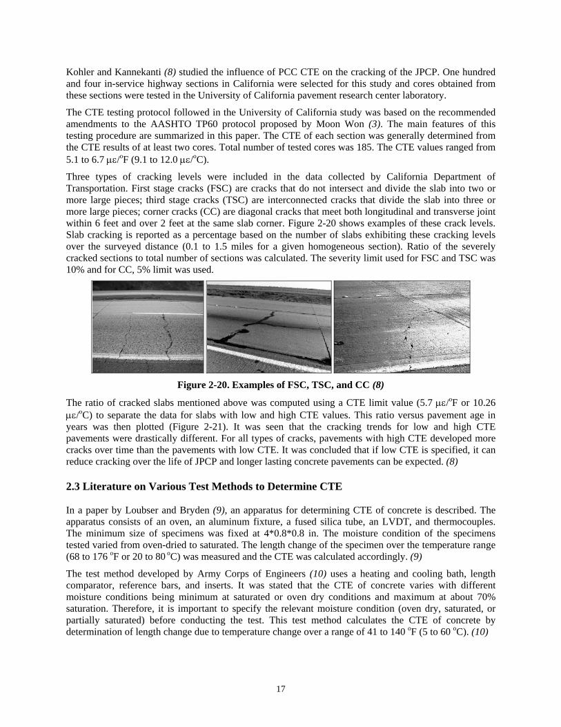
Kohler and Kannekanti (8) studied the influence of PCC CTE on the cracking of the JPCP. One hundred and n-service highway sections in California were selected for this study and cores obtained from thes e tested in the University of California pavement research center laboratory.

The CTE testing protocol followed in the University of California study was based on the recommended ame e AASHTO TP 0 protocol proposed by Moon Won (3). The main features of this testing procedure are summarized in this paper. The CTE of each section was generally determined from the CTE results of at least two cores. To was 185. The CTE values ranged from 5.1

Thr California Department of Tra t do not intersect and divide the slab into two or mor r onnected cracks that divide the slab into three or mor acks that meet both longitudinal and transverse joint with . igure 2-20 shows examples of these crack levels. Slab mber of slabs exhibiting these cracking levels ove ven homogeneous section). Ratio of the severely crac ated. The severity limit used for FSC and TSC was 10%

four ie sections wer

ndments to th 6

tal number of tested coresto 6.7 µε/oF (9.1 to 12.0 µε/oC).

ee types of cracking levels were included in the data collected bynsportation. First stage cracks (FSC) are cracks te large pieces; third stage cracks (TSC) are intee large pieces; corner cracks (CC) are diagonal cr

hac

in 6 feet and over 2 feet at the same slab corner cracking is reported as a percentage based on the nu

r the surveyed distance (0.1 to 1.5 miles for a giked sections to total number of sections was calcul and for CC, 5% limit was used.

F

Figure 2-20. Examples of SC, TSC, and CC (8)

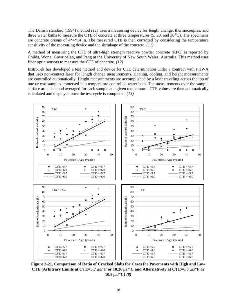
The omputed using a CTE limit value (5.7 µε/oF or 10.26 µε/o and high CTE values. This ratio versus pavement age in

ears was then plotted (Figure 2-21). It was seen that the cracking trends for low and high CTE

d longer lasting concrete pavements can be expected. (8)

ds to Determine CTE In a paper by Loubser and Bryden (9), an apparatus for determining CTE of concrete is described. The apparatus consists of an oven, an aluminum fixture, a fused silica tube, an LVDT, and thermocouples. The minimum size of specimens was fixed at 4*0.8*0.8 in. The moisture condition of the specimens tested varied from oven-dried to saturated. The length change of the specimen over the temperature range (68 to 176 oF or 20 to 80 oC) was measured and the CTE was calculated accordingly. (9)

The test method developed by Army Corps of Engineers (10) uses a heating and cooling bath, length comparator, reference bars, and inserts. It was stated that the CTE of concrete varies with different moisture conditions being minimum at saturated or oven dry conditions and maximum at about 70% saturation. Therefore, it is important to specify the relevant moisture condition (oven dry, saturated, or partially saturated) before conducting the test. This test method calculates the CTE of concrete by determination of length change due to temperature change over a range of 41 to 140 oF (5 to 60 oC). (10)

F

ratio of cracked slabs mentioned above was cC) to separate the data for slabs with low

ypavements were drastically different. For all types of cracks, pavements with high CTE developed more cracks over time than the pavements with low CTE. It was concluded that if low CTE is specified, it can reduce cracking over the life of JPCP an 2.3 Literature on Various Test Metho

17

18

imens re concrete prisms of 4*4*14 in. The measured CTE is then corrected by considering the temperature

g device and the shrinkage of the concrete. (11)

nder a contract with FHWA at uses non-contact laser for length change measurements. Heating, cooling, and height measurements

The Danish standard (1994) method (11) uses a measuring device for length change, thermocouples, and ree water baths to measure the CTE of concrete at three temperatures (5, 20, and 30 oC). The specth

asensitivity of the measurin

A method of measuring the CTE of ultra-high strength reactive powder concrete (RPC) is reported by Childs, Wong, Gowripalan, and Peng at the University of New South Wales, Australia. This method uses iber optic sensors to measure the CTE of concrete. (12) f

InstroTek has developed a test method and device for CTE determination uthare controlled automatically. Height measurements are accomplished by a laser traveling across the top of one or two samples immersed in a temperature controlled water bath. The measurements over the sample surface are taken and averaged for each sample at a given temperature. CTE values are then automatically calculated and displayed once the test cycle is completed. (13)

Figure 2-21. Comparison of Ratio of Cracked Slabs for Cases for Pavemen s with High and Low CTE (Arbitrary Lim E=6.0 µε/°F or

10.8 µε/°C) (8)

FSC90

0

R 10atio

20 of c

r 30ack 40

50

ed sl

60

abs

70

(k) .

80

0 10 2 30 40 50

Pavement Age (years)

0

CTE >5.7 CTE <=5.7CTE >6.0 CTE <=6.0CTE >5.7 CTE <=5.7CTE >6.0 CTE <=6.0

FSC+TSC

0

1020

30

4050

60

7080

90

0 10 20 30 4

Pavement Age (years)

Rat

io o

f cra

cked

slab

s (k)

.

0 50

TSC90

0 30 40 50

Pavement Age (years)

0

10Rat

io 20 of 30cr

ac

4050

ked

s60

lab

70

s (k)

.

80

0 10 2

CTE >5.7 CTE <=5.7CTE >6.0 CTE <=6.0CTE >5.7 CTE <=5.7CTE >6.0 CTE <=6.0

CTE >5.7 CTE <=5.7CTE >6.0 CTE <=6.0CTE >5.7 CTE <=5.7CTE >6.0 CTE <=6.0

CC

0

1020

30

4050

60

7080

90

0 10 20 3

Pavement Age (years

Rat

io o

f cra

cked

slab

s (k)

.

0 40 50

)

CTE >5.7 CTE <=5.7CTE >6.0 CTE <=6.0CTE >5.7 CTE <=5.7CTE >6.0 CTE <=6.0

tits at CTE=5.7 µε/°F or 10.26 µε/°C and Alternatively at CT

2.4 State-of-the-Practice Survey Results As part of the literature review, the authors also documented the process followed by various state DOTs. The survey instrument presented in Table 2-3 was sent to 50 state DOTs. Table A-1 of Appendix A summarizes the responses received from 17 state DOTs. Based on survey results, as of July 2006, only four states (AL, KS, TX, and UT) have initiated studies to document CTE for pavement design.

Ta urv nsUse this form t rtic a surve Coefficient of Thermal Expansion (CTE) practices currently used by State Highway Agencies in the United States. This survey is being conducted as part of a Michigan Department of Tran ta udy d “Quantif hermal Expansion Values of Typical Hydraulic Ce te Pa Mix

e

ble 2-3. S ey Io pa

trumipat

ent e in y of

spor tion stment Concre

Partic

titleving

ipant D

ying Coefficient of Ttures.”

tails N ame Title Organization Phone Number Fax Number Em ddre ail a ss

CTE Testing Practices Do our typical

c te pa mixtures? If yes, what testl do agen ollow?

you conduct CTE tests for yconpro

retoco

vinges your

cy f

Hoexaagg

w do you utilize your CTE information (for e, a input pavement design,te a tan "

mplrega

s anccep

intotc.)?

ce, e

Whaggsta

at are th pical l ogies of the coarse regate used in concrete paving mixtures on

te eral funded projects? Example lithologies are (but not limited to): ultramafic, g sc gneis mestone, dolomite,sandstone, slate, etc.

e ty ithol

/fed

ranite, hist, s, li

What are the typical CTE ranges for concrete mixtures containing the various coarse aggregate lithologies stated in the previous

n?

questioIn yothag

ourer c

grega

exp ce E testin hat omponents of the concrete m fine te, c nt, cem eplacements,etc)

have a significant impact on the test results?

erien

eme

with CT

ent r

g, wix (

Do you have any research results, either published or unpublished, that you could send or provide the location on your website?

Res(Pr

ponses req ed 2 . Please d the ple ey to Dr. Neeraj Buch i Inve ato email ress is h@eg u.ed

ueststig

by June 30,r).

006 add

sen comr.ms

ted u

survncipal The buc . Alter y the completed

v can be f to 0012.

nk you for participating in the survey.

nativelsur Tha

ey axed 517-432-

19

CHAPTER 3: DESCRIPTION OF THE EXPERIMENTAL PROGRAM

3.1 Introduct This chapter provides detail rials use e fabrication of the test specimens, the tests used for determining fresh propert nd the CTE test protocols. 3.2 Material d Hardened Concrete Properties Tests The concrete used in the fabr drical and prismatic test specimens was supplied by a local ready mix supplier. This ensured that all specimens needed for a given mixture were produced from a single batch, thereby reducing experiment variability. The coarse aggregate sources are presented in Table 3-1. Figure 3-1 show e variou egate sources within the state of Michigan. Mineralogical composition ies are summarized in Tables 3-2 through 3-4. Table 3-1. Coarse Aggregate Types and Source Name

Agg. Source, County

ion

s regarding the mate d in th and hardened concrete ies, a

s, Fresh an

ication of cylin

s the locations of than rt

s aggrd physical prope

s Mix ID Primary Agg. Class CTE 1 Limestone Pit # 71-47, Presque Isle CTE 2 Gravel Pit # 19-56, Clinton CTE 3 Limestone Pit # 75-5, Schoolcraft CTE Slag Pit # 8 4 2-19, Wayne CTE 5 Dolomite Pit # 49-65, Mackinac CTE 6 Gabbro Pit # 95-10, OntarioCTE 7 Dolomite Pit # 58-11, Monroe CTE Dolomite Pit # 91-06, 8 Cook

Figure 3-1. Locations of Some of the Aggregate Sources (After 14)

20

21

Table 3-2. Mineralogical and Physical Prope te (14) n % ig

rties of the CoMi

arse eral

Aggrega by We ht Mix

ID Primary

Rock Type C e her iption

ecifraviten D aCa-

Mg(CO3)2Ca O3 F S2 Ot

DescrSpG

Ov

ic y, ry

AbsCap

orption city

CTE 1 Limestone . . .54

Tan to brown, to dark brown abundant ossi fi 2.575 1.14 4.58 94 33 0 14 0 f

li

withn a e

ls imeston

ne gmatrix

rai

ned

CTE 2 Gravel * 2 .7N/A .571 2 0

CTE 3 Limestone .79 . 94 rai 9 0.69 7.27 90 0 06 0. Lg

ight taned

n tolim

tan festone

ine 2.64

CTE 4 Slag *

The vesicular particles are grey, the dense particles are grey to tan o wn,

e we

vitreous exposure

2 9 2.78 r broles ck

thy

glassy pllowish to

articbla

sho .32

CTE 5 Dolomite .48 Light tan to gray medium to coarse graine

lom5 .68 98.14 0 0.04 0.91 d

do ite 2.73 0

CTE 6 Gabbro **

bbr r pgio or

minor phases: mquartz and apatite

0 0.21

Gapla

o, majoclase, h

hasnbleagn

es: ndetit

e, e, 2.91

CTE 7 Dolomite .54 0.27 2.5 tan to gray fine to grained dolom 2.548 3.13 0 Light

medium ite 95.14 0

CTE 8 Dolomite N/A * Petrographic composition is reported in Table 3** Chemical composition is reported in Table 3-4

-3. .

Table 3-3. Petrographic Composition of Slag and Gravel Aggregates*

Mix ID Primary

Rock Aggregate Type Weight Mineral % by

Type Igneous/Metamorphic 54

Dense Carbonates 35.4 Absorbent Carbonates 4.7 Non-Friable Sandstone 1.0

Friable Sandstone 1.7 Siltstone 0.6

Shale + Coal 0.1 Clay Ironstone 0.5

CTE 2 Gravel

Chert 2 Vesicular Particles 85.7

Dense Particles 10.8 Glassy Particles 3.3 CTE 4 Slag

Magnetic Particles 0.2 * This information was provided by MDOT. Table 3-4. Chemical Composition of Gabbro Aggregate (14)

Mix ID Primary Rock Type Oxide/Element Oxide/Element % by

Weight MgO 8.44 Al2O3 18.61 SiO2 45.53

S 0.02 CaO 11.81

CTE 6 Gabbro

2 3Fe O 13.13 The typical concrete mixture d imens is summarized in Table 3-5.

Ingredients CTE 1 CTE 2 CTE 3 CTE 5 CTE 6 CTE 7 CTE 8a

esigns used in the fabrication of the test spec

Table 3-5. Concrete Mixture Designs (lbs/yd3)

CTE 4 Cement 564 564 560 560 560 573 560 376 Water 259 259 250 252 275 258 242 155 Coarse Agg. 1740 1760 1838 1575 1908 1774 1715 1942 Fine Agg. 1360 1360 1338 1348 1260 1230 1330 1444 AEA, (fl. oz.) 10 10 7.5 7.5 7.5 7.5 7.5 28 a This mixture design also included 94 lbs/yd3 of Fly Ash. Concrete specimens (except for CTE 8) were prepared at the MSU Civil Infrastructure Laboratory (CIL) according to the ASTM C 192 “Standard Practice for Making and Curing Concrete Test Specimens in the Laboratory”. CTE 8 specimens were field prepared specimens from an actual paving project in Michigan. At least three replicate samples were fabricated for each test. Over 700 specimens were fabricated to characterize the mechanical properties and CTE of the concrete paving mixtures. Thermocouples were embedded in the center of designated specimens to monitor concrete temperature for the CTE tests. All specimens were de-molded after 24 hours and were cured at 100% relative humidity and 23oC temperature in an environment chamber until the time of testing. CTE specimens were placed in a limewater bath as required by the test protocols. Once the specimens were de-molded and cured for an

22

appropriate time, various tests were conducted to assess the properties of interest. The material characterization tests performed on the concrete samples are summarized in Table 3-6.

Table 3-6. Summary of Material Characterization Tests

Test Attribute

Test Name/Equipment

ASTM Designation

Measured Property

No. of Specimens

Frequency of Testing

Slump C 143 Concrete workability

Air content C 231 Total air

content of fresh concrete

Unit weight C 138 Unit weight

Properties of Fresh Concrete

Temperature C 1064 Temperature

One per batch Not applicable

Compressive strength* C 39

Flexural strength C 78 Split tensile

strength C 496

Concrete strength

Properties of

Hardened Concrete

Elastic modulus C 469 Concrete stiffness

1, 3, 7, 14, 28, 90, 365 days

after specimen fabrication

Thermal Property

Coefficient of thermal expansion

AASHTO TP60

Linear length change/unit change in

Three replicates for each

test/batch 3, 7, 14, 28, 90,

180, 365 days after specimen

fabrication temperature * Compressive strengthmodulus of elasticity.

was determined by the same apparatus and specimen used to determine the

ansion of Hydraulic Cement Concrete”. The CTE test apparatus consists of a (i) temperature ontrolled water bath; (ii) rigid frame to support the est specimen; (iii) LVDT to record the change in

specimen length; and (iv) data ection. Figures 3-2a and 3-2b lustrate the CTE test setup.

Figure 3-2a. Schematic of the Test Setup

3.3 Thermal Property Test (Coefficient of Thermal Expansion Test) CTE test was conducted according to the AASHTO TP60 “Standard Test Method for the Coefficient of

hermal ExpTc t

acquisition system for continuous data collil

Controlled Temperature Water Bath Computer

Data Acquisition System

LVDT

Thermocouple

Fixture and Specimen

LVDT Power Supply

Invar Rod

23

Figure 3-2b. Complete Test Setup 3.3.1 Controlled Temperature Water Bath Three “PolyScience” Programmable Refrigerating/Heating Circulatorstemperature range for these circulators is -25 to +150°C with temperatushows a Model 9612 circulator.

Figure 3-3. Controlled Temperature Water

Computer Data Acquisition LVDT Power Supply

Temperature Con

24

Water Bath

r

B

LVDT

e Fixtur

were used in this experiment. The e stability of ±0.01 °C. Figure 3-3

ath

troller

Water Reservoir Lid

(15)

3.3.2 Data Acquisition System An “IOtech” Personal Daq/3000 data acquisition system was used to read and record the length changes of the specimens through LVDTs and record water bath temperatures. This system has eight analog inputs. The data acquisition system is shown in Figure 3-4.

Figure 3-4. Data Acquisition System (16)

The software used with this system was DaqView™ which allows the user to save the data in text format among other file formats. A screen shot of the channel setup is illustrated in Figure 3-5.

Figure 3-5. DaqView™ annel Setup Screen Software Ch

25

3.3.3 Linear Variable Differential Transformer (LVDT)

D 750-050 Spring-Loaded DC-LVDT Position Sensors were used to measure the length changes of concrete specimens subjected to temperature cycles. These LVDTs have a nominal range of ±0.050 in. from null position and full scale output of 0 to ±10 V DC. Figure 3-6 shows the LVDTs.

Three “Macro Sensors” GHS

Figure 3-6. Spring-Loaded LVDTs (17)

3.3.4 Rigid Support Frame Rigid support frames were fabricated based on AASHTO TP60 appendix X.1 “Specimen Measuring Apparatus”. Figure 3-7 shows the rigid support frame. The circular base plate is made of Aluminum and has a diameter of 10 inches. Three semi-spherical support buttons equally spaced around a 2 inch diameter circle are placed on the base plate. The frame height is 10 inches and the vertical rods are made of Invar (a nickel-iron alloy with very low CTE) in order to minimize the effect of frame length changes on the measurements. The side view and plan view of the rigid support frame are shown in Figure 3-8.

Semi-Spherical Supports

Figure 3-7. Rigid Support Frame

26

Invar Vertical Rods

Base Plate

s

S

F 3.3.5 Test Pr Specimens wenot suitable m ent, calculations.

o

isalignm

-0.0010

0005

00

0030

0035

-0.

0. 00

0.0005

0.0010

0.0015

0.0020

Dis

plac

emen

t (In

.)

0.0025

0.

0.

Invar Vertical Rod

Base Plate

emi-Spherical Supports

igure 3-8. Side View and Plan View of the Rigid Support Frame (After 18)

re subjected to at least three heating-coolin cles (Figure 3-9). e cy as for ations due oblem h test tionslack of proper seating of the specimen, etc.), the re cycles could be used for CTE

cedure and Data Collection

g cy This way, if on ( n and LVDT

cle wCTE calcul to pr s wit condi specime

plicate

0 200 400 600 1000 1200 1400

Time (Min

Figure 3-9. Three Typical Heating-Cooling Cycles

800

.)

27

A thermocouple was inserted in each bath to record the water temperature. Thermocouples were also mbedded in the concrete samples to monitor the specimen temperature during the CTE test. It was found

he Texas DOT method is shown in Figure 3-11.

ethat both the specimen and water follow similar temperature signature, however, the concrete specimen lags the water temperature by approximately 10 minutes. Figure 3.10 shows a typical temperature graph. Temperature and displacement were recorded at 1 minute intervals. The data collected this way was used to calculate CTE based on AASHTO TP60 procedure as well as the Texas DOT modified test procedure. A typical graph showing t

50.00

60.00

0.000

10.00

20.00

50 150 00 250 300

Time (min

30.00

mpe

ratu

r

40.00

e (°

C)

100 2

)

Te

Concrete Temp. W Temp.ater

0.000

50.00

60.00

50.00

60.00

40.00

10.00

20.00

30.00

0.000

10.00

20.00

50 150 00 250 300

Time (min

30.00

mpe

ratu

r

40.00

e (°

C)

Te

100 2

)

Concrete Temp. W Temp.

A Typical Concrete and Water Temperature G

ater

Figure 3-10. raph

-0.00100

-0.00050

0.00000

0.00050

0.00100

0.00150

0.00200

0.00

5.00 10.00 15.00 20.00 25.00 30.00 35.00 40.00 45.00 50.00

Temperature (°C)

Dis

plac

emen

t (in

.)

250Heating-S Cooling-S Linear (Heating-S) Linear (Cooling-S

Figure 3-11. A Typical Texas DOT Method Graph

)

28

3.3.6 CTE Calculations Based on the sample temperature and displacements the following computational sequence is followed to establish CTE value. The CTE test result is the average of heating and cooling cycle CTE values providing that the difference between the values does not exceed 0.5 µε/°F (0.3 µε/°C).

CTE = (CTEHEATING + CTECOOLING) / 2 CTE of the heating or cooling cycle is defined as the actual length change of the specimen (∆LACTUAL) divided by the initial length of the specimen (LINITIAL) over the temperature range (∆T).

CTE HEATING or COOLING = (∆LACTUAL / LINITIAL) / ∆T

The actual length change is defined as the summation of the measured length change of the specimen (∆LSPECIMEN) and the length change of the measuring apparatus (∆LAPPARATUS).

∆LACTUAL = ∆LSPECIMEN + ∆LAPPARATUS The length change of the measuring apparatus is the product of the correction factor of the measuring apparatus (Cf), initial length of the specimen (LINITIAL), and the temperature range (∆T).

The correction factor of the measu Appendix X.2 of the AASHTO TP60 standard. (18)

∆LAPPARATUS = Cf × LINITIAL × ∆T

ring apparatus is obtained according to

29

CHAPTER 4: RESULTS AND DISCUSSION 4.1 Introduction This chapter documents the results of the laboratory experimental program described in Chapter 3. The results summarized in this chapter include (i) physical properties of aggregates; (ii) fresh and hardened properties of the concrete; and (iii) coefficient of thermal expansion of concrete made from various aggregate rock types. Furthermore, the statistical and operational significance of test variables on the magnitude of CTE are presented in this chapter. The structural design implications of CTE are also summarized as part of this chapter. 4.2 Physical Properties of Coarse Aggregates The absorption capacity and specific gravity tests (ASTM C127) were conducted on sampled aggregates. For each aggregate type, the sample was divided into four batches and tests were conducted on each batch. The results were then averaged. The summarized results are presented in Table 4-1. Table 4-1. Physical Properties of Coarse Aggregates

Specific Gravity Mix ID Primary Aggregate Class Pit

Number

Absorption Capacity,

% Apparent Bulk Saturated Surface-Dry

Bulk Dry

CTE 1 Limeston 2.591 2.552 e 71-47 1.13 2.655 CTE 2 Gravel 2.637 2.566 19-56 2.77 2.762 CTE 3 Dolomitic Limeston 2.668 2.649 e 75-05 0.69 2.698CTE 4 Slag 2.393 2.329 82-19 3.47 2.490 CTE 5 Dolomite 49-65 0.68 2.787 2.753 2.735 CTE 6 Gabbro (Trap Rock) 95-10 0.21 2.928 2.916 2.910 CTE 7 Dolomite 58-11 3.13 2.769 2.628 2.548

4.3 Fresh Concrete Properties Fresh concrete properties results conducted according to aforementioned standards (Table 3.6) are shown in Table 4-2. The target slump was 3 ± 0.5 in. and the target air content was 6.5 ± 1.5 %. It should be mentioned that these tests were conducted to make sure that the concrete tested in laboratory is not significantly different from the concrete used in field for paving. However, strict conformance to field parameters was not the goal of this study. Table 4-2. Fresh Concrete Properties

Test Parameter Mix ID Slump, inches Air, % Unit Weight, pcf Temperature, °FCTE 1 3.0 6.0 147.0 54 CTE 2 4.0 5.2 149.4 70 CTE 3 6.0 6.0 145.0 70 CTE 4 3.0 5.8 145.4 77 CTE 5 3.8 4.2 150.8 75 CTE 6 4.0 5.0 152.0 61 CTE 7 3.0 4.9 148.2 69

30

4.4 Hardened Concrete Properties Hardened concrete properties tests were conducted on laboratory cured specimens at 1, 3, 7, 14, 28, 90, and 365 days after casting. Results are summarized in Figures 4-1 through 4-31. The data used for developing the summary tables and graphs are presented in Appendix B. Dashed lines in the plots represent the target 28-day compressive and flexural strength as suggested by MDOT. Three replicate specimens were tested at each specified age. The error bars represent the standard deviation of test values among three replicates. All concrete batches conformed to 28-day compressive strength of 3500 psi. Except for mix IDs 2 and 3, the flexural strength requirement of 720 psi was met. However, both of these mixes met the requirement at 90 days of age. The impact of this minor non-conformance on CTE is not going to be significant in the author’s opinion. The hardened concrete property tests were conducted for two reasons:

• To evaluate the quality of the concrete • To be used as level 1 inputs in M-E PDG and HIPERPAV II software

In general, the delivered concrete met the required specified strengths. Table 4-3 presents the average 28-day hardened concrete properties. Table 4-3. Average 28-Day Strength Properties (psi)

Test Parameter Mix ID Compressive

Strength Split Tensile

Strength Flexural Strength

Elastic Modulus (*10-6)

CTE 1 5129 516 836 4.50 CTE 2 4965 4.89 502 692 CTE 3 3967 4.57 489 645 CTE 4 5169 4.66 507 831 CTE 5 4035 511 731 4.65 CTE 6 5125 500 731 5.39 CTE 7 5825 561 820 4.48 CTE 8 4953 489 N/A 4.71

31

0500

1000150020002500300035004000450050005500600065007000

1 3 7 14 28 90 365

Time, days

Com

pres

sive

stre

ngth

, psi

Sample 1 Sample 2 Sample 3 28-day target

Figure 4-1. CTE 1 Compressive Strength

0.0

1.0

2.0

3.0

4.0

5.0

6.0

1 3 7 14 28 90 365

Time, days

Ela

stic

mod

ulus

x 1

06 , psi

Sample 1 Sample 2 Sample 3

Figure 4-2. CTE 1 Elastic Modulus

32

0

100

200

300

400

500

600

700

1 3 7 14 28 90 365

Time, days

Split

tens

ile st

reng

th, p

si

Sample 1 Sample 2 Sample 3

Figure 4-3. CTE 1 Splitting Tensile Strength

0

120

240

360

480

600

720

840

960

1 3 7 14 28 90 365

Time, days

Flex

ural

stre

ngth

, psi

Sample 1 Sample 2 Sample 3 28-day target

Figure 4-4. CTE 1 Flexural Strength

33

0500

100015002000250030003500400045005000550060006500

1 3 7 14 28 90 365

Time, days

Com

pres

sive

stre

ngth

, psi

Sample 1 Sample 2 Sample 3 28-day target

Figure 4-5. CTE 2 Compressive Strength

0.00

1.00

2.00

3.00

4.00

5.00

6.00

1 3 7 14 28 90 365

Time, days

Ela

stic

mod

ulus

x 1

06 , psi

Sample 1 Sample 2 Sample 3

Figure 4-6. CTE 2 Elastic Modulus

34

0

100

200

300

400

500

600

700

1 3 7 14 28 90 365

Time, days

Split

tens

ile st

reng

th, p

si

Sample 1 Sample 2 Sample 3

F igure 4-7. CTE 2 Splitting Tensile Strength

0

120

240

360

480

600

720

840

960

1 3 7 14 28 90 365

Time, days

Flex

ural

stre

ngth

, psi

Sample 1 Sample 2 Sample 3 28-day target

Figure 4-8. CTE 2 Flexural Strength

35

0500

10001500200025003000350040004500500055006000

1 3 7 14 28 90 365

Time, days

Com

pres

sive

stre

ngth

, psi

Sample 1 Sample 2 Sample 3 28-day target

Figure 4-9. CTE 3 Compressive Strength

0.00

1.00

2.00

3.00

4.00

5.00

6.00

1 3 7 14 28 90 365

Time, days

Ela

stic

mod

ulus

x 1

06 , psi

Sample 1 Sample 2 Sample 3

Figure 4-10. CTE 3 Elastic Modulus

36

0

100

200

300

400

500

600

700

1 3 7 14 28 90 365

Time, days

Split

tens

ile st

reng

th, p

si

Sample 1 Sample 2 Sample 3

F igure 4-11. CTE 3 Splitting Tensile Strength

0

120

240

360

480

600

720

840

960

1 3 7 14 28 90 365

Time, days

Flex

ural

stre

ngth

, psi

Sample 1 Sample 2 Sample 3 28-day target

Figure 4-12. CTE 3 Flexural Strength

37

0500

10001500200025003000350040004500500055006000650070007500

1 3 7 14 28 90 365

Time, days

Com

pres

sive

stre

ngth

, psi

Sample 1 Sample 2 Sample 3 28-day target

Figure 4-13. CTE 4 Compressive Strength

0.00

1.00

2.00

3.00

4.00

5.00

6.00

1 3 7 14 28 90 365

Time, days

Ela

stic

mod

ulus

x 1

06 , psi

Sample 1 Sample 2 Sample 3

Figure 4-14. CTE 4 Elastic Modulus

38

0

100

200

300

400

500

600

700

1 3 7 14 28 90 365

Time, days

Split

tens

ile st

reng

th, p

si

Sample 1 Sample 2 Sample 3

F igure 4-15. CTE 4 Splitting Tensile Strength

0

120

240

360

480

600

720

840

960

1 3 7 14 28 90 365

Time, days

Flex

ural

stre

ngth

, psi

Sample 1 Sample 2 Sample 3 28-day target

Figure 4-16. CTE 4 Flexural Strength

39

0500

100015002000250030003500400045005000550060006500

1 3 7 14 28 90 365

Time, days

Com

pres

sive

stre

ngth

, psi

Sample 1 Sample 2 Sample 3 28-day target

Figure 4-17. CTE 5 Compressive Strength

0.00

1.00

2.00

3.00

4.00

5.00

6.00

7.00

1 3 7 14 28 90 365

Time, days

Ela

stic

mod

ulus

x 1

06 , psi

Sample 1 Sample 2 Sample 3

Figure 4-18. CTE 5 Elastic Modulus

40

0

100

200

300

400

500

600

700

1 3 7 14 28 90 365

Time, days

Split

tens

ile st

reng

th, p

si

Sample 1 Sample 2 Sample 3

F igure 4-19. CTE 5 Splitting Tensile Strength

0

120

240

360

480

600

720

840

960

1 3 7 14 28 90 365

Time, days

Flex

ural

stre

ngth

, psi

Sample 1 Sample 2 Sample 3 28-day target

Figure 4-20. CTE 5 Flexural Strength

41

0500

10001500200025003000350040004500500055006000

1 3 7 14 28 90 365

Time, days

Com

pres

sive

stre

ngth

, psi

Sample 1 Sample 2 Sample 3 28-day target

Figure 4-21. CTE 6 Compressive Strength

0.00

1.00

2.00

3.00

4.00

5.00

6.00

7.00

1 3 7 14 28 90 365

Time, days

Ela

stic

mod

ulus

x 1

06 , psi

Sample 1 Sample 2 Sample 3

Figure 4-22. CTE 6 Elastic Modulus

42

0

100

200

300

400

500

600

700

1 3 7 14 28 90 365

Time, days

Split

tens

ile st

reng

th, p

si

Sample 1 Sample 2 Sample 3

F igure 4-23. CTE 6 Splitting Tensile Strength

0

120

240

360

480

600

720

840

960

1 3 7 14 28 90 365

Time, days

Flex

ural

stre

ngth

, psi

Sample 1 Sample 2 Sample 3 28-day target

Figure 4-24. CTE 6 Flexural Strength

43

0500

10001500200025003000350040004500500055006000650070007500

1 3 7 14 28 90 365

Time, days

Com

pres

sive

stre

ngth

, psi

Sample 1 Sample 2 Sample 3 28-day target

Figure 4-25. CTE 7 Compressive Strength

1.00

6.00

E x

10 4.006 , p

s

5.00i

2.00

3.00

last

ic m

odul

us

0.001 3 7 14 28 90 365

Time, days

Sample 1 Sample 2 Sample 3

Figure 4-26. CTE 7 Elastic Modulus

44

0

100

200

300

400

500

600

700

1 3 7 14 28 90 365

Time, days

Split

tens

ile st

reng

th, p

si

Sample 1 Sample 2 Sample 3

Figure 4-27. CTE 7 Splitting Tensile Strength

0

120

240

360

480

600

720

840

960

1 3 7 14 28 90 365

Time, days

Flex

ural

stre

ngth

, psi

Sample 1 Sample 2 Sample 3 28-day target

Figure 4-28. CTE 7 Flexural Strength

45

0500

1000150020002500300035004000450050005500600065007000

7 14 28 90 365

Time, days

Com

pres

sive

stre

ngth

, psi

Sample 1 Sample 2 28-day target

Figure 4-29. CTE 8 Compressive Strength*

0.00

1.00

2.00

3.00

4.00

5.00

6.00

7 14 28 90 365

Time, days

Ela

stic

mod

ulus

x 1

06 , psi

Sample 1 Sample 2

Figure 4-30. CTE 8 Elastic Modulus*

46

0

100

200

300

400

500

600

700

7 14 28 90 365

Time, days

Split

tens

ile st

reng

th, p

si

Sample 1

For CTE 8,

compressive strength and elastic modulus test, and the other specimen was

for concretes made with that r Mechanistic-Empirical Design” 1-37A (19) which are shown in

Figure 4-31. CTE 8 Splitting Tensile Strength*

* there were a total of three specimens for each test age. After CTE test was conducted, two of the specimens were used for

sed for splitting tensile test. u 4.5 Thermal Properties The CTE test was conducted on laboratory cured specimens at 3, 7, 14, 28, 90, 180, and 365 days after casting. CTE was calculated based on both AASHTO TP60 and Texas DOT 428 A methods. The results are presented in Figures 4-32 through 4-39. The data used for computing the summary information are presented in Appendix C. The error bars in these figures show the standard deviation of the test specimens

ased on three replicates. The dashed lines show the typical CTE rangesbparticular aggregate based on “Guide fo

able 4-4. T The average 28 day CTE values of concrete samples made with limestone (CTE 1,3) were 4.54 and 4.51 µε/°F (8.18 and 8.11 µε/°C). For concrete made with dolomite coarse aggregate (CTE 5, 7, and 8) the average 28 day values ranged from 5.87 to 5.92 µε/°F (10.57 to 10.65 µε/°C). For concrete samples made with gravel aggregate (CTE 2), this value was 5.84 µε/°F (10.52 µε/°C). The value for concrete made with slag (CTE 4) was 5.71 µε/°F (10.27 µε/°C). The average 28 day CTE value obtained for concrete made with gabbro (trap rock) was 5.41 µε/°F (9.73 µε/°C).

47

Table 4-4. Typical CTE Ranges for Common Components and Concrete (19)

4.5

5.5

6.5

7.5

8.5

CT

9.5

10.5

µε/

°

11.5

12.5

13.5

3 7 14 28 90 180 365

E,

2.5

3.5

6.5

7.5

, µ

C 5.5 ε/°F

4.5 CT

E

Time, days

AASHTO TP 60 TxDOT 428-A Minimum Maximum

F igure 4-32. CTE 1 (Limestone Concrete) Coefficient of Thermal Expansion

48

4.55.56.57.58.59.5

10.511.512.513.514.515.516.5

3 7 4 90 180 365Ti , day

CT

ε/°

17.5 9.5

1 28me s

E, µ

C

2.5

3.5

4.5

5.5

6.5

8.5

7.5

CT

E, µε/

°F

AASHT 60O TP TxDO 28-AT 4 Minimum Maxim

Figure 4-33 TE 2 (Gra ) C icien f The al E nsion

um

. C vel Concrete oeff t o rm xpa

4.53 7 14

5.5

9.5

10.5

11.5

12.5

13.5

28 90 180 365

ε 5.5

6.5

7.5

6.5

7.5

8.5E, µ

/°C

CT

E, µε/

°F

CT 4.5

3.5

2.5

Time, days

AASHTO TP 60 TxDOT 428-A Minimum Maximum

Figure 4-34. CTE 3 (Dolomitic Limestone Concrete) Coefficient of Thermal Expansion

49

4.5

5.5

6.5

7.5

8.5

9.5

10.5

11.5

12.5

13.5 7.5

3 7 14 28 90 180 365Time, days

CT

E, µε/

°C

2.5

3.5

4.5

5.5

6.5

CT

E, µε/

°F

AASHTO TP60 TxDOT 428-A Minimum Maximum

Figure 4-35. CTE 4 (Slag Concrete) Coefficient of Thermal Expansion

4.5

5.5

6.5

7.5

8.5

9.5

CT

E, µε/

°

10.5

11.5

12.5

13.5

s3 7 14 28 90 180 365

Time, day

C

2.5

3.5

4.5

5.5C

TE

, µε/

°

6.5

7.5

F

AASHTO TP60 TxDOT 4 -A28 Minimum Maximum

Fig on ure 4-36. CTE 5 (Dolomite Concrete) Coefficient of Thermal Expansi

50

7.513.5

4.5

5.5

.5

9.5

12.5

90 180 365Time, days

µε

6.5

7

10.5

11.5/°

8.5

CT

E,

C

2.5

3.5

4.5

5.5

CT

E, µε/

°

6.5

3 7 14 28

F

AASHTO TP-60 TxDOT 428-A Minimum Maximum

Figure 4-37. CTE 6 (Gabbro or Trap Rock Concrete) Coefficient of Thermal Expansion

4.5

7.513.5

12.5

2.5

6.511.5

5.5

6.5

7.5

CT 8.5

9.5

10.5

E, µε/

°C

3 7 14 28 90 180 365Time, days

3.5

4.5

5.5C

TE

, µε/

°F

AASHTO TP60 TxDOT 428-A Minimum Maximum

Figure 4-38. CTE 7 (Dolomite Concrete) Coefficient of Thermal Expansion

51

4.5

5.5

6.5

2.5

3.5

7.5

ε

7.5

8.5

CT

E, µ

9.5

13.5

7 14 28 90 180 365Time, days

ε

10.5

11.5

12.5/°C 5.5

6.5

/°F

4.5 CT

E, µ

AASHTO TP60 TxDOT 428-A Minimum Maximum

Figure 4-39. CTE 8 (Dolomite Concrete) Coefficient of Thermal Expansion 4.6 CTE Test Variability The test variability (δCTE) was determined by subtracting the measured CTE within a batch (i.e. for a given mix ID and sample age) from the batch mean. Figure 4-40 illustrates the frequency histogram of δCTE. Approximately 98% of the data set has a δCTE between ± 0.3 µε/oF (0.5 µε/oC). The coefficient of variation ranges between 2.5% and 6%.The variability stems from a variety of factors including; (i) variable internal relative humidity in the sample at the time of testing; (ii) non-uniform temperature distribution in the sample; (iii) inhomogeneities in the specimen at the time of fabrication; (iv) LVDT sensitivity; (v) power fluctuations; and (vi) possible frame induced errors. 4.7 The factors that potentially affected the magni E in this experiment were aggregate geology, sample age, and number of heating-cooling cycles. To investigate the impact of these factors and their

eatmeexample sample age and number of heating-coolin gories called

esign

plicate samples for each

Statistical Analysis Approach

tude of the CT

interactions on the magnitude of CTE, a “factorial treatment design” was employed. In a factorial tr nt design, one factor, for example aggregate type, is tested over one or more other factors, for

g cycles. Each factor has several cate“levels”. For example, levels of the sample age factor are 3, 7, 14, 28, 90, 180, and 365 days. The dfactorial included, (i) aggregate geology with eight levels; (ii) sample age with seven levels and (iii)

umber of heating-cooling cycles with three levels. There were three rencombination of aggregate geology and sample age. Table 4-5 shows the factorial design table. Aggregate geology, sample age, and number of cycles were considered as fixed effects. In fixed effects, different levels of factors are reproducible. In other words if the experiment was to be repeated, the levels could be duplicated. Individual sample ID (replications) within each aggregate geology and sample age

52

1 0 2 38

14 15 13

52 0 1

0

10

25

3135 37

30

40

50

Freq

uenc

y

55 54

63

2120

77

70

80

90-0.5 µε/°C 0.5 µε/°C

60

-0.7

8

-0.7

0

-0.6

3

-0.5

5

-0.4

8

-0.4

0

-0.3

3

-0.2

5

-0.1

7

-0.1

0

-0.0

2

0.05

0.13

0.20

0.28

0.35

0.43

0.50

0.58

0.66

0.73

δCTE, µε/°C Figure 4-40. Variability Histogram

was considered as a random effect because for each combination of aggregate type and sample age, a sample ID was assigned randomly to the three replicates from the same batch of concrete. Additionally,

e number of cycles were treated as repeated measurements of individual samples since multiple easurements (cycles) were taken on each of the replicate samples.

ince the experiment included both fixed and random effects, the statistical analysis was performed using e “mixed effect” models. The following general linear model describes the relationships between ctors. The statistical significance of the factors and their interactions was evaluated by using the

nalysis of variance (ANOVA) method. (20)

= µ + Agg_Type + Age + Agg_Type*Age + Sample_ID(Agg_Type Age) + Cycle + Agg_Type*Cycle + ge*Cycle + Agg_Type*Age*Cycle + e

here: y = response variable which is the CTE value µ = overall mean

Agg_Type = fixed effect of the aggregate geology Age = fixed effect of the sample age at the time of testing

gregate geology and sample age Sample_ID(Agg_Type Age) = random effect of the replications

Cycle = fixed effect of the cycle numg_Type*Cy fect of the a gy and cycle

Age*Cy fect of the s cycle numberAgg_Type*Age*Cy t of th , sample age, and cycle numbers

ental e

thm Sthfaa yA w

Agg_Type*Age = interaction effect of the ag

bers Ag cle = interaction ef

cle = interaction efggregate geoloample age and

numbers s

cle = interaction effece = random experim

e aggregate geologyrror

53

Table 4-5. Factorial D

esign Table*

Age, DaysAggregate Geology

Nu bHeat -

Cycles 3 7 14 28 90 180 365 Total

m er of ing Cooling

1 X X X X X X X 7 2 X X X X X X X 7 CTE 1 3 X X X X X X X 7 1 X X X X X X X 7 2 X X X X X X X 7 CTE 2 3 X X X X X X X 7 1 X X X X X X X 7 2 X X X X X X X 7 CTE 3 3 X X X X X X X 7 1 X X X X X X X 7 2 X X X X X X X 7 CTE 4 3 X X X X X X X 7 1 X X X X X X X 7 2 X X X X X X X 7 CTE 5 3 X X X X X X X 7 1 X X X X X X X 7 2 X X X X X X X 7 CTE 6 3 X X X X X X X 7 1 X X X X X X X 7 2 X X X X X X X 7 CTE 7 3 X X X X X X X 7 1 N/A X X X X X X 6 2 N/A X X X X X X 6 CTE 8 3 N/A X X X X X X 6

Total 21 24 24 24 24 24 24 165 *Three replicates for each combination o considf factors were

ered tota e CTE values 65=49

The first step in the analys ass for el. ss rethe residuals (difference between predict easu s) to ) independen norm

ut and (iii) having a common variance for all levels of each factor.

T inde nde a p wa alu n by w h the vidu les wchosen for testing. This assumption was satisfied becau ples were randomly selected for CTE

nt ac gr e t nd

The normality um n ch d b n o butio the r als am) al probability plot of the residuals after eliminatio outliers. The residual histogram should

how a symmetric bell shaped distribution. The normal probability plot of the residuals should not deviate ignificantly from the straight line showed on the graph. Unusually high or low residuals were checked to

determine whether those residuals were outliers or not. Raw data (measurements) of such residuals were checked to detect any equipment malfunction during that particular test cycle. The histogram and normal probability plot of the residuals for the entire dataset are illustrated in Figures 4-41 and 4-42 respectively.

ling th the mod

be (i

to 3*1 umptions

t, (ii)

5 quire

ally

is requires the checking of

umptions

The a

ed and m red valuedistrib

he

ed,

pe nce ssum tion s ev ated based o the method e the sa

hic indi al samp ere s m

measure

me for e h ag egat ype a age.

ass ptio was ecke y inspectio f the distrin of the

n of esidu (histogr and normss

54

Figure 4-41. Histogram of the Residuals

Figure 4-42. Normal Probability Plot of the Residuals

55

The homogeneity of the variances was assessed by examination of the variances of the residuals for all levels of each factor. Side-by-side box plots were employed to help in the identification of the largest and smallest variances. For this assumption to be valid, the ratio of the largest variance to the smallest variance should not exceed 3, 5, or 10. These limits are different rules of thumb and “5” was selected for this analysis. Side-by-side box plots of the residuals for different levels of “age” variable are shown in Figure 4-43. In this figure the median is represented by the horizontal line inside the box. The top and bottom of the box represent the 3rd quartile (75th percentile) and the 1st quartile (25th percentile), respectively. The distance between these two is the interquartile range (IQR). Whiskers are drawn to capture the minimum and maximum observations. Based on the availability of the data for different comparisons and analyses, several datasets were used throughout the statistical analysis. For each dataset, the assumptions were checked and appropriate adjustments were made to the analyses where necessary.

Figure 4-43. Side-By-Side Box Plots of the Residuals for Age Factor

After checking the assumptions, the significance of the factors, and their interactions were investigated. The Least Significant Difference ( ethod was used for all-pairwise comparison f 0.05. A main or interaction effect was considered significant if the p-value was less th The results from the mixed effec summarized in Table 4-6. The i geology, sample age and num o cles on CTE is significant (P value less than 0.05). Furthermore, the interactions between (i) aggregate geology and sample age; and (ii y and number of heating-cooling c be statistically

LSD) m s with an α value oan 0.05.

ts analysis are mpact of aggregateber f heating-cooling cy

) aggregate geolog cy les were found to significant.

56

Table 4-6. Tests of Fixed Eff s Effect alue P Value

ectF V

Aggregate Type 383.73 <.0001 Age 33 <.0001 Aggregate Type*Age 1.57 0.0338 Cycle Number 123.09 <.0001 Aggregate Type*Cycle Numb er 5.47 <.0001 Age*Cycle Num 624 ber 1.42 0.1Aggregate Type*Age*Cycle Num 3 ber 1.14 0.30

4.7.1 Aggregate Type Effect Based gregate p n with age umber are significant (p-values

e vestigated for each level of age and cycle number factors. This implies that concrete samples made with

regate type nd sample age was examined. This implies that the effect of age on CTE was investigated within each

pared to all other levels (showed

geologies, different column bars having the same lette roup ch are a colum s to either one of t oth g T the impact o age within an a te type, an irwise pa u them as use nalysis, it was found that fo pes the magnitude of CTE at the end of 28 da s significantly different (lower) fro agnitu ee to 365 days 4 ber of Heating-Cooling Cycles Effe

sample from each CTE mix design was subjected to three heating and cooling cycles to study the effect ource, the heating and

cooling effect could be analyzed regatcooling cy ustr Figu . W n bars (repres vera E) as the s e le are t significantly different from each other at

nce el of 95 e sam ussio gar g the tters als

In most case xcept E 6) E m at en h s y ferent ) tha CTE er d e f -

ycle This c n w d on re fro r method. The ef e

on Table 4-6, ag ty e and its interactio and cycle nless than 0.05). Therefore, the effect of aggregate type (or geology) on the magnitude of CTE must bindifferent types of coarse aggregate (different geologies) have different CTE values. This finding is in agreement with the results of other research (References 1, 2, 3, and 7). 4.7.2 Sample Age Effect To investigate the effect of sample age at the time of test on CTE, the interaction effect of aggaaggregate type. The variation in CTE as a function of sample age for all aggregate types is illustrated in Figure 4-43. Within each aggregate type shown in Figure 4-44 the column bars (representing average CTE) assigned the same letter are not significantly different from each other at a confidence level of 95%. Some column bars have two letters assigned to them. In the all-pairwise comparison, each level of age is compared to all other levels. For example, in CTE 1, 3-day CTE was comby letter “a”). When 3-day CTE is different from 90-day CTE, this comparison is finished and a new comparison starts with 7-day CTE (denoted by letter “b”). Within each of the aggregate

r indicate a ghe groups,

of ages whibut not b

statistically similar. Ifn bar has two letters, it belong roups.

o study f sample ggrega all-pa com rison sing LSD ethod w d. Based on the LSD a r most aggregate ty

ys wa m the m de of CTE m asured at the nd of 90 .

.7.3 Num ct

Aon CTE. In addition, since each mix design was using a different coarse aggregate s

by aggre 4-45

e type. The variability in CTE as a function of heating-n each aggregate type shown in Figure 4-45 the columcles is ill

en g aated in ithi

tin ge CT signed am tter noa confide

lev %. Th e disc n re din le is o applicable to this analysis.

s (e for CT the CT deter ined the d of t e first heating-cooling cycle i the second and third heatingwise comparison using the LSD

significantlcooling c

dif (highero io

n the as base

det mine at th end os. same effect was observed in another stu

nclus the sults dy (R

m anerenc

all-pai 7).

57

5.5

6.5

9.5

11.5

12.5

13.5ve

rag

TE

, µ

4.5

5

erag

e C

7.5A

8.5e C

10.5

ε/°C

3.5

5.5 , µε/

°F

6.5

7.

Av

TE

aaaaa

bab

a a

a b a

d

a a

c

a b a

c

b

cb

aa

cc

aa abaa

d d d c b

cb

c c

b b c c

b a a

b bb aa

d d c b b

d c

d c

aaaaaa a a a

4.5CTE 1 CTE 2 CTE 3 CTE 4 CTE 5 CTE 6 CTE 7 CTE 8

Mix ID

2.5

3 7 14 28 90 180 365 Figure 4-44. Average CTE for Various Aggregates as a Function of Test Specimen Age Based on 3

Replicates *

8.0

8.5

11.5

9.0

9.5

Ave

rage

CT

E 10.0

.5

1 C C TE Cx

,

5.9

6.2

10

b a b b a b11.0

CTE CTE 2 TE 3 TE 4 C 5 TE 6 CTE 7 CTE 84.4

Mi ID

µε/

°C

4.7

5.0

5.3A

vera

ge C

TE

5.6

, µε/

°F

Cycle 1 Cycle 2 C 3

c

a

a

a a

b a b

Average CTE for Various Aggregates as a Function of Number of Cycles Based

on ep es

n s follo y the tter within a CTE m typ e n

b a b

b b

a

b a

b b

ycle

Figure 4-45. 3 R licat *

*The colum bar wed b same le ix e ar ot significantly different.

58

4.8 Impact TE o form Concrete Pa e Sensitivity a ses we ducte vest te t pact of C on )

sing ERPA and -te fe sin e N l Pavement De Guid E PD war th fo ce i P).

TE affects both thermally induced stresses within the pavement and joint movement. As a result,

of the data ynthesis is summarized in Table 4-8 and Figures 4-46 and 4-47. Since the HIPERPAV II analysis was

gure 4-47). In general avements made with these approved mix designs did not show any practical sensitivity to the magnitude

of C n Per ance of Jointed vem nts

naly re con d to in iga he im TE the short-term (first 72-hoursP 1-37A Mechanistic-Empiricanted concrete pavements (JC

effects u HIP V II, the long rm ef cts u g th CHRsign e (M- G) soft e on e per rman of jo

Cpremature cracking, mid panel and corner cracking, faulting, and joint spalling can occur as mentioned. In order to minimize the occurrence of these distresses, the CTE value among other variables must be considered while designing a pavement. The performance parameter of interest for the short term effect was ratio of the maximum stress in concrete slab to PCC strength. The performance parameter of interest for the long term effect was transverse cracking. Tables 4-7 and 4-9 summarize the sensitivity matrices used to investigate the short and long-term effects of CTE on the performance of JCPs. 4.8.1 Short Term Effects Analysis A factorial was developed to investigate the effects of CTE on the early age of the concrete pavement. The details about the variables and levels used in the sensitivity analysis are summarized in Table 4-7. In addition, CTE values for each type of aggregate were the maximum, the minimum, and the average measured values. Levels of modulus of rupture were maximum, minimum, and average tested values. Actual mixture design proportions were used as inputs. Splitting tensile strength and elastic modulus were obtained from laboratory test data. Also, laboratory measured maturity data were used as inputs. The initial PCC mixture temperature was assumed to be 75 °F for all mix designs. All the HIPERPAV II runs were completed and the generated data were analyzed. An examplesdone on a “specification” paving mixture design, the potential of early age cracking (within 72 hours after construction) is minimal. The key outputs of interest were tensile stress and strength of the pavement. By examining Figure 4-46, it can be seen that for CTE 1, the design with thinner slab, longer joint spacing, and high CTE (design 2), the curves representing slab stresses and PCC strength are closer to each other which is an indication of performance issues as compared with design 1. This can also be seen from last column in Table 4-8 which shows a higher ratio of maximum stress to PCC strength for design 2 in comparison with design 1. A similar trend can be seen in CTE 8 designs (Fipof the PCC CTE.

59

Table 4-7. Sensitive Input Variables for HIPERPAV II*

Cluster Variables Levels Remarks

• Joint Spacing (ft) 12’ , 15’, 20’ 3 Levels

• Dowel Diameter (in) 1.25” (for 9” slab) 1.5” (for 14” slab) Fixed Design

• Slab Width (ft) 12’ vs. 14’ 2 Levels

• PCC Slab Thickness 9” vs. 14” 2 Levels

• CTE - 3 Levels based on measured values

• f’c (Compressive Strength, psi) - Measured values

• MOR (Modulus of Rupture, psi) - 3 Levels based on

measured values

• Elastic Modulus (psi) - Measured values

PCC

• Split Tensile Strength - Measured values

• Base Type Granular Base (DGAB) Fixed

Base • Base Thickness (in) 4” Fixed

• Subbase Type Sand Fixed Subbase

• Subbase Thickness (in) 16” Fixed

Materials

Subgrade • Soil Type A-7-6 (fine) Fixed

Construction • Curing Method Single Coat vs. Double Coat 2 Levels

Environmental • Climatic Region Lansing Fixed *3 Joint spacings * 2 Slab widths * 2 Slab thicknesses * 3 CTE values * 3 MOR levels * 2 Curing methods * 8 Aggregate types = 1728 Runs Table 4-8. Example of HIPERPAV II Sensitivity Analysis

Mix ID

Design

ST (in)

JS (ft)

SW(ft) Coat

Split Tensile Strength

(psi)

CTE µε/ºF (µε/ºC)

Max. Stress (psi)

Time (hr)

PCC Strength

(psi)

Max. Stress/PCC

Strength

1 14 12 12 SC 28-Day (516)

Min 4.42 (7.96) 28.7 43 284.6 0.1008 CTE

1 2 9 20 14 SC Min (471) Max 5.08 (9.15) 71 50 281.7 0.2520

1 14 12 12 SC Max (587) Min 5.46 (9.83) 28.6 42 182.8 0.1565 CTE

8 2 9 20 14 SC Min (471) Max 6.04 (10.87) 80 50 147.9 0.5409

60

350

0

50

250

300

0 10 30 0 7

e (hr.)

(psi

)ng

th

200

d St

rean

150ss

Str

e

100

Tens

ile

20 40 50 6 0

Tim

PC gt DeC ernSt h C E 1T sig 1n C cariti l Stress CTE 1 Design 1PCC gth esiStren CTE 1 D gn 2 C l Str E 1 De 2

gure E le H PAritica ess CT sign

Fi 4-46. xamp IPER V II Plot (CTE 1)

0

50

100

150

200

250

300

350

0 10 20 30 40 50 60 70

Time (hr.)

Tens

ile S

tres

s an

d St

reng

th (p

si)

PCC Strength CTE 8 Design 1 Critical Stress CTE 8 Design 1PCC Strength CTE 8 Design 2 Critical Stress CTE 8 Design 2

Figure 4-47. Example HIPERPAV II Plot (CTE 8)

61

4.8.2 Long Term Effects Analysis

set of analyses we co estigat f C the rm performance of s:

The effect of CT test cracking ce o nc ment; The effect of C of e with reg s o ng performance of

f E bas erent test crac performance of the concrete vement;

n concrete pavement; and e effect of C , join lab thick eir i ion cking performance the concrete ement

the effec CT ility on p form a s vement with 15 ft. nd 10 in. b th considere as o thick granular base subbase he subgrade was a fine A- -6 so ich is a clayey h greater than 35%

passing the #200 sieve, minimum liquid limit of 41, and minimum plasticity index of 41 (based on inputs are sum arized in Table 4-9. Two types of concrete were

levels of CTE values equal to 4.60 and 4. 8 and 8 ºC) wi 0.56 µε e other concrete considered was made with T es .5

the sa magnit r t fer Th lts M- so shconcre mixtur h d e n TE , th ete

higher CTE (dolomite) ore sensitive to the CT iab (percent slabs cracked after 30 years 7 to 38 than th cre h l E sh lm cha peer 30 s (0 t ). am c bs in search reported in

reference 6. Figure 4-48 ws this . I ld designs were identical except type us n conc he en er ce e to d ence E va

plus the strength of t o r on the aggregate type.

Five re nducted to inv e the effects o TE on long teJCP

E vaconcrete mad

riability on ifferent agg

performan f the co rn crackiete pave•

TE d ate type• the pavement;

• The effect o CT ed on diff cycles on king pa

• The effect of CTE at different ages on cracki gness, and th

performance of the • Th

of TE t spacing, s nteract s on crapav

To investigate t of E test variabicknes

avement perd. The slab w

ance, p

ample pajoint spacing aand 16 in. sand

sla. T

s was laced n a 4 in. soil wit7 il wh

AASHTO soil classification). Otherconsidered. One made with limeston

me which had a low CTE. Two th a difference of 0.31 µε/ºF (91 µε/ºF (8.2 .84 µε/ /ºC) were also considered. Th

dolomite with C E valu of 5.87 and 6.18 µε/ºF (10 6 and 11.12 µε/ºC) with that although both

me ude fo he dif ence. e resu of the their C

E PDG values

ftware e concr

owed with te es had t e same ifferenc betwee

is m E var ility changes from 20.slabs cracked aft

%) e con te wit ow CT which owed aerved

ost no the re

nge in rcent year o 0.1%

t The s e effe t was o

sho effec t shou d r

be mentioned that both for the aggregate ed i

oncrete which deperete. T iffe ce in p

ng otheformanfactors,

is du iffer in CT lues he c nds am

0

5

10

15

20

25

30

35

40

45

50

0 2 4 6 8 10 12 14 16 18 20 22 24 26 28 30 32Pavement age, years

Perc

ent s

labs

cra

cked

, %

CTE 1-4.60 CTE 1-4.91 CTE 5-5.87 CTE 5-6.18 Figure 4-48. Percent Slabs Cracked for CTE Test Variability

62

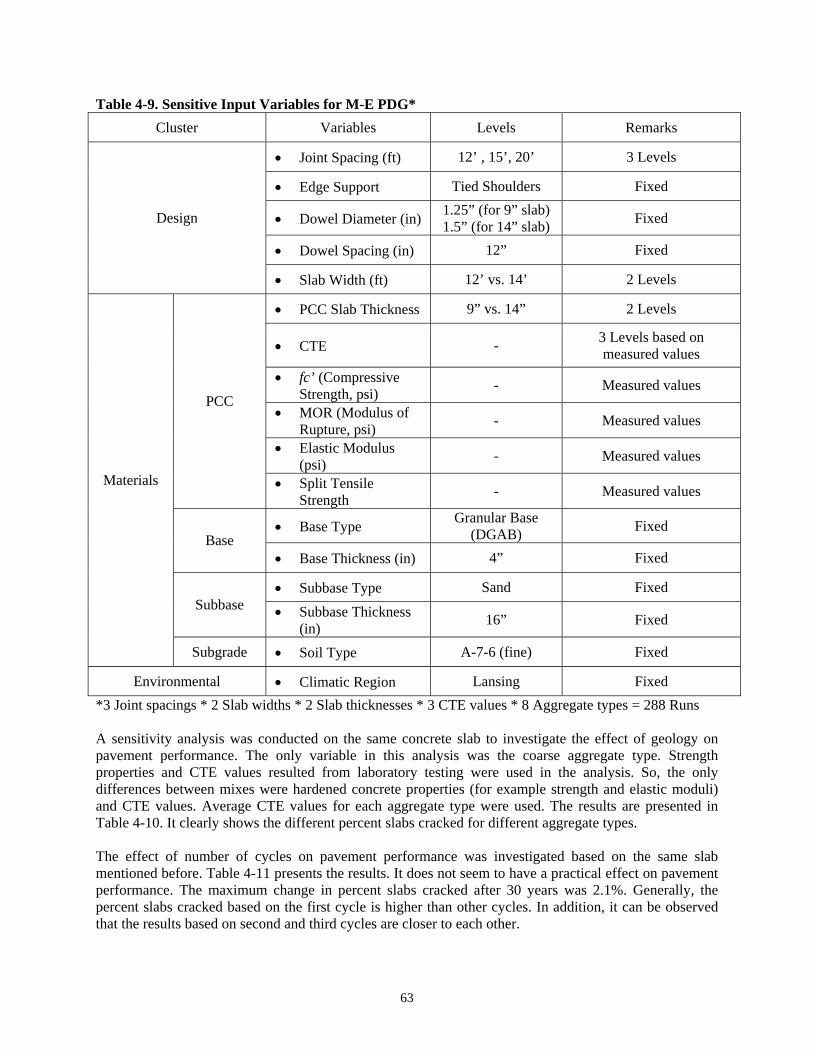
Table 4-9. Sensitive Input Variables for M-E PDG* ster ari v marks Clu V ables Le els Re

• t Spac g (ft) 1 , 15’ 3 Levels 2’ , 20’ Join in

• e Su h s Fixed Tied S oulderEdg pport

• el D ter 1.25” (for b) 1 r 1 b ixe9” sla F d Dow iame (in) .5” (fo 4” sla )

• el ( 12” Fixed Dow Spacing in)

Design

• Wi vs evSlab dth (ft) 12’ . 14’ 2 L els

• Sla kn s 2 Levels 9” v . 14” PCC b Thic ess

• measured values 3 Levels based on - CTE

• Com ivengt fc’ ( press - Measured valuesStre h, psi)

• re, - Measured values MOR (Modulus of

Ruptu psi)• l c M lus

(p - Measured values E asti odusi)

PCC

• p TenSt gt - Measured S lit sile valuesren h

• Base Typ l GA Fixed G nura ar seBae (D B) Base

• Base Thickness (i 4” Fixed n)

• Sand Fixed Subbase Type Subbase • Su s ne

(in 16” Fixed bba e Thick ss )

Materials

Subgrade • o ype -6 (f ) ixeil T A-7 ine F d S

Environme • C nsin Fixed ntal La g limatic Region *3 Joint spacings * 2 Slab width 2 ues Ag te ty 288

sensitivity analysis was conducted on the same concrete slab to investigate the effect of geology on avement performance. The only variable in this analysis was the coarse aggregate type. Strength roperties and CTE values resulted from laboratory testing were used in the analysis. So, the only ifferences between mixes were hardened concrete properties (for example strength and elastic moduli) nd CTE values. Average CTE values for each aggregate type were used. The results are presented in able 4-10. It clearly shows the different percent slabs cracked for different aggregate types.

he effect of number of cycles on pavement performance was investigated based on the same slab entioned before. Table 4-11 presents the results. It does not seem to have a practical effect on pavement

erformance. The maximum change in percent slabs cracked after 30 years was 2.1%. Generally, the ercent slabs cracked based on the first cycle is higher than other cycles. In addition, it can be observed at the results based on second and third cycles are closer to each other.

s * Slab thicknesses * 3 CTE val * 8 grega pes = Runs

AppdaT Tmppth

63

Table 4-10. Percent Slabs Cracked Based on CTE Values for Different Aggregate Types ent Age, Years PavemMix ID Aggregat TE 10 20 30 e Type CTE, µε/ºF C , µε/ºC 5

CTE 1 Limes 0 0 0 tone 4.75 8.55 0 CTE 2 Grav 1 0.7 4.3 13.2 el 5.93 0.67 0.1 CTE 3 itic L 0 0.1 0.3 Dolom imestone 4.56 8.21 0 CTE 4 Sla 1 0 0 0 g 5.81 0.46 0 CTE 5 Dolom 1 1.3 4 7.8 ite 6.01 0.82 0.4 CTE 6 Gabbro (Tr 0.2 1.1 3.7 ap Rock) 5.48 9.86 0 CTE 7 Dolom 1 0 0 0 ite 6.00 0.80 0 CTE 8 Dolom 1 0.5 2.8 8.3 ite 5.96 0.73 0.1

Table 4-11. Percent Slabs sed o lues for D nt C

Age, YeCracked Ba n CTE Va iffere ycles

Pavement ars Mix CyID Num

clb

CTEµε/ºF

, 20 omments e , CTE Cer µε/ºC 5 10 30

1 4.84 8.71 0 0 0 0 2 4.78 8.60 0 0 0 0 CTE 1 3 4.74 8 0

Number of cycles does not have an effect on this mix.

.53 0 0 0 1 5.97 0.1 0.8 4.8 14.4 10.75 2 5.8 10 4.1 12.6 91 .60 0.1 0.7 CTE 2

5. 1 4.0 12.ack

ter s f mi3 90 0.62 0.1 0.6 3 af

There is a difference in % slabs cr

maximum of 2.1% ed

30 year or this x. 1 4. 0.1 0.4 61 8.30 0 0 2 4. 0.1 0.3 54 8.17 0 0 CTE 3 3 4. 0.1 0.3

Number of cycles has a very all effect on this mix

.1%sm(0 ). 51 8.12 0 0

1 5.88 1 0 0.58 0 0 0 2 5. 1 080 0.44 0 0 0 C3 5. 1 0

mbve a ct o mix

Nuha

er of cycles does not n effe n this . TE 4

80 0.44 0 0 0 1 1 8.9 6.07 0.93 0.5 1.5 4.6 2 5.99 1 7.30.78 0.4 1.2 3.7 CTE 5 3 1 7

There is a maximum of 1.9% ffer % rac

after 30 years for this mix. 5.97 0.75 0.4 1.2 di ence in slabs c ked

3.6 1 5.50 9.90 0 0.2 1.2 3.9 2 5.48 9.86 0 0.2 1.1 3.7 CTE 6 3 5.48 0 0.2 1 3

Number of cycles has a very small (0.2%) effect on %

ab d.1 .7 sl s cracke . 9.86 1 6.09 10 0 0 0 .96 0 2 5.96 10 0 0 0 .73 0 CTE 7 3 5.94 10 0

Num cy s have an effect on th

.69 0 0 0

ber of cles doeis m

not ix.

1 5.96 10 .73 0.1 0.5 2.8 8.3 2 5.94 10.69 0.1 0.4 2.6 7.9 CTE 8 3 5.92 10 2 7.5

There is a maximum of 0.8% difference in % slabs craafter 30 years for this mix. 0.1 0.4 .5

cked .66

For the analysis regarding impact of CTE of concre with different ages on pavement performance, the same pavement mentioned before was considered. For each of the aggregate types, average CTE values at 14, 28, and 90 days were selected. The results of th G analysis are shown in Table 4-12. The difference in percent slabs cracked ranged from 0 to 6.1% after 30 years. The overall effect of CTE on percent slabs cracked based on the results does not seem to be significant (operational) for this typical design. Based on this limited analysis, the author recommends the measurement of CTE at 28 days to be considered in pavement design.

te

e M-E PD

64

Table 4-12. Percent Slabs Cracked Based on CTE Values for Different Ages , YePavement Age ars M

Age, Day µε/ºF 20 mments ix

ID s CTE,

µε/ºC CTE,

5 10 30 Co

14 4.52 0 8.13 0 0 0 28 4.54 0 8.18 0 0 0 CTE 1 90 4.77 0

g ime of testing does not have an effect on this mix. 8.59 0 0 0

A e at the t

14 5.87 3.7 10.57 0.1 0.6 11.5 28 5.84 3.4 10.52 0.1 0.5 10.7 CTE 2 90 5.96 4.7

h um of 3.5% difference in % slabs cracked aft rs for this mix. 10.73 0.1 0.8 14.2

T ere is a maxim

er 30 yea14 4.50 0.1 8.10 0 0 0.3 28 4.51 0.1 8.11 0 0 0.3 CTE 3 90 4.56 1 0.1 .3

Age at the time of testing does not have an effect on this mix. 8.2 0 0 0

14 5.56 0 10.01 0 0 0 28 5.71 0 10.27 0 0 0 CTE 4 90 6.01 1 0 0

Age at the time of testing does not have an effect on this mix. 10.8 0 0

14 5.86 10.55 0.3 0.9 2.7 5.2 28 5.92 10.65 0.3 1 3.2 6.2 CTE 5 90 6.11 1 9.8

There is a maximum of 4.6% difference in % slabs cracked

0.99 0.5 1.7 5 after 30 years for this mix. 14 1 .85.49 9.89 0 0.2 .1 3 28 5.41 9 0 0.9 3 .73 0 .1 CTE 6

5.47 1 .6

e ga very small (0.8%) effect on

lab ked.90 9.85 0 0.2 .1 3 % s

Age at the tim of testin has

s crac 14 5.92 10 .65 0 0 0 0 28 5.90 10 0 0 .62 0 0 CTE 7 90 5.96 1 0

Age at the time of testing does ha ffect on this 0.73 0 0 0 not ve an e mix.

14 5.66 1 1 .5 0.19 0 0.2 . 31 28 5.87 1 2 .40.57 0.1 0.3 .1 6 CTE 8 90 1 3 .6

There is a maximum of 6.1% fere % s rack

after 30 years for this mix. 6.02 0.84 0.1 0.5 .2 9dif nce in labs c ed

s s 4 as pe vest the s of

and other design fe lo performa th rete pavement. The details about the ariables and levels used in the sensitivity analysis are summarized in Table 4-9. CTE values for each

type of aggregate were the maximum, the minimum, and the average measured values. Actual mix design proportions were used as inputs. Elastic modulus and modulus of rupture values were obtained from laboratory tests. Initial two-way average annual daily truck traffic (AADTT) was considered to be 6000. In order to investigate the effect of the variables presented in Table 4-9 on performance of concrete pavement (cracking), an analysis of variance (ANOVA) was performed on each set of designs with same aggregate type. Based on the outcome of these analyses, the statistical significance of different variables and their interactions were obtained. A variable or an interaction is statistically significant if the p-value is less than 0.05 (a confidence level of 95%). The practical significance (is defined in the subsequent paragraphs) of the significant variables was then studied. Here, only the variables with both statistical and practical significance were selected for the investigation. The results (ANOVA, main effect, and interaction effect tables) are shown in Tables 4-14 to 4-21. Variables and interactions that are both statistically and practically significant are highlighted in the ANOVA tables and are presented in the interaction effect tables. ∆MAX in the main and interaction effect tables (tables b and c for each aggregate type) is the maximum difference in percent slabs cracked for the given levels of the variables. The main effects show the impact of a particular variable on percent slabs cracked for a given number of years (age of the pavement). The interaction effects show the effect of a combination of two or three

For the last analysi , a factorial (a shown in Table -9) w develo d to in igate effect CTE atures on the ng term nce of e conc

v

65

variables on pavement cracking. The Federal Highway Administration (FHWA) has specified percent slabs cracked at t , 10 of av a w levels of criteria (good to n ormal to poor) (2 rit e s in d in percent slabs cracked between two criteria levels. T same proac was used to produce following tables in order to investigate the effects on cracking performance. he pr s investigated by comparing the percent slabs cracked wi specif FH alues. It can be seen from these tables that, thinner slab, lo r jo ci d CT ues increased percent of abs cracke er the of m c o be seen from a numanalyses that when comparing the effect of CTE c e th ct of slab thickness or joint spacing, the combined effect of C nd jo cin or fic an fect E a b thickness based on the investigated levels. Table 4-13. FHWA Cracking Criteria for Rigid Pa nt

em ge ( )

he end of 5 , 20, and 30 1). These c

yearseria ar

rigid phown

ement Table 4-13. In this table,

ge for t o ormal and n ∆ is the ifference

he ap h T actical significance wa

th ied WA v

nge int spa ng, an higher E val lead tober of sl d ov age a pave ent. It

d an als

ombin with e effeTE a int spa g is m e signi ant th the ef of CT nd sla

veme s (21) Pav ent A yearsPerformance Criteria 10 20 30 Measure 0 5

Good-Normal 0 5 1.2 2.5 5 7.5 Norm or 5 10 15 al-Po 0 2.5

∆ 0 1.25 2.5 5 7.5 Increase/year 0.5 0.5 0.5 0.5

Cracking (% S

rage se/ 0.5

labs Cracked)

Ave Increa year Abbreviations used in the following tables a

la ick t sp , SW = Slab w T oe t o al sio

re:

ST = S b th ness, JS = Join acing idth, C E = C fficien f therm expan n

66

Table 4-14 a. CTE 1 ANOVA Results DF Anov F ValueSource a SS Mean Square P Value

S 25 62 0.02T 1 4.62 4. 25 8.03 98 JS 2 9.245 2 8.03 0.0201 4.62 5SW 1 1.5625 6 0.1.5 25 2.71 1506 CTE 5 3 3.7 0.0896 2 4.26 2.1 25ST*JS 2 9.245 0.4.6225 8.03 0201 ST*SW 1 1.5625 6 0.1.5 25 2.71 1506 ST*CTE 5 3 3.7 0.0896 2 4.26 2.1 25JS*SW 2 3.125 6 2 0.11.5 25 .71 448 JS*CTE 4 3 3 3.7 0.0751 8.5 2.1 25SW*CTE 1 7 3 1 0.4219 2 1. 516666 0.57583 33ST*JS*SW 2 3.125 6 2 0.11.5 25 .71 448 ST*JS*CTE 3 3 3.7 0.0751 4 8.5 2.1 25JS*SW*CTE 4 2.30333333 0.57583333 1 0.4752 Table 4-14 b. CTE 1 Main Effects

Mean Percent Slabs Cracked Maximum Mean Differences Variable▼ Level

5 yr 10 yr 20 yr 30 yr ∆MAX 5 ∆MAX 10 ∆MAX 20 ∆MAX 30

14 0 0 0 0 Slab Thickness (in) 9 0.02 0.07 0.29 0.72

0.02 0.07 0.29 0.72

12 0 0 0 0 15 0 0 0 0 Joint Spacing (ft) 20 0.03 0.11 0.43 1.08

0.03 0.11 0.43 1.08

14 0.01 0.01 0.06 0.15 Slab Width (ft) 12 0.02 0.06 0.23 0.57

0.01 0.05 0.18 0.42

4.42 (7.96) 0 0.01 0.03 0.07 4.69 (8.44) 0.01 0.02 0.07 0.17 CTE, µε/˚F (µε/˚C) 5.12 (9.22) 0.03 0.08 0.34 0.84

0.03 0.08 0.32 0.78

67

Table 4-15 a. CTE 2 ANOVA Results Source DF Ano n S ava SS Mea quare F V lue P Value

ST 1 1044 4 6 21.43361 10 41.433 1 61 .65 <.0001 JS 2 26380.0 6 0 8 773.9405 1319 .0202 2 <.0001 SW 1 294. 5 29 5 17.2 0 122 4.122 6 .006CTE 2 1833.6 6 91 2 5 0.0001 705 6.835 8 3.8ST*JS 2 7658.5 9 8 94 24338 3 29.266 2 .68 <.0001 ST*SW 1 55.0 4 5 9 3 0069 5.006 4 .23 .1225 ST*CTE 2 6.2 6 2 0 0.8376 205 3.110 8 .18JS*SW 2 17 5 75 5 0.0513 3.01 86.50 .08JS*CTE 4 2 4 21 11 12841. 444 0.311 .34 0.0047 SW*CTE 2 5 5 7 1 0.2515 9.73 29.86 5 .75ST*JS*SW 2 393.6 2 19 61 11 0.0088 372 6.818 .55ST*JS*CT 62.8 4 64 11 37E 4 25 244 0.706 .59 0.0002 JS*SW*CTE 4 2 4 0 0.7775 29.9 7. 8 .44

Table 4-15 b. CTE 2 Main Effects M Perc ab k xi ea ereean ent Sl s Crac ed Ma mum M n Diff nces

Variable▼ Lev5 10 20 30 ∆ MAX 10 MAX 20 MAX 30

el ∆ ∆ ∆yr yr yr yr MAX 5

14 0.19 0.93 4.37 9.23 Slab Thickness (in) 9 22 30. 37 43

2 2 6 77 .39 .29

2.37 29.83 33.0 34.0.56

1 0.0 0. 02 0 3 14 .47 15 0.28 1.37 6.76 14.67 Jo p g2 33 46. 55 63

3 55.6 63.19 int S acin (ft) 33.86 46.10 .86 16 .74 .66

14 9. 14 19 293 .7 .04 3.41 Slab Width (ft) 12 12 1 22 29

2.9 2.3 3.68 5.72.83 7 .72 .12

5.29 (9.52) 5. 12 6 174 .56 1 .51 8.18 5.91 (1 ) 12 16 9 20.64 .65 .41 1 .76 5.07 CTE, µε/˚F (µε/˚C) 6.42 (11.56) 15.74 8.5 26.3 35.

6 8 54

10 6.03 9.87 17.3 1 8

68

Table 4-15 c. CTE 2 Interaction Effects

Variables ST, CTE Level

JS, ST Level 5 yr 10 yr 20 yr 30 yr ∆MAX 5 ∆MAX 10 ∆MAX 20 ∆MAX 30

12 0 0 0 0 15 0 0 0 0 14 20 0.58 2.8 13.12 27.7

0.583 2.8 13.12 27.7

12 0 0.05 0.283 0.93 15 0.55 2.73 13.52 29.3

ST JS

9 20 67.13 89.52 98.37 99.6

67.13 89.47 98.08 98.68

12 0.00 0.00 0.03 0.08 15 0.05 0.20 1.13 3.53 5.29 (9.52) 20 17.18 37.48 48.38 50.95

17.18 37.48 48.35 50.88

12 0.00 0.03 0.10 0.33 15 0.18 0.93 5.23 13.485.91 (10.64) 20 37.78 48.28 53.95 61.40

37.78 48.25 53.85 61.08

12 0.00 0.05 0.30 1.00 15 0.60 2.98 13.93 27.00

CTE JS

6.42 (11.56) 20 46.63 52.73 64.90 78.63

46.63 52.68 64.60 77.63

12 0 0 0 0 15 0 0 0 0 14 20 0 0.15 0.95 2.95

0 0.15 0.45 0.95

12 0 0 0.05 0.15 15 0.1 0.4 2.25 7.05

5.29 (9.52)

9 20 34.35 74.8 95.8 98.95

34.4 74.8 90.2 95.75

12 0 0 0 0 15 0 0 0 0 14 20 0.3 1.5 8.5 22.9

0.3 1.5 4.1 8.5

12 0 0.05 0.2 0.65 15 0.35 1.85 10.45 26.95

5.91 (10.64)

9 20 75.25 95.05 99.4 99.9

75.3 95 98.4 99.2

12 0 0 0 0 15 0 0 0 0 14 20 1.45 6.75 29.9 57.25

1.45 6.75 16.6 29.9

12 0 0.1 0.6 2 15 1.2 5.95 27.85 54

CTE ST JS

6.42 (11.56)

9 20 91.8 98.7 99.9 100

91.8 98.6 99.3 99.3

69

Table 4-16 a. CTE 3 ANOVA Results Source DF Anova SS Mean Square F Value P Value

ST 1 7321.65444 7321.65444 199.9 <.0001 JS 2 12859.29389 6429.64694 175.54 <.0001 SW 1 202.58778 202.58778 5.53 0.0569 CTE 2 360.98722 180.49361 4.93 0.0542 ST*JS 2 12519.77389 6259.88694 170.91 <.0001 ST*SW 1 191.36111 191.36111 5.22 0.0623 ST*CTE 2 324.72056 162.36028 4.43 0.0658 JS*SW 2 173.11056 86.55528 2.36 0.175 JS*CTE 4 547.80444 136.95111 3.74 0.0737 SW*CTE 2 47.68722 23.84361 0.65 0.5548 ST*JS*SW 2 159.25722 79.62861 2.17 0.1949 ST*JS*CTE 4 489.35111 122.33778 3.34 0.0914 JS*SW*CTE 4 153.91444 38.47861 1.05 0.4548

Table 4-16 b. CTE 3 Main Effects

Mean Percent Slabs Cracked Maximum Mean Differences Variable▼ Level

5 yr 10 yr 20 yr 30 yr ∆MAX 5 ∆MAX 10 ∆MAX 20 ∆MAX 30

14 0 0.01 0.06 0.18 Slab Thickness (in) 9 3.02 10.31 21.91 28.7

3.02 10.31 21.86 28.52

12 0 0 0.03 0.08 15 0.03 0.14 0.73 2.1 Joint Spacing (ft) 20 4.5 15.33 32.2 41.14

4.5 15.33 32.18 41.07

14 0.74 3.38 8.68 12.07 Slab Width (ft) 12 2.28 6.93 13.29 16.81

1.54 3.55 4.61 4.74

4.10 (7.38) 0.28 1.19 5.37 10.13 4.53 (8.15) 1.01 4.43 11.91 15.53 CTE, µε/˚F (µε/˚C) 4.92 (8.86) 3.25 9.85 15.68 17.66

2.98 8.66 10.31 7.53

Table 4-16 c. CTE 3 Interaction Effects Variables ST Level JS Level 5 yr 10 yr 20 yr 30 yr ∆MAX 5 ∆MAX 10 ∆MAX 20 ∆MAX 30

12 0 0 0 0 15 0 0 0 0 14 20 0 0.0167 0.167 0.53

0 0.017 0.167 0.533

12 0 0 0.05 0.15 15 0.0667 0.2833 1.45 4.2

ST JS

9 20 9 30.65 64.23 81.8

9 30.65 64.18 81.6

70

Table 4-17 a. CTE 4 ANOVA Results Source DF Anova SS Mean Square F Value P Value

ST 1 2062.673611 2062.673611 1585.99 <.0001 JS 2 4113.251667 2056.625833 1581.34 <.0001 SW 1 134.946944 134.946944 103.76 <.0001 CTE 2 361.931667 180.965833 139.15 <.0001 ST*JS 2 4107.207222 2053.603611 1579.02 <.0001 ST*SW 1 134.173611 134.173611 103.17 <.0001 ST*CTE 2 360.383889 180.191944 138.55 <.0001 JS*SW 2 265.273889 132.636944 101.98 <.0001 JS*CTE 4 721.541667 180.385417 138.7 <.0001 SW*CTE 2 2.603889 1.301944 1 0.4215 ST*JS*SW 2 263.740556 131.870278 101.4 <.0001 ST*JS*CTE 4 718.452778 179.613194 138.1 <.0001 JS*SW*CTE 4 5.202778 1.300694 1 0.4752

Table 4-17 b. CTE 4 Main Effects

Mean Percent Slabs Cracked Maximum Mean Differences Variable▼ Level

5 yr 10 yr 20 yr 30 yr ∆MAX 5 ∆MAX 10 ∆MAX 20 ∆MAX 30

14 0 0 0 0.01 Slab Thickness (in) 9 0.87 3.12 9.22 15.14

0.87 3.12 9.22 15.14

12 0 0 0 0 15 0 0 0.01 0.03 Joint Spacing (ft) 20 1.31 4.68 13.83 22.69

1.31 4.68 13.83 22.69

14 0.22 0.89 3.07 5.64 Slab Width (ft) 12 0.65 2.23 6.15 9.51

0.43 1.34 3.08 3.87

5.42 (9.76) 0.12 0.45 1.73 3.68 5.75 (10.35) 0.34 1.28 4.27 7.59 CTE, µε/˚F (µε/˚C) 6.07 (10.93) 0.85 2.95 7.84 11.45

0.73 2.5 6.12 7.77

71

Table 4-17 c. CTE 4 Interaction Effects

Variables ST, CTE Level

JS, SW, ST Level 5 yr 10 yr 20 yr 30 yr ∆MAX 5 ∆MAX 10 ∆MAX 20 ∆MAX 30

12 0 0 0 0 15 0 0 0 0 14 20 0 0 0 0.02

0 0 0 0.017

12 0 0 0 0 15 0 0 0.02 0.07

ST JS

9 20 2.62 9.35 27.65 45.4

2.62 9.35 27.65 45.37

12 0.00 0.00 0.00 0.01 14 14 0.00 0.00 0.00 0.00 0.00 0.00 0.00 0.01

12 1.30 4.46 12.30 19.01 ST SW 9 14 0.44 1.78 6.14 11.28 0.86 2.68 6.16 7.73

14 0 0 0 0 5.42 (9.76) 9 0.23 0.9 3.45 7.37 0.23 0.9 3.45 7.37

14 0 0 0 0 5.75 (10.35) 9 0.68 2.55 8.53 15.2 0.68 2.55 8.53 15.18

14 0 0 0 0.02

CTE ST

6.07 (10.93) 9 1.7 5.9 15.68 22.9 1.7 5.9 15.68 22.87

12 0.00 0.00 0.00 0.00 15 0.00 0.00 0.00 0.03 5.42 (9.76) 20 0.35 1.35 5.18 11.03

0.35 1.35 5.18 11.03

12 0.00 0.00 0.00 0.00 15 0.00 0.00 0.00 0.03 5.75 (10.35) 20 1.03 3.83 12.80 22.75

1.03 3.83 12.80 22.75

12 0.00 0.00 0.00 0.00 15 0.00 0.00 0.03 0.05

CTE JS

6.07 (10.93) 20 2.55 8.85 23.50 34.30

2.55 8.85 23.50 34.30

Table 4-18 a. CTE 5 ANOVA Results

Source DF Anova SS Mean Square F Value P Value ST 1 9847.25444 9847.25444 985.05 <.0001 JS 2 24329.07056 12164.53528 1216.86 <.0001 SW 1 202.58778 202.58778 20.27 0.0041 CTE 2 476.70889 238.35444 23.84 0.0014 ST*JS 2 10674.45056 5337.22528 533.9 <.0001 ST*SW 1 24.66778 24.66778 2.47 0.1673 ST*CTE 2 4.62889 2.31444 0.23 0.8001 JS*SW 2 115.03389 57.51694 5.75 0.0403 JS*CTE 4 237.76111 59.44028 5.95 0.0278 SW*CTE 2 35.24222 17.62111 1.76 0.2499 ST*JS*SW 2 275.34722 137.67361 13.77 0.0057 ST*JS*CTE 4 667.98111 166.99528 16.71 0.0021 JS*SW*CTE 4 18.39111 4.59778 0.46 0.7639

72

Table 4-18 b. CTE 5 Main Effects Mean Percent Slabs Cracked Maximum Mean Differences

Variable▼ Level 5 yr 10 yr 20 yr 30 yr ∆MAX 5 ∆MAX 10 ∆MAX 20 ∆MAX 30

14 0.43 1.29 3.59 6.3 Slab Thickness (in) 9 29.28 33.18 36.46 39.38

28.85 31.89 32.87 33.08

12 0.01 0.03 0.1 0.18 15 0.58 1.78 5.12 9.09 Joint Spacing (ft) 20 43.98 49.89 54.86 59.24

43.98 49.86 54.76 59.06

14 13.77 16.34 18.47 20.47 Slab Width (ft) 12 15.95 18.13 21.58 25.21

2.18 1.79 3.11 4.74

5.63 (10.13) 12.83 15.76 17.46 18.77 5.96 (10.73) 15.13 17.14 19.53 22.15 CTE, µε/˚F (µε/˚C) 6.30 (11.34) 16.61 18.81 23.09 27.6

3.78 3.05 5.63 8.83

73

Table 4-18 c. CTE 5 Interaction Effects

Variables ST, CTE, JS Level

JS, SW, JS Level 5 yr 10 yr 20 yr 30 yr ∆MAX 5 ∆MAX 10 ∆MAX 20 ∆MAX 30

12 0 0 0 0 15 0 0 0 0 14 20 1.3 3.87 10.77 18.9

1.3 3.867 10.77 18.9

12 0.017 0.067 0.2 0.37 15 1.17 3.57 10.23 18.2

ST JS

9 20 86.67 95.92 98.95 99.6

86.65 95.85 98.75 99.22

12 0.00 0.03 0.03 0.08 15 0.20 0.65 1.98 3.85 5.63 (10.13) 20 38.30 46.60 50.38 52.38

38.30 46.58 50.35 52.30

12 0.00 0.03 0.10 0.15 15 0.50 1.48 4.43 8.23 5.96 (10.73) 20 44.90 49.93 54.05 58.08

44.90 49.90 53.95 57.93

12 0.03 0.05 0.18 0.33 15 1.05 3.23 8.95 15.20

CTE JS

6.30 (11.34) 20 48.75 53.15 60.15 67.28

48.73 53.10 59.98 66.95

12 0.00 0.00 0.00 0.00 12 14 0.00 0.00 0.00 0.00 0.00 0.00 0.00 0.00

12 0.00 0.00 0.00 0.00 15 14 0.00 0.00 0.00 0.00 0.00 0.00 0.00 0.00

12 1.70 5.03 13.77 23.53

14

20 14 0.90 2.70 7.77 14.27 0.80 2.33 6.00 9.27

12 0.03 0.13 0.33 0.63 12 14 0.00 0.00 0.07 0.10 0.03 0.13 0.27 0.53

12 1.87 5.60 15.73 27.2015 14 0.47 1.53 4.73 9.17 1.40 4.07 11.00 18.03

12 92.10 98.03 99.63 99.90

ST JS SW

9

20 14 81.23 93.80 98.27 99.27 10.87 4.23 1.37 0.63

12 0 0 0 0 15 0 0 0 0 14 20 0.3 1 2.85 5.6

0.3 1 2.85 5.6

12 0 0.05 0.05 0.15 15 0.4 1.3 3.95 7.7

5.63 (10.13)

9 20 76.3 92.2 97.9 99.15

76.3 92.15 97.85 99

12 0 0 0 0 15 0 0 0 0 14 20 1 3 8.85 16.45

1 3 8.85 16.45

12 0 0.05 0.2 0.3 15 1 2.95 8.85 16.45

5.96 (10.73)

9 20 88.8 96.85 99.25 99.7

88.8 96.8 99.05 99.4

12 0 0 0 0 15 0 0 0 0 14 20 2.6 7.6 20.6 34.65

2.6 7.6 20.6 34.65

12 0.05 0.1 0.35 0.65 15 2.1 6.45 17.9 30.4

CTE ST JS

6.30 (11.34)

9 20 94.9 98.7 99.7 99.9

94.85 98.6 99.35 99.25

74

Table 4-19 a. CTE 6 ANOVA Results Source DF Anova SS Mean Square F Value P Value

ST 1 10441.43361 10441.43361 612.65 <.0001 JS 2 26380.04056 13190.02028 773.92 <.0001 SW 1 294.1225 294.1225 17.26 0.006 CTE 2 1833.67056 916.83528 53.8 0.0001 ST*JS 2 7658.53389 3829.26694 224.68 <.0001 ST*SW 1 55.00694 55.00694 3.23 0.1225 ST*CTE 2 6.22056 3.11028 0.18 0.8376 JS*SW 2 173.015 86.5075 5.08 0.0513 JS*CTE 4 841.24444 210.31111 12.34 0.0047 SW*CTE 2 59.735 29.8675 1.75 0.2515 ST*JS*SW 2 393.63722 196.81861 11.55 0.0088 ST*JS*CTE 4 2562.82444 640.70611 37.59 0.0002 JS*SW*CTE 4 29.92 7.48 0.44 0.7775 Table 4-19 b. CTE 6 Main Effects

Mean Percent Slabs Cracked Maximum Mean Differences Variable▼ Level

5 yr 10 yr 20 yr 30 yr ∆MAX 5 ∆MAX 10 ∆MAX 20 ∆MAX 30

14 0.02 0.09 0.53 1.67 Slab Thickness (in) 9 15.12 27.36 33.35 36.22

15.11 27.27 32.82 34.54

12 0 0 0.03 0.09 15 0.04 0.23 1.46 4.58 Joint Spacing (ft) 20 22.67 40.93 49.34 52.16

22.67 40.93 49.32 52.07

14 5.71 12.49 16.27 17.68 Slab Width (ft) 12 9.43 14.96 17.62 20.21

3.72 2.47 1.35 2.53

5.19 (9.34) 5.02 11.91 16.18 17.63 5.46 (9.83) 8.24 14.32 17.13 19.18 CTE, µε/˚F (µε/˚C) 5.56 (10.01) 9.45 14.94 17.52 20.03

4.43 3.03 1.33 2.4

Table 4-19 c. CTE 6 Interaction Effects Variables ST, CTE Level JS Level 5 yr 10 yr 20 yr 30 yr ∆MAX 5 ∆MAX 10 ∆MAX 20 ∆MAX 30

12 0 0 0 0 15 0 0 0 0 14 20 0.05 0.2667 1.6 5.02

0.05 0.267 1.6 5.017

12 0 0 0.05 0.18 15 0.0833 0.4667 2.917 9.17

ST JS

9 20 45.283 81.6 97.08 99.3

45.28 81.6 97.03 99.12

75

Table 4-20 a. CTE 7 ANOVA Results Source DF Anova SS Mean Square F Value P Value

ST 1 3379.484444 3379.484444 4419.23 <.0001 JS 2 6751.226667 3375.613333 4414.17 <.0001 SW 1 148.84 148.84 194.63 <.0001 CTE 2 159.171667 79.585833 104.07 <.0001 ST*JS 2 6735.742222 3367.871111 4404.05 <.0001 ST*SW 1 148.84 148.84 194.63 <.0001 ST*CTE 2 158.110556 79.055278 103.38 <.0001 JS*SW 2 292.826667 146.413333 191.46 <.0001 JS*CTE 4 316.856667 79.214167 103.59 <.0001 SW*CTE 2 1.635 0.8175 1.07 0.4008 ST*JS*SW 2 292.826667 146.413333 191.46 <.0001 ST*JS*CTE 4 314.737778 78.684444 102.89 <.0001 JS*SW*CTE 4 3.453333 0.863333 1.13 0.425 Table 4-20 b. CTE 7 Main Effects

Mean Percent Slabs Cracked Maximum Mean Differences Variable▼ Level

5 yr 10 yr 20 yr 30 yr ∆MAX 5 ∆MAX 10 ∆MAX 20 ∆MAX 30

14 0 0 0 0.01 Slab Thickness (in) 9 1.19 4.36 12.49 19.39

1.19 4.36 12.49 19.38

12 0 0 0 0 15 0 0 0.02 0.03 Joint Spacing (ft) 20 1.78 6.54 18.72 29.07

1.78 6.54 18.72 29.07

14 0.32 1.28 4.37 7.67 Slab Width (ft) 12 0.87 3.08 8.12 11.73

0.56 1.79 3.76 4.07

5.72 (10.30) 0.28 1.09 3.84 7.04 5.94 (10.69) 0.54 2.04 6.2 9.88 CTE, µε/˚F (µε/˚C) 6.15 (11.07) 0.97 3.41 8.69 12.18

0.69 2.32 4.85 5.14

Table 4-20 c. CTE 7 Interaction Effects Variables ST, CTE Level JS, ST Level 5 yr 10 yr 20 yr 30 yr ∆MAX 5 ∆MAX 10 ∆MAX 20 ∆MAX 30

12 0 0 0 0 15 0 0 0 0 14 20 0 0 0 0.03

0 0 0 0.033

12 0 0 0 0 15 0 0 0.033 0.07

ST JS

9 20 3.5667 13.083 37.43 58.1

3.567 13.08 37.43 58.1

14 0 0 0 0 5.72 (10.30) 9 0.55 2.1833 7.683 14.1 0.55 2.183 7.683 14.08

14 0 0 0 0.02 5.94 (10.69) 9 1.0833 4.0833 12.4 19.7 1.083 4.083 12.4 19.72

14 0 0 0 0.02

CTE ST

6.15 (11.07) 9 1.9333 6.8167 17.38 24.4 1.933 6.817 17.38 24.33

76

Table 4-21 a. CTE 8 ANOVA Results Source DF Anova SS Mean Square F Value Pr > F

ST 1 10380.21361 10380.21361 1018.33 <.0001 JS 2 22449.10722 11224.55361 1101.17 <.0001 SW 1 191.8225 191.8225 18.82 0.0049 CTE 2 345.02389 172.51194 16.92 0.0034 ST*JS 2 12149.94056 6074.97028 595.97 <.0001 ST*SW 1 38.23361 38.23361 3.75 0.1009 ST*CTE 2 1.17056 0.58528 0.06 0.9447 JS*SW 2 116.81167 58.40583 5.73 0.0406 JS*CTE 4 166.54611 41.63653 4.08 0.0619 SW*CTE 2 30.61167 15.30583 1.5 0.296 ST*JS*SW 2 244.33389 122.16694 11.98 0.008 ST*JS*CTE 4 442.73278 110.68319 10.86 0.0065 JS*SW*CTE 4 18.56167 4.64042 0.46 0.7669

Table 4-21 b. CTE 8 Main Effects

Mean Percent Slabs Cracked Maximum Mean Differences Variable▼ Level

5 yr 10 yr 20 yr 30 yr ∆MAX 5 ∆MAX 10 ∆MAX 20 ∆MAX 30

14 0.07 0.32 1.77 4.72 Slab Thickness (in) 9 18.21 28.59 34.56 38.68

18.14 28.27 32.79 33.96

12 0 0.02 0.07 0.21 15 0.13 0.59 3.14 8.18 Joint Spacing (ft) 20 27.28 42.76 51.28 56.72

27.28 42.74 51.21 56.51

14 7.25 13.17 16.93 19.39 Slab Width (ft) 12 11.02 15.74 19.39 24.01

3.77 2.57 2.46 4.62

5.46 (9.83) 5.1 11.77 16.23 18.02 5.87 (10.57) 9.84 15.18 18.16 21.5 CTE, µε/˚F (µε/˚C) 6.13 (11.03) 12.47 16.43 20.1 25.59

7.37 4.66 3.88 7.58

77

Table 4-21 c. CTE 8 Interaction Effects

Variables ST, JS, CTE Level

JS, SW, ST Level 5 yr 10 yr 20 yr 30 yr ∆MAX 5 ∆MAX 10 ∆MAX 20 ∆MAX 30

12 0 0 0 0 15 0 0 0 0 14 20 0.2 0.97 5.3 14.2

0.2 0.967 5.3 14.17

12 0 0.03 0.13 0.42 15 0.25 1.18 6.28 16.4

ST JS

9 20 54.37 84.55 97.25 99.3

54.37 84.52 97.12 98.85

12 0.00 0.00 0.00 0.00 12 14 0.00 0.00 0.00 0.00 0.00 0.00 0.00 0.00

12 0.00 0.00 0.00 0.00 15 14 0.00 0.00 0.00 0.00 0.00 0.00 0.00 0.00

12 0.27 1.30 6.97 18.00

14

20 14 0.13 0.63 3.63 10.33 0.13 0.67 3.33 7.67

12 0.00 0.07 0.23 0.73 12 14 0.00 0.00 0.03 0.10 0.00 0.07 0.20 0.63

12 0.43 1.93 10.13 25.5015 14 0.07 0.43 2.43 7.23 0.37 1.50 7.70 18.27

12 65.43 91.13 99.00 99.83

ST JS SW

9

20 14 43.30 77.97 95.50 98.70 22.13 13.17 3.50 1.13

12 0.00 0.00 0.00 0.00 15 0.00 0.00 0.00 0.00 14 20 0.05 0.15 1.00 3.10

0.05 0.15 1.00 3.10

12 0.00 0.00 0.05 0.15 15 0.10 0.40 2.20 6.50

5.63 (10.13)

9 20 30.45 70.05 94.10 98.35

30.45 70.05 94.05 98.20

12 0.00 0.00 0.00 0.00 15 0.00 0.00 0.00 0.00 14 20 0.15 0.80 4.50 12.90

0.15 0.80 4.50 12.90

12 0.00 0.05 0.10 0.40 15 0.25 1.10 5.95 16.10

5.96 (10.73)

9 20 58.65 89.10 98.40 99.60

58.65 89.05 98.30 99.20

12 0.00 0.00 0.00 0.00 15 0.00 0.00 0.00 0.00 14 20 0.40 1.95 10.40 26.50

0.40 1.95 10.40 26.50

12 0.00 0.05 0.25 0.70 15 0.40 2.05 10.70 26.50

CTE ST JS

6.30 (11.34)

9 20 74.00 94.50 99.25 99.85

74.00 94.45 99.00 99.15

78

CHAPTER 5: CONCLUSIONS 5.1 Introduction In this chapter a summary of research conducted in this project is presented followed by findings and conclusions regarding CTE measurement and factors affecting it. Long term effects of CTE on the performance of jointed concrete pavements are also presented. Recommendations about CTE testing procedure are also presented in this chapter. 5.2 Summary of Work Performed This report documents the effect of eight different coarse aggregate sources on the CTE of a typical MDOT concrete paving mixture. Over 700 concrete specimens were fabricated for various tests. At least three replicate specimens were fabricated for each test for a given test date. The test variables included in the laboratory investigation included the aggregate geology, the age of the sample at the time of testing, and the number of heating-cooling cycles applied to the sample. The details about the experimental program and the test method are documented in chapter 3. The results from the laboratory investigation and the impact of the test variables on the magnitude of CTE are documented in chapter 4 of the report. The impact of CTE on the structural design and performance of jointed concrete pavements was also investigated as part of this research study and the results are presented in chapter 4. 5.3 Factors Affecting Measurement of CTE The following conclusions were based on the laboratory investigation and the statistical analyses of the dataset;

• The magnitude of the measured CTE varied with aggregate geology. The measured CTE magnitudes for the various aggregate geologies compared favorably with the published values.

• Statistical analysis showed:

1) Magnitude of the measured CTE is significantly (statistically) influenced by the age of the sample at the time of testing.

2) Magnitude of the measured CTE at the early ages (3, 7, 14, 28 days) were significantly (statistically) different than the magnitudes determined at the end of 90, 180, and 365 days.

3) Operationally, the impact of this difference on transverse cracking (as computed by the M-E PDG software for 14, 28, and 90 days) was not found to be significant.

• The number of heating-cooling cycles in CTE test affects the magnitude of CTE. The CTE value calculated based on the first cycle was higher than the values calculated based on second and third cycles. Statistically the CTE values based on second and third cycles were not different from each other.

• Coefficient of variance for the data set ranged from 2-6%. Approximately 94% of the data set has a δCTE between ± 0.17 µε/oF (0.3 µε/oC). It was observed that, generally, concrete with higher CTE values is more sensitive to variability compared to concrete with low CTE values.

79

5.4 Impact of CTE on Long Term Pavement Performance M-E PDG software along with statistical analyses were used to investigate the impact of CTE value and its interaction with other design factors on long term performance of jointed concrete pavements in cracking. It was found that the impact of CTE, slab thickness, and joint spacing on transverse cracking were statistically significant. Practical significance was evaluated by comparing the results of the analyses with published criteria on percent slabs cracked. The selected practical significance criteria states that if a rigid pavement shows 7.5% slabs cracked after 30 years, it’s a good-normal slab. If it shows 15% slabs cracked, it’s a normal-poor slab. It was observed that, thinner slab, longer joint spacing, and higher CTE values resulted in increased percent of slabs cracked over the age of a pavement. Based on the results from a number of analyses, it was observed that when comparing the effect of CTE combined with the effect of slab thickness or joint spacing, the combined effect of CTE and joint spacing is more significant than the effect of CTE and slab thickness. 5.5 Suggested Recommendations The following recommendations are suggested:

• The CTE value based on one cycle is probably not reliable. It is suggested that the test specimen should be subjected to three test cycles of heating and cooling. The test data from cycles two or three should be used for the computation of CTE.

• Based on the operational significance analysis it is suggested that CTE measured at the end of 28 days can used as an input for jointed concrete pavement design.

• Automation of the temperature and displacement readings with a rate of one reading per minute (as recommended by Texas DOT test method 428-A) makes the testing process and CTE determination more reliable.

5.6. Recommended CTE Values The following table lists the CTE values for each coarse aggregate tested, based on the recommendations above: Table 5-1. Recommended CTE Values for Concrete Made with Different Coarse Aggregate

28-Day CTE (µε/oF ) 28-Day CTE (µε/oC) Mix ID Primary Aggregate Class Pit

Number Cycle #2 Cycle #3 Cycle #2 Cycle #3 CTE 1 Limestone 71-47 4.54 4.55 8.17 8.18 CTE 2 Gravel 19-56 5.84 5.84 10.51 10.52 CTE 3 Dolomitic Limestone 75-05 4.51 4.47 8.12 8.04 CTE 4 Slag 82-19 5.69 5.73 10.24 10.31 CTE 5 Dolomite 49-65 5.91 5.91 10.65 10.64 CTE 6 Gabbro (Trap Rock) 95-10 5.40 5.38 9.72 9.68 CTE 7 Dolomite 58-11 5.93 5.77 10.67 10.38 CTE 8 Dolomite 91-06 5.90 5.87 10.63 10.57

80

CHAPTER 6: REFERENCES

1. Mallela, J., Abbas, A., Harman, T., Chetna, R., Liu, R., and Darter, M., Measurement and Significance of the Coefficient of Thermal Expansion of Concrete in Rigid Pavement Design. Transportation Research Record: Journal of the Transportation Research Board No. 1919, Washington D.C., 2005.

2. Alungbe, G., Tia, M., and Bloomquist, D., Effects of Aggregate, Water/Cement Ratio, and Curing on the Coefficient of Linear Thermal Expansion of Concrete. Transportation Research Record: Journal of the Transportation Research Board No. 1335, Washington D.C., 1992.

3. Won, M., Improvements of Testing Procedures for Concrete Coefficient of Thermal Expansion. Transportation Research Record: Journal of the Transportation Research Board No. 1919, Washington D.C., 2005.

4. Naik, T. R., Chun Y., Kraus R. N., Investigation of Concrete Properties to Support Implementation of the New AASHTO Pavement Design Guide. Final Report. WHRP 06-14. Wisconsin Department of Transportation, 2006.

5. Hossain, M., Khanum, T., Tanesi, J., Scheiber, G., and Montney, R., The PCC Coefficient of Thermal Expansion Input for the Mechanistic-Empirical Pavement Design Guide. Proceedings of the 85th Transportation Research Board Annual Meeting, Washington D.C., 2006.

6. Tanesi, J., Kutay, M., Abbas, A., and Meininger, R., Effect of CTE Variability on Concrete Pavement Performance as Predicted using the Mechanistic-Empirical Pavement Design Guide. Proceedings of the 86th Transportation Research Board Annual Meeting, Washington D.C., 2007.

7. Kohler, E., Alvarado, R., and Jones, D., Measurement and Variability of Coefficient of Thermal Expansion for Concrete Pavements. Proceedings of the 86th Transportation Research Board Annual Meeting, Washington D.C., 2007.

8. Kohler, E., Kannekanti V., Influence of the Coefficient of Thermal Expansion on the Cracking of Jointed Concrete Pavements. University of California Pavement Research Center, Davis, California. Unpublished. 2007.

9. Loubser, P. J., Bryden J. G., An Apparatus for Determining the Coefficient of Thermal Expansion of Rocks, Mortars, and Concretes. Magazine of Concrete Research, Vol. 24, No. 79, June 1972.

10. U.S. Army Corps of Engineers, Test Method for Coefficient of Linear Thermal Expansion of Concrete. Cement and Concrete Handbook, CRD-C 39-81, June 1981.

11. Danish Technological Institute, Test Method Expansion Coefficient of Concrete. TI-B 101 (94), March 1994.

12. Childs, P., Wong, A. C. L., Gowripalan, N., Peng, G. D., Measurement of the Coefficient of Thermal Expansion of Ultra-High Strength Cementitious Composites using Fibre Optic Sensors. Cement and Concrete Research 37(2007) 789-795, February 2007

13. InstroTek.com

14. Sutter, L., Van Dam, T., Peterson, K., Mineral Characterization and Cataloging of Quarried Aggregate Sources Used in Michigan Highway Construction. Volume II: Materials Characterization Database, Michigan Department of Transportation, June 2003.

15. Polyscience.com

16. Iotech.com

81

17. Macrosensors.com

18. AASHTO, Standard Test Method for the Coefficient of Thermal Expansion of Hydraulic Cement Concrete. TP60-00, 2000.

19. ARA Inc., ERES Consultants Division, Guide for Mechanistic-Empirical Design of New and Rehabilitated Pavement Structures. Final Report, National Cooperative Highway Research Program, 1-37A, March 2004.

20. Kuehl, R.O., Design of Experiments: Statistical Principles of Research Design and Analysis. Duxbury Press, 2000.

21. Khazanovich, L., M. Darter, R. Bartlett, and T. McPeak, "Common Characteristics of Good and Poorly Performing PCC Pavements," Repot No. FHWA-RD-97-131, 1998.

82

APPENDIX A: SUMMARY OF DOT SURVEY Table A-1. Summary of DOT Survey

Questions Alabama DOT

Do you conduct CTE tests for your typical concrete paving mixtures? If yes, what test protocol does your agency follow?

No. ALDOT has initiated a research project with Auburn University to test the CTE of concrete mixtures typically used in the state. Tests are being performed in accordance with AASHTO TP 60.

How do you utilize your CTE information (for example, as an input into pavement design, aggregate acceptance, etc.)?"

This information is currently not being used.

What are the typical lithologies of the coarse aggregate used in concrete paving mixtures on state/federal funded projects? Example lithologies are (but not limited to): ultramafic, granite, schist, gneiss, limestone, dolomite, sandstone, slate, etc.

ALDOT mostly uses the following aggregates: siliceous river gravel, quartzite, high-calcium limestone, dolomitic limestone, granite, and sandstone.

What are the typical CTE ranges for concrete mixtures containing the various coarse aggregate lithologies stated in the previous question?

The only results available at this stage are for concrete made with river gravel: CTE = 12.5 x 10-6 in./in./°C.

In your experience with CTE testing, what other components of the concrete mix (fine aggregate, cement, cement replacements,etc) have a significant impact on the test results?

Coarse agg type and amount, fine agg type and amount, relative humidity, concrete age, and w/cm.

Do you have any research results, either published or unpublished, that you could send or provide the location on your website?

No. The research project with Auburn University is currently active and results will be made available when the research has been completed.

83

Table A-1. Summary of DOT Survey, continued Questions Alaska DOT Colorado DOT Kentucky DOT Maine DOT

Do you conduct CTE tests for your typical concrete paving mixtures? If yes, what test protocol does your agency follow?

No No No

Maine DOT does not currently utilize concrete pavement in our Highway Program.

How do you utilize your CTE information (for example, as an input into pavement design, aggregate acceptance, etc.)?"

N/A

What are the typical lithologies of the coarse aggregate used in concrete paving mixtures on state/federal funded projects? Example lithologies are (but not limited to): ultramafic, granite, schist, gneiss, limestone, dolomite, sandstone, slate, etc.

Sedimentary rocks including limestones, dolomites and

ravels.

g

What are the typical CTE ranges for concrete mixtures containing the various coarse aggregate lithologies stated in the previous question?

N/A

In your experience with CTE testing, what other components of the concrete mix (fine aggregate, cement, cement replacements,etc) have a significant impact on the test results?

N/A

Do you have any research results, either published or unpublished, that you could send or provide the location on your website?

No

84

Table A-1. Summary of DOT Survey, continued Questions Minnesota DOT NebraskaDOT New Hampshire DOT

Do you conduct CTE tests for your typical concrete paving mixtures? If yes, what test protocol does your agency follow?

No No We do not use concrete paving in NH

How do you utilize your CTE information (for example, as an input into pavement design, aggregate acceptance, etc.)?"

Aggregate type does not affect design N/A

What are the typical lithologies of the coarse aggregate used in concrete paving mixtures on state/federal funded projects? Example lithologies are (but not limited to): ultramafic, granite, schist, gneiss, limestone, dolomite, sandstone, slate, etc.

Typically: Limestone (including dolomites), gravels, granite, gneiss

Limestone

What are the typical CTE ranges for concrete mixtures containing the various coarse aggregate lithologies stated in the previous question?

Do not have values other than assumed values that are listed in literature

N/A

In your experience with CTE testing, what other components of the concrete mix (fine aggregate, cement, cement replacements,etc) have a significant impact on the test results?

No experience. Certainly ASR could result in expansion of beam specimens. The mix design including cement replacements would certainly affect results.

N/A

Do you have any research results, either published or unpublished, that you could send or provide the location on your website?

We are more concerned about thermal expansion in bridges than pavements. We have not experienced cracking problems that we can attribute to aggregate type.

N/A

85

Table A-1. Summary of DOT Survey, continued

Questions North Carolina DOT Oregon DOT Pennsylvania

DOT

South Dakota DOT

Do you conduct CTE tests for your typical concrete paving mixtures? If yes, what test protocol does your agency follow?

No No No No

How do you utilize your CTE information (for example, as an input into pavement design, aggregate acceptance, etc.)?"

No don’t use in current design process – spacing based on research

N/A

ME Pavement

Design Guide Input

What are the typical lithologies of the coarse aggregate used in concrete paving mixtures on state/federal funded projects? Example lithologies are (but not limited to): ultramafic, granite, schist, gneiss, limestone, dolomite, sandstone, slate, etc.

Predominantly granite and similar volcanics.

Limestone, dolomite, gravels

We have many types of coarse aggregates in the state. Their inclusion in concrete paving mix designs is based on quality test parameters. i.e. – sodium sulfate, amount of deleterious material, etc.

Limestone, Granite,

Quartzite.

What are the typical CTE ranges for concrete mixtures containing the various coarse aggregate lithologies stated in the previous question?

N/A N/A

3.8 x 10-6 / °F

(Limestone) 4.6 x 10-6 / °F (Granite)6.8 x 10-6 /

°F (Quartzite)

In your experience with CTE testing, what other components of the concrete mix (fine aggregate, cement, cement replacements,etc) have a significant impact on the test results?

N/A N/A Unknown.

Do you have any research results, either published or unpublished, that you could send or provide the location on your website?

None available. Go to Datapave.com SHRP site.

N/A No.

86

Table A-1. Summary of DOT Survey, continued Questions Texas DOT

Do you conduct CTE tests for your typical concrete paving mixtures? If yes, what test protocol does your agency follow?

We are conducting CTE tests for all the aggregate sources used in concrete. The Test protocol is Tex-428-A, Determining the Coefficient of Thermal Expansion of Concrete. Link to TXDOT web. http://manuals.dot.state.tx.us/dynaweb/colmates/cnn/@Generic__BookView;cs=default;ts=default

How do you utilize your CTE information (for example, as an input into pavement design, aggregate acceptance, etc.)?"

CTE has not been used for pavement design or aggregate acceptance. However, some concrete pavement projects have required CTE Range.

What are the typical lithologies of the coarse aggregate used in concrete paving mixtures on state/federal funded projects? Example lithologies are (but not limited to): ultramafic, granite, schist, gneiss, limestone, dolomite, sandstone, slate, etc.

Limestone and river gravel are typical; however, dolomite and granite sources are also used.

What are the typical CTE ranges for concrete mixtures containing the various coarse aggregate lithologies stated in the previous question?

From 90 CTE values, the mean value is 5.2 x 10-6/F with a median of 4.9 x 10-6/F. The CTE values range from 4.0 to 6.8 x 10-6/F, with 4.4 x 10-6/F as the most frequent value.

In your experience with CTE testing, what other components of the concrete mix (fine aggregate, cement, cement replacements,etc) have a significant impact on the test results?

We have conducted CTE tests for varying types of cement, cement/flyash, and multiple sources of fine aggregates, only the coarse aggregates have made a significant impact on the test results.

Do you have any research results, either published or unpublished, that you could send or provide the location on your website?

At this time, the research results are for internal use only.

87

Table A-1. Summary of DOT Survey, continued Questions Utah DOT Virginia DOT Washington DOT

Do you conduct CTE tests for your typical concrete paving mixtures? If yes, what test protocol does your agency follow?

No, but we just completed construction of our apparatus.

No No

How do you utilize your CTE information (for example, as an input into pavement design, aggregate acceptance, etc.)?"

Looking at pavement design input primarily, possibly for forensic review of distressed pavements

Not yet, however with the 20XX design procedure we will.

What are the typical lithologies of the coarse aggregate used in concrete paving mixtures on state/federal funded projects? Example lithologies are (but not limited to): ultramafic, granite, schist, gneiss, limestone, dolomite, sandstone, slate, etc.

Majority is granite, with some dolomitic limestone in the north. Southern Utah is sandstones.

We have a wide variety of lithologies in this state including glacial outwash gravels; volcanic rocks such as andesite and basalt; as well as granites and metamorhphics.

What are the typical CTE ranges for concrete mixtures containing the various coarse aggregate lithologies stated in the previous question?

Currently undermined.

We have not specifically tested our aggregates. Typical values for the sources listed above are used.

In your experience with CTE testing, what other components of the concrete mix (fine aggregate, cement, cement replacements,etc) have a significant impact on the test results?

Discussions with others have indicated that the sand component can have impact.

Unknown

Do you have any research results, either published or unpublished, that you could send or provide the location on your website?

Not at this time. None

88

Table A-1. Summary of DOT Survey, continued

Questions West Virginia DOT

Do you conduct CTE tests for your typical concrete paving mixtures? If yes, what test protocol does your agency follow?

No.

How do you utilize your CTE information (for example, as an input into pavement design, aggregate acceptance, etc.)?"

N/A

What are the typical lithologies of the coarse aggregate used in concrete paving mixtures on state/federal funded projects? Example lithologies are (but not limited to): ultramafic, granite, schist, gneiss, limestone, dolomite, sandstone, slate, etc.

Limestone, sandstone, and river gravel

What are the typical CTE ranges for concrete mixtures containing the various coarse aggregate lithologies stated in the previous question?

We don’t conduct (or require) CTE tests on our concrete mixtures.

In your experience with CTE testing, what other components of the concrete mix (fine aggregate, cement, cement replacements,etc) have a significant impact on the test results?

We haven’t conducted any CTE tests.

Do you have any research results, either published or unpublished, that you could send or provide the location on your website?

No.

89

90

APPENDIX B: HARDENED CONCRETE PROPERTIES TABLES Table B-1. Hardened Concrete Properties Table for CTE 1

Age (Days) CTE 1 1 3 7 14 28 90 365 Compressive Strength (psi) Sample#1 2289 3907 4918 5211 5416 6622 6476 Sample#2 2490 4033 4980 4093 5125 6241 6734 Sample#3 2869 4223 3958 5227 4847 6162 6320 Average 2549 4054 4619 4844 5129 6342 6510 Elastic Modulus (psi) Sample#1 2720277 3845841 4384180 4246291 4565108 5044775 4876878Sample#2 1599140 3570805 4250277 4083412 4303844 4960549 5024210Sample#3 3219544 3969268 4095948 4458081 4598727 5005437 5155223Average 2512987 3795305 4243468 4262595 4489226 5003587 5018770Split Tensile Strength (psi) Sample#1 256 433 491 500 482 596 634 Sample#2 241 434 445 440 581 569 666 Sample#3 254 437 479 570 485 611 602 Average 248 435 472 503 516 592 634 Flexural Strength (psi) Sample#1 469 745 675 747 818 793 827 Sample#2 454 822 674 913 850 841 845 Sample#3 543 679 699 763 836 840 841 Average 499 748 683 808 835 825 838 Table B-2. Hardened Concrete Properties Table for CTE 2

Age (Days) CTE 2 1 3 7 14 28 90 365 Compressive Strength (psi) Sample#1 2051 3909 3685 4148 5292 5818 5814 Sample#2 2223 3770 3940 4388 4779 5584 5887 Sample#3 2098 3599 3745 3630 4824 5179 4631 Average 2124 3759 3790 4055 4965 5527 5444 Elastic Modulus (psi) Sample#1 3504811 3894648 4165865 4436156 4746978 4693725 5765917Sample#2 3377411 4226295 4272793 4740568 4884807 5134287 5177605Sample#3 2944210 4134072 4352554 4557317 5038801 5082407 5594764Average 3275477 4085005 4263737 4578014 4890195 4970139 5512762Split Tensile Strength (psi) Sample#1 258 389 412 446 502 512 568 Sample#2 283 444 445 461 534 493 594 Sample#3 250 417 428 466 471 519 629 Average 264 417 428 458 502 508 597 Flexural Strength (psi) Sample#1 396 502 614 676 695 890 827 Sample#2 454 504 630 655 691 694 845 Sample#3 429 484 709 475 691 751 841

Average 426 497 651 602 692 778 838

Table B-3. Hardened Concrete Properties Table for CTE 3 Age (Days) CTE 3 1 3 7 14 28 90 365

Compressive Strength (psi) Sample#1 2097 3283 3171 3767 4097 4707 5310 Sample#2 2131 2889 3377 3736 3695 4780 5601 Sample#3 2246 3159 3459 3701 4109 5183 5852 Average 2158 3110 3336 3735 3967 4890 5588 Elastic Modulus (psi) Sample#1 3007745 3825496 4247803 3988223 4474795 5143779 5260887Sample#2 3307029 3902588 4161331 4148092 4603508 4769219 4987492Sample#3 3060070 3793156 4091292 4388647 4626630 4866031 5256010Average 3124948 3840414 4166808 4174987 4568311 4926343 5168130Split Tensile Strength (psi) Sample#1 295 367 415 414 502 482 488 Sample#2 236 382 451 456 489 505 536 Sample#3 263 332 436 452 477 514 588 Average 265 360 434 440 489 501 537 Flexural Strength (psi) Sample#1 414 543 673 670 658 783 758 Sample#2 414 585 626 677 666 792 962 Sample#3 479 602 620 655 612 740 787 Average 436 577 639 667 645 772 836 Table B-4. Hardened Concrete Properties Table for CTE 4

Age (Days) CTE 4 1 3 7 14 28 90 365 Compressive Strength (psi) Sample#1 2430 4041 4664 4728 5056 6483 6665 Sample#2 2491 4039 4239 5226 5216 5924 7087 Sample#3 2518 3811 4345 5015 5235 6146 6578 Average 2480 3964 4416 4990 5169 6184 6777 Elastic Modulus (psi) Sample#1 3446678 4467453 4252860 4525155 4549298 4870545 5288507Sample#2 3487046 4230876 4345819 4567307 4729983 5078483 5037622Sample#3 3532711 4211250 4541989 3823767 4694448 4973960 5246620Average 3488812 4303193 4380223 4546231 4639640 4974330 5190916Split Tensile Strength (psi) Sample#1 297 401 475 510 509 518 627 Sample#2 334 365 405 524 518 584 655 Sample#3 323 390 465 538 493 550 557 Average 318 385 449 524 507 551 613 Flexural Strength (psi) Sample#1 694 605 680 791 784 756 945 Sample#2 715 594 689 767 881 882 878 Sample#3 520 618 692 717 827 774 842 Average 643 605 687 758 831 804 888

91

92

Table B-5. Hardened Concrete Properties Table for CTE 5 Age (Days) CTE 5 1 3 7 14 28 90 365

Compressive Strength (psi) Sample#1 2308 2800 3337 3760 4165 5015 5776 Sample#2 2281 3167 3205 4030 3849 4940 5816 Sample#3 2240 3138 3271 4019 4089 4863 5708 Average 2276 3035 3271 3936 4035 4939 5767 Elastic Modulus (psi) Sample#1 2770536 3319209 3694044 4181223 4773375 5431180 6054583Sample#2 2738093 3551937 3531425 4203011 4462819 5033959 6054626Sample#3 2485543 3182731 3816278 4430976 4720948 5243949 5784749Average 2664724 3351292 3680582 4271736 4652381 5236363 5964653Split Tensile Strength (psi) Sample#1 261 395 490 482 509 469 558 Sample#2 256 394 464 472 500 525 565 Sample#3 254 383 489 530 524 475 533 Average 257 391 481 494 511 490 552 Flexural Strength (psi) Sample#1 415 556 543 638 727 667 947 Sample#2 427 462 612 662 727 715 923 Sample#3 404 529 701 728 740 713 879 Average 415 516 619 676 731 699 916 Table B-6. Hardened Concrete Properties Table for CTE 6

Age (Days) CTE 6 1 3 7 14 28 90 365 Compressive Strength (psi) Sample#1 2314 3297 3716 4778 5322 4950 5572 Sample#2 2335 3540 3914 4802 5437 5190 5235 Sample#3 2315 3469 4077 4164 4616 4962 6019 Average 2321 3435 3902 4581 5125 5034 5609 Elastic Modulus (psi) Sample#1 3509646 4603350 5113319 5474624 5486636 5319340 5750771Sample#2 4180986 4603342 4791762 5326848 5496331 6061649 6044256Sample#3 4142140 4875414 5204367 4995331 5183808 5224772 6570346Average 3944258 4694035 5036483 5265601 5388925 5535254 6121791Split Tensile Strength (psi) Sample#1 318 386 342 391 484 520 566 Sample#2 300 401 392 452 515 546 604 Sample#3 318 314 467 518 499 512 579 Average 312 367 400 454 500 526 583 Flexural Strength (psi) Sample#1 437 521 712 682 738 763 924 Sample#2 481 541 614 715 746 788 842 Sample#3 487 492 573 892 710 798 864 Average 468 518 633 763 731 783 877

93

Table B-7. Hardened Concrete Properties Table for CTE 7 Age (Days) CTE 7 1 3 7 14 28 90 365

Compressive Strength (psi) Sample#1 2389 3752 4685 4587 6032 6242 6772 Sample#2 2359 3757 4442 4811 5531 6357 7122 Sample#3 2380 4107 4168 4418 5913 6455 7344 Average 2376 3872 4432 4605 5825 6352 7079 Elastic Modulus (psi) Sample#1 2727454 3101702 3865715 4290294 4564800 4603709 5020650Sample#2 2583834 3367417 4060420 4186334 4512137 4796854 5143097Sample#3 2531341 3405353 3873462 4069158 4367202 4681462 4984448Average 2614210 3291491 3933199 4181929 4481379 4694008 5049398Split Tensile Strength (psi) Sample#1 282 407 476 559 587 604 675 Sample#2 293 456 430 464 538 662 693 Sample#3 282 436 453 473 557 611 698 Average 286 433 453 499 561 626 689 Flexural Strength (psi) Sample#1 423 577 735 784 804 802 916 Sample#2 463 519 642 801 887 783 988 Sample#3 482 599 662 775 770 820 892 Average 456 565 680 787 820 802 932 Table B-8. Hardened Concrete Properties Table for CTE 8

Age (Days) CTE 8 7 14 28 90 365 Compressive Strength (psi) Sample#1 3785 4234 4811 5839 6451 Sample#2 3643 4442 5094 6032 6635 Average 3714 4338 4953 5936 6543 Elastic Modulus (psi) Sample#1 3930757 4119392 4758942 5249832 5526363 Sample#2 4170204 4187470 4663753 5137098 5661545 Average 4050480 4153431 4711347 5193465 5593954 Split Tensile Strength (psi) Sample#1 380 435 489 478 632

94

APPENDIX C: COEFFICIENT OF THERMAL EXPANSION TABLES Table C-1. CTE Values for CTE 1

Age (Days) CTE 1, µε/ P

oPF (µε/ P

oPC) 3 7 14 28 90 180 365

AASHTO TP60

Sample#1 4.56 (8.21)

4.54 (8.17)

4.43 (7.98)

4.57 (8.23)

4.81 (8.66)

4.99 (8.98)

5.02 (9.03)

Sample#2 4.63 (8.34)

4.52 (8.14)

4.52 (8.13)

4.64 (8.35)

4.59 (8.27)

4.98 (8.97)

5.12 (9.21)

Sample#3 4.43 (7.97)

4.47 (8.05)

4.60 (8.28)

4.42 (7.96)

4.74 (8.53)

5.08 (9.15)

4.78 (8.60)

Average 4.54 (8.17)

4.51 (8.12)

4.52 (8.13)

4.54 (8.18)

4.77 (8.59)

5.02 (9.03)

4.97 (8.95)

Tx 428-A

Sample#1 4.54 (8.17)

4.62 (8.31)

4.54 (8.17)

4.53 (8.15)

4.92 (8.86)

5.08 (9.15)

5.09 (9.16)

Sample#2 4.70 (8.46)

4.51 (8.12)

4.64 (8.36)

4.61 (8.30)

4.61 (8.30)

5.01 (9.03)

5.07 (9.13)

Sample#3 4.56 (8.21)

4.63 (8.33)

4.56 (8.21)

4.41 (7.93)

4.70 (8.46)

5.15 (9.27)

4.87 (8.77)

Average 4.60 (8.28)

4.59 (8.25)

4.58 (8.25)

4.51 (8.12)

4.81 (8.66)

5.08 (9.15)

5.01 (9.02)

Table C-2. CTE Values for CTE 2

Age (Days) CTE 2, µε/ P

oPF (µε/ P

oPC) 3 7 14 28 90 180 365

AASHTO TP60

Sample#1 5.90 (10.63)

5.86 (10.54)

5.85 (10.53)

5.88 (10.58)

6.06 (10.91)

6.22 (11.19)

6.11 (10.99)

Sample#2 5.62 (10.12)

5.74 (10.34)

5.95 (10.71)

5.86 (10.55)

5.78 (10.40)

6.42 (11.55)

6.32 (11.38)

Sample#3 5.56 (10.01)

5.29 (9.52)

5.82 (10.47)

5.79 (10.43)

6.04 (10.87)

6.11 (11.01)

5.92 (10.65)

Average 5.70 (10.25)

5.63 (10.13)

5.87 (10.57)

5.85 (10.52)

5.96 (10.73)

6.25 (11.25)

6.11 (11.01)

Tx 428-A

Sample#1 6.03 (10.85)

5.82 (10.48)

5.86 (10.55)

5.94 (10.69)

6.14 (11.05)

6.34 (11.41)

6.19 (11.15)

Sample#2 5.60 (10.07)

5.71 (10.28)

5.88 (10.58)

5.70 (10.26)

5.80 (10.44)

6.38 (11.49)

6.18 (11.13)

Sample#3 5.61 (10.09)

5.39 (9.71)

5.94 (10.69)

5.81 (10.46)

6.13 (11.03)

6.06 (10.90)

5.95 (10.72)

Average 5.74 (10.34)

5.64 (10.15)

5.89 (10.61)

5.82 (10.47)

6.02 (10.84)

6.26 (11.27)

6.11 (11.00)

95

Table C-3. CTE Values for CTE 3 Age (Days) CTE 3,

µε/ P

oPF (µε/ P

oPC) 3 7 14 28 90 180 365

AASHTO TP60

Sample#1 4.35 (7.83)

4.41 (7.94)

4.52 (8.14)

4.47 (8.04)

4.65 (8.37)

4.74 (8.53)

4.74 (8.54)

Sample#2 4.20 (7.57)

4.10 (7.39)

4.43 (7.98)

4.42 (7.96)

4.40 (7.91)

4.67 (8.41)

4.92 (8.86)

Sample#3 4.52 (8.14)

4.42 (7.95)

4.55 (8.18)

4.63 (8.33)

4.6 5(8.36)

4.63 (8.34)

4.64 (8.35)

Average 4.36 (7.85)

4.31 (7.76)

4.50 (8.10)

4.51 (8.11)

4.56 (8.21)

4.68 (8.43)

4.77 (8.58)

Tx 428-A

Sample#1 4.49 (8.08)

4.38 (7.88)

4.46 (8.03)

4.56 (8.22)

4.75 (8.55)

4.81 (8.66)

4.79 (8.62)

Sample#2 4.18 (7.53)

3.95 (7.11)

4.46 (8.03)

4.35 (7.84)

4.45 (8.01)

4.66 (8.39)

4.85 (8.74)

Sample#3 4.42 (7.96)

4.52 (8.13)

4.60 (8.28)

4.68 (8.43)

4.73 (8.51)

4.70 (8.46)

4.72 (8.49)

Average 4.36 (7.86)

4.28 (7.71)

4.51 (8.11)

4.53 (8.16)

4.64 (8.35)

4.73 (8.51)

4.79 (8.62)

Table C-4. CTE Values for CTE 4

Age (Days) CTE 4, µε/ P

oPF (µε/ P

oPC) 3 7 14 28 90 180 365

AASHTO TP60

Sample#1 5.60 (10.08)

5.72 (10.30)

5.74 (10.33)

5.75 (10.34)

5.92 (10.66)

6.04 (10.88)

6.19 (11.14)

Sample#2 5.57 (10.03)

5.43 (9.78)

5.42 (9.75)

5.55 (10.00)

6.03 (10.86)

6.03 (10.86)

6.21 (11.18)

Sample#3 5.68 (10.23)

5.66 (10.18)

5.52 (9.94)

5.81 (10.46)

6.07 (10.92)

5.95 (10.72)

5.95 (10.70)

Average 5.62 (10.11)

5.60 (10.09)

5.56 (10.01)

5.70 (10.27)

6.01 (10.81)

6.01 (10.82)

6.11 (11.01)

Tx 428-A

Sample#1 5.53 (9.96)

5.59 (10.06)

5.67 (10.21)

5.79 (10.43)

6.02 (10.84)

6.12 (11.01)

6.28 (11.31)

Sample#2 5.54 (9.98)

5.48 (9.87)

5.44 (9.79)

5.46 (9.83)

5.98 (10.76)

5.92 (10.66)

6.15 (11.07)

Sample#3 5.85 (10.53)

5.86 (10.54)

5.42 (9.76)

5.89 (10.60)

6.21 (11.17)

5.92 (10.65)

5.88 (10.59)

Average 5.64 (10.15)

5.64 (10.16)

5.51 (9.92)

5.71 (10.29)

6.07 (10.93)

5.99 (10.78)

6.11 (10.99)

96

Table C-5. CTE Values for CTE 5 Age (Days) CTE 5,

µε/ P

oPF (µε/ P

oPC) 3 7 14 28 90 180 365

AASHTO TP60

Sample#1 6.02 (10.84)

5.89 (10.59)

5.93 (10.67)

5.80 (10.44)

6.03 (10.85)

6.22 (11.20)

6.29 (11.33)

Sample#2 5.75 (10.35)

5.63 (10.14)

5.77 (10.39)

5.99 (10.78)

6.12 (11.01)

6.30 (11.33)

6.39 (11.51)

Sample#3 5.92 (10.66)

5.83 (10.50)

5.88 (10.58)

5.96 (10.72)

6.17 (11.11)

6.02 (10.84)

6.09 (10.96)

Average 5.90 (10.62)

5.78 (10.41)

5.86 (10.55)

5.91 (10.65)

6.10 (10.99)

6.18 (11.12)

6.26 (11.26)

Tx 428-A

Sample#1 6.01 (10.82)

5.82 (10.48)

5.81 (10.46)

5.88 (10.59)

6.17 (11.10)

6.33 (11.39)

6.30 (11.35)

Sample#2 5.72 (10.29)

5.70 (10.26)

5.77 (10.38)

6.04 (10.88)

6.19 (11.15)

6.25 (11.25)

6.31 (11.36)

Sample#3 6.05 (10.89)

5.85 (10.53)

5.82 (10.48)

6.05 (10.90)

6.17 (11.10)

6.19 (11.15)

6.14 (11.05)

Average 5.93 (10.67)

5.79 (10.42)

5.80 (10.44)

5.99 (10.79)

6.18 (11.12)

6.26 (11.26)

6.25 (11.25)

Table C-6. CTE Values for CTE 6

Age (Days) CTE 6, µε/ P

oPF (µε/ P

oPC) 3 7 14 28 90 180 365

AASHTO TP60

Sample#1 5.39 (9.71)

5.47 (9.85)

5.41 (9.75)

5.35 (9.63)

5.49 (9.88)

5.56 (10.00)

5.72 (10.30)

Sample#2 5.53 (9.95)

5.47 (9.84)

5.51 (9.91)

5.49 (9.89)

5.43 (9.77)

5.48 (9.87)

5.74 (10.32)

Sample#3 5.55 (10.00)

5.48 (9.87)

5.55 (9.99)

5.36 (9.66)

5.50 (9.89)

5.19 (9.34)

5.26 (9.47)

Average 5.49 (9.89)

5.47 (9.85)

5.49 (9.89)

5.40 (9.73)

5.47 (9.85)

5.41 (9.74)

5.57 (10.03)

Tx 428-A

Sample#1 5.29 (9.52)

5.36 (9.65)

5.31 (9.56)

5.43 (9.78)

5.50 (9.90)

5.69 (10.25)

5.72 (10.29)

Sample#2 5.48 (9.87)

5.43 (9.78)

5.47 (9.84)

5.41 (9.74)

5.34 (9.62)

5.43 (9.77)

5.71 (10.28)

Sample#3 5.51 (9.92)

5.43 (9.77)

5.46 (9.82)

5.46 (9.83)

5.53 (9.95)

5.21 (9.39)

5.37 (9.67)

Average 5.43 (9.77)

5.41 (9.73)

5.41 (9.74)

5.44 (9.79)

5.46 (9.82)

5.44 (9.80)

5.60 (10.08)

97

Table C-7. CTE Values for CTE 7 Age (Days) CTE 7,

µε/ P

oPF (µε/ P

oPC) 3 7 14 28 90 180 365

AASHTO TP60 Sample#1 5.85

(10.53) 5.95

(10.71) 5.98

(10.77) 5.91

(10.63) 5.95

(10.71) 6.15

(11.07) 6.15

(11.07) Sample#2 5.97

(10.74) 5.92

(10.66) 5.82

(10.47) 5.93

(10.67) 5.95

(10.72) 6.03

(10.85) 6.25

(11.25) Sample#3 6.02

(10.84) 5.95

(10.71) 5.96

(10.72) 5.87

(10.57) 5.98

(10.76) 5.72

(10.30) 5.82

(10.48) Average 5.95

(10.71) 5.94

(10.69) 5.92

(10.65) 5.90

(10.62) 5.96

(10.73) 5.97

(10.74) 6.07

(10.93) Tx 428-A

Sample#1 5.86 (10.54)

5.91 (10.63)

5.97 (10.74)

5.95 (10.70)

5.99 (10.78)

6.16 (11.09)

6.22 (11.20)

Sample#2 5.89 (10.60)

5.97 (10.74)

5.85 (10.52)

5.87 (10.57)

5.93 (10.67)

6.02 (10.84)

6.20 (11.17)

Sample#3 6.16 (11.09)

6.00 (10.80)

6.06 (10.91)

5.82 (10.48)

6.12 (11.01)

5.78 (10.41)

5.92 (10.66)

Average 5.97 (10.74)

5.96 (10.73)

5.96 (10.73)

5.88 (10.59)

6.01 (10.82)

5.99 (10.78)

6.12 (11.01)

Table C-8. CTE Values for CTE 8

Age (Days) CTE 8, µε/ P

oPF (µε/ P

oPC) 7 14 28 90 180 365

AASHTO TP60

Sample#1 5.97 (10.42)

5.71 (10.28)

5.86 (10.54)

6.02 (10.84)

6.13 (11.03)

6.37 (11.46)

Sample#2 5.58 (10.04)

5.46 (9.83)

5.87 (10.56)

6.04 (10.87)

6.13 (11.04)

6.28 (11.31)

Sample#3 5.81 (10.46)

5.81 (10.46)

5.89 (10.60)

6.00 (10.81)

6.00 (10.81)

6.10 (10.97)

Average 5.73 (10.31)

5.66 (10.19)

5.87 (10.57)

6.02 (10.84)

6.09 (10.96)

6.25 (11.25)

Tx 428-A

Sample#1 5.89 (10.61)

5.79 (10.43)

5.98 (10.77)

6.16 (11.09)

6.26 (11.26)

6.44 (11.60)

Sample#2 5.60 (10.08)

5.45 (9.82)

5.98 (10.77)

6.05 (10.90)

6.06 (10.90)

6.23 (11.22)

Sample#3 5.89 (10.61)

5.92 (10.65)

6.03 (10.86)

6.11 (10.99)

6.09 (10.96)

6.20 (11.17)

Average 5.80 (10.43)

5.72 (10.30)

6.00 (10.80)

6.11 (10.99)

6.13 (11.04)

6.29 (11.33)