Rating Customers According to Their Promptness to Adopt

This article was downloaded by: [128.32.192.39] On: 13 January 2020, At: 14:29Publisher: Institute for Operations Research and the Management Sciences (INFORMS)INFORMS is located in Maryland, USA

Operations Research

Publication details, including instructions for authors and subscription information:http://pubsonline.informs.org

Rating Customers According to Their Promptness to AdoptNew ProductsDorit S. Hochbaum, Erick Moreno-Centeno, Phillip Yelland, Rodolfo A. Catena,

To cite this article:Dorit S. Hochbaum, Erick Moreno-Centeno, Phillip Yelland, Rodolfo A. Catena, (2011) Rating Customers According to TheirPromptness to Adopt New Products. Operations Research 59(5):1171-1183. https://doi.org/10.1287/opre.1110.0963

Full terms and conditions of use: https://pubsonline.informs.org/Publications/Librarians-Portal/PubsOnLine-Terms-and-Conditions

This article may be used only for the purposes of research, teaching, and/or private study. Commercial useor systematic downloading (by robots or other automatic processes) is prohibited without explicit Publisherapproval, unless otherwise noted. For more information, contact [email protected].

The Publisher does not warrant or guarantee the article’s accuracy, completeness, merchantability, fitnessfor a particular purpose, or non-infringement. Descriptions of, or references to, products or publications, orinclusion of an advertisement in this article, neither constitutes nor implies a guarantee, endorsement, orsupport of claims made of that product, publication, or service.

Copyright © 2011, INFORMS

Please scroll down for article—it is on subsequent pages

With 12,500 members from nearly 90 countries, INFORMS is the largest international association of operations research (O.R.)and analytics professionals and students. INFORMS provides unique networking and learning opportunities for individualprofessionals, and organizations of all types and sizes, to better understand and use O.R. and analytics tools and methods totransform strategic visions and achieve better outcomes.For more information on INFORMS, its publications, membership, or meetings visit http://www.informs.org

http://pubsonline.informs.org

https://doi.org/10.1287/opre.1110.0963

https://pubsonline.informs.org/Publications/Librarians-Portal/PubsOnLine-Terms-and-Conditions

https://pubsonline.informs.org/Publications/Librarians-Portal/PubsOnLine-Terms-and-Conditions

http://www.informs.org

OPERATIONS RESEARCHVol. 59, No. 5, September–October 2011, pp. 1171–1183issn 0030-364X �eissn 1526-5463 �11 �5905 �1171 http://dx.doi.org/10.1287/opre.1110.0963

© 2011 INFORMS

Rating Customers According to TheirPromptness to Adopt New Products

Dorit S. HochbaumDepartment of Industrial Engineering and Operations Research, University of California, Berkeley, Berkeley, California 94720,

[email protected]

Erick Moreno-CentenoDepartment of Industrial and Systems Engineering, Texas A&M University, College Station, Texas 77845, [email protected]

Phillip YellandGoogle Inc., Mountain View, California 94043, [email protected]

Rodolfo A. CatenaThe SPHERE Institute, Burlingame, California 94010, [email protected]

Databases are a significant source of information in organizations and play a major role in managerial decision-making.This study considers how to process commercial data on customer purchasing timing to provide insights on the rate ofnew product adoption by the company’s consumers. Specifically, we show how to use the separation-deviation model(SD-model) to rate customers according to their proclivity for adopting products for a given line of high-tech products.We provide a novel interpretation of the SD-model as a unidimensional scaling technique and show that, in this context, itoutperforms several dimension-reduction and scaling techniques. We analyze the results with respect to various dimensionsof the customer base and report on the generated insights.

Subject classifications : decision analysis: applications; theory; networks/graphs: applications; marketing: buyer behavior;new products; unidimensional scaling methodology.

Area of review : Decision Analysis.History : Received April 2010; revision received October 2010; accepted January 2011.

1. IntroductionDatabases are a significant source of information inorganizations and play a major role in managerial deci-sion making. From commercial data, organizations deriveinformation about their customers and use it to hone theircompetitive strategies.

The rating of customers with respect to the promptnessto adopt new products is a compelling exercise, becauseit allows companies to define appropriate actions for thelaunch of a new product into the marketplace. Innova-tors, customers that adopt technology promptly, are oftenthe main target of a firm’s marketing efforts of new prod-ucts. Because the innovators tend to influence the remain-ing potential adopters, that is, the majority, firms tend toallocate more marketing efforts and resources toward theinnovators than toward the majority (Mahajan and Muller1998). Therefore, knowing the customers’ adoption prompt-ness allows companies to focus their marketing to innova-tors effectively. In addition, customer rating is the first stepto be able to perform studies that link individual character-istics (such as age, gender, usage rate, and loyalty) to theadoption promptness.

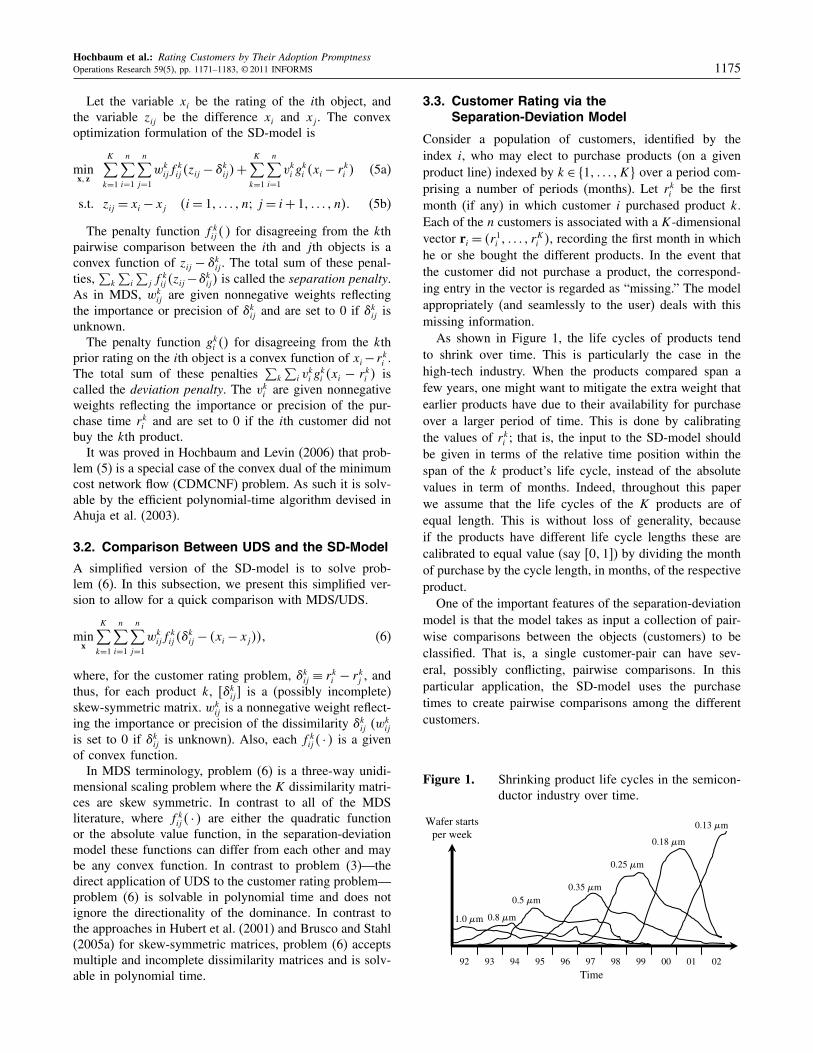
Rating the customers’ adoption promptness is partic-ularly important in high tech markets, where productsgenerally have short—and indeed shrinking—life cycles

(Talluri et al. 1998). For example, whereas memory semi-conductor chips had a life of mature product lasting approx-imately five years in the early 90s, this had shrunk to oneyear in the early 2000s, (see, e.g., Figure 1 for product lifecycles in the semiconductor industry).

The motivation of this paper is to solve the customerrating problem: Given data on a set of customers, a set ofproducts on a given product line, and the purchase times ofeach customer-product pair, the customer rating problem isto rate each customer according to his/her adoption prompt-ness. The proposed methodology is illustrated for commer-cial data from Sun Microsystems by rating the adoptionpromptness of some of their customers.

Our focus is on the customer rating problem where theinformation available is incomplete; that is, there are cus-tomers who do not purchase every product. This incompleteinformation scenario is a feature of the Sun database andit is typical for other companies, as well, that not all cus-tomers buy every product.

The customer rating problem is addressed here withHochbaum’s separation-deviation model (Hochbaum 2004),which has previously been used in contexts such as groupdecision making (Hochbaum and Levin 2006) and country-credit risk rating (Hochbaum and Moreno-Centeno 2008).This optimization model aims to minimize the sum of the

1171

Hochbaum et al.: Rating Customers by Their Adoption Promptness1172 Operations Research 59(5), pp. 1171–1183, © 2011 INFORMS

penalties on deviating from priors and from pairwise com-parisons. In the customer rating context, the priors arethe customers’ product purchase timings, and the pairwisecomparisons are derived from the relative difference in tim-ing of customers’ product purchases. The model is effi-ciently solvable, resulting in a scalar value for each cus-tomer representing their overall score of adoption prompt-ness. Note that the adoption behavior of customers usu-ally differs over different lines of products. Therefore, animportant assumption of the model is the homogeneity ofthe studied products. That is, the model assumes that theproducts belong to the same product line, and thus thecustomers have similar adoption behavior on the studiedproducts. (Even under this assumption, different productsare likely to indicate different timings and pairwise com-parisons.) Under this assumption, it is appropriate to givea single rating for each customer; this rating indicates thepromptness to adopt a new product on this particular prod-uct line.

Two of the main contributions of this paper are(1) applying Hochbaum’s separation-deviation model tothe customer rating problem and (2) reinterpreting theseparation-deviation model as a unidimensional scalingtechnique, thus presenting the model as an alternative towell-known dimension-reduction methodologies (in the spe-cial case where the data needs to be represented/summarizedin only one dimension), including unidimensional scal-ing, principal component analysis, factor analysis, andaveraging.

This paper is organized as follows. Section 2 reviewshow the customer rating problem has been previouslyaddressed in the literature and reviews several scaling anddimension-reduction methodologies that can be appliedto solve the customer rating problem. Section 3 reviewsthe separation-deviation model (hereafter referred to asSD-model) and indicates how the SD-model differs fromother techniques. Section 4 compares, in simulated scenar-ios, the performance of the SD-model to that of unidimen-sional scaling. Specifically, §4 compares the performanceof the two methods in simulated scenarios where the correctadoption promptness of the customers is known in advance.Section 5 presents a study on commercial data from SunMicrosystems and reports the generated insights obtainedby using our approach. Finally §6 gives some final remarksabout the SD-model and its usefulness for other types ofapplications.

2. Literature ReviewIn general, the input to data-mining techniques consists ofa collection of records that characterize customer purchasebehavior, as well as other relevant customer characteris-tics such as age, gender, usage rate, loyalty status, etc. Atan abstract level, many data-mining techniques attempt toexplain customer behavior in terms of a meaningful subsetof customer characteristics by identifying a function thatmaps a vector of customer attributes to a scalar value.

There are two main classes of data-mining techniques:those for supervised learning and those for unsupervisedlearning. The main objective of supervised learning tech-niques is to try to identify how to use independent vari-ables (i.e., observable customer characteristics) to be ableto predict an unobservable customer characteristic. Thesetechniques require as input a customer database with pre-classified customers. Some classical customer segmenta-tion techniques that fall under this category are auto-matic interaction detector (AID) and its extensions (e.g.,CHAID), linear regression and its generalizations (e.g.,canonical analysis), discriminant analysis, conjoint analy-sis and its extensions (e.g., componential segmentation andPOSSE—product optimization and selected segment evalu-ation), logistic regression, neural networks, etc. For the SunMicrosystems study we have no a priori labeling of the cus-tomers, i.e., we do not have a “training set.” Therefore, thefocus of this paper is on the unsupervised-learning problemof rating customers according to their adoption promptness.

In unsupervised-learning techniques, there is no preclas-sified set of customers. Thus, the unsupervised-learningtechniques aim to determine the customer ratings fromthe unlabeled data. Unsupervised-learning techniques canbe classified as cluster-analysis or dimension-reductiontechniques.

Cluster-analysis techniques solve the following problem:Given a data set containing information about n objects,cluster these objects into groups, such that objectsbelonging to the same cluster are similar in some sense.Cluster-analysis methods such as K-means, hierarchicalclustering, and Gaussian mixture models find a partition ofthe objects, so that the objects on each subset (cluster) sharea common trait. We mention a clustering approach, basedon maximum-cut clustering, for the customer segmentationproblem (Rusmevichientong et al. 2004). Maximum-cut isan NP-hard problem, so the approach in Rusmevichientonget al. (2004) is to approximate maximum-cut with semidef-inite programming. The output is not a full customer rating,but rather a classification of the customers only in earlyversus late adopters. We cannot compare directly cluster-ing techniques to the scaling methodology proposed in thispaper because the outputs are different. In particular, clus-tering techniques output a partition of the customers intoclusters, whereas our methodology assigns a rating to eachcustomer. Therefore we decided to compare our methodol-ogy with dimension-reduction techniques, whose output isstraightforwardly comparable to that of our methodology.

Dimension-reduction techniques (DRTs) solve the fol-lowing problem: Given an n× k matrix, R, find the n× k′

matrix with k′ < k that best captures the content in theoriginal matrix, according to a certain criterion. In the cus-tomer segmentation problem, R is the matrix containing thepurchase times of k products by n customers, and the out-put is an n× 1 vector that captures the relative “purchaseordering” of the customers. Some of the most widely used

Hochbaum et al.: Rating Customers by Their Adoption PromptnessOperations Research 59(5), pp. 1171–1183, © 2011 INFORMS 1173

DRTs are principal component analysis (PCA), factor anal-ysis (FA), multidimensional scaling (MDS), and averaging.We give (below) a brief description of each technique. Foran in-depth discussion of PCA, FA, and MDS, we referthe reader to Jollife (1986), Rummel (1970), and Torgerson(1952), respectively.

In essence, PCA seeks to reduce the dimension ofthe data by finding a few orthogonal linear combinations(the principal components) of the original variables withthe largest variance. The first principal component is thelinear combination with the largest variance; in this sense,it is the one-dimensional vector that best captures the infor-mation contained in the original data.

Factor analysis assumes that the measured variablesdepend on some unknown, and often unmeasurable, com-mon factors. The goal of FA is to uncover such relations.Typical examples include variables defined as various testscores of individuals, because such scores are thought to berelated to a common “intelligence” factor. Here the mea-sured variables are the purchase times of a customer, andthe unmeasurable factor of interest is the customer’s pro-clivity for early adoption.

Given n items in a k-dimensional space and an n × nmatrix of distances among the items, MDS produces ak′-dimensional, k′ < k, representation of the items such thatthe pairwise distances among the n points in the new spaceare similar to the distances in the original data.

The customer rating problem can also be addressed bythe (naive) DRT of the averaging method. Given a set ofpurchase times for customer i of product k, rki , the rat-ing obtained by the averaging method is given by x

avgi =

4∑

k∈Rirki 5/4�Ri�5, where Ri is the set of products purchased

by the ith customer.For most DRTs, including PCA and FA, missing data

pose serious problems (see Kosobud 1963, Afifi andElashoff 1966, for example). In the customer rating prob-lem, assuming full data is equivalent to assuming that allcustomers purchased every product. As discussed in §1,this does not hold in general, and in particular it does nothold for Sun’s data. These DRTs, PCA, and FA require thatthe missing values are estimated and artificially imputed.(In statistics, imputation is the substitution of some valuefor a missing data point or a missing component of a datapoint.) In contrast, modern versions of MDS (thoroughlyreviewed below) are designed specifically to handle missingdata without the need of imputation. Although modern ver-sions of PCA and FA versions do, in some sense, work onimputed values as well, they require that the imputed valuesare consistent with an underlying stochastic model for thedata. In the problem herein considered, there is not enoughdata to fit an underlying stochastic model. Thus, to be ableto use PCA and FA to solve our problem, we imputed themissing values using a simple nearest-neighbor missing-data-recovery method. Although this imputation methodhas been shown to be appropriate in the treatment of miss-ing data (Huang and Zhu 2002, Hruschka et al. 2003), this

was not the case in our study. Specifically, when using PCAand FA on the imputed data to solve our problem, their per-formances were dominated by those of the SD-model andMDS. (We note that there might be other imputation meth-ods that could potentially lead to better results.) Therefore,we will only present (in §4) the comparison of the perfor-mances of SD-model to MDS. Because the performanceof the average method was also dominated by that of theSD-model and MDS, we decided also not to include sucha performance comparison.

2.1. Review of Multidimensional Scaling

Multidimensional scaling (MDS) is a set of relatedtechniques used for representing the similarities anddissimilarities among pairs of objects as distances betweenpoints on a low-dimensional space. MDS models aim toapproximate given nonnegative dissimilarities, �ij , amongpairs of objects, i, j , by distances between points inan m-dimensional MDS configuration X. Here X, theconfiguration, is an n × m matrix with the coordinates ofthe n objects in <m. Most MDS techniques assume thatthe dissimilarity matrix 6�ij 7 is symmetric; we review twoimportant exceptions below. The most common function tomeasure the fit between the given dissimilarities, �ij , anddistances, dij4X5, is STRESS, defined by

STRESS4X5≡

n∑

i=1

n∑

j=1

wij4�ij −dij4X5521 (1)

where wij is a given nonnegative weight reflecting theimportance or precision of the dissimilarity �ij . Note thatwij can be set to 0 if �ij is unknown. dij4X5 is a vectornorm, defined as

dij4X5=

[ m∑

s=1

�xis − xjs�q

]1/q

with given parameter q ¾ 1. Usually, dij4X5 is the L2 norm4q = 25 or the L1 norm (q = 1).

Finding a global minimum of (1) is a hard optimizationproblem because STRESS is a nonlinear nonconvex func-tion with respect to X, and thus optimization algorithmscan converge to local minima (see, for example, de Leeuw1977, Groenen et al. 1999, Alexander et al. 2005).

In a useful MDS technique, the three-way MDS, for eachpair of objects we are given K dissimilarity measures fromdifferent “replications” (e.g., repeated measures, differentexperimental conditions, multiple raters, etc.). This tech-nique is referred to as three-way MDS because the inputis a three-dimensional matrix �k

ij , as opposed to the two-dimensional matrix in “classic” MDS. The objective func-tion of three-way MDS is defined as (de Leeuw 1977),

3WAY-STRESS4X5≡

K∑

k=1

n∑

i=1

n∑

j=1

wkij4�

kij −dij4X5520 (2)


Unidimensional scaling (UDS) is the important one-dimensional case of MDS where the configuration X is ann × 1 matrix. Therefore, UDS seeks to approximate thegiven dissimilarities by distances between points in a one-dimensional space. Unidimensional scaling has been usedsuccessfully in several contexts (see, for example, Fisher1922, Robinson 1951, Ge et al. 2005). Unidimensional scal-ing has been studied mainly as a model for object sequenc-ing and seriation (Hubert et al. 2001, Brusco and Stahl2005b), thus its relevance to the problem concerning thispaper. Unidimensional scaling is a hard optimization prob-lem, and combinatorial techniques (e.g., branch and boundand dynamic programming) are only able to optimally solveinstances of up to 30 objects; see, for example, Lau et al.(1998), Brusco (2002), Hubert et al. (2002), Brusco andStahl (2005c).

In our particular application, rating customers accordingto their adoption promptness, the input data is a matrix Rwith rki giving the adoption time (relative to product launch)of customer i for product k. This matrix is, in general,incomplete and has many missing elements. The objectiveis to assign each customer i to a scale x such that xi mostaccurately recovers the across-customer ordering of productadoption times within any product. To solve our problem,we can set up the following three-way UDS problem:

minx

K∑

k=1

n∑

i=1

n∑

j=1

wkij4�r

ki − rkj � − �xi − xj �5

20 (3)

Here the interpretation is that product k gives a pairwisedissimilarity, �rki − rkj �, among a pair of customers i andj the purchased product k. Then, the objective is that cus-tomers with low (high) dissimilarities have similar (dissim-ilar) adoption promptness and should be placed “close (far)to each other” in the desired scale x.

We note a couple of drawbacks of formulating ourcustomer rating problem as the three-way UDS prob-lem (3), and later introduce our scaling methodologywhich, addresses these drawbacks.

1. As mentioned earlier, finding the optimal solutionto (3) is a hard optimization problem because the objectiveis nonconvex (Groenen et al. 1999); current optimizationtechniques are only able to optimally solve instances of atmost 30 objects.

2. By calculating the dissimilarities as �rki − rkj �, prob-lem (3) ignores the so-called directionality of dominance,that is, the sign of 4rki − rkj 5. In particular, problem (3)does not capture the information regarding which customeradopted product k earlier. Note that this information is veryrelevant in the customer rating problem.

A closely related observation is that, given an optimalsolution, x∗, to (3), −x∗ is also an optimal solution to (3).Thus, by solving (3), we get a rating of the customers, butwe do not know whether a higher rating means a greateradoption promptness or vice versa.

Although the vast majority of the papers in the UDS lit-erature assume that the given dissimilarities are nonnegative

and symmetric, there are two papers (Hubert et al. 2001and Brusco and Stahl 2005a) that consider the case wherethe dissimilarities are given in a complete skew-symmetricmatrix (i.e., �ij = −�ji).

Because these approaches consider only one matrix 6�ij 7and this matrix is complete, these are not applicable tothe customer rating problem. Indeed, the approach pre-sented in this paper is a nice generalization of one of theseapproaches. We briefly discuss the approaches presented inHubert et al. (2001) and Brusco and Stahl (2005a) and referto the original papers for further details.

Hubert et al. (2001) observe that a skew-symmetricmatrix contains two distinct types of information betweenany pair of objects: degree of dissimilarity, ��ij �, anddirectionality of dominance, sign4�ij5. They consider twoapproaches to sequencing the objects. The first approachconsists of finding the object ordering � such that thematrix 6��4i5�4j57 has the maximum sum of above-diagonalentries. Hubert et al. note that this problem is exactly theminimum feedback arc set problem, which is NP-hard. Thesecond approach proposed in Hubert et al. (2001) is to solvethe following problem,

minx

n∑

i=1

n∑

j=1

4�ij − 4xi − xj5521 (4)

where the dissimilarity matrix 6�ij 7 is assumed to be skewsymmetric and has no missing entries. Hubert et al. give ananalytic solution to problem (4); Hochbaum and Moreno-Centeno (2008) give a generalization of this result to thecase of multiple dissimilarity matrices (but still no missingentries).

Brusco and Stahl (2005a) also differentiate between thedegree of dissimilarity, ��ij �, and directionality of dom-inance, sign4�ij5. They propose a bicriteria optimizationproblem that balances between these two types of infor-mation. Although interesting, this approach is not practi-cal because the proposed solution technique is only ableto determine the nondominated solutions for matrices upto size 20 × 20 (and can take as input only one skew-symmetric matrix).

3. The Separation-Deviation Model

3.1. Review of the Separation-Deviation Model

The SD-model was proposed by Hochbaum (2004, 2006).The inputs for the separation-deviation model are a set ofobjects 811 0 0 0 1 n9, for each object a set of prior ratingsrki for k = 1 0 0 0K, and a set of pairwise comparisons �k

ij

for k = 1 0 0 0K for each pair of objects. These pairwisecomparisons are skew-symmetric, that is �k

ij = −�kji. The

SD-model aims to assign each object a rating xi, such thatxi is as close as possible to the given prior ratings and thedifference in the ratings of each pair of objects is as closeas possible to the given pairwise comparisons.


Let the variable xi be the rating of the ith object, andthe variable zij be the difference xi and xj . The convexoptimization formulation of the SD-model is

minx1 z

K∑

k=1

n∑

i=1

n∑

j=1

wkijf

kij 4zij − �k

ij5+

K∑

k=1

n∑

i=1

vki gki 4xi − rki 5 (5a)

s.t. zij = xi − xj 4i = 11 0 0 0 1 n3 j = i+ 11 0 0 0 1 n50 (5b)

The penalty function f kij 4 5 for disagreeing from the kth

pairwise comparison between the ith and jth objects is aconvex function of zij − �k

ij . The total sum of these penal-ties,

∑

k

∑

i

∑

j fkij 4zij −�k

ij5 is called the separation penalty.As in MDS, wk

ij are given nonnegative weights reflectingthe importance or precision of �k

ij and are set to 0 if �kij is

unknown.The penalty function gki 45 for disagreeing from the kth

prior rating on the ith object is a convex function of xi −rki .The total sum of these penalties

∑

k

∑

i vki g

ki 4xi − rki 5 is

called the deviation penalty. The vki are given nonnegativeweights reflecting the importance or precision of the pur-chase time rki and are set to 0 if the ith customer did notbuy the kth product.

It was proved in Hochbaum and Levin (2006) that prob-lem (5) is a special case of the convex dual of the minimumcost network flow (CDMCNF) problem. As such it is solv-able by the efficient polynomial-time algorithm devised inAhuja et al. (2003).

3.2. Comparison Between UDS and the SD-Model

A simplified version of the SD-model is to solve prob-lem (6). In this subsection, we present this simplified ver-sion to allow for a quick comparison with MDS/UDS.

minx

K∑

k=1

n∑

i=1

n∑

j=1

wkijf

kij 4�

kij − 4xi − xj551 (6)

where, for the customer rating problem, �kij ≡ rki − rkj , and

thus, for each product k, 6�kij 7 is a (possibly incomplete)

skew-symmetric matrix. wkij is a nonnegative weight reflect-

ing the importance or precision of the dissimilarity �kij (wk

ij

is set to 0 if �kij is unknown). Also, each f k

ij 4 · 5 is a givenof convex function.

In MDS terminology, problem (6) is a three-way unidi-mensional scaling problem where the K dissimilarity matri-ces are skew symmetric. In contrast to all of the MDSliterature, where f k

ij 4 · 5 are either the quadratic functionor the absolute value function, in the separation-deviationmodel these functions can differ from each other and maybe any convex function. In contrast to problem (3)—thedirect application of UDS to the customer rating problem—problem (6) is solvable in polynomial time and does notignore the directionality of the dominance. In contrast tothe approaches in Hubert et al. (2001) and Brusco and Stahl(2005a) for skew-symmetric matrices, problem (6) acceptsmultiple and incomplete dissimilarity matrices and is solv-able in polynomial time.

3.3. Customer Rating via theSeparation-Deviation Model

Consider a population of customers, identified by theindex i, who may elect to purchase products (on a givenproduct line) indexed by k ∈ 811 0 0 0 1K9 over a period com-prising a number of periods (months). Let rki be the firstmonth (if any) in which customer i purchased product k.Each of the n customers is associated with a K-dimensionalvector ri = 4r1

i 1 0 0 0 1 rKi 5, recording the first month in which

he or she bought the different products. In the event thatthe customer did not purchase a product, the correspond-ing entry in the vector is regarded as “missing.” The modelappropriately (and seamlessly to the user) deals with thismissing information.

As shown in Figure 1, the life cycles of products tendto shrink over time. This is particularly the case in thehigh-tech industry. When the products compared span afew years, one might want to mitigate the extra weight thatearlier products have due to their availability for purchaseover a larger period of time. This is done by calibratingthe values of rki ; that is, the input to the SD-model shouldbe given in terms of the relative time position within thespan of the k product’s life cycle, instead of the absolutevalues in term of months. Indeed, throughout this paperwe assume that the life cycles of the K products are ofequal length. This is without loss of generality, becauseif the products have different life cycle lengths these arecalibrated to equal value (say 60117) by dividing the monthof purchase by the cycle length, in months, of the respectiveproduct.

One of the important features of the separation-deviationmodel is that the model takes as input a collection of pair-wise comparisons between the objects (customers) to beclassified. That is, a single customer-pair can have sev-eral, possibly conflicting, pairwise comparisons. In thisparticular application, the SD-model uses the purchasetimes to create pairwise comparisons among the differentcustomers.

Figure 1. Shrinking product life cycles in the semicon-ductor industry over time.

Wafer startsper week

0201009998979695949392

1.0 �m 0.8 �m

0.5 �m0.35 �m

0.25 �m

0.18 �m

0.13 �m

Time


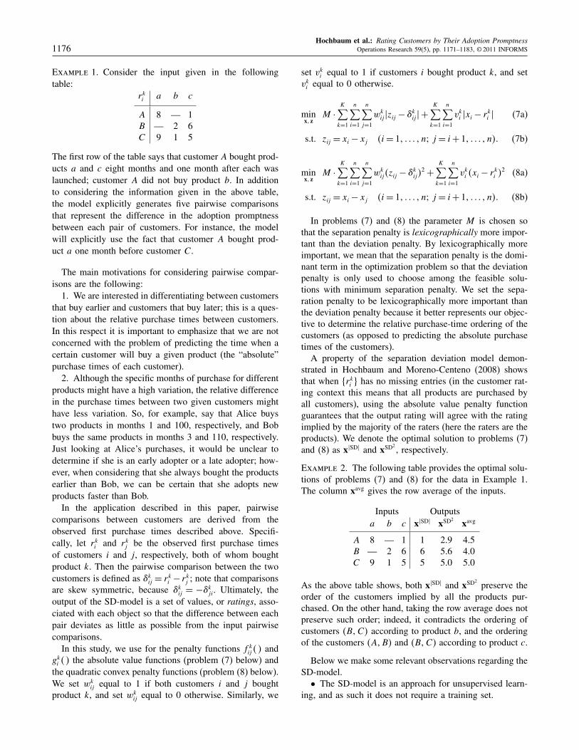
Example 1. Consider the input given in the followingtable:

rki a b c

A 8 — 1B — 2 6C 9 1 5

The first row of the table says that customer A bought prod-ucts a and c eight months and one month after each waslaunched; customer A did not buy product b. In additionto considering the information given in the above table,the model explicitly generates five pairwise comparisonsthat represent the difference in the adoption promptnessbetween each pair of customers. For instance, the modelwill explicitly use the fact that customer A bought prod-uct a one month before customer C.

The main motivations for considering pairwise compar-isons are the following:

1. We are interested in differentiating between customersthat buy earlier and customers that buy later; this is a ques-tion about the relative purchase times between customers.In this respect it is important to emphasize that we are notconcerned with the problem of predicting the time when acertain customer will buy a given product (the “absolute”purchase times of each customer).

2. Although the specific months of purchase for differentproducts might have a high variation, the relative differencein the purchase times between two given customers mighthave less variation. So, for example, say that Alice buystwo products in months 1 and 100, respectively, and Bobbuys the same products in months 3 and 110, respectively.Just looking at Alice’s purchases, it would be unclear todetermine if she is an early adopter or a late adopter; how-ever, when considering that she always bought the productsearlier than Bob, we can be certain that she adopts newproducts faster than Bob.

In the application described in this paper, pairwisecomparisons between customers are derived from theobserved first purchase times described above. Specifi-cally, let rki and rkj be the observed first purchase timesof customers i and j , respectively, both of whom boughtproduct k. Then the pairwise comparison between the twocustomers is defined as �k

ij = rki − rkj ; note that comparisonsare skew symmetric, because �k

ij = −�kji. Ultimately, the

output of the SD-model is a set of values, or ratings, asso-ciated with each object so that the difference between eachpair deviates as little as possible from the input pairwisecomparisons.

In this study, we use for the penalty functions f kij 4 5 and

gki 4 5 the absolute value functions (problem (7) below) andthe quadratic convex penalty functions (problem (8) below).We set wk

ij equal to 1 if both customers i and j boughtproduct k, and set wk

ij equal to 0 otherwise. Similarly, we

set vki equal to 1 if customers i bought product k, and setvki equal to 0 otherwise.

minx1 z

M ·

K∑

k=1

n∑

i=1

n∑

j=1

wkij �zij − �k

ij � +

K∑

k=1

n∑

i=1

vki �xi − rki � (7a)


minx1 z

M ·

K∑

k=1

n∑

i=1

n∑

j=1

wkij4zij − �k

ij52+

K∑

k=1

n∑

i=1

vki 4xi − rki 52 (8a)


In problems (7) and (8) the parameter M is chosen sothat the separation penalty is lexicographically more impor-tant than the deviation penalty. By lexicographically moreimportant, we mean that the separation penalty is the domi-nant term in the optimization problem so that the deviationpenalty is only used to choose among the feasible solu-tions with minimum separation penalty. We set the sepa-ration penalty to be lexicographically more important thanthe deviation penalty because it better represents our objec-tive to determine the relative purchase-time ordering of thecustomers (as opposed to predicting the absolute purchasetimes of the customers).

A property of the separation deviation model demon-strated in Hochbaum and Moreno-Centeno (2008) showsthat when 8rki 9 has no missing entries (in the customer rat-ing context this means that all products are purchased byall customers), using the absolute value penalty functionguarantees that the output rating will agree with the ratingimplied by the majority of the raters (here the raters are theproducts). We denote the optimal solution to problems (7)and (8) as x�SD� and xSD2

, respectively.

Example 2. The following table provides the optimal solu-tions of problems (7) and (8) for the data in Example 1.The column xavg gives the row average of the inputs.

Inputs Outputsa b c x�SD� xSD2

xavg

A 8 — 1 1 2.9 4.5B — 2 6 6 5.6 4.0C 9 1 5 5 5.0 5.0

As the above table shows, both x�SD� and xSD2preserve the

order of the customers implied by all the products pur-chased. On the other hand, taking the row average does notpreserve such order; indeed, it contradicts the ordering ofcustomers 4B1C5 according to product b, and the orderingof the customers 4A1B5 and 4B1C5 according to product c.

Below we make some relevant observations regarding theSD-model.

• The SD-model is an approach for unsupervised learn-ing, and as such it does not require a training set.


• A particular advantage of the SD-model is that in addi-tion to working well in situations with complete informa-tion (see Hochbaum and Moreno-Centeno 2008), it workswell (without any need for data preprocessing) in situationswhere we have incomplete information. This is particularlyprominent in the application studied here, where the infor-mation matrix is sparse. Indeed, in the Sun Microsystemsdatabase, only 165 of 1,916 customers bought all the prod-ucts considered in this study, and 1,132 customers onlybought one product.

• The SD-model can take subjective, or less thanentirely reliable, judgments as input and calibrate thoseinputs with appropriate confidence levels.

• The SD-model is solvable in polynomial time for anyconvex penalty functions f k

ij 4 5 and gki 4 5.• The segmentation achieved by the SD-model is the

“best” according to a defined metric.• The SD-model makes obvious the discrepancies that

exist between the inputs. Outliers are made explicit andmay be used to improve insights into customer behavior. Inparticular, by identifying the highest penalty terms one candetect outliers in both the pairwise comparisons and in theprior ratings.

• The SD-model does not rely on specified distributionsfor different classes, and there is no requirement of anyspecific sample size.

4. Performance Assessment onSimulated Scenarios

This section assesses the performance of the SD-modelunder several different simulated scenarios and comparesits performance to that of three-way UDS (problem (3)).

We denote as xUDS the customer rating obtained usingthree-way UDS, that is, the solution to problem (3). Recallthat obtaining the optimal solution to problem (3) is onlypossible (with current optimization techniques) for n¶ 30(Hubert et al. 2001). Although specialized heuristics tosolve UDS are available (Hubert et al. 2002 survey theseheuristics), none of them apply to the three-way UDS or tothe weighted UDS (that is, all of the heuristics assume thatthe data is complete and wij = 1 for i1 j = 11 0 0 0 1 n). There-fore to find a heuristic solution to problem (3), we usedMatlab’s heuristic to solve the weighted MDS problem.Strictly speaking, Matlab’s heuristic was designed to min-imize problem (1) (that is, it only accepts one dissimilar-ity matrix). However, as shown in de Leeuw (1977), whenusing the quadratic function as penalty function, minimiz-ing (2) can be reduced to the problem of minimizing (1).

Each scenario represents a different customer purchase-timing behavior and consists of 600 customers each buyingup to four products. We associate a different purchase-timedistribution with each customer-product pair. By letting thepurchase-time distributions depend on both the customerand the product, we are able to simulate scenarios wherethe products have different life cycles and characteristics.

In these scenarios, the customers’ purchase times may havedifferent expected values and/or variances depending on theproduct under consideration.

We simulated the purchase time of each product byeach customer using the gamma distribution, which is com-monly used to simulate “customer arrival times.” Let c andp represent the index of the customer and product, respec-tively. We used seven different expected purchase times8c1 c+ 2p1 c + 5p1 c + 50p1 cp110cp150cp9, and 11 dif-ferent variances 81015015c110c150c15p110p150p15c +

5p110c+10p150c+50p9. Overall, we simulated 77 differ-ence scenarios, one for each possible mean-variance com-bination. For example, in the scenario having cp mean and5p + 5c variance, the purchase time of the jth product bythe ith customer had an expected value of ij and a varianceof 5i + 5j . Note that in all of these scenarios, customerswith lower indices adopt new products earlier. That is, giventwo customers i, j such that i < j , then, for any given prod-uct, customer i has an earlier expected purchase time thancustomer j . Thus, for every one of the 77 scenarios, thecustomers are ordered with respect to their adoption prompt-ness. In particular, the true ranking, xT

i , of the ith customeris equal to i. Note that the simulated customers behave sim-ilarly across products in that lower-index customers adopt(in expected value) earlier than higher-index customers forany given product; this is consistent with the assumptionthat all the products belong to the same product line.

To measure how successful the SD-model is in recov-ering the true ranking vector, xT, of the customers, weused Kendall’s Tau rank-correlation coefficient. This coef-ficient provides a measure of the degree of correspondencebetween two vectors. In particular, it assesses how well theorder (i.e., rank) of the elements of the vectors is preserved.In Appendix A we provide a description of Kendall’s Taurank-correlation coefficient. We note that, as an alternativeto three-way UDS (problem (3) and the SD model (prob-lems (7) and (8)), we could instead find the customer ratingvector that maximizes Kendall’s Tau rank-correlation coef-ficient. We decided not to do so because (1) finding sucha vector is NP-hard (Bartholdi et al. 1989) and (2) thisobjective would ignore the degree of dissimilarity betweenthe adoption times of the customers. On the other hand,we believe that Kendall’s Tau rank-correlation coefficientis appropriate to measure how well the customer ratingsrecovered xT

i . (Notice that xTi gives the true ordering of

the customers and does not give a degree of dissimilaritybetween the customers.)

Recall that this paper focuses on the case where the dataavailable is incomplete; that is, there are customers who didnot purchase every product. To generate incomplete data,we first simulated the complete data; that is, we simulatedthe purchase times of every customer-product pair and thendeleted some of the purchase times at random. In Sun’sdata 59%, 23%, 9%, and 9% of the customers bought one,two, three, and four products, respectively. We mimicked


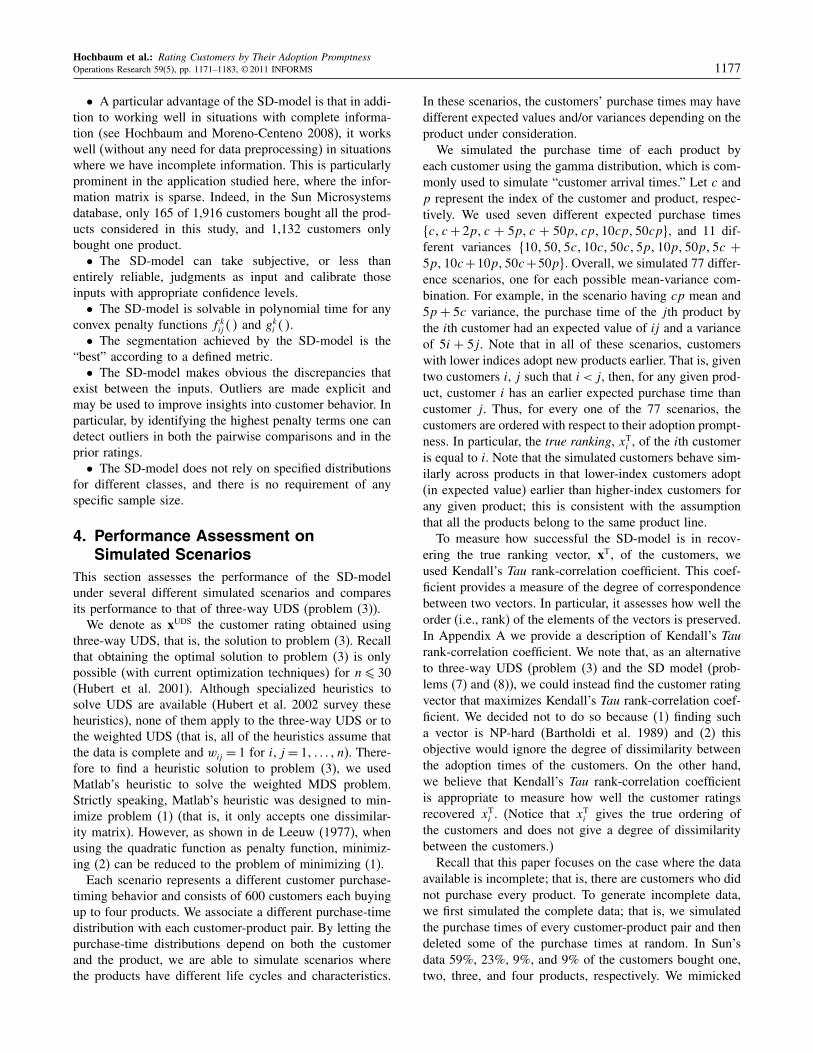
Table 1. Average Tau correlation coefficients between xT and x�SD�.

� 10 50 5c 10c 50c 5p 10p 50p 5c + 5p 10c + 10p 50c + 50p

c 009913 009784 008884 008434 006934 009902 009857 009662 008873 008433 006903c + 2p 009911 009783 008872 008445 006947 009903 009855 009666 008879 008450 006903c + 5p 009912 009785 008886 008455 006900 009905 009856 009666 008851 008444 006906c + 50p 009913 009784 008877 008448 006847 009904 009856 009665 008863 008430 006830cp 008427 008386 008271 008198 007745 008395 008416 008428 008270 008161 00776610cp 008431 008449 008432 008419 008403 008439 008424 008441 008438 008426 00839150cp 008426 008443 008433 008437 008452 008437 008433 008438 008451 008462 008423

this data by deleting the entries with this empirical distribu-tion. In particular, each customer had a probability of 0.59,0.23, 0.09, and 0.09 of buying one, two, three, and fourproducts. For each customer the purchased products werechosen uniformly at random.

To summarize, the performance assessment of the SD-model on each of the 77 scenarios was executed as follows:

Step 1: Repeat 30 times:Step 1.1: Simulate the purchase-time data of four

products by 600 customers.Step 1.2: Delete some of the purchase times at ran-

dom to obtain incomplete information.Step 1.3: Solve for x�SD�, xSD2

, and xUDS.Step 1.4: Compute the Tau correlation coefficient

between xT (the true customer ranking) and each of x�SD�,xSD2

, and xUDS.Step 2: Calculate the average and standard deviation of

the 30 Tau correlation coefficients (with xT) computed foreach of x�SD�, xSD2

, and xUDS.Tables 1–3 give, for each of the 77 scenarios, the average

Tau correlation coefficient between xT and x�SD�, xSD2, and

xUDS, respectively.To compare the performances of these methods,

Tables 4–6 provide the average differences between the

Table 2. Average Tau correlation coefficients between xT and xSD2.

� 10 50 5c 10c 50c 5p 10p 50p 5c + 5p 10c + 10p 50c + 50p

c 009915 009788 008903 008464 006958 009902 009858 009660 008891 008453 006928c + 2p 009913 009787 008891 008468 006971 009902 009856 009666 008897 008474 006936c + 5p 009914 009788 008904 008478 006925 009905 009856 009666 008873 008467 006932c + 50p 009915 009789 008902 008474 006892 009904 009857 009665 008882 008452 006871cp 008356 008322 008241 008169 007745 008333 008351 008365 008238 008140 00775810cp 008349 008380 008357 008350 008339 008360 008348 008371 008368 008360 00833150cp 008348 008373 008351 008366 008385 008362 008365 008368 008372 008383 008347

Table 3. Average Tau correlation coefficients between xT and xUDS.

� 10 50 5c 10c 50c 5p 10p 50p 5c + 5p 10c + 10p 50c+50p

c 009787 009781 009766 009767 007198 007618 007613 009708 009712 009710 009704c + 2p 007602 007697 007662 008871 008868 008879 008867 007610 007691 007645 008442c + 5p 008450 008450 008458 007583 007677 007662 006893 006917 006769 006842 007287c + 50p 007659 007678 009770 009782 009764 009756 007644 007664 007688 009764 009742cp 009739 009740 007624 007676 007668 009603 009599 009617 009612 007665 00768110cp 007674 008862 008874 008843 008854 007578 007150 007650 008443 008456 00843650cp 008433 007188 007171 007195 006856 006887 006886 006816 007305 007628 007651

correlation coefficients achieved by the different meth-ods. For example, each entry in Table 4 is the differencebetween the corresponding entries of Tables 1 and 3. InTables 4–6, the numbers given in bold are those that areat least three standard deviations above (or below) zero.Therefore the scenarios with bold entry are those whereone method significantly outperforms the other; whereas, inthe rest of the scenarios, the performance of both methodsis essentially the same.

The results in Tables 4 and 5 provide evidence that theSD-model, irrespective of the penalty functions used, per-forms better than UDS on most of the 77 scenarios. Inparticular, the SD-model outperforms UDS in 46 out of the77 scenarios; and in 36 of these 46 scenarios, the SD-modelsignificantly outperforms UDS.

We now compare the performance of the SD-modelusing different penalty functions. For this purpose, Table 6reports the average difference between the correlation coef-ficients (with respect to xT) for x�SD� and xSD2

. We note thatusing the absolute-value penalty functions is only slightlybetter than using the quadratic-value penalty functions.

The simulation results indicate that the SD-model deter-mines with high accuracy the true ranking of the customerswith respect to their adoption promptness.


Table 4. Average difference between the correlation coefficients obtained by x�SD� and xUDS.

� 10 50 5c 10c 50c 5p 10p 50p 5c + 5p 10c + 10p 50c + 50p

c 000126 000003 −000882 −001333 −000265 002283 002244 −000046 −000840 −001277 −002801c + 2p 002310 002087 001210 −000427 −001921 001024 000988 002056 001188 000805 −001539c + 5p 001462 001335 000427 000872 −000778 002243 002962 002748 002082 001603 −000381c + 50p 002254 002106 −000893 −001333 −002918 000148 002212 002000 001175 −001334 −002912cp −001312 −001354 000647 000522 000076 −001207 −001183 −001189 −001343 000496 00008510cp 000756 −000413 −000442 −000424 −000451 000861 001274 000792 −000005 −000030 −00004550cp −000007 001255 001262 001241 001596 001549 001547 001622 001145 000834 000773

Note. Positive numbers indicate that x�SD� has higher average correlation with xT than xUDS.

Table 5. Average difference between the correlation coefficients obtained by xSD2and xUDS.

� 10 50 5c 10c 50c 5p 10p 50p 5c + 5p 10c + 10p 50c + 50p

c 000128 000007 −000863 −001303 −000241 002283 002244 −000048 −000822 −001257 −002776c + 2p 002311 002090 001230 −000403 −001896 001024 000988 002056 001205 000829 −001506c + 5p 001464 001338 000445 000894 −000752 002243 002963 002749 002103 001626 −000356c + 50p 002256 002110 −000869 −001307 −002872 000148 002213 002000 001195 −001312 −002871cp −001383 −001417 000617 000493 000077 −001270 −001248 −001251 −001375 000475 00007710cp 000675 −000483 −000517 −000494 −000516 000782 001199 000721 −000075 −000096 −00010450cp −000085 001185 001179 001171 001529 001475 001479 001551 001067 000754 000696

Note. Positive numbers indicate that xSD2 has higher average correlation with xT than xUDS.

Table 6. Average difference between the correlation coefficients obtained by x�SD� and xSD2.

� 10 50 5c 10c 50c 5p 10p 50p 5c + 5p 10c + 10p 50c + 50p

c −000002 −000004 −000019 −000030 −000024 000000 −000001 000002 −000018 −000020 −000025c + 2p −000001 −000004 −000020 −000023 −000024 000000 000000 000000 −000017 −000024 −000033c + 5p −000002 −000003 −000018 −000022 −000026 000000 −000001 000000 −000021 −000023 −000026c + 50p −000002 −000004 −000024 −000026 −000045 000000 000000 000000 −000020 −000023 −000041cp 000071 000064 000030 000029 000000 000063 000065 000062 000032 000021 00000810cp 000081 000069 000075 000069 000064 000079 000075 000070 000070 000066 00005950cp 000078 000070 000082 000071 000067 000074 000068 000071 000079 000079 000077

Note. Positive numbers indicate that x�SD� has higher average correlation with xT than xSD2 .

5. Rating Sun’s Customers According toTheir Adoption Promptness

5.1. Sun’s Data

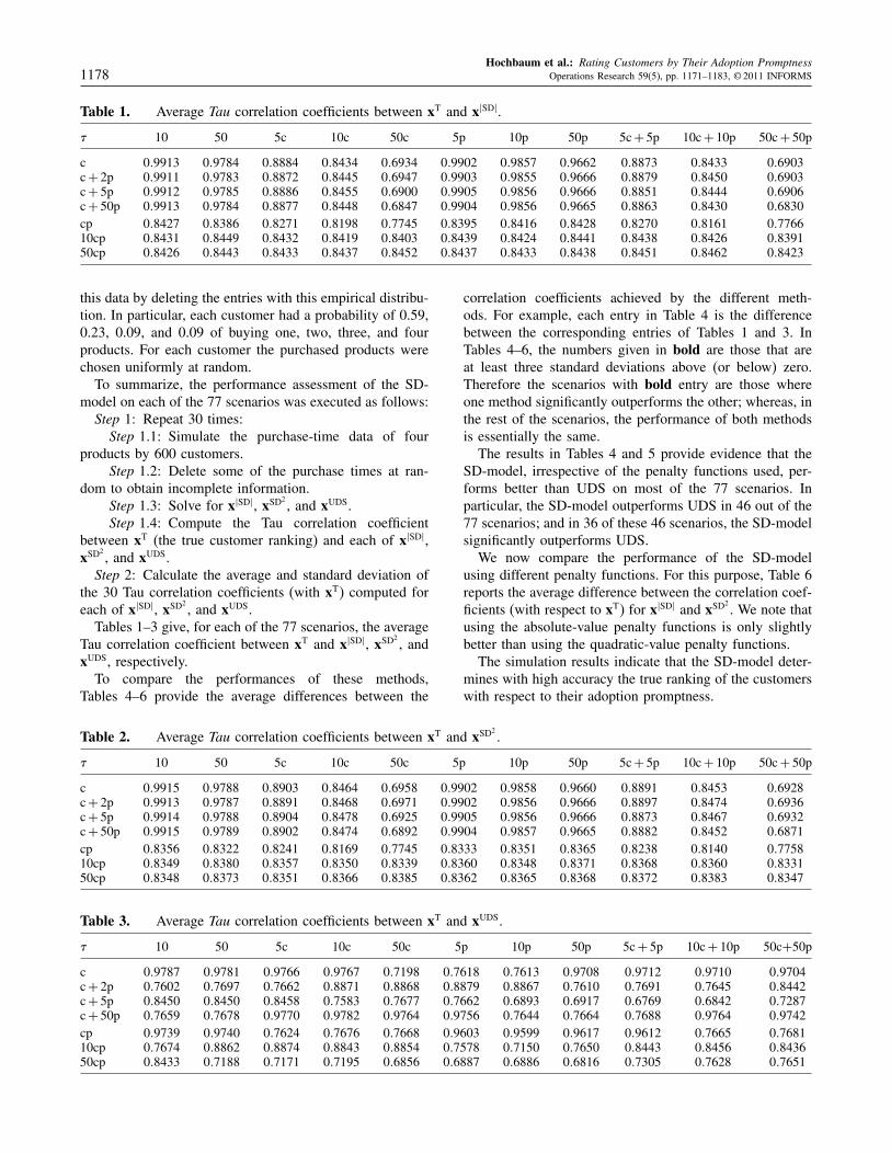
The empirical analysis presented below is based on a (dis-guised) data set comprising customer purchase informationprovided by Sun Microsystems, Inc. The data set encom-passes four products and some 1,916 customers. It recordsthe number of months (measured from the month of theearliest product launch) that elapsed before each customerbought each product. This section shows that Sun’s prod-ucts are not independent in several ways (for instance, allfour products are servers in the same family), and we pro-pose how to cope with this situation.

As shown in Figure 2, most of the customers did not buyall four products, and in fact about half of the customersonly bought one of the products. Such sparse data wouldpose a challenge for many of the existing data-mining andmarket segmentation techniques described in §2, and ingeneral, some form of preprocessing would be required to

fill in the missing data. The separation deviation model,however, handles missing data quite routinely, without pre-processing.

As may be deduced from Figure 3, products 3 and 4were launched together at the beginning of the observation

Figure 2. Number of customers that bought each prod-uct or set of products.

Product 4Product 1

Product 3Product 2

179171

586244

149652633

1655368

6253

55


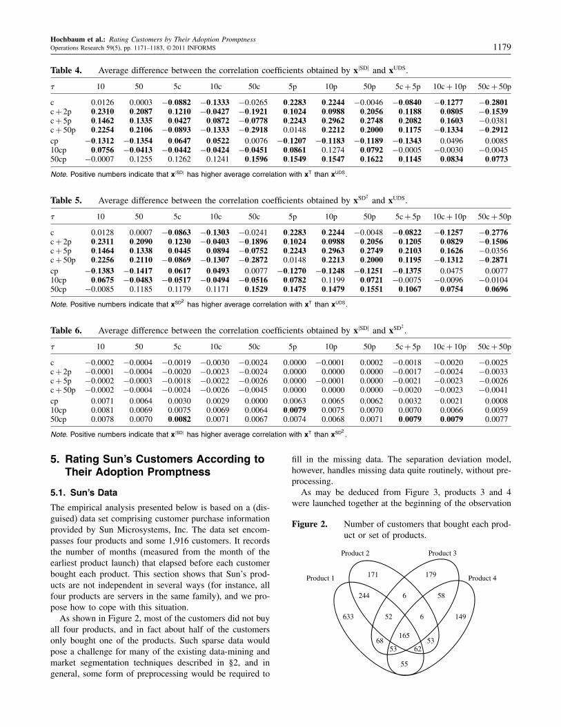
Figure 3. Number of customers that bought each prod-uct per month.

33312927252321191715131197531

Release time of products 3 and 4

140

120

100

80

60

40

20

0

Product 1Product 2Product 3Product 4

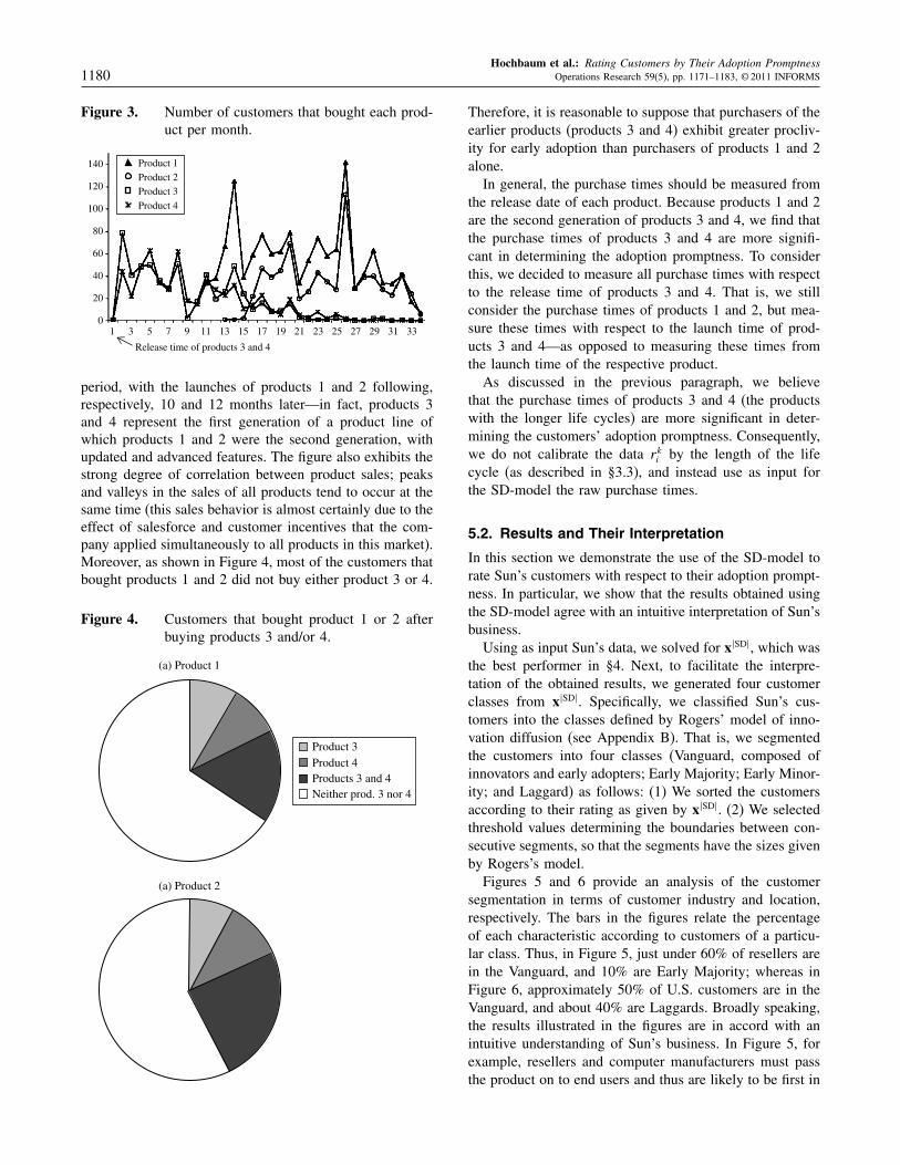
period, with the launches of products 1 and 2 following,respectively, 10 and 12 months later—in fact, products 3and 4 represent the first generation of a product line ofwhich products 1 and 2 were the second generation, withupdated and advanced features. The figure also exhibits thestrong degree of correlation between product sales; peaksand valleys in the sales of all products tend to occur at thesame time (this sales behavior is almost certainly due to theeffect of salesforce and customer incentives that the com-pany applied simultaneously to all products in this market).Moreover, as shown in Figure 4, most of the customers thatbought products 1 and 2 did not buy either product 3 or 4.

Figure 4. Customers that bought product 1 or 2 afterbuying products 3 and/or 4.

Product 3Product 4Products 3 and 4Neither prod. 3 nor 4

(a) Product 1

(a) Product 2

Therefore, it is reasonable to suppose that purchasers of theearlier products (products 3 and 4) exhibit greater procliv-ity for early adoption than purchasers of products 1 and 2alone.

In general, the purchase times should be measured fromthe release date of each product. Because products 1 and 2are the second generation of products 3 and 4, we find thatthe purchase times of products 3 and 4 are more signifi-cant in determining the adoption promptness. To considerthis, we decided to measure all purchase times with respectto the release time of products 3 and 4. That is, we stillconsider the purchase times of products 1 and 2, but mea-sure these times with respect to the launch time of prod-ucts 3 and 4—as opposed to measuring these times fromthe launch time of the respective product.

As discussed in the previous paragraph, we believethat the purchase times of products 3 and 4 (the productswith the longer life cycles) are more significant in deter-mining the customers’ adoption promptness. Consequently,we do not calibrate the data rki by the length of the lifecycle (as described in §3.3), and instead use as input forthe SD-model the raw purchase times.

5.2. Results and Their Interpretation

In this section we demonstrate the use of the SD-model torate Sun’s customers with respect to their adoption prompt-ness. In particular, we show that the results obtained usingthe SD-model agree with an intuitive interpretation of Sun’sbusiness.

Using as input Sun’s data, we solved for x�SD�, which wasthe best performer in §4. Next, to facilitate the interpre-tation of the obtained results, we generated four customerclasses from x�SD�. Specifically, we classified Sun’s cus-tomers into the classes defined by Rogers’ model of inno-vation diffusion (see Appendix B). That is, we segmentedthe customers into four classes (Vanguard, composed ofinnovators and early adopters; Early Majority; Early Minor-ity; and Laggard) as follows: (1) We sorted the customersaccording to their rating as given by x�SD�. (2) We selectedthreshold values determining the boundaries between con-secutive segments, so that the segments have the sizes givenby Rogers’s model.

Figures 5 and 6 provide an analysis of the customersegmentation in terms of customer industry and location,respectively. The bars in the figures relate the percentageof each characteristic according to customers of a particu-lar class. Thus, in Figure 5, just under 60% of resellers arein the Vanguard, and 10% are Early Majority; whereas inFigure 6, approximately 50% of U.S. customers are in theVanguard, and about 40% are Laggards. Broadly speaking,the results illustrated in the figures are in accord with anintuitive understanding of Sun’s business. In Figure 5, forexample, resellers and computer manufacturers must passthe product on to end users and thus are likely to be first in


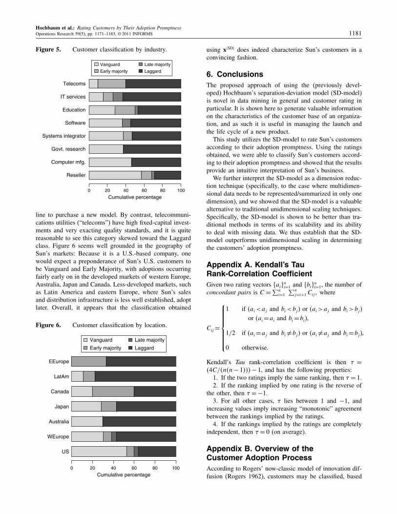
Figure 5. Customer classification by industry.

Reseller

Computer mfg.

Govt. research

Systems integrator

Software

Education

IT services

Telecoms

Cumulative percentage0 20 40 60 80 100

Vanguard

Early majority

Late majority

Laggard

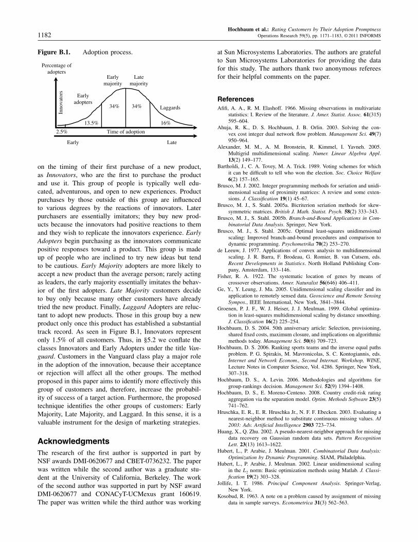
line to purchase a new model. By contrast, telecommuni-cations utilities (“telecoms”) have high fixed-capital invest-ments and very exacting quality standards, and it is quitereasonable to see this category skewed toward the Laggardclass. Figure 6 seems well grounded in the geography ofSun’s markets: Because it is a U.S.-based company, onewould expect a preponderance of Sun’s U.S. customers tobe Vanguard and Early Majority, with adoptions occurringfairly early on in the developed markets of western Europe,Australia, Japan and Canada. Less-developed markets, suchas Latin America and eastern Europe, where Sun’s salesand distribution infrastructure is less well established, adoptlater. Overall, it appears that the classification obtained

Figure 6. Customer classification by location.

US

WEurope

Australia

Japan

Canada

LatAm

EEurope

Cumulative percentage0 20 40 60 80 100

Vanguard

Early majority

Late majority

Laggard

using x�SD� does indeed characterize Sun’s customers in aconvincing fashion.

6. ConclusionsThe proposed approach of using the (previously devel-oped) Hochbaum’s separation-deviation model (SD-model)is novel in data mining in general and customer rating inparticular. It is shown here to generate valuable informationon the characteristics of the customer base of an organiza-tion, and as such it is useful in managing the launch andthe life cycle of a new product.

This study utilizes the SD-model to rate Sun’s customersaccording to their adoption promptness. Using the ratingsobtained, we were able to classify Sun’s customers accord-ing to their adoption promptness and showed that the resultsprovide an intuitive interpretation of Sun’s business.

We further interpret the SD-model as a dimension reduc-tion technique (specifically, to the case where multidimen-sional data needs to be represented/summarized in only onedimension), and we showed that the SD-model is a valuablealternative to traditional unidimensional scaling techniques.Specifically, the SD-model is shown to be better than tra-ditional methods in terms of its scalability and its abilityto deal with missing data. We thus establish that the SD-model outperforms unidimensional scaling in determiningthe customers’ adoption promptness.

Appendix A. Kendall’s TauRank-Correlation CoefficientGiven two rating vectors 8ai9

ni=1 and 8bi9

ni=1, the number of

concordant pairs is C =∑n

i=1

∑nj=i+1 Cij1 where

Cij =

1 if (ai<aj and bi<bj ) or (ai>aj and bi>bj )

or (ai =ai and bi =bi),

1/2 if (ai =aj and bi 6=bj ) or (ai 6=aj and bi =bj ),

0 otherwise.

Kendall’s Tau rank-correlation coefficient is then � =

44C/4n4n− 1555− 1, and has the following properties:1. If the two ratings imply the same ranking, then � = 1.2. If the ranking implied by one rating is the reverse of

the other, then � = −1.3. For all other cases, � lies between 1 and −1, and

increasing values imply increasing “monotonic” agreementbetween the rankings implied by the ratings.

4. If the rankings implied by the ratings are completelyindependent, then � = 0 (on average).

Appendix B. Overview of theCustomer Adoption ProcessAccording to Rogers’ now-classic model of innovation dif-fusion (Rogers 1962), customers may be classified, based


Figure B.1. Adoption process.

Percentage ofadopters

LateEarly

Time of adoption2.5%

Earlyadopters

Earlymajority

Latemajority

Laggards

Inno

vato

rs

16%13.5%

34% 34%

on the timing of their first purchase of a new product,as Innovators, who are the first to purchase the productand use it. This group of people is typically well edu-cated, adventurous, and open to new experiences. Productpurchases by those outside of this group are influencedto various degrees by the reactions of innovators. Laterpurchasers are essentially imitators; they buy new prod-ucts because the innovators had positive reactions to themand they wish to replicate the innovators experience. EarlyAdopters begin purchasing as the innovators communicatepositive responses toward a product. This group is madeup of people who are inclined to try new ideas but tendto be cautious. Early Majority adopters are more likely toaccept a new product than the average person; rarely actingas leaders, the early majority essentially imitates the behav-ior of the first adopters. Late Majority customers decideto buy only because many other customers have alreadytried the new product. Finally, Laggard Adopters are reluc-tant to adopt new products. Those in this group buy a newproduct only once this product has established a substantialtrack record. As seen in Figure B.1, Innovators representonly 1.5% of all customers. Thus, in §5.2 we conflate theclasses Innovators and Early Adopters under the title Van-guard. Customers in the Vanguard class play a major rolein the adoption of the innovation, because their acceptanceor rejection will affect all the other groups. The methodproposed in this paper aims to identify more effectively thisgroup of customers and, therefore, increase the probabil-ity of success of a target action. Furthermore, the proposedtechnique identifies the other groups of customers: EarlyMajority, Late Majority, and Laggard. In this sense, it is avaluable instrument for the design of marketing strategies.

AcknowledgmentsThe research of the first author is supported in part byNSF awards DMI-0620677 and CBET-0736232. The paperwas written while the second author was a graduate stu-dent at the University of California, Berkeley. The workof the second author was supported in part by NSF awardDMI-0620677 and CONACyT-UCMexus grant 160619.The paper was written while the third author was working

at Sun Microsystems Laboratories. The authors are gratefulto Sun Microsystems Laboratories for providing the datafor this study. The authors thank two anonymous refereesfor their helpful comments on the paper.

ReferencesAfifi, A. A., R. M. Elashoff. 1966. Missing observations in multivariate

statistics: I. Review of the literature. J. Amer. Statist. Assoc. 61(315)595–604.

Ahuja, R. K., D. S. Hochbaum, J. B. Orlin. 2003. Solving the con-vex cost integer dual network flow problem. Management Sci. 49(7)950–964.

Alexander, M. M., A. M. Bronstein, R. Kimmel, I. Yavneh. 2005.Multigrid multidimensional scaling. Numer. Linear Algebra Appl.13(2) 149–177.

Bartholdi, J., C. A. Tovey, M. A. Trick. 1989. Voting schemes for whichit can be difficult to tell who won the election. Soc. Choice Welfare6(2) 157–165.

Brusco, M. J. 2002. Integer programming methods for seriation and unidi-mensional scaling of proximity matrices: A review and some exten-sions. J. Classification 19(1) 45–67.

Brusco, M. J., S. Stahl. 2005a. Bicriterion seriation methods for skew-symmetric matrices. British J. Math. Statist. Psych. 58(2) 333–343.

Brusco, M. J., S. Stahl. 2005b. Branch-and-Bound Applications in Com-binatorial Data Analysis. Springer, New York.

Brusco, M. J., S. Stahl. 2005c. Optimal least-squares unidimensionalscaling: Improved branch-and-bound procedures and comparison todynamic programming. Psychometrika 70(2) 253–270.

de Leeuw, J. 1977. Applications of convex analysis to multidimensionalscaling. J. R. Barra, F. Brodeau, G. Romier, B. van Cutsem, eds.Recent Developments in Statistics. North Holland Publishing Com-pany, Amsterdam, 133–146.

Fisher, R. A. 1922. The systematic location of genes by means ofcrossover observations. Amer. Naturalist 56(646) 406–411.

Ge, Y., Y. Leung, J. Ma. 2005. Unidimensional scaling classifier and itsapplication to remotely sensed data. Geoscience and Remote SensingSympos., IEEE International, New York, 3841–3844.

Groenen, P. J. F., W. J. Heiser, J. J. Meulman. 1999. Global optimiza-tion in least-squares multidimensional scaling by distance smoothing.J. Classification 16(2) 225–254.

Hochbaum, D. S. 2004. 50th anniversary article: Selection, provisioning,shared fixed costs, maximum closure, and implications on algorithmicmethods today. Management Sci. 50(6) 709–723.

Hochbaum, D. S. 2006. Ranking sports teams and the inverse equal pathsproblem. P. G. Spirakis, M. Mavronicolas, S. C. Kontogiannis, eds.Internet and Network Econom., Second Internat. Workshop, WINE,Lecture Notes in Computer Science, Vol. 4286. Springer, New York,307–318.

Hochbaum, D. S., A. Levin. 2006. Methodologies and algorithms forgroup-rankings decision. Management Sci. 52(9) 1394–1408.

Hochbaum, D. S., E. Moreno-Centeno. 2008. Country credit-risk ratingaggregation via the separation model. Optim. Methods Software 23(5)741–762.

Hruschka, E. R., E. R. Hruschka Jr., N. F. F. Ebecken. 2003. Evaluating anearest-neighbor method to substitute continuous missing values. AI2003: Adv. Artificial Intelligence 2903 723–734.

Huang, X., Q. Zhu. 2002. A pseudo-nearest-neighbor approach for missingdata recovery on Gaussian random data sets. Pattern RecognitionLett. 23(13) 1613–1622.

Hubert, L., P. Arabie, J. Meulman. 2001. Combinatorial Data Analysis:Optimization by Dynamic Programming. SIAM, Philadelphia.

Hubert, L., P. Arabie, J. Meulman. 2002. Linear unidimensional scalingin the L2 norm: Basic optimization methods using Matlab. J. Classi-fication 19(2) 303–328.

Jollife, I. T. 1986. Principal Component Analysis. Springer-Verlag,New York.

Kosobud, R. 1963. A note on a problem caused by assignment of missingdata in sample surveys. Econometrica 31(3) 562–563.


Lau, K., P. L. Leung, K. Tse. 1998. A nonlinear programming approachto metric unidimensional scaling. J. Classification 15(1) 3–14.

Mahajan, V., E. Muller. 1998. When is it worthwhile targeting the majorityinstead of the innovators in a new product launch. J. Marketing Res.35(4) 488–495.

Robinson, W. S. 1951. A method for chronologically ordering archaeo-logical deposits. Amer. Antiquity 16(4) 293–301.

Rogers, E. M. 1962. Diffusion of Innovations, 5th ed. Free Press, New York.Rummel, R. J. 1970. Applied Factor Analysis. Northwestern University

Press, Evanston, IL.

Rusmevichientong, P., S. Zhu, D. Selinger. 2004. Identifying earlybuyers from purchase data. W. Kim, R. Kohavi, J. Gehrke,W. DuMouchel, eds. Proc. 10th ACM SIGKDD Internat. Conf.Knowledge Discovery Data Mining, ACM, New York, 671–677.

Talluri, K., G. van Ryzin, B. L. Bayus. 1998. An analysis of product life-times in a technologically dynamic industry. Management Sci. 44(6)763–775.

Torgerson, W. S. 1952. Multidimensional scaling: I. Theory and method.Psychometrika 17(4) 401–419.

Documents

Rating Customers According to Their Promptness to Adopt