Rates and (competing) risks: Example calculations using

Rates and (competing) risks:

Example calculations using

Danish cause of death data

April 2011Version 1.2

Compiled Thursday 19th May, 2011, 22:58from: C:/Bendix/undervis/AdvCoh/00/papers/RatesAndRisks.tex

Bendix Carstensen Steno Diabetes Center, Gentofte, Denmark& Department of Biostatistics, University of Copenhagen

[email protected]

www.biostat.ku.dk/~bxc/

mailto:[email protected]

www.biostat.ku.dk/~bxc/

Contents

1 Introduction 31.1 Risk calculations in practice . . . . . . . . . . . . . . . . . . . . . . . . . . 31.2 Multiple calculations . . . . . . . . . . . . . . . . . . . . . . . . . . . . . . 3

2 Data set 3

3 Modelling 6

4 Rates and rate-ratios 74.1 Time effects . . . . . . . . . . . . . . . . . . . . . . . . . . . . . . . . . . . 114.2 Cumulative risks . . . . . . . . . . . . . . . . . . . . . . . . . . . . . . . . 144.3 Conditional survival and cause of death distribution . . . . . . . . . . . . . 16

5 Tidying the code — some R-tricks exemplified 185.1 Setting up an array . . . . . . . . . . . . . . . . . . . . . . . . . . . . . . . 185.2 Putting values into the array . . . . . . . . . . . . . . . . . . . . . . . . . . 215.3 Saving results . . . . . . . . . . . . . . . . . . . . . . . . . . . . . . . . . . 245.4 Plotting results . . . . . . . . . . . . . . . . . . . . . . . . . . . . . . . . . 24

Rates and risks 3

1 Introduction

This note is made to facilitate computations of cumulative risks in models for rates incompeting risk settings.

1.1 Risk calculations in practice

In a the competing risk setting (and also the more general multistate setting) standardprobability theory leads to expressions like:

P(dead from 1 before t) =

∫ t

0

µi(s) exp

(−∫ s

0

µ1(u) + µ2(u) + µ3(u) du

)ds

This looks pretty scary from a practical computational point of view. But integrals areeasily approximated by sums; an area under a curve is approximated by the area of anapproximating histogram. So if the incidence or mortality rates (the µs in this notation)are known as explicit functions of time, the computations are particularly simple.

This is basis for the approach in this note: Make a parametric model for the rates, sothat the values of say µ1(t) can be computed for values of t between 0 and 100 years inintervals of say 3 months. Once that is done and the values put in a vector, then theformulae from probability as above theory are easily worked out using simple sums andcumulative sums.

1.2 Multiple calculations

The other purpose of this note is to show the calculations can be facilitated by settingup arrays in R to hold the results, so that a fairly short piece of code makes thecalculations over may different causes of death and for a range of levels of severalconditioning variables, such as sex, disease status etc. This is in the very R-specificsection “Tidying the code”.

The point of this section is that you should set up an array to collect your results, andin particular that you should set up the array in such a way that it can easily modifiedwithout too many consequences for the remaining code. Because you will inevitably endup wanting to modify it.

2 Data set

We will use the dataset mortDK, which is available as part of the Epi package. We willneed access to splines so will also need to attach the splines package.

> library(Epi)> library(splines)

We start by inspecting the structure of the data; it is mortality rates in the Danishpopulation by calendar time (5-year classes) and age (1-year classes):

> data(mortDK)> head(mortDK)

4 2 Data set

age per sex risk dt rt r1 r2 r3 r4 r5 r6 r71 0 43 1 224654 12072 53.736 3.494 0.098 0.085 0.347 0.089 1.282 0.0132 0 43 2 212730 8688 40.841 2.994 0.061 0.056 0.259 0.127 1.011 0.0093 0 48 1 202692 7035 34.708 1.692 0.074 0.039 0.222 0.074 0.834 0.0154 0 48 2 192602 5001 25.965 1.516 0.078 0.067 0.119 0.036 0.597 0.0215 0 53 1 193164 5797 30.011 0.601 0.119 0.036 0.140 0.026 0.766 0.0476 0 53 2 182400 3991 21.880 0.450 0.088 0.044 0.088 0.016 0.488 0.000

r8 r9 r10 r11 r12 r13 r14 r151 0.036 10.826 0.027 5.092 0.125 1.340 29.962 0.9212 0.033 8.739 0.038 3.685 0.132 1.020 21.976 0.7003 0.049 6.276 0.054 1.919 0.049 0.745 21.718 0.9474 0.026 4.875 0.042 1.231 0.062 0.633 15.919 0.7425 0.047 3.018 0.031 1.066 0.031 0.564 22.810 0.7096 0.055 2.489 0.033 0.691 0.027 0.378 16.541 0.493

> str(mortDK)

'data.frame': 1820 obs. of 21 variables:$ age : num 0 0 0 0 0 0 0 0 0 0 ...$ per : num 43 43 48 48 53 53 58 58 63 63 ...$ sex : num 1 2 1 2 1 2 1 2 1 2 ...$ risk: num 224654 212730 202692 192602 193164 ...$ dt : num 12072 8688 7035 5001 5797 ...$ rt : num 53.7 40.8 34.7 26 30 ...$ r1 : num 3.494 2.994 1.692 1.516 0.601 ...$ r2 : num 0.098 0.061 0.074 0.078 0.119 0.088 0.122 0.089 0.099 0.129 ...$ r3 : num 0.085 0.056 0.039 0.067 0.036 0.044 0.048 0.044 0.043 0.065 ...$ r4 : num 0.347 0.259 0.222 0.119 0.14 0.088 0.069 0.061 0.047 0.065 ...$ r5 : num 0.089 0.127 0.074 0.036 0.026 0.016 0.042 0.006 0.024 0.005 ...$ r6 : num 1.282 1.011 0.834 0.597 0.766 ...$ r7 : num 0.013 0.009 0.015 0.021 0.047 0 0.005 0 0.047 0.025 ...$ r8 : num 0.036 0.033 0.049 0.026 0.047 0.055 0.042 0.039 0.052 0.099 ...$ r9 : num 10.83 8.74 6.28 4.88 3.02 ...$ r10 : num 0.027 0.038 0.054 0.042 0.031 0.033 0.032 0.022 0.061 0.055 ...$ r11 : num 5.09 3.68 1.92 1.23 1.07 ...$ r12 : num 0.125 0.132 0.049 0.062 0.031 0.027 0.021 0.033 0.033 0.025 ...$ r13 : num 1.34 1.02 0.745 0.633 0.564 0.378 0.587 0.277 0.553 0.298 ...$ r14 : num 30 22 21.7 15.9 22.8 ...$ r15 : num 0.921 0.7 0.947 0.742 0.709 0.493 0.397 0.393 0.412 0.363 ...

To illustrate the modelling approach we do however need the original data in the form ofnumber of deaths and person-years. This is constructed from the number of cases for thedifferent causes of death, by multiplying by the risk time (in the variable risk, and sincethe rates in the data set is given in cases per 1000 PY, we must divide by 1000 to getthe correct number of deaths from each cause:

> mortDK <- transform( mortDK, d1 = round(r1*risk/1000),+ d2 = round(r2*risk/1000),+ d3 = round(r3*risk/1000),+ d4 = round(r4*risk/1000),+ d5 = round(r5*risk/1000),+ d6 = round(r6*risk/1000),+ d7 = round(r7*risk/1000),+ d8 = round(r8*risk/1000),+ d9 = round(r9*risk/1000),+ d10 = round(r10*risk/1000),+ d11 = round(r11*risk/1000),+ d12 = round(r12*risk/1000),+ d13 = round(r13*risk/1000),+ d14 = round(r14*risk/1000),+ d15 = round(r15*risk/1000) )

Rates and risks 5

After constructing the number of deaths for the 15 different causes of death we make afurther grouping into three broad classes, mainly for illustration purposes:

> mortDK <- transform( mortDK, d.can = d2, # Cancers+ d.cvd = d7+d8, # Cardio-vascular diseases+ d.oth = d1+d3+d4+d5+d6+d9+d10+d11+d12+d13+d14+d15 )> head( mortDK, 3 )

age per sex risk dt rt r1 r2 r3 r4 r5 r6 r71 0 43 1 224654 12072 53.736 3.494 0.098 0.085 0.347 0.089 1.282 0.0132 0 43 2 212730 8688 40.841 2.994 0.061 0.056 0.259 0.127 1.011 0.0093 0 48 1 202692 7035 34.708 1.692 0.074 0.039 0.222 0.074 0.834 0.015

r8 r9 r10 r11 r12 r13 r14 r15 d1 d2 d3 d4 d5 d6 d7 d81 0.036 10.826 0.027 5.092 0.125 1.340 29.962 0.921 785 22 19 78 20 288 3 82 0.033 8.739 0.038 3.685 0.132 1.020 21.976 0.700 637 13 12 55 27 215 2 73 0.049 6.276 0.054 1.919 0.049 0.745 21.718 0.947 343 15 8 45 15 169 3 10

d9 d10 d11 d12 d13 d14 d15 d.can d.cvd d.oth1 2432 6 1144 28 301 6731 207 22 11 120392 1859 8 784 28 217 4675 149 13 9 86663 1272 11 389 10 151 4402 192 15 13 7007

We then check the coding of the age and the period variables:

> with( mortDK, table(age) )

age0 1 2 3 4 5 6 7 8 9 10 11 12 13 14 15 16 17 18 19 20 21 22 23 24 2520 20 20 20 20 20 20 20 20 20 20 20 20 20 20 20 20 20 20 20 20 20 20 20 20 2026 27 28 29 30 31 32 33 34 35 36 37 38 39 40 41 42 43 44 45 46 47 48 49 50 5120 20 20 20 20 20 20 20 20 20 20 20 20 20 20 20 20 20 20 20 20 20 20 20 20 2052 53 54 55 56 57 58 59 60 61 62 63 64 65 66 67 68 69 70 71 72 73 74 75 76 7720 20 20 20 20 20 20 20 20 20 20 20 20 20 20 20 20 20 20 20 20 20 20 20 20 2078 79 80 81 82 83 84 85 86 87 88 89 9020 20 20 20 20 20 20 20 20 20 20 20 20

> with( mortDK, tapply(dt,age,sum) )

0 1 2 3 4 5 6 7 8 9 1073499 5786 3405 2569 1987 1715 1494 1439 1308 1312 1190

11 12 13 14 15 16 17 18 19 20 211101 1047 1190 1409 1631 2058 2236 2926 3098 3070 314422 23 24 25 26 27 28 29 30 31 32

3157 3181 3265 3184 3179 3299 3396 3610 3758 3865 400333 34 35 36 37 38 39 40 41 42 43

4305 4447 4850 5007 5432 5922 6347 6813 7266 7887 864144 45 46 47 48 49 50 51 52 53 54

9196 10031 10820 11872 12868 13708 14874 16340 17476 19016 2050055 56 57 58 59 60 61 62 63 64 65

22411 23888 25864 27862 30061 32238 34704 37258 39737 42290 4535966 67 68 69 70 71 72 73 74 75 76

48022 50561 53541 56403 59962 62683 64658 67347 69169 71034 7283777 78 79 80 81 82 83 84 85 86 87

74270 74122 74410 73415 71391 69065 65814 61753 57123 52564 4700388 89 90

41462 35957 128166

> with( mortDK, table(per) )

per43 48 53 58 63 68 73 78 83 88182 182 182 182 182 182 182 182 182 182

6 3 Modelling

Since we are interested in proper modelling of the age, we cannot use the age class 90+,so we exclude this. This means that our analyses of mortality rates will correspond toanalyses where persons have been censored form follow-up at their 90th birthday.

Finally we add 0.5 to the age variable and 2.5 to the period variable to have numericalvalues corresponding to the midpoint of the intervals represented by the observations:

> mortDK <- subset( mortDK, age < 90 )> mortDK <- transform( mortDK, age = age+0.5,+ per = per+2.5 )

Finally, to be on the safe side we just check up on the number of deaths from summingthe 15 causes and from summing the 3 causes — they should add up to the same.

> apply( mortDK[,22:39], 2, sum )

d1 d2 d3 d4 d5 d6 d7 d8 d9 d1031450 518143 15143 35984 6522 47680 218808 783766 138027 39749d11 d12 d13 d14 d15 d.can d.cvd d.oth

47232 57132 50680 67718 158333 518143 1002574 695650

> sum( mortDK[,22:36] )

[1] 2216367

> sum( mortDK[,37:39] )

[1] 2216367

3 Modelling

We will model the rates as functions of age and calendar time. We use the midpoint ofthe intervals as continuous variables. We shall use natural splines which require that anumber of knots be defined, as well as a pair of boundary knots. These will be usedextensively, so we define them a priori, so that it is possible to change them by onlychanging on place in the program. Moreover, we will want to predict age and calendartime effects at a number of prespecified points, so we specify these in advance too.

> a.Bo <- c(0,90) # boundary knots for age> a.kn <- seq(5,85,5) # internal knots for age> a.int <- 1/20 # interval length for prediction of mortality by age> a.pr <- seq(0,90,a.int) # prediction point for age-specific mortality> p.kn <- 5:8*10 # boundary knots for calendar time> p.Bo <- c(40,90) # internal knots for calendar time> p.ref <- 70 # reference point for calendar time> p.pr <- 38:88 # prediction points for RR by calendar time

In order to extract the effects we will need so-called contrast matrices, i.e. matrices thatwe multiply to estimated parameters in order to extract the estimated effects. These arebased on the natural splines that we will use in the modelling:

> CA <- ns( a.pr, knots=a.kn, Bo=a.Bo, intercept=TRUE )> CA.ref <- ns( rep(p.ref,nrow(CA)), knots=p.kn, Bo=p.Bo )> CP <- ns( p.pr, knots=p.kn, Bo=p.Bo, intercept=FALSE )> CP.ref <- ns( rep(p.ref,nrow(CP)), knots=p.kn, Bo=p.Bo )

Rates and risks 7

Having set up all the paraphernalia, we can now fit the models — this is done separatelyfor each sex and separately for each cause of death:

> m.can <- glm( d.can ~+ ns(age,knots=a.kn,Bo=a.Bo,i=T) - 1+ + ns(per, kn=p.kn, Bo=p.Bo),+ offset=log(risk),+ family=poisson,+ data = subset(mortDK,sex==1) )> m.cvd <- glm( d.cvd ~+ ns(age,knots=a.kn,Bo=a.Bo,i=T) - 1+ + ns(per, kn=p.kn, Bo=p.Bo),+ offset=log(risk),+ family=poisson,+ data = subset(mortDK,sex==1) )> m.oth <- glm( d.oth ~+ ns(age,knots=a.kn,Bo=a.Bo,i=T) - 1+ + ns(per, kn=p.kn, Bo=p.Bo),+ offset=log(risk),+ family=poisson,+ data = subset(mortDK,sex==1) )> f.can <- glm( d.can ~+ ns(age,knots=a.kn,Bo=a.Bo,i=T) - 1+ + ns(per, kn=p.kn, Bo=p.Bo),+ offset=log(risk),+ family=poisson,+ data = subset(mortDK,sex==2) )> f.cvd <- glm( d.cvd ~+ ns(age,knots=a.kn,Bo=a.Bo,i=T) - 1+ + ns(per, kn=p.kn, Bo=p.Bo),+ offset=log(risk),+ family=poisson,+ data = subset(mortDK,sex==2) )> f.oth <- glm( d.oth ~+ ns(age,knots=a.kn,Bo=a.Bo,i=T) - 1+ + ns(per, kn=p.kn, Bo=p.Bo),+ offset=log(risk),+ family=poisson,+ data = subset(mortDK,sex==2) )

Note that everything here is very parallel; the code to fit models for the the 6 differenttransition rates is almost the same, only the response variable and the subset definitionare differs between them.

4 Rates and rate-ratios

We want first to show how the estimated age- and period-effects look for the differentcauses separately for the two sexes.

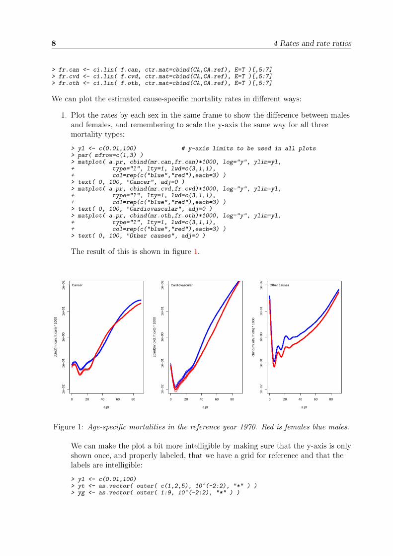
So first we extract the age-specific rates for the reference period defined above. Thecontrast matrices CA and CA.ref are placed beside each other (using cbind(), so theircolumns correspond to all parameters in the model. The argument E=T causes theexponential of the estimates (with c.i.) to be computed and placed in columns 5–7 of theresult, which we then select (see the documentation for ci.lin):

> mr.can <- ci.lin( m.can, ctr.mat=cbind(CA,CA.ref), E=T )[,5:7]> mr.cvd <- ci.lin( m.cvd, ctr.mat=cbind(CA,CA.ref), E=T )[,5:7]> mr.oth <- ci.lin( m.oth, ctr.mat=cbind(CA,CA.ref), E=T )[,5:7]

8 4 Rates and rate-ratios

> fr.can <- ci.lin( f.can, ctr.mat=cbind(CA,CA.ref), E=T )[,5:7]> fr.cvd <- ci.lin( f.cvd, ctr.mat=cbind(CA,CA.ref), E=T )[,5:7]> fr.oth <- ci.lin( f.oth, ctr.mat=cbind(CA,CA.ref), E=T )[,5:7]

We can plot the estimated cause-specific mortality rates in different ways:

1. Plot the rates by each sex in the same frame to show the difference between malesand females, and remembering to scale the y-axis the same way for all threemortality types:

> yl <- c(0.01,100) # y-axis limits to be used in all plots> par( mfrow=c(1,3) )> matplot( a.pr, cbind(mr.can,fr.can)*1000, log="y", ylim=yl,+ type="l", lty=1, lwd=c(3,1,1),+ col=rep(c("blue","red"),each=3) )> text( 0, 100, "Cancer", adj=0 )> matplot( a.pr, cbind(mr.cvd,fr.cvd)*1000, log="y", ylim=yl,+ type="l", lty=1, lwd=c(3,1,1),+ col=rep(c("blue","red"),each=3) )> text( 0, 100, "Cardiovascular", adj=0 )> matplot( a.pr, cbind(mr.oth,fr.oth)*1000, log="y", ylim=yl,+ type="l", lty=1, lwd=c(3,1,1),+ col=rep(c("blue","red"),each=3) )> text( 0, 100, "Other causes", adj=0 )

The result of this is shown in figure 1.

0 20 40 60 80

1e−

021e

−01

1e+

001e

+01

1e+

02

a.pr

cbin

d(m

r.can

, fr.c

an)

* 10

00

Cancer

0 20 40 60 80

1e−

021e

−01

1e+

001e

+01

1e+

02

a.pr

cbin

d(m

r.cvd

, fr.c

vd)

* 10

00

Cardiovascular

0 20 40 60 80

1e−

021e

−01

1e+

001e

+01

1e+

02

a.pr

cbin

d(m

r.oth

, fr.o

th)

* 10

00

Other causes

Figure 1: Age-specific mortalities in the reference year 1970. Red is females blue males.

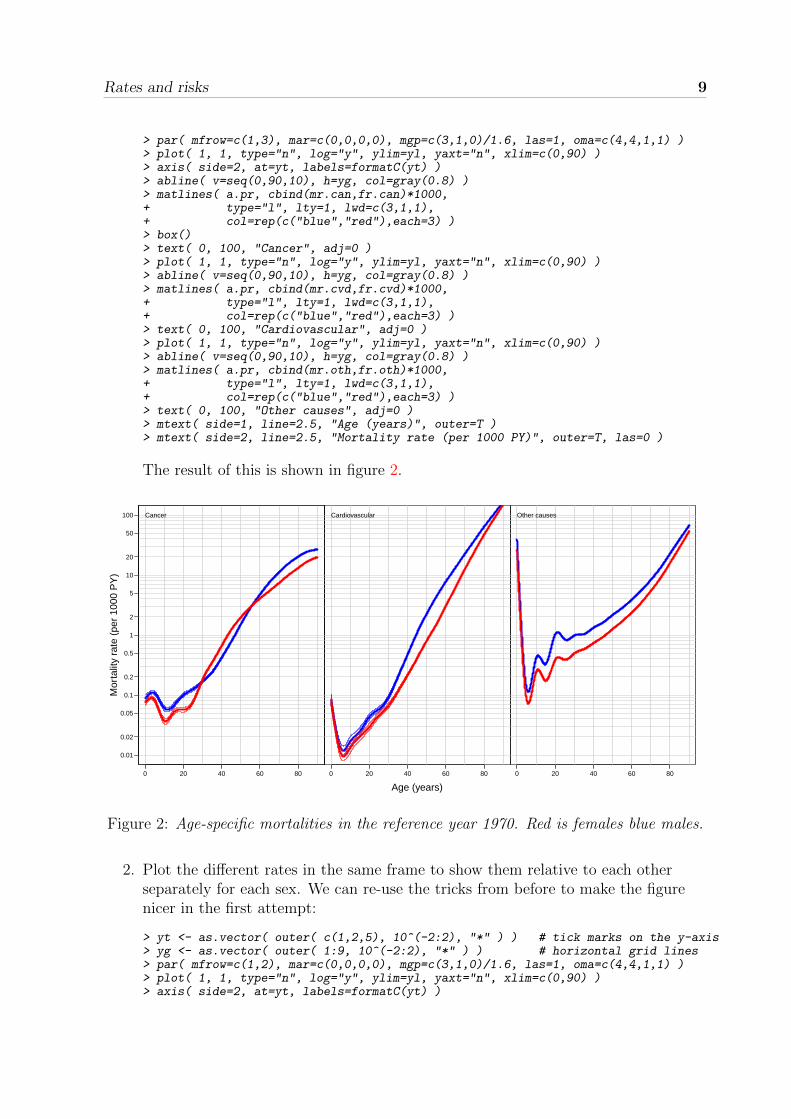
We can make the plot a bit more intelligible by making sure that the y-axis is onlyshown once, and properly labeled, that we have a grid for reference and that thelabels are intelligible:

> yl <- c(0.01,100)> yt <- as.vector( outer( c(1,2,5), 10^(-2:2), "*" ) )> yg <- as.vector( outer( 1:9, 10^(-2:2), "*" ) )

Rates and risks 9

> par( mfrow=c(1,3), mar=c(0,0,0,0), mgp=c(3,1,0)/1.6, las=1, oma=c(4,4,1,1) )> plot( 1, 1, type="n", log="y", ylim=yl, yaxt="n", xlim=c(0,90) )> axis( side=2, at=yt, labels=formatC(yt) )> abline( v=seq(0,90,10), h=yg, col=gray(0.8) )> matlines( a.pr, cbind(mr.can,fr.can)*1000,+ type="l", lty=1, lwd=c(3,1,1),+ col=rep(c("blue","red"),each=3) )> box()> text( 0, 100, "Cancer", adj=0 )> plot( 1, 1, type="n", log="y", ylim=yl, yaxt="n", xlim=c(0,90) )> abline( v=seq(0,90,10), h=yg, col=gray(0.8) )> matlines( a.pr, cbind(mr.cvd,fr.cvd)*1000,+ type="l", lty=1, lwd=c(3,1,1),+ col=rep(c("blue","red"),each=3) )> text( 0, 100, "Cardiovascular", adj=0 )> plot( 1, 1, type="n", log="y", ylim=yl, yaxt="n", xlim=c(0,90) )> abline( v=seq(0,90,10), h=yg, col=gray(0.8) )> matlines( a.pr, cbind(mr.oth,fr.oth)*1000,+ type="l", lty=1, lwd=c(3,1,1),+ col=rep(c("blue","red"),each=3) )> text( 0, 100, "Other causes", adj=0 )> mtext( side=1, line=2.5, "Age (years)", outer=T )> mtext( side=2, line=2.5, "Mortality rate (per 1000 PY)", outer=T, las=0 )


0 20 40 60 80

1

1

0.01

0.02

0.05

0.1

0.2

0.5

1

2

5

10

20

50

100 Cancer

0 20 40 60 80

1

1

Cardiovascular

0 20 40 60 80

1

1

Other causes

Age (years)

Mor

talit

y ra

te (

per

1000

PY

)

Figure 2: Age-specific mortalities in the reference year 1970. Red is females blue males.

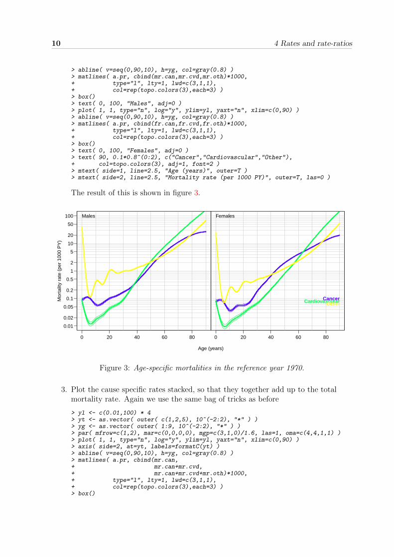
2. Plot the different rates in the same frame to show them relative to each otherseparately for each sex. We can re-use the tricks from before to make the figurenicer in the first attempt:

> yt <- as.vector( outer( c(1,2,5), 10^(-2:2), "*" ) ) # tick marks on the y-axis> yg <- as.vector( outer( 1:9, 10^(-2:2), "*" ) ) # horizontal grid lines> par( mfrow=c(1,2), mar=c(0,0,0,0), mgp=c(3,1,0)/1.6, las=1, oma=c(4,4,1,1) )> plot( 1, 1, type="n", log="y", ylim=yl, yaxt="n", xlim=c(0,90) )> axis( side=2, at=yt, labels=formatC(yt) )

10 4 Rates and rate-ratios

> abline( v=seq(0,90,10), h=yg, col=gray(0.8) )> matlines( a.pr, cbind(mr.can,mr.cvd,mr.oth)*1000,+ type="l", lty=1, lwd=c(3,1,1),+ col=rep(topo.colors(3),each=3) )> box()> text( 0, 100, "Males", adj=0 )> plot( 1, 1, type="n", log="y", ylim=yl, yaxt="n", xlim=c(0,90) )> abline( v=seq(0,90,10), h=yg, col=gray(0.8) )> matlines( a.pr, cbind(fr.can,fr.cvd,fr.oth)*1000,+ type="l", lty=1, lwd=c(3,1,1),+ col=rep(topo.colors(3),each=3) )> box()> text( 0, 100, "Females", adj=0 )> text( 90, 0.1*0.8^(0:2), c("Cancer","Cardiovascular","Other"),+ col=topo.colors(3), adj=1, font=2 )> mtext( side=1, line=2.5, "Age (years)", outer=T )> mtext( side=2, line=2.5, "Mortality rate (per 1000 PY)", outer=T, las=0 )


0 20 40 60 80

1

1

0.01

0.02

0.05

0.1

0.2

0.5

1

2

5

10

20

50

100 Males

0 20 40 60 80

1

1

Females

CancerCardiovascularOther

Age (years)

Mor

talit

y ra

te (

per

1000

PY

)

Figure 3: Age-specific mortalities in the reference year 1970.

3. Plot the cause specific rates stacked, so that they together add up to the totalmortality rate. Again we use the same bag of tricks as before

> yl <- c(0.01,100) * 4> yt <- as.vector( outer( c(1,2,5), 10^(-2:2), "*" ) )> yg <- as.vector( outer( 1:9, 10^(-2:2), "*" ) )> par( mfrow=c(1,2), mar=c(0,0,0,0), mgp=c(3,1,0)/1.6, las=1, oma=c(4,4,1,1) )> plot( 1, 1, type="n", log="y", ylim=yl, yaxt="n", xlim=c(0,90) )> axis( side=2, at=yt, labels=formatC(yt) )> abline( v=seq(0,90,10), h=yg, col=gray(0.8) )> matlines( a.pr, cbind(mr.can,+ mr.can+mr.cvd,+ mr.can+mr.cvd+mr.oth)*1000,+ type="l", lty=1, lwd=c(3,1,1),+ col=rep(topo.colors(3),each=3) )> box()

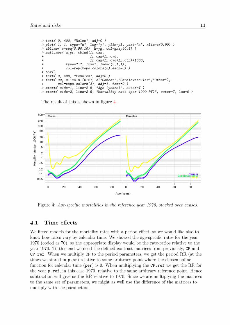
Rates and risks 11

> text( 0, 400, "Males", adj=0 )> plot( 1, 1, type="n", log="y", ylim=yl, yaxt="n", xlim=c(0,90) )> abline( v=seq(0,90,10), h=yg, col=gray(0.8) )> matlines( a.pr, cbind(fr.can,+ fr.can+fr.cvd,+ fr.can+fr.cvd+fr.oth)*1000,+ type="l", lty=1, lwd=c(3,1,1),+ col=rep(topo.colors(3),each=3) )> box()> text( 0, 400, "Females", adj=0 )> text( 90, 0.1*0.8^(0:2), c("Cancer","Cardiovascular","Other"),+ col=topo.colors(3), adj=1, font=2 )> mtext( side=1, line=2.5, "Age (years)", outer=T )> mtext( side=2, line=2.5, "Mortality rate (per 1000 PY)", outer=T, las=0 )


0 20 40 60 80

1

1

0.05

0.1

0.2

0.5

1

2

5

10

20

50

100

200

500 Males

0 20 40 60 80

1

1Females

CancerCardiovascularOther

Age (years)

Mor

talit

y ra

te (

per

1000

PY

)

Figure 4: Age-specific mortalities in the reference year 1970, stacked over causes.

4.1 Time effects

We fitted models for the mortality rates with a period effect, so we would like also toknow how rates vary by calendar time. We showed the age-specific rates for the year1970 (coded as 70), so the appropriate display would be the rate-ratios relative to theyear 1970. To this end we need the defined contrast matrices from previously, CP andCP.ref. When we multiply CP to the period parameters, we get the period RR (at thetimes we stored in p.pr) relative to some arbitrary point where the chosen splinefunction for calendar time (per) is 0. When multiplying the CP.ref we get the RR forthe year p.ref, in this case 1970, relative to the same arbitrary reference point. Hencesubtraction will give us the RR relative to 1970. Since we are multiplying the matricesto the same set of parameters, we might as well use the difference of the matrices tomultiply with the parameters.

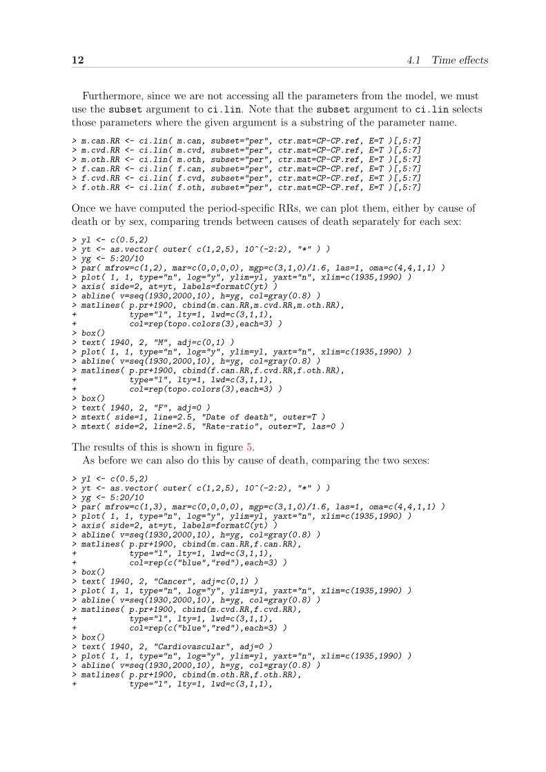
12 4.1 Time effects

Furthermore, since we are not accessing all the parameters from the model, we mustuse the subset argument to ci.lin. Note that the subset argument to ci.lin selectsthose parameters where the given argument is a substring of the parameter name.

> m.can.RR <- ci.lin( m.can, subset="per", ctr.mat=CP-CP.ref, E=T )[,5:7]> m.cvd.RR <- ci.lin( m.cvd, subset="per", ctr.mat=CP-CP.ref, E=T )[,5:7]> m.oth.RR <- ci.lin( m.oth, subset="per", ctr.mat=CP-CP.ref, E=T )[,5:7]> f.can.RR <- ci.lin( f.can, subset="per", ctr.mat=CP-CP.ref, E=T )[,5:7]> f.cvd.RR <- ci.lin( f.cvd, subset="per", ctr.mat=CP-CP.ref, E=T )[,5:7]> f.oth.RR <- ci.lin( f.oth, subset="per", ctr.mat=CP-CP.ref, E=T )[,5:7]

Once we have computed the period-specific RRs, we can plot them, either by cause ofdeath or by sex, comparing trends between causes of death separately for each sex:

> yl <- c(0.5,2)> yt <- as.vector( outer( c(1,2,5), 10^(-2:2), "*" ) )> yg <- 5:20/10> par( mfrow=c(1,2), mar=c(0,0,0,0), mgp=c(3,1,0)/1.6, las=1, oma=c(4,4,1,1) )> plot( 1, 1, type="n", log="y", ylim=yl, yaxt="n", xlim=c(1935,1990) )> axis( side=2, at=yt, labels=formatC(yt) )> abline( v=seq(1930,2000,10), h=yg, col=gray(0.8) )> matlines( p.pr+1900, cbind(m.can.RR,m.cvd.RR,m.oth.RR),+ type="l", lty=1, lwd=c(3,1,1),+ col=rep(topo.colors(3),each=3) )> box()> text( 1940, 2, "M", adj=c(0,1) )> plot( 1, 1, type="n", log="y", ylim=yl, yaxt="n", xlim=c(1935,1990) )> abline( v=seq(1930,2000,10), h=yg, col=gray(0.8) )> matlines( p.pr+1900, cbind(f.can.RR,f.cvd.RR,f.oth.RR),+ type="l", lty=1, lwd=c(3,1,1),+ col=rep(topo.colors(3),each=3) )> box()> text( 1940, 2, "F", adj=0 )> mtext( side=1, line=2.5, "Date of death", outer=T )> mtext( side=2, line=2.5, "Rate-ratio", outer=T, las=0 )

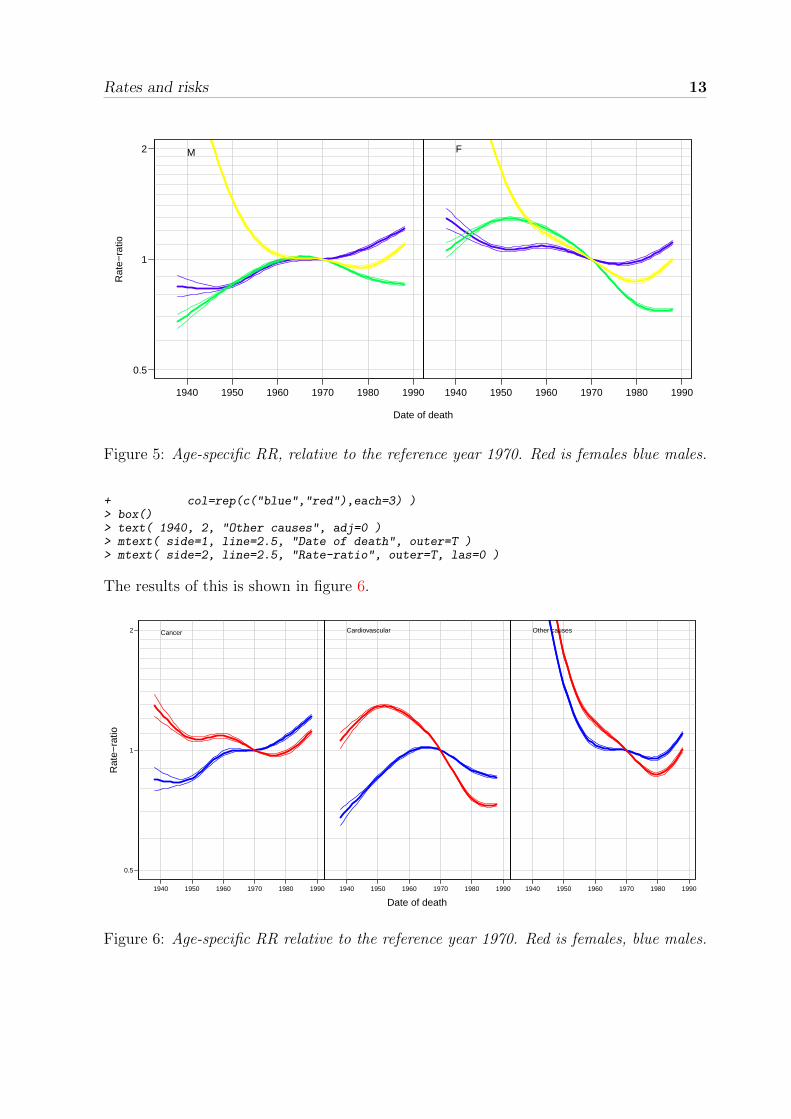
The results of this is shown in figure 5.As before we can also do this by cause of death, comparing the two sexes:

> yl <- c(0.5,2)> yt <- as.vector( outer( c(1,2,5), 10^(-2:2), "*" ) )> yg <- 5:20/10> par( mfrow=c(1,3), mar=c(0,0,0,0), mgp=c(3,1,0)/1.6, las=1, oma=c(4,4,1,1) )> plot( 1, 1, type="n", log="y", ylim=yl, yaxt="n", xlim=c(1935,1990) )> axis( side=2, at=yt, labels=formatC(yt) )> abline( v=seq(1930,2000,10), h=yg, col=gray(0.8) )> matlines( p.pr+1900, cbind(m.can.RR,f.can.RR),+ type="l", lty=1, lwd=c(3,1,1),+ col=rep(c("blue","red"),each=3) )> box()> text( 1940, 2, "Cancer", adj=c(0,1) )> plot( 1, 1, type="n", log="y", ylim=yl, yaxt="n", xlim=c(1935,1990) )> abline( v=seq(1930,2000,10), h=yg, col=gray(0.8) )> matlines( p.pr+1900, cbind(m.cvd.RR,f.cvd.RR),+ type="l", lty=1, lwd=c(3,1,1),+ col=rep(c("blue","red"),each=3) )> box()> text( 1940, 2, "Cardiovascular", adj=0 )> plot( 1, 1, type="n", log="y", ylim=yl, yaxt="n", xlim=c(1935,1990) )> abline( v=seq(1930,2000,10), h=yg, col=gray(0.8) )> matlines( p.pr+1900, cbind(m.oth.RR,f.oth.RR),+ type="l", lty=1, lwd=c(3,1,1),

Rates and risks 13

1940 1950 1960 1970 1980 1990

1

1

0.5

1

2 M

1940 1950 1960 1970 1980 1990

11

F

Date of death

Rat

e−ra

tio

Figure 5: Age-specific RR, relative to the reference year 1970. Red is females blue males.

+ col=rep(c("blue","red"),each=3) )> box()> text( 1940, 2, "Other causes", adj=0 )> mtext( side=1, line=2.5, "Date of death", outer=T )> mtext( side=2, line=2.5, "Rate-ratio", outer=T, las=0 )

The results of this is shown in figure 6.

1940 1950 1960 1970 1980 1990

1

1

0.5

1

2 Cancer

1940 1950 1960 1970 1980 1990

1

1

Cardiovascular

1940 1950 1960 1970 1980 1990

1

1

Other causes

Date of death

Rat

e−ra

tio

Figure 6: Age-specific RR relative to the reference year 1970. Red is females, blue males.

14 4.2 Cumulative risks

4.2 Cumulative risks

The cumulative risks for each cause are the probabilities that a person ends up deadfrom a given cause of death. The formulae for computing these probabilities are in thecase where we have say 3 causes of death, all rely on the survival function, i.e. theprobability of being alive at some time:

S(t) = exp

(−∫ t

0

µcan(u) + µcvd(u) + µoth(u) du

)The probability of being dead from each of the three causes are:

pdead from cancer(t) =

∫ t

0

S(u)µcan(u) du

pdead from CVD(t) =

∫ t

0

S(u)µcvd(u) du

pdead from other causes(t) =

∫ t

0

S(u)µoth(u) du

These formulae are easily transformed into R-code, exploiting that we already havecomputed the mortality rates by age. Note that the age-specific mortality rates(referring to the calendar time 1970) are stored in the variables mr.can, mr.cvd mr.oth

for men and the corresponding variables for women; this was done by the calculationsshown on page 7.

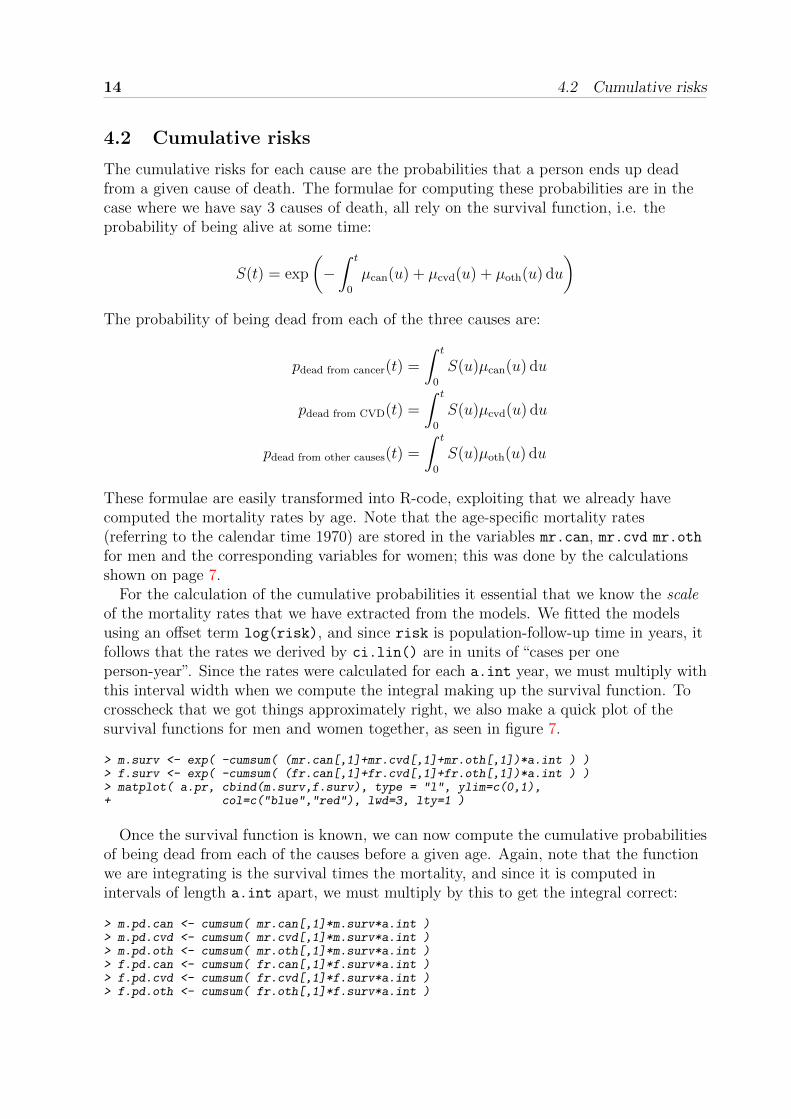
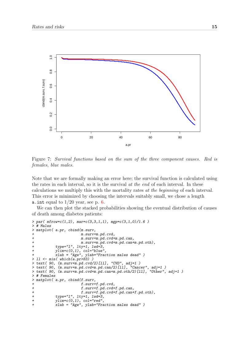
For the calculation of the cumulative probabilities it essential that we know the scaleof the mortality rates that we have extracted from the models. We fitted the modelsusing an offset term log(risk), and since risk is population-follow-up time in years, itfollows that the rates we derived by ci.lin() are in units of “cases per oneperson-year”. Since the rates were calculated for each a.int year, we must multiply withthis interval width when we compute the integral making up the survival function. Tocrosscheck that we got things approximately right, we also make a quick plot of thesurvival functions for men and women together, as seen in figure 7.

> m.surv <- exp( -cumsum( (mr.can[,1]+mr.cvd[,1]+mr.oth[,1])*a.int ) )> f.surv <- exp( -cumsum( (fr.can[,1]+fr.cvd[,1]+fr.oth[,1])*a.int ) )> matplot( a.pr, cbind(m.surv,f.surv), type = "l", ylim=c(0,1),+ col=c("blue","red"), lwd=3, lty=1 )

Once the survival function is known, we can now compute the cumulative probabilitiesof being dead from each of the causes before a given age. Again, note that the functionwe are integrating is the survival times the mortality, and since it is computed inintervals of length a.int apart, we must multiply by this to get the integral correct:

> m.pd.can <- cumsum( mr.can[,1]*m.surv*a.int )> m.pd.cvd <- cumsum( mr.cvd[,1]*m.surv*a.int )> m.pd.oth <- cumsum( mr.oth[,1]*m.surv*a.int )> f.pd.can <- cumsum( fr.can[,1]*f.surv*a.int )> f.pd.cvd <- cumsum( fr.cvd[,1]*f.surv*a.int )> f.pd.oth <- cumsum( fr.oth[,1]*f.surv*a.int )

Rates and risks 15

0 20 40 60 80

0.0

0.2

0.4

0.6

0.8

1.0

a.pr

cbin

d(m

.sur

v, f.

surv

)

Figure 7: Survival functions based on the sum of the three component causes. Red isfemales, blue males.

Note that we are formally making an error here; the survival function is calculated usingthe rates in each interval, so it is the survival at the end of each interval. In thesecalculations we multiply this with the mortality rates at the beginning of each interval.This error is minimized by choosing the intervals suitably small, we chose a lengtha.int equal to 1/20 year, see p. 6.

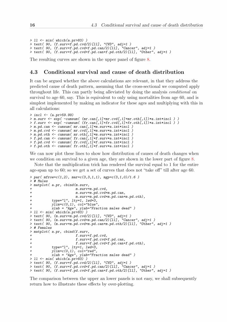
We can then plot the stacked probabilities showing the eventual distribution of causesof death among diabetes patients:

> par( mfrow=c(1,2), mar=c(3,3,1,1), mgp=c(3,1,0)/1.6 )> # Males> matplot( a.pr, cbind(m.surv,+ m.surv+m.pd.cvd,+ m.surv+m.pd.cvd+m.pd.can,+ m.surv+m.pd.cvd+m.pd.can+m.pd.oth),+ type="l", lty=1, lwd=3,+ ylim=c(0,1), col="blue",+ xlab = "Age", ylab="Fraction males dead" )> ll <- min( which(a.pr>83) )> text( 90, (m.surv+m.pd.cvd/2)[ll], "CVD", adj=1 )> text( 90, (m.surv+m.pd.cvd+m.pd.can/2)[ll], "Cancer", adj=1 )> text( 90, (m.surv+m.pd.cvd+m.pd.can+m.pd.oth/2)[ll], "Other", adj=1 )> # Females> matplot( a.pr, cbind(f.surv,+ f.surv+f.pd.cvd,+ f.surv+f.pd.cvd+f.pd.can,+ f.surv+f.pd.cvd+f.pd.can+f.pd.oth),+ type="l", lty=1, lwd=3,+ ylim=c(0,1), col="red",+ xlab = "Age", ylab="Fraction males dead" )

16 4.3 Conditional survival and cause of death distribution

> ll <- min( which(a.pr>83) )> text( 90, (f.surv+f.pd.cvd/2)[ll], "CVD", adj=1 )> text( 90, (f.surv+f.pd.cvd+f.pd.can/2)[ll], "Cancer", adj=1 )> text( 90, (f.surv+f.pd.cvd+f.pd.can+f.pd.oth/2)[ll], "Other", adj=1 )

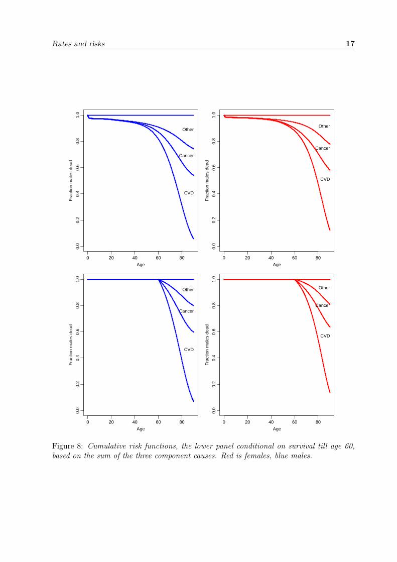
The resulting curves are shown in the upper panel of figure 8.

4.3 Conditional survival and cause of death distribution

It can be argued whether the above calculations are relevant, in that they address thepredicted cause of death pattern, assuming that the cross-sectional we computed applythroughout life. This can partly being alleviated by doing the analysis conditional onsurvival to age 60, say. This is equivalent to only using mortalities from age 60, and issimplest implemented by making an indicator for these ages and multiplying with this inall calculations:

> incl <- (a.pr>59.99)> m.surv <- exp( -cumsum( (mr.can[,1]+mr.cvd[,1]+mr.oth[,1])*a.int*incl ) )> f.surv <- exp( -cumsum( (fr.can[,1]+fr.cvd[,1]+fr.oth[,1])*a.int*incl ) )> m.pd.can <- cumsum( mr.can[,1]*m.surv*a.int*incl )> m.pd.cvd <- cumsum( mr.cvd[,1]*m.surv*a.int*incl )> m.pd.oth <- cumsum( mr.oth[,1]*m.surv*a.int*incl )> f.pd.can <- cumsum( fr.can[,1]*f.surv*a.int*incl )> f.pd.cvd <- cumsum( fr.cvd[,1]*f.surv*a.int*incl )> f.pd.oth <- cumsum( fr.oth[,1]*f.surv*a.int*incl )

We can now plot these lines to show how distribution of causes of death changes whenwe condition on survival to a given age, they are shown in the lower part of figure 8.

Note that the multiplication trick has rendered the survival equal to 1 for the entireage-span up to 60; so we get a set of curves that does not “take off” till after age 60.

> par( mfrow=c(1,2), mar=c(3,3,1,1), mgp=c(3,1,0)/1.6 )> # Males> matplot( a.pr, cbind(m.surv,+ m.surv+m.pd.cvd,+ m.surv+m.pd.cvd+m.pd.can,+ m.surv+m.pd.cvd+m.pd.can+m.pd.oth),+ type="l", lty=1, lwd=3,+ ylim=c(0,1), col="blue",+ xlab = "Age", ylab="Fraction males dead" )> ll <- min( which(a.pr>83) )> text( 90, (m.surv+m.pd.cvd/2)[ll], "CVD", adj=1 )> text( 90, (m.surv+m.pd.cvd+m.pd.can/2)[ll], "Cancer", adj=1 )> text( 90, (m.surv+m.pd.cvd+m.pd.can+m.pd.oth/2)[ll], "Other", adj=1 )> # Females> matplot( a.pr, cbind(f.surv,+ f.surv+f.pd.cvd,+ f.surv+f.pd.cvd+f.pd.can,+ f.surv+f.pd.cvd+f.pd.can+f.pd.oth),+ type="l", lty=1, lwd=3,+ ylim=c(0,1), col="red",+ xlab = "Age", ylab="Fraction males dead" )> ll <- min( which(a.pr>83) )> text( 90, (f.surv+f.pd.cvd/2)[ll], "CVD", adj=1 )> text( 90, (f.surv+f.pd.cvd+f.pd.can/2)[ll], "Cancer", adj=1 )> text( 90, (f.surv+f.pd.cvd+f.pd.can+f.pd.oth/2)[ll], "Other", adj=1 )

The comparison between the upper an lower panels is not easy, we shall subsequentlyreturn how to illustrate these effects by over-plotting.

Rates and risks 17

0 20 40 60 80

0.0

0.2

0.4

0.6

0.8

1.0

Age

Fra

ctio

n m

ales

dea

d

CVD

Cancer

Other

0 20 40 60 80

0.0

0.2

0.4

0.6

0.8

1.0

Age

Fra

ctio

n m

ales

dea

d

CVD

Cancer

Other

0 20 40 60 80

0.0

0.2

0.4

0.6

0.8

1.0

Age

Fra

ctio

n m

ales

dea

d

CVD

Cancer

Other

0 20 40 60 80

0.0

0.2

0.4

0.6

0.8

1.0

Age

Fra

ctio

n m

ales

dea

d

CVD

Cancer

Other

Figure 8: Cumulative risk functions, the lower panel conditional on survival till age 60,based on the sum of the three component causes. Red is females, blue males.

18 5 Tidying the code — some R-tricks exemplified

5 Tidying the code — some R-tricks exemplified

5.1 Setting up an array

In the above section we have done computations separately for men and women and foreach of three causes of death, and we have computed cumulative risks to ages 0–90.Moreover we also conditioned on survival to age 60, but we may want to expand this toa whole sequence of ages of conditioning.

Thus we have three factors across which we want to do the calculations and the plots.It would therefore be convenient if we could just have the relevant code once, and collectthe relevant results in a data structure that allows us to access it later.

The structure which is used for this sort of data collection is an array. It is basically amultidimensional table, where you can refer to the elements by indices.

The input to all our analyses are the mortality rates; the single rates are classified bysex (2 levels), cause (3 levels) and age (90 levels, say). Hence we set up an array withthese dimensions and the fill the rates into it. First the array, which we initialize by NAsand then specify the dimensions

> rates <- array( NA, dim=c(2,3,90) )

We would like to be able to refer to the elements of the array by names in thedimensions, so we would also stick in a dimnames argument, which is a named list:

> rates <- array( NA, dim=c(2,3,90),+ dimnames=list(sex=c("M","F"),+ cause=c("can","cvd","oth"),+ age=0:89) )> dim( rates )

[1] 2 3 90

> dimnames( rates )

$sex[1] "M" "F"

$cause[1] "can" "cvd" "oth"

$age[1] "0" "1" "2" "3" "4" "5" "6" "7" "8" "9" "10" "11" "12" "13" "14"[16] "15" "16" "17" "18" "19" "20" "21" "22" "23" "24" "25" "26" "27" "28" "29"[31] "30" "31" "32" "33" "34" "35" "36" "37" "38" "39" "40" "41" "42" "43" "44"[46] "45" "46" "47" "48" "49" "50" "51" "52" "53" "54" "55" "56" "57" "58" "59"[61] "60" "61" "62" "63" "64" "65" "66" "67" "68" "69" "70" "71" "72" "73" "74"[76] "75" "76" "77" "78" "79" "80" "81" "82" "83" "84" "85" "86" "87" "88" "89"

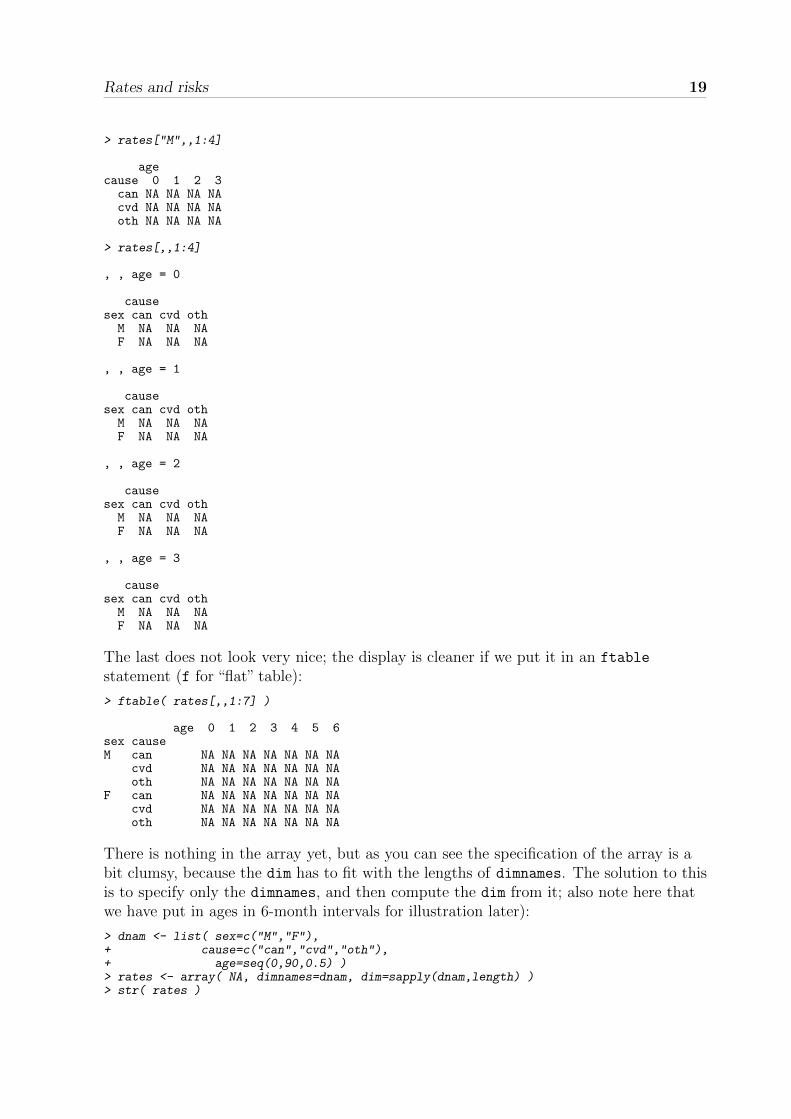
You can now refer to elements of the array either by numbers or names by using a set of“[]”s with three indices, separated by commas. If you leave an empty space betweencommas it is interpreted as all elements along that dimension.

> rates["M",1:2,1:4]

agecause 0 1 2 3can NA NA NA NAcvd NA NA NA NA

Rates and risks 19

> rates["M",,1:4]

agecause 0 1 2 3can NA NA NA NAcvd NA NA NA NAoth NA NA NA NA

> rates[,,1:4]

, , age = 0

causesex can cvd othM NA NA NAF NA NA NA

, , age = 1


, , age = 2


, , age = 3


The last does not look very nice; the display is cleaner if we put it in an ftable

statement (f for “flat” table):

> ftable( rates[,,1:7] )

age 0 1 2 3 4 5 6sex causeM can NA NA NA NA NA NA NA

cvd NA NA NA NA NA NA NAoth NA NA NA NA NA NA NA

F can NA NA NA NA NA NA NAcvd NA NA NA NA NA NA NAoth NA NA NA NA NA NA NA

There is nothing in the array yet, but as you can see the specification of the array is abit clumsy, because the dim has to fit with the lengths of dimnames. The solution to thisis to specify only the dimnames, and then compute the dim from it; also note here thatwe have put in ages in 6-month intervals for illustration later):

> dnam <- list( sex=c("M","F"),+ cause=c("can","cvd","oth"),+ age=seq(0,90,0.5) )> rates <- array( NA, dimnames=dnam, dim=sapply(dnam,length) )> str( rates )

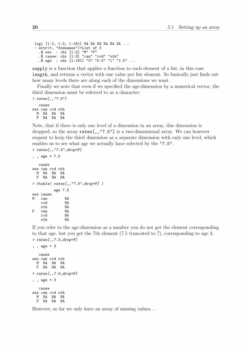
20 5.1 Setting up an array

logi [1:2, 1:3, 1:181] NA NA NA NA NA NA ...- attr(*, "dimnames")=List of 3..$ sex : chr [1:2] "M" "F"..$ cause: chr [1:3] "can" "cvd" "oth"..$ age : chr [1:181] "0" "0.5" "1" "1.5" ...

sapply is a function that applies a function to each element of a list, in this caselength, and returns a vector with one value per list element. So basically just finds outhow many levels there are along each of the dimensions we want.

Finally we note that even if we specified the age-dimension by a numerical vector, thethird dimension must be referred to as a character:> rates[,,"7.5"]


Note, that if there is only one level of a dimension in an array, this dimension isdropped, so the array rates[,,"7.5"] is a two-dimensional array. We can howeverrequest to keep the third dimension as a separate dimension with only one level, whichenables us to see what age we actually have selected by the "7.5":> rates[,,"7.5",drop=F]

, , age = 7.5


> ftable( rates[,,"7.5",drop=F] )

age 7.5sex causeM can NA

cvd NAoth NA

F can NAcvd NAoth NA

If you refer to the age-dimension as a number you do not get the element correspondingto that age, but you get the 7th element (7.5 truncated to 7), corresponding to age 3.> rates[,,7.5,drop=F]

, , age = 3


> rates[,,7.6,drop=F]

, , age = 3


However, so far we only have an array of missing values. . .

Rates and risks 21

5.2 Putting values into the array

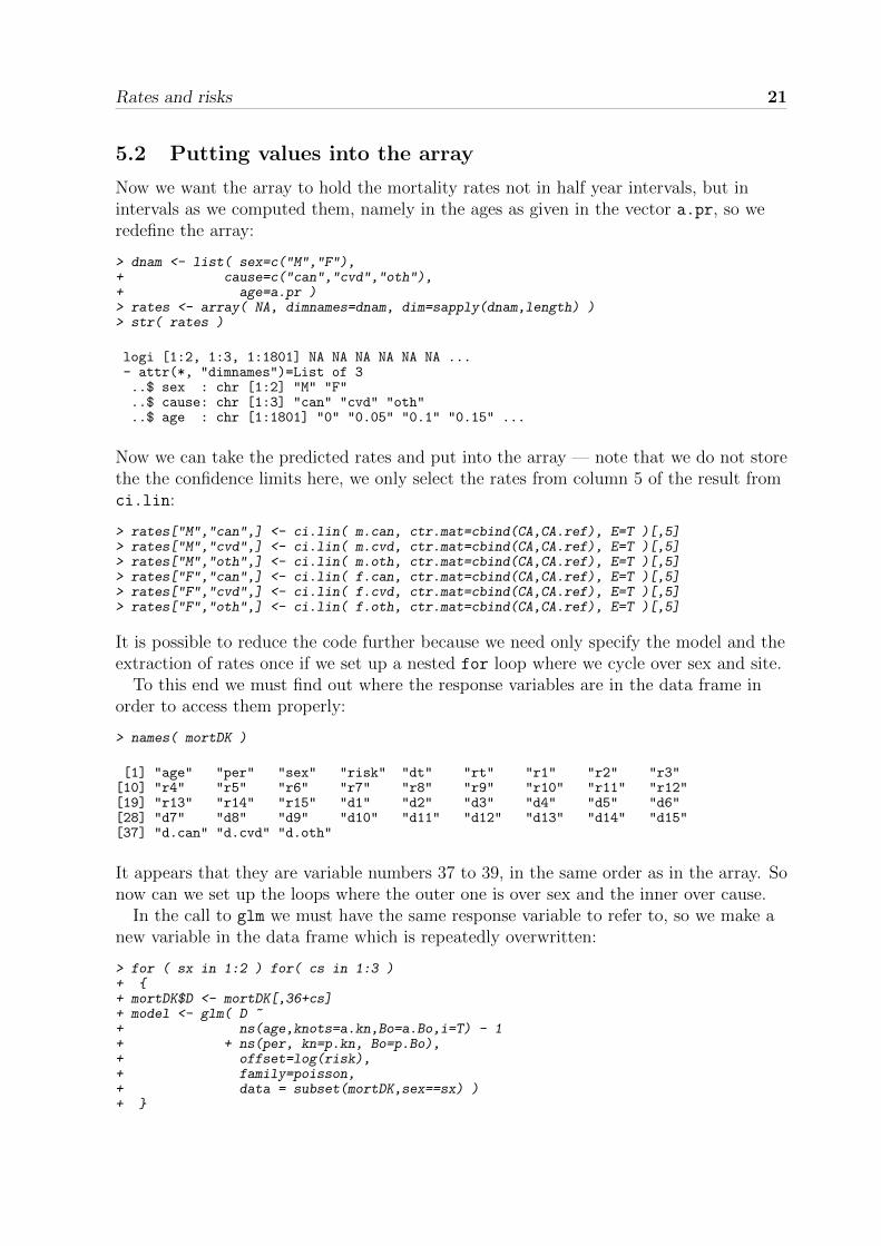
Now we want the array to hold the mortality rates not in half year intervals, but inintervals as we computed them, namely in the ages as given in the vector a.pr, so weredefine the array:

> dnam <- list( sex=c("M","F"),+ cause=c("can","cvd","oth"),+ age=a.pr )> rates <- array( NA, dimnames=dnam, dim=sapply(dnam,length) )> str( rates )

logi [1:2, 1:3, 1:1801] NA NA NA NA NA NA ...- attr(*, "dimnames")=List of 3..$ sex : chr [1:2] "M" "F"..$ cause: chr [1:3] "can" "cvd" "oth"..$ age : chr [1:1801] "0" "0.05" "0.1" "0.15" ...

Now we can take the predicted rates and put into the array — note that we do not storethe the confidence limits here, we only select the rates from column 5 of the result fromci.lin:

> rates["M","can",] <- ci.lin( m.can, ctr.mat=cbind(CA,CA.ref), E=T )[,5]> rates["M","cvd",] <- ci.lin( m.cvd, ctr.mat=cbind(CA,CA.ref), E=T )[,5]> rates["M","oth",] <- ci.lin( m.oth, ctr.mat=cbind(CA,CA.ref), E=T )[,5]> rates["F","can",] <- ci.lin( f.can, ctr.mat=cbind(CA,CA.ref), E=T )[,5]> rates["F","cvd",] <- ci.lin( f.cvd, ctr.mat=cbind(CA,CA.ref), E=T )[,5]> rates["F","oth",] <- ci.lin( f.oth, ctr.mat=cbind(CA,CA.ref), E=T )[,5]

It is possible to reduce the code further because we need only specify the model and theextraction of rates once if we set up a nested for loop where we cycle over sex and site.

To this end we must find out where the response variables are in the data frame inorder to access them properly:

> names( mortDK )

[1] "age" "per" "sex" "risk" "dt" "rt" "r1" "r2" "r3"[10] "r4" "r5" "r6" "r7" "r8" "r9" "r10" "r11" "r12"[19] "r13" "r14" "r15" "d1" "d2" "d3" "d4" "d5" "d6"[28] "d7" "d8" "d9" "d10" "d11" "d12" "d13" "d14" "d15"[37] "d.can" "d.cvd" "d.oth"

It appears that they are variable numbers 37 to 39, in the same order as in the array. Sonow can we set up the loops where the outer one is over sex and the inner over cause.

In the call to glm we must have the same response variable to refer to, so we make anew variable in the data frame which is repeatedly overwritten:

> for ( sx in 1:2 ) for( cs in 1:3 )+ {+ mortDK$D <- mortDK[,36+cs]+ model <- glm( D ~+ ns(age,knots=a.kn,Bo=a.Bo,i=T) - 1+ + ns(per, kn=p.kn, Bo=p.Bo),+ offset=log(risk),+ family=poisson,+ data = subset(mortDK,sex==sx) )+ }

22 5.2 Putting values into the array

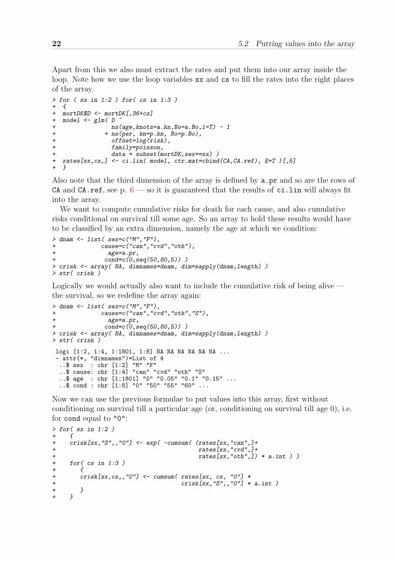
Apart from this we also must extract the rates and put them into our array inside theloop. Note how we use the loop variables sx and cs to fill the rates into the right placesof the array.

> for ( sx in 1:2 ) for( cs in 1:3 )+ {+ mortDK$D <- mortDK[,36+cs]+ model <- glm( D ~+ ns(age,knots=a.kn,Bo=a.Bo,i=T) - 1+ + ns(per, kn=p.kn, Bo=p.Bo),+ offset=log(risk),+ family=poisson,+ data = subset(mortDK,sex==sx) )+ rates[sx,cs,] <- ci.lin( model, ctr.mat=cbind(CA,CA.ref), E=T )[,5]+ }

Also note that the third dimension of the array is defined by a.pr and so are the rows ofCA and CA.ref, see p. 6 — so it is guaranteed that the results of ci.lin will always fitinto the array.

We want to compute cumulative risks for death for each cause, and also cumulativerisks conditional on survival till some age. So an array to hold these results would haveto be classified by an extra dimension, namely the age at which we condition:

> dnam <- list( sex=c("M","F"),+ cause=c("can","cvd","oth"),+ age=a.pr,+ cond=c(0,seq(50,80,5)) )> crisk <- array( NA, dimnames=dnam, dim=sapply(dnam,length) )> str( crisk )

Logically we would actually also want to include the cumulative risk of being alive —the survival, so we redefine the array again:

> dnam <- list( sex=c("M","F"),+ cause=c("can","cvd","oth","S"),+ age=a.pr,+ cond=c(0,seq(50,80,5)) )> crisk <- array( NA, dimnames=dnam, dim=sapply(dnam,length) )> str( crisk )

logi [1:2, 1:4, 1:1801, 1:8] NA NA NA NA NA NA ...- attr(*, "dimnames")=List of 4..$ sex : chr [1:2] "M" "F"..$ cause: chr [1:4] "can" "cvd" "oth" "S"..$ age : chr [1:1801] "0" "0.05" "0.1" "0.15" .....$ cond : chr [1:8] "0" "50" "55" "60" ...

Now we can use the previous formulae to put values into this array, first withoutconditioning on survival till a particular age (or, conditioning on survival till age 0), i.e.for cond equal to "0":

> for( sx in 1:2 )+ {+ crisk[sx,"S",,"0"] <- exp( -cumsum( (rates[sx,"can",]++ rates[sx,"cvd",]++ rates[sx,"oth",]) * a.int ) )+ for( cs in 1:3 )+ {+ crisk[sx,cs,,"0"] <- cumsum( rates[sx, cs, "0"] *+ crisk[sx,"S",,"0"] * a.int )+ }+ }

Rates and risks 23

When we want to condition on survival to a given age we devised a variable which wasthe indicator of age above the age at which we conditioned. So effectively we need a looparound the two we already have that devises this for us. But recall the dimensions of thearrays are characters, so we need to fish out the numeric and then devise the indicator:

Note the following:

> dimnames(crisk)[4]

$cond[1] "0" "50" "55" "60" "65" "70" "75" "80"

> dimnames(crisk)[[4]]

[1] "0" "50" "55" "60" "65" "70" "75" "80"

> as.numeric( dimnames(crisk)[[4]] )

[1] 0 50 55 60 65 70 75 80

The first gives a list with one element, namely the vector of names, technically this is asublist of length 1. The second with the “[[]]” gives the fourth element of the list, inthis case the character vector. But we need the numbers, so it is the last type ofexpression we need in our loop. Actually we also use the character vector as ourloop-variable. Note that this will also work for age 0, and that we subtract a smallamount from the age at which we condition, in order to avoid larger or equal to, sinceequality is alway uncertain on a computer:

> for( ac in dimnames(crisk)[[4]] )+ {+ incl <- ( a.pr > (as.numeric(ac)-a.int/10) )+ for( sx in 1:2 )+ {+ crisk[sx,"S",,ac] <- exp( -cumsum( (rates[sx,"can",]++ rates[sx,"cvd",]++ rates[sx,"oth",]) * a.int * incl ) )+ for( cs in dimnames(rates)[[2]] )+ {+ crisk[sx,cs,,ac] <- cumsum( rates[sx,cs,] *+ crisk[sx,"S",,ac] * a.int * incl )+ }+ }+ }

For further generality, to make the code independent of the number of causes, we notethat the terms rates[sx,"can",] etc. should be replaced by a sum over the first of thetwo dimensions of rates[sx,,] — when the level of the first dimension is fixed theresult is a two-dimensional array. For this purpose we use the function apply, whichapplies a specified function across one or more dimensions of an array. The expressions

> rates[sx,"can",] + rates[sx,"cvd",] + rates[sx,"oth",]

is equivalent to:

> apply( rates[sx,,], 2, sum )

24 5.3 Saving results

which is to interpreted as “apply the function sum on the two-dimensional arrayrates[sx,,] (classified by (cause,age), since we have fixed sex to the current value ofsx), such that the result is classified by dimension 2 of the array (in this case age). Thusthe second argument to apply is the dimension(s) of the original array that will beclassifying the result; the function (in this case sum) is applied to all elements of thearray in each slice along this dimension.

Thus the final generality which also caters for any number of competing risks:

> for( ac in dimnames(crisk)[[4]] )+ {+ incl <- ( a.pr > (as.numeric(ac)-a.int/10) )+ for( sx in dimnames(rates)[[1]] )+ {+ crisk[sx,"S",,ac] <- exp( -cumsum( apply(rates[sx,,],2,sum) * a.int * incl ) )+ for( cs in dimnames(rates)[[2]] )+ {+ crisk[sx,cs,,ac] <- cumsum( rates[sx,cs,] *+ crisk[sx,"S",,ac] * a.int * incl )+ }+ }+ }

So now we have all the modelling and the computation of the rates embedded in twonested loops, that all live off a few variables we have defined up front, such as the causesof death (and where they are stored in the database), the ages at which we condition onsurvival etc.

If we for example had a dataset with two groups of persons, such as diabetes patientsand non-diabetic we would expand the arrays with a DM / non-DM dimension and putan extra loop around the two loops we already have.

The advantage of this approach is that we are absolutely sure that both sexes and allcauses of death are dealt with in the same way, and we have only one place in the codewhere the formulae are translated into code. Moreover, if we for example want to changethe set of ages where we condition on survival to.

5.3 Saving results

Apart from the clarity in the expression of statistical and demographic theory incomputer code, a main reason to collect results in an array is that subsequent plottingand reporting of results in tabular form gets easier. This is particularly the case whenmodel fitting (unlike in this example) takes a long time.

Plotting results is (even in R!) is a trial and error process and therefore it is handy tohave the numbers you actually want to plot collected in an array. Hence you wouldtypically want to save the resulting array(s) for future retrieval:

> save( rates, crisk, file="../data/rates-risk.Rdata" )> load( file="../data/rates-risk.Rdata" )

5.4 Plotting results

When we want make plots of the cumulative probabilities we would do this the sameway we did with the previous plots, but now exploiting the fact that we have have allthe results we want to plot available in an array.

Rates and risks 25

In order to compare males and females we plot the figure for females mirrored, so thefirst try

> matplot( a.pr,+ cbind( crisk["M","S",,"0"],+ crisk["M","S",,"0"]+crisk["M","can",,"0"],+ crisk["M","S",,"0"]+crisk["M","can",,"0"]+crisk["M","cvd",,"0"],+ crisk["M","S",,"0"]+crisk["M","can",,"0"]+crisk["M","cvd",,"0"],+crisk["M","oth",,"0"] ),+ type="l", lty=1, lwd=2, col="blue" )

However, instead we would rather make automatic the cumulative sum over survival andthe causes. This can be done using apply with the function cumsum. The structure ofthe result can be shown this way:

> str( apply(crisk,c(1,3,4),cumsum) )

num [1:4, 1:2, 1:1801, 1:8] 4.34e-06 8.57e-06 1.93e-03 1.00 3.82e-06 ...- attr(*, "dimnames")=List of 4..$ : chr [1:4] "can" "cvd" "oth" "S"..$ sex : chr [1:2] "M" "F"..$ age : chr [1:1801] "0" "0.05" "0.1" "0.15" .....$ cond: chr [1:8] "0" "50" "55" "60" ...

This use of apply has taken cumulative sum along the dimension number 2 for eachslice of the array classified by a combination of the 1st, 3rd and 4th dimension. Theresult is classified by first the dimension returned by cumsum, that is the formerdimension number 2, and then the remaining dimensions (1,3,4).

Moreover the sum is in the order (can, cvd, oth, S), but we would really prefer theorder (S,can, cvd, oth), but this can be fixed by permuting the 2nd dimension beforeusing the apply function:

> str( apply(crisk[,c(4,1,2,3),,],c(1,3,4),cumsum) )

num [1:4, 1:2, 1:1801, 1:8] 0.998 0.998 0.998 1 0.999 ...- attr(*, "dimnames")=List of 4..$ : chr [1:4] "S" "can" "cvd" "oth"..$ sex : chr [1:2] "M" "F"..$ age : chr [1:1801] "0" "0.05" "0.1" "0.15" .....$ cond: chr [1:8] "0" "50" "55" "60" ...

So no we can produce an array of the stacked cumulative risks that we want to plot

> stcr <- apply( crisk[,c(4,1,2,3),,], c(1,3,4), cumsum )> str( stcr )

num [1:4, 1:2, 1:1801, 1:8] 0.998 0.998 0.998 1 0.999 ...- attr(*, "dimnames")=List of 4..$ : chr [1:4] "S" "can" "cvd" "oth"..$ sex : chr [1:2] "M" "F"..$ age : chr [1:1801] "0" "0.05" "0.1" "0.15" .....$ cond: chr [1:8] "0" "50" "55" "60" ...

This enables us to compare males and females directly, by reverting the x-axis of thefemales:

26 5.4 Plotting results

> par( mfrow=c(1,2), mar=c(0,0,0,0), oma=c(3,3,1,3), mgp=c(3,1,0)/1.6,+ las=1, bty="n" )> matplot( a.pr, t(stcr[,"M",,"0"]),+ ylim=c(0,1), xlim=c(0,90), xaxs="i", yaxs="i",+ type="l", lty=1, lwd=3, col="blue", bty="l" )> matplot( a.pr, t(stcr[,"F",,"0"]),+ ylim=c(0,1), xlim=c(90,0), xaxs="i", yaxs="i", yaxt="n",+ type="l", lty=1, lwd=3, col="red", bty="]" )> axis( side=4 )

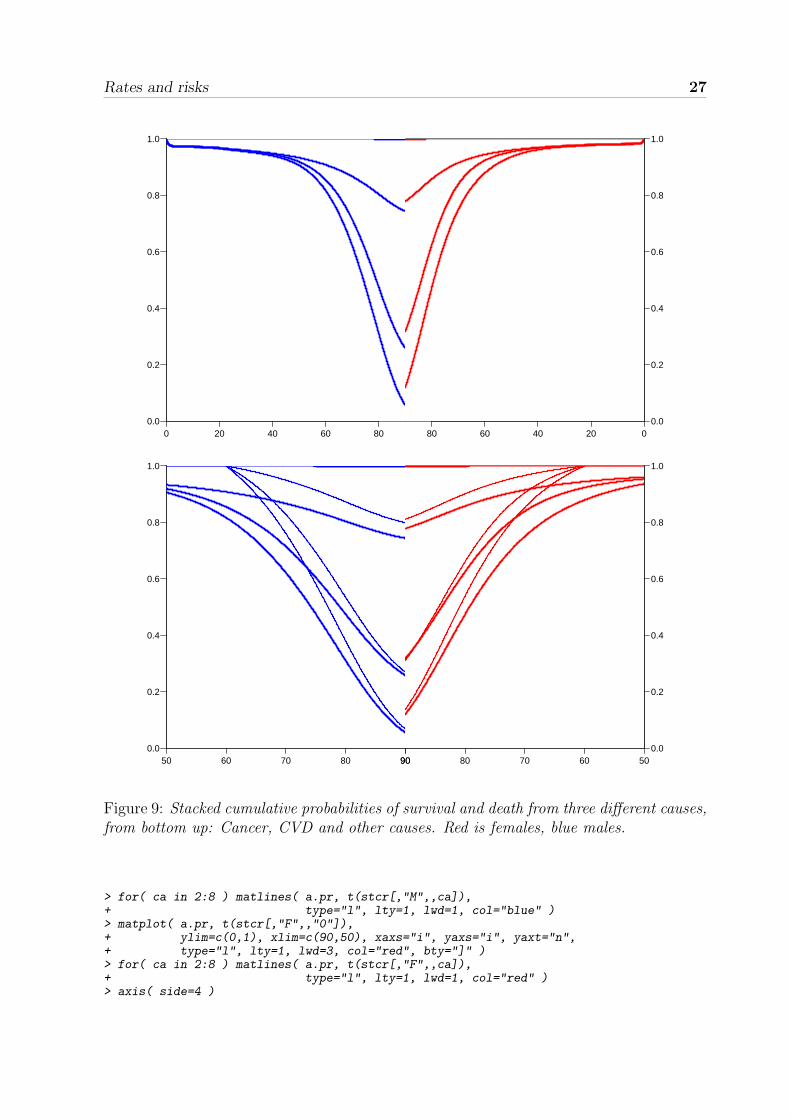
We would also like to plot the conditional probabilities, conditioning on survival till age60. This just requires a matlines extra for each sex, using dotted lines instead todistinguish from the original ones. For clarity we have stretched the age-axis bydiscarding ages under 50:

> par( mfrow=c(1,2), mar=c(0,0,0,0), oma=c(3,3,1,3), mgp=c(3,1,0)/1.6,+ las=1, bty="n" )> matplot( a.pr, t(stcr[,"M",,"0"]),+ ylim=c(0,1), xlim=c(50,90), xaxs="i", yaxs="i",+ type="l", lty=1, lwd=3, col="blue", bty="l" )> matlines( a.pr, t(stcr[,"M",,"60"]),+ type="l", lty=1, lwd=2, col="blue" )> matplot( a.pr, t(stcr[,"F",,"0"]),+ ylim=c(0,1), xlim=c(90,50), xaxs="i", yaxs="i", yaxt="n",+ type="l", lty=1, lwd=3, col="red", bty="]" )> matlines( a.pr, t(stcr[,"F",,"60"]),+ type="l", lty=1, lwd=2, col="red" )> axis( side=4 )

These two plots are shown in figure 9If we want to plot the conditional survivals for all the ages we conditioned on in the

analysis we can simplify things using a for-loop:

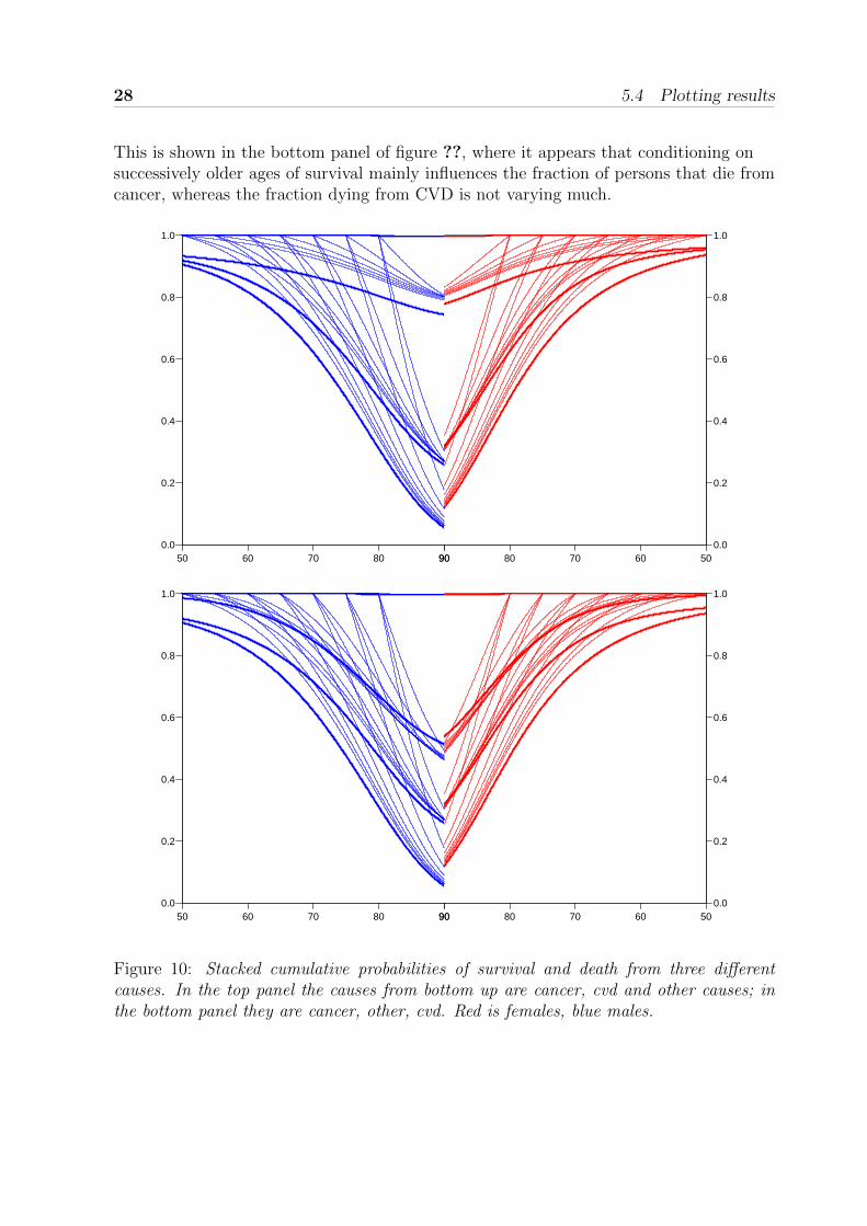
> par( mfrow=c(1,2), mar=c(0,0,0,0), oma=c(3,3,1,3), mgp=c(3,1,0)/1.6,+ las=1, bty="n" )> matplot( a.pr, t(stcr[,"M",,"0"]),+ ylim=c(0,1), xlim=c(50,90), xaxs="i", yaxs="i",+ type="l", lty=1, lwd=3, col="blue", bty="l" )> for( ca in 2:8 ) matlines( a.pr, t(stcr[,"M",,ca]),+ type="l", lty=1, lwd=1, col="blue" )> matplot( a.pr, t(stcr[,"F",,"0"]),+ ylim=c(0,1), xlim=c(90,50), xaxs="i", yaxs="i", yaxt="n",+ type="l", lty=1, lwd=3, col="red", bty="]" )> for( ca in 2:8 ) matlines( a.pr, t(stcr[,"F",,ca]),+ type="l", lty=1, lwd=1, col="red" )> axis( side=4 )

This is shown in the top panel of figure 10.It may be of interest to see this pattern for a different ordering of the causes of death,

for example by interchanging cvd and other causes. This can be very simply achieved bychanging the cumulative summing order when forming stcr, so it is just replacingc(4,1,2,3) by c(4,1,3,2):

> stcr <- apply( crisk[,c(4,1,3,2),,], c(1,3,4), cumsum )> par( mfrow=c(1,2), mar=c(0,0,0,0), oma=c(3,3,1,3), mgp=c(3,1,0)/1.6,+ las=1, bty="n" )> matplot( a.pr, t(stcr[,"M",,"0"]),+ ylim=c(0,1), xlim=c(50,90), xaxs="i", yaxs="i",+ type="l", lty=1, lwd=3, col="blue", bty="l" )

Rates and risks 27

0 20 40 60 800.0

0.2

0.4

0.6

0.8

1.0

a.pr

t(st

cr[,

"M",

, "0

"])

80 60 40 20 0

a.pr

t(st

cr[,

"F",

, "0

"])

0.0

0.2

0.4

0.6

0.8

1.0

50 60 70 80 900.0

0.2

0.4

0.6

0.8

1.0

a.pr

t(st

cr[,

"M",

, "0

"])

90 80 70 60 50

a.pr

t(st

cr[,

"F",

, "0

"])

0.0

0.2

0.4

0.6

0.8

1.0

Figure 9: Stacked cumulative probabilities of survival and death from three different causes,from bottom up: Cancer, CVD and other causes. Red is females, blue males.

> for( ca in 2:8 ) matlines( a.pr, t(stcr[,"M",,ca]),+ type="l", lty=1, lwd=1, col="blue" )> matplot( a.pr, t(stcr[,"F",,"0"]),+ ylim=c(0,1), xlim=c(90,50), xaxs="i", yaxs="i", yaxt="n",+ type="l", lty=1, lwd=3, col="red", bty="]" )> for( ca in 2:8 ) matlines( a.pr, t(stcr[,"F",,ca]),+ type="l", lty=1, lwd=1, col="red" )> axis( side=4 )

28 5.4 Plotting results

This is shown in the bottom panel of figure ??, where it appears that conditioning onsuccessively older ages of survival mainly influences the fraction of persons that die fromcancer, whereas the fraction dying from CVD is not varying much.

50 60 70 80 900.0

0.2

0.4

0.6

0.8

1.0

a.pr

t(st

cr[,

"M",

, "0

"])

90 80 70 60 50

a.pr

t(st

cr[,

"F",

, "0

"])

0.0

0.2

0.4

0.6

0.8

1.0

50 60 70 80 900.0

0.2

0.4

0.6

0.8

1.0

a.pr

t(st

cr[,

"M",

, "0

"])

90 80 70 60 50

a.pr

t(st

cr[,

"F",

, "0

"])

0.0

0.2

0.4

0.6

0.8

1.0

Figure 10: Stacked cumulative probabilities of survival and death from three differentcauses. In the top panel the causes from bottom up are cancer, cvd and other causes; inthe bottom panel they are cancer, other, cvd. Red is females, blue males.

Documents

Rates and (competing) risks: Example calculations using