stcrmix

stcrmix and Timing of Events with Stata

Christophe Kolodziejczyk, VIVE

August 30, 2017

stcrmix

Introduction

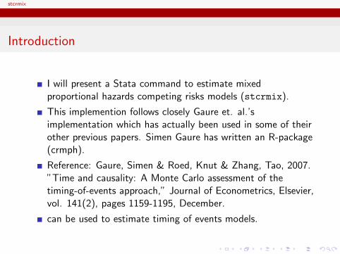
I will present a Stata command to estimate mixedproportional hazards competing risks models (stcrmix).

This implemention follows closely Gaure et. al.’simplementation which has actually been used in some of theirother previous papers. Simen Gaure has written an R-package(crmph).

Reference: Gaure, Simen & Roed, Knut & Zhang, Tao, 2007.”Time and causality: A Monte Carlo assessment of thetiming-of-events approach,” Journal of Econometrics, Elsevier,vol. 141(2), pages 1159-1195, December.

can be used to estimate timing of events models.

stcrmix

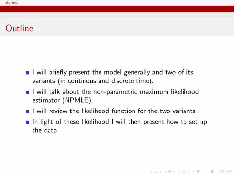
Outline

I will briefly present the model generally and two of itsvariants (in continous and discrete time).

I will talk about the non-parametric maximum likelihoodestimator (NPMLE).

I will review the likelihood function for the two variants

In light of these likelihood I will then present how to set upthe data

stcrmix

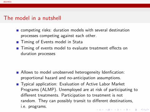
The model in a nutshell

competing risks: duration models with several destinationprocesses competing against each other.

Timing of Events model in Stata

Timing of events model to evaluate treatment effects onduration processes

Treatment effects are also modelled as duration process

Competing risk model

Allows to model unobserved heterogeneity Idenfication:proportional hazard and no-anticipation assumptions.

Typical application: Evaluation of Active Labor MarketPrograms (ALMP). Unemployed are at risk of participating todifferent treatments. Participation to treatment is notrandom. They can possibly transit to different destinations,i.e. programs.

stcrmix

The model in a nutshell

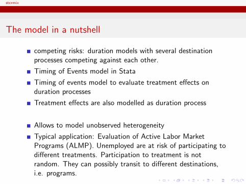
competing risks: duration models with several destinationprocesses competing against each other.

Timing of Events model in Stata

Timing of events model to evaluate treatment effects onduration processes

Treatment effects are also modelled as duration process

Competing risk model

Allows to model unobserved heterogeneity

Typical application: Evaluation of Active Labor MarketPrograms (ALMP). Unemployed are at risk of participating todifferent treatments. Participation to treatment is notrandom. They can possibly transit to different destinations,i.e. programs.

stcrmix

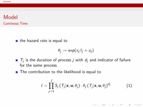
ModelContinous Time

the hazard rate is equal to

θj := exp(xjβj + uj)

Tj is the duration of process j with dj and indicator of failurefor the same process.

The contribution to the likelihood is equal to

` =J∏

j=1

Sj (Tj |x,u; θj) · θj (Tj |x,u; θj)dj (1)

stcrmix

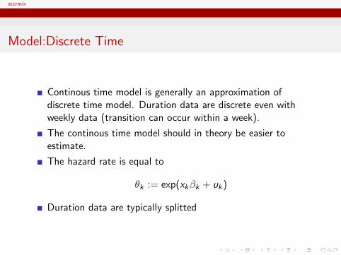
Model:Discrete Time

Continous time model is generally an approximation ofdiscrete time model. Duration data are discrete even withweekly data (transition can occur within a week).

The continous time model should in theory be easier toestimate.

The hazard rate is equal to

θk := exp(xkβk + uk)

Duration data are typically splitted

stcrmix

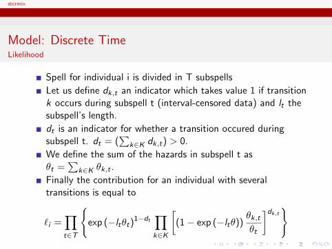
Model: Discrete TimeLikelihood

Spell for individual i is divided in T subspells

Let us define dk,t an indicator which takes value 1 if transitionk occurs during subspell t (interval-censored data) and lt thesubspell’s length.

dt is an indicator for whether a transition occured duringsubspell t. dt = (

∑k∈K dk,t) > 0.

We define the sum of the hazards in subspell t asθt =

∑k∈K θk,t .

Finally the contribution for an individual with severaltransitions is equal to

`i =∏t∈T

{exp (−ltθt)1−dt

∏k∈K

[(1− exp (−ltθ))

θk,tθt

]dk,t}

stcrmix

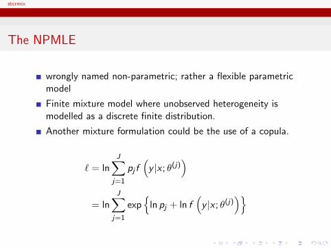
The NPMLE

wrongly named non-parametric; rather a flexible parametricmodel

Finite mixture model where unobserved heterogeneity ismodelled as a discrete finite distribution.

Another mixture formulation could be the use of a copula.

` = lnJ∑

j=1

pj f(y |x ; θ(j)

)

= lnJ∑

j=1

exp{

ln pj + ln f(y |x ; θ(j)

)}

stcrmix

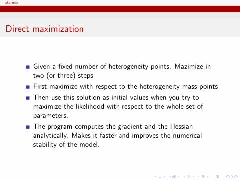
Direct maximization

Given a fixed number of heterogeneity points. Mazimize intwo-(or three) steps

First maximize with respect to the heterogeneity mass-points

Then use this solution as initial values when you try tomaximize the likelihood with respect to the whole set ofparameters.

The program computes the gradient and the Hessiananalytically. Makes it faster and improves the numericalstability of the model.

stcrmix

Direct maximization: choice of algorithm

Combination of BFGS and Newton-Raphson

Switching between algorithms can be effective (but notalways) in getting out of a situation where the optimizer getsstuck.

Stata’s version of Newton-Raphson (NR) is quite effective,but it requires to compute the Hessian which can be costlydepending on the scale of the problem.

BFGS is less costly since in computes an approximation of theHessian based on the gradient, but it is slower in finding asolution, i.e. you need more iteration. But still it can be fasterin finding the solution.

You may use the BHHH/Fisher scoring instead of NR (basedon gradient hence less costly). BHHH uses the outer-productof the gradient. To be combined with BFGS.

stcrmix

Finding new heterogeneity mass-points

Find mass-points which will likely give an improvement in thelikelihood

Simulated Annealing to find a positive Gateaux derivative.

LL[θ1; (p(1− ρ), ρ)

]− LL(θ0; p)

ρ> 0

Simulated annealing: derivative free method to find globaloptimum of a function or at least a reasonably close solutionat a non-prohibitive cost. Slow but robust (or robust butslow).

Heckman and Singer (1984) in the single transition caseproposed to find a m.p. which maximizes the Gateauxderivative. Use grid search. Gaure et al. adivse against it.

stcrmix

When is it finished?

Repeat the process of finding heterogeneity mass-points untilno further improvement in the likelihood.

Add heterogeneity points one at a time. Otherwise you endup with numerical problems.

A popular formulation is to estimate n points for eachtransition and estimate the probability of each combination ofm.p. It is fine with 2 heterogeneity points (still challengingthough...), but with 3 heterogeneity points and 2 transitionsyou have to estimate 8 probabilities.

stcrmix

Estimation problems and possible solutions

Large (negative) values for the mass-points. Solution: treatthese parameters as constants during maximization.

Defect (very small) hazards. Problem occurs when number ofpoints becomes large (7). Risk set is set to zero for theseobservations.

Small probabilities of the heterogeneity mass-points(≤ 0.000001 f.e.). Solution: average these points with thenext adjacent point.

stcrmix

Estimation problems and possible solutions

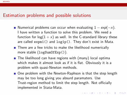
Numerical problems can occur when evaluating 1− exp(−x).I have written a function to solve this problem. We need afunction for log(1 + x) as well. In the C-standard library theseare called expm1() and log1p(). They don’t exist in Mata.

There are a few tricks to make the likelihood numericallymore stable (logSumOfExp()).

The likelihood can have regions with (many) local optimawhich makes it almost look as if it is flat. Obviously it is aproblem with quasi-Newton methods.

One problem with the Newton-Raphson is that the step lengthmay be too long giving you absurd paramaters. UseTrust-region method to limit the step length. Not officiallyimplemented in Stata-Mata.

stcrmix

What can we do with the command (in theory)

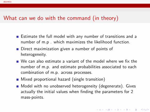
Estimate the full model with any number of transitions and anumber of m.p . which maximizes the likelihood function.

Direct maximization given a number of points ofheterogeneity.

We can also estimate a variant of the model where we fix thenumber of m.p. and estimate probabilities associated to eachcombination of m.p. across processes.

Mixed proportional hazard (single transition)

Model with no unobserved heterogeneity (degenerate). Givesactually the initial values when finding the parameters for 2mass-points.

stcrmix

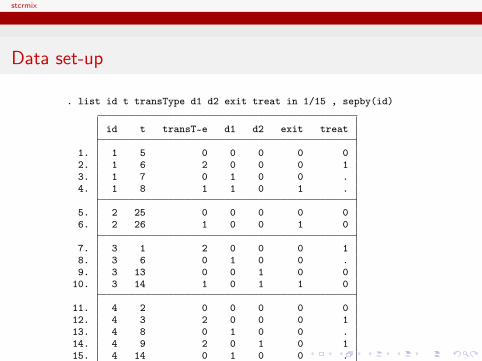
Data set-up

. list id t transType d1 d2 exit treat in 1/15 , sepby(id)

id t transT~e d1 d2 exit treat

1. 1 5 0 0 0 0 02. 1 6 2 0 0 0 13. 1 7 0 1 0 0 .4. 1 8 1 1 0 1 .

5. 2 25 0 0 0 0 06. 2 26 1 0 0 1 0

7. 3 1 2 0 0 0 18. 3 6 0 1 0 0 .9. 3 13 0 0 1 0 0

10. 3 14 1 0 1 1 0

11. 4 2 0 0 0 0 012. 4 3 2 0 0 0 113. 4 8 0 1 0 0 .14. 4 9 2 0 1 0 115. 4 14 0 1 0 0 .

stcrmix

The syntax of the command I

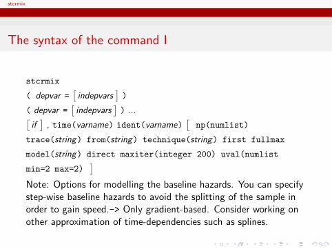
stcrmix

( depvar =[indepvars

])

( depvar =[indepvars

]) ...[

if], time(varname) ident(varname)

[np(numlist)

trace(string) from(string) technique(string) first fullmax

model(string) direct maxiter(integer 200) uval(numlist

min=2 max=2)]

Note: Options for modelling the baseline hazards. You can specifystep-wise baseline hazards to avoid the splitting of the sample inorder to gain speed.-> Only gradient-based. Consider working onother approximation of time-dependencies such as splines.

stcrmix

The syntax of the command II

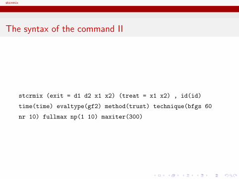
stcrmix (exit = d1 d2 x1 x2) (treat = x1 x2) , id(id)

time(time) evaltype(gf2) method(trust) technique(bfgs 60

nr 10) fullmax np(1 10) maxiter(300)

stcrmix

Simulated data

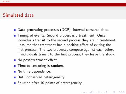
Data generating processes (DGP): interval censored data.

Timing-of-events. Second process is a treatment. Onceindividuals transit to the second process they are in treatment.I assume that treatment has a positive effect of exiting thefirst process. The two processes compete against each other.If individuals transit to the first process, they leave the study.

No post-treatment effect.

Time to censoring is random.

No time dependence.

But unobserved heterogeneity

Solution after 10 points of heterogeneity.

stcrmix

Simulations

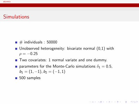
# individuals : 50000

Unobserved heterogeneity: bivariate normal (0,1) withρ = −0.25

Two covariates: 1 normal variate and one dummy.

parameters for the Monte-Carlo simulations δ1 = 0.5,b1 = (1,−1), b2 = (−1, 1)

500 samples

stcrmix

Some results: average og estimated paramaters

Average s.e. low high

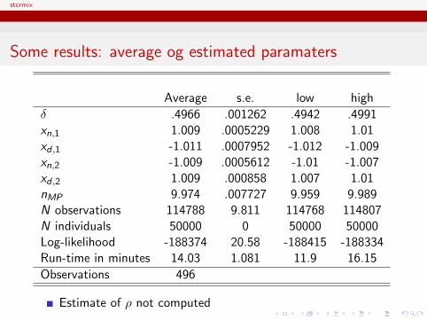
δ .4966 .001262 .4942 .4991xn,1 1.009 .0005229 1.008 1.01xd ,1 -1.011 .0007952 -1.012 -1.009xn,2 -1.009 .0005612 -1.01 -1.007xd ,2 1.009 .000858 1.007 1.01nMP 9.974 .007727 9.959 9.989N observations 114788 9.811 114768 114807N individuals 50000 0 50000 50000Log-likelihood -188374 20.58 -188415 -188334Run-time in minutes 14.03 1.081 11.9 16.15

Observations 496

Estimate of ρ not computed

stcrmix

Some results: distribution of the estimates treatment effect

stcrmix

Further work

Some work needed for the simulations to get results fromNPMLE which takes less time.

the number of covariates is an issue since it makes the modelslower to estimate and thereby limit the number of processesyou can estimate.

In the context of ALMP we would like to evaluate manydifferent employment programs.

Some work necessary on how to compute the likelihood,notably the issue of defect risks.

stcrmix

Summary

I have presented stcrmix: a Stata command which purpose isto estimate competing risk models with unobservedheterogeneity.

I presented it in the context of the timing-of-events model.

Have performed simulations. DGP is a TOE model. Themodel seems to estimate the parameters consistently.

Need further work to get the full NPMLE for the 500 samples.