Embed Size (px)
Citation preview

TeesRep: Teesside University's Research Repository http://tees.openrepository.com/tees/
This full text version, available on TeesRep, is the final version of this PhD Thesis:
Rasoul, A.A. (2014) Modelling of vapour-liquid-liquid equilibria for multicomponent
heterogeneous systems, Unpublished PhD Thesis. Teesside University
This document was downloaded from http://tees.openrepository.com/tees/handle/10149/337883
All items in TeesRep are protected by copyright, with all rights reserved, unless otherwise indicated.

MODELLING OF VAPOUR-
LIQUID-LIQUID EQUILIBRIA
FOR MULTICOMPONENT
HETEROGENEOUS SYSTEMS
ANWAR ALI RASOUL
A thesis submitted in partial fulfilment of the
requirements of Teesside University for the
degree of Doctor of Philosophy
17 October 2014
Acknowledgment
I would like to express my gratitude to my supervisory team Dr. C. Peel, Dr. D.W.
Pritchard and Dr. P. Russell for their support and academic expertise. In particular
my thanks go to Dr. Pritchard who has given friendship and constant
encouragement throughout all my academic studies at Teesside University. His
involvement over this time has been invaluable.
I would like to thank members of staff from the School of Science and Engineering
and also the school of computing for their support and advice throughout my
academic studies at Teesside University.
I also acknowledge the support and encouragement given by constant friends
without whose help this work would not have been completed.
i
Abstract
This work is focused on thermodynamic modelling of isobaric vapour-liquid-liquid
equilibrium (VLLE) (homogeneous) and (heterogeneous) for binary, ternary and
quaternary systems. This work uses data for organic/aqueous systems; historically
these mixtures were used in the production of penicillin and were required to be
separated by continuous fractional distillation. Modelling of the separation required
phase equilibrium data to be available so that predictions could be made for
equilibrium stage temperatures, vapour compositions, liquid compositions and any
phase splitting occurring in the liquid phase. Relevant data became available in
the literature and work has been carried out to use relevant theories in correlating
and predicting as was originally required in the distillation equilibrium stage
modelling. All the modelling carried out was at atmospheric pressure.
The modelling has been done using an Equation of State, specifically Peng
Robinson Styrjek Vera (PRSV), combined with the activity coefficient model
UNIversal QUAsi Chemical (UNIQUAC) through Wong Sandler mixing rules
(WSMR). The success of all correlations and predictions was justified by
minimizing the value of the Absolute Average Deviation (AAD) as defined within
the thesis. Initially the integral Area Method and a method called Tangent Plane
Intersection (TPI) were used in the prediction of liquid-liquid equilibrium (LLE)
binary systems. This work used a modified 2-point search, suggested a 3-point
search and has successfully applied both of these methods to predict VLLE for
binary systems. It was discovered through the application of the TPI on ternary
VLLE systems that the method was strongly sensitive to initial values. This work
suggested and tested a Systematic Initial Generator (SIG) to provide the TPI
method with realistic initial values close to the real solution and has demonstrated
the viability of the SIG on improving the accuracy of the TPI results for the ternary
systems investigated.
In parallel with the TPI another method the Tangent Plane Distance Function
(TPDF) was also investigated. This method is based on the minimisation of Gibbs
free energy function related to the Gibbs energy surface. This method consistently
showed it was capable of predicting VLLE for both ternary and quaternary systems
as demonstrated throughout this work. The TPDF method was found to be

ii
computationally faster and less sensitive to the initial values. Some of the methods
investigated in this work were also found to be applicable as phase predictors and
it was discovered that the TPDF and the SIG methods were successful in
predicting the phase regions; however the TPI method failed in identifying the 2
phase region.
Applying the techniques described to newly available quaternary data has
identified the strengths and weaknesses of the methods. This work has expanded
the existing knowledge and developed a reliable model for design, operation and
optimisation of the phase equilibria required for prediction in many separation
processes. Currently available modelling simulation packages are variable in their
predictions and sometimes yield unsatisfactory predictions.
Many of the current uses of VLLE models are particularly focused on
Hydrocarbon/Water systems at high pressure. The work described in this thesis
has demonstrated that an EOS with suitable mixing rules can model and predict
data for polar organic liquids at atmospheric and below atmospheric pressure and
offers the advantage of using the same modelling equations for both phases.

iii
Contents
1. Introduction………………………………………………………. 1
2. Literature Survey………………………………………………… 5
2.1 General survey of Phase Equilibrium……………………. 5
2.2 Phase Equilibrium ………………………………………... 6
2.2.1 Background Theory……………………………………. 6
2.2.2 Phase Equilibrium Models ……………………………. 8
2.2.3 Activity Coefficient Models ……………………………. 8
2.2.4 UNIQUAC………………………………………………… 10
2.2.5 Equation of State (EOS)………………………………… 10
2.3 Mixing Rules…………………………………………………. 16
2.3.1 van der Waals Mixing Rules…………………………….. 16
2.3.2 Huron and Vidal Mixing Rules………………………… 17
2.3.3 Wong Sandler Mixing Rules……………………………… 18
2.4 Optimisation methods for phase equilibrium modelling…… 21
2.4.1 Equation solving method………………………………….. 21
2.4.2 Direct minimisation techniques…………………………… 22
2.4.2.1 Deterministic methods………………………… 23
2.4.2.2 Stochastic method……………………………….. 24
2.4.2.3 Nelder Mead……………………………………… 26
2.4.3 Other method of phase equilibrium calculations
(Reduced Variables)……………………………………….. 27
2.5 The problem of initialisation in Phase Equilibria Calculations 27
2.5.1 Initialisation method for VLE calculations…………….. 29
2.5.2 Initialisation method for LLE calculations………………. 30
2.5.3 Initialisation method For VLLE calculations…………… 31
2.6 Experimental measurement of phase equilibrium data……. 32
2.7 Comments on the reviewed literature……………….. 35
3. Theory …………………………………………………………….. 41
3.1 Introduction……………………………………………………. 41
3.2 Background……………………………………………………. 42
3.3 Thermodynamic of Phase Equilibrium…………………….. 47
3.4 Equation of State…………………………………………….. 49
3.5 Activity Coefficients…………………………………………. 50
3.6 Mixing Rules…………………………………………………. 51
3.7 Thermodynamic Model Description………………………. 53
3.8 Estimation of Parameters………………………………….. 56
3.9 VLLE three Phase Flash Calculation……………………… 58
3.10 Gibbs Optimisation Methods……………………….. 60
3.10.1 Area Method in Integral Form……………………… 61
3.10.2 Tangent Plane Intersection Method……………….. 62

iv
3.10.3 Equal Area Rule……………………………………… 64
3.10.4 Tangent Plane Distance Function………………….. 65
3.11 Methods of Initialisation………………………………..… 68
3.11.1 Initialisation Techniques used in Stability Test……. 68
3.11.2 Direct Initialisation of Three Phase Multi component
Systems……………………………………………….. 69
3.12 Nelder-Mead simplex…………………………………..… 70
4. Results and Discussions………………………………………. 74
4.1 Binary System results……………………………………. 74
4.1.1 VLE Homogeneous systems…………………….… 75
4.1.2 VLE Heterogeneous systems……………………… 81
4.1.3 LLE binary systems………………………………… 86
4.1.4 VLLE binary systems…………………………….… 87
4.2 Discussion…………………………………………………. 88
4.2.1 VLE binary homogeneous mixtures………………. 89
4.2.2 VLE binary heterogeneous mixtures……………… 91
4.2.3 Conclusion on PRSV EOS + WSMR…………….. 101
4.3 Prediction methods for modelling binary LLE & VLLE systems 102
4.3.1 Modified 2-Point and direct 3-Point search for TPI for
binary VLLE phase equilibrium calculation ………….… 105
4.3.2 Conclusion on prediction methods for LLE and VLLE binary
systems……………………………………………………… 114
4.4 VLLE Ternary System Results………………………………… 115
4.4.1 VLLE system: water (1)-acetone (2)-MEK (3) at pressure
760 mmHg………………………………………… 121
4.4.2 VLLE system: Water (1)-Ethanol (2)-Methyl Ethyl Ketone
(3) at pressure 760 mmHg……………………………... 125
4.4.3 VLLE system: Water (1)-Acetone (2)-n Butyl Acetate (3).. 128
4.4.4 VLLE system: Water (1)-Ethanol (2)-n Butyl Acetate (3)... 138
4.5 Equilibrium Phase prediction at a fixed T & P………………….. 144
4.5.1 Water (1) –acetone (2)-MEK (3)………………………….. 145
4.5.2 Water (1) –ethanol (2)-MEK (3)………………………… 146
4.5.3 Water (1) –acetone (2)-n-butyl acetate (3) ………….. 147
4.5.4 Water (1) –ethanol (2)-n-butyl acetate (3)……………. 150
4.6 Discussion on VLLE ternary systems…………………………. 153
4.6.1 Application of the TPI and TPDF method on artificial ternary
systems……………………………..…………………. 154
4.6.2 The sensitivity of TPI method to initial values……….. 160
4.6.3 Systematic Initial Generator (SIG)…………………….. 166

v
4.6.4 Application of the Tangent Plane Distance Function for
prediction of 3 phase equilibrium………………………… 168
4.6.5 The SIG, TPI and TPDF as Phase predictors…….. 170
4.6.6 The Flash, TPI and TPDF Phase Equilibrium results.. 171
4.7 Conclusions on phase equilibrium for ternary VLLE ………….. 189
4.8 Quaternary systems……………………………………………… 192
4.8.1 VLLE water (1) ethanol (2) acetone (3) MEK (4)……… 195
4.8.2 VLLE water (1) ethanol (2) acetone (3) n-butyl acetate (4)
at 760 mmHg……………………………………………… 198
4.8.3 VLLE water (1) ethanol (2) acetone (3) n-butyl acetate (4)
at 600 mmHg………………………………………… 202
4.8.4 VLLE water (1) ethanol (2) acetone (3) n-butyl acetate (4)
at 360 mmHg……………………………………………… 206
4.9 Discussion………………………………………………………. 209
5. Conclusion and Future work…………………………………………… 215
6. References………………………………………………………………. 219
7. Appendix………………………………………………………………… 232
A. VLLE Flash Calculation Algorithm..………………………….. 232
B. Systematic Initial Generator ………………………………….. 233
C. Nelder-Mead Simplex………………………………………… 234
D. Selected VBa program code……………………………….. 235
D.1 Binary system calculations……………………………… 235
D.1.1 VLE Calculations…………………………………. 235
D.1.1.1 Main program for bubble point calculation… 235
D.1.1.2 Sub program of Peng Robinson Styjrek Vera EOS
with Wong Sandler Mixing Rule through UNIQUAC… 236
D.1.2 Area Method main program for binary LLE…………… 245
D.1.2.1 Area Method main program for binary LLE………….. 245
D.1.2.2 Sub program to calculate roots of PRSV EOS…….. 246
D.1.2.2.1 The compressibility factor for liquid phase… 246
D.1.2.2.2 The compressibility factor for vapour phase 247
D.1.2.3 Calculation of pure component Gibbs free energy… 248
D.1.2.4 Calculation of Gibbs free energy for the mixture…… 250
D.1.2.5 Integration of Gibbs free energy curve using
Simpson's rule………………………………… 253
D.1.3 TPI for VLLE binary systems…………………………. 254
D.1.3.1 Main program …………………………………………. 254
D.1.3.2 Sub procedure to calculate pure component Gibbs
free energy………………………………………….. 255
D.1.3.3 Tau Objective Function…………………………… 257
D.1.3.4 Sub program of Gibbs free energy calculation for
vapour phase……………………………………………. 258
vi
D.2 Ternary systems…………………………………………… 263
D.2.1 VLLE Flash calculation main program………… 263
D.2.2 VLLE Tangent Plane Intersection TPI………… 265
D.2.2.1 The main program………………………….. 265
D.2.2.2 Liquid phase fugacity coefficient…………………… 266
D.2.2.3 Estimation of Angles and length of the Arms of the
search from initial values………………………… 269
D.2.2.4 Calculation of the Area of intersection of the tangent
plane with Gibbs energy surface …………… 270
D.2.2.5 Writing the results to the spread Sheet and storing
them………………………………………………. 275
D.2.3 VLLE Tangent Plane Distance Function TPDF……… 276
D.2.3.1 TPDF Main program………………………………….. 276
D.2.3.2 Search in Organic Phase ……………………………… 277
D.2.3.3 Sub program calculation of organic phase fugacity
coefficients…………………………………………….. 278
D.2.4 Initial generator………………………………… 285
D.2.4.1 Main program……………………………………… 285
D.2.4.2 The organic and aqueous ratio…………………… 287
D.2.5 Nelder Mead Simplex ………………………………. 288
D.2.5.1 Declaration and sub procedures…………………… 288
D.2.5.2 Main minimisation function…………………………… 288
D.2.5.3 Getting the initial, storing and sorting the Matrix…… 291
E. Computer programs on a Compact Disc.…………………….. 293
vii
Nomenclature
𝑎 equation of state parameter corresponding molecular attraction, liquid phase
activity , and adjustable parameter in liquid phase excess Gibbs energy equations
𝐴∞𝐸 molar excess Helmholtz energy at infinite pressure
𝐴 net area
𝑏 equation of state mixing parameter representing repulsion
𝐶 equation of state dependent constant
g molar Gibbs energy of a mixture
gE molar excess Gibbs energy
𝐺 Gibbs energy
𝑘 cubic equation of state adjustable parameter
𝐾 ratio of liquid and vapour fugacity coefficients
𝑛 number of components
𝑃 pressure
𝑃𝑐 critical pressure
𝑃𝜃 pure component vapour pressure
𝑞 pure component area parameter in UNIQUAC
�̅� modified pure component area parameter for water and alcohols in UNIQUAC
𝑟 UNIQUAC pure component volume parameter
𝑅 universal gas constant
𝑇 temperature
𝑇𝑅 reduced temperature
𝑇𝑐 critical temperature
𝑥 liquid mole fraction
𝑦 vapour mole fraction
𝑍 co-ordination number in UNIQUAC equation, compressibility factor
𝑧 overall mixture composition
Greek symbols
𝛼 non-randomness parameter in NRTL equation
𝜏 interaction parameter in NRTL equation and TPI method function
𝜑 segment fraction in modified UNIQUAC
𝜙 reduced Gibbs energy of mixing , and fugacity coefficient
𝜃 area fraction in modified UNIQUAC
�̅� modified area fraction in modified UNIQUAC
𝑈𝑖𝑗 average interaction energy for species i - species j
𝛾 activity coefficient
𝜔 acentric factor
𝜇 chemical potential
Subscripts
𝑒𝑥𝑝 experimental value
viii
𝑐𝑎𝑙 calculated value
𝑜𝑟𝑔 organic phase
𝑎𝑞 aqueous phase
𝑐𝑜𝑚𝑏 combinatorial
𝑟𝑒𝑠 residual
𝑚𝑎𝑥 maximum
𝑚𝑖𝑛 minimum
Abbreviations
PRSV Peng Robinson Stryjek Vera
TPI Tangent Plane Intersection
AM Area Method
EAR Equal Area Rule
TPDF Tangent Plane Distance Function
SIG Systematic Initial Generator
RMSD Root Mean Square Deviation
AAD Absolute Average Deviation
MPNA Maximum Positive Net Area
WSMR Wong Sandler Mixing Rules
ix
List of tables
Table 4.1: VLE bubble point calculation for methanol (1)-water (2) isothermal binary
system at 25, 50, 65 and 1000C using PRSV with WSMR through UNIQUAC . 76
Table 4.2: VLE bubble point calculation for methanol (1)-water (2) isobaric binary
system at 760 mmHg ....................................................................................... 77
Table 4.3: VLE bubble point calculation for ethanol (1)-water (2) isothermal binary
system at 20, 30, 40, 50, 60 and 700C, pressures in mmHg ............................ 78
Table 4.4: VLE bubble point calculation for ethanol (1)-water (2) isobaric binary
system at 760 mmHg ...................................................................................... 79
Table 4.5: VLE bubble point calculation for 1-propanol (1)-water (2) isothermal binary
system at 79.800C ............................................................................................ 80
Table 4.6: VLE bubble point calculation for 1-propanol (1)-water (2) isobaric binary
system at 760 mmHg ...................................................................................... 80
Table 4.7: VLE bubble point calculation for water (1)-n-butanol (2) isothermal binary
system at 350C ................................................................................................ 81
Table 4.8: VLE bubble point calculation for water (1)-n-butanol (2) isobaric binary
system at 760 mmHg ....................................................................................... 82
Table 4.9: VLE bubble point calculation for MEK (1)-water (2) isothermal binary
system at 73.80C ............................................................................................. 82
Table 4.10: VLE bubble point calculation for MEK (1)-water (2) isobaric binary
system at 760 mmHg ....................................................................................... 83
Table 4.11: VLE bubble point calculation for water (1)-hexanol (2) isothermal binary
system at 210C ................................................................................................ 84
Table 4.12: VLE bubble point calculation for water (1)-hexanol (2) isobaric binary
system at 760 mmHg ....................................................................................... 84
Table 4.13: UNIQUAC parameters and PRSV interaction parameters and AAD for
vapour phase, temperature and pressure for VLE binary homogeneous
and heterogeneous systems (isothermal and isobaric) .................................... 85
Table 4.14: Area Method and TPI predictions for LLE 1-butanol (1)-water (2) system
with the parameters obtained from data correlation ........................................ 86
Table 4-15: Area Method and TPI predictions for LLE ethyl acetate (1)-water (2)
system with the parameters obtained from data correlation. The results are
obtained using Pentium(R) 4 CPU 3.00GHz. Simpson's rule is used as
numerical integration........................................................................................ 86
Table 4.16A: The experimental and correlated values for VLLE binary systems with
UNIQUAC and PRSV interaction parameter and the AAD ............................... 87
Table 4.16B: The predicted values for VLLE binary systems using the TPI method:
Modified 2Point and Direct 3Point search with AAD values and the
computational duration for both methods .The results are obtained using
Pentium(R)4 CPU 3.00GHz ............................................................................. 87
Table 4.17: The AAD values using the TPI method with initial random generator,
the test was carried out 10 times on four VLLE systems, at a fixed feed
composition 0.5 and grid number 1000 .......................................................... 108
Table 4.18: Results for the TPI method for system 1 of Shyu et al. at various feed
composition(inside and outside heterogeneous regions) , a set of initial
values and fixed grid number ........................................................................ 117

x
Table 4.19: Results for the TPI method for system 1 of Shyu et al. at various feed
composition (inside and outside heterogeneous regions), a set of initial
values and fixed grid number ......................................................................... 118
Table 4.20: The summary table for the VLLE ternary systems: Absolute Average
Deviation (AAD) for the Flash calculations, the TPDF and TPI predictions ..... 119
Table 4.21: UNIQUAC parameters and PRSV EOS interaction parameters for
four VLLE ternary systems using flash calculations ....................................... 120
Table 4.22: VLLE ternary system water (1)-acetone (2)-methyl ethyl ketone (3)
at 760 mmHg, flash calculation, TPDF & TPI predictions ............................... 121
Table 4.23: VLLE water (1)-acetone (2)-MEK (3) sensitivity of TPI and TPDF
methods to different initial values at various temperatures and 760 mmHg ... 122
Table 4.24: The SIG, TPI and TPDF results on VLLE ternary system of water (1)-acetone
(2)MEK (3) at 760 mm Hg, different sets of feed composition were chosen
outside heterogeneous region with various temperatures .............................. 124
Table 4.25: VLLE ternary system (water-ethanol-methyl ethyl ketone) at 760
mmHg flash calculation, TPDF & TPI predictions ........................................... 125
Table 4.26: VLLE water (1)-ethanol (2)-MEK (3) sensitivity of TPI and TPDF
methods to different initial values at temperatures; 73.2, 72.8 & 72.10C,
pressure 760 mmHg ...................................................................................... 126
Table 4.27: Results for SIG, TPI and TPDF methods on VLLE ternary
system of water (1)-ethanol (2)MEK (3) at 760 mm Hg. different sets
of fixed values of feed composition were chosen outside heterogeneous
region with various temperatures .................................................................. 127
Table 4.28: VLLE ternary system (water-acetone-n-butyl acetate) at 360 mmHg,
flash calculation, TPDF and TPI predictions ................................................... 128
Table 4.29: VLLE water (1)-acetone (2)-n-butyl acetate (3) sensitivity of TPI
and TPDF methods to different initial values at various temperatures
and 360 mmHg ............................................................................................. 129
Table 4.30: SIG, TPI and TPDF results on VLLE ternary system of water (1)
acetone (2) n-butyl acetate (3) at 360 mm Hg. Different sets of fixed
values of feed composition were chosen outside heterogeneous
region with various temperatures .................................................................. 131
Table 4.31: VLLE ternary system (water-acetone-n-butyl acetate) at 600 mmHg,
flash calculation, TPDF and TPI predictions ................................................... 132
Table 4.32: SIG, TPI and TPDF results on VLLE ternary system of water (1)-acetone
(2)n-butyl acetate (3) at 600 mm Hg. Different sets of fixed values of feed
composition were chosen outside heterogeneous region with various
temperatures ................................................................................................. 133
Table 4.33: VLLE ternary system (water-acetone-n-butyl acetate) at 760 mmHg,
flash calculation, TPDF and TPI predictions .................................................. 134
Table 4.34: Results for the SIG, TPI and TPDF methods on VLLE ternary system
of water (1)-acetone (2)n-butyl acetate (3) at 760 mm Hg. Different sets
of fixed values of feed composition were chosen outside heterogeneous
region with various temperatures ................................................................... 136
Table 4.35: VLLE ternary system (water-ethanol-n-butyl acetate) at 360 mmHg,
flash calculation, TPDF and TPI predictions .................................................. 138

xi
Table 4.36: SIG, TPI and TPDF results on VLLE ternary system of water (1)-ethanol
(2)n-butyl acetate (3) at 360 mm Hg. Different sets of fixed values of feed
composition were chosen outside heterogeneous region with various
temperatures ................................................................................................. 139
Table 4.37: VLLE ternary system (water-ethanol-n-butyl acetate) at 600 mmHg,
flash calculation, TPDF and TPI predictions .................................................. 140
Table 4.38: SIG, TPI and TPDF results on VLLE ternary system of water (1)
ethanol (2)n-butyl acetate (3) at 600 mm Hg. Different sets of fixed
values of feed composition were chosen outside heterogeneous
region with various temperatures ................................................................... 141
Table 4.39: VLLE ternary system (water-ethanol-n-butyl acetate) at 760 mmHg,
flash calculation, TPDF and TPI predictions ................................................. 142
Table 4.40: Results for SIG, TPI and TPDF methods on VLLE ternary system of
water (1)-ethanol (2) n-butyl acetate (3) at 760 mm Hg. Different sets
of fixed values of feed composition were chosen outside heterogeneous
region with various temperatures .................................................................. 143
Table 4.41: Summary table for VLLE ternary systems shows Absolute Average
Deviation (AAD) for SIG, TPDF and TPI predictions. These predictions
are based on temperature and pressure ........................................................ 144
Table 4.42: VLLE prediction values for VLLE water (1)-acetone (2) MEK (3)
system at 760 mmHg using SIG, TPI and TPDF methods ............................. 145
Table 4.43: VLLE prediction values for VLLE water (1)-ethanol (2) MEK (3)
system at 760 mmHg using SIG, TPI and TPDF methods ............................. 146
Table 4.44: VLLE prediction values for VLLE water (1)-acetone (2)-n-butyl acetate (3)
system at 360 mmHg using SIG, TPI and TPDF methods ............................. 147
Table 4.45: VLLE prediction values for VLLE water (1)-acetone (2)-n-butyl acetate (3)
system at 600 mmHg using SIG, TPI and TPDF methods ............................. 148
Table 4.46: VLLE prediction values for VLLE water (1)-acetone (2)-n-butyl acetate (3)
system at 760 mmHg using SIG, TPI and TPDF methods ............................. 149
Table 4.47: VLLE prediction values for VLLE water (1)-ethanol (2)-n-butyl acetate (3)
system at 360 mmHg using SIG, TPI and TPDF methods ............................. 150
Table 4.48: VLLE prediction values for VLLE water (1)-ethanol (2)-n-butyl acetate (3)
system at 600 mmHg using SIG, TPI and TPDF methods ............................. 151
Table 4.49: VLLE prediction values for VLLE water (1)-ethanol (2)-n-butyl acetate (3)
system at 760 mmHg using SIG, TPI and TPDF methods ............................. 152
Table 4.50: Summary table for VLLE quaternary systems, over all Absolute Average
Deviation (AAD) for the flash calculations, the TPDF and SIG predictions ..... 193
Table 4.51: Shows UNIQUAC and PRSV EOS interaction parameters for two VLLE
quaternary systems using flash calculations .................................................. 194
Table 4.52: VLLE quaternary system water (1)-ethanol (2)-acetone (3)-MEK (4)
at 760 mmHg, experimental Flash, TPDF and SIG predictions ..................... 195
Table 4.53: VLLE quaternary system water (1)-ethanol (2)-acetone (3)-n butyl acetate
(4) at 760 mmHg, experimental, Flash, TPDF and SIG predictions ............... 198
Table 4.54: VLLE quaternary system water (1)-ethanol (2)-acetone (3)-n butyl acetate
(4) at 600 mmHg, experimental, Flash, TPDF and SIG predictions ................ 202
Table 4.55: VLLE quaternary system water (1)-ethanol (2)-acetone (3)-n butyl acetate
(4) at 360 mmHg, experimental, Flash, TPDF and SIG predictions ............... 206

xii
List of figures
Figure 2.1: Schematic diagram of circulating stills ............................................................ 33
Figure 3.1: Types of binary systems showing T-x-y & P-x-y phase diagram………………43
Figure 3.2: T-x-y spatial representation of the VLLE data for a ternary system; (b)
Projection of the VLLE region ........................................................................ 44
Figure 3.3: The Gibbs energy of mixing ϕ curve for a two phase binary system .............. 62
Figure 3.4: Representation of the search procedure for 3 phase binary system
using TPI method .......................................................................................... 64
Figure 3.5: VLLE prediction for water(1)-n butyl acetate(2) system at 364 K and
1.013 bar , shows the equal areas (A,B) and (C,D) confined between the
line and the first derivative of Gibbs energy curve in Equal Area Rule ......... 65
Figure 4.1: A&B: isobaric VLE at 760 mmHg and isothermal at 650C for the system
methanol (1)-water (2) respectively. C&E: comparison of experimental (solid
symbols) and estimated (hollowed symbols) equilibrium temperature and
composition for isobaric condition. C&E: comparison of experimental (solid
symbols) and estimated (hollowed symbols) equilibrium temperature and
composition for isobaric condition………………………………………………...93
Figure 4.2: A&B: isobaric VLE at 760 mmHg and isothermal at 500C for the system
ethanol (1)-water (2) respectively. C&E: comparison of experimental (solid
symbols) and estimated (hollowed symbols) equilibrium temperature and
composition for isobaric condition. D&F: comparison of experimental and
correlated equilibrium pressure (mmHg) and composition for isothermal
condition. ....................................................................................................... 94
Figure 4.3: A&B: isobaric VLE at 760 mmHg and isothermal at 79.800C for the system
1-propanol (1)-water (2) respectively. C&E: comparison of experimental
(solid symbols) and estimated (hollowed symbols) equilibrium temperature
and composition for isobaric condition. D&F: comparison of experimental
and correlated equilibrium pressure (mmHg) and composition for
isothermal condition. ...................................................................................... 95
Figure 4.4: A&B: isobaric VLE at 760 mmHg and isothermal at 35.00C for the system
water (1)-n-butanol (2) respectively. C&E: comparison of experimental (solid
symbols) and estimated (hollowed symbols) equilibrium temperature and
composition for isobaric condition. D&F: comparison of experimental and
correlated equilibrium pressure (mmHg) and composition for isothermal
condition. ....................................................................................................... 96
Figure 4.5: A&B: isobaric VLE at 760 mmHg and isothermal at 73.800C for the
system MEK (1)-water (2) respectively. C&E: comparison of experimental
(solid symbols) and estimated (hollowed symbols) equilibrium temperature
and composition for isobaric condition. D&F: comparison of experimental
and correlated equilibrium pressure (mmHg) and composition for
isothermal condition. ...................................................................................... 97
Figure 4.6: A&B: isobaric VLE at 760 mmHg and isothermal at 21.00C for the system
water (1)-1-hexanol (2) respectively. C&E: comparison of experimental
(solid symbols) and estimated (hollowed symbols) equilibrium temperature
and composition for isobaric condition. D&F: comparison of experimental
xiii
and correlated equilibrium pressure (mmHg) and composition for
isothermal condition. ...................................................................................... 98
Figure 4.7: Experimental versus calculated values for vapour phase composition for
binary VLE systems, the solid icon represents the value when the Sandler's
programme was used and the hollowed icon represents the value obtained
by this work (PRSV+WSMR model). A. VLE isothermal data at 35.00C for
the system water(1)-n-butanol(2) B. Binary VLE isothermal data at 73.800C
for the system MEK(1)-water(2), C. Binary VLE isothermal data at 21.00C
for the system water(1)-1-hexanol(2). ........................................................... 99
Figure 4.8: Experimental versus calculated values for pressure (mmHg) for binary
VLE systems, the solid icon represents the AD value when the Sandler's
programme was used and the hollowed icon represents the AD value
obtained by this work (PRSV+WSMR model). A. VLE isothermal data at
35.00C for the system water(1)-n-butanol(2) B. Binary VLE isothermal
data at 73.800C for the system MEK(1)-water(2), C. Binary VLE
isothermal data at 21.00C for the system water(1)-1-hexanol(2). ................. 100
Figure 4.9: Gibbs energy curve of liquid-liquid equilibrium for 1-butanol (1)-water (2)
system at temperature range (0-120)0C ....................................................... 103
Figure 4.10: Gibbs free energy curve of liquid-liquid equilibrium for ethyl acetate
(1)-water (2) system at temperature range (0-70)0C ................................... 103
Figure 4.11: Schematic representation of a 3-phase binary at fixed T and P,
showing the solution tangent line ................................................................. 106
Figure 4.12: The fluctuations in the results for the TPI method using random initial
generator in prediction of VLLE for four binary systems ............................... 108
Figure 4.13: Organic part of Gibbs energy curve (𝝓) for VLLE water(1)-n-butyl
acetate(2) system at 91.85 0C & 1.013 bar, the circled area is expected
for the tangent line to intersect with the energy curve (𝝓) .......................... 110
Figure 4.14: VLLE water (1)-n butyl acetate (2) system at 91.850C and 1.013 bar,
showing the tangent line and Gibbs free energy curve ................................. 112
Figure 4.15: VLLE ethyl acetate (1)-water (2) system at 72.050C and 1.013 bar,
showing the tangent line and Gibbs free energy curve ................................ 112
Figure 4.16: VLLE n-butanol (1)-water (2) system at 360C and 0.068 bar,
showing the tangent line and Gibbs free energy curve ................................. 113
Figure 4.17: VLLE Water (1)-n-butanol (2) system at 93.770C and 1.013 bar,
showing the tangent line and Gibbs free energy curve ................................. 113
Figure 4.18: A plot of the grid number against the Absolute Average Deviation for
composition for the artificial systems of Shyu et al. (1995) ........................... 154
Figure 4.19: A plot showing Gibbs energy surface and the tangent plane under the surface
for two ternary 3-phase systems of Shyu et al.
(System 1 & System 2) ................................................................................ 158
Figure 4.20: TPI method predictions for 10 sets of initial values of VLLE water (1)-
acetone (2)-MEK (3) at temperature 73.10 & 72.600C and pressure of 760
mmHg. The solid line represents TPI values and the dotted line the initial
values .......................................................................................................... 161
Figure 4.21: TPI method predictions for 10 sets of initial values of VLLE water (1)
-ethanol (2)-MEK (3) at temperature 73.20 & 72.800C and pressure of
760 mmHg. The solid line represents TPI values and the dotted line the initial
values .......................................................................................................... 162
xiv
Figure 4.22: Gibbs energy surface (𝝓 ) with the tangent plane under the 𝝓 surface is
intersecting in three stationary points for the VLLE water(1)-acetone(2)
-MEK system at 760 mmHg and temperature of 73.100C............................. 163
Figure 4.23: Gibbs energy surface (𝝓 ) with the tangent plane under the 𝝓 surface is
intersecting in three stationary points, for the VLLE water(1)-ethanol(2)
-MEK system at 760 mmHg and temperature of 73.200C............................. 164
Figure 4.24: Gibbs energy surface (𝝓 ) with the tangent plane under the 𝝓 surface is
intersecting in three stationary points for the VLLE water(1)-acetone(2)-n-
butyl acetate system at 360 mmHg and temperature of 59.000C ................. 165
Figure 4.25: Gibbs energy of mixing for a hypothetical binary system showing the
tangent line at feed composition (z) and tangent distance F at trial
composition (y) and the parallel tangent at the stationary point .................... 168
Figure 4.26: VLLE (mole fraction) representation for ternary system (water (1)
-acetone (2)-MEK (3) at 760 mmHg. The diagram shows the comparison
of experimental data, correlated using flash calculation and predicted
values using TPDF and TPI ........................................................................ 173
Figure 4.27: VLLE (mole fraction) representation for ternary system (water (1)
-ethanol (2)-MEK (3) at 760 mmHg. The diagram shows the comparison
of experimental data, correlated using flash calculation and predicted
values using TPDF and TPI ......................................................................... 174
Figure 4.28: VLLE (mole fraction) representation for ternary system (water (1)
-acetone (2)-n-butyl acetate (3) at 360 mmHg. The diagram shows the
comparison of experimental data, correlated using flash calculation ............ 175
Figure 4.29: VLLE (mole fraction) representation for ternary system (water (1)
-acetone (2)-n-butyl acetate (3) at 360 mmHg. The diagram shows the
comparison of experimental data, correlated using flash calculation and
predicted values using TPDF ....................................................................... 176
Figure 4.30: VLLE (mole fraction) representation for ternary system (water (1)
-acetone (2)-n-butyl acetate (3) at 360 mmHg. The diagram shows the
comparison of experimental data, correlated using flash calculation and
predicted values using TPI .......................................................................... 177
Figure 4.31: VLLE (mole fraction) representation for ternary system (water (1)
-acetone (2)-n-butyl acetate (3) at 600 mmHg. The diagram shows the
comparison of experimental data, correlated using flash calculation ............ 178
Figure 4.32: VLLE (mole fraction) representation for ternary system (water (1)
-acetone (2)-n-butyl acetate (3) at 600 mmHg. The diagram shows the
comparison of experimental data, correlated using flash calculation and
predicted values using TPDF ....................................................................... 179
Figure 4.33: VLLE (mole fraction) representation for ternary system (water (1)
-acetone (2)-n-butyl acetate (3) at 600 mmHg. The diagram shows the
comparison of experimental data, correlated using flash calculation and
predicted values using TPI .......................................................................... 180
Figure 4.34: VLLE (mole fraction) representation for ternary system (water (1)
-acetone (2)-n-butyl acetate (3) at 760 mmHg. The diagram shows the
comparison of experimental data, correlated using flash calculation ............ 181
Figure 4.35: VLLE (mole fraction) representation for ternary system (water (1)
-acetone (2)-n-butyl acetate (3) at 760 mmHg. The diagram shows the
xv
comparison of experimental data , correlated using flash calculation and
predicted values using TPDF ....................................................................... 182
Figure 4.36: VLLE (mole fraction) representation for ternary system (water (1)
-acetone (2)-n-butyl acetate (3) at 760 mmHg. The diagram shows the
comparison of experimental data, correlated using flash calculation and
predicted values using TPI .......................................................................... 183
Figure 4.37: VLLE (mole fraction) representation for ternary system (water (1)
-ethanol (2)-n-butyl acetate (3) at 360 mmHg. The diagram shows the
comparison of experimental data, correlated using flash calculation and
predicted values using TPDF and TPI ......................................................... 184
Figure 4.38: VLLE (mole fraction) representation for ternary system (water (1)
-ethanol (2)-n-butyl acetate (3) at 600 mmHg. The diagram shows the
comparison of experimental data, correlated using flash calculation and
predicted values using TPDF and TPI ......................................................... 185
Figure 4.39: VLLE (mole fraction) representation for ternary system (water (1)
-ethanol (2)-n-butyl acetate (3) at 760 mmHg. The diagram shows the
comparison of experimental data, correlated using flash calculation and
predicted values using TPDF and TPI ......................................................... 186
Figure 4.40: AAD for VLLE predictions for ternary systems showing the TPI and
TPDF methods where TPI-1 and TPDF-1 indicates that the predicted
values obtained at known temperature , pressure and feed compositions ,
TPI-2 and TPDF-2 indicates that the prediction values are obtained from
knowing temperature and pressure of the system ........................................ 188
Figure 4.41: VLLE quaternary system water (1)-ethanol (2)-acetone (3)-MEK (4)
at 760 mmHg, TPDF prediction versus experimental of water and
MEK in the organic, aqueous and vapour phases ....................................... 211
Figure 4.42: VLLE quaternary system water(1)-ethanol(2)-acetone(3)-n-butyl acetate
(4) at 760 mmHg , TPDF prediction versus experimental of water and
n-butyl acetate in the organic ,aqueous and vapour phases ........................ 212
Figure 4.43: VLLE quaternary system water(1)-ethanol(2)-acetone(3)-n-butyl acetate
(4) at 600 mmHg , TPDF prediction versus experimental of water and
n-butyl acetate in the organic ,aqueous and vapour phases ....................... 213
Figure 4.44: VLLE quaternary system water(1)-ethanol(2)-acetone(3)-n-butyl acetate
(4) at 360 mmHg , TPDF prediction versus experimental of water and
n-butyl acetate in the organic ,aqueous and vapour phases ........................ 214
Figure A: The simplex for three Phase Flash calculations...……………………………….232
Figure B: Systematic Initial Generator for TPI method ................................................... 233
Figure C: Diagram of Nelder-Mead Simplex minimisation procedure ............................. 234
1
1. Introduction
In the 1970s the company then known as GLAXOCHEM operated a penicillin
manufacturing site in Ulverston, Cumbria. As part of this process there was an
extraction of the penicillin using butyl acetate as the extracting solvent. Other
solvents, acetone, methanol and ethanol were also used at other points in the
process. A distillation column was built to separate the acetone, methanol and
ethanol in the presence of water. When the system was operated it was found that
a 5th component, butyl acetate, was contaminating the mixture.
In the bottom section of the column it was found that the higher boiling
components, butyl acetate and water, were present in such proportions that a
heterogeneous azeotrope formed and this had a significant effect on the column
operation and the solvent recovery efficiency.
GLAXOCHEM made significant efforts to model the operation of the five-
component system in the column. It was found that the NRTL and UNIQUAC
equations could be used by building up the required multicomponent data from the
10 constituent binaries. Such a method should be possible based on the
theoretical background of these equations however it was found that the method
proved to be inadequate because of the unreliability of the data for the butyl
acetate/water system. There were no reliable published data and methods such as
UNIFAC did not appear to give useable results. A commercial simulator, HYSYS,
uses UNIFAC predictions but was also found to give doubtful results.
Subsequently work by Desai (1986), Hodges et al. (1998) and Younis et al. (2007)
has attempted to make measurements on heterogeneous 3 phase systems (VLLE)
and to model using both activity coefficients based models and Equations of State
(EOS) based models.
The work which evolved from the original penicillin based problem has produced a
suggested equilibrium still for measurement of 3-phase equilibrium at constant
pressure and the extension of activity coefficient based models to model such
data. One of the problems in using such models is the difficulty of predicting the
phase splitting point based on the overall liquid composition. It was essential that
this prediction could be done for the distillation column modelling. In theory this
prediction is easier using an EOS model and the original attempts by Hodges et al.
2
(1998) to demonstrate that EOS can be applied to complex, multicomponent,
heterogeneous systems is extended in this work and attempts are made to
demonstrate the possibility of predicting phase splitting in the liquid phase. The
same organic/aqueous systems used in the penicillin production are considered.
In the modelling of distillation columns, it is necessary to have VLLE data on a
quinary system (acetone-methanol-ethanol-butyl acetate-water), this quinary
system it made up of 10 constituent binary systems: acetone-water, methanol-
water, ethanol-water, butyl acetate-water, methanol-butyl acetate, ethanol-butyl
acetate, acetone-butyl acetate, methanol-ethanol, acetone-methanol, acetone-
ethanol. Each of these constituent binaries show varying positive deviation from
Raoult's law, some of these deviations are large enough to produce minimum
boiling azeotrope; for example: acetone-methanol, ethanol-water and ethanol-butyl
acetate, the positive deviation in the case of butyl acetate-water is so large that a
heterogeneous azeotrope is formed. It would appear any quinary built up of these
constituent binaries is going to exhibit complex behaviours and any attempt to
predict the quinary behaviour from non-ideal constituent binaries may be
problematic.
In the column which was to be modelled the pressure would be fixed and it would
be necessary for example, to predict a vapour phase composition from a known
liquid composition, This would require the calculation to also fix the phase
temperature at equilibrium with the added complication that the liquid phase would
also have to be checked for the presence of two liquid phases. To be able to
handle this type of modelling it would be useful to set objectives:
1. Obtain reliable data for the quinary system.
2. Correlate these data using known models.
3. Use the correlation obtained to predict phase compositions at given 𝑇, 𝑃
and test whether calculated liquid phase compositions lie within a
heterogeneous region.
3
It was considered that objective 1 was met by the work of Younis et al. (2007) and
this current work was designed to deal with objectives 2 and 3 by progressive
modelling of binary, ternary and quaternary systems.
When the Gibbs free energy for a mixture at a fixed temperature, pressure and
known overall composition exhibits the minimum level, the mixture is
thermodynamically stable and splits to a number of phases at equilibrium. A
reliable thermodynamic method is crucial to determine the composition of the
equilibrium phases and number of phases present. This is a stepping stone to find
an efficient thermodynamic model to be used in separation processes as many
simulation packages might fail in the prediction of the thermodynamic behaviour of
such complex mixtures.
This work includes a literature survey of phase equilibrium and covers the
common models available to represent the fugacity of a component in a mixture,
for instance Equations of State (EOS) and Activity Coefficients Models (ACM).
This chapter also critically analyses the combining Mixing Rules (MR) and
assesses the work of other researchers in the field in order to select the correct
type of MR for the modelling process of multicomponent multiphase
heterogeneous mixtures. Another part of the literature survey covers the methods
used in Gibbs free energy minimisations and the initialisation schemes used in
VLE, LLE and VLLE phase equilibrium calculations. In this chapter, the available
thermodynamic equilibrium methods of correlation and prediction are identified
together with the downside and advantages of these approaches such as equation
solving methods and Gibbs free minimisation methods.
The theory chapter consists of the thermodynamic development of modelling
phase equilibria in particular the use of Equation of State (EOS) and Activity
Coefficient Models used in representation of liquid and vapour phase fugacities.
This chapter also elaborates the theoretical details of the thermodynamic model
(PRSV+WSMR) and the mathematical explanations for the methods of Gibbs free
energy minimisation (Area Method (AM), Equal Area Rule (EAR), TPI and TPDF).
An important section of the theory includes the algorithm for suggested Systematic
Initial Generator (SIG) to be used with the TPI method for the prediction of VLLE
4
ternary systems. The final section covers the Nelder Mead simplex used in the
Gibbs free energy minimisation and the flash correlations.
The final chapter, dedicated to the results and discussion, is basically divided into
three sections: binary (DECHEMA Chemistry Data Series (1977, 1979, 1981, 1982
and 1991)), ternary and quaternary phase equilibrium systems of Younis et al.
(2007). In each section the modelling results are displayed followed by discussion.
The selected modelling package (PRSV+WSMR) was tested on six VLE binary
systems ranging from the homogeneous to heterogeneous region at isothermal
and isobaric conditions. The model was tested to investigate the applicability and
reliability of this model in representing non-ideal behaviour. The prediction
methods of Gibbs free minimisation (Area Method developed by Eubank et al.
(1992) and the Tangent Plane Intersection (TPI) method developed by Hodges et
al. (1998)) have been applied on LLE and VLLE for four binary systems. The
reliability and efficiency of both methods were studied in respect of the applicability
to extend to multicomponent multi-phase equilibrium calculation. The subsequent
section includes results on the VLLE ternary calculation and prediction methods
(Flash calculation, TPI, Tangent Plane Distance Function (TPDF)) and the
Systematic Initial Generator (SIG) suggested to improve the reliability of the TPI
method. Further investigation highlights the possibility of using the prediction
methods as a phase predictor in homogeneous and heterogeneous regions for
these systems. The final section is dedicated to the modelling results (Flash,
TPDF and SIG) for VLLE quaternary systems of Younis et al. (2007).

5
2. Literature Survey
2.1 General survey of Phase Equilibrium
The study of phase equilibrium of systems is a vital element in design, operation
and optimisation of all separation processes. In processes such as the oil recovery
industry, solvent recovery in the pharmaceutical industry, bio-ethanol production
and most petrochemical industries proper and reliable phase behaviour modelling
is required. Consequently thermodynamic modelling of phase equilibrium is a core
concern in chemical process design.
A literature survey indicates that a large volume of work has been published for a
range of approaches to vapour-liquid-equilibrium (VLE). Many methods rely on the
flash calculation which uses material balances and equality of a component
fugacity in both phases. Much of basic thermodynamics then requires a
consideration of the basic energy driving forces involved in transfer between
phases and calculation based on equality of energies between phases. The
modelling problem then involves the representation of these energies related to
the nature of the phases being considered. In practice the models require as
accurate a representation as possible of gas (vapour) and liquid phases. An added
complication arises when more than two phases are present in the equilibrium
situation. Although most of the systems that require modelling are homogenous
there are a number of situations where 3 phases in equilibrium (vapour-liquid-
liquid) need to be modelled. In practice considerably less interest has been shown
towards thermodynamic modelling of vapour-liquid-liquid Equilibria (VLLE) for
heterogeneous systems.
A common element in the calculation of Phase Equilibria is the expression of a
component energy through the Component Chemical Potential which can be
related to the Thermodynamic Concentration, the Activity, and then to the
Component Fugacity, 𝑓𝑖. As pointed out previously, a main approach to Phase
Equilibrium Calculations (PEC) is flash calculation which relies on mass balances
and equality of fugacity. As described by Prausnitz et al. (1999), three steps are
required preceding the PEC: modelling the system according to thermodynamic
laws, converting that to a mathematical problem and finally solving the problem.
6
Thermodynamic modelling of various phase equilibrium systems often employs
Equations of State (EOS) and Activity Coefficient Models (ACM). EOS are mainly
used for gas or vapour phases and ACM for liquid phases although these can be
used in various combinations. Search for the thermodynamic model to describe
the equilibrium relationship of heterogeneous systems continues.
A reliable method is required to determine the mixture stability and the accurate
number of phases at a given overall composition. As the Flash calculations fail for
complex mixtures the tangent plane approach has been developed and used by
Michelsen (1982, a, b) in conjunction with multi-phase flash calculations. Since
Michelsen's findings, many techniques have been published on global optimisation
methods to assist the tangent plane criterion.
2.2 Phase Equilibrium
2.2.1 Background Theory
The classical and fundamental approach of phase equilibrium was developed in
the early work of Gibbs, the criteria used to define equilibrium in a closed system
is equality of thermal (Temperature), mechanical (Pressure) and chemical
potentials (Fugacity) or partial molar Gibbs energy in all phases. This is
expressed mathematically as :( Orbey and Sandler, 1998)
𝐺𝑖
𝐼(𝑥𝑖
𝐼 , 𝑇, 𝑃) = 𝐺𝑖
𝐼𝐼(𝑥𝑖
𝐼𝐼 , 𝑇, 𝑃) = 𝐺𝑖
𝐼𝐼𝐼(𝑥𝑖
𝐼𝐼𝐼, 𝑇, 𝑃) = ⋯ (2.1)
If the derivative of �̅�𝑖𝐽 is taken with respect to the number of moles of species 𝑖 in
phase 𝐽 with all other mole numbers held constant then the partial molar Gibbs
free energy of species is equal to chemical potential 𝜇𝑖 as shown in this equation:
𝐺𝑖
𝐽(𝑥𝑖
𝐽, 𝑇, 𝑃) = [
𝜕(𝑁𝐽𝐺𝐽)
𝜕𝑁𝑖𝐽 ]
𝑁𝑘≠𝑖𝐽
,𝑇,𝑃
= 𝜇𝑖𝐽(𝑥𝑖
𝐽, 𝑇, 𝑃) (2.2)
7
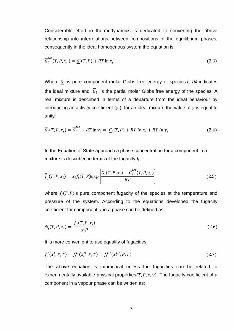
Considerable effort in thermodynamics is dedicated to converting the above
relationship into interrelations between compositions of the equilibrium phases,
consequently in the ideal homogenous system the equation is:
𝐺𝑖
𝐼𝑀(𝑇, 𝑃, 𝑥𝑖 ) = 𝐺𝑖(𝑇, 𝑃) + 𝑅𝑇 ln 𝑥𝑖 (2.3)
Where 𝐺𝑖 is pure component molar Gibbs free energy of species 𝑖, 𝐼𝑀 indicates
the ideal mixture and 𝐺𝑖 is the partial molar Gibbs free energy of the species. A
real mixture is described in terms of a departure from the ideal behaviour by
introducing an activity coefficient (𝛾𝑖); for an ideal mixture the value of 𝛾𝑖is equal to
unity:
𝐺𝑖(𝑇, 𝑃, 𝑥𝑖) = 𝐺𝑖
𝐼𝑀+ 𝑅𝑇 ln 𝛾𝑖 = 𝐺𝑖(𝑇, 𝑃) + 𝑅𝑇 𝑙𝑛 𝑥𝑖 + 𝑅𝑇 𝑙𝑛 𝛾𝑖 (2.4)
In the Equation of State approach a phase concentration for a component in a
mixture is described in terms of the fugacity fi:
𝑓𝑖(𝑇, 𝑃, 𝑥𝑖) = 𝑥𝑖𝑓𝑖(𝑇, 𝑃)𝑒𝑥𝑝 [
𝐺𝑖(𝑇, 𝑃, 𝑥𝑖) − 𝐺𝑖
𝐼𝑀(𝑇, 𝑃, 𝑥𝑖)
𝑅𝑇] (2.5)
where 𝑓𝑖(𝑇, 𝑃)is pure component fugacity of the species at the temperature and
pressure of the system. According to the equations developed the fugacity
coefficient for component 𝑖 in a phase can be defined as:
𝜙𝑖(𝑇, 𝑃, 𝑥𝑖) =
𝑓𝑖(𝑇, 𝑃, 𝑥𝑖)
𝑥𝑖𝑃 (2.6)
It is more convenient to use equality of fugacities:
𝑓�̅�𝐼(𝑥𝑖
𝐼 , 𝑃, 𝑇) = 𝑓�̅�𝐼𝐼(𝑥𝑖
𝐼𝐼 , 𝑃, 𝑇) = 𝑓�̅�𝐼𝐼𝐼(𝑥𝑖
𝐼𝐼𝐼, 𝑃, 𝑇) (2.7)
The above equation is impractical unless the fugacities can be related to
experimentally available physical properties(𝑇, 𝑃, 𝑥, 𝑦). The fugacity coefficient of a
component in a vapour phase can be written as:
8
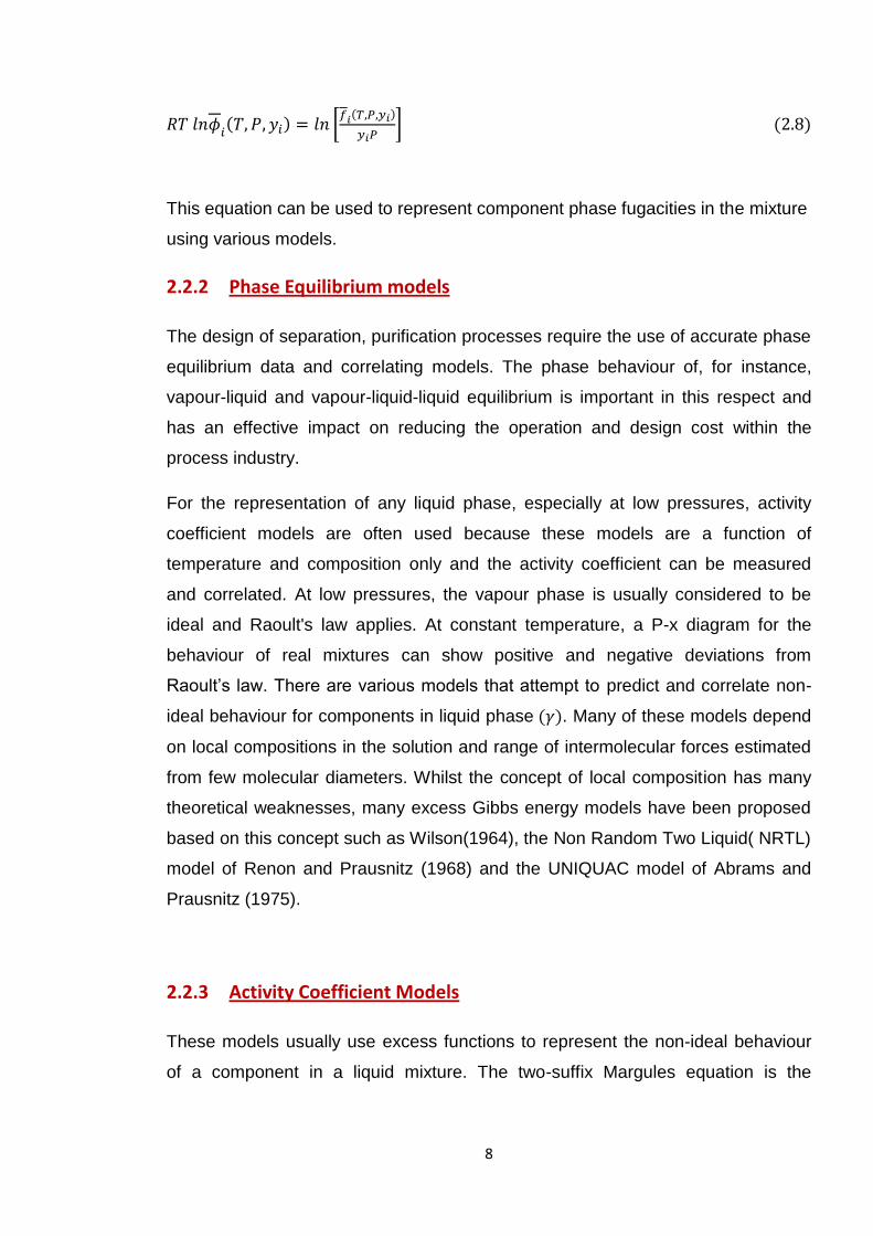
𝑅𝑇 𝑙𝑛𝜙𝑖(𝑇, 𝑃, 𝑦𝑖) = 𝑙𝑛 [
𝑓𝑖(𝑇,𝑃,𝑦𝑖)
𝑦𝑖𝑃] (2.8)
This equation can be used to represent component phase fugacities in the mixture
using various models.
2.2.2 Phase Equilibrium models
The design of separation, purification processes require the use of accurate phase
equilibrium data and correlating models. The phase behaviour of, for instance,
vapour-liquid and vapour-liquid-liquid equilibrium is important in this respect and
has an effective impact on reducing the operation and design cost within the
process industry.
For the representation of any liquid phase, especially at low pressures, activity
coefficient models are often used because these models are a function of
temperature and composition only and the activity coefficient can be measured
and correlated. At low pressures, the vapour phase is usually considered to be
ideal and Raoult's law applies. At constant temperature, a P-x diagram for the
behaviour of real mixtures can show positive and negative deviations from
Raoult’s law. There are various models that attempt to predict and correlate non-
ideal behaviour for components in liquid phase (𝛾). Many of these models depend
on local compositions in the solution and range of intermolecular forces estimated
from few molecular diameters. Whilst the concept of local composition has many
theoretical weaknesses, many excess Gibbs energy models have been proposed
based on this concept such as Wilson(1964), the Non Random Two Liquid( NRTL)
model of Renon and Prausnitz (1968) and the UNIQUAC model of Abrams and
Prausnitz (1975).
2.2.3 Activity Coefficient Models
These models usually use excess functions to represent the non-ideal behaviour
of a component in a liquid mixture. The two-suffix Margules equation is the

9
simplest function to represent the excess Gibbs energy for a binary mixture
(Prausnitz et al, 1999):
gE
𝑅𝑇= 𝑎12𝑥1𝑥2 (2.9)
where 𝑎12 is a temperature dependent adjustable parameter. The Margules
equation is applicable to mixtures with the same molecular size and shape. For
binary mixtures of molecules of different size, Wilson presented an equation for
the excess Gibbs energy as:
gE
𝑅𝑇= −𝑥1 ln(𝑥1 + Λ12𝑥2) − 𝑥2 ln(𝑥2 + 𝛬21𝑥1) (2.10)
This equation obeys the boundary conditions, that gE tends to zero as either 𝑥1 or
𝑥2tend to zero. The Wilson equation was extended by Wang and Chao (1983) in
order to increase the capability of representing partially and completely miscible
systems in calculation of VLE.
The Wilson and extended equations are not applicable to model liquid –liquid
phase equilibrium, however the Non-Random Two Liquid equation (NRTL) was
proposed by Renon(1968) which depends on a local composition concept with
three adjustable parameters(𝜏𝑗𝑖 , 𝜏𝑖𝑗) and (𝛼𝑗𝑖 = 𝛼𝑖𝑗). Equation 2.11 represents
the NRTL equation for multi-component systems:
gE
𝑅𝑇= ∑ 𝑥𝑖
𝑚
𝑖=1
∑ 𝜏𝑗𝑖𝐺𝑗𝑖𝑥𝑗𝑚𝑗=1
∑ 𝐺𝑗𝑖𝑥𝑖𝑚𝑖=1
(2.11)
Where:
𝜏𝑗𝑖 =gji − gii
𝑅𝑇 (2.12)
𝐺𝑗𝑖 = exp(−𝛼𝑗𝑖𝜏𝑗𝑖) (2.13)
The value of non-randomness parameter αji varies between 0.20 and 0.47; it is
proven that the value 0.3 can be practically used when there is a scarcity of
experimental data.

10
Abrams and Prausnitz (1975) proposed the UNIversal QUAsi Chemical
(UNIQUAC) activity coefficient model to improve the representation of excess
Gibbs energy of NRTL equation.
2.2.4 UNIQUAC
The UNIQUAC activity model is derived from the local composition theory
preserving the two parameter concept in the Wilson equation. UNIQUAC is
capable of representing partially miscible mixtures. The UNIQUAC equation
structure consists of two parts: combinatorial (the pure molecular size and shape
effects) and residual (energy interaction effects), these terms have a major impact
on the estimation of activity of the component in the mixture.
The UNIQUAC equation has been successful in correlating vapour-liquid and
liquid –liquid equilibria and it shows some superiority over Wilson, NRTL and
Margules equations for asymmetric mixtures (Thomsen et al., 2004; Rilvia et al.,
2010).
The UNIQUAC equation is used in this work to represent the Excess Gibbs Energy
of Mixing as required by the Wong Sandler Mixing Rules. More details can be
found in the theory chapter section (3.5).
2.2.5 Equation of State (EOS)
The thermodynamic properties of a substance are defined by knowing the
behaviour of the molecules in that substance. Many theories have been
suggested to describe the properties of substances; a major development in these
theories was proposed by van der Waals in 1880 arising from the corresponding-
state theory. This works on the principle that, in general, the intensive and some
extensive properties depend on intermolecular forces that are related to critical
properties in a universally applicable way. Developments from the corresponding-
states principle were initially based on a consideration of spherical molecules.
The ideal gas law fails to represent real gases under high pressure and low
temperatures. Van der Waals proposed two corrections: the parameter 𝑏 provides
a correction for the finite molecular size of gas molecules and atoms; the
parameter 𝑎 corrects for intermolecular forces. The assumptions in the ideal gas
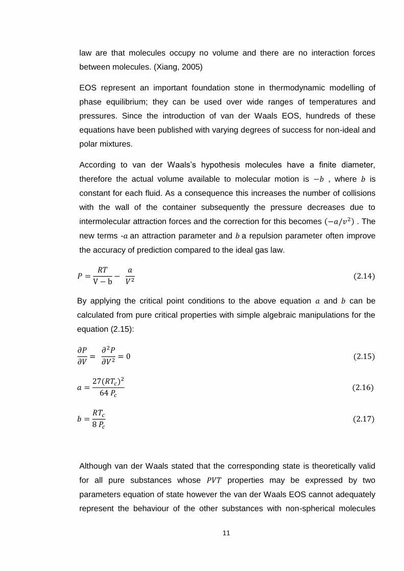
11
law are that molecules occupy no volume and there are no interaction forces
between molecules. (Xiang, 2005)
EOS represent an important foundation stone in thermodynamic modelling of
phase equilibrium; they can be used over wide ranges of temperatures and
pressures. Since the introduction of van der Waals EOS, hundreds of these
equations have been published with varying degrees of success for non-ideal and
polar mixtures.
According to van der Waals’s hypothesis molecules have a finite diameter,
therefore the actual volume available to molecular motion is −𝑏 , where 𝑏 is
constant for each fluid. As a consequence this increases the number of collisions
with the wall of the container subsequently the pressure decreases due to
intermolecular attraction forces and the correction for this becomes (−𝑎/𝑣2) . The
new terms -𝑎 an attraction parameter and 𝑏 a repulsion parameter often improve
the accuracy of prediction compared to the ideal gas law.
𝑃 =𝑅𝑇
V − b−
𝑎
𝑉2 (2.14)
By applying the critical point conditions to the above equation 𝑎 and 𝑏 can be
calculated from pure critical properties with simple algebraic manipulations for the
equation (2.15):
𝜕𝑃
𝜕𝑉=
𝜕2𝑃
𝜕𝑉2= 0 (2.15)
𝑎 =27(𝑅𝑇𝑐)2
64 𝑃𝑐 (2.16)
𝑏 =𝑅𝑇𝑐
8 𝑃𝑐 (2.17)
Although van der Waals stated that the corresponding state is theoretically valid
for all pure substances whose 𝑃𝑉𝑇 properties may be expressed by two
parameters equation of state however the van der Waals EOS cannot adequately
represent the behaviour of the other substances with non-spherical molecules

12
(polar). The deviations of these molecules are large enough to necessitate a third
parameter. The acentric factor ω suggested by Pitzer et al. (1955) obtains the
deviation of the vapour pressure-temperature relation from that expected for
substances consisting of spherically symmetric molecules (Poling et al., 2001).
The acentric factor is defined as:
𝜔 = −1.0 − log10 [𝑃𝑣𝑎𝑝(𝑇𝑟 = 0.7)
𝑃𝑐] (2.18)
Here 𝑃𝑣𝑎𝑝(𝑇𝑟 = 0.7) is the vapour pressure of the fluid at 𝑇𝑟 = 0.7 and 𝑃𝑐 is the
critical pressure.
Redlich and Kwong (RK) (1949) introduced a temperature-dependence for the
attractive term 𝑎 which improved the accuracy of van der Waals equation of
state. The RK EOS was the first equation to be productively applied to the
calculation of thermodynamic properties in the vapour phase, however it is not
considered adequate for modelling of both liquid and vapour phases.
𝑏 =𝑅𝑇
𝑣 − 𝑏−
𝑎
𝑇0.5𝑣(𝑣 + 𝑏) (2.19)
As in the van der Waals equation, the parameters 𝑎 and 𝑏 can be calculated from
critical point conditions:
𝑎 = Ω𝑎
𝑅2𝑇𝑐2.5
𝑃𝑐 (2.20)
𝑏 = Ω𝑏
𝑅 𝑇𝑐
𝑃𝑐 (2.21)
the values of Ω𝑎 and Ω𝑏 are fixed as 0.42747 and 0.0867respectively.
The success of the RK equation motivated many researchers to focus on
modification of the alpha function and predictions of volumetric properties.
(Soave, 1972; Peng and Robinson, 1976; Twu et al., 1992). Wilson (1964, 1966)
introduced a general form of the 𝑎 parameter and expressed the 𝛼(𝑇) as a
function of the temperature and the acentric factor:
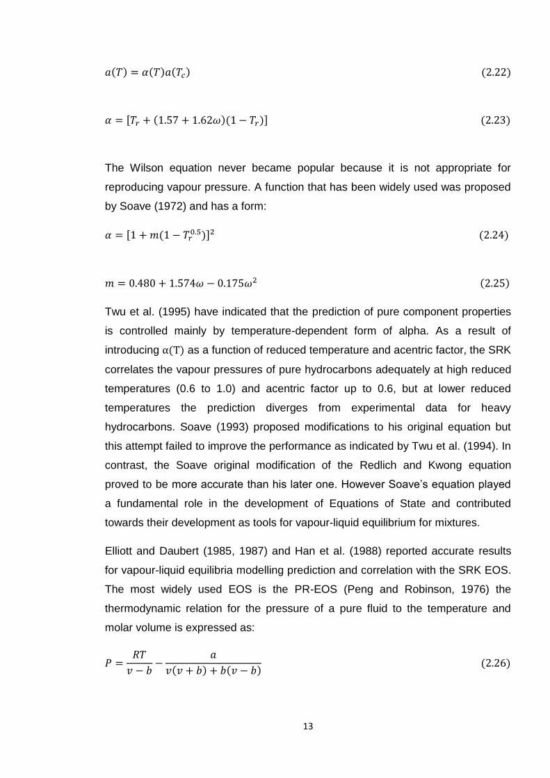
13
𝑎(𝑇) = 𝛼(𝑇)𝑎(𝑇𝑐) (2.22)
𝛼 = [𝑇𝑟 + (1.57 + 1.62𝜔)(1 − 𝑇𝑟)] (2.23)
The Wilson equation never became popular because it is not appropriate for
reproducing vapour pressure. A function that has been widely used was proposed
by Soave (1972) and has a form:
𝛼 = [1 + 𝑚(1 − 𝑇𝑟0.5)]2 (2.24)
𝑚 = 0.480 + 1.574𝜔 − 0.175𝜔2 (2.25)
Twu et al. (1995) have indicated that the prediction of pure component properties
is controlled mainly by temperature-dependent form of alpha. As a result of
introducing α(T) as a function of reduced temperature and acentric factor, the SRK
correlates the vapour pressures of pure hydrocarbons adequately at high reduced
temperatures (0.6 to 1.0) and acentric factor up to 0.6, but at lower reduced
temperatures the prediction diverges from experimental data for heavy
hydrocarbons. Soave (1993) proposed modifications to his original equation but
this attempt failed to improve the performance as indicated by Twu et al. (1994). In
contrast, the Soave original modification of the Redlich and Kwong equation
proved to be more accurate than his later one. However Soave’s equation played
a fundamental role in the development of Equations of State and contributed
towards their development as tools for vapour-liquid equilibrium for mixtures.
Elliott and Daubert (1985, 1987) and Han et al. (1988) reported accurate results
for vapour-liquid equilibria modelling prediction and correlation with the SRK EOS.
The most widely used EOS is the PR-EOS (Peng and Robinson, 1976) the
thermodynamic relation for the pressure of a pure fluid to the temperature and
molar volume is expressed as:
𝑃 =𝑅𝑇
𝑣 − 𝑏−
𝑎
𝑣(𝑣 + 𝑏) + 𝑏(𝑣 − 𝑏) (2.26)

14
In equation (2.26) the co-volume parameter 𝑏 is considered independent of
temperature while 𝑎 depends on temperature to reproduce vapour pressure, for
pure component 𝑎 is specified by:
𝑎 = 𝛼(𝑇)𝑎(𝑇𝑐) (2.27)
Peng and Robinson calculated the first and second isothermal derivatives of pure
substance pressure with respect to volume by van der Waals and solved equation
(2.26) for parameters 𝑎(𝑇𝑐) and 𝑏:
𝑎(𝑇𝑐) = 0.45724(𝑅𝑇𝑐)2
𝑃𝑐 (2.28)
𝑏 = 0.07780𝑅𝑇𝑐
𝑃𝑐 (2.29)
Where:
𝛼(𝑇) = {1 + 𝑚 [1 − √𝑇
𝑇𝑐]}
2
(2.30)
𝑚 = 0.37464 + 1.5432𝜔 − 0.26992𝜔2 (2.31)
Stryjek and Vera (1986) modified the attraction term of PR-EOS by introducing the
adjustable pure component parameter 𝑘1 and changing the 𝑘0 polynomial fit to
power 3 of the acentric factor:
𝑘 = 𝑘0 + 𝑘1(1 + √𝑇𝑟)(0.7 − 𝑇𝑟) (2. 32)
𝑘0 = 0.378893 + 1.4897153𝜔 − 0.17131848𝜔2 + 0.0196554𝜔3 (2.33)
The parameter 𝑘1 is obtained by fitting the saturation pressure versus temperature
data for a pure component. In their subsequent modification Stryjek and Vera
(1986) added two additional pure parameters in an attempt to improve PR-EOS for
polar molecules. The last modified version of PR-EOS is PRSV2; this differs from
the previous modification in that the expression used for 𝑘 in equation (2.32) and
the 𝑘 proposed for PRSV2 takes the following form:
15
𝑘 = 𝑘0 + [𝑘1 + 𝑘2(𝑘3 − 𝑇𝑅)(1 − 𝑇𝑅0.5)](1 + 𝑇𝑅
0.5)(0.7 − 𝑇𝑅) (2.34)
The 𝑘1 , 𝑘2 𝑎𝑛𝑑 𝑘3 are pure component adjustable parameters and their values for
some components can be found in Stryjek and Vera (1986). The use of additional
parameters does not have significant impact on improving the pure component
vapour pressure calculation; however the main emphasis is on the type of mixing
rules used in VLE correlation for non-ideal mixtures.
Hinojosa-Gomez et al. (2010) presented two modifications of the Peng Robinson
EOS. The first method enhanced the EOS pure component property predictions
whilst the second alteration proposed a temperature dependency for 𝑏 the
repulsive parameter. A test was carried out by Hinojosa-Gomez et al. (2010) for 72
pure substances including highly polar compounds and the results were in
significant agreement with experimental data. Many researchers have conducted
comparative studies in an attempt to identify the best EOS for predicting
thermodynamic properties for pure components. Nasrifar (2010) examined eleven
equations of state for predicting hydrogen properties at temperatures greater than
200 K and almost all the results are comparable in accuracy.
Different approaches have been proposed by many researchers in an attempt to
improve the 𝛼 function in equation 2.27 for heavy hydrocarbons and polar
substances. Carrier et al. (1988) and Rogalski et al. (1990) developed a method
in conjunction with the Peng-Robinson EOS. In contrast to the 𝛼 function, the
repulsive parameter 𝑏 is generally kept independent of temperature. However the
main purpose in using an Equation of State (EOS) is a representation of mixture
properties and the basic quadratic mixing rules can be assumed from the
composition dependence of the two main parameters (𝑎, 𝑏) of EOS. The common
assumption that the same EOS used for pure fluid can be applied for mixtures is
expanding the EOS in virial form, for Peng Robinson EOS one obtains:
𝑃𝑉
𝑅𝑇= ∑ (
𝑏
𝑉)
𝑛
−𝑎
𝑅𝑇𝑉+
2𝑎𝑏
𝑅𝑇𝑉2+ ⋯
∞
𝑛=0
(2.35)
16
2.3 Mixing Rules
2.3.1 Van der Waals Mixing Rules
Cubic equations of state (EOS) have been used in the process industries for
calculation of phase equilibrium. In order to extend the use of the EOS form pure
components to mixtures, the 𝑎 , 𝑏 functions must be adjusted for mixtures.
Equation (2.35) provides a limit that mixing rules parameters should obey; this is
known as the one fluid van der Waals mixing rules 1PVDW:
𝑎 = ∑ ∑ 𝑥𝑖𝑥𝑗𝑎𝑖𝑗
𝑗𝑖
(2.36)
𝑏 = ∑ ∑ 𝑥𝑖𝑥𝑗𝑏𝑖𝑗𝑗𝑖 (2.37)
𝑎𝑖𝑗 = (𝑎𝑖𝑖𝑎𝑗𝑗)1
2(1 − 𝑘𝑖𝑗) (2.38)
𝑏𝑖𝑗 =1
2(𝑏𝑖𝑖 + 𝑏𝑗𝑗)(1 − 𝑙𝑖𝑗) (2.39)
where 𝑘𝑖𝑗 and 𝑙𝑖𝑗 are the binary interaction parameters obtained by fitting the
model to experimental data. Generally 𝑙𝑖𝑗 is set to zero, in this case equation
(2.37) is simplified to:
𝑏 = ∑ ∑1
2 𝑥𝑖𝑥𝑗(𝑏𝑖𝑖 + 𝑏𝑗𝑗)
𝑗𝑖
(2.40)
The classical quadratic mixing rules are, in general, appropriate for the
representation of VLE phase equilibrium in multicomponent systems containing
nonpolar and weakly polar components. Testing the performance of different EOS
and obtaining similar results indicates that the mixing rules are more important
than the actual mathematical relationship of (𝑃, 𝑉, 𝑎𝑛𝑑 𝑇) embodied in an EOS. An
empirical attempt to overcome the weaknesses of the 1PVDW additional
composition dependence has been introduced to the 𝑎 parameter of EOS
(2PVDW).The extra parameter considered has improved the capabilities of van

17
der Waals mixing rules for representing VLE data of non-ideal systems that could
not be correlated with 1PVDW.
Orbey and Sandler (1998) tested 1PVDW and 2PVDW predictions for VLE
calculations on several binary systems; they concluded that the 1PVDW fluid
model is not accurate for the description of the phase equilibria of some simple
hydrocarbon/water (i.e. acetone/water) mixtures. However the accuracy of the
results using 2PVDW is in contrast with the 1PVDW mixing rules.
Several researchers have proposed new mixing rules by combining the EOS and
the activity coefficient models.
2.3.2 Huron and Vidal Mixing Rules (HVMR)
Huron and Vidal (1979) verified that the van der Waals mixing rules are reliable in
representing a mixture of hydrocarbons but incapable for polar components. They
developed a technique that matches the excess Gibbs energy GE derived from an
equation of state with that from an activity coefficient model at infinite pressure.
Their combination produced a mixing rule with the parameter 𝑎 expressed as in
following equation:
𝑎 = 𝑏 [∑ 𝑥𝑖 (𝑎𝑖
𝑏𝑖) +
𝐺𝐸
𝐶∗] (2.41)
𝑏 is as expressed in equation (2.40) , 𝐶∗is a parameter for EOS, for PRSV EOS is -
0.62323. The novelty of Vidal and Huron’s innovation has motivated a number of
authors to develop several EOS/GE models. To further develop these models to be
totally predictive, the UNIFAC activity coefficient was introduced instead of
empirical models.
In order to improve the HVMR model for low pressure systems using the UNIFAC
predictive model, the excess free energies should be matched at zero pressure. In
this procedure the molar volume of liquid species must be found from EOS and to
solve this problem Michelsen (1990) developed an extrapolation method to
approximate the molar volume at zero pressure. This modification evolved into a
series of HVMRs so called MHV1, MHV2 and a linear combination of Huron-Vidal
and Michelsen (LCHVM).

18
For some non-ideal mixtures Huron and Vidal mixing rules HVMR are shown to be
superior to both 1PVDW and 2PVDW MRs, but not satisfactory for VLE correlation
over a wide range of temperatures as observed by Orbey and Sandler (1998).
One of the major shortcomings of HVMRs is that the excess Gibbs free energy is
independent of pressure and does not satisfy the requirement that the second
virial coefficient is a quadratic function of composition (Ghosh and Taraphdar,
1998) consequently this mixing rule cannot be used for the calculation of VLE for
highly asymmetric systems.
2.3.3 Wong Sandler Mixing Rules
Wong and Sandler (1992) proposed a Mixing Rule (WSMR) by combining the
excess Gibbs free energy models and equation of state. WSMR provides an
alternative approach for developing mixing rules as proposed by Huron and Vidal
(1979). Wong and Sandler assumed the Helmholtz free energy 𝐴𝐸 is relatively
insensitive to pressure and this could be used in their mixing rules [𝑎𝑠 𝐺𝐸(𝑥)
expression at low pressure]. They considered equating the excess Helmholtz free
energy at infinite pressure from an EOS to that of an activity coefficient model; the
assumption is:
𝐴∞𝐸
𝑅𝑇=
𝐺𝐸(𝑥)
𝑅𝑇 (2.42)
The parameter 𝑎 from any EOS is related to the attractive term 𝑏 through the
relation:
𝐵(𝑇) = 𝑏 −𝑎
𝑅𝑇 (2.43)
From statistical mechanics the term (𝑏 −𝑎
𝑅𝑇) for the mixture is written as:
(𝑏 −𝑎
𝑅𝑇) = ∑ ∑ 𝑥𝑖𝑥𝑗 (𝑏 −
𝑎
𝑅𝑇)
𝑖𝑗 (2.44)
The 𝑥 is composition and the term (𝑏 − 𝑎/𝑅𝑇)𝑖𝑗 is composition–independent from
EOS is given by:
19
(𝑏 −𝑎
𝑅𝑇)
𝑖𝑗=
(𝑏 −𝑎
𝑅𝑇)𝑖𝑖
+ (𝑏 −𝑎
𝑅𝑇)𝑗𝑗
2(1 − 𝑘𝑖𝑗) (2.45)
𝑘𝑖𝑗 is binary interaction parameter and 𝑘𝑖𝑖 = 𝑘𝑗𝑗 = 0
Coutsikos et al.(1995) indicated that the 𝑘𝑖𝑗 can be determined either by equating
the 𝐺𝐸 from an equation of state (at P=1 bar , system temperature, 𝑥 = 0.5 ) to that
from an activity coefficient models or by fitting the VLE data using minimisation
function (Average Absolute relative Deviation AAD in bubble point pressure plus
the AAD in the vapour phase mole fraction). However they preferred the VLE
predictions for symmetric and asymmetric systems using WSMR with the 𝑘𝑖𝑗 value
obtained from the correlation of VLE data, as they identified the inability of a
composition-independent 𝑘𝑖𝑗for asymmetric mixtures. Orbey and Sandler (1995 a)
proposed a slightly reformulated version of the original WS mixing rule in which
they retained the main concept but changed the combining rule of equation (2.45)
to the following equation:
(𝑏 −𝑎
𝑅𝑇)
𝑖𝑗=
1
2(𝑏𝑖 + 𝑏𝑗) −
√𝑎𝑖𝑎𝑗
𝑅𝑇(1 − 𝑘𝑖𝑗) (2.46)
This mixing rule has been successful and widely used in the way that an activity
coefficient model can be combined with any EOS to represent vapour pressure.
The good correlations of vapour-liquid, liquid-liquid and vapour-liquid-liquid
equilibria for WSMR as shown by Orbey and Sandler (1998) led them to a
conclusion that this mixing rule can be expanded to a wide range of applications
which previously could only be correlated with activity coefficient models. When
there is an absence of VLE data, this model can be completely predictive with
infinite dilution activity coefficients obtained from the UNIFAC model. (Orbey
Sandler, 1995a).
Ghosh and Taraphdar (1998) have used PRSV combined with Wong Sandler
mixing rules through NRTL activity model for the VLE prediction of forty-three
binary mixtures from various ranges of organic, esters, ketones. Their results are
comparable to those reported in the DECHEMA data series.
20
In a comparative study of several mixing rules for EOS in the prediction of multi-
component VLE, several mixtures consisting of a polar component (Ethanol) ,
moderately polar(Chloroform) , Hexane which represents non-polar component
and Acetone which is a highly polar component, were selected in their work.
Bazua et al. (1996) showed that in most cases Wong Sandler mixing is the most
effective among 22 mixing rules.
There have been several attempts to combine an EOS with a predictive activity
coefficient model using an indirect approach. Lee and Lin (2007) reported
successful VLE and LLE predictions for highly non ideal mixtures in a wide range
of temperature and pressure using PR-EOS combined with a predictive liquid
model the Conductor-like Screening Model - Segment Activity Coefficient
(COSMO-SAC) through WS mixing rules. They also recommended the WSMR
among the best of three different mixing rules. Khodakarami et al. (2005) indicated
that the PRSV +WSMR is suitable for the calculation of VLE for strongly non-ideal
mixtures, they reached this conclusion by examining the WSMR on several binary
and ternary systems. However in the following paper, Lotfollahi et al. (2007) have
shown in their proposed predictive method, that the value of the interaction
parameter 𝑘12 can be evaluated directly without the availability of VLE
experimental data.
Some researchers have taken the problem a step further by correlating a VLLE
model for reactive distillation. Hsieha et al. (2011) conducted a study of multiphase
equilibria for mixture and measured experimental VLLE data for a ternary system
(water, isopropanol, and isopropyl propionate). They utilised Soave-Redlich-
Kwong EOS with Wong-Sandler mixing rule. They agreed on the improvement of
the accuracy of the VLLE flash calculation when the parameters of the activity
models were determined from the ternary rather than the parameters obtained
from binaries VLLE.
Mario and Mauricio (2011) have shown that the PRSV2+UNIQUAC+WS model is
capable of correlating the experimental VLE data at 200oC for ethylene –water,
ethylene-ethanol and ethanol-water and predicting the VLE of ethylene-water-
ethanol ternary system at the same temperature and various pressures.

21
2.4 Optimisation methods for phase equilibrium modelling
Reliable phase equilibrium modelling is essential for design, simulation and
operation of the separation processes. The precise description of phase behaviour
of a mixture has a substantial impact on the design plan and the energy costs of
operation of any chemical industry process. According to thermodynamic
prediction a mixture at specific Temperature (𝑇) and Pressure (𝑃) with overall
composition (𝑧) will split to a 𝑛 number of stable phases at equilibrium.
The optimisation problem for non-reactive systems can be expressed as follows:
minimise 𝐹(𝑦) subject to material balance constraints. At equilibrium the fugacities
of each component are equal in all the phases. The classical approach is equality
of fugacities (K-values) and mass balance. These conditions are not sufficient to
calculate phase equilibrium particularly in multi-phase multi-component polar
systems. It is essential that the Gibbs free energy of mixing will be at the minimum
level possible. A global minimisation is required for solving the mathematical
problem of phase equilibrium modelling as many optimisation methods fail to
converge to the real solution due to a highly non-linear objective function with
many local optima and many decision variables.
Generally there are two approaches to solve phase equilibrium problems as
pointed out by Iglesias-Silva et al. (2003):
1. solving simultaneously the material balance and thermodynamic equations
(K-value method).
2. Gibbs free energy minimisation methods. The traditional optimisation
methods may fail to converge to the correct solution when the initial values
are not close to the real solution, in the area of phase boundaries and in the
critical region.
2.4.1 Equation solving method
The equation solving approach is a classical method of searching for solutions for
phase equilibrium calculations. This method requires a good initial estimate if an
22
iterative calculation is used (Newton method). Michelsen (1993) indicated that in
the absence of a good initial estimate, the iterations may converge to trivial
solutions especially in the phase boundaries and critical regions.
This method usually consists of solving a system of non-linear and non-convex
equations simultaneously which are obtained from the Gibbs free energy
optimisation and the mass balances. Some computational difficulties are expected,
such as convergence and initial estimates which may produce multiple solutions;
in order to guarantee obtaining global solutions a convexity analysis is required.
(Teh & Rangaiah, 2002; Lin & Stadtherr, 2004; Rossi & et al., 2011)
2.4.2 Direct minimisation techniques
A reliable and accurate method for global optimisation is desired for
thermodynamic phase calculations; due to the non-linearity and complexity of the
Gibbs free energy function. The development of global optimisation methods
played a significant role in modelling phase equilibria of multi-component multi-
phase systems. Since the Michelsen's Tangent Plane Criterion for Gibbs free
energy minimisation, many deterministic and stochastic global methods have been
used in phase equilibrium computations. The global optimisation problems are a
challenging task because the objective functions are highly non-linear and non-
convex, the complexity increases when an EOS is used for modelling
thermodynamic properties for all the phases at equilibrium. Many researchers
have indicated the same problem with the objective function for parameter
estimation specifically for VLE and VLLE modelling for multi-component systems
as the non-differentiable objective function may converge to a local minimum. This
will have significant impact on phase equilibrium calculations and predictions. This
will cause uncertainties in design processes. Several studies have emphasized the
need for reliable global optimisation techniques. (Bollas et al., 2009; Bonilla-
Petriciolet et al., 2010). Global optimisations can be classified into deterministic
and stochastic methods.
23
2.4.2.1 Deterministic methods
Deterministic approaches take advantage of the analytical properties of the
mathematical problem to generate a deterministic sequence of points where each
point of the sequence does not depend on the value of the objective function at
previous points. This method relies on a grid search to converge to a global
solution. In their conclusions Lin et al. (2012) have found that stochastic
approaches are more flexible and efficient than deterministic approaches.
The different deterministic global optimisation approaches applied to phase
equilibrium calculations and modelling are mainly:
1. Branch and Bound Global Optimisation
This method adapts partition strategies, sampling and lower and upper bounding
procedures in finding global solutions.
2. Homotopy Continuation Methods
This method is described by continuously constructing a simpler problem from the
given one, and then gradually deforming into the original one while solving the
constructed simpler problem.
3. Interval analysis
This is a computational method to solve nonlinear equations using interval vectors
and matrices starting with an initial interval value and searching all the roots by
solving a linear interval equation system for a new interval value.
These methods in general are often slow and require significant numerical
calculations that increase proportionally with the problem size; a reasonable and
wide initial interval should be provided to converge to a global solution rather than
a local minimum. (Zhang et al., 2011)
Deterministic approaches have been used to solve the global stability problem.
Sun & Seider (1995) used the Newton homotopy-continuation method to
determine phase equilibria for some hydrocarbon mixtures by minimising global
Gibbs free energy. McDonald & Floudas (1997) successfully applied the branch
and bound method calculating Gibbs free energy for a number of hydrocarbon

24
systems. The Newton-interval method is used by Burgos-Solorzano et al. (2004) in
the calculation of phase equilibria for high pressure multi-phase systems.
The Area Method was developed by Eubank et al. (1992) and later tested by
Hodges et al. (1997) on VLE, LLE VLLE binary systems. It is an example of a
deterministic optimisation method and utilises a grid search to find a maximum
positive net area confined by the Gibbs energy surface (𝜙) and the tangent plane
to the surface. Hodges et al. (1998) attempted to extend the area method for
ternary multi-phase calculations; this was in fact, a volume method which was not
successful. As an alternative approach they developed a Tangent Plane
Intersection method. More explanation of this method is given in the theory
chapter, section (3.10.2).
2.4.2.2 Stochastic method
Stochastic optimisation uses probabilistic elements and random sequences in the
search for global optimum (Rangaiah et al., 2011). In this method new techniques
are used such as diversification (explore regions that have not been searched),
intensification (provides a simple method to focus the search around the current
best solution) and learning strategies to find solutions. In the last two decades,
there has been a significant interest in developing reliable optimisation techniques
for Phase Equilibrium Calculations (PEC).
Henderson et al. (2001) indicated that emphases were focused on methods which
used less computational effort in comparison with deterministic approaches. The
main advantages of using stochastic optimisation are: they are applicable to any
structures of the problem; require only calculations of objective function and can
be used with all thermodynamic models. To date a number of stochastic
optimisations have been studied for example:
1. Pure Random Search (PRS) used by Lee et al. (1999) and Adaptive
Random Search (ARS) uses random search points and a systematic region
reduction strategy to locate the global optimum value for the objective
function. (Luus & Rangaiah, 2010).

25
2. Harmony Search (HS): this algorithm was devised by Geem et al. (2001)
using the analogy of the music performance process. The advantageous
features of this search are ; makes new vectors by considering all existing
vectors, the HS does not require the initial values decision variables, can
solve continuous-variables as well as combinatorial problems and can be
applied to various fields.
3. Simulated Annealing (SA): was developed by Kirkpatrick et al. (1983). SA is
an attempt to mimic the physical phenomenon of annealing in which a solid
is first melted and then allowed to cool by decreasing the temperature.
During the cooling process the particles form a structure of minimum
energy. From a mathematical point of view the SA search process for
optimum is through the adaptive acceptance/rejection criterion of the lowest
energy points. Various forms of SA have been proposed and applied for
phase equilibrium calculations.(Rangaiah, 2001; Zhu et al., 2000 ; Bonilla-
Petriciolet et al., 2007)
4. Genetic Algorithm (GA): The main concepts of this algorithm are; survival of
the fittest, crossover and mutation operations for generating new
individuals. The search starts with initializing of a population which are
generated randomly. The objective function is evaluated for the population
in the first iteration then the individuals undergo reproduction, crossover
and mutation. In the reproduction process more copies of the fittest will
meet. The crossover allows the algorithm to escape from local minima. In
this procedure new individuals are formed and after mutation the new
population is created. This process is repeated until the stopping criteria are
satisfied. The GA is widely used in chemical engineering and phase
equilibria. (Alvarez et al., 2008; Babu et al., 2009)
5. Tabu Search (TS): This method was developed by Glover (1989) The Tabu
means that the algorithm should not re-visit the points which have been
searched previously. For creating new points, this algorithm compares the
current values with the previous search, lists the worst points in the taboo
list and creates a strategy to search in new regions. (Teh & Rangaiah,
2003; Lin & Miller, 2004)
26
6. Particle Swarm Optimisation (PSO): this algorithm exploits the behaviour of
a biological social system of a flock of birds or a school of fish in search for
global optimum. PSO consists of a number of particles; each particle has a
potential impact on the global solution in the search space. The particles do
not recombine directly between each other; they behave socially according
to the personal best and the global best positions in the swarm instead. The
search strategy allows the particles to stochastically move to the best
region in the search space. PSO has been applied successfully in phase
stability and phase equilibrium calculations. (Rahman et al., 2009; Zhang et
al., 2011)
2.4.2.3 Nelder-Mead
Nelder–Mead is a direct search method widely used in the field of chemical
engineering and phase equilibrium calculations. This method optimises non-linear,
multi-variable and unconstrained function by using only the function value. The
main advantages for using this simplex are; implicitly, no derivatives of function
are required. For each of the iterations the search starts with a set of new
variables which are generated depending on the coefficient factor values
(reflection, expansion, contraction and shrinkage). The search for new variables
terminates when the function is at optimum value.
The Nelder-Mead simplex is used through this research to minimise constrained
functions (for VLE, LLE, VLLE and Gibbs free energy). The simplex is restricted
to search in a required range and this is achieved by giving the function a penalty
when the variable values generated are outside the desired range.
Hodges et al. (1998) have demonstrated the applicability of the Tangent Plane
Intersection (TPI) for calculations of binary and ternary multiphase equilibrium. The
Nelder Mead simplex was used as a minimisation method and in their search
procedure local optimum values were found by grouping the variables into two
different groups they called this (hybrid1 and hybrid2). The process then
conducted an extra plus and cross search near the located values in case these
methods failed to find the zero solution for the objection function.
27
2.4.3 Other method of phase equilibrium calculations (reduced variables)
The reduced variables method was presented by Michelsen (1986); he proved that
the phase equilibrium model could be expressed mathematically in terms of three
independent variables. The number of variables does not depend on the number
of components in the mixture. Michelsen's approach was limited to zero Binary
Interaction Coefficients (BIC) parameters in the Peng Robinson EOS. Several
researchers developed Michelsen’s method for selecting independent variables
without restricting the number of non-zero BICs (Hendriks & van Bergen, 1992;
Nichita & Minescu, 2004).
The theoretical concept of the reduction method is to express the fugacity
coefficients as a function of a reduced number of variables, instead of expressing
them as a function of composition. This method is particularly efficient for mixtures
with many components and few non-zero BICs such as hydrocarbon systems in oil
reservoirs where most BICs are between hydrocarbon molecules in the
homogeneous phase and are set to zero (Nichita and Graciaa, 2011).
Nichita et al. (2006) used the reduction method in a combined phase stability
analysis and phase splitting procedure to model the phase equilibrium of
asphaltene precipitation from oil and also on a sour gas system. They used two
cubic EOS; SRK and PR-EOS and claimed their method was robust and efficient.
2.5 The Problem of Initialisation in Phase Equilibria Calculations
In phase equilibrium calculations for heterogeneous multi-phase mixtures
regardless of the method used, good initial estimate values are required. Three
phase split calculation starts by the mathematically formulating of two sets of
equations. The first set describes the equilibrium conditions through the fugacity
coefficient ratios so called 𝐾𝑖 factors. The second set is the material balance
description known as Rachford-Rice (RR) equation. The most efficient approaches
in solving the two sets of equations are: equations solving method using
deterministic algorithm such as Newton method, and Gibbs free minimisation
method.
28
It has been proven that in the presence of a poor initial estimate it is possible that
the optimisation converges to a trivial solution. Many researchers have indicated
that this problem is due to non-convex non-linear properties of the objective
function with several local minima. (Michelsen, 1982 a; Green et al., 1993;
McDonald and Floudas, 1995; Nichita et al., 2002; Teh & Rangaiah, 2002;
Leibovici, 2006; Li and Firoozabadi, 2012).
Michelsen (1982 a) observed the effect of initial estimates on flash calculations
and in an attempt to improve the reliability of locating the stationary points, he
used multiple initial points. Michelsen used the Wilson correlation for low pressure
calculations in VLE of hydrocarbon systems and he suggested that the results of a
stability test can be used as an initial estimate in flash calculation procedures
especially when the Newton-Raphson method is utilised.
Teh and Rangaiah (2002) have applied a Simultaneous Equation Solving (SES)
approach in modelling phase equilibria for a series of VLE, LLE and VLLE binary
and multicomponent systems. They clearly indicated the issue of convergence to
a trivial solution in absence of a good initial estimate especially in the phase
boundaries and critical regions.
In their proposal, Haugen and Firoozabadi (2011) used a two-dimensional
bisection method in the first iteration of a Successive Substitution Iteration (SSI)
loop to obtain a good initial estimate for the Newton algorithm used to solve the
three phase split calculations using the Rachford-Rice equations. They pointed
out that this problem is due to the lack of an initial estimate for the phase fraction
for the first iteration of the successive substitution, particularly when these
estimates come from a correlation or from stability analysis. Their method of
initialisation based on the two-phase stability analysis test results can be used as
a good initial estimate for three- phase equilibria computation.
The contributing factors used in selecting the type of initialisation approach are:
the system conditions, complexity of the system (polarity or the level of non-
ideality) to be modelled and the type of algorithms used in the minimisation of
Gibbs free energy. In general there are two types of initialisation methods found
in the literature. The methods are independent of compositions that use Wilson’s
proposed approximation (eq. 2.48) and methods are depending on composition.
29
2.5.1 Initialisation method for VLE calculations
Phase stability analysis was first set by Gibbs and subsequently formulated by
Michelsen (1982 a) in the term of the Tangent Plane Distance Function TPDF, the
function to be minimised globally is: (more details on TPDF can be found in Theory
chapter section (3.10.4))
𝑇𝑃𝐷𝐹(𝑌) = ∑ 𝑌𝑖[(𝑙𝑛𝑌𝑖 + 𝑙𝑛𝜙𝑖(𝑌) − ℎ𝑖)]𝑛𝑐𝑖 (2.47)
𝑤ℎ𝑒𝑟𝑒 ∶ ℎ𝑖 = 𝑙𝑛𝑧𝑖 + 𝑙𝑛𝜙𝑖(𝑧)
Where 𝑌𝑖 is trial phase composition for component 𝑖 and subject to: ∑ 𝑌𝑖 = 1 and
0 ≤ 𝑌𝑖 ≤ 1 . At low pressure the 𝐾-factor is expressed approximately by Wilson
correlation:
𝐾𝑖 =𝑃𝐶𝑖
𝑃𝑒𝑥𝑝 {5.3727(1 + 𝜔𝑖) (1 −
𝑇𝐶𝑖
𝑇)} (2.48)
Michelsen used two sets of initial estimates: (𝑌𝑖 = 𝐾𝑖𝑧𝑖) & (𝑌𝑖 = 𝐾𝑖/𝑧𝑖) in the
minimisation of the TPDF objective function for VLE flash calculation of low
pressure hydrocarbon systems.
Michelsen also used a different initialisation approach for high pressure systems
which is based on the decreasing monotonic function 𝐹(𝑉) which provides
assumptions for initial estimates of liquid mole fraction in VLE phase calculations.
However the high pressure systems are not in the scope of this research.
A simple initialisation method is proposed by Leibovici (2006) for VLE flash
calculation on hydrocarbon mixtures in oil and gas reservoir simulation. The initial
values of equilibrium constants (𝐾𝑖) are estimated from: 𝐾𝑖 = 𝑃𝑖𝑠𝑎𝑡/𝑃 where the
saturation pressure of pure component is calculated using an equation of state at
the system temperature. The next step computes the infinite dilution fugacity
coefficients for all the components in the vapour and liquid phases. The new
values of equilibrium constants are generated 𝐾𝑖0 = 𝜑𝑖
𝐿/𝜑𝑖𝑉 , the final step is
correcting the (𝐾𝑖) value according to 𝐾𝑖 = 𝐾𝑖0(
𝑃𝑖𝑠𝑎𝑡
𝑃) .
30
2.5.2 Initialisation method For LLE calculations
Trebble (1989) suggested an initialisation scheme similar to that used in the VLE
initiation, by assuming the first liquid phase compositions
𝑥𝑖𝐿1 equal to overall feed composition. The second liquid phase compositions
generated by an equation similar to that described by Michelsen (1982 b) for
stability analysis:
𝑙𝑛 𝑥𝑖𝐿2 = 𝑙𝑛𝑥𝑖
𝐿1 + 𝑙𝑛𝜙𝑖(𝑥𝐿1) − 𝑙𝑛𝜙𝑖𝑜 (2.49)
The author indicated the possibility of the trivial solution in LLE iterations due to
small differences between the fugacity of the component in the mixture and pure
liquid fugacity(𝜙𝑖𝑜). In order to solve this issue he suggested resetting the
equilibrium ratio 𝐾𝑖 values in the range (1.0 - 2.0) to a value of 2.0 and to a value
0.5 in the range of (0.5-1.0) (Trebble 1989).
Bonilla-Petriciolet (2007) introduced an initialisation strategy for the Equal Area
Rule (EAR) in flash calculations on LLE ternary systems. EAR is Gibbs free
energy minimisation method suggested by Eubank and Hall (1995) which uses an
integrative approach in the search for equilibrium composition. Bonilla-Petriciolet
uses the results obtained from the global optimisation of TPDF as a good initial
estimate to calculate the tie-line vector in an attempt to improve the numerical
behaviour of the EAR algorithm and produce easy convergence. The author
applied this initialisation technique on modelling liquid -liquid equilibrium for three
ternary and one hypothetical ternary system using Soave-Redlich-Kwong EOS
with classical mixing rules and the Margules equation.
Teh and Rangaiah (2002) have used the procedure of Ohanomah and Thompson
(1984) in estimating the initial values for the LLE calculation on six systems (3
binaries, 3 ternaries) using three Activity Coefficient Models (UNIQUAC, NRTL
and UNIFAC). Their procedure is based on replacing the multi-component mixture
by a hypothetical binary system, then identifying the extract solvent (lowest 𝐾𝑖 )
and the raffinate solvent (highest 𝐾𝑖) . The steps are listed below:
1. Set 𝑥𝑖𝐿1 = 𝑧𝑖, calculate 𝛾𝑖
𝐿1 and then 𝑥𝑖𝐿2 = 𝑧𝑖 𝛾𝑖
𝐿1.
2. Normalise 𝑥𝑖𝐿2, calculate 𝛾𝑖
𝐿2 and then 𝐾𝑖 = 𝛾𝑖𝐿1/𝛾𝑖
𝐿2.

31
3. Identify the component with the lowest and highest 𝐾𝑖 value and their feed
compositions are then donated as 𝑧𝑅 and 𝑧𝐸 ,where 𝑅 and 𝐸 raffinate and
extracted respectively.
4. Set 𝑥𝑅𝐿1 = 𝑥𝐸
𝐿2 = 0.98 and 𝑥𝐸𝐿1 = 𝑥𝑅
𝐿2 = 0.02 , revaluate 𝐾𝐸 = 𝑥𝐸𝐿2/𝑥𝐸
𝐿1 and
𝐾𝑅 = 𝑥𝑅𝐿2/𝑥𝑅
𝐿1.
5. Finally, calculate the initial estimate for the second liquid phase split :
𝜃𝐿2 = [𝑧𝐸 (1 −1
𝐾𝐸) + 𝑧𝑅 𝐾𝑅] (𝑧𝐸 + 𝑧𝑅) .
2.5.3 Initialisation method for VLLE calculations
The main focus in the literature on the prediction of multiphase equilibrium flash
calculations is the reliability of the algorithms. Convergences of these algorithms
depend on the initial values of compositions of each component between different
phases. The methods of generation of initial estimates for VLLE of polar systems
in the literature are given uneven treatment. A few researchers have implemented
the Wilson approximation (𝐾𝑖) for non-polar hydrocarbon mixtures. Pan and
Firoozabadi (2003) used both the Wilson equation and stability test in VLE
calculations. They observed that the Wilson approximation increases the number
of iterations and at high pressure often lead to a single phase in comparison with
using the stability test method in initial estimation methods.
In a comparison study by between the equation solving method and Gibbs free
energy minimisation for phase equilibrium calculation, Teh and Rangalah,(2002)
applied the Trebble VLLE initialisation scheme (Trebble, 1989). Their procedure
depends on the assumption that the first liquid composition set is the known feed
composition. The second liquid phase compositions are evaluated by comparing
the mixture phase coefficient fugacity to the pure liquid fugacity coefficients in a
way similar to that described by Michelsen (1982 a, b). For initiation of vapour
phase compositions the same scheme was adopted. The next step was to find the
estimated values of equilibrium ratios 𝐾𝑖 and use these values to solve the
32
Rachford –Rice equation by the Newton method to find the initial values for phase
ratios.
Other researchers used the results from a two-phase flash and stability analysis to
provide initial values for multi-phase equilibrium. Nichita et al. (2002) efficiently
utilised Tunnelling Optimisation in direct minimization of Gibbs free energy in
equilibrium calculations on multi-phase hydrocarbon mixtures. They applied this
initialisation strategy to the calculation of a VLLE ternary system (carbon dioxide,
methane and normal-hexadecane), this system exhibits three phases at T=294.3 K
and over the pressure range (64.07- 69.45) bar. A Simulated Annealing (SA)
algorithm was used by Pan and Firoozabadi (1998) on the same system. This
method is outlined in section (2.4.2.2) and it relies on a prior stability test (based
on Gibbs free energy minimisation) and phase split calculations on two phase
mixtures in applying three phase flash calculations. Li and Firoozabadi (2012)
used this initialization technique to find phase fractions in Rachford–Rice
equations. These authors concluded that the direct Newton method of
minimisation combined with the initial guesses from the stability analysis test for
two-phases is simple and efficient for three phases PEC of a mixture of CO2, acid
gas and oil in oil recovery processes.
2.6 Experimental measurement of phase equilibrium data
The measurement of partially miscible (heterogeneous) vapour-liquid-liquid
equilibrium systems is very scarce in the literature, due to the fact that it is very
expensive in terms of time and cost. Over the years many authors have called
attention to the shortage of data for VLLE compared to existing data on VLE
(Norman 1945, Pham and Doherty 1990, Younis et al 2007 and Gomis et al 2010).
The techniques available in the literature is summarised in five generic groups:
distillation, circulation, dew and bubble, flow and static. (Younis et al. 2007, Gomis
et al. 2010). Each of these methods has their relative advantages and
disadvantages and the decision as to which method is chosen for a particular
study is likely to depend on the type of measurements to be made, e.g. either
isobaric or isothermal, the type of system being studied, and the required
conditions, e.g. low or high pressure. For isobaric VLE and VLLE measurements

33
the circulation method is appropriate providing sufficient mixing in the equilibrium
chamber is maintained.
In their article, Gomis et al. (2010) represented an overview of the experimental
VLLE data for multicomponent systems under isobaric conditions published so far
and the methods used in their determinations( 36 ternary and three quaternary
systems), they confirm the existing lack of data and provide a picture of difficulties
measuring equilibrium data in the heterogeneous liquid region.
The principle operation of a general circulation still is quite simple, even though the
various equilibrium stills can differ significantly one from another in their
construction details. As shown in figure (2.1) , the operation starts with vapour
evolved from distilling flask A through a vapour conduit (1) and after complete
condensation passes to flask B then the condensate in flask B returns to flask A
by means of conduit (2). This process repeats until the steady state is reached. In
practice, the quantity of vapour produced in the boiling flask is generally small
relative to the quantity of liquid that remains in the boiling flask. The size of the
boiling flask to be used in the design of a circulation still will have a critical role in
the sensitivity of the system to internal fluctuations of pressure and temperature.
Thus it is essential to charge a suitable quantity of liquid to the boiling flask to
ensure that internal fluctuations are eliminated.
Figure 2.1: Schematic diagram of circulating stills

34
The main concept of the Othmer’s still (1928) was that if the vapour condensate
was returned continuously to the boiling flask, the composition of the streams 1
and 2 would reach a true equilibrium. The Othmer still was originally designed to
measure isobaric VLE data; however the application of the circulation method to
partially miscible systems exhibiting two liquid phases is more difficult when using
Othmer’s still and its modifications.
The experimental apparatus’ applying the circulation method are based on two
principles; in Othmer’s principle only the vapour phase circulates, whereas in
Guillespie’s principle both the vapour and liquid phases circulate simultaneously.
One of the main problems concerns the condensation of the vapour phase and
phase splitting of the liquid in the condensate flask, as observed by Lee and Lin
(2008). This phase splitting influences the ratio of the returning condensate,
consequently making a steady state difficult to obtain. Another source of error is
the improper mixing of two liquid phases in the boiling flask to achieve intimate
contacting of two liquid phases. The magnetic mixing used is insufficient for the
complete mixing of two liquid phases in the boiling chamber. Younis et al. (2007)
employed a mechanical mixing in the boiling flask to measure the isobaric VLLE
data used in this research. The authors indicated that the accuracy of the
thermocouple used in monitoring temperature of the system was within 0.10C and
they also applied the Wisniak method (1993) for testing the thermodynamic
consistency and declared that the data are consistent.
The literature surveyed up to this point has all dealt with theoretical correlation and
predictions with various equilibrium data. This section gives a brief over view of the
experimental methods available to measure VLE and VLLE. There are also details
supplied of the experimental method used by Younis et al. (2007) to generate the
data used in this thesis. In a private communication, Younis has indicated that a
cumulative error was calculated for the data measured, this error was to be
included in a yet unpublished paper and he quoted the overall error to be not
greater than 2%.
35
2.7 Comments on the reviewed literature
The literature survey has been split into five sections. Each section deals with
separate aspects of the overall modelling of heterogeneous phase equilibrium.
In the modelling, the basic requirement is a set of thermodynamic equations that
represent the establishment of equilibrium between phases. The equations set out
are fundamental and are quoted so that the basic model is clearly established. The
issue then is how some of the required parameters in these equations can be
represented and then calculated. These representations become complex as
phase splitting appears in systems to be modelled; it was therefore important that
the available models were presented in this survey.
In representing the required parameters, the literature survey reviews what are
essentially two different approaches: Equation of State (EOS) and Activity
Coefficient Models (ACM). Both approaches are based on the representation of
phases as component molecules that can interact. The two different approaches
adopt different bases for modelling these interactions.
The survey on EOS lists a number of different equations that basically attempt to
model a phase by: a) representing molecules occupying a finite volume and b)
interaction between molecules. The EOS attempts to model phase behaviour by
proposing the use of various constants to represent phase effects in determining
the value of these constants. They are usually based on pure component
properties.
The survey indicates that a number of ACM have been proposed to describe the
energy interactions between molecules based on temperature and compositions.
These models attempt to measure the molecular distributions in the liquid; hence
the models based on this assumption are essentially applicable to the liquid
phase. The survey shows that these models can be applied to VLE and LLE
usually assuming the vapour phase is ideal. It is desirable to apply the same
model to both liquid and vapour phases.
In the EOS there are constants introduced which account for size and volume of
the molecules. These constants are an attempt to correct for the fact that the
molecules occupy different finite spaces. The approach to modelling the
36
interaction in EOS is such that it is not completely capable of modelling relatively
strong interactions. Consequently the problem is the need to be able to adequately
model the strong interactions between unlike molecules, especially polar
molecules. Introducing mixing rules to the EOS will improve models for polar
mixtures.
In the representation of a liquid phase using EOS the theory of Free -Volume has
to be considered. Free –Volume is the difference between the volume of the liquid
and the minimum volume occupied by molecules as they are close packed
spheres(𝑉𝑓 = 𝑉 − 𝑏). In using this concept the thermodynamic properties depend
on the Free-Volume calculated from an EOS. The complexity arises when the
strong interaction appears in the mixtures with highly polar molecules and
asymmetric shapes. The literature shows that a number of classical mixing rules
have been developed for VLE modelling for hydrocarbon systems, for instance 1
parameter van der Waals (1PVDW) and (2PVDW). These mixing rules are
dependent on composition and are not applicable to polar and highly non-ideal
mixtures. The interaction parameter tendency in EOS depends not only on mixing
rules but on the theory of combining rules of intermolecular forces.
This literature review has included a survey of all existing EOS and also the
attempt to introduce their different approaches to the Free-Volume. The EOS
reviewed were: van der Waals, Redlich Kwong (RK), Soave Redlich Kwong (SRK),
Peng Robinson (PR), and Peng Robinson Stryjek Vera (PRSV). Section 2.2.5
outlines the reason for selecting PRSV to model the selected systems.
The possibility of the description of the energy parameter in EOS leads to
developing a new mixing rule, which incorporates the excess Helmholtz free
energy from an activity coefficient model AE into EOS at a reference pressure
(infinite or zero). The literature contains several mixing rules, for example: Huron
and Vidal (HVMR) and Wong and Sandler (WSMR). According to the observations
made, these mixing rules (EOS/GE) are capable of representing phase equilibrium
for different systems (including heterogeneous and polar) over a wide range of
temperatures and low or moderate pressures. In spite of many advantages for
using these models, poor performance was noticed for the size-asymmetric
systems (the molecules differ significantly in size). However, according to reported
37
literature this model, (EOS/GE) is more than adequate when applied to the phase
calculations of VLE, LLE and VLLE heterogeneous systems.
Published work on modelling and prediction of VLLE for multi-component
heterogeneous systems using EOS is scarce. The evaluation of the applicability
of the various thermodynamic models for such systems remains a critical issue.
The PRSV EOS combined with UNIQUAC activity coefficient model through
Wong and Sandler Mixing Rule (WSMR), is recommended in the literature as
successful in modelling PEC for heterogeneous systems. This work has utilised
this model for selected systems.
In correlation and prediction using the thermodynamic equations the literature
indicates that the classical approach of equality of fugacity and mass balance as a
main criterion in phase equilibrium calculations are not sufficient due to the failure
of this method in multi-phase multicomponent polar systems. New approaches
have been adopted which require the minimisation of the Gibbs free energy of
mixing incorporating the classical method. There are two main approaches to
solve the phase equilibrium problems:
a) equation solving methods : solving a system of non-linear and non-convex
equations simultaneously , the downside of these methods is convergence
to trivial solutions in the absence of a good initial estimate.
b) Gibbs free energy minimisation methods: it is direct global minimisation
techniques (deterministic and stochastic) for the non-differentiable objective
function. The deterministic methods are slow; require significant numerical
computations and a reasonable initial value needs to be provided to prevent
the convergence to local minima. Conversely the stochastic methods adopt
new techniques such as: diversification, intensification and learning
strategies to find solutions. Currently the main focus in the literature is on
the stochastic methods.
In the comprehensive review on global optimisation methods for phase equilibrium
calculations, Zhang et al. (2011) summarised that, despite many researchers
declaring the reliability of usage of both deterministic and stochastic methods for
PEC on different systems, these methods require some improvement in reliability

38
of initial estimates and computational efficiency. They indicate clearly the major
difficulties of Gibbs free energy minimisation using both methods for modelling
highly non-ideal mixtures particularly in the critical region and phase boundaries.
To date the need for a developed, effective and reliable method for PEC remains a
critical issue.
Another aspect is the mathematical formulation of the Gibbs free energy objective
function and the search method for Global solutions. The literature survey
indicates that there are various methods available; some rely on integration of the
Gibbs energy curve (Area Method, Equal Area Rule), others rely on the first or
second differentiation of the objective function (Phase Stability analysis and
Interval Newton method). Other methods conduct the direct search techniques
(Tangent Plane Intersection, Tangent Plane Distance Function) which have a
problem of sensitivity to the initial values; consequently this increases the
complexity of the minimisation methods.
It has been clearly observed in phase equilibrium calculations that in the presence
of poor initial values the method may converge to trivial rather than global
solutions and consequently fails in prediction of the correct number of phases or
produces negative values of the compositions. The initialisation methods
published are based on Wilson's approximation for equilibrium ratios (𝐾𝑖) for
hydrocarbon systems and there are different methods based on estimates/
assumptions for unknown phases from the feed composition. It was found in the
literature that the initialisation of VLLE for heterogeneous systems lacks thorough
investigation as previously indicated due to the scarcity of data for such systems.
This research attempts to model multi-component multi-phase heterogeneous
systems using PRSV EOS combined with UNIQUAC, testing the TPI method on
newly available VLLE ternary data, as well as the sensitivity of this method to the
initial values and the approaches used in solving this problem. Investigation will be
carried out on the possibility of extending the TPI method for the prediction of
VLLE for multi-component systems.
This literature survey has shown that there is a lack of experimental measured
data for heterogeneous multi-component systems containing polar molecules
particularly vapour-liquid-liquid equilibrium (VLLE). The work that follows uses the

39
appropriate EOS and mixing rule as outlined in the review and applies them to
multicomponent VLLE data particularly that of Younis et al. (2007). The literature
survey indicates that any results obtained will add to the body of knowledge in the
area of multi-component VLLE.
Cubic Equations of State are broadly used in the chemical process industry due to
their applicability over wide ranges of temperature and pressure. These equations
were originally developed to estimate vapour pressure for pure components and
have subsequently been extended to the modelling of VLE binary and multi-
component systems through mixing rules. The van der Waals mixing rules are
adequate to model ideal mixtures, but totally inadequate for the description of
phase equilibrium of highly non-ideal mixtures. Recently new mixing rules have
been developed which combine the EOS with excess Gibbs energy models
(EOS/GE) for example Wong Sandler mixing rule (WSMR) is widely used for the
modelling of polar and non-ideal complex mixtures. In a capability and limitations
test of WSMR in correlation of some VLE binary asymmetric systems, Coutsikos et
al. (1995) indicated that WSMR provides a successful correlation for such systems
in spite of the different molecular size of the components in the mixture. In a
correlation study of VLE for supercritical methanol glycerol system, Liu et al.
(2012) showed the results improved using PR-EOS combined with WSMR when
compared with PR-conventional mixing rules. As recorded by Wyczesany (2010,
2012) the available models (ACM) can correlate VLE precisely and LLE with less
accuracy. The correlation of VLLE for heterogeneous systems (using EOS) has
not been thoroughly investigated yet. The flash calculation fails in some cases of
multi-component multi-phase equilibrium calculation and Michelsen suggested
testing phase stability using Tangent Plane Distance Function (TPDF) criterion. As
the literature suggested the TPDF for phase stability test, this research will be
applying this method on VLLE ternary and quaternary data and will compare the
results with the TPI method.
Briefly the theorem of reduction of variables is proposed to decrease the number
of dimensions in the phase equilibrium calculations. The number of variables does
not depend on the number of components in the mixture, however the number of
BICs control the reduced variable numbers. This method can be applied on
40
various types of phase calculations such as; multi-phase flash, phase stability
analysis and phase envelope construction for hydrocarbon mixtures.
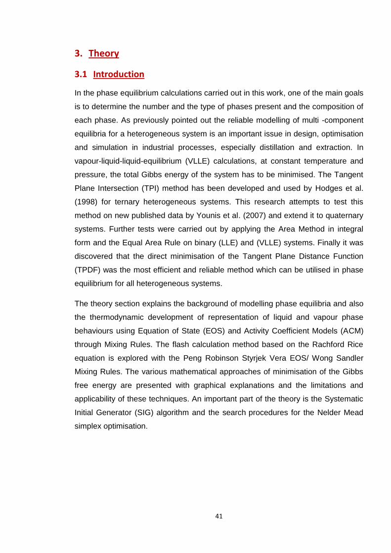
41
3. Theory
3.1 Introduction
In the phase equilibrium calculations carried out in this work, one of the main goals
is to determine the number and the type of phases present and the composition of
each phase. As previously pointed out the reliable modelling of multi -component
equilibria for a heterogeneous system is an important issue in design, optimisation
and simulation in industrial processes, especially distillation and extraction. In
vapour-liquid-liquid-equilibrium (VLLE) calculations, at constant temperature and
pressure, the total Gibbs energy of the system has to be minimised. The Tangent
Plane Intersection (TPI) method has been developed and used by Hodges et al.
(1998) for ternary heterogeneous systems. This research attempts to test this
method on new published data by Younis et al. (2007) and extend it to quaternary
systems. Further tests were carried out by applying the Area Method in integral
form and the Equal Area Rule on binary (LLE) and (VLLE) systems. Finally it was
discovered that the direct minimisation of the Tangent Plane Distance Function
(TPDF) was the most efficient and reliable method which can be utilised in phase
equilibrium for all heterogeneous systems.
The theory section explains the background of modelling phase equilibria and also
the thermodynamic development of representation of liquid and vapour phase
behaviours using Equation of State (EOS) and Activity Coefficient Models (ACM)
through Mixing Rules. The flash calculation method based on the Rachford Rice
equation is explored with the Peng Robinson Styrjek Vera EOS/ Wong Sandler
Mixing Rules. The various mathematical approaches of minimisation of the Gibbs
free energy are presented with graphical explanations and the limitations and
applicability of these techniques. An important part of the theory is the Systematic
Initial Generator (SIG) algorithm and the search procedures for the Nelder Mead
simplex optimisation.
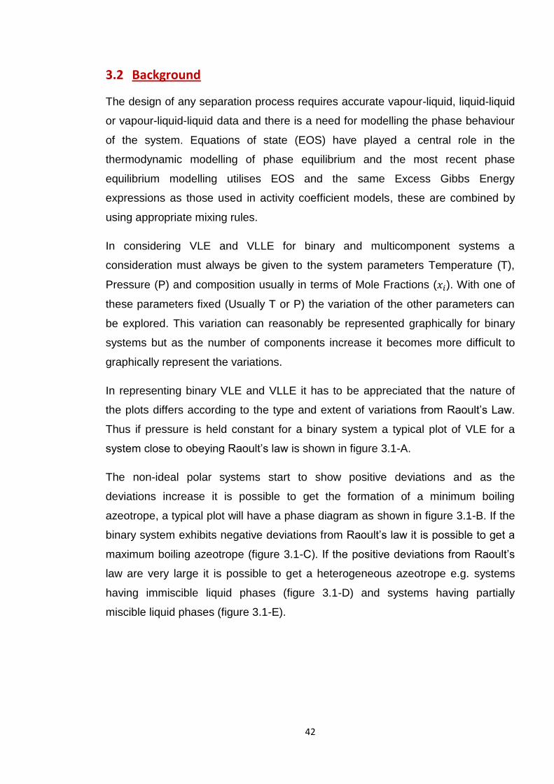
42
3.2 Background
The design of any separation process requires accurate vapour-liquid, liquid-liquid
or vapour-liquid-liquid data and there is a need for modelling the phase behaviour
of the system. Equations of state (EOS) have played a central role in the
thermodynamic modelling of phase equilibrium and the most recent phase
equilibrium modelling utilises EOS and the same Excess Gibbs Energy
expressions as those used in activity coefficient models, these are combined by
using appropriate mixing rules.
In considering VLE and VLLE for binary and multicomponent systems a
consideration must always be given to the system parameters Temperature (T),
Pressure (P) and composition usually in terms of Mole Fractions (𝑥𝑖). With one of
these parameters fixed (Usually T or P) the variation of the other parameters can
be explored. This variation can reasonably be represented graphically for binary
systems but as the number of components increase it becomes more difficult to
graphically represent the variations.
In representing binary VLE and VLLE it has to be appreciated that the nature of
the plots differs according to the type and extent of variations from Raoult’s Law.
Thus if pressure is held constant for a binary system a typical plot of VLE for a
system close to obeying Raoult’s law is shown in figure 3.1-A.
The non-ideal polar systems start to show positive deviations and as the
deviations increase it is possible to get the formation of a minimum boiling
azeotrope, a typical plot will have a phase diagram as shown in figure 3.1-B. If the
binary system exhibits negative deviations from Raoult’s law it is possible to get a
maximum boiling azeotrope (figure 3.1-C). If the positive deviations from Raoult’s
law are very large it is possible to get a heterogeneous azeotrope e.g. systems
having immiscible liquid phases (figure 3.1-D) and systems having partially
miscible liquid phases (figure 3.1-E).
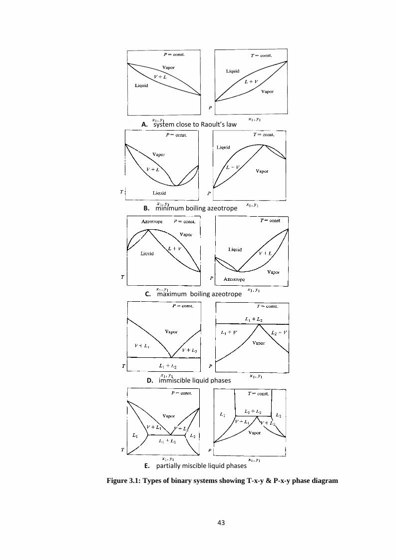
43
Figure 3.1: Types of binary systems showing T-x-y & P-x-y phase diagram
A. system close to Raoult’s law
B. minimum boiling azeotrope
C. maximum boiling azeotrope
D. immiscible liquid phases
E. partially miscible liquid phases

44
Typically a three component (ternary) system, showing deviations from Raoult’s
law can be represented on triangular diagrams. These diagrams are usually
composition diagrams where the liquid and vapour phase compositions can be
represented. This is graphically illustrated by reference to the paper of Younis et
al. (2007).
If it is necessary to also illustrate for example a phase diagram where pressure is
constant and temperature varies then it is usually necessary to use a 3D diagram.
Figure 3.2: T-x-y spatial representation of the VLLE data for a ternary system; (b)
Projection of the VLLE region
This diagram represents the liquid and vapour for a ternary system. The region
below Z represents a typical liquid-liquid phase region at temperatures below the
saturation azeotropic temperature. Point Z represents the binary heterogeneous
azeotrope at the appropriate temperature and pressure composition within the
ternary system; as can be seen from the companioning ternary composition
diagram (b) the heterogeneous azeotrope occurs when the composition of
component B is zero. The line ZR represents vapour phase composition and
corresponding liquid phase compositions can be found using appropriate tie lines
such as CD.
45
For such a ternary system Gibbs phase rule could be applied and writing the rule
for a non-reactive system gives:
𝐹 = 𝐶 − 𝜋 + 2 (3.1)
where 𝐹 is degree of freedom, 𝐶 is number of components and 𝜋 is number of
phases.
For the ternary system described the degree of freedom is 2, thus for a given
conditions there are 2 degrees of freedom appropriately for this system and these
would be designated as temperature and pressure. Gibbs phase rule has been
used throughout this work.
Phase equilibrium calculations are classified into two main categories; flash
calculation and the Gibbs energy minimization (Eubank 1992). The first method is
used in solving the material balance equations and the equality of chemical
potentials. The weakness in this method is the failure to predict the correct number
of phases. The second method utilises global optimisation techniques for the
accurate and reliable prediction of phase Equilibria. (Stadtherr et al., 2007).
Since van der Waals produced the first viable cubic equation of State (EOS) in
1873. Many equations of state have been developed by researchers over the
intervening years e.g. Redlich-Kwong, Soave- Redlich-Kwong (SRK), Peng-
Robinson (PR) and Patel & Teja (Kontogeoris & Gani, 2004; Sandler 1994).
The Stryjek-Vera modification of Peng-Robinson EOS and Wong Sandler mixing
rule (WSMR) incorporated with modified UNiversal QUAsi Chemical (UNIQUAC)
activity model is used in this research.
In phase Equilibria calculations several mixing rules have been developed to
extend the applicability of the EOS in predicting VLE & VLLE for highly non-ideal
polar systems. Wong and Sandler (1992) suggested mixing rules utilising excess
Gibbs free energy models in which they combined the attractive term 𝒂 and co-
volume 𝑏 through a mathematical relationship.
A fundamental concept in phase equilibria calculations is minimising the total
Gibbs energy of the system. This method as outlined by Michelsen (1982 a, b) is
done in two stages: phase stability (using tangent plane analysis) and phase split.
46
The major failure with his method is that a good initial phase estimate is required
and there is no guarantee that all the stationary points of the tangent plane
distance have been found. To overcome this problem the area method was
adopted by Eubank et al. (1992) for binary systems and although this produces
more reliable predictions than the Michelsen method it is a computationally time
consuming process. Hodges et al. (1996) suggested that it was mathematically
possible to extend the area method to ternary systems (volume method). The
volume method was tested and ultimately failed due to the incorrect bounding of
the reduced Gibbs energy of the mixing surface (∅) by the 3-phase prism during
the integration of the surface. Although the results for some binary systems agree
with the experimental data some were poor, particularly the systems with very
small mutual solubility.
Hodges et al.(1998) successfully used an alternative approach to the integral area
method namely the tangent plane intersection method (TPI) applied to a range of
binary and ternary 2 and 3-phase mixtures. They announced that the TPI method
could be extended to quaternary 3-phase systems. This work is continuing to
develop the TPI method for multi-phase multi-component heterogeneous systems.
In studying the phase equilibrium of a mixture at constant temperature and
pressure the most important criteria is to predict the composition of each
component in different phases and also the number of phases. It is crucial to know
the behaviour of the system at the design stage of the separation process.
As stated previously the thermodynamic calculation for phase equilibrium is
classified into two main categories; flash calculation and the Gibbs energy
minimization .The first method solves a number of equations relating to material
balance and the equality of chemical potentials; this is a classical solution which is
unable to predict the correct number of phases. The second method is based on
the Michelson tangent plane stability analysis (Michelsen, 1982a, b) this does not
guarantee the global equilibrium solution due to a failure in finding the stationary
points of the tangent plane distance. An alternative for phase stability analysis is
the use of an interval-Newton approach (Schnepper and Stadtherr, 1996) which is
defined as an equation solving method. Stadtherr and his colleagues concluded
that in the computation of phase equilibrium there is a challenging problem and

47
although many solutions have been proposed these methods may still fail to solve
the problem correctly in some cases. (Stadtherr et al., 2007)
In phase equilibrium prediction the requirement is to model the Gibbs energy of
the system according to temperature, pressure and composition of the system. In
general there are two types to represent vapour and liquid; the Excess Gibbs
energy model (activity coefficient models) and Equation of State (EOS) models.
3.3 Thermodynamic of Phase Equilibrium
The basic requirement for phases to be at equilibrium for pure component or multi
component systems is that the state variables (temperature, pressure, chemical
potential) must be equal for all the phases. Equilibrium between phases (𝛼, 𝛽, 𝛾 … )
in a multi-component system means that:
𝑇𝛼 = 𝑇𝛽 = 𝑇𝛾 … (3.2)
𝑃𝛼 = 𝑃𝛽 = 𝑃𝛾 … (3.3)
𝜇𝑖𝛼 = 𝜇𝑖
𝛽= 𝜇𝑖
𝛾… (3.4)
The chemical potential 𝜇 can be expressed in term of fugacities:
𝑓𝑖𝛼 = 𝑓𝑖
𝛽= 𝑓𝑖
𝛾… (𝑖 = 1,2,3, … 𝑛) (3.5)
If the case is vapour-liquid equilibrium:
𝑓𝑖𝐺 = 𝑓𝑖
𝐿 (3.6)
The vapour phase fugacity can be expressed:
𝑓𝑖𝐺 = 𝑦𝑖𝜙𝑖𝑃 (3.7)
𝜙𝑖 is the fugacity coefficient which approaches unity for low pressure.
𝜙𝑖 = 𝑒𝑥𝑝 (1
𝑅𝑇∫ (𝑉𝑖
𝐺 −𝑅𝑇
𝑃) 𝑑𝑃
𝑃
0) (3.8)
Using Peng Robinson 𝜙𝑖 can be written in the term:
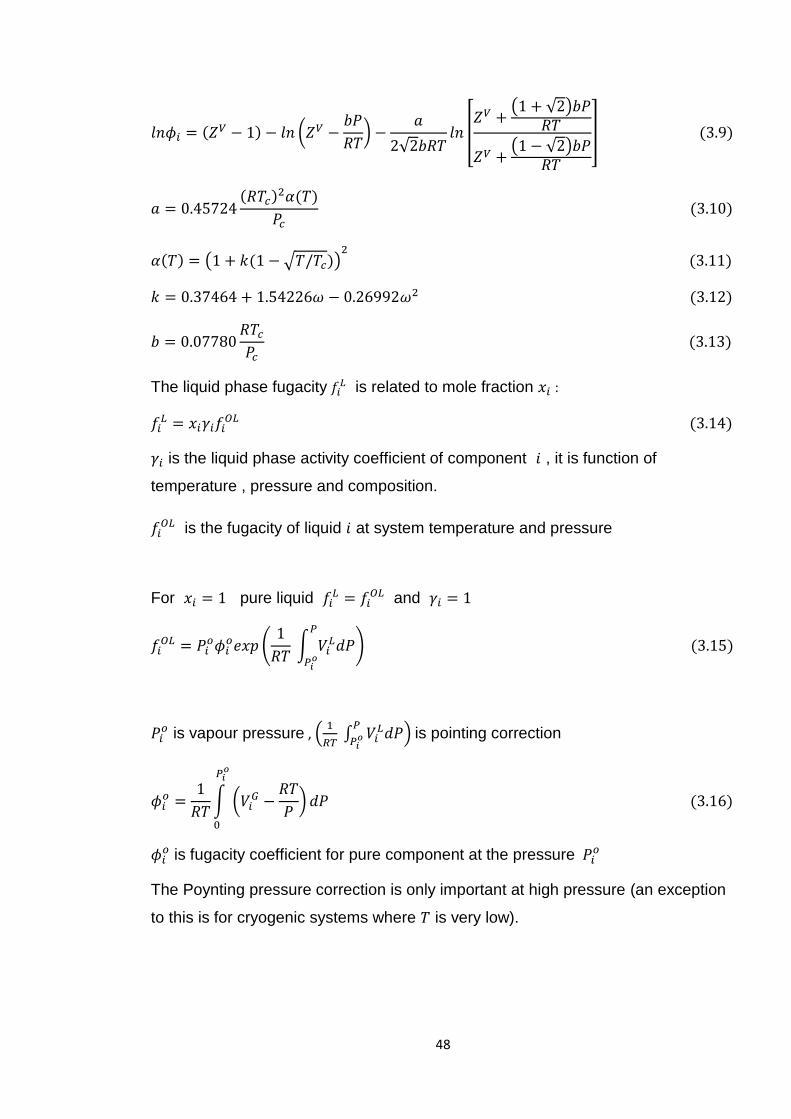
48
𝑙𝑛𝜙𝑖 = (𝑍𝑉 − 1) − 𝑙𝑛 (𝑍𝑉 −𝑏𝑃
𝑅𝑇) −
𝑎
2√2𝑏𝑅𝑇𝑙𝑛 [
𝑍𝑉 +(1 + √2)𝑏𝑃
𝑅𝑇
𝑍𝑉 +(1 − √2)𝑏𝑃
𝑅𝑇
] (3.9)
𝑎 = 0.45724(𝑅𝑇𝑐)2𝛼(𝑇)
𝑃𝑐 (3.10)
𝛼(𝑇) = (1 + 𝑘(1 − √𝑇/𝑇𝑐))2
(3.11)
𝑘 = 0.37464 + 1.54226𝜔 − 0.26992𝜔2 (3.12)
𝑏 = 0.07780𝑅𝑇𝑐
𝑃𝑐 (3.13)
The liquid phase fugacity 𝑓𝑖𝐿 is related to mole fraction 𝑥𝑖 :
𝑓𝑖𝐿 = 𝑥𝑖𝛾𝑖𝑓𝑖
𝑂𝐿 (3.14)
𝛾𝑖 is the liquid phase activity coefficient of component 𝑖 , it is function of
temperature , pressure and composition.
𝑓𝑖𝑂𝐿 is the fugacity of liquid 𝑖 at system temperature and pressure
For 𝑥𝑖 = 1 pure liquid 𝑓𝑖𝐿 = 𝑓𝑖
𝑂𝐿 and 𝛾𝑖 = 1
𝑓𝑖𝑂𝐿 = 𝑃𝑖
𝑜𝜙𝑖𝑜𝑒𝑥𝑝 (
1
𝑅𝑇 ∫ 𝑉𝑖
𝐿𝑑𝑃𝑃
𝑃𝑖𝑜
) (3.15)
𝑃𝑖𝑜 is vapour pressure , (
1
𝑅𝑇 ∫ 𝑉𝑖
𝐿𝑑𝑃𝑃
𝑃𝑖𝑜 ) is pointing correction
𝜙𝑖𝑜 =
1
𝑅𝑇∫ (𝑉𝑖
𝐺 −𝑅𝑇
𝑃) 𝑑𝑃
𝑃𝑖𝑜
0
(3.16)
𝜙𝑖𝑜 is fugacity coefficient for pure component at the pressure 𝑃𝑖
𝑜
The Poynting pressure correction is only important at high pressure (an exception
to this is for cryogenic systems where 𝑇 is very low).

49
3.4 Equations of State
Since van der Waals found the thermodynamic relationship between 𝑇, 𝑉 and 𝑃 for
a system many EOS have been developed. Most of these equations have two
specific parameters (𝑎, 𝑏) , 𝑎 is related to molecular energy and the energetic
interaction 𝑏 called co-volume, to the molecular volume. The pure fluid parameters
are estimated from the critical properties and acentric factor. In modelling phase
equilibrium for mixtures these parameters are extended to mixtures by applying
the appropriate mixing rules. Historically the most used mixing rules have been
van der Waals one fluid mixing rules 1VDWMR and 2VDWMR (Kontogeorgis et
al., 2004). In a later section there is an explanation of the mixing rules. The
advantage of EOS is that they can be used over a wide range of temperatures and
pressures. The modified PR EOS by Stryjek-Vera is shown below (equation 3.16):
𝑃 =𝑅𝑇
𝑣 − 𝑏−
𝑎
𝑣2 + 2𝑏𝑣 − 𝑏2 (3.17)
In the phase equilibrium criteria the starting point for VLLE calculation is the
thermodynamic requirement that the temperature (𝑇), pressure (𝑃), partial molar
Gibbs energy and fugacity of each species be same in all phases:
�̅�𝑖𝐼(𝑥𝑖
𝐼 , 𝑇, 𝑃) = �̅�𝑖𝐼𝐼(𝑥𝑖
𝐼𝐼 , 𝑇, 𝑃) = �̅�𝑖𝐼𝐼𝐼(𝑥𝑖
𝐼𝐼𝐼, 𝑇, 𝑃) = ⋯
The equality of fugacity for VLE:
𝑓�̅�𝐿(𝑥𝑖, 𝑇, 𝑃) = 𝑓�̅�
𝑉(𝑦𝑖, 𝑇, 𝑃) for 𝑖 = 1,2,3, … 𝑛
The Peng- Robinson EOS to calculate the fugacity of a component in a liquid
mixture is:
ln (𝑓𝑖𝐿(𝑇, 𝑃, 𝑥𝑖)
𝑥𝑖𝑃=
𝐵𝑖
𝐵(𝑍𝐿 − 1) − 𝑙𝑛(𝑍𝐿 − 𝐵)
−𝐴
2√2𝐵[2 ∑ 𝑥𝑖𝐴𝑖𝑗
𝑛𝑖
𝐴−
𝐵𝑖
𝐵] 𝑙𝑛 [
𝑍𝐿 + (√2 + 1)𝐵
𝑍𝐿 − (√2 + 1)𝐵] (3.18)
where 𝐴 =𝑎𝑃
(𝑅𝑇)2 , 𝐵 =𝑏𝑃
𝑅𝑇 the subscript 𝐿 refers to liquid phase (Sandler 1989).
In applying the above equation to vapour phase subscript 𝐿 must be changed to 𝑉.

50
3.5 Activity Coefficients
Liquid phase models were developed to determine the departure of a real mixture
from the ideal behaviour of low pressure VLE and LLE systems. Renon and
Prausntiz (1968) proposed the Non Random Two Liquid (NRTL) equation and later
it was extended for multicomponent systems. These models are capable of
representing adequately the excess Gibbs energy for a mixture through calculation
of the activity coefficient γ𝑖 of each component.
There are two different methods for the description of VLE. The Gamma-Phi (γ −
𝜙) method in which the liquid phase is represented with an activity coefficient
model e.g UNIQUAC and EOS used for vapour phase. Phi-Phi (𝜙 − 𝜙) is the
second method in which EOS represents both phases. The Phi-Phi method is
used in this work and both phases have been represented by Peng Robinson
Stryjek Vera (PRSV)(1986) combined with Wong Sandler Mixing Rules (WSMR)
through the UNIQUAC model which represents the excess Gibbs energy part in
the mixing rule.
The modified UNIQUAC equation for excess Gibbs energy gE consists of two
parts: combinatorial and residual. The combinatorial part represents the size and
shape of the molecules and the residual part represents interaction energies
between molecules:
gE(𝑐𝑜𝑚𝑏𝑖𝑛𝑎𝑡𝑜𝑟𝑖𝑎𝑙)
𝑅𝑇= ∑ 𝑥𝑖𝑙𝑛
𝜑𝑖
𝑥𝑖+
𝑧
2𝑖
∑ 𝑞𝑖
𝑖
𝑥𝑖𝑙𝑛𝜃𝑖
𝜑𝑖 (3.19)
gE(𝑟𝑒𝑠𝑖𝑑𝑢𝑎𝑙)
𝑅𝑇= − ∑ �̅�𝑖
𝑖
𝑥𝑖𝑙𝑛 (∑ �̅�𝑖𝜏𝑗𝑖
𝑖
) (3.20)
Where segment fraction for 𝜑 and �̅� are given by
𝜑𝑖 =𝑟𝑖𝑥𝑖
∑ 𝑟𝑗𝑥𝑗𝑗 𝜃𝑖 =
𝑞𝑖𝑥𝑖
∑ 𝑞𝑗𝑥𝑗𝑗 �̅�𝑖 =
�̅�𝑖𝑥𝑖
∑ �̅�𝑗𝑥𝑗𝑗
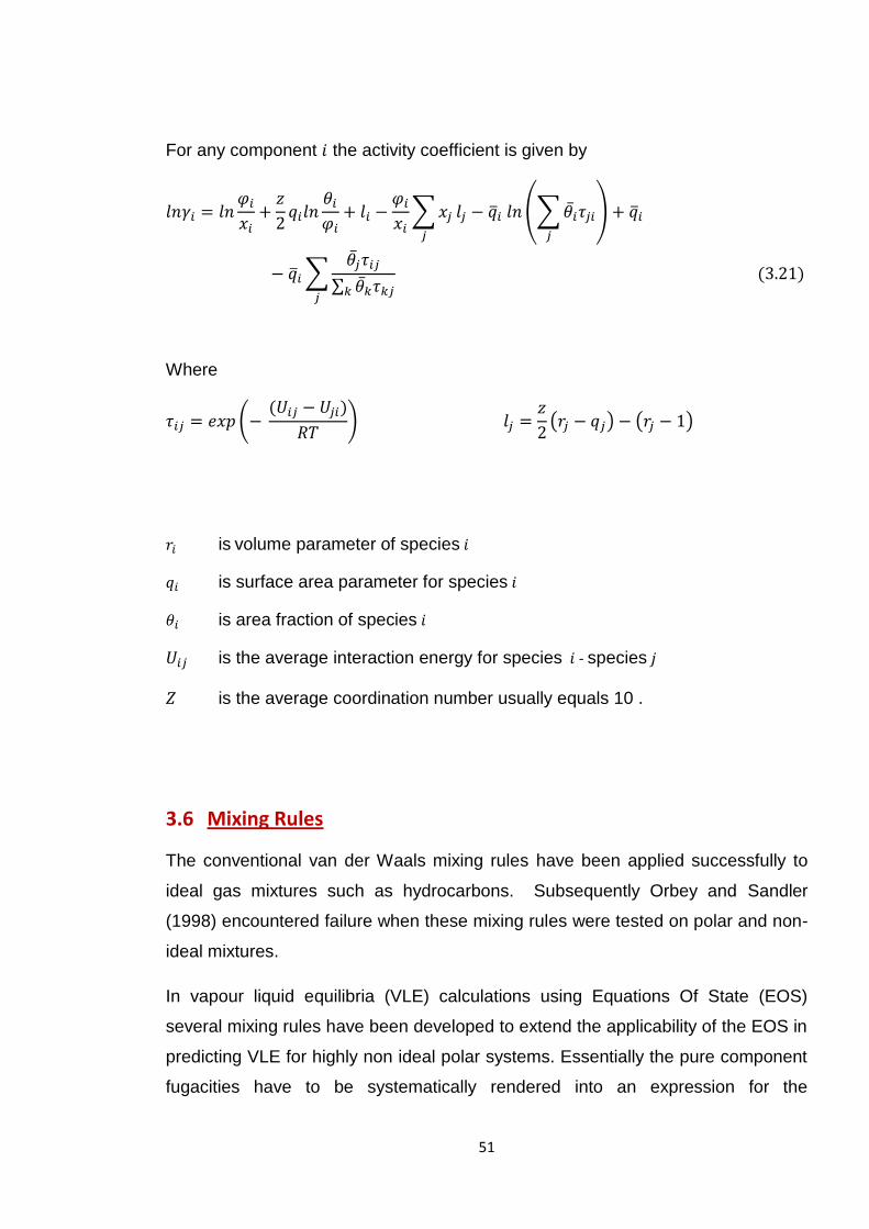
51
For any component 𝑖 the activity coefficient is given by
𝑙𝑛𝛾𝑖 = 𝑙𝑛𝜑𝑖
𝑥𝑖+
𝑧
2𝑞𝑖𝑙𝑛
𝜃𝑖
𝜑𝑖+ 𝑙𝑖 −
𝜑𝑖
𝑥𝑖∑ 𝑥𝑗
𝑗
𝑙𝑗 − �̅�𝑖 𝑙𝑛 (∑ �̅�𝑖𝜏𝑗𝑖
𝑗
) + �̅�𝑖
− �̅�𝑖 ∑�̅�𝑗𝜏𝑖𝑗
∑ �̅�𝑘𝜏𝑘𝑗𝑘𝑗
(3.21)
Where
𝜏𝑖𝑗 = 𝑒𝑥𝑝 (− (𝑈𝑖𝑗 − 𝑈𝑗𝑖)
𝑅𝑇) 𝑙𝑗 =
𝑧
2(𝑟𝑗 − 𝑞𝑗) − (𝑟𝑗 − 1)
𝑟𝑖 is volume parameter of species 𝑖
𝑞𝑖 is surface area parameter for species 𝑖
𝜃𝑖 is area fraction of species 𝑖
𝑈𝑖𝑗 is the average interaction energy for species 𝑖 - species 𝑗
𝑍 is the average coordination number usually equals 10 .
3.6 Mixing Rules
The conventional van der Waals mixing rules have been applied successfully to
ideal gas mixtures such as hydrocarbons. Subsequently Orbey and Sandler
(1998) encountered failure when these mixing rules were tested on polar and non-
ideal mixtures.
In vapour liquid equilibria (VLE) calculations using Equations Of State (EOS)
several mixing rules have been developed to extend the applicability of the EOS in
predicting VLE for highly non ideal polar systems. Essentially the pure component
fugacities have to be systematically rendered into an expression for the
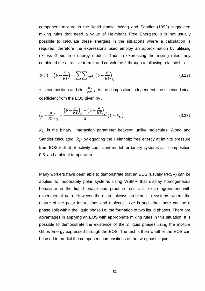
52
component mixture in the liquid phase. Wong and Sandler (1992) suggested
mixing rules that need a value of Helmholtz Free Energies. It is not usually
possible to calculate these energies in the situations where a calculation is
required; therefore the expressions used employ an approximation by utilising
excess Gibbs free energy models. Thus in expressing the mixing rules they
combined the attractive term 𝑎 and co-volume 𝑏 through a following relationship:
𝐵(𝑇) = (𝑏 −𝑎
𝑅𝑇) = ∑ ∑ 𝑥𝑖𝑥𝑗 (𝑏 −
𝑎
𝑅𝑇)
𝑖𝑗 (3.22)
𝑥 is composition and (𝑏 −𝑎
𝑅𝑇)𝑖𝑗 is the composition independent cross second virial
coefficient from the EOS given by :
(𝑏 −𝑎
𝑅𝑇)
𝑖𝑗=
(𝑏 −𝑎
𝑅𝑇)𝑖𝑖
+ (𝑏 −𝑎
𝑅𝑇)𝑗𝑗
2(1 − 𝑘𝑖𝑗) (3.23)
𝑘𝑖𝑗 is the binary interaction parameter between unlike molecules. Wong and
Sandler calculated 𝑘𝑖𝑗 by equating the Helmholtz free energy at infinite pressure
from EOS to that of activity coefficient model for binary systems at composition
0.5 and ambient temperature .
Many workers have been able to demonstrate that an EOS (usually PRSV) can be
applied to moderately polar systems using WSMR that display homogeneous
behaviour in the liquid phase and produce results in close agreement with
experimental data. However there are always problems in systems where the
nature of the polar interactions and molecule size is such that there can be a
phase split within the liquid phase i.e. the formation of two liquid phases. There are
advantages in applying an EOS with appropriate mixing rules in this situation. It is
possible to demonstrate the existence of the 2 liquid phases using the mixture
Gibbs Energy expressed through the EOS. The test is then whether the EOS can
be used to predict the component compositions of the two-phase liquid.

53
In this work, systems were chosen to check certain predictions that had already
been made and then produce a working algorithm that could be tested by applying
it to other experimentally measured systems. Thus a range of systems were
chosen that would test the EOS with mixing rules within homogeneous and
heterogeneous regions.
Six binary VLE mixtures were modelled using PRSV combined with UNIQUAC
activity coefficient. The systems selected are homogenous from slightly non-ideal
to heterogeneous highly non-ideal polar systems: (methanol-water, ethanol-water,
1-propanol-water, water-n butanol, MEK-water and water-hexanol).
The section below sets out the specific form of the PRSV EOS used with the
WSMR. These equations have been used to produce a working model for
homogeneous and heterogeneous vapour liquid equilibria initially for binary
systems.
3.7 Thermodynamic model description
The equation of state used in this work is Peng Robinson EOS modified by Stryjek
Vera (1986a) combined with Wong Sandler Mixing Rules which utilises modified
UNIQUAC as an activity coefficient model in the calculation of excess Gibbs
energy (1992). The equations needed to estimate the pure component parameters
𝑎𝑖 and 𝑏𝑖 are:
𝑎𝑖 =0.457235𝑅2 𝑇𝑐𝑖
2𝛼𝑖
𝑃𝑐𝑖
(3.24)
𝑏𝑖 =0.077796 𝑅 𝑇𝑐𝑖
𝑃𝑐𝑖
(3.25)
where:

54
𝛼𝑖 = [1 + 𝐾𝑖 (1 − √𝑇𝑅𝑖)]
2
(3.26)
𝐾𝑖 = 𝐾0𝑖+ 𝐾1𝑖
(1 + √𝑇𝑅𝑖)(0.7 − 𝑇𝑅𝑖
) (3.27)
𝐾0𝑖= 0.378893 + 1.4897153 𝜔𝑖 − 0.17131848 𝜔𝑖
2 + 0.0196554 𝜔𝑖2 (3.28)
𝑇𝑅𝑖=
𝑇
𝑇𝑐𝑖
(3.29)
Wong and Sandler (1992) demonstrated in their work the applicability of their
Mixing Rules which they developed by testing experimental vapour – liquid, vapour
– liquid- liquid and liquid – liquid equilibrium data for several binary systems
(cyclohexane- water , propane – methanol and benzene-ethanol) and ternary
systems ( Carbon dioxide –propane – methanol) at low and high pressure. The
systems are in a range of ideal to highly non ideal mixtures. They have shown that
their mixing rules can be used for a wide variety of mixtures and phase behaviour
and also for the systems that could not be described with EOS. The modified
PRSV EOS is:
𝑃 =𝑅𝑇
(𝑣 − 𝑏)−
𝑎
(𝑣2 + 2𝑏𝑣 − 𝑏2) (3.30)
where:
𝐴 =𝑎𝑃
(𝑅𝑇)2 𝐵 =
𝑏𝑃
𝑅𝑇
the relationship between the mixture parameters 𝑎 and 𝑏 is defined as:
𝑎 = 𝑅𝑇𝑄𝐷
(1 − 𝐷) 𝑏 =
𝑄
(1 − 𝐷)
with
𝑄 = ∑ ∑ 𝑥𝑖
𝑗𝑖
𝑥𝑗 (𝑏 −𝑎
𝑅𝑇)
𝑖𝑗 (3.31)
𝐷 = ∑ 𝑥𝑖
𝑖
(𝑎𝑖
𝑏𝑖𝑅𝑇) + (
�̅�𝑒𝑥
𝐶𝑅𝑇) (3.32)
then the term (𝑏 −𝑎
𝑅𝑇)
𝑖𝑗 is determined with the following combining rules:

55
(𝑏 −𝑎
𝑅𝑇)
𝑖𝑗=
1
2[(𝑏𝑖 −
𝑎𝑖
𝑅𝑇) + (𝑏𝑗 −
𝑎𝑗
𝑅𝑇)] (1 − 𝑘𝑖𝑗) (3.33)
PRSV EOS with WS mixing rules equation in the form of fugacity coefficient is:
𝑙𝑛𝜙𝑖 = −𝑙𝑛 [𝑃(𝑣 − 𝑏)
𝑅𝑇] +
1
𝑏(
𝜕𝑛𝑏
𝜕𝑛𝑖) (
𝑃𝑣
𝑅𝑇− 1)
+1
2√2(
𝑎
𝑏𝑅𝑇) [
1
𝑎(
1
𝑛
𝜕𝑛2𝑎
𝜕𝑛𝑖) −
1
𝑏(
𝜕𝑛𝑏
𝜕𝑛𝑖)] 𝑙𝑛 [
𝑣 + 𝑏(1 − √2)
𝑣 + 𝑏(1 + √2)] (3.34)
(𝜕𝑛𝑏
𝜕𝑛𝑖) =
1
(1 − 𝐷)(
1
𝑛
𝜕𝑛2𝑄
𝜕𝑛𝑖) −
𝑄
(1 − 𝐷)2(1 −
𝜕𝐷
𝜕𝑛𝑖) (3.35)
1
𝑅𝑇(
1
𝑛
𝜕𝑛2𝑎
𝜕𝑛𝑖) = 𝐷
𝜕𝑏
𝜕𝑛𝑖+ 𝑏
𝜕𝐷
𝜕𝑛𝑖 (3.36)
(1
𝑛
𝜕𝑛2𝑄
𝜕𝑛𝑖) = 2 ∑ 𝑥𝑗
𝑗
(𝑏 −𝑎
𝑅𝑇)
𝑖𝑗 (3.37)
and
𝜕𝐷
𝜕𝑛𝑖=
𝑎𝑖
𝑏𝑖𝑅𝑇+
𝑙𝑛𝛾𝑖∞
𝐶 (3.38)
with
𝑙𝑛𝛾𝑖∞ =1
𝑅𝑇
𝜕𝑛 𝐴∞𝐸
𝜕𝑛𝑖 (3.39)
𝐶 is a constant dependent on the equation of state being used and for PRSV EOS
is defined as:
𝐶 =1
√2𝑙𝑛(√2 − 1) (3.40)
56
Equation (3.34) has been used through this work to calculate the component
fugacity coefficients in the mixture in both liquid and vapour phases. The PRSV
EOS can be written in this form:
𝑍3 + 𝛼𝑍2 + 𝛽𝑍 + 𝛾 = 0 (3.41)
The parameters for the above equation are:
𝛼 = −1 + 𝐵
𝛽 = 𝐴 − 3𝐵2 − 2𝐵
𝛾 = −𝐴𝐵 + 𝐵2 + 𝐵3
𝐴 and 𝐵 are defined earlier in this section .
The solution for the cubic equation of state (equation 3.40) for compressibility
factor produces three roots. The large value of the root is used for vapour phase
and the small value is used for liquid phase fugacity calculation. (Sandler, 2006)
The minimization function used by Orbey (Orbey et al., 1993) is based on equality
for excess Gibbs energy from the Activity Coefficient Model UNIQUAC and PRSV
EOS to estimate binary interaction parameters. This estimation was based on the
assumption that the system is at ambient condition and the composition is 0.5.
(𝐺𝑒𝑥
𝑅𝑇)
𝐸𝑂𝑆
= (𝐺𝑒𝑥
𝑅𝑇)
𝐴𝑐
(3.42)
This work relies on the experimental data for the systems investigated to obtain
the binary interaction parameters values for PRSV EOS.
3.8 Estimation of parameters
In thermodynamic phase equilibrium modelling, an important requirement is the
estimation of parameters by determining the value of model parameters that
provide the ‘best fit’ to the set of the experimental data. The VLE, LLE and VLLE
data reduction is generally based on least squares or maximum likelihood
approach. The most popular approach according to literature is the least square
objective function (Lopez et al., 2006). In the VLE data correlation for isothermal
and isobaric condition the objective functions used are:
57
𝐹 = ∑ ∑ [𝑦𝑖𝑗
𝑒𝑥𝑝 − 𝑦𝑖𝑗𝑐𝑎𝑙
𝜎𝑦]
2𝑛𝑐
𝑖
𝑛
𝑗
+ ∑ [𝑃𝑗
𝑒𝑥𝑝 − 𝑃𝑗𝑐𝑎𝑙
𝜎𝑃]
2
+
𝑛
𝑗
∑ [𝑇𝑗
𝑒𝑥𝑝 − 𝑇𝑗𝑐𝑎𝑙
𝜎𝑇]
2𝑛
𝑗
(3.43)
Where 𝑛 , 𝑛𝑐 are the number of data points and the number of components in the
mixture respectively, and 𝜎𝑦 , 𝜎𝑃 , 𝜎𝑇 are the standard deviation in vapour mole
fraction, pressure and temperature respectively. Equation (3.43) is minimised
using the Nelder-Mead simplex to obtain the UNIQUAC energy parameters
𝜏𝑖𝑗 and 𝑘𝑖𝑗 the binary interaction parameter used in PRSV EOS.
𝐹 = ∑ ∑ [𝑦𝑖𝑗
𝑒𝑥𝑝 − 𝑦𝑖𝑗𝑐𝑎𝑙
𝑦𝑖𝑗𝑒𝑥𝑝 ]
2𝑛𝑐
𝑖
+ [𝑃𝑖𝑗
𝑒𝑥𝑝 − 𝑃𝑖𝑗𝑐𝑎𝑙
𝑃𝑖𝑗𝑒𝑥𝑝 ]
2
𝑛
𝑗
+ [𝑇𝑖𝑗
𝑒𝑥𝑝 − 𝑇𝑖𝑗𝑐𝑎𝑙
𝑇𝑖𝑗𝑒𝑥𝑝 ]
2
(3.44)
In modelling LLE the objective function used can be written as:
𝐹 = ∑ ∑ |𝑥𝑖𝑗𝑜𝑟𝑔
𝑒𝑥𝑝 − 𝑥𝑖𝑗𝑜𝑟𝑔
𝑐𝑎𝑙
𝑥𝑖𝑗𝑜𝑟𝑔
𝑒𝑥𝑝 |
𝑛𝑐
𝑖
+ |𝑥𝑖𝑗𝑎𝑞
𝑒𝑥𝑝 − 𝑥𝑖𝑗𝑎𝑞
𝑐𝑎𝑙
𝑥𝑖𝑗𝑎𝑞
𝑒𝑥𝑝 |
𝑛
𝑗
(3.45)
The objective function used in VLLE calculation is based on minimisation of the
average absolute deviation for composition in organic, aqueous and vapour
phases and also pressure and temperature for each data point of the calculation.
𝐹 = ∑ ∑ |𝑥𝑖𝑗𝑜𝑟𝑔
𝑒𝑥𝑝− 𝑥𝑖𝑗𝑜𝑟𝑔
𝑐𝑎𝑙
𝑥𝑖𝑗𝑜𝑟𝑔
𝑒𝑥𝑝 |
𝑛𝑐
𝑖
+ |𝑥𝑖𝑗𝑎𝑞
𝑒𝑥𝑝− 𝑥𝑖𝑗𝑎𝑞
𝑐𝑎𝑙
𝑥𝑖𝑗𝑎𝑞
𝑒𝑥𝑝 |
𝑛
𝑗
+ |𝑦𝑖𝑗
𝑒𝑥𝑝− 𝑦𝑖𝑗𝑜𝑟𝑔
𝑐𝑎𝑙
𝑦𝑖𝑗𝑒𝑥𝑝 | + |
𝑦𝑖𝑗𝑒𝑥𝑝
− 𝑦𝑖𝑗𝑎𝑞
𝑐𝑎𝑙
𝑦𝑖𝑗𝑒𝑥𝑝 | (3.46)
𝐹 = ∑ ∑ |𝑃𝑖𝑗
𝑒𝑥𝑝− 𝑃𝑖𝑗
𝑐𝑎𝑙
𝑃𝑖𝑗𝑒𝑥𝑝 |
𝑛𝑐
𝑖
|𝑇𝑖𝑗
𝑒𝑥𝑝− 𝑇𝑖𝑗
𝑐𝑎𝑙
𝑇𝑖𝑗𝑒𝑥𝑝 |
𝑛
𝑗
(3.47)
In modelling VLLE flash calculation, equation (3.46) reduces to three parts and
can be expressed as:
𝐹 = ∑ ∑ |𝑥𝑖𝑗𝑜𝑟𝑔
𝑒𝑥𝑝− 𝑥𝑖𝑗𝑜𝑟𝑔
𝑐𝑎𝑙
𝑥𝑖𝑗𝑜𝑟𝑔
𝑒𝑥𝑝 |
𝑛𝑐
𝑖
+ |𝑥𝑖𝑗𝑎𝑞
𝑒𝑥𝑝− 𝑥𝑖𝑗𝑎𝑞
𝑐𝑎𝑙
𝑥𝑖𝑗𝑎𝑞
𝑒𝑥𝑝 |
𝑛
𝑗
+ |𝑦𝑖𝑗
𝑒𝑥𝑝 − 𝑦𝑖𝑗𝑐𝑎𝑙
𝑦𝑖𝑗𝑒𝑥𝑝 | (3.48)

58
were 𝑛 is the number of data points and 𝑛𝑐 is the number of components in the
mixture.
3.9 VLLE three phase Flash calculation
The Modified Peng Robinson equation of state as proposed by Styrjek and Vera
has been used successfully to describe the multiphase multi-component
heterogeneous systems of Younis et al. (2007). In the flash calculation formulation
for VLLE of multi-component the mass balances and summations are:
𝐹 = 𝑉 + 𝐿𝑜𝑟𝑔 + 𝐿𝑎𝑞 (3.49)
𝑧𝑖𝐹 = 𝑦𝑖𝑉 + 𝑥𝑖𝑜𝑟𝑔
𝐿𝑜𝑟𝑔 + 𝑥𝑖𝑎𝑞𝐿𝑎𝑞 ; 𝑖 = 1,2, … , 𝑛𝑐 (3.50)
∑ 𝑥𝑖𝑜𝑟𝑔
𝑛𝑐
𝑖=1
= ∑ 𝑥𝑖𝑎𝑞
𝑛𝑐
𝑖=1
= ∑ 𝑦𝑖
𝑛𝑐
𝑖=1
= 1 (3.51)
The superscripts 𝑎𝑞 and 𝑜𝑟𝑔 refer to aqueous and organic phases respectively.
The iso-activity criterion gives:
𝑦𝑖 = 𝐾𝑖,𝑜𝑟𝑔 𝑥𝑖𝑜𝑟𝑔
𝑖 = 1,2, … , 𝑛𝑐 (3.52𝑎)
𝑦𝑖 = 𝐾𝑖,𝑎𝑞 𝑥𝑖𝑎𝑞 𝑖 = 1,2, … , 𝑛𝑐 (3.52𝑏)
In the above equations (3.52𝑎 &𝑏) the 𝐾𝑖 can be expressed in form of
thermodynamic models, using EOS to estimate the equilibrium constants:
𝐾𝑖,𝑜𝑟𝑔 =𝜙𝑖
𝑜𝑟𝑔
𝜙𝑖𝑣 ; 𝐾𝑖,𝑎𝑞 =
𝜙𝑖𝑎𝑞
𝜙𝑖𝑣 (3.53)
Substituting equation (3.52) into equation (3.50), and rearranging yields:
𝑦𝑖 =𝑧𝑖𝐾𝑖,𝑜𝑟𝑔𝐾𝑖,𝑎𝑞
𝐾𝑖,𝑜𝑟𝑔𝐾𝑖,𝑎𝑞 + 𝜃𝑜𝑟𝑔𝐾𝑖,𝑎𝑞(1 − 𝐾𝑖,𝑜𝑟𝑔) + 𝜃𝑎𝑞𝐾𝑖,𝑜𝑟𝑔(1 − 𝐾𝑖,𝑎𝑞) (3.54)

59
𝑥𝑖𝑜𝑟𝑔
=𝑧𝑖𝐾𝑖,𝑎𝑞
𝐾𝑖,𝑜𝑟𝑔𝐾𝑖,𝑎𝑞 + 𝜃𝑜𝑟𝑔𝐾𝑖,𝑎𝑞(1 − 𝐾𝑖,𝑜𝑟𝑔) + 𝜃𝑎𝑞𝐾𝑖,𝑜𝑟𝑔(1 − 𝐾𝑖,𝑎𝑞) (3.55)
𝑥𝑖𝑎𝑞 =
𝑧𝑖𝐾𝑖,𝑜𝑟𝑔
𝐾𝑖,𝑜𝑟𝑔𝐾𝑖,𝑎𝑞 + 𝜃𝑜𝑟𝑔𝐾𝑖,𝑎𝑞(1 − 𝐾𝑖,𝑜𝑟𝑔) + 𝜃𝑎𝑞𝐾𝑖,𝑜𝑟𝑔(1 − 𝐾𝑖,𝑎𝑞) (3.56)
where 𝑖 = 1,2, … , 𝑛𝑐 , 𝜃𝑜𝑟𝑔 𝑎𝑛𝑑 𝜃𝑎𝑞 are the fractions of molar flow rate of organic
and aqueous liquid phase with respect to the overall feed 𝐹 .
The combination of the equations (3.54, 3.55, and 3.56) can be used to determine
the thermodynamic properties of the three phases. Peng and Robinson
recommended the following equation for VLLE flash calculations:
∑ 𝑥𝑖,𝑜𝑟𝑔 −
𝑛𝑐
𝑖=1
∑ 𝑦𝑖 = 0
𝑛𝑐
𝑖=1
, [∑ 𝑥𝑖,𝑎𝑞
𝑛𝑐
𝑖=1
] − 1 = 0 (3.57)
Equation (3.57) is known as the Rachford Rice equation, it can be solved
simultaneously using any iterative method and the initial values of equilibrium
ratios must be provided to enable the flash equilibrium calculation to proceed
reliably. Peng and Robinson adopted Wilson’s equilibrium ratio correlation to
provide initial values for 𝐾𝑖,𝑜𝑟𝑔 in the following equation:
𝐾𝑖,𝑜𝑟𝑔 =𝑃𝑐𝑖
𝑃𝑒𝑥𝑝 [5.3727(1 + 𝜔𝑖) (1 −
𝑇𝑐𝑖
𝑇)] (3.58𝑎)
Where 𝑃 is total pressure in psia; 𝑇 is system temperature in Fahrenheit; 𝑃𝑐𝑖is
critical pressure of component 𝑖, and 𝑇𝑐𝑖 is critical temperature of component 𝑖 and
𝜔𝑖 is acentric factor of component 𝑖. Peng and Robinson proposed the following
expression to estimate the initial values for 𝐾𝑖,𝑎𝑞 (Mokhatab, 2003):
𝐾𝑖,𝑎𝑞 = 106 [𝑃𝑐𝑖
. 𝑇
𝑃. 𝑇𝑐𝑖
] (3.58𝑏)
60
Michelsen (1982 a) uses the stability test results based on the tangent plane
criterion of Gibbs energy to provide the flash calculation with initial values. A
simplex diagram on flash calculation of three-phase multicomponent system can
be found in appendix A.
3.10 Gibbs optimisation methods
At a given temperature and pressure (𝑇, 𝑃) with overall composition 𝑧, a mixture
with 𝑀 −component and 𝑛𝑝 phase achieves equilibrium when the Gibbs free
energy is at the global minimum. The Gibbs free energy is expressed as:
𝐺0 = ∑ 𝑛𝑖
𝑖
𝜇𝑖0 (3.59)
Where 𝜇𝑖0 is chemical potential of component 𝑖 in the mixture and 𝑛𝑖 is a vector
containing the component mole fraction. The above equation for 𝐺0 can be
expressed in a different form:
𝐹(𝑦) = ∑ 𝑦𝑖(𝜇𝑖(𝑦) − 𝜇𝑖0)
𝑖
≥ 0 (3.60)
Michelsen formulated a method (the tangent plane criterion) to overcome the
failure of flash calculation in predicting the correct number of phases and also to
provide realistic initial estimates for flash calculation (Michelsen, 1982 a, b). The
tangent plane distance function is defined as the vertical distance from the tangent
hyper-plane to the Molar Gibbs energy surface at composition 𝑧 to the energy
surface at trial composition. The majority of the methods used for phase equilibria
modelling are based on direct minimisation of Tangent Plane Distance function
(TPDF) subject to the material balance constraints. However many methods may
fail in finding the global solution for the TPDF for non-ideal and complex mixtures,
because these functions are multivariable, non-convex and highly non-linear. In
these methods, the optimisation converges to local minima rather than global. In
general global optimisation methods can be categorised into two types:
deterministic and stochastic. In the first type, a sequence of points will be

61
generated and converge to a global optimum (e.g. homotopy continuous, interval
analysis). The stochastic method uses random sequences in the search for
global optimum value (e.g. pure random search, simulated annealing, genetic
algorithm, Tabu search, particle swarm, hybrid methods, ant colony, and harmony
search).More details on both methods can be found in Zhang et al. (2011). In their
study on parameter estimation of several VLE binary systems, Bonilla et al. (2010)
showed weakness and strength of several stochastic global optimisations.
Eubank et al (1992) developed an Area Method which searches for the positive
maximum area bounded by the Gibbs free energy curve and the tangent plane, to
implement their criterion the Gibbs free energy curve must be integrated. This
work tests the Area Method (AM) of Eubank et al. (1992) and the Tangent Plane
Intersection (TPI) of Hodges (1998) on LLE binary data taken from the DECHEMA
series and compares the results with the experimental values. In modelling phase
equilibria this work also tests the TPI method on four VLLE binary heterogeneous
systems and demonstrates graphically the applicability of the Equal Area Rule by
Eubank and Hall (1995) on such systems. A brief description of these methods
appears in the following sub-sections.
3.10.1 Area Method in integral form
The method was defined by Eubank et al. (1992) for accurate determination of
binary heterogeneous systems phase equilibrium. This is achieved by searching
the entire composition (grid size) and finding the maximum net positive area as
shown in figure 3.3. The basis of the area method is dependent on calculations of
the net area between a trapezium and the area under the Gibbs energy curve at
two fixed points (composition). The net area is defined in the following equation:
𝐴(𝑥𝑎, 𝑥𝑏) = |[𝜙(𝑥𝑎) + 𝜙(𝑥𝑏)
2] (𝑥𝑏 − 𝑥𝑎)| − |∫ 𝜙(𝑥)𝑑𝑥
𝑥𝑏
𝑥𝑎
| (3.61)
The reduced Gibbs energy of mixing (𝜙) equation is formulated by PRSV EOS
and WSMR (modified UNIQUAC activity model) as shown in equation (3.62):
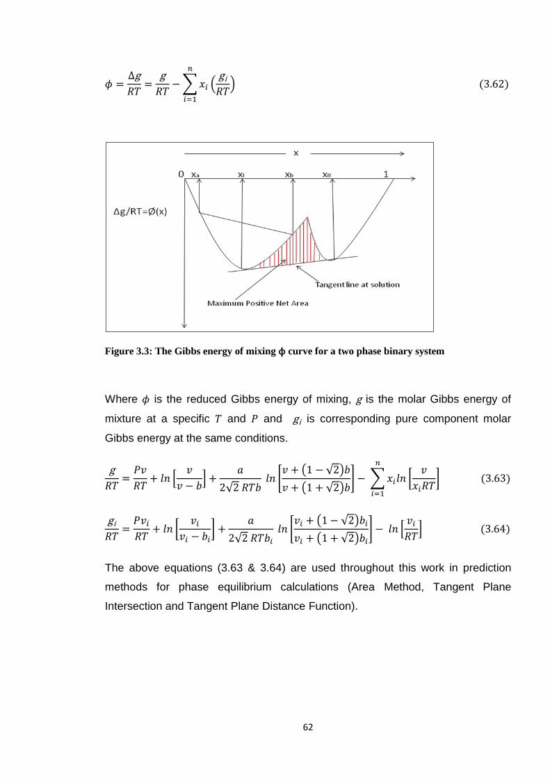
62
𝜙 =∆g
𝑅𝑇=
g
𝑅𝑇− ∑ 𝑥𝑖 (
gi
𝑅𝑇)
𝑛
𝑖=1
(3.62)
Figure 3.3: The Gibbs energy of mixing ϕ curve for a two phase binary system
Where 𝜙 is the reduced Gibbs energy of mixing, g is the molar Gibbs energy of
mixture at a specific 𝑇 and 𝑃 and gi is corresponding pure component molar
Gibbs energy at the same conditions.
g
𝑅𝑇=
𝑃𝑣
𝑅𝑇+ 𝑙𝑛 [
𝑣
𝑣 − 𝑏] +
𝑎
2√2 𝑅𝑇𝑏 𝑙𝑛 [
𝑣 + (1 − √2)𝑏
𝑣 + (1 + √2)𝑏] − ∑ 𝑥𝑖𝑙𝑛 [
𝑣
𝑥𝑖𝑅𝑇]
𝑛
𝑖=1
(3.63)
gi
𝑅𝑇=
𝑃𝑣𝑖
𝑅𝑇+ 𝑙𝑛 [
𝑣𝑖
𝑣𝑖 − 𝑏𝑖] +
𝑎
2√2 𝑅𝑇𝑏𝑖
𝑙𝑛 [𝑣𝑖 + (1 − √2)𝑏𝑖
𝑣𝑖 + (1 + √2)𝑏𝑖
] − 𝑙𝑛 [𝑣𝑖
𝑅𝑇] (3.64)
The above equations (3.63 & 3.64) are used throughout this work in prediction
methods for phase equilibrium calculations (Area Method, Tangent Plane
Intersection and Tangent Plane Distance Function).
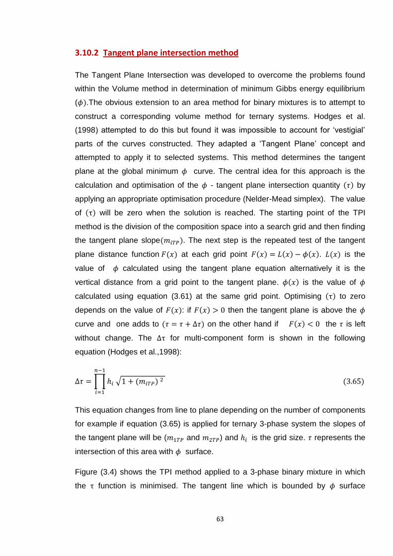
63
3.10.2 Tangent plane intersection method
The Tangent Plane Intersection was developed to overcome the problems found
within the Volume method in determination of minimum Gibbs energy equilibrium
(𝜙).The obvious extension to an area method for binary mixtures is to attempt to
construct a corresponding volume method for ternary systems. Hodges et al.
(1998) attempted to do this but found it was impossible to account for ‘vestigial’
parts of the curves constructed. They adapted a ‘Tangent Plane’ concept and
attempted to apply it to selected systems. This method determines the tangent
plane at the global minimum 𝜙 curve. The central idea for this approach is the
calculation and optimisation of the 𝜙 - tangent plane intersection quantity (𝜏) by
applying an appropriate optimisation procedure (Nelder-Mead simplex). The value
of (τ) will be zero when the solution is reached. The starting point of the TPI
method is the division of the composition space into a search grid and then finding
the tangent plane slope(𝑚𝑖𝑇𝑃). The next step is the repeated test of the tangent
plane distance function 𝐹(𝑥) at each grid point 𝐹(𝑥) = 𝐿(𝑥) − 𝜙(𝑥). 𝐿(𝑥) is the
value of 𝜙 calculated using the tangent plane equation alternatively it is the
vertical distance from a grid point to the tangent plane. 𝜙(𝑥) is the value of 𝜙
calculated using equation (3.61) at the same grid point. Optimising (τ) to zero
depends on the value of 𝐹(𝑥): if 𝐹(𝑥) > 0 then the tangent plane is above the 𝜙
curve and one adds to (𝜏 = 𝜏 + ∆𝜏) on the other hand if 𝐹(𝑥) < 0 the 𝜏 is left
without change. The ∆τ for multi-component form is shown in the following
equation (Hodges et al.,1998):
∆𝜏 = ∏ ℎ𝑖 √1 + (𝑚𝑖𝑇𝑃) 2
𝑛−1
𝑖=1
(3.65)
This equation changes from line to plane depending on the number of components
for example if equation (3.65) is applied for ternary 3-phase system the slopes of
the tangent plane will be (𝑚1𝑇𝑃 and 𝑚2𝑇𝑃) and ℎ𝑖 is the grid size. 𝜏 represents the
intersection of this area with 𝜙 surface.
Figure (3.4) shows the TPI method applied to a 3-phase binary mixture in which
the τ function is minimised. The tangent line which is bounded by 𝜙 surface
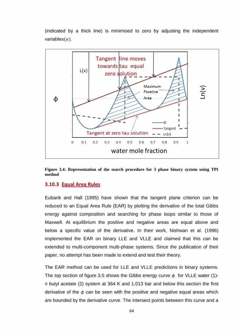
64
(indicated by a thick line) is minimised to zero by adjusting the independent
variables(𝛼).
Figure 3.4: Representation of the search procedure for 3 phase binary system using TPI
method
3.10.3 Equal Area Rules
Eubank and Hall (1995) have shown that the tangent plane criterion can be
reduced to an Equal Area Rule (EAR) by plotting the derivative of the total Gibbs
energy against composition and searching for phase loops similar to those of
Maxwell. At equilibrium the positive and negative areas are equal above and
below a specific value of the derivative. In their work, Nishwan et al. (1996)
implemented the EAR on binary LLE and VLLE and claimed that this can be
extended to multi-component multi-phase systems. Since the publication of their
paper, no attempt has been made to extend and test their theory.
The EAR method can be used for LLE and VLLE predictions in binary systems.
The top section of figure 3.5 shows the Gibbs energy curve 𝜙 for VLLE water (1)-
n butyl acetate (2) system at 364 K and 1.013 bar and below this section the first
derivative of the 𝜙 can be seen with the positive and negative equal areas which
are bounded by the derivative curve. The intersect points between this curve and a
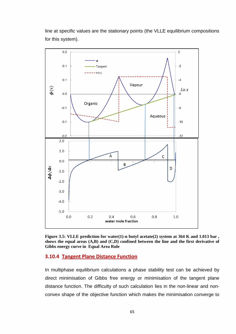
65
line at specific values are the stationary points (the VLLE equilibrium compositions
for this system).
Figure 3.5: VLLE prediction for water(1)-n butyl acetate(2) system at 364 K and 1.013 bar ,
shows the equal areas (A,B) and (C,D) confined between the line and the first derivative of
Gibbs energy curve in Equal Area Rule
3.10.4 Tangent Plane Distance Function
In multiphase equilibrium calculations a phase stability test can be achieved by
direct minimisation of Gibbs free energy or minimisation of the tangent plane
distance function. The difficulty of such calculation lies in the non-linear and non-
convex shape of the objective function which makes the minimisation converge to
66
local rather than global minima, particularly in the vicinity of phase boundaries or
near critical points. Since Michelsen's valuable achievement in finding the
stationary points of the TPDF, several attempts have been made to find these
stationary points such as: interval Newton methods (e.g., Gecegormez and
Demirel, 2005, Xu et al. ,2005), the homotopy continuation method (Kangas et
al.,2011; Sun and Seider,1995), branch and bound methods(McDonald and
Floudas,1995) and the tunnelling method (Nichita et al.,2002 ; Nichita and Gomez,
2009), in general all these global methods have shortcomings in finding all the
roots of the TPDF as the final solutions obtained rely on the initial values. The
stability test results can be used for initialising the phase split calculation or
validating the results obtained from flash calculations.
Malinen, et al. (2012) recently used the modified Newton homotopy based method
in finding the stationary points of TPDF for binary and ternary LLE systems
utilising NRTL and UNIQUAC excess Gibbs energy models in describing those
systems. They claimed that the starting value does not have any effect on finding
all the real roots of the TPDF function. However they have not indicated the
applicability of this method on the VLLE ternary and quaternary systems using
EOS.
Assuming a mixture at constant temperature and pressure with an overall
composition 𝑧 splits to a number of phases at equilibrium, thermodynamically the
Gibbs free energy will be at the minimum level. In order to perform stability test
analysis on this mixture, the Tangent Plane Distance function as defined by
equation (3.60) in the form of chemical potential (Michelsen 1982 a) must be
globally optimised with respect to composition 𝑦𝑖 subject to equality constraint in
each phase:
∑ 𝑦𝑖 = 1
𝑛𝑐
𝑖
(3.66)
0 ≤ 𝑦𝑖 ≤ 1 (𝑖 = 1,2, … 𝑛𝑐)
The mole fraction 𝑦𝑖 is the decision variable in the phase stability test, if the global
minimum of TPDF < 0 the mixture is unstable, else the system is stable. It is more
67
convenient to express the TPDF in term of fugacity coefficients, therefore equation
(3.60) can be written as:
𝐹(𝑦)
𝑅𝑇= ∑ 𝑦𝑖(𝑙𝑛𝑦𝑖 + 𝑙𝑛𝜙𝑖(𝑦) − 𝑙𝑛𝑧𝑖 − 𝑙𝑛𝜙𝑖(𝑧))
𝑖
(3.67)
The stationary criterion is:
(𝑙𝑛𝑦𝑖 + 𝑙𝑛𝜙𝑖(𝑦) − 𝑙𝑛𝑧𝑖 − 𝑙𝑛𝜙𝑖(𝑧)) = 𝑘 (3.68)
Introducing a new variable 𝑌𝑖 = exp (−𝑘)𝑦𝑖 , 𝑌𝑖 can be interpreted as mole
numbers of component 𝑖, Michelsen showed that equation (3.67) can be written
as:
𝑇𝑃𝐷𝐹(𝑌) = 1 + ∑ 𝑌𝑖[(𝑙𝑛𝑌𝑖 + 𝑙𝑛𝜙𝑖(𝑌) − 𝑙𝑛𝑧𝑖 − 𝑙𝑛𝜙𝑖(𝑧)) − 1]𝑛𝑐𝑖 (3.69)
Where 𝑦𝑖 = 𝑌𝑖/ ∑ 𝑌𝑖𝑛𝑐𝑖
The optimisation problem is minimising the TPDF function for constrained mole
fraction as independent variable 0 ≤ 𝑦𝑖 ≤ 1 , when the objective function (TPDF)
is at minimum value, 𝑦 = 𝑦∗ are the stationary points and the equation (3.67) takes
the following form:
(𝑙𝑛𝑦𝑖∗ + 𝑙𝑛𝜙𝑖(𝑦∗) − 𝑙𝑛𝑧𝑖 − 𝑙𝑛𝜙𝑖(𝑧)) = 𝑘𝑖
∗ (3.70)
Geometrically, 𝑘𝑖∗ is the distance between two hyper-planes tangent to the Gibbs
energy surface and to the tangent at feed composition. A system at a constant
temperature, pressure and feed composition is stable if 𝑘𝑖∗ ≥ 0 , if it is a negative
value, the phase is unstable and splits into two or more stable phases. As shown
by Michelsen (1982 a) the direct iteration scheme or any minimisation technique
for 𝑘∗ objective function can be used.
Initialisation is required for all the minimisation techniques for multi-phase
equilibria; some methods split the calculation into two main steps; performing two
phases stability test and using the results to initialise the three phase flash
computation.
It is acknowledged that a distinction exists between correlating the experimental
data to produce the model constants and using these values to predict data for

68
other conditions. In the field of VLE, there is sufficient published data available for
correlation of measured data to be carried out and the correlated theoretical
parameters to be used to predict and compare to other measured data. However
with reference to VLLE the basic problem in this work was that, for the relatively
complex systems measured, the amount of data available was limited to the
results of one laboratory. Thus the correlated data have been used to produce
methods for each system whereby at a given temperature and pressure the phase
equilibria can be predicted. This is demonstrated in this work using the measured
data that are available. As will be stated in the suggestions for future work, more
physical measurement is required to fully establish the predictive abilities of the
work on which this thesis is based.
3.11 Methods of initialisation
3.11.1 Initialisation techniques used in stability test
The initialisation procedure for any phase equilibrium calculations (stability test,
VLE, and VLLE flash calculation) depend on the selected minimisation method, for
instance with Nichita and Gomez (2009) their tunnelling method is based on
random multi-starting points. Michelsen and Sun and Seider (1995) suggested
the following equations:
𝑌𝑖 = 𝑧𝑖𝐾𝑖 (3.71 𝑎)
𝑌𝑖 = 𝑧𝑖/𝐾𝑖 (3.71 𝑏)
The equilibrium constants 𝐾𝑖 are obtained from the Wilson empirical relation:
𝐾𝑖 =𝑃𝑐𝑖
𝑃𝑒𝑥𝑝 [5.3727(1 + 𝜔𝑖) (1 −
𝑇𝑐𝑖
𝑇)] (3.72)
The above equations can be used for initialisation when the mutual solubility of
one component in the mixture is not very small. If the solubility value is close to the
phase boundaries surface, a different procedure is performed. Many researchers
have taken advantage from step by step phase calculations by starting from the
stability test on one phase with overall composition as a first step then using the
69
results to initialise two phase calculations and so on ( Nichita et al., 2002). In the
initialisation for three phases split calculations for a number of hydrocarbon
mixtures, Li and Firoozabadi (2012) have used direct Newton method and two
phase stability test based on the Rachford Rice equations. However many of these
methods may fail in the critical region or close to the phase boundaries, especially
when applied to complex highly non-ideal heterogeneous mixtures.
3.11.2 Direct initialisation for three phase multi component systems
This research adapted a robust and efficient initialisation method for three phase
flash calculation, based on combining the use of activity coefficient model
(UNIQUAC) and PRSV EOS with WS mixing rules. The objective function in this
work is based on relative volatilities calculations of the component 𝑖 in the mixture,
|𝑲𝒊𝒐𝒍𝒅 − 𝑲𝒊𝒏𝒆𝒘| ≥ 𝝐, 𝝐 is the tolerance to terminate the optimisation procedure
( Nelder- Mead ).
The initialisation scheme used in this work for TPI predictions for ternary and
quaternary systems can be summarised in these steps and also the diagram
shown in appendix B:
1- Set 𝑥𝑖𝑎𝑞 = 𝑧𝑖 , Calculate 𝑃𝑖
𝑠𝑎𝑡 from Antoine equation and 𝛾𝑖𝑎𝑞 from
UNIQUAC activity coefficient model
2- Estimation of organic and vapour phase compositions using equations
(3.73) and (3.74) for vapour and organic phase respectively :
𝑦𝑖 = exp[𝑙𝑛𝑥𝑖𝑎𝑞 + ln(𝛾𝑖
𝑎𝑞 + 𝑃𝑖𝑠𝑎𝑡 ) − 𝑙𝑛𝜙𝑖
𝑉(0)] (3.73)
𝑥𝑖𝑜𝑟𝑔
= exp[𝑙𝑛𝑥𝑖𝑎𝑞 + ln(𝛾𝑖
𝑎𝑞 + 𝑃𝑖𝑠𝑎𝑡 ) − ln 𝜙𝑖
𝐿(0)] (3.74)
Where 𝜙𝑖𝑉(0)
is pure vapour fugacity coefficient of component 𝑖 , equal to
1.0 for the systems with low pressure and 𝜙𝑖𝐿(0)
is pure liquid fugacity
coefficient of component 𝑖 assumed to be 𝑃𝑖𝑠𝑎𝑡/𝑃 , 𝑃 is total pressure .
3- Calculating the fugacity coefficients in all phases using the PRSV EOS with
WS mixing rules. The equilibrium ratio can be obtained from equation:

70
𝐾𝑖,𝑜𝑟𝑔 =𝜙𝑖
𝑜𝑟𝑔
𝜙𝑖𝑣 ; 𝐾𝑖,𝑎𝑞 =
𝜙𝑖𝑎𝑞
𝜙𝑖𝑣 (3.75)
4- Using the overall and component material balance equations, setting the
Rachford Rice equation (3.76) as the objective function to be minimised to
obtain 𝜃𝑜𝑟𝑔 𝑎𝑛𝑑 𝜃𝑎𝑞 fractions of molar flow rate of organic and aqueous
liquid phase with respect to the overall feed. The Nelder Mead optimisation
used with the constrained value of both flow rate 0 ≥ 𝜃𝑜𝑟𝑔 𝑎𝑛𝑑 𝜃𝑎𝑞 ≤ 1 ,
the compositions of organic, aqueous and vapour phase are calculated.
∑ 𝑥𝑖,𝑜𝑟𝑔 −
𝑛𝑐
𝑖=1
∑ 𝑦𝑖 = 0
𝑛𝑐
𝑖=1
, [∑ 𝑥𝑖,𝑎𝑞
𝑛𝑐
𝑖=1
] − 1 = 0 (3.76)
5- Calculating the organic , aqueous and vapour phase compositions using
VLLE flash equations
6- Re-estimating new values for fugacity coefficients (𝜙𝑖) and relative
volatilities (𝐾𝑖) compare these values with the old values, the criterion to
stop is 𝜀 = 0.00001 otherwise replace the (𝐾𝑖) with the new values and go
to step 3.
This initialisation method has been used throughout this work in an attempt to
overcome the sensitivity of the TPI to initial values.
3.12 The Nelder –Mead simplex
The Nelder-Mead simplex is the most widely used method for non-linear function
optimisations in the fields of chemical engineering and chemistry. This simplex
minimises function values in a direct search of 𝑛 variables without need for the
derivative of the function. The algorithm evaluates the value of a function 𝑓(𝑥) for
𝑘 number of iterations along with regeneration of the new value of variables by
using coefficient factors (reflection, expansion, contraction and shrinkage). The
standard values chosen for these coefficients are (1, 2, 0.5 and 0.5) respectively.
The largest value of 𝑓(𝑥) is rejected and the variables replaced with the new
values, this process creates a sequence of variable values for which the value of
71
𝑓(𝑥) will be at the minimum. Nelder-Mead is unconstrained minimisation which
strongly relies on the initial values.
In order to find the Best variables (B) to satisfy the 𝑓(𝑥1) ≤ 𝑓(𝑥2) ≤ ⋯ ≤ 𝑓(𝑥𝑛+1),
the procedure is to move away from the Worst values (W) to Good values (G) by
taking the steps below (appendix C shows a diagram of the Nelder-Mead simplex):
1. Compute the initial simplex from the starting values and their function
values; sort the variable and the coordinate in 𝑓(𝐵), 𝑓(𝐺), 𝑓(𝑊) in
ascending order from best to worst.
2. Compute the centroid: 𝑀 = (𝐵 + 𝐺)/2, Reflection; 𝑅 = 𝑀 + (𝑀 − 𝑊) =
2𝑀 − 𝑊 and the function value 𝑓(𝑅).
3. If 𝑓(𝑅) < 𝑓(𝐺) then preform one of these cases :
4. First case: if 𝑓(𝐵) < 𝑓(𝑅) then replace 𝑊 with 𝑅 , else compute
Expansion: 𝐸 = 𝑅 + (𝑅 − 𝑀) = 2𝑅 − 𝑀 and 𝑓(𝐸) , if 𝑓(𝐸) < 𝑓(𝐵) then
replace 𝑊 with 𝐸 , else replace 𝑊 with 𝑅.
5. Second case: if 𝑓(𝑅) < 𝑓(𝑊) then replace 𝑊 with 𝑅, compute Contraction:
𝐶 = (𝑊 + 𝑀)/2 or 𝐶 = (𝑀 + 𝑅)/2 and 𝑓(𝐶) , if 𝑓(𝐶) < 𝑓(𝑊) then replace
𝑊 with 𝐶 , else compute Shrink and 𝑓(𝑆); replace 𝑊 with 𝑆 , replace 𝐺
with 𝑀 .
6. The procedure continuously produces a sequence of 𝑓(𝑥) and the criterion
to terminate the search is when the simplex size is smaller than the
tolerance otherwise return to step 2.
Nelder and Mead published their simplex in 1965 and their method of minimisation
continues to be popular and broadly used in several practical fields. The main
advantages of this simplex are: it is easy to use and can be applied to optimise
multi-dimensional complex problems (multi-variable non-linear function).
However the disadvantage in some cases it might not converge to a global
minimum like some other methods (Newton’s method).
The Nelder-Mead optimisation simplex is widely used in the field of
thermodynamic modelling of phase equilibria particularly in the correlation of VLE,

72
LLE, and VLLE to obtain the model parameters. This simplex can also be used in
the minimization of Gibbs free energy. Throughout their work, Hodges et al.(1997
and 1998) used the Nelder-Mead method in a series of correlations and
predictions for binary and ternary VLE, LLE and VLLE calculations using Gibbs
energy minimisation as suggested by Michelson(1982) in the form of the Tangent
Plane Intersection method. In the correlation and prediction of VLE for binary
systems of alcohol-alcohol and alcohol-water at atmospheric pressure, Yan et al.
(1999) and Li et al. (2000) also used Nelder-Mead successfully. To obtain
UNIQUAC and NRTL parameters for the partially miscible ternary mixture of
ethanol-water-1-butanol at isobaric pressure, Kosuge and Iwakabe (2005) have
utilised Nelder-Mead. In modelling of three-phase vapour-liquid-liquid equilibria for
a natural gas system rich in nitrogen using the SRK and PCSAFT equations of
state, Justo-Garcia et al. (2010) have also used the minimisation simplex of
Nelder-Mead with convergence accelerated by the Wegstein algorithm. Garcia-
Flores et al. (2013) correlated liquid-liquid equilibria for ternary and quaternary
systems of representative compounds of gasoline + methanol at atmospheric
pressure using NRTL and UNIQUAC activity coefficient models; they also used
Nelder-Mead in their method. In optimisation of the biodiesel purification process
by Pinheiro et al. (2014) Nelder-Mead was used in the correlation of liquid-liquid
equilibrium for a ternary system of methanol (1)-water (2)-biodiesel (3) at
temperatures of 293.15 and 313.15 K and atmospheric pressure with UNIQUAC ,
NRTL and UNIFAC activity coefficient models .
Several studies have recently indicated that whilst the method has its drawbacks
e.g. the simplex might be trapped in local minima due to initial starting values, its
use is well established in the field and it requires no equation derivatives. Many
researchers have developed new ideas in an attempt to improve on the drawbacks
or deficiencies in NMS. Gao and Han (2010) implemented a method in which the
expansion, contraction and shrink parameters depend on the dimensions of the
optimisation problem. Pham and Wilamowski (2011) incorporated a Quasi gradient
method with the Nelder Mead simplex which approximates gradients of a function
in the vicinity of a simplex by using numerical methods. They have demonstrated
an improvement in the Nelder Mead algorithm performance for multi-variable
functions in their application. In a further study by Wanga and Shoup (2011) on
73
parameter sensitivity of the Nelder Mead for unconstrained optimisation, they
discovered that the standard values for NMS coefficients are not always the best
values. They claimed that the simplex performs more efficiently with the obtained
values.
When these modifications became available, this work had already implemented
the unmodified established Nelder-Mead simplex in optimisation methods in
correlation and predictions calculations and therefore did not investigate the
modified version. There was also significant experience available from the work of
Hodges et al., (1997, 1998) and Younis et al., (2007).

74
4. Results and discussion
4.1 Binary Systems Results
A range of binary homogeneous and heterogeneous systems were modelled
using PRSV EOS combined with WSMR using the UNIQUAC activity coefficient
equation. The VLE isobaric and isothermal data have been used to test the
suitability of the PRSV model in representing non-ideality in heterogeneous
systems.
The VLE binary homogeneous systems consist of isothermal and isobaric data for:
A- Methanol-water
1. VLE isothermal at temperatures: 25, 50, 65 and 1000C.
2. VLE isobaric at pressure: 760 mmHg.
B- Ethanol-water
1. VLE isothermal at temperatures: 20, 30, 40, 50, 60 and 700C.
2. VLE isobaric at atmospheric pressure.
C- 1-Propanol-water
1. VLE isothermal at temperature: 79.800C.
2. VLE isobaric at atmospheric pressure.
The VLE binary heterogeneous systems include isothermal and isobaric data for:
A- Water-n-butanol
1. VLE isothermal at temperature: 350C.
2. VLE isobaric at atmospheric pressure
B- Methyl ethyl ketone- water
1. VLE isothermal at temperature 73.800C.
2. VLE isobaric at atmospheric pressure
C- Water-hexanol
1. VLE isothermal at temperature 210C.
2. VLE isobaric at atmospheric pressure.

75
The Area Method and Tangent Plane Intersection predicted models were used on
binary LLE for the systems (1-butanol-water, ethyl acetate-water) and the TPI for
VLLE systems (water-n-butyl acetate, ethyl acetate-water, and n-butanol-water).
The parameters obtained from the correlation of the experimental data and these
data were acquired from DECHEMA Chemistry Data Series (1977- 1991).
The results for VLE 𝑃𝑥𝑦 isothermal in this work are compared to the results using
the WSMR package and the observation shows the model in our work is superior
on Sandler’s results.
The bubble point calculation was carried out for some binary 𝑃𝑥𝑦 and 𝑇𝑥𝑦 data
using the objective function: Absolute Average Deviations (AAD) for vapour
composition and bubble point pressure and temperature.
𝐴𝐴𝐷 =∑[|𝑒𝑥𝑝 − 𝑐𝑎𝑙𝑐|]/𝑒𝑥𝑝
𝑁𝑜. 𝑑𝑎𝑡𝑎 𝑝𝑜𝑖𝑛𝑡𝑠 (4.1)
The results are tabulated below:
4.1.1 VLE Homogeneous systems
A. methanol (1)-water (2)
1- 𝑃𝑥𝑦 methanol (1)-water (2) at temperatures: 25, 50, 65 and 1000C

76
Table 4.1: VLE bubble point calculation for methanol (1)-water (2) isothermal binary system
at 25, 50, 65 and 1000C using PRSV with WSMR through UNIQUAC
Temperature experimental calculated
x1 y1 P mmHg y1 P mmHg
25
0 C
0.1204 0.5170 43.92 0.5344 45.50 0.2039 0.6530 56.07 0.6512 56.23 0.2919 0.7295 66.04 0.7248 65.50 0.3981 0.7895 75.39 0.7862 75.20 0.4831 0.8260 82.32 0.8252 82.40 0.5349 0.8440 86.29 0.8465 86.70 0.5871 0.8645 90.54 0.8666 91.01 0.6981 0.9040 99.63 0.9063 100.26 0.8023 0.9390 108.35 0.9407 109.17 0.8522 0.9550 113.11 0.9564 113.54
50
0 C
0.0486 0.2741 119.50 0.2730 121.39 0.1218 0.4741 157.00 0.4767 157.26 0.1478 0.5220 169.10 0.5232 168.36 0.2131 0.6294 196.00 0.6106 193.50 0.2693 0.7106 217.10 0.6655 212.78 0.3252 0.7580 236.60 0.7092 230.46 0.5143 0.8203 283.00 0.8166 284.34 0.6219 0.8654 306.40 0.8640 313.41 0.7083 0.9007 324.10 0.8984 336.75 0.8037 0.9406 348.00 0.9337 362.85 0.9007 0.9627 373.50 0.9675 389.93 0.9461 0.9736 391.10 0.9826 402.82
65
0 C
0.0000 0.0000 187.54 0.0000 187.60 0.0854 0.3926 292.72 0.4057 291.54 0.0874 0.4018 294.04 0.4107 293.50 0.1328 0.4963 337.21 0.5020 333.83 0.1816 0.5718 377.29 0.5688 369.80 0.2586 0.6512 429.60 0.6412 416.20 0.4920 0.7842 544.83 0.7799 526.31 0.5815 0.8242 583.87 0.8245 567.55 0.7043 0.8747 634.71 0.8836 628.27 0.8028 0.9180 680.39 0.9275 680.54 0.9030 0.9605 727.27 0.9662 733.47 1.0000 1.0000 774.95 1.0000 776.40
10
00C
0.0022 0.0192 782.52 0.0162 770.81
0.0110 0.0860 828.40 0.0753 813.31
0.0350 0.1910 927.20 0.2002 919.76
0.0530 0.2450 1003.20 0.2700 991.41
0.0740 0.3130 1071.60 0.3343 1067.19
0.1210 0.4340 1238.80 0.4367 1211.29
0.1630 0.4960 1322.40 0.4995 1316.47
0.2810 0.6190 1535.20 0.6109 1537.34
0.3520 0.6620 1624.40 0.6579 1641.43
0.5220 0.7500 1884.80 0.7558 1870.11
0.6060 0.7920 2029.20 0.8041 1989.90
0.6670 0.8240 2112.80 0.8397 2084.23
0.8260 0.9110 2340.80 0.9286 2367.26
0.9360 0.9690 2508.00 0.9762 2572.73
0.9460 0.9760 2530.80 0.9795 2588.38
0.9580 0.9810 2530.80 0.9834 2605.51
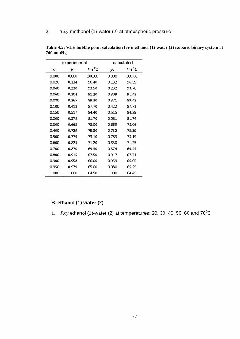
77
2- 𝑇𝑥𝑦 methanol (1)-water (2) at atmospheric pressure
Table 4.2: VLE bubble point calculation for methanol (1)-water (2) isobaric binary system at
760 mmHg
experimental calculated
x1 y1 Tin 0C y1 Tin
0C
0.000 0.000 100.00 0.000 100.00
0.020 0.134 96.40 0.132 96.59
0.040 0.230 93.50 0.232 93.78
0.060 0.304 91.20 0.309 91.43
0.080 0.365 89.30 0.371 89.43
0.100 0.418 87.70 0.422 87.71
0.150 0.517 84.40 0.515 84.29
0.200 0.579 81.70 0.581 81.74
0.300 0.665 78.00 0.669 78.06
0.400 0.729 75.30 0.732 75.39
0.500 0.779 73.10 0.783 73.19
0.600 0.825 71.20 0.830 71.25
0.700 0.870 69.30 0.874 69.44
0.800 0.915 67.50 0.917 67.71
0.900 0.958 66.00 0.959 66.05
0.950 0.979 65.00 0.980 65.25
1.000 1.000 64.50 1.000 64.45
B. ethanol (1)-water (2)
1. 𝑃𝑥𝑦 ethanol (1)-water (2) at temperatures: 20, 30, 40, 50, 60 and 700C
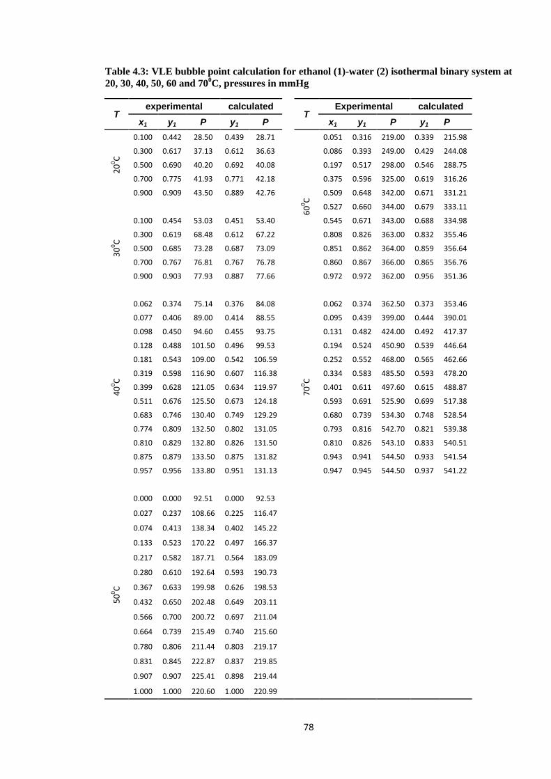
78
Table 4.3: VLE bubble point calculation for ethanol (1)-water (2) isothermal binary system at
20, 30, 40, 50, 60 and 700C, pressures in mmHg
T experimental calculated
T
Experimental calculated
x1 y1 P y1 P
x1 y1 P y1 P 2
00C
0.100 0.442 28.50 0.439 28.71
60
0C
0.051 0.316 219.00 0.339 215.98
0.300 0.617 37.13 0.612 36.63
0.086 0.393 249.00 0.429 244.08
0.500 0.690 40.20 0.692 40.08
0.197 0.517 298.00 0.546 288.75
0.700 0.775 41.93 0.771 42.18
0.375 0.596 325.00 0.619 316.26
0.900 0.909 43.50 0.889 42.76
0.509 0.648 342.00 0.671 331.21
0.527 0.660 344.00 0.679 333.11
30
0 C
0.100 0.454 53.03 0.451 53.40
0.545 0.671 343.00 0.688 334.98
0.300 0.619 68.48 0.612 67.22
0.808 0.826 363.00 0.832 355.46
0.500 0.685 73.28 0.687 73.09
0.851 0.862 364.00 0.859 356.64
0.700 0.767 76.81 0.767 76.78
0.860 0.867 366.00 0.865 356.76
0.900 0.903 77.93 0.887 77.66
0.972 0.972 362.00 0.956 351.36
40
0 C
0.062 0.374 75.14 0.376 84.08
7
00 C
0.062 0.374 362.50 0.373 353.46
0.077 0.406 89.00 0.414 88.55
0.095 0.439 399.00 0.444 390.01
0.098 0.450 94.60 0.455 93.75
0.131 0.482 424.00 0.492 417.37
0.128 0.488 101.50 0.496 99.53
0.194 0.524 450.90 0.539 446.64
0.181 0.543 109.00 0.542 106.59
0.252 0.552 468.00 0.565 462.66
0.319 0.598 116.90 0.607 116.38
0.334 0.583 485.50 0.593 478.20
0.399 0.628 121.05 0.634 119.97
0.401 0.611 497.60 0.615 488.87
0.511 0.676 125.50 0.673 124.18
0.593 0.691 525.90 0.699 517.38
0.683 0.746 130.40 0.749 129.29
0.680 0.739 534.30 0.748 528.54
0.774 0.809 132.50 0.802 131.05
0.793 0.816 542.70 0.821 539.38
0.810 0.829 132.80 0.826 131.50
0.810 0.826 543.10 0.833 540.51
0.875 0.879 133.50 0.875 131.82
0.943 0.941 544.50 0.933 541.54
0.957 0.956 133.80 0.951 131.13
0.947 0.945 544.50 0.937 541.22
50
0C
0.000 0.000 92.51 0.000 92.53
0.027 0.237 108.66 0.225 116.47
0.074 0.413 138.34 0.402 145.22
0.133 0.523 170.22 0.497 166.37
0.217 0.582 187.71 0.564 183.09
0.280 0.610 192.64 0.593 190.73
0.367 0.633 199.98 0.626 198.53
0.432 0.650 202.48 0.649 203.11
0.566 0.700 200.72 0.697 211.04
0.664 0.739 215.49 0.740 215.60
0.780 0.806 211.44 0.803 219.17
0.831 0.845 222.87 0.837 219.85
0.907 0.907 225.41 0.898 219.44
1.000 1.000 220.60 1.000 220.99

79
2. 𝑇𝑥𝑦 ethanol (1)-water (2) at atmospheric pressure
Table 4.4: VLE bubble point calculation for ethanol (1)-water (2) isobaric binary system at
760 mmHg
experimental calculated
x1 y1 Tin 0C y1 Tin
0C
0.0190 0.1700 95.50 0.1729 95.22
0.0721 0.3891 89.00 0.3862 88.32
0.0966 0.4375 86.70 0.4330 86.65
0.1238 0.4704 85.30 0.4694 85.33
0.1661 0.5089 84.10 0.5080 83.94
0.2337 0.5445 82.70 0.5482 82.56
0.2608 0.5580 82.30 0.5606 82.15
0.3273 0.5826 81.50 0.5875 81.35
0.3965 0.6122 80.70 0.6134 80.68
0.5079 0.6564 79.80 0.6567 79.80
0.5198 0.6599 79.70 0.6616 79.72
0.5732 0.6841 79.30 0.6848 79.38
0.6763 0.7385 78.74 0.7359 78.84
0.7472 0.7815 78.41 0.7775 78.58
0.8943 0.8943 78.15 0.8884 78.45
C. 1- propanol (1)-water (2)
In order to test the PRSV+WSMR model on more complex systems, with higher
polarity than systems previously tested 1-propanol (1)-water (2) was selected.
Further tests were carried out using Sandler’s programme (Orbey & Sandler,
1998) (This programme is only available for isothermal conditions). When
comparing the results obtained using their programme with those produced by this
work it shows that the model can cope with highly non-ideal polar systems and
therefore our model is appropriate in representing such complex systems.

80
1. 𝑃𝑥𝑦 1-propanol (1)-water (2) at temperature 79.800C
Table 4.5: VLE bubble point calculation for 1-propanol (1)-water (2) isothermal binary
system at 79.80 0C
T experimental
Calculated this work
calculated Sandler's
programme
x1 y1 P mmHg y1 P mmHg y1 P mmHg
79
.80
0C
0.0000 0.0000 352.60 0.0000 352.37 0.0002 350.28
0.0856 0.3542 530.00 0.3580 518.87 0.3588 525.90
0.1558 0.3765 539.60 0.3962 541.83 0.3769 536.49
0.3012 0.4060 547.00 0.4080 546.98 0.3967 543.45
0.4114 0.4201 548.10 0.4216 548.49 0.4224 546.33
0.4202 0.4234 548.50 0.4234 548.52 0.4250 546.38
0.4287 0.4287 549.70 0.4252 548.52 0.4275 546.39
0.5556 0.4376 545.70 0.4661 543.67 0.4749 541.66
0.5782 0.4642 541.70 0.4763 541.52 0.4854 539.66
0.7390 0.5649 506.60 0.5817 510.50 0.5853 511.71
0.8201 0.6428 479.20 0.6644 482.41 0.6614 485.65
1.0000 1.0000 374.60 1.0000 380.96 0.9997 378.60
2. 𝑇𝑥𝑦 1-propanol (1)-water (2) at atmospheric pressure
Table 4.6: VLE bubble point calculation for 1-propanol (1)-water (2) isobaric binary system
at 760 mmHg
experimental calculated
x1 y1 Tin 0C y1 Tin
0C
0.0000 0.0000 100.00 0.0000 100.00 0.0500 0.3481 89.30 0.3187 90.54 0.1000 0.3759 88.38 0.3846 88.38 0.1500 0.3858 88.10 0.4021 87.86 0.2000 0.3922 87.95 0.4062 87.75 0.2500 0.3999 87.81 0.4072 87.73 0.3000 0.4065 87.72 0.4089 87.71 0.3500 0.4139 87.65 0.4130 87.67 0.4000 0.4202 87.62 0.4202 87.64 0.4500 0.4397 87.62 0.4310 87.64 0.5000 0.4490 87.65 0.4455 87.70 0.5500 0.4667 87.77 0.4642 87.84 0.6000 0.4878 87.98 0.4873 88.08 0.6500 0.5239 88.31 0.5156 88.45 0.7000 0.5467 88.79 0.5498 88.97 0.7500 0.5834 89.40 0.5911 89.66 0.8000 0.6300 90.24 0.6411 90.55 0.8500 0.6917 91.40 0.7023 91.69 0.9000 0.7690 92.87 0.7783 93.13 0.9500 0.8689 94.75 0.8746 94.95 1.0000 1.0000 97.12 1.0000 97.26
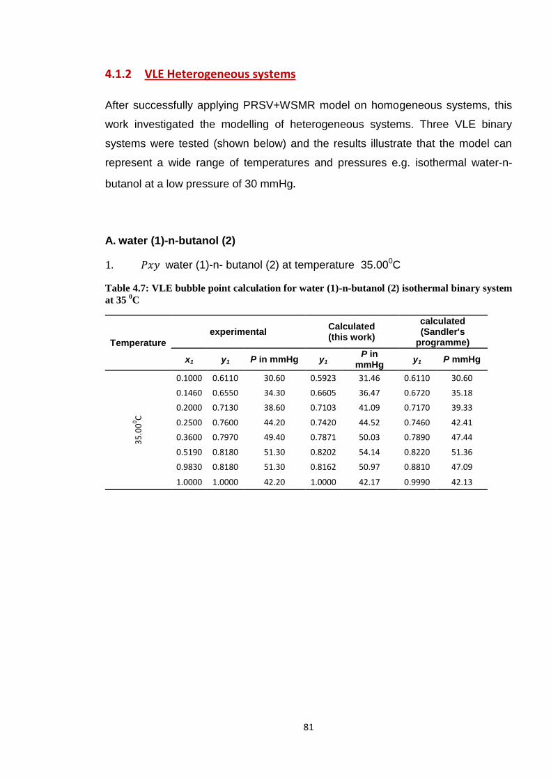
81
4.1.2 VLE Heterogeneous systems
After successfully applying PRSV+WSMR model on homogeneous systems, this
work investigated the modelling of heterogeneous systems. Three VLE binary
systems were tested (shown below) and the results illustrate that the model can
represent a wide range of temperatures and pressures e.g. isothermal water-n-
butanol at a low pressure of 30 mmHg.
A. water (1)-n-butanol (2)
1. 𝑃𝑥𝑦 water (1)-n- butanol (2) at temperature 35.000C
Table 4.7: VLE bubble point calculation for water (1)-n-butanol (2) isothermal binary system
at 35 0C
Temperature
experimental Calculated (this work)
calculated (Sandler's
programme)
x1 y1 P in mmHg y1 P in
mmHg y1 P mmHg
35
.00
0C
0.1000 0.6110 30.60 0.5923 31.46 0.6110 30.60
0.1460 0.6550 34.30 0.6605 36.47 0.6720 35.18
0.2000 0.7130 38.60 0.7103 41.09 0.7170 39.33
0.2500 0.7600 44.20 0.7420 44.52 0.7460 42.41
0.3600 0.7970 49.40 0.7871 50.03 0.7890 47.44
0.5190 0.8180 51.30 0.8202 54.14 0.8220 51.36
0.9830 0.8180 51.30 0.8162 50.97 0.8810 47.09
1.0000 1.0000 42.20 1.0000 42.17 0.9990 42.13
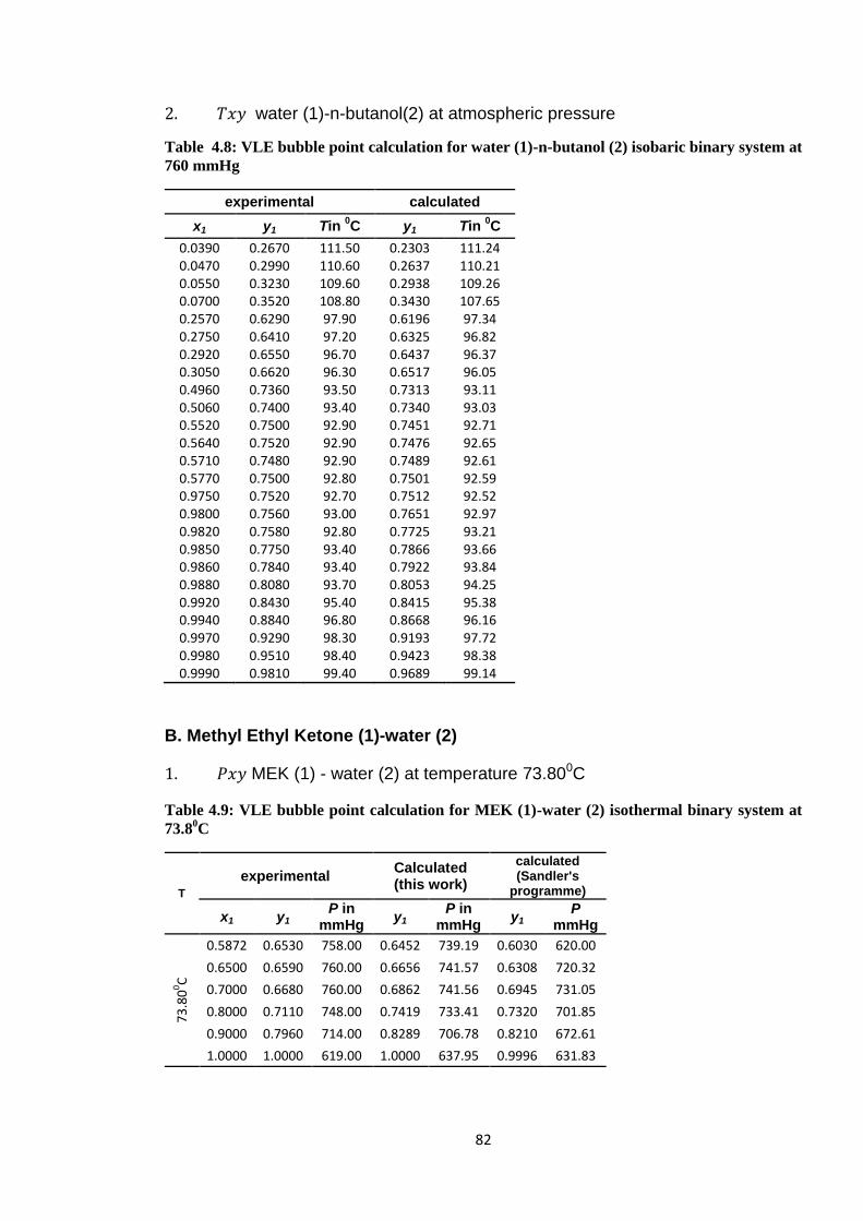
82
2. 𝑇𝑥𝑦 water (1)-n-butanol(2) at atmospheric pressure
Table 4.8: VLE bubble point calculation for water (1)-n-butanol (2) isobaric binary system at
760 mmHg
experimental calculated
x1 y1 Tin 0C y1 Tin
0C
0.0390 0.2670 111.50 0.2303 111.24 0.0470 0.2990 110.60 0.2637 110.21 0.0550 0.3230 109.60 0.2938 109.26 0.0700 0.3520 108.80 0.3430 107.65 0.2570 0.6290 97.90 0.6196 97.34 0.2750 0.6410 97.20 0.6325 96.82 0.2920 0.6550 96.70 0.6437 96.37 0.3050 0.6620 96.30 0.6517 96.05 0.4960 0.7360 93.50 0.7313 93.11 0.5060 0.7400 93.40 0.7340 93.03 0.5520 0.7500 92.90 0.7451 92.71 0.5640 0.7520 92.90 0.7476 92.65 0.5710 0.7480 92.90 0.7489 92.61 0.5770 0.7500 92.80 0.7501 92.59 0.9750 0.7520 92.70 0.7512 92.52 0.9800 0.7560 93.00 0.7651 92.97 0.9820 0.7580 92.80 0.7725 93.21 0.9850 0.7750 93.40 0.7866 93.66 0.9860 0.7840 93.40 0.7922 93.84 0.9880 0.8080 93.70 0.8053 94.25 0.9920 0.8430 95.40 0.8415 95.38 0.9940 0.8840 96.80 0.8668 96.16 0.9970 0.9290 98.30 0.9193 97.72 0.9980 0.9510 98.40 0.9423 98.38 0.9990 0.9810 99.40 0.9689 99.14
B. Methyl Ethyl Ketone (1)-water (2)
1. 𝑃𝑥𝑦 MEK (1) - water (2) at temperature 73.800C
Table 4.9: VLE bubble point calculation for MEK (1)-water (2) isothermal binary system at
73.80C
T
experimental Calculated (this work)
calculated (Sandler's
programme)
x1 y1 P in
mmHg y1
P in mmHg
y1 P
mmHg
73
.80
0C
0.5872 0.6530 758.00 0.6452 739.19 0.6030 620.00
0.6500 0.6590 760.00 0.6656 741.57 0.6308 720.32
0.7000 0.6680 760.00 0.6862 741.56 0.6945 731.05
0.8000 0.7110 748.00 0.7419 733.41 0.7320 701.85
0.9000 0.7960 714.00 0.8289 706.78 0.8210 672.61
1.0000 1.0000 619.00 1.0000 637.95 0.9996 631.83
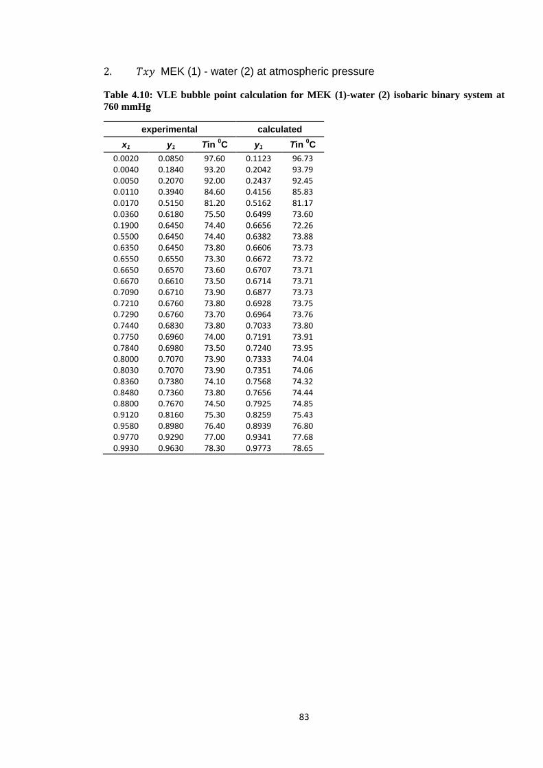
83
2. 𝑇𝑥𝑦 MEK (1) - water (2) at atmospheric pressure
Table 4.10: VLE bubble point calculation for MEK (1)-water (2) isobaric binary system at
760 mmHg
experimental calculated
x1 y1 Tin 0C y1 Tin
0C
0.0020 0.0850 97.60 0.1123 96.73 0.0040 0.1840 93.20 0.2042 93.79 0.0050 0.2070 92.00 0.2437 92.45 0.0110 0.3940 84.60 0.4156 85.83 0.0170 0.5150 81.20 0.5162 81.17 0.0360 0.6180 75.50 0.6499 73.60 0.1900 0.6450 74.40 0.6656 72.26 0.5500 0.6450 74.40 0.6382 73.88 0.6350 0.6450 73.80 0.6606 73.73 0.6550 0.6550 73.30 0.6672 73.72 0.6650 0.6570 73.60 0.6707 73.71 0.6670 0.6610 73.50 0.6714 73.71 0.7090 0.6710 73.90 0.6877 73.73 0.7210 0.6760 73.80 0.6928 73.75 0.7290 0.6760 73.70 0.6964 73.76 0.7440 0.6830 73.80 0.7033 73.80 0.7750 0.6960 74.00 0.7191 73.91 0.7840 0.6980 73.50 0.7240 73.95 0.8000 0.7070 73.90 0.7333 74.04 0.8030 0.7070 73.90 0.7351 74.06 0.8360 0.7380 74.10 0.7568 74.32 0.8480 0.7360 73.80 0.7656 74.44 0.8800 0.7670 74.50 0.7925 74.85 0.9120 0.8160 75.30 0.8259 75.43 0.9580 0.8980 76.40 0.8939 76.80 0.9770 0.9290 77.00 0.9341 77.68 0.9930 0.9630 78.30 0.9773 78.65
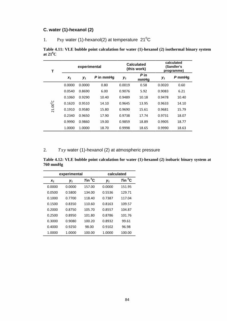
84
C. water (1)-hexanol (2)
1. Pxy water (1)-hexanol(2) at temperature 210C
Table 4.11: VLE bubble point calculation for water (1)-hexanol (2) isothermal binary system
at 210C
T
experimental Calculated (this work)
calculated (Sandler's
programme)
x1 y1 P in mmHg y1 P in
mmHg y1 P mmHg
21
.00
0C
0.0000 0.0000 0.80 0.0019 0.58 0.0020 0.60
0.0540 0.8690 6.00 0.9076 5.92 0.9083 6.21
0.1060 0.9290 10.40 0.9489 10.18 0.9478 10.40
0.1620 0.9510 14.10 0.9645 13.95 0.9633 14.10
0.1910 0.9580 15.80 0.9690 15.61 0.9681 15.79
0.2340 0.9650 17.90 0.9738 17.74 0.9731 18.07
0.9990 0.9860 19.00 0.9859 18.89 0.9905 18.77
1.0000 1.0000 18.70 0.9998 18.65 0.9990 18.63
2. 𝑇𝑥𝑦 water (1)-hexanol (2) at atmospheric pressure
Table 4.12: VLE bubble point calculation for water (1)-hexanol (2) isobaric binary system at
760 mmHg
experimental calculated
x1 y1 Tin 0C y1 Tin
0C
0.0000 0.0000 157.00 0.0000 151.95
0.0500 0.5800 134.00 0.5536 129.71
0.1000 0.7700 118.40 0.7387 117.04
0.1500 0.8350 110.60 0.8163 109.57
0.2000 0.8750 105.70 0.8557 104.87
0.2500 0.8950 101.80 0.8786 101.76
0.3000 0.9080 100.20 0.8932 99.61
0.4000 0.9250 98.00 0.9102 96.98
1.0000 1.0000 100.00 1.0000 100.00

85
Table 4.13: UNIQUAC parameters and PRSV interaction parameters and AAD for vapour
phase, temperature and pressure for VLE binary homogeneous and heterogeneous systems
(isothermal and isobaric)
System Status T in 0 C
UNIQUAC PRSV EOS
AAD
A12 A21 K12 AAD y P & T
Homogeneous systems
methanol-water
Isothermal
25 66.60 -101.97 0.1447 0.0059 0.0078
50 59.69 -94.12 0.0952 0.0167 0.0220
65 947.49 -453.31 0.2536 0.0100 0.0125
100 1805.8 -573.77 0.2989 0.0379 0.0141
Isobaric
134.93 -152.59 0.1823 0.0059 0.0015
ethanol-water
Isothermal
20 279.4 54.52 0.1713 0.0076 0.0094
30 336.47 -11.67 0.2381 0.0068 0.0064
40 152.69 69.04 0.2690 0.0079 0.0200
50 169.75 150.42 0.1988 0.0161 0.0243
60 799.04 -263.11 0.3852 0.0343 0.0249
70 760.19 -303.15 0.4177 0.0128 0.0128
Isobaric
110.37 509.03 0.0581 0.0044 0.0018
propanol-water
Isothermal 79.8 149.57 296.39 0.4148 0.0192 0.0053
Isobaric
139.60 539.83 0.3498 0.0158 0.002
Heterogeneous systems
water-n-butanol
Isothermal 35 752.91 352.05 0.4874 0.0105 0.0298
Isobaric
1497.44 184.77 0.3639 0.0190 0.0036
water-hexanol
Isothermal 21 306.64 364.73 0.2900 0.0126 0.0442
Isobaric
503.84 622.33 0.031 0.0202 0.0122
MEK-water
Isothermal 73.8 427.64 559.19 0.4129 0.0223 0.0223
Isobaric
543.70 811.01 0.3665 0.0347 0.0059
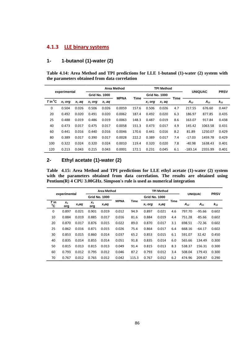
86
4.1.3 LLE binary systems
1- 1-butanol (1)-water (2)
Table 4.14: Area Method and TPI predictions for LLE 1-butanol (1)-water (2) system with
the parameters obtained from data correlation
experimental Area Method TPI Method
UNIQUAC PRSV Grid No. 1000
MPNA Time Grid No. 1000
Time T in
0C x1 org x1 aq x1 org x1 aq x1 org x1 aq A12 A21 k12
0 0.504 0.026 0.506 0.026 0.0059 157.6 0.506 0.026 4.7 217.55 676.60 0.447
20 0.492 0.020 0.491 0.020 0.0062 187.4 0.492 0.020 6.3 186.97 877.85 0.435
25 0.488 0.019 0.486 0.019 0.0063 148.3 0.487 0.019 8.6 163.07 917.84 0.438
40 0.473 0.017 0.475 0.017 0.0058 151.3 0.473 0.017 4.9 145.42 1063.58 0.431
60 0.441 0.016 0.440 0.016 0.0046 170.6 0.441 0.016 8.2 81.89 1250.07 0.429
80 0.389 0.017 0.390 0.017 0.0028 222.2 0.389 0.017 7.4 -17.03 1459.78 0.429
100 0.322 0.024 0.320 0.024 0.0010 119.4 0.320 0.020 7.8 -40.98 1638.43 0.401
120 0.213 0.043 0.215 0.043 0.0001 172.1 0.231 0.045 6.1 -183.14 2355.99 0.401
2- Ethyl acetate (1)-water (2)
Table 4.15: Area Method and TPI predictions for LLE ethyl acetate (1)-water (2) system
with the parameters obtained from data correlation. The results are obtained using
Pentium(R) 4 CPU 3.00GHz. Simpson's rule is used as numerical integration
experimental Area Method TPI Method
UNIQUAC PRSV Grid No. 1000
MPNA Time Grid No. 1000
Time T in
0C
x1 org
x1aq x1
org x1aq x1 org x1aq A12 A21 k12
0 0.897 0.021 0.901 0.019 0.012 94.9 0.897 0.021 4.6 797.70 -95.66 0.602
10 0.884 0.019 0.885 0.017 0.016 81.6 0.884 0.019 4.4 751.28 -85.66 0.602
20 0.870 0.017 0.876 0.015 0.022 89.0 0.870 0.017 3.1 698.51 -72.36 0.602
25 0.862 0.016 0.871 0.015 0.026 75.4 0.864 0.017 6.4 668.16 -64.17 0.602
30 0.853 0.015 0.860 0.014 0.037 65.2 0.853 0.015 6.1 591.07 32.42 0.450
40 0.835 0.014 0.855 0.014 0.051 91.8 0.835 0.014 6.0 565.66 134.49 0.300
50 0.815 0.013 0.815 0.013 0.049 91.4 0.815 0.013 8.3 538.37 156.31 0.300
60 0.793 0.012 0.795 0.012 0.046 87.2 0.793 0.012 3.4 508.04 179.43 0.300
70 0.767 0.012 0.765 0.012 0.042 115.3 0.767 0.012 6.2 474.96 209.87 0.290
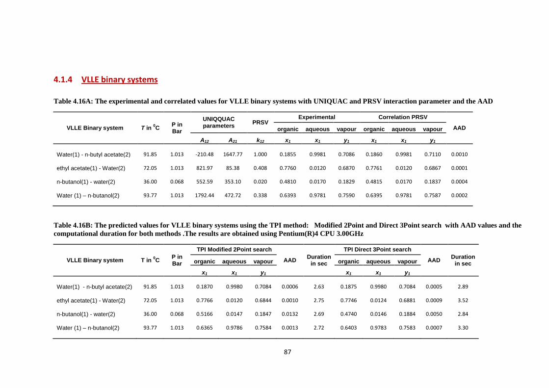
87
4.1.4 VLLE binary systems
Table 4.16A: The experimental and correlated values for VLLE binary systems with UNIQUAC and PRSV interaction parameter and the AAD
VLLE Binary system T in 0C
P in Bar
UNIQQUAC parameters
PRSV Experimental Correlation PRSV
AAD organic aqueous vapour organic aqueous vapour
A12 A21 k12 x1 x1 y1 x1 x1 y1
Water(1) - n-butyl acetate(2) 91.85 1.013 -210.48 1647.77 1.000 0.1855 0.9981 0.7086 0.1860 0.9981 0.7110 0.0010
ethyl acetate(1) - Water(2) 72.05 1.013 821.97 85.38 0.408 0.7760 0.0120 0.6870 0.7761 0.0120 0.6867 0.0001
n-butanol(1) - water(2) 36.00 0.068 552.59 353.10 0.020 0.4810 0.0170 0.1829 0.4815 0.0170 0.1837 0.0004
Water (1) – n-butanol(2) 93.77 1.013 1792.44 472.72 0.338 0.6393 0.9781 0.7590 0.6395 0.9781 0.7587 0.0002
Table 4.16B: The predicted values for VLLE binary systems using the TPI method: Modified 2Point and Direct 3Point search with AAD values and the
computational duration for both methods .The results are obtained using Pentium(R)4 CPU 3.00GHz
VLLE Binary system T in 0C
P in Bar
TPI Modified 2Point search
AAD Duration
in sec
TPI Direct 3Point search
AAD Duration
in sec organic aqueous vapour organic aqueous vapour
x1 x1 y1 x1 x1 y1
Water(1) - n-butyl acetate(2) 91.85 1.013 0.1870 0.9980 0.7084 0.0006 2.63 0.1875 0.9980 0.7084 0.0005 2.89
ethyl acetate(1) - Water(2) 72.05 1.013 0.7766 0.0120 0.6844 0.0010 2.75 0.7746 0.0124 0.6881 0.0009 3.52
n-butanol(1) - water(2) 36.00 0.068 0.5166 0.0147 0.1847 0.0132 2.69 0.4740 0.0146 0.1884 0.0050 2.84
Water (1) – n-butanol(2) 93.77 1.013 0.6365 0.9786 0.7584 0.0013 2.72 0.6403 0.9783 0.7583 0.0007 3.30
88
4.2 Discussion
This work attempts to model Phase Equilibria for highly non-ideal vapour-liquid-
liquid systems. The number of components in each phase determines the
complexity of the problem. The modelling includes VLE, LLE & VLLE binaries and
VLLE ternary and quaternary systems.
The key to the modelling lies in an ability to represent the basic thermodynamics of
the systems considered. Over the last 20 years more emphasis has been placed
on representing the thermodynamic property of fugacity through universally
applicable Equations of State (EOS). This has the advantage that all the phases
present are modelled using the same form of equation (as reviewed in chapter
2.3).
The literature survey demonstrates that systems can show deviations from ideality
and this non-ideality often arises from strong polar interactions between
molecules. The challenge is to be able to satisfactorily model this non-ideal
behaviour using an appropriate thermodynamic model. The literature survey (2.2)
shows that a range of thermodynamic models are available and these are usually
classified through representing the liquid phase fugacity in terms of an activity
coefficient model or an appropriate EOS.
As previously stated, this work investigates the applicability and effectiveness of a
particular EOS namely the PRSV + Wong Sandler Mixing Rules. Initially to
demonstrate the suitability of the proposed model (PRSV+ Wong-Sandler Mixing
Rules) and to confirm the work in this field (Ghosh and Taraphar, 1998;
Khodakarami et al., 2005; Mario and Mauricio, 2011) it is sensible to check that
the model is applicable to the VLE of binary systems showing a range of non-ideal
behaviour.
It is known that organic molecules usually show a range of positive deviations from
Raoult’s law in the presence of water. Allied to these deviations, if the organic
component and water are relatively close when boiling at a fixed pressure, there is
the possibility of the formation of minimum boiling azeotrope.

89
4.2.1 VLE binary homogeneous mixtures
Three systems have been chosen where measured VLE data are available under
isothermal and isobaric conditions. These are:
1. Methanol-Water
2. Ethanol-Water
3. 1-propanol-Water
The VLE data have been taken from DECHEMA data collection (1977). At normal
pressure the following boiling points are known:
Component B.Pt0C
methanol 65.00
ethanol 78.37
1-propanol 97.00
water 100.00
The methanol-water system does show positive deviations. When figure 4.1
( A & B) is examined the 𝑥𝑦 versus temperature & pressure plot shows “ Pinch” at
high values of 𝑥 with the fairly high difference in normal boiling points, an
azeotrope has not been formed but the behaviour of the system at high values of 𝑥
indicates deviations from ideality.
The ethanol-water system also shows positive deviation from ideality, with the
component boiling points being closer. The system shows evidence of the
formation of a minimum boiling azeotrope at values of > 0.95. This is noticeable
when observing the figure 4.2(A&B) where the 𝑥𝑦 versus 𝑇 & 𝑃 plot shows obvious
deviations from ideality.
The positive deviation from ideality for 1-propanol–water system is greater than
the methanol-water & ethanol-water systems. When the components have close
boiling points and the system clearly forms minimum boiling azeotrope behaviour
(at value of 0.41), the increase in deviation is apparently linked to an increased
carbon number in the alcohol. This highly non-ideality is visible when the 𝑥𝑦 is
plotted against 𝑇&𝑃 as shown in figure 4.3 (A&B).
90
The comparisons of experimental and correlated data obtained by using PRSV
EOS with WSMR for bubble point temperature, pressure and vapour composition
for all three systems are shown in figure 4.1, 4.2 & 4.3(C, D, E & F).
The VLE of the methanol-water system have been modelled for isothermal and
isobaric conditions using PRSV+WSMR. The results obtained show that the
Absolute Average Deviation (AAD) for the vapour phase is 0.0059 and for
pressure 0.0015 in mmHg. The VLE for the above system has been correlated at
isothermal conditions at the following temperatures: 25, 50,1000C.The results
indicate the AAD values for vapour phase and temperature are 0.0176 and 0.0141
in degree Celsius respectively. The values for each point calculations are shown in
tables: (4.1 & 4.2). Table (4.13) also displays the UNIQUAC and PRSV
parameters.
The results for the VLE of the ethanol-water system using the PRSV+WSMR
model show that the AAD in isothermal conditions for the vapour phase is 0.0044
and for pressure is 0.0018 in mmHg. Meanwhile the bubble point calculation at
isobaric conditions for the following temperatures: 20, 30, 40, 50, 60 & 700C were
carried out and the AAD for the vapour phase composition for all the data points is:
0.0143 and the AAD in temperature is 0.0163 in degree centigrade. The details for
each of the calculation results with the energy parameters for UNIQUAC activity
model and PRSV binary interaction parameters for each defined system are
presented in tables: (4.3, 4.4 & 4.13).
The performance of PRSV+WSMR remains reliable in spite of the increased
polarity, for instance the results for 1-propanol-water prove this consistency with
the previous homogenous systems. The AAD in vapour phase and pressure at
isothermal condition are 0.0195 and 0.0053 respectively. These results compare
well with those using VLE Orbey & Sandler’s (1998) programme which are 0.0205
and 0.0071 respectively. In isobaric condition the AAD in vapour phase and
temperature are 0.0158 and 0.002. The results for this system with the binary
interaction parameters are shown in table (4.5, 4.6 & 4.13).
Pervious researchers recommended the WSMR for non-ideal polar organic
systems. Orbey and Sandler (1998) and Lee et al. (2007) have examined WSMR
on a wide range of VLE binary systems e.g. 2-propanol-water & acetone-water
91
and they concluded the WSMR performance to be the best when compared to
other mixing rules e. g. Huron-Vidal & van der Waals. Other researchers have
come to the same conclusion and in a study by Ghosh et al. (1998) on VLE for
forty-three binary systems including various mixtures (organic alcohols , esters ,
ketones ,amines etc.) using WSMR , the results obtained were comparable with
DECHEMA data series. When modelling VLE for ethanol mixtures found in
alcoholic beverage production, Claudio et al. (2009) recommended the use of
WSMR to model low pressure complex mixtures.
It was noticed when fitting the model (PRSV+WSMR) incorporated with UNIQUAC
activity coefficient as excess Gibbs energy to the VLE binary data for three
homogenous systems, the results prove that the model accurately represents such
systems, therefore the WSMR were found to be satisfactory in description of
phase behaviour of non-ideal systems.
4.2.2 VLE binary heterogeneous mixtures
The 1-propanol-water is a highly non-ideal polar system when compared to other
homogenous systems. In order to be assured that PRSV EOS combined with
UNIQUAC activity coefficient through WS mixing rule can model heterogeneous
mixtures successfully; three binary systems were selected and tested for this
purpose:
1- Water-n-butanol
2- Methyl Ethyl Ketone (MEK)-water
3- Water-1-hexanol
As the interaction between unlike molecules decreases and increases for like
molecules the mixture shows a tendency to split into two liquid phases. This
behaviour occurs when the number of CH2 group increases in the alcohol
molecule and as a consequence leads to a reduction in the mutual solubility of the
alcohol in water. Heterogeneous systems form a minimum azeotrope. The
composition value for this azeotrope in water- n-butanol system is 0.74 at
temperature of 92.700C, in MEK-water system is 0.65 at temperature 73.600C and
for water-hexanol system is 0.91 at temperature 960C.
92
Observations of the correlation of VLE for highly non ideal polar systems using
PRSV EOS show the capability of this model to adequately represent the vapour
pressure for these systems. The AAD for isobaric water-n butanol is 0.0107 in
vapour mole fraction and 0.35 for the temperature. The estimated values versus
the experimental are shown in figure 4.4(C&E) and table (4.8). The AAD results for
isothermal data at 350C are 0.0075 for vapour fraction and 0.0016 for pressure (in
mmHg), the comparisons between the experimental versus calculated values are
plotted and shown in figure 4.4(D&F) and in table 4.7.
Figure 4.4(A & B) show the excellent agreement between the experimental and
correlated values for the mixture water-n-butanol VLE system and similar results
were found by Sandler et al. (1998). In a comparison study of liquid –liquid
equilibrium at low pressure using the optimised parameters for predicting a high
pressure system using WSMR and (MHV1, MHV2), the authors indicated the
WSMR results were more accurate than MHV mixing rules.
Figure 4.5(A&B) represent isobaric and isothermal binary VLE MEK-water system.
The AAD for the isobaric condition are 0.0347 and 0.0059 for vapour mole fraction
and temperature in centigrade respectively. In isothermal conditions the AAD are
0.0223 for both vapour and pressure in mmHg. The details and the values for each
calculation are tabulated in table (4.9 & 4.10). The VLE results for isobaric MEK-
water prove that the PRSV+WSMR can represent the polar and asymmetric
systems. In spite of the fact that the water –hexanol system is highly asymmetric
the results for VLE correlation using PRSV+WSMR model were in agreement with
other researchers findings (Coutsikos et al., 1995). Table 4.11 and 4.12 show the
values for the calculations with experimental data. The AAD for isobaric data are:
0.0202 and 0.0122 for vapour mole fraction and temperature in centigrade and for
isothermal data are 0.0126 and 0.442 for vapour and pressure in mmHg
respectively. Figures 4.6(A&B) show the temperature and pressure versus water
mole fraction for water-1-hexanol system, the calculated values are comparable
with experimental values. Figure 4.6(C, D, E &F) illustrate the visual comparison
between the estimated and experimental values. The graphical observation of
calculated values of vapour compositions & pressure versus experimental values
demonstrates that our model (PRSV+WSMR) produced better results than those
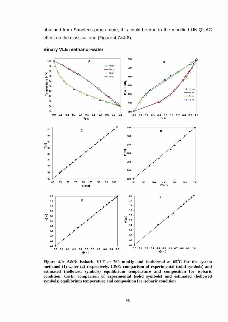
93
obtained from Sandler's programme; this could be due to the modified UNIQUAC
effect on the classical one (Figure 4.7&4.8).
Binary VLE methanol-water
Figure 4.1: A&B: isobaric VLE at 760 mmHg and isothermal at 650C for the system
methanol (1)-water (2) respectively. C&E: comparison of experimental (solid symbols) and
estimated (hollowed symbols) equilibrium temperature and composition for isobaric
condition. C&E: comparison of experimental (solid symbols) and estimated (hollowed
symbols) equilibrium temperature and composition for isobaric condition
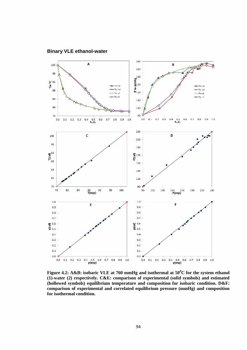
94
Binary VLE ethanol-water
Figure 4.2: A&B: isobaric VLE at 760 mmHg and isothermal at 500C for the system ethanol
(1)-water (2) respectively. C&E: comparison of experimental (solid symbols) and estimated
(hollowed symbols) equilibrium temperature and composition for isobaric condition. D&F:
comparison of experimental and correlated equilibrium pressure (mmHg) and composition
for isothermal condition.
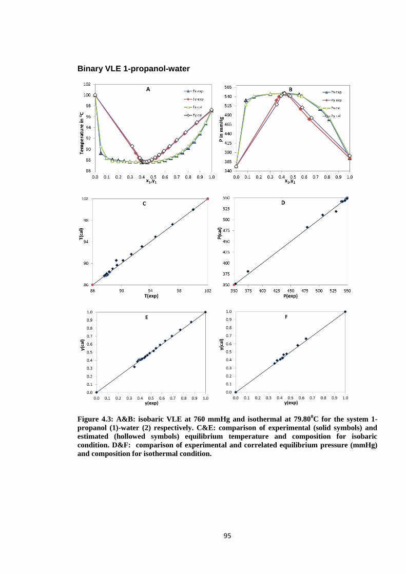
95
Binary VLE 1-propanol-water
Figure 4.3: A&B: isobaric VLE at 760 mmHg and isothermal at 79.800C for the system 1-
propanol (1)-water (2) respectively. C&E: comparison of experimental (solid symbols) and
estimated (hollowed symbols) equilibrium temperature and composition for isobaric
condition. D&F: comparison of experimental and correlated equilibrium pressure (mmHg)
and composition for isothermal condition.

96
Binary VLE water-n-butanol
Figure 4.4: A&B: isobaric VLE at 760 mmHg and isothermal at 35.00C for the system water
(1)-n-butanol (2) respectively. C&E: comparison of experimental (solid symbols) and
estimated (hollowed symbols) equilibrium temperature and composition for isobaric
condition. D&F: comparison of experimental and correlated equilibrium pressure (mmHg)
and composition for isothermal condition.

97
Binary VLE MEK-water
Figure 4.5: A&B: isobaric VLE at 760 mmHg and isothermal at 73.800C for the system MEK
(1)-water (2) respectively. C&E: comparison of experimental (solid symbols) and estimated
(hollowed symbols) equilibrium temperature and composition for isobaric condition. D&F:
comparison of experimental and correlated equilibrium pressure (mmHg) and composition
for isothermal condition.

98
Binary VLE water-hexanol
Figure 4.6: A&B: isobaric VLE at 760 mmHg and isothermal at 21.00C for the system water
(1)-1-hexanol (2) respectively. C&E: comparison of experimental (solid symbols) and
estimated (hollowed symbols) equilibrium temperature and composition for isobaric
condition. D&F: comparison of experimental and correlated equilibrium pressure (mmHg)
and composition for isothermal condition.
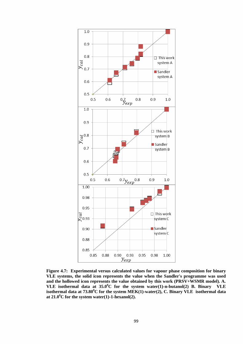
99
Figure 4.7: Experimental versus calculated values for vapour phase composition for binary
VLE systems, the solid icon represents the value when the Sandler's programme was used
and the hollowed icon represents the value obtained by this work (PRSV+WSMR model). A.
VLE isothermal data at 35.00C for the system water(1)-n-butanol(2) B. Binary VLE
isothermal data at 73.800C for the system MEK(1)-water(2), C. Binary VLE isothermal data
at 21.00C for the system water(1)-1-hexanol(2).

100
Figure 4.8: Experimental versus calculated values for pressure (mmHg) for binary VLE
systems, the solid icon represents the AD value when the Sandler's programme was used and
the hollowed icon represents the AD value obtained by this work (PRSV+WSMR model). A.
VLE isothermal data at 35.00C for the system water(1)-n-butanol(2) B. Binary VLE
isothermal data at 73.800C for the system MEK(1)-water(2), C. Binary VLE isothermal data
at 21.00C for the system water(1)-1-hexanol(2).

101
4.2.3 Conclusions on PRSV+WSMR
Generally ranges of binary VLE systems have been modelled using the PRSV +
WSMR through UNIQUAC activity coefficient as excess Gibbs energy function.
This covers the range from homogenous slightly non-ideal to strongly non-ideal
heterogeneous mixtures at low and moderate pressures and this model shows the
capability to represent these complex systems. Despite some limitations for highly
asymmetric systems, this conclusion is in line with other researchers findings. As
the size of the hydrocarbon molecule increases the system becomes more
asymmetric and one of the limitations for the WSMR is poor correlation for highly
asymmetric systems at high pressure.
One of the main considerations in discussing non-ideality in binary system is the
relative strength of the mixture bond. Thus as we consider homologous series for
ethanol, propanol, butanol in the presence of water, experimental data indicate
that the positive deviations increase as the hydrocarbon chain length increases.
The increase in the positive deviations is obviously linked to the availability of the
polar –OH group in the alcohol to the –OH group in the water molecule. The length
of the hydrocarbon chain makes the availability of the –OH group in the alcohol
much less and the mixture bond much weaker to the point where two liquid phases
can form rich in each of the separate components. The next section comprises of
the results & discussion on further tests which were carried out on PRSV+WSMR
for correlation of liquid-liquid and vapour-liquid-liquid equilibrium, for a range of
binary systems. The parameters obtained from correlation of data were used in
prediction of mutual solubility of these mixtures, applying Gibbs minimisation
techniques.

102
4.3 Prediction models for modelling binary LLE & VLLE systems
The Area Method (AM) developed by Eubank et al. (1992) and the Tangent Plane
Intersection (TPI) method developed by Hodges et al. (1998) have been applied to
two binary systems:1
1- LLE butanol-water system in the 0-1200C temperature range.
2- LLE ethyl acetate –water system in the 0-700C temperature range.
The experimental data were acquired from DECHEMA chemistry series (1977-
1991).
The prediction results for both systems are shown in table 4.14 and 4.15
respectively; the parameters used were obtained from LLE correlations using
PRSV EOS combined with the Wong Sandler mixing rules. The results obtained in
this work indicated that, for these data, both Gibbs free minimisation methods (AM
& TPI) are reliable and robust for such non-ideal binary systems.
It was observed that the AM was computationally slow compared to the TPI
method; this is due to the integration part of the calculation in a search for the
maximum positive net area (MPNA) under the Gibbs energy curve and bounded
by the tangent plane. Consequently AM was only used for LLE binary systems. It
was observed that for the butanol-water system the Gibbs energy curve flattens in
the 2 phase region as the temperature increases up to a point where the 2-phase
behaviour is almost eliminated (as shown in the figure 4.9). This change was not
so pronounced in the Gibbs energy curve for the ethyl acetate- water system.
Figure 4.10 shows the ethyl acetate mole fraction verses the Gibbs energy curve
for various temperatures. The Absolute Average Deviation (AAD) for the AM and
TPI predictions for the butanol-water system are 0.0008 and 0.0019 respectively.
The AAD for the AM and the TPI predictions in the ethyl acetate-water system are
0.0033 and 0.0004 respectively.

103
Figure 4.9: Gibbs energy curve of liquid-liquid equilibrium for 1-butanol (1)-water (2) system
at temperature range (0-120)0C
Figure 4.10: Gibbs free energy curve of liquid-liquid equilibrium for ethyl acetate (1)-water
(2) system at temperature range (0-70)0C
104
Part of this work is to test the applicability of the TPI method to VLLE binary
systems. Four binary systems were selected and correlated using PRSV EOS
combined with UNIQUAC through WSMR. The VLLE binary systems investigated
were:
1. Water- n-butyl acetate at 91.850C and 1.013 bar.
2. Ethyl acetate – water at 72.050C and 1.013 bar.
3. n-butanol - water at 36.000C and 0.068 bar.
4. Water-n-butanol at 93.770C and 1.013 bar.
Tables 4.16 (A&B) show the parameters obtained by correlating the experimental
data and the predictive values using the TPI method. The TPI search procedure is
explained in detail in the theory section (3.10.2). The search is started by defining
the grid size (1000), the process then calculates and stores the reduced Gibbs
energy of mixing (∅) at a fixed pressure and temperature. The cubic root solver
function is used to find the compressibility factor (𝑍) for PRSV EOS, to identify the
phase region (liquid or vapour). The initial starting points are selected (2, grid-1)
and the following step is the calculation of the tangent slope and ∆𝜏 at the
corresponding compositions, then (τ) is calculated and stored. The sequential
search is conducted for 𝐹(𝑥) = 𝐿(𝑥) − ∅(𝑥) , where 𝐿(𝑥) is the value of ∅ on the
tangent line at a trial composition 𝑥 , if 𝐹(𝑥) > 0 the tangent is above the ∅ curve
and τ is updated (τ = τ + ∆ τ ). The Nelder Mead simplex is used to minimise the
τ function by changing ∝ values (∝ is the length variable which starts from feed
composition(𝑧)). The solution for the minimisation procedure is the stationary
points, which indicate the compositions of two phases at equilibrium. In the Area
method and the TPI applied on LLE binary systems, the search requires the
finding of two points; these points are the solution for the global Gibbs free
optimisation function. In VLLE predictions an extra phase is present and therefore
the original 2-Point search technique needs modification. To calculate the
equilibrium phase compositions of binary VLLE using the TPI method this work
has extended the TPI LLE for calculation of VLLE (the modified 2-Point search)
and developed a direct 3 Point search method. This research has implemented
this method for phase equilibrium predictions for the four VLLE binary systems
indicated previously. The details of these methods are outlined below together with
some discussion on the results.
105
4.3.1 Modified 2 Point and direct 3-point search for TPI binary VLLE phase
equilibrium calculation
The methods mentioned previously (AM & TPI) have been tested in this research
on binary LLE systems exhibiting 2-phase behaviour only. In the LLE binary phase
calculation the search is for two stationary points on the tangent line. According to
Gibbs criterion in phase equilibrium for a multi-phase binary system at any
equilibrium point (𝑥𝛼, 𝑥𝛽 , 𝑥𝛾) the tangent plane (as shown in figure (4.11))
equation that passes through these points and uses a reference point in phase 𝛼
can be written as:
(𝜙𝑖 − 𝜙𝛼) − ∑(𝑥𝑗𝑖 − 𝑥𝑗
𝛼) (𝜕𝜙
𝜕𝑥𝑗)
𝜙,𝑥𝑘≠𝑗
𝛼
= 0 𝑓𝑜𝑟 𝑖 = 𝛽, 𝛾, … , 𝜋 − 1 ( 4.2)
𝐶−1
𝑗=1
𝜋 represents the number of phases and equation (4.1) is valid at any equilibrium
point. For 3-phase binary systems the total derivative of the Gibbs energy of
mixing with respect to composition at any stationary points must be equal in each
phase:
(𝜕𝜙
𝜕𝑥1)
𝑇𝑃𝑥𝑘≠1
𝛼
= (𝜕𝜙
𝜕𝑥1)
𝑇𝑃𝑥𝑘≠1
𝛽
= (𝜕𝜙
𝜕𝑥1)
𝑇𝑃𝑥𝑘≠1
𝛾
(4.3)
The 2-point search approach has been modified in this work to predict three phase
equilibrium. The first step in doing this is the division of the composition space into
a grid and then the calculation of the Gibbs energy of mixing at each grid point,
followed by identification of the composition of the cusps where the phase
changes at the phase boundaries(as shown in figure 4.11). The constrained
search simplex (Nelder-Mead) is used to minimise a 𝜙 −tangent plane intersection
quantity (𝜏) in composition range (0, cusp2) by changing a set of independent
variables(𝛼1, 𝛼2). The results obtained from the search are (𝑥𝛼, 𝑥𝛽) . According to
equation (4.3) phase ( 𝛼 𝑜𝑟𝛽) can be taken as a reference phase and the partial
derivatives with respect to 𝑥 must be equal at all the equilibrium points. It follows
that for VLLE in the binary system, the three points representing the equilibrium
compositions for each phase lie on a tangent line with the Gibbs free energy at its

106
minimum value. A Second search is conducted to find the third point(𝑥𝛾) by
using a constrained simplex between (Cusp2, 1).
Figure 4.11: Schematic representation of a 3-phase binary at fixed T and P, showing the
solution tangent line
The direct 3-point search has been developed in this work from the TPI for 2-
phases developed by Hodges et al. (1998). This method mathematically
represents the tangent line with three points rather than two. A part of the TPI
algorithm is to construct a tangent plane and test for its location with respect to the
Gibbs free energy curve (𝜙); if the tangent is above the 𝜙 curve 𝜏 function must be
updated with ∆𝜏. As mentioned previously in section (3.10.2), for binary systems
∆𝜏 = 𝑥𝑖 𝑔𝑟𝑖𝑑√1 + (𝑚𝑖 𝑇𝑃)2 where 𝑚𝑖 𝑇𝑃 is the slope of the tangent line. In the 2-
phase equilibrium prediction using TPI the slope is given by equation (4.4):
∆𝜙
∆𝑥=
(𝜙(𝑥𝑏) − 𝜙(𝑥𝑎))
(𝑥𝑏 − 𝑥𝑎) (4.4)
In the presence of an extra phase in VLLE considering equation (4.3), the slope
can be given by equation (4.5):
0 0.5 1
Ø ln v Phase α
Ph
ase 𝛾
Phase 𝛽
Tangent Plane at Solution
xa
xc x𝛾
x𝛼
x
xb x𝛽
cusp 1 cusp 2
107
∆𝜙
∆𝑥=
(𝜙(𝑥𝑐) − 𝜙(𝑥𝑎))
(𝑥𝑐 − 𝑥𝑎) =
(𝜙(𝑥𝑏) − 𝜙(𝑥𝑎))
(𝑥𝑏 − 𝑥𝑎)=
(𝜙(𝑥𝑐) − 𝜙(𝑥𝑏))
(𝑥𝑐 − 𝑥𝑏) (4.5)
In the above equation (4.5), if the terms are theoretically identical, they can be
combined by determination of the mean average deviation which produces one
slope and replaces 𝑚𝑖 𝑇𝑃 in the ∆𝜏 equation with this new value. Any two parts of
these terms can be used.
∆𝜙
∆𝑥= (
(𝜙(𝑥𝑐) − 𝜙(𝑥𝑎))
(𝑥𝑐 − 𝑥𝑎) +
(𝜙(𝑥𝑏) − 𝜙(𝑥𝑎))
(𝑥𝑏 − 𝑥𝑎)) /2 (4.6)
Or can be written as:
∆𝜙
∆𝑥= (
(𝜙(𝑥𝑏) − 𝜙(𝑥𝑎))
(𝑥𝑏 − 𝑥𝑎)+
(𝜙(𝑥𝑐) − 𝜙(𝑥𝑏))
(𝑥𝑐 − 𝑥𝑏)) /2 (4.7)
Now the tangent line equation is expressed mathematically using three points.
The initial values are important for stable solutions for the 𝜏 function. This work has
established a new method for the initialisation of VLLE binary system calculations.
This new method depends on the detection of phase boundaries, as shown in the
schematic graph for a VLLE binary system (figure 4.11). Knowing the phase
change composition (cusp1, cusp2) between phases in such operational
conditions is advantageous compared to searching randomly for (𝑥𝑎, 𝑥𝑏 , 𝑥𝑐)
values. This work has found that using a random initial generator increases the
risk of the TPI method finding trivial solution sensitivity and produces slightly
different results compared to the fixed initial point. The AAD results for testing the
TPI method with the random initial generator can be seen in table 4.17 and it is
obvious from the figure 4.12 that this method produces inconsistent and fluctuating
results. For this reason a more reliable and stable initial continuous generator has
been suggested. The three initial values are estimated as follows: 𝑥𝑎 =
(1 𝐺𝑟𝑖𝑑 𝑁𝑜.⁄ ) ∗ √2 , 𝑥𝑏 = 𝑐𝑢𝑠𝑝1 + 0.0001 and 𝑥𝑐 = 𝑐𝑢𝑠𝑝2 + 0.0001 . From these
values the arm's length (𝛼) of the search is calculated; 𝛼1 = 𝑧 − 𝑥𝑎 , 𝛼2 = 𝑥𝑏 – 𝑧
and 𝛼3 = 𝑥𝑐 − 𝑧 .

108
Table 4.17: The AAD values using the TPI method with initial random generator, the test was
carried out 10 times on four VLLE systems, at a fixed feed composition 0.5 and grid number
1000
Test No. System
1 2 3 4
1 0.0609 0.0020 0.0166 0.0065
2 0.0005 0.0023 0.0219 0.0059
3 0.0053 0.0017 0.0356 0.0087
4 0.0031 0.0017 0.0231 0.0066
5 0.0044 0.0013 0.0279 0.0597
6 0.0006 0.0013 0.0194 0.0116
7 0.0083 0.0020 0.0154 0.0028
8 0.0006 0.0017 0.0103 0.0062
9 0.0006 0.0027 0.0196 0.0083
10 0.0024 0.0017 0.0128 0.0196
Figure 4.12: The fluctuations in the results for the TPI method using random initial
generator in prediction of VLLE for four binary systems
0.00
0.01
0.02
0.03
0.04
0.05
0.06
0.07
0 1 2 3 4 5 6 7 8 9 10
1-Water-n-butylacetate at 91.85c and 1.013 bar
2-Ethyl acetate-water at 72.05C and 1.013 bar
3-Butanol-water at 36 Cand 0.068 bar
4-Water-butanol at93.77 C and1.013 bar
Test Number
AA
D
109
This work has applied the modified 2-point search method and direct 3-point
search on the four VLLE systems mentioned previously. The prediction results
and AAD for each system are shown in table (4.16B).
The TPI method mentioned was used for modelling binary VLLE systems. As
shown in figure (4.14 A) the water-n-butyl acetate system exhibits three phases at
temperature 364 K and atmospheric pressure. The tangent line should intersect
the 𝜙 curve at three stationary points; at these points the Gibbs free energy is at a
global minimum and τ values theoretically should be zero. It was found that the
tangent line touches the Gibbs energy curve at only two points, the position of the
line in respect of the third point can be below or above the curve. The
inconsistency of the TPI method is apparent in systems with three phases. In the
water (1)-n-butyl acetate (2) system, the tangent drawn between organic and
aqueous phases will be above the Gibbs energy curve with respect to the third
phase. Alternatively if a tangent is drawn between organic and vapour phase, it will
be under the curve and will not touch the curve at the third point in the aqueous
region. This problem can be demonstrated graphically for four VLLE binary
systems that were investigated, for instance in the water (1)-n butyl acetate (2)
system if a tangent is drawn from the first equilibrium point in the aqueous phase
to the second equilibrium point in the vapour phase it will not intersect in the
organic phase, as shown in figure (4.13). When plotting the Gibbs energy curve
and the tangent line versus composition the circle outlining the area shows that the
tangent line does not intersect with the (𝝓) curve in the organic phase region.
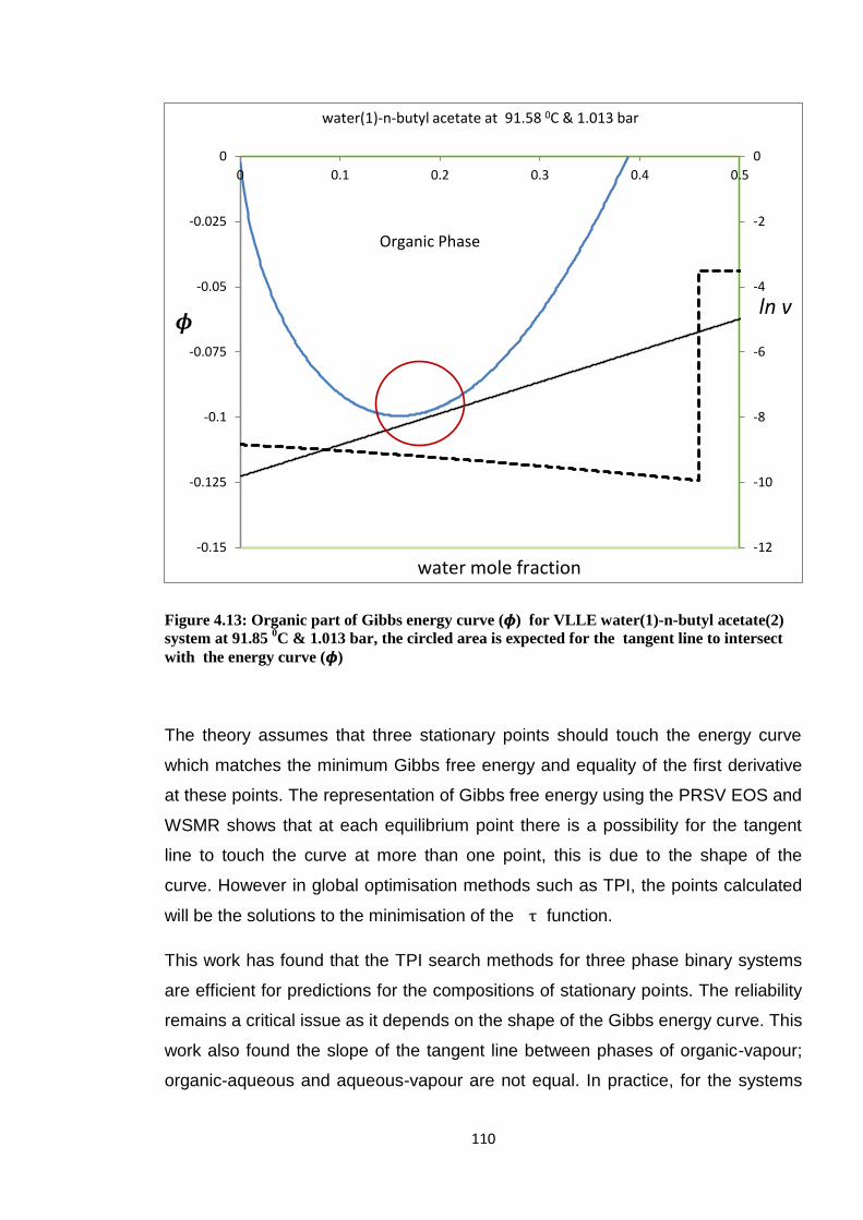
110
Figure 4.13: Organic part of Gibbs energy curve (𝝓) for VLLE water(1)-n-butyl acetate(2)
system at 91.85 0C & 1.013 bar, the circled area is expected for the tangent line to intersect
with the energy curve (𝝓)
The theory assumes that three stationary points should touch the energy curve
which matches the minimum Gibbs free energy and equality of the first derivative
at these points. The representation of Gibbs free energy using the PRSV EOS and
WSMR shows that at each equilibrium point there is a possibility for the tangent
line to touch the curve at more than one point, this is due to the shape of the
curve. However in global optimisation methods such as TPI, the points calculated
will be the solutions to the minimisation of the τ function.
This work has found that the TPI search methods for three phase binary systems
are efficient for predictions for the compositions of stationary points. The reliability
remains a critical issue as it depends on the shape of the Gibbs energy curve. This
work also found the slope of the tangent line between phases of organic-vapour;
organic-aqueous and aqueous-vapour are not equal. In practice, for the systems
-12
-10
-8
-6
-4
-2
0
-0.15
-0.125
-0.1
-0.075
-0.05
-0.025
0
0 0.1 0.2 0.3 0.4 0.5
water mole fraction
water(1)-n-butyl acetate at 91.58 0C & 1.013 bar
Organic Phase
ln v 𝝓
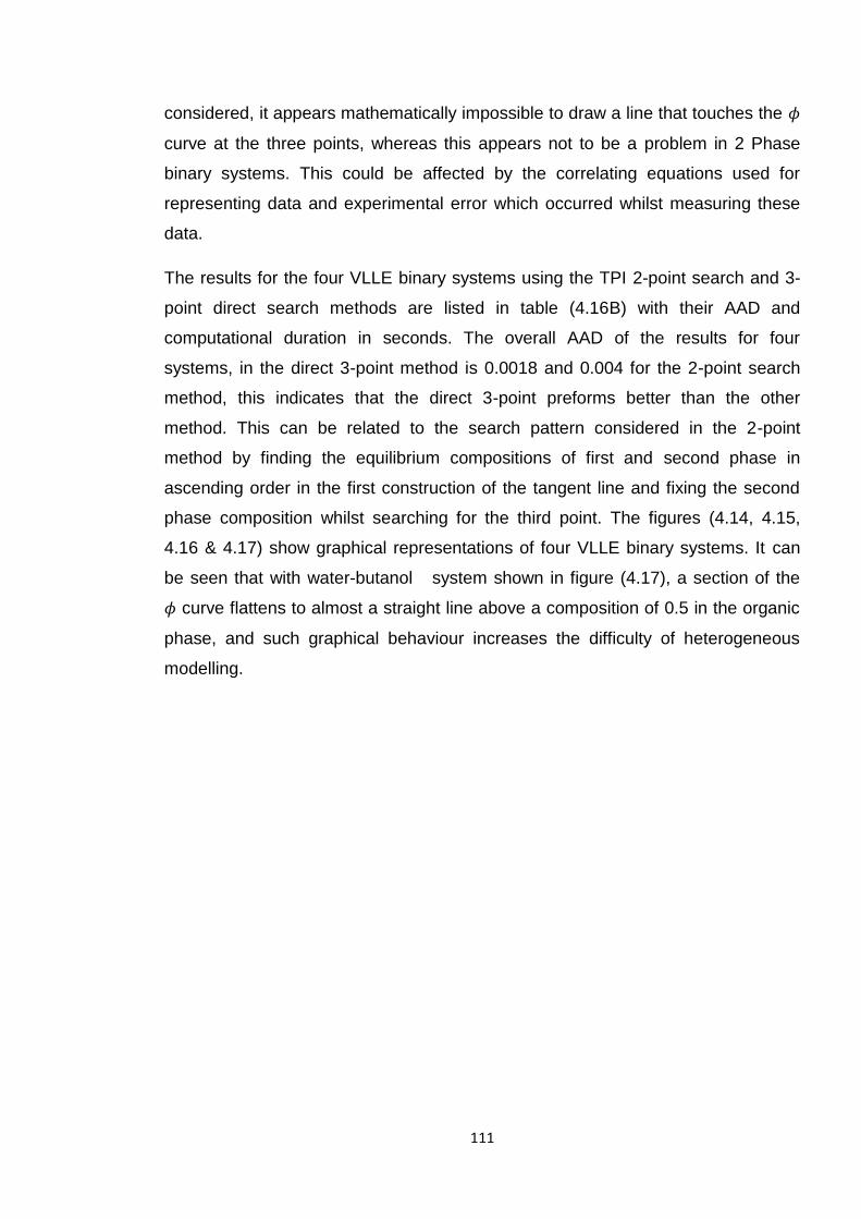
111
considered, it appears mathematically impossible to draw a line that touches the 𝜙
curve at the three points, whereas this appears not to be a problem in 2 Phase
binary systems. This could be affected by the correlating equations used for
representing data and experimental error which occurred whilst measuring these
data.
The results for the four VLLE binary systems using the TPI 2-point search and 3-
point direct search methods are listed in table (4.16B) with their AAD and
computational duration in seconds. The overall AAD of the results for four
systems, in the direct 3-point method is 0.0018 and 0.004 for the 2-point search
method, this indicates that the direct 3-point preforms better than the other
method. This can be related to the search pattern considered in the 2-point
method by finding the equilibrium compositions of first and second phase in
ascending order in the first construction of the tangent line and fixing the second
phase composition whilst searching for the third point. The figures (4.14, 4.15,
4.16 & 4.17) show graphical representations of four VLLE binary systems. It can
be seen that with water-butanol system shown in figure (4.17), a section of the
𝜙 curve flattens to almost a straight line above a composition of 0.5 in the organic
phase, and such graphical behaviour increases the difficulty of heterogeneous
modelling.
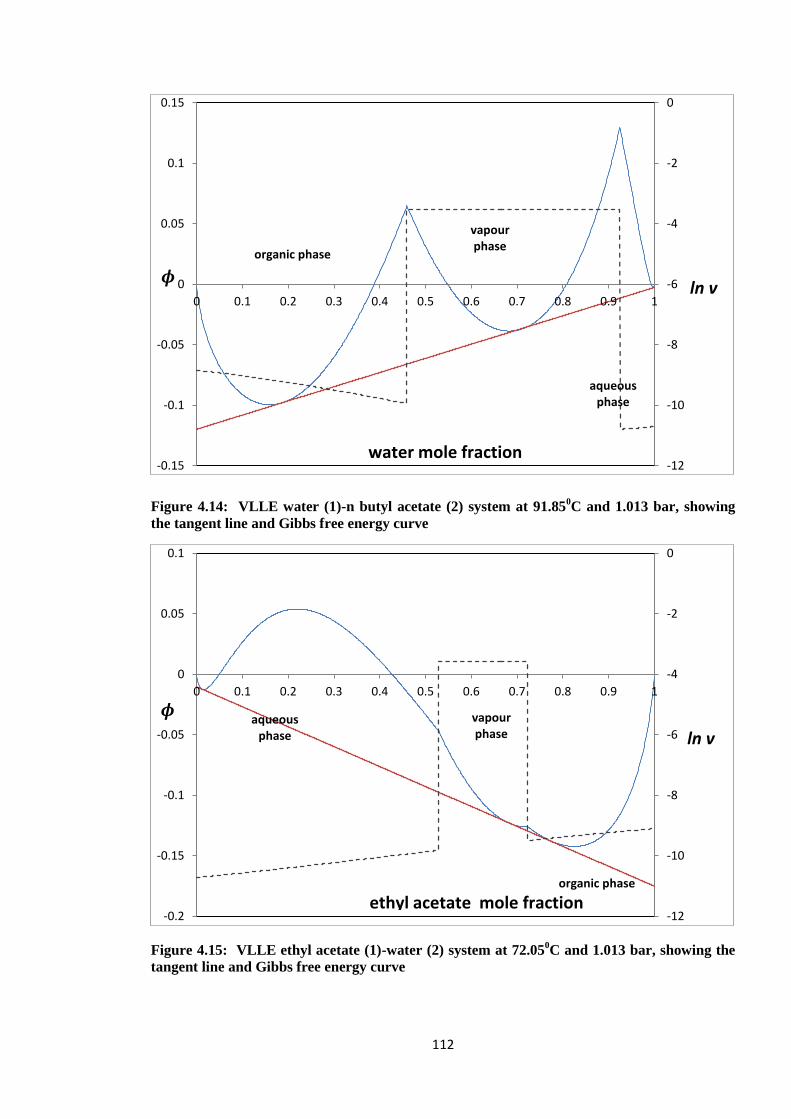
112
Figure 4.14: VLLE water (1)-n butyl acetate (2) system at 91.850C and 1.013 bar, showing
the tangent line and Gibbs free energy curve
Figure 4.15: VLLE ethyl acetate (1)-water (2) system at 72.050C and 1.013 bar, showing the
tangent line and Gibbs free energy curve
-12
-10
-8
-6
-4
-2
0
-0.15
-0.1
-0.05
0
0.05
0.1
0.15
0 0.1 0.2 0.3 0.4 0.5 0.6 0.7 0.8 0.9 1
𝝓
water mole fraction
organic phase
vapour phase
aqueous phase
ln v
-12
-10
-8
-6
-4
-2
0
-0.2
-0.15
-0.1
-0.05
0
0.05
0.1
0 0.1 0.2 0.3 0.4 0.5 0.6 0.7 0.8 0.9 1
𝝓
ethyl acetate mole fraction organic phase
vapour phase
aqueous phase ln v

113
Figure 4.16: VLLE n-butanol (1)-water (2) system at 360C and 0.068 bar, showing the tangent
line and Gibbs free energy curve
Figure 4.17: VLLE Water (1)-n-butanol (2) system at 93.770C and 1.013 bar, showing the
tangent line and Gibbs free energy curve
-12
-10
-8
-6
-4
-2
0
-0.4
-0.35
-0.3
-0.25
-0.2
-0.15
-0.1
-0.05
0
0 0.1 0.2 0.3 0.4 0.5 0.6 0.7 0.8 0.9 1
𝝓
n-butanol mole fraction
organic phase
vapour phase
aqueous phase
ln v
-12
-10
-8
-6
-4
-2
0
-0.5
-0.45
-0.4
-0.35
-0.3
-0.25
-0.2
-0.15
-0.1
-0.05
0
0 0.1 0.2 0.3 0.4 0.5 0.6 0.7 0.8 0.9 1
𝝓
water mole fraction
vapour phase
organic phase aqueous
phase
ln v
114
4.3.2 Conclusions on prediction models for LLE and VLLE binary systems
Initially this work modelled non-ideal binary systems, with and without
heterogeneous behaviour, using PRSV+WSMR; it has also demonstrated the
applicability of the Area Method and the TPI prediction method for LLE
heterogeneous systems. The two methods were tested for two binary LLE systems
in various temperatures and the results indicate that these methods are effective
for modelling such binary systems.
This work extended the TPI method to binary VLLE prediction and successfully
applied this method to four VLLE binary systems. This work has also
demonstrated the sensitivity of the TPI method to random initial values. At each
run the program produces results with slightly different solutions when compared
to the results for fixed initial values. The new method recommended for fixed initial
value depends on phase change (Cusps) compositions. The new initial scheme
was tested using the extended 2-point and 3-point direct search methods on VLLE
binary systems. The Nelder-Mead optimisation simplex was utilised in all the
minimisation processes. Due to the computational time consumption, the Area
method was only applied on the LLE systems.
This work will now investigate the applicability of the TPI method in phase
equilibrium prediction for VLLE ternary systems.

115
4.4 VLLE Ternary System Results
The correlation and predictions for four ternary VLLE systems were carried out
using data published by Younis et al. (2007). The methods used were:
1. Flash calculation
2. Tangent Plane Intersection(TPI)
3. Tangent Plane Distance Function(TPDF)
4. Systematic Initial Generator(SIG)
In the flash calculation, a feed composition (𝑧1) is calculated from the arithmetic
mean of each experimental data point using the following equation:
𝑧𝑖 = (𝑥𝑖 𝑎𝑞𝑒𝑥𝑝 + 𝑥𝑖 𝑜𝑟𝑔
𝑒𝑥𝑝 + 𝑦𝑖 𝑒𝑥𝑝)/𝑛𝑐 (4.8. 𝑎)
where 𝑛𝑐 is the number of the components and 𝑖 = 1
At equilibrium the two liquid phases are connected by a tie line and the relative
change between the two components at the overall feed compositions along a tie
line is constant:
𝐷𝑖𝑗 =𝑑𝑥𝑗
𝑑𝑥𝑖=
(𝑥𝑗 − 𝑧𝑗)
(𝑥𝑖 − 𝑧𝑖) (4.8. 𝑏)
where 𝑖 ≠ 𝑗
The second component feed composition (𝑧2) is calculated from the equation of
the tie line (4.8.b).
The VLLE flash calculation using PRSV+WSMR is explained in the theory chapter
section (3.9). The Nelder-Mead simplex was used for optimisation in the data
correlation and the estimated parameters from this correlation procedure are
shown in table (4.21) and were used in the prediction methods.
Initially the TPI method was tested on two artificial 3 phase systems of Shyu et al.
(1995), the test included various values of feed compositions inside 2 phase and 3
phase region. The results are shown in table (4.18) and (4.19) for system 1 & 2
respectively.

116
The tables below (4.22 - 4.49) show the summary of results for the flash
calculation, TPI and TPDF prediction methods for the following VLLE ternary
systems:
1. VLLE water-acetone-MEK at pressure 760 mmHg
2. VLLE water-ethanol-MEK at pressure 760 mmHg
3. VLLE water-acetone-n-butyl acetate at pressure:
3.1 360 mmHg
3.2 600 mmHg
3.3 760 mmHg
4. VLLE water- ethanol-n-butyl acetate at pressure:
4.1 360 mmHg
4.2 600 mmHg
4.3 760 mmHg
Table (4.20) shows the AAD for the flash calculations, TPDF and TPI predictions
for four systems using the PRSV+WSMR model. The simplex algorithm used for
three phase flash calculations can be found in appendix A.
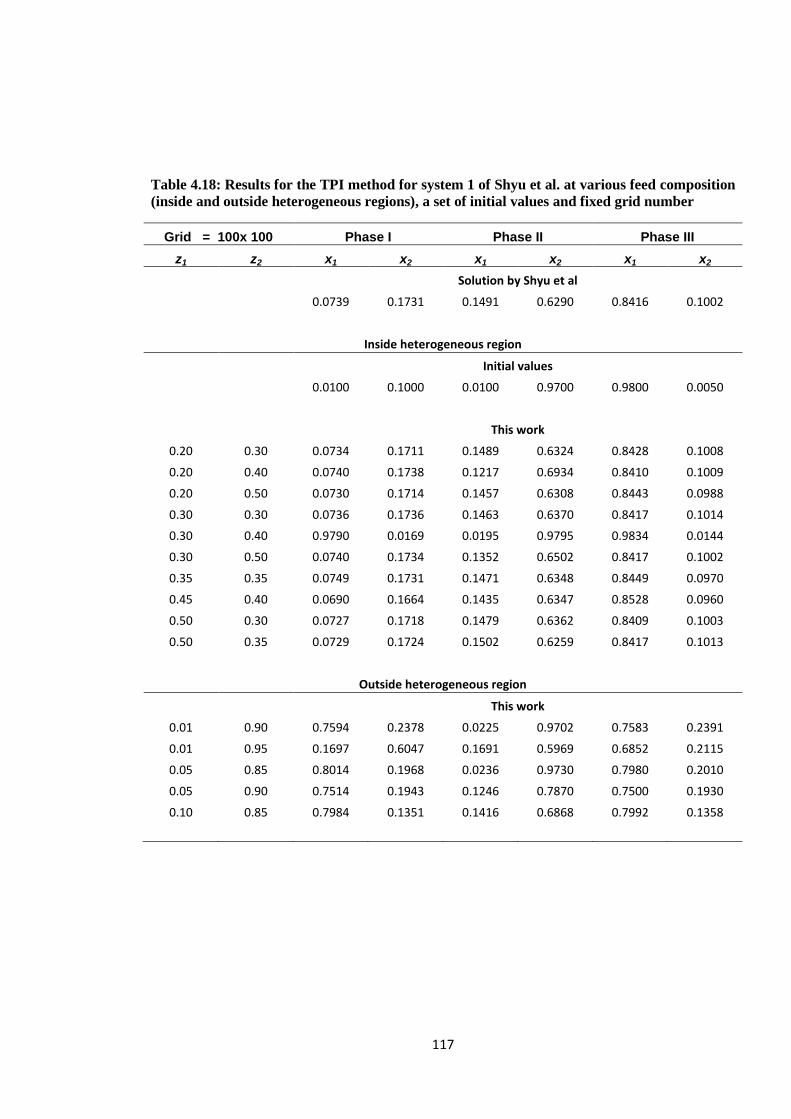
117
Table 4.18: Results for the TPI method for system 1 of Shyu et al. at various feed composition
(inside and outside heterogeneous regions), a set of initial values and fixed grid number
Grid = 100x 100 Phase I Phase II Phase III
z1 z2 x1 x2 x1 x2 x1 x2
Solution by Shyu et al
0.0739 0.1731 0.1491 0.6290 0.8416 0.1002
Inside heterogeneous region
Initial values
0.0100 0.1000 0.0100 0.9700 0.9800 0.0050
This work
0.20 0.30 0.0734 0.1711 0.1489 0.6324 0.8428 0.1008
0.20 0.40 0.0740 0.1738 0.1217 0.6934 0.8410 0.1009
0.20 0.50 0.0730 0.1714 0.1457 0.6308 0.8443 0.0988
0.30 0.30 0.0736 0.1736 0.1463 0.6370 0.8417 0.1014
0.30 0.40 0.9790 0.0169 0.0195 0.9795 0.9834 0.0144
0.30 0.50 0.0740 0.1734 0.1352 0.6502 0.8417 0.1002
0.35 0.35 0.0749 0.1731 0.1471 0.6348 0.8449 0.0970
0.45 0.40 0.0690 0.1664 0.1435 0.6347 0.8528 0.0960
0.50 0.30 0.0727 0.1718 0.1479 0.6362 0.8409 0.1003
0.50 0.35 0.0729 0.1724 0.1502 0.6259 0.8417 0.1013
Outside heterogeneous region
This work
0.01 0.90 0.7594 0.2378 0.0225 0.9702 0.7583 0.2391
0.01 0.95 0.1697 0.6047 0.1691 0.5969 0.6852 0.2115
0.05 0.85 0.8014 0.1968 0.0236 0.9730 0.7980 0.2010
0.05 0.90 0.7514 0.1943 0.1246 0.7870 0.7500 0.1930
0.10 0.85 0.7984 0.1351 0.1416 0.6868 0.7992 0.1358
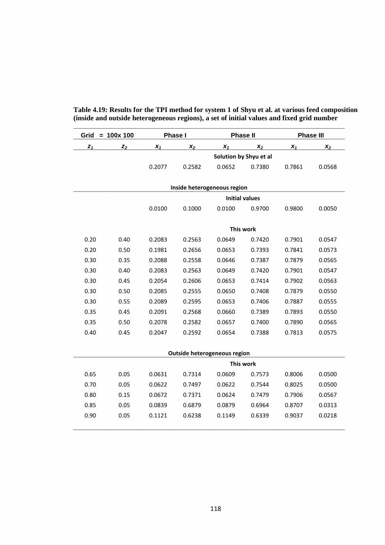
118
Table 4.19: Results for the TPI method for system 1 of Shyu et al. at various feed composition
(inside and outside heterogeneous regions), a set of initial values and fixed grid number
Grid = 100x 100 Phase I Phase II Phase III
z1 z2 x1 x2 x1 x2 x1 x2
Solution by Shyu et al
0.2077 0.2582 0.0652 0.7380 0.7861 0.0568
Inside heterogeneous region
Initial values
0.0100 0.1000 0.0100 0.9700 0.9800 0.0050
This work
0.20 0.40 0.2083 0.2563 0.0649 0.7420 0.7901 0.0547
0.20 0.50 0.1981 0.2656 0.0653 0.7393 0.7841 0.0573
0.30 0.35 0.2088 0.2558 0.0646 0.7387 0.7879 0.0565
0.30 0.40 0.2083 0.2563 0.0649 0.7420 0.7901 0.0547
0.30 0.45 0.2054 0.2606 0.0653 0.7414 0.7902 0.0563
0.30 0.50 0.2085 0.2555 0.0650 0.7408 0.7879 0.0550
0.30 0.55 0.2089 0.2595 0.0653 0.7406 0.7887 0.0555
0.35 0.45 0.2091 0.2568 0.0660 0.7389 0.7893 0.0550
0.35 0.50 0.2078 0.2582 0.0657 0.7400 0.7890 0.0565
0.40 0.45 0.2047 0.2592 0.0654 0.7388 0.7813 0.0575
Outside heterogeneous region
This work
0.65 0.05 0.0631 0.7314 0.0609 0.7573 0.8006 0.0500
0.70 0.05 0.0622 0.7497 0.0622 0.7544 0.8025 0.0500
0.80 0.15 0.0672 0.7371 0.0624 0.7479 0.7906 0.0567
0.85 0.05 0.0839 0.6879 0.0879 0.6964 0.8707 0.0313
0.90 0.05 0.1121 0.6238 0.1149 0.6339 0.9037 0.0218
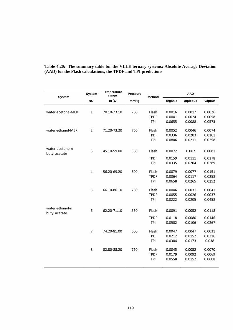
119
Table 4.20: The summary table for the VLLE ternary systems: Absolute Average Deviation
(AAD) for the Flash calculations, the TPDF and TPI predictions
System System
Temperature range
Pressure Method
AAD
NO. In 0C mmHg organic aqueous vapour
water-acetone-MEK 1 70.10-73.10 760 Flash 0.0016 0.0017 0.0026
TPDF 0.0041 0.0024 0.0058
TPI 0.0655 0.0088 0.0573
water-ethanol-MEK 2 71.20-73.20 760 Flash 0.0052 0.0046 0.0074
TPDF 0.0336 0.0203 0.0161
TPI 0.0806 0.0211 0.0258
water-acetone-n butyl acetate
3 45.10-59.00 360 Flash 0.0072 0.007 0.0081
TPDF 0.0159 0.0111 0.0178
TPI 0.0335 0.0204 0.0289
4 56.20-69.20 600 Flash 0.0079 0.0077 0.0151
TPDF 0.0064 0.0117 0.0258
TPI 0.0658 0.0265 0.0252
5 66.10-86.10 760 Flash 0.0046 0.0031 0.0041
TPDF 0.0055 0.0026 0.0037
TPI 0.0222 0.0205 0.0458
water-ethanol-n butyl acetate
6 62.20-71.10 360 Flash 0.0091 0.0052 0.0118
TPDF 0.0118 0.0080 0.0146
TPI 0.0502 0.0106 0.0267
7 74.20-81.00 600 Flash 0.0047 0.0047 0.0031
TPDF 0.0212 0.0152 0.0216
TPI 0.0304 0.0173 0.038
8 82.80-88.20 760 Flash 0.0045 0.0052 0.0070
TPDF 0.0179 0.0092 0.0069
TPI 0.0558 0.0152 0.0608
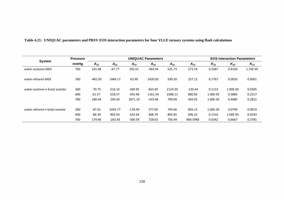
120
Table 4.21: UNIQUAC parameters and PRSV EOS interaction parameters for four VLLE ternary systems using flash calculations
System Pressure UNIQUAC Parameters EOS interaction Parameters
mmHg A12 A21 A23 A32 A31 A13 K12 K23 K13
water-acetone-MEK 760 101.48 -67.77 292.61 -364.94 525.73 273.54 0.5587 0.9150 1.74E-05
water-ethanol-MEK 760 -481.95 1484.17 63.99 2420.92 599.20 257.12 0.7767 0.0033 0.0001
water-acetone-n butyl acetate 360 -70.75 616.16 -269.95 663.49 2124.50 -120.44 0.1114 1.00E-05 0.9305
600 61.57 618.57 -355.96 1161.59 2588.11 800.82 1.00E-05 0.3883 0.2317
760 180.44 294.50 1871.19 -419.96 799.09 404.92 1.00E-05 0.4085 0.2831
water-ethanol-n butyl acetate 360 -87.01 3443.77 -178.49 377.69 794.66 856.13 1.00E-05 0.0799 0.0019
600 -86.30 802.03 -102.64 468.79 895.85 696.22 0.1310 1.00E-05 0.0243
760 179.96 -263.45 -300.59 728.63 756.49 469.5948 0.6342 0.6667 0.3781

121
4.4.1 VLLE system: water (1)-acetone (2)-MEK (3) at pressure 760 mmHg
Table 4.22: VLLE ternary system water (1)-acetone (2)-methyl ethyl ketone (3) at 760 mmHg, flash calculation, TPDF & TPI predictions Temperature Experimental Flash calculation TPDF Prediction TPI Prediction
in C water acetone MEK
water acetone MEK
water acetone MEK
water acetone MEK
Organic Phase
73.10 0.450 0.016 0.534
0.445 0.017 0.539
0.444 0.015 0.542
0.432 0.005 0.563 72.60 0.451 0.032 0.518
0.451 0.030 0.519
0.452 0.028 0.520
0.440 0.011 0.549
72.20 0.465 0.044 0.490
0.466 0.043 0.491
0.473 0.042 0.485
0.470 0.025 0.505 71.80 0.502 0.066 0.432
0.506 0.063 0.431
0.510 0.065 0.425
0.504 0.046 0.450
71.30 0.549 0.085 0.366
0.550 0.083 0.367
0.559 0.085 0.356
0.517 0.055 0.429 70.90 0.578 0.093 0.330
0.578 0.091 0.331
0.573 0.094 0.333
0.618 0.059 0.323
70.30 0.613 0.096 0.291
0.611 0.097 0.292
0.609 0.095 0.296
0.620 0.070 0.310 70.10 0.684 0.089 0.227
0.683 0.092 0.225
0.682 0.090 0.229
0.721 0.083 0.197
Aqueous Phase 73.10 0.947 0.003 0.049
0.954 0.002 0.044
0.950 0.003 0.047
0.967 0.009 0.024
72.60 0.948 0.006 0.046
0.950 0.005 0.045
0.951 0.006 0.043
0.961 0.014 0.025 72.20 0.939 0.010 0.051
0.942 0.008 0.050
0.943 0.009 0.048
0.948 0.020 0.033
71.80 0.926 0.017 0.056
0.928 0.015 0.057
0.929 0.016 0.054
0.935 0.022 0.043 71.30 0.907 0.027 0.066
0.908 0.025 0.066
0.908 0.027 0.065
0.908 0.027 0.065
70.90 0.896 0.033 0.071
0.897 0.031 0.072
0.892 0.034 0.074
0.896 0.037 0.067 70.30 0.876 0.041 0.083
0.877 0.040 0.083
0.881 0.039 0.080
0.875 0.041 0.083
70.10 0.823 0.059 0.118
0.825 0.059 0.117
0.817 0.061 0.122
0.824 0.059 0.117
Vapour Phase 73.10 0.352 0.031 0.617
0.351 0.032 0.618
0.346 0.034 0.620
0.272 0.026 0.702
72.60 0.351 0.060 0.590
0.344 0.060 0.596
0.341 0.060 0.598
0.263 0.047 0.689 72.20 0.343 0.087 0.569
0.337 0.087 0.576
0.331 0.095 0.573
0.287 0.094 0.619
71.80 0.338 0.135 0.527
0.328 0.135 0.537
0.323 0.133 0.544
0.278 0.131 0.591 71.30 0.314 0.186 0.500
0.315 0.187 0.499
0.312 0.190 0.499
0.279 0.161 0.560
70.90 0.311 0.209 0.480
0.311 0.209 0.480
0.306 0.214 0.480
0.294 0.181 0.525 70.30 0.305 0.231 0.464
0.307 0.231 0.462
0.300 0.229 0.471
0.299 0.234 0.468
70.10 0.304 0.250 0.446
0.307 0.246 0.447
0.294 0.251 0.455
0.295 0.250 0.455
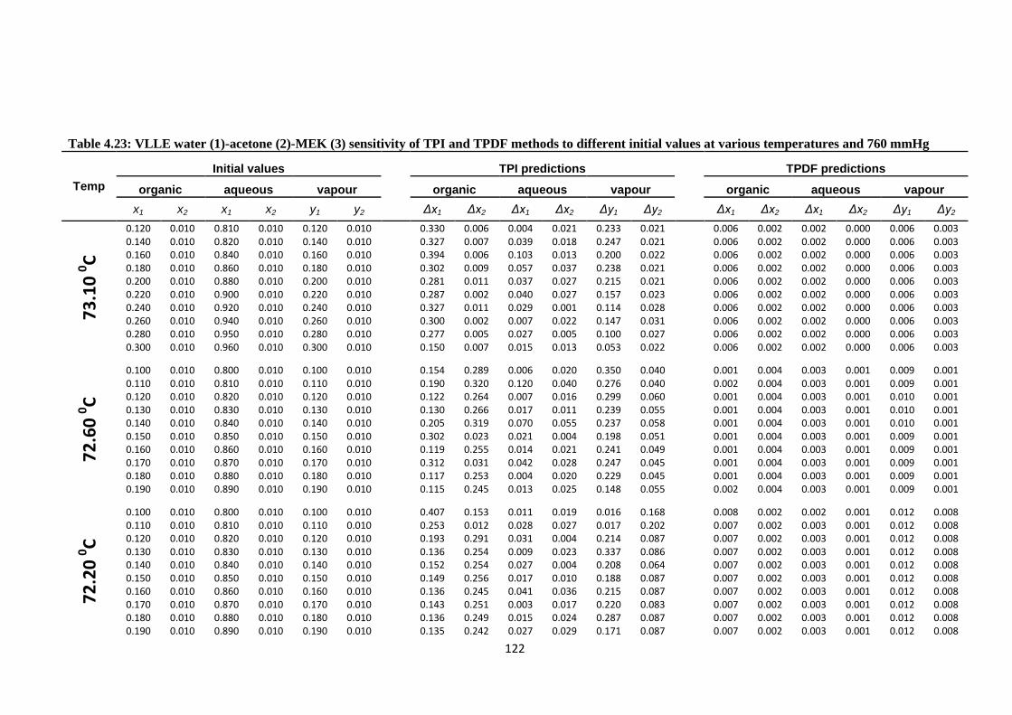
122
Table 4.23: VLLE water (1)-acetone (2)-MEK (3) sensitivity of TPI and TPDF methods to different initial values at various temperatures and 760 mmHg
Temp
Initial values TPI predictions TPDF predictions
organic aqueous vapour
organic aqueous vapour
organic aqueous vapour
x1 x2 x1 x2 y1 y2 Δx1 Δx2 Δx1 Δx2 Δy1 Δy2 Δx1 Δx2 Δx1 Δx2 Δy1 Δy2
73
.10
0C
0.120 0.010 0.810 0.010 0.120 0.010
0.330 0.006 0.004 0.021 0.233 0.021
0.006 0.002 0.002 0.000 0.006 0.003
0.140 0.010 0.820 0.010 0.140 0.010
0.327 0.007 0.039 0.018 0.247 0.021
0.006 0.002 0.002 0.000 0.006 0.003
0.160 0.010 0.840 0.010 0.160 0.010
0.394 0.006 0.103 0.013 0.200 0.022
0.006 0.002 0.002 0.000 0.006 0.003
0.180 0.010 0.860 0.010 0.180 0.010
0.302 0.009 0.057 0.037 0.238 0.021
0.006 0.002 0.002 0.000 0.006 0.003
0.200 0.010 0.880 0.010 0.200 0.010
0.281 0.011 0.037 0.027 0.215 0.021
0.006 0.002 0.002 0.000 0.006 0.003
0.220 0.010 0.900 0.010 0.220 0.010
0.287 0.002 0.040 0.027 0.157 0.023
0.006 0.002 0.002 0.000 0.006 0.003
0.240 0.010 0.920 0.010 0.240 0.010
0.327 0.011 0.029 0.001 0.114 0.028
0.006 0.002 0.002 0.000 0.006 0.003
0.260 0.010 0.940 0.010 0.260 0.010
0.300 0.002 0.007 0.022 0.147 0.031
0.006 0.002 0.002 0.000 0.006 0.003
0.280 0.010 0.950 0.010 0.280 0.010
0.277 0.005 0.027 0.005 0.100 0.027
0.006 0.002 0.002 0.000 0.006 0.003
0.300 0.010 0.960 0.010 0.300 0.010
0.150 0.007 0.015 0.013 0.053 0.022
0.006 0.002 0.002 0.000 0.006 0.003
72
.60
0C
0.100 0.010 0.800 0.010 0.100 0.010
0.154 0.289 0.006 0.020 0.350 0.040
0.001 0.004 0.003 0.001 0.009 0.001 0.110 0.010 0.810 0.010 0.110 0.010
0.190 0.320 0.120 0.040 0.276 0.040
0.002 0.004 0.003 0.001 0.009 0.001
0.120 0.010 0.820 0.010 0.120 0.010
0.122 0.264 0.007 0.016 0.299 0.060
0.001 0.004 0.003 0.001 0.010 0.001 0.130 0.010 0.830 0.010 0.130 0.010
0.130 0.266 0.017 0.011 0.239 0.055
0.001 0.004 0.003 0.001 0.010 0.001
0.140 0.010 0.840 0.010 0.140 0.010
0.205 0.319 0.070 0.055 0.237 0.058
0.001 0.004 0.003 0.001 0.010 0.001 0.150 0.010 0.850 0.010 0.150 0.010
0.302 0.023 0.021 0.004 0.198 0.051
0.001 0.004 0.003 0.001 0.009 0.001
0.160 0.010 0.860 0.010 0.160 0.010
0.119 0.255 0.014 0.021 0.241 0.049
0.001 0.004 0.003 0.001 0.009 0.001 0.170 0.010 0.870 0.010 0.170 0.010
0.312 0.031 0.042 0.028 0.247 0.045
0.001 0.004 0.003 0.001 0.009 0.001
0.180 0.010 0.880 0.010 0.180 0.010
0.117 0.253 0.004 0.020 0.229 0.045
0.001 0.004 0.003 0.001 0.009 0.001 0.190 0.010 0.890 0.010 0.190 0.010
0.115 0.245 0.013 0.025 0.148 0.055
0.002 0.004 0.003 0.001 0.009 0.001
72
.20
0C
0.100 0.010 0.800 0.010 0.100 0.010
0.407 0.153 0.011 0.019 0.016 0.168
0.008 0.002 0.002 0.001 0.012 0.008 0.110 0.010 0.810 0.010 0.110 0.010
0.253 0.012 0.028 0.027 0.017 0.202
0.007 0.002 0.003 0.001 0.012 0.008
0.120 0.010 0.820 0.010 0.120 0.010
0.193 0.291 0.031 0.004 0.214 0.087
0.007 0.002 0.003 0.001 0.012 0.008 0.130 0.010 0.830 0.010 0.130 0.010
0.136 0.254 0.009 0.023 0.337 0.086
0.007 0.002 0.003 0.001 0.012 0.008
0.140 0.010 0.840 0.010 0.140 0.010
0.152 0.254 0.027 0.004 0.208 0.064
0.007 0.002 0.003 0.001 0.012 0.008 0.150 0.010 0.850 0.010 0.150 0.010
0.149 0.256 0.017 0.010 0.188 0.087
0.007 0.002 0.003 0.001 0.012 0.008
0.160 0.010 0.860 0.010 0.160 0.010
0.136 0.245 0.041 0.036 0.215 0.087
0.007 0.002 0.003 0.001 0.012 0.008 0.170 0.010 0.870 0.010 0.170 0.010
0.143 0.251 0.003 0.017 0.220 0.083
0.007 0.002 0.003 0.001 0.012 0.008
0.180 0.010 0.880 0.010 0.180 0.010
0.136 0.249 0.015 0.024 0.287 0.087
0.007 0.002 0.003 0.001 0.012 0.008 0.190 0.010 0.890 0.010 0.190 0.010
0.135 0.242 0.027 0.029 0.171 0.087
0.007 0.002 0.003 0.001 0.012 0.008
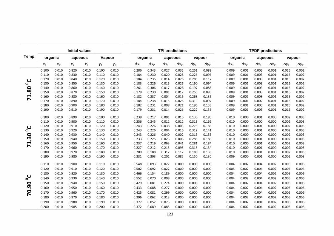
123
Temp
Initial values TPI predictions TPDF predictions
organic aqueous Vapour
organic aqueous vapour
organic aqueous vapour
x1 x2 x1 x2 y1 y2 Δx1 Δx2 Δx1 Δx2 Δy1 Δy2 Δx1 Δx2 Δx1 Δx2 Δy1 Δy2
71
.80
0C
0.100 0.010 0.820 0.010 0.100 0.010
0.286 0.343 0.027 0.035 0.251 0.089
0.009 0.001 0.003 0.001 0.015 0.002 0.110 0.010 0.830 0.010 0.110 0.010
0.184 0.230 0.020 0.028 0.225 0.096
0.009 0.001 0.003 0.001 0.015 0.002
0.120 0.010 0.840 0.010 0.120 0.010
0.184 0.235 0.014 0.026 0.285 0.117
0.009 0.001 0.003 0.001 0.015 0.002 0.130 0.010 0.850 0.010 0.130 0.010
0.183 0.226 0.015 0.025 0.190 0.094
0.009 0.001 0.003 0.001 0.016 0.002
0.140 0.010 0.860 0.010 0.140 0.010
0.261 0.306 0.017 0.028 0.197 0.088
0.009 0.001 0.003 0.001 0.015 0.002 0.150 0.010 0.870 0.010 0.150 0.010
0.179 0.230 0.001 0.017 0.255 0.095
0.008 0.001 0.003 0.001 0.016 0.002
0.160 0.010 0.880 0.010 0.160 0.010
0.182 0.237 0.004 0.016 0.263 0.135
0.009 0.001 0.003 0.001 0.015 0.002 0.170 0.010 0.890 0.010 0.170 0.010
0.184 0.238 0.015 0.026 0.319 0.097
0.009 0.001 0.002 0.001 0.015 0.002
0.180 0.010 0.900 0.010 0.180 0.010
0.182 0.231 0.008 0.021 0.196 0.133
0.009 0.001 0.003 0.001 0.015 0.002 0.190 0.010 0.910 0.010 0.190 0.010
0.179 0.231 0.014 0.026 0.222 0.135
0.009 0.001 0.003 0.001 0.015 0.002
71
.30
0C
0.100 0.010 0.890 0.010 0.100 0.010
0.239 0.217 0.001 0.016 0.130 0.185
0.010 0.000 0.001 0.000 0.002 0.003 0.110 0.010 0.900 0.010 0.110 0.010
0.256 0.245 0.011 0.012 0.313 0.166
0.010 0.000 0.000 0.000 0.002 0.003
0.120 0.010 0.910 0.010 0.120 0.010
0.243 0.226 0.038 0.003 0.275 0.186
0.010 0.000 0.001 0.000 0.002 0.003 0.130 0.010 0.920 0.010 0.130 0.010
0.243 0.226 0.004 0.016 0.312 0.141
0.010 0.000 0.001 0.000 0.002 0.003
0.140 0.010 0.930 0.010 0.140 0.010
0.243 0.226 0.040 0.002 0.313 0.153
0.010 0.000 0.000 0.000 0.002 0.003 0.150 0.010 0.940 0.010 0.150 0.010
0.233 0.225 0.023 0.006 0.285 0.185
0.010 0.000 0.001 0.000 0.002 0.003
0.160 0.010 0.950 0.010 0.160 0.010
0.237 0.219 0.063 0.041 0.281 0.184
0.010 0.000 0.001 0.000 0.002 0.003 0.170 0.010 0.960 0.010 0.170 0.010
0.227 0.212 0.213 0.093 0.313 0.134
0.010 0.000 0.001 0.000 0.002 0.003
0.180 0.010 0.970 0.010 0.180 0.010
0.209 0.188 0.312 0.112 0.180 0.138
0.010 0.000 0.001 0.000 0.002 0.003 0.190 0.010 0.980 0.010 0.190 0.010
0.331 0.303 0.201 0.085 0.150 0.130
0.009 0.000 0.001 0.000 0.002 0.003
70
.90
0C
0.110 0.010 0.900 0.010 0.110 0.010
0.548 0.093 0.027 0.000 0.000 0.000
0.004 0.002 0.004 0.002 0.005 0.006
0.120 0.010 0.910 0.010 0.120 0.010
0.502 0.092 0.022 0.000 0.000 0.000
0.005 0.002 0.004 0.002 0.005 0.006
0.130 0.010 0.920 0.010 0.130 0.010
0.466 0.154 0.189 0.000 0.000 0.000
0.004 0.002 0.004 0.002 0.005 0.006
0.140 0.010 0.930 0.010 0.140 0.010
0.552 0.070 0.008 0.000 0.000 0.000
0.004 0.002 0.004 0.002 0.005 0.006
0.150 0.010 0.940 0.010 0.150 0.010
0.429 0.081 0.274 0.000 0.000 0.000
0.004 0.002 0.004 0.002 0.005 0.006
0.160 0.010 0.950 0.010 0.160 0.010
0.433 0.088 0.277 0.000 0.000 0.000
0.004 0.002 0.004 0.002 0.005 0.006
0.170 0.010 0.960 0.010 0.170 0.010
0.425 0.081 0.299 0.000 0.000 0.000
0.004 0.002 0.004 0.002 0.005 0.006
0.180 0.010 0.970 0.010 0.180 0.010
0.396 0.062 0.313 0.000 0.000 0.000
0.004 0.002 0.004 0.002 0.005 0.006
0.190 0.010 0.980 0.010 0.190 0.010
0.377 0.052 0.073 0.000 0.000 0.000
0.004 0.002 0.004 0.002 0.005 0.006
0.200 0.010 0.985 0.010 0.200 0.010 0.372 0.089 0.085 0.000 0.000 0.000 0.004 0.002 0.004 0.002 0.005 0.006

124
Table 4.24: The SIG, TPI and TPDF results on VLLE ternary system of water (1)-acetone (2)MEK (3) at 760 mm Hg, different sets of feed composition were
chosen outside heterogeneous region with various temperatures
z1 z2 T in 0C Method
Phase I Phase II Phase III No Phases
x1 x2 x1 x2 y1 y2
0.500 0.300 73.10 SIG 0.9490 0.0317 0.9490 0.0316 0.3400 0.3960 2 TPI 0.0207 0.0001 0.9483 0.0237 0.3314 0.3020 3
TPDF 0.9490 0.0316 0.9490 0.0316 0.3400 0.3956 2
0.600 0.300 72.60
SIG 0.9482 0.0392 0.9483 0.0392 0.3314 0.5021 2 TPI 0.0035 0.0658 0.9555 0.0221 0.3166 0.3002 3
TPDF 0.9483 0.0391 0.9483 0.0391 0.3314 0.5012 2
0.700 0.200 72.20
SIG 0.9440 0.0379 0.9444 0.0377 0.3260 0.4502 2 TPI 0.5331 0.0243 0.9445 0.0184 0.0233 0.2222 3
TPDF 0.9445 0.0376 0.9445 0.0376 0.3261 0.4484 2
0.300 0.500 71.80
SIG 0.9271 0.0517 0.9271 0.0517 0.3177 0.5339 2 TPI 0.4694 0.4525 0.9269 0.0678 0.2462 0.6234 3
TPDF 0.9271 0.0517 0.9271 0.0517 0.2984 0.5012 2
0.200 0.700 71.30
SIG 0.4012 0.5174 0.4012 0.5174 0.1903 0.6677 2 TPI 0.3077 0.4136 0.3504 0.6359 0.1233 0.7003 3
TPDF 0.4012 0.5174 0.4012 0.5174 0.1996 0.7004 2
0.250 0.650 70.90
SIG 0.8570 0.1185 0.8570 0.1185 0.2574 0.6743 2 TPI 0.4077 0.5865 0.9362 0.0413 0.1494 0.6905 3
TPDF 0.8570 0.1185 0.8570 0.1185 0.2486 0.6512 2
0.100 0.650 70.30
SIG 0.1869 0.5843 0.1869 0.5844 0.1247 0.8120 2 TPI 0.0030 0.6004 0.1949 0.5966 0.3096 0.6707 3
TPDF 0.1868 0.5844 0.1868 0.5844 0.0998 0.6501 2
0.150 0.750 70.10
SIG 0.2720 0.6412 0.2720 0.6412 0.1415 0.7090 2 TPI 0.2697 0.4095 0.2697 0.7280 0.1008 0.7504 3
TPDF 0.2720 0.6412 0.2720 0.6412 0.1497 0.7502 2
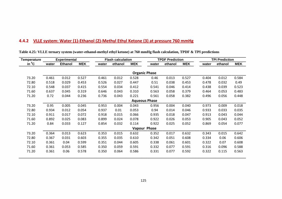
125
4.4.2 VLLE system: Water (1)-Ethanol (2)-Methyl Ethyl Ketone (3) at pressure 760 mmHg
Table 4.25: VLLE ternary system (water-ethanol-methyl ethyl ketone) at 760 mmHg flash calculation, TPDF & TPI predictions
Temperature Experimental Flash calculation TPDF Prediction TPI Prediction
in 0C water Ethanol MEK
water ethanol MEK
water ethanol MEK
water ethanol MEK
Organic Phase
73.20 0.461 0.012 0.527
0.461 0.012 0.528
0.46 0.013 0.527
0.404 0.012 0.584 72.80 0.518 0.029 0.453
0.526 0.027 0.447
0.51 0.038 0.453
0.478 0.032 0.49
72.10 0.548 0.037 0.415
0.554 0.034 0.412
0.541 0.046 0.414
0.438 0.039 0.523 71.60 0.637 0.045 0.319
0.646 0.043 0.310
0.563 0.058 0.379
0.464 0.053 0.483
71.20 0.72 0.044 0.236
0.736 0.043 0.221
0.561 0.058 0.382
0.496 0.056 0.448
Aqueous Phase
73.20 0.95 0.005 0.045
0.953 0.004 0.043
0.956 0.004 0.040
0.973 0.009 0.018 72.80 0.934 0.012 0.054
0.937 0.01 0.053
0.94 0.014 0.046
0.933 0.033 0.035
72.10 0.911 0.017 0.072
0.918 0.015 0.066
0.935 0.018 0.047
0.913 0.043 0.044 71.60 0.892 0.025 0.083
0.899 0.024 0.078
0.922 0.026 0.053
0.905 0.043 0.052
71.20 0.84 0.033 0.127
0.854 0.032 0.114
0.922 0.025 0.052
0.869 0.054 0.077
Vapour Phase
73.20 0.364 0.013 0.623
0.353 0.015 0.632
0.352 0.017 0.632
0.343 0.015 0.642 72.80 0.367 0.031 0.603
0.355 0.035 0.610
0.342 0.051 0.608
0.334 0.06 0.606
72.10 0.361 0.04 0.599
0.351 0.044 0.605
0.338 0.061 0.601
0.322 0.07 0.608 71.60 0.361 0.053 0.585
0.350 0.059 0.591
0.332 0.077 0.591
0.316 0.096 0.588
71.20 0.361 0.06 0.578
0.350 0.064 0.586
0.331 0.077 0.592
0.322 0.115 0.563

126
Table 4.26: VLLE water (1)-ethanol (2)-MEK (3) sensitivity of TPI and TPDF methods to different initial values at temperatures; 73.2, 72.8 & 72.10C,
pressure 760 mmHg
Temp
Initial values TPI predictions TPDF predictions
organic aqueous vapour
organic aqueous vapour
organic aqueous vapour
x1 x2 x1 x2 y1 y2 Δx1 Δx2 Δx1 Δx2 Δy1 Δy2 Δx1 Δx2 Δx1 Δx2 Δy1 Δy2
73
.20
0C
0.010 0.01 0.725 0.01 0.050 0.01
0.376 0.205 0.257 0.221 0.064 0.267
0.001 0.000 0.007 0.001 0.012 0.004
0.025 0.01 0.750 0.01 0.075 0.01
0.318 0.205 0.238 0.153 0.321 0.251
0.001 0.000 0.007 0.001 0.012 0.004
0.050 0.01 0.775 0.01 0.100 0.01
0.407 0.002 0.152 0.144 0.268 0.011
0.001 0.000 0.007 0.001 0.012 0.004
0.075 0.01 0.800 0.01 0.125 0.01
0.398 0.016 0.172 0.159 0.229 0.009
0.001 0.000 0.007 0.001 0.012 0.004
0.100 0.01 0.825 0.01 0.150 0.01
0.361 0.010 0.170 0.142 0.221 0.004
0.001 0.000 0.007 0.001 0.012 0.004
0.125 0.01 0.850 0.01 0.175 0.01
0.336 0.003 0.214 0.195 0.220 0.008
0.001 0.000 0.007 0.001 0.012 0.004
0.150 0.01 0.875 0.01 0.200 0.01
0.320 0.013 0.228 0.209 0.194 0.005
0.001 0.000 0.007 0.001 0.012 0.004
0.175 0.01 0.900 0.01 0.225 0.01
0.277 0.008 0.050 0.005 0.139 0.003
0.001 0.000 0.007 0.001 0.012 0.004
0.200 0.01 0.925 0.01 0.250 0.01
0.298 0.007 0.025 0.005 0.114 0.003
0.001 0.000 0.007 0.001 0.012 0.004
0.225 0.01 0.950 0.01 0.275 0.01
0.443 0.002 0.000 0.022 0.292 0.006
0.001 0.000 0.007 0.001 0.012 0.004
72
.80
0C
0.010 0.01 0.800 0.01 0.050 0.01
0.480 0.125 0.322 0.309 0.094 0.311
0.009 0.009 0.007 0.002 0.025 0.019
0.025 0.01 0.820 0.01 0.075 0.01
0.316 0.029 0.302 0.282 0.127 0.316
0.009 0.009 0.007 0.002 0.025 0.019
0.050 0.01 0.840 0.01 0.100 0.01
0.450 0.212 0.269 0.238 0.079 0.266
0.009 0.009 0.007 0.002 0.025 0.02
0.075 0.01 0.860 0.01 0.125 0.01
0.444 0.008 0.248 0.237 0.268 0.016
0.009 0.009 0.007 0.002 0.025 0.019
0.100 0.01 0.880 0.01 0.150 0.01
0.421 0.016 0.284 0.269 0.251 0.014
0.009 0.009 0.007 0.002 0.025 0.019
0.125 0.01 0.900 0.01 0.175 0.01
0.395 0.016 0.302 0.288 0.224 0.021
0.009 0.009 0.007 0.002 0.025 0.02
0.150 0.01 0.920 0.01 0.200 0.01
0.370 0.007 0.314 0.306 0.196 0.022
0.009 0.009 0.007 0.002 0.025 0.02
0.175 0.01 0.940 0.01 0.225 0.01
0.354 0.003 0.295 0.276 0.185 0.026
0.009 0.009 0.007 0.002 0.025 0.02
0.200 0.01 0.960 0.01 0.250 0.01
0.319 0.020 0.351 0.341 0.129 0.029
0.009 0.009 0.007 0.002 0.025 0.02
0.225 0.01 0.980 0.01 0.275 0.01
0.349 0.068 0.275 0.248 0.128 0.010
0.009 0.009 0.007 0.002 0.025 0.02
72
.10
0C
0.195 0.01 0.800 0.01 0.100 0.01
0.237 0.263 0.156 0.170 0.292 0.037
0.008 0.009 0.023 0.001 0.023 0.021
0.198 0.01 0.820 0.01 0.125 0.01
0.274 0.266 0.274 0.244 0.089 0.001
0.008 0.009 0.024 0.001 0.024 0.021
0.201 0.01 0.840 0.01 0.150 0.01
0.279 0.274 0.286 0.267 0.115 0.016
0.007 0.009 0.023 0.001 0.024 0.021
0.204 0.01 0.860 0.01 0.175 0.01
0.295 0.287 0.276 0.256 0.125 0.004
0.008 0.009 0.024 0.001 0.023 0.021
0.207 0.01 0.880 0.01 0.200 0.01
0.261 0.263 0.057 0.104 0.146 0.004
0.007 0.009 0.024 0.001 0.023 0.021
0.210 0.01 0.900 0.01 0.225 0.01
0.229 0.234 0.081 0.096 0.083 0.005
0.008 0.009 0.024 0.001 0.024 0.021
0.213 0.01 0.920 0.01 0.250 0.01
0.269 0.270 0.202 0.184 0.082 0.001
0.007 0.009 0.023 0.001 0.023 0.021
0.216 0.01 0.940 0.01 0.275 0.01
0.264 0.264 0.007 0.062 0.087 0.011
0.008 0.009 0.024 0.001 0.023 0.021
0.219 0.01 0.960 0.01 0.300 0.01
0.101 0.372 0.047 0.009 0.067 0.004
0.008 0.009 0.023 0.001 0.024 0.021
0.222 0.01 0.980 0.01 0.325 0.01 0.105 0.363 0.068 0.008 0.036 0.004 0.008 0.009 0.024 0.001 0.023 0.021

127
Table 4.27: Results for SIG, TPI and TPDF methods on VLLE ternary system of water (1)-ethanol (2)MEK (3) at 760 mm Hg. different sets of fixed values of
feed composition were chosen outside heterogeneous region with various temperatures
z1 z2 T in 0C Method
Phase I Phase II Phase III No Phases
x1 x2 x1 x2 y1 y2
0.200 0.500 73.20 SIG 0.3199 0.5564 0.3199 0.5564 0.2084 0.5216 2 TPI 0.0556 0.6486 0.4324 0.4555 0.3098 0.6070 3
TPDF 0.3199 0.5564 0.3199 0.5564 0.1997 0.4998 2
0.500 0.200 72.80
SIG 0.6312 0.1728 0.6314 0.1727 0.3142 0.2386 2 TPI 0.3688 0.2272 0.8317 0.0905 0.3686 0.2273 3
TPDF 0.6313 0.1727 0.6313 0.1727 0.3142 0.2386 2
0.650 0.150 72.10
SIG 0.5858 0.1601 0.5859 0.1601 0.3024 0.2046 2 TPI 0.3524 0.0221 0.6887 0.1500 0.6617 0.1617 3
TPDF 0.5859 0.1601 0.5859 0.1601 0.3024 0.2046 2
0.700 0.150 71.60
SIG 0.5347 0.1743 0.5347 0.1743 0.2868 0.2108 2 TPI 0.5026 0.0712 0.7344 0.0918 0.3159 0.1507 3
TPDF 0.5347 0.1743 0.5347 0.1743 0.2868 0.2108 2
0.200 0.600 71.20
SIG 0.2426 0.6433 0.2425 0.6438 0.1439 0.5388 2 TPI 0.1138 0.6428 0.3633 0.5066 0.2045 0.6985 3
TPDF 0.2417 0.6446 0.2417 0.6446 0.1434 0.5395 2

128
4.4.3 VLLE system: Water (1)-Acetone (2)-n Butyl Acetate (3)
Table 4.28: VLLE ternary system (water-acetone-n-butyl acetate) at 360 mmHg, flash calculation, TPDF and TPI predictions
Temperature Experimental Flash calculation TPDF Prediction TPI Prediction
in 0C
Water acetone n-butyl acetate
water acetone n-butyl acetate
water acetone n-butyl acetate
water acetone n-butyl acetate
Organic Phase
59.00 0.159 0.231 0.610
0.141 0.238 0.621
0.158 0.231 0.611
0.160 0.230 0.610 52.80 0.197 0.367 0.436
0.197 0.366 0.437
0.176 0.356 0.469
0.202 0.377 0.421
49.40 0.245 0.435 0.320
0.250 0.428 0.321
0.214 0.431 0.354
0.239 0.441 0.320 48.20 0.303 0.461 0.236
0.305 0.451 0.244
0.298 0.464 0.237
0.222 0.463 0.315
46.20 0.384 0.451 0.165
0.384 0.436 0.180
0.374 0.478 0.149
0.373 0.555 0.072 45.10 0.470 0.414 0.117
0.470 0.400 0.130
0.478 0.449 0.073
0.492 0.487 0.022
Aqueous Phase
59.00 0.965 0.033 0.002
0.967 0.033 0.000
0.965 0.033 0.002
0.965 0.032 0.003 52.80 0.931 0.066 0.003
0.939 0.060 0.001
0.932 0.065 0.003
0.927 0.071 0.003
49.40 0.898 0.097 0.005
0.905 0.093 0.002
0.896 0.098 0.005
0.907 0.091 0.003 48.20 0.865 0.128 0.006
0.879 0.118 0.004
0.858 0.135 0.007
0.895 0.101 0.004
46.20 0.825 0.165 0.011
0.842 0.150 0.008
0.847 0.146 0.007
0.898 0.100 0.002 45.10 0.761 0.215 0.024
0.776 0.205 0.019
0.828 0.165 0.007
0.827 0.171 0.001
Vapour Phase
59.00 0.377 0.484 0.139
0.372 0.480 0.148
0.386 0.485 0.129
0.387 0.485 0.128 52.80 0.294 0.615 0.091
0.290 0.617 0.094
0.288 0.633 0.079
0.279 0.652 0.069
49.40 0.259 0.672 0.069
0.251 0.683 0.066
0.233 0.716 0.051
0.256 0.695 0.050 48.20 0.246 0.699 0.055
0.228 0.720 0.052
0.215 0.737 0.048
0.223 0.738 0.040
46.20 0.232 0.723 0.045
0.218 0.739 0.043
0.208 0.749 0.043
0.197 0.776 0.026 45.10 0.225 0.738 0.037
0.214 0.748 0.038
0.201 0.763 0.036
0.162 0.835 0.003
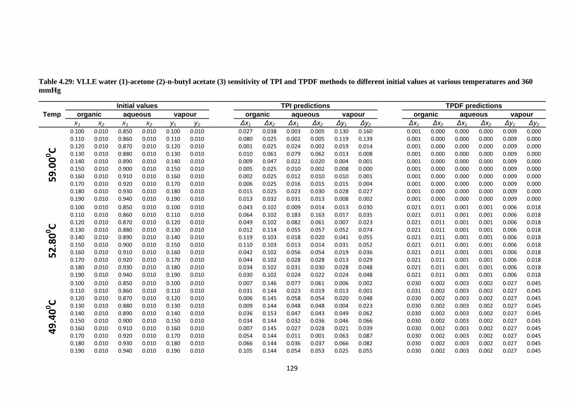
129
Table 4.29: VLLE water (1)-acetone (2)-n-butyl acetate (3) sensitivity of TPI and TPDF methods to different initial values at various temperatures and 360
mmHg
Temp
Initial values TPI predictions TPDF predictions
organic aqueous vapour
organic aqueous vapour
organic aqueous vapour
x1 x2 x1 x2 y1 y2 Δx1 Δx2 Δx1 Δx2 Δy1 Δy2 Δx1 Δx2 Δx1 Δx2 Δy1 Δy2
59
.00
0C
0.100 0.010 0.850 0.010 0.100 0.010
0.027 0.038 0.003 0.005 0.130 0.160
0.001 0.000 0.000 0.000 0.009 0.000
0.110 0.010 0.860 0.010 0.110 0.010
0.080 0.025 0.002 0.005 0.119 0.139
0.001 0.000 0.000 0.000 0.009 0.000
0.120 0.010 0.870 0.010 0.120 0.010
0.001 0.025 0.024 0.002 0.019 0.014
0.001 0.000 0.000 0.000 0.009 0.000
0.130 0.010 0.880 0.010 0.130 0.010
0.010 0.061 0.079 0.062 0.013 0.008
0.001 0.000 0.000 0.000 0.009 0.000
0.140 0.010 0.890 0.010 0.140 0.010
0.009 0.047 0.022 0.020 0.004 0.001
0.001 0.000 0.000 0.000 0.009 0.000
0.150 0.010 0.900 0.010 0.150 0.010
0.005 0.025 0.010 0.002 0.008 0.000
0.001 0.000 0.000 0.000 0.009 0.000
0.160 0.010 0.910 0.010 0.160 0.010
0.002 0.025 0.012 0.010 0.010 0.001
0.001 0.000 0.000 0.000 0.009 0.000
0.170 0.010 0.920 0.010 0.170 0.010
0.006 0.025 0.016 0.015 0.015 0.004
0.001 0.000 0.000 0.000 0.009 0.000
0.180 0.010 0.930 0.010 0.180 0.010
0.015 0.025 0.023 0.030 0.028 0.027
0.001 0.000 0.000 0.000 0.009 0.000
0.190 0.010 0.940 0.010 0.190 0.010
0.013 0.032 0.031 0.013 0.008 0.002
0.001 0.000 0.000 0.000 0.009 0.000
52
.80
0C
0.100 0.010 0.850 0.010 0.100 0.010
0.043 0.102 0.009 0.014 0.013 0.030
0.021 0.011 0.001 0.001 0.006 0.018
0.110 0.010 0.860 0.010 0.110 0.010
0.064 0.102 0.183 0.163 0.017 0.035
0.021 0.011 0.001 0.001 0.006 0.018
0.120 0.010 0.870 0.010 0.120 0.010
0.049 0.102 0.082 0.061 0.007 0.023
0.021 0.011 0.001 0.001 0.006 0.018
0.130 0.010 0.880 0.010 0.130 0.010
0.012 0.114 0.055 0.057 0.052 0.074
0.021 0.011 0.001 0.001 0.006 0.018
0.140 0.010 0.890 0.010 0.140 0.010
0.119 0.103 0.018 0.020 0.041 0.055
0.021 0.011 0.001 0.001 0.006 0.018
0.150 0.010 0.900 0.010 0.150 0.010
0.110 0.103 0.013 0.014 0.031 0.052
0.021 0.011 0.001 0.001 0.006 0.018
0.160 0.010 0.910 0.010 0.160 0.010
0.042 0.102 0.056 0.054 0.019 0.036
0.021 0.011 0.001 0.001 0.006 0.018
0.170 0.010 0.920 0.010 0.170 0.010
0.044 0.102 0.028 0.028 0.013 0.029
0.021 0.011 0.001 0.001 0.006 0.018
0.180 0.010 0.930 0.010 0.180 0.010
0.034 0.102 0.031 0.030 0.028 0.048
0.021 0.011 0.001 0.001 0.006 0.018
0.190 0.010 0.940 0.010 0.190 0.010
0.030 0.102 0.024 0.022 0.024 0.048
0.021 0.011 0.001 0.001 0.006 0.018
49
.40
0C
0.100 0.010 0.850 0.010 0.100 0.010
0.007 0.146 0.077 0.061 0.006 0.002
0.030 0.002 0.003 0.002 0.027 0.045
0.110 0.010 0.860 0.010 0.110 0.010
0.031 0.144 0.023 0.019 0.013 0.001
0.031 0.002 0.003 0.002 0.027 0.045
0.120 0.010 0.870 0.010 0.120 0.010
0.006 0.145 0.058 0.054 0.020 0.048
0.030 0.002 0.003 0.002 0.027 0.045
0.130 0.010 0.880 0.010 0.130 0.010
0.009 0.144 0.048 0.048 0.004 0.023
0.030 0.002 0.003 0.002 0.027 0.045
0.140 0.010 0.890 0.010 0.140 0.010
0.036 0.153 0.047 0.043 0.049 0.062
0.030 0.002 0.003 0.002 0.027 0.045
0.150 0.010 0.900 0.010 0.150 0.010
0.034 0.144 0.032 0.036 0.046 0.066
0.030 0.002 0.003 0.002 0.027 0.045
0.160 0.010 0.910 0.010 0.160 0.010
0.007 0.145 0.027 0.028 0.021 0.039
0.030 0.002 0.003 0.002 0.027 0.045
0.170 0.010 0.920 0.010 0.170 0.010
0.054 0.144 0.011 0.001 0.063 0.087
0.030 0.002 0.003 0.002 0.027 0.045
0.180 0.010 0.930 0.010 0.180 0.010
0.066 0.144 0.036 0.037 0.066 0.082
0.030 0.002 0.003 0.002 0.027 0.045
0.190 0.010 0.940 0.010 0.190 0.010
0.105 0.144 0.054 0.053 0.025 0.055
0.030 0.002 0.003 0.002 0.027 0.045

130
Temp
Initial values TPI predictions TPDF predictions
organic aqueous vapour
organic aqueous vapour
organic aqueous vapour
x1 x2 x1 x2 y1 y2 Δx1 Δx2 Δx1 Δx2 Δy1 Δy2 Δx1 Δx2 Δx1 Δx2 Δy1 Δy2
48
.20
0C
0.100 0.200 0.850 0.010 0.100 0.200
0.078 0.141 0.025 0.029 0.021 0.024
0.005 0.003 0.007 0.007 0.031 0.037 0.110 0.200 0.860 0.010 0.110 0.200
0.111 0.142 0.028 0.027 0.053 0.060
0.005 0.003 0.007 0.007 0.031 0.037
0.120 0.200 0.870 0.010 0.120 0.200
0.196 0.142 0.066 0.063 0.028 0.028
0.005 0.003 0.007 0.007 0.031 0.037 0.130 0.200 0.880 0.010 0.130 0.200
0.077 0.141 0.029 0.029 0.020 0.022
0.005 0.003 0.007 0.007 0.031 0.037
0.140 0.200 0.890 0.010 0.140 0.200
0.117 0.141 0.054 0.054 0.060 0.056
0.005 0.003 0.007 0.007 0.031 0.037 0.150 0.200 0.900 0.010 0.150 0.200
0.091 0.141 0.019 0.025 0.033 0.038
0.005 0.003 0.007 0.007 0.031 0.037
0.160 0.200 0.910 0.010 0.160 0.200
0.114 0.141 0.041 0.041 0.054 0.051
0.005 0.003 0.007 0.007 0.031 0.037 0.170 0.200 0.920 0.010 0.170 0.200
0.075 0.141 0.003 0.007 0.008 0.018
0.005 0.003 0.007 0.007 0.031 0.037
0.180 0.200 0.930 0.010 0.180 0.200
0.110 0.142 0.052 0.049 0.052 0.055
0.005 0.003 0.007 0.007 0.031 0.037 0.190 0.200 0.940 0.010 0.190 0.200
0.053 0.005 0.085 0.078 0.005 0.005
0.005 0.003 0.007 0.007 0.031 0.037
46
.20
0C
0.100 0.200 0.850 0.010 0.100 0.200
0.165 0.330 0.098 0.091 0.144 0.437
0.010 0.027 0.022 0.019 0.024 0.026 0.110 0.200 0.860 0.010 0.110 0.200
0.154 0.136 0.104 0.051 0.003 0.015
0.010 0.027 0.022 0.019 0.024 0.026
0.120 0.200 0.870 0.010 0.120 0.200
0.254 0.392 0.109 0.102 0.410 0.403
0.010 0.027 0.022 0.019 0.024 0.026 0.130 0.200 0.880 0.010 0.130 0.200
0.268 0.131 0.077 0.137 0.056 0.013
0.010 0.027 0.022 0.019 0.024 0.026
0.140 0.200 0.890 0.010 0.140 0.200
0.296 0.131 0.066 0.158 0.061 0.017
0.010 0.027 0.022 0.019 0.024 0.026 0.150 0.200 0.900 0.010 0.150 0.200
0.248 0.131 0.120 0.157 0.069 0.027
0.010 0.027 0.022 0.019 0.024 0.026
0.160 0.200 0.910 0.010 0.160 0.200
0.242 0.131 0.123 0.125 0.065 0.021
0.010 0.027 0.022 0.019 0.024 0.026 0.170 0.200 0.920 0.010 0.170 0.200
0.229 0.131 0.100 0.151 0.084 0.040
0.010 0.027 0.022 0.019 0.024 0.026
0.180 0.200 0.930 0.010 0.180 0.200
0.204 0.249 0.105 0.155 0.090 0.047
0.010 0.027 0.022 0.019 0.024 0.026 0.190 0.200 0.940 0.010 0.190 0.200
0.146 0.133 0.166 0.156 0.086 0.041
0.010 0.027 0.022 0.019 0.024 0.026
45
.10
0C
0.100 0.200 0.850 0.010 0.100 0.200
0.298 0.399 0.123 0.133 0.363 0.419
0.008 0.035 0.067 0.050 0.024 0.025
0.110 0.200 0.860 0.010 0.110 0.200
0.202 0.319 0.101 0.215 0.167 0.408
0.008 0.035 0.067 0.050 0.024 0.025
0.120 0.200 0.870 0.010 0.120 0.200
0.211 0.327 0.136 0.198 0.120 0.408
0.008 0.035 0.067 0.050 0.024 0.025
0.130 0.200 0.880 0.010 0.130 0.200
0.190 0.306 0.114 0.214 0.151 0.408
0.008 0.035 0.067 0.050 0.024 0.025
0.140 0.200 0.890 0.010 0.140 0.200
0.180 0.296 0.188 0.197 0.102 0.408
0.008 0.035 0.067 0.050 0.024 0.025
0.150 0.200 0.900 0.010 0.150 0.200
0.176 0.293 0.190 0.167 0.047 0.410
0.008 0.035 0.067 0.050 0.024 0.025
0.160 0.200 0.910 0.010 0.160 0.200
0.166 0.283 0.195 0.206 0.082 0.408
0.008 0.035 0.067 0.050 0.024 0.025
0.170 0.200 0.920 0.010 0.170 0.200
0.159 0.276 0.201 0.208 0.073 0.408
0.008 0.035 0.067 0.050 0.024 0.025
0.180 0.200 0.930 0.010 0.180 0.200
0.153 0.269 0.177 0.198 0.063 0.408
0.008 0.035 0.067 0.050 0.024 0.025
0.190 0.200 0.940 0.010 0.190 0.200 0.159 0.276 0.173 0.215 0.055 0.451 0.008 0.035 0.067 0.050 0.024 0.025
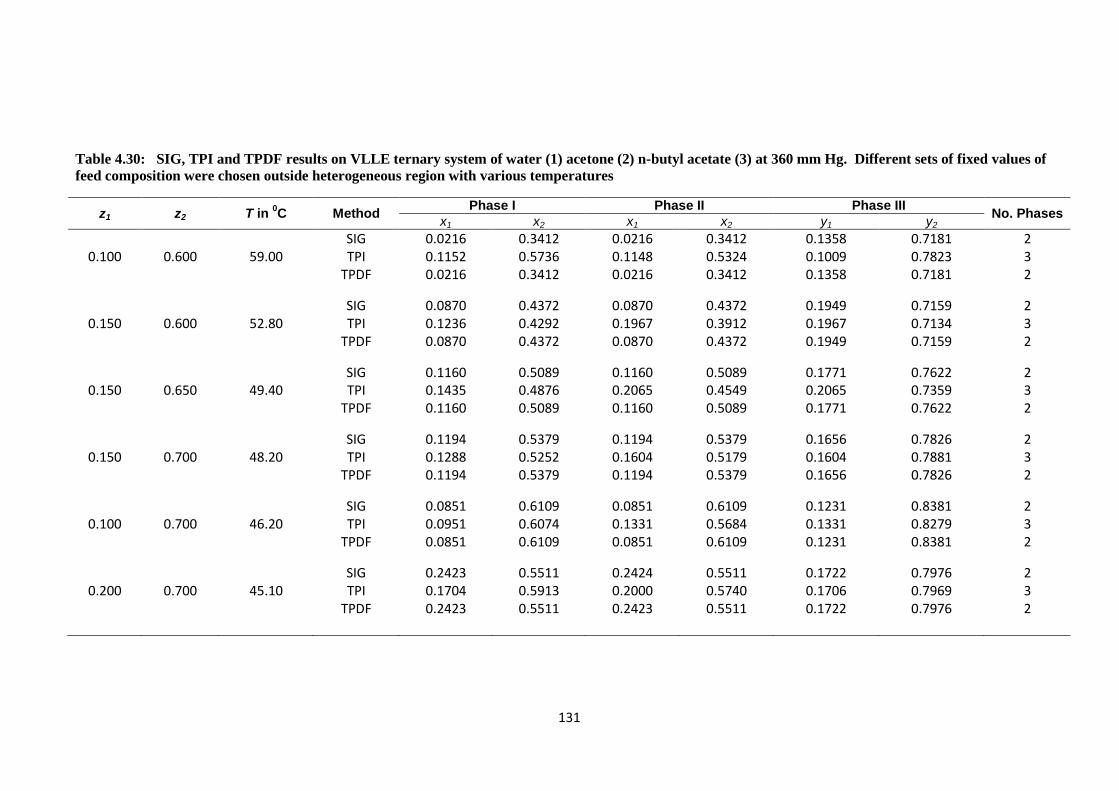
131
Table 4.30: SIG, TPI and TPDF results on VLLE ternary system of water (1) acetone (2) n-butyl acetate (3) at 360 mm Hg. Different sets of fixed values of
feed composition were chosen outside heterogeneous region with various temperatures
z1 z2 T in 0C Method
Phase I Phase II Phase III No. Phases
x1 x2 x1 x2 y1 y2
0.100 0.600 59.00 SIG 0.0216 0.3412 0.0216 0.3412 0.1358 0.7181 2 TPI 0.1152 0.5736 0.1148 0.5324 0.1009 0.7823 3
TPDF 0.0216 0.3412 0.0216 0.3412 0.1358 0.7181 2
0.150 0.600 52.80
SIG 0.0870 0.4372 0.0870 0.4372 0.1949 0.7159 2 TPI 0.1236 0.4292 0.1967 0.3912 0.1967 0.7134 3
TPDF 0.0870 0.4372 0.0870 0.4372 0.1949 0.7159 2
0.150 0.650 49.40
SIG 0.1160 0.5089 0.1160 0.5089 0.1771 0.7622 2 TPI 0.1435 0.4876 0.2065 0.4549 0.2065 0.7359 3
TPDF 0.1160 0.5089 0.1160 0.5089 0.1771 0.7622 2
0.150 0.700 48.20
SIG 0.1194 0.5379 0.1194 0.5379 0.1656 0.7826 2 TPI 0.1288 0.5252 0.1604 0.5179 0.1604 0.7881 3
TPDF 0.1194 0.5379 0.1194 0.5379 0.1656 0.7826 2
0.100 0.700 46.20
SIG 0.0851 0.6109 0.0851 0.6109 0.1231 0.8381 2 TPI 0.0951 0.6074 0.1331 0.5684 0.1331 0.8279 3
TPDF 0.0851 0.6109 0.0851 0.6109 0.1231 0.8381 2
0.200 0.700 45.10
SIG 0.2423 0.5511 0.2424 0.5511 0.1722 0.7976 2 TPI 0.1704 0.5913 0.2000 0.5740 0.1706 0.7969 3
TPDF 0.2423 0.5511 0.2423 0.5511 0.1722 0.7976 2

132
Table 4.31: VLLE ternary system (water-acetone-n-butyl acetate) at 600 mmHg, flash calculation, TPDF and TPI predictions
Temperature Experimental Flash calculation TPDF Prediction TPI Prediction
in 0C
water acetone n-butyl acetate
water acetone n-butyl acetate
water acetone n-butyl acetate
water acetone n-butyl acetate
Organic Phase
69.20 0.188 0.229 0.583
0.176 0.221 0.603
0.192 0.227 0.582
0.190 0.230 0.581
62.40 0.231 0.363 0.406
0.232 0.361 0.408
0.235 0.368 0.397
0.232 0.371 0.398
60.30 0.281 0.420 0.299
0.287 0.412 0.301
0.283 0.419 0.298
0.224 0.440 0.335
58.10 0.352 0.435 0.213
0.352 0.425 0.223
0.343 0.444 0.213
0.362 0.519 0.119 56.50 0.428 0.420 0.151
0.428 0.400 0.172
0.406 0.443 0.151
0.289 0.434 0.277
56.20 0.518 0.376 0.106
0.518 0.367 0.116
0.526 0.378 0.095
0.226 0.495 0.279
Aqueous Phase
69.20 0.968 0.030 0.002
0.972 0.028 0.000
0.969 0.030 0.002
0.970 0.030 0.001
62.40 0.936 0.062 0.003
0.943 0.056 0.001
0.941 0.057 0.002
0.940 0.058 0.002
60.30 0.905 0.091 0.004
0.912 0.085 0.004
0.934 0.065 0.002
0.934 0.062 0.003 58.10 0.872 0.122 0.006
0.886 0.107 0.006
0.892 0.104 0.004
0.864 0.055 0.080
56.50 0.846 0.143 0.010
0.860 0.130 0.009
0.866 0.127 0.006
0.914 0.086 0.000 56.20 0.785 0.198 0.017
0.805 0.175 0.020
0.814 0.173 0.013
0.846 0.143 0.011
Vapour Phase
69.20 0.395 0.463 0.143
0.367 0.465 0.168
0.376 0.481 0.143
0.372 0.486 0.142 62.40 0.313 0.597 0.091
0.287 0.605 0.108
0.271 0.628 0.101
0.268 0.632 0.100
60.30 0.277 0.652 0.070
0.256 0.666 0.078
0.248 0.682 0.070
0.250 0.695 0.055 58.10 0.253 0.692 0.055
0.232 0.709 0.060
0.213 0.733 0.054
0.186 0.703 0.110
56.50 0.244 0.709 0.047
0.223 0.726 0.051
0.192 0.764 0.044
0.289 0.704 0.006
56.20 0.231 0.730 0.040
0.212 0.746 0.042
0.187 0.775 0.038
0.226 0.730 0.044
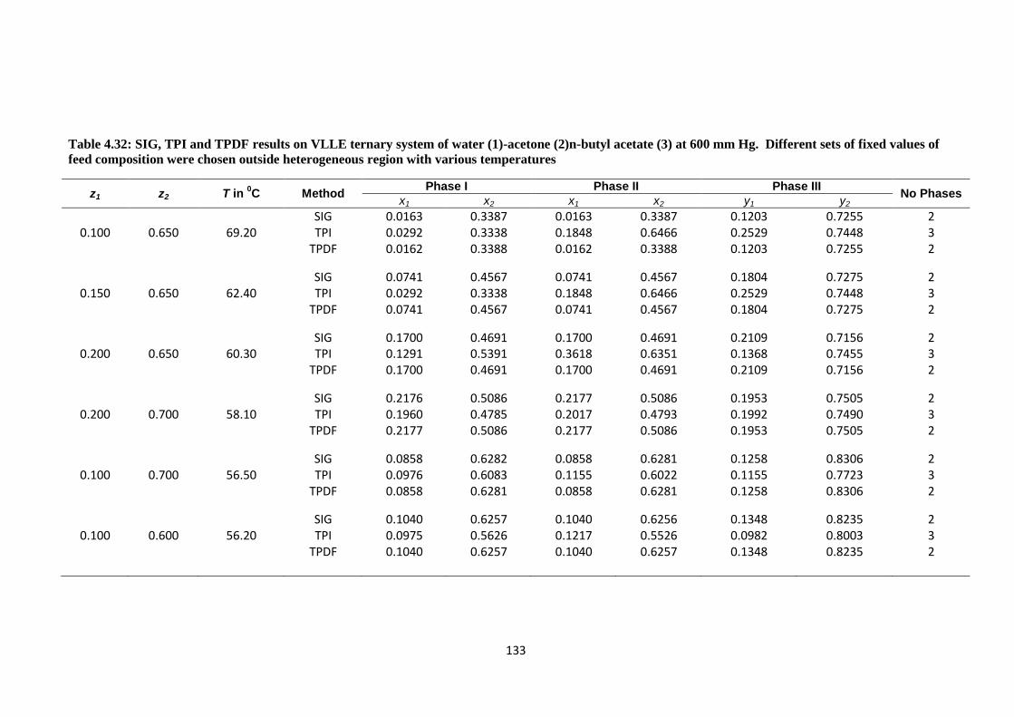
133
Table 4.32: SIG, TPI and TPDF results on VLLE ternary system of water (1)-acetone (2)n-butyl acetate (3) at 600 mm Hg. Different sets of fixed values of
feed composition were chosen outside heterogeneous region with various temperatures
z1 z2 T in 0C Method
Phase I Phase II Phase III No Phases
x1 x2 x1 x2 y1 y2
0.100 0.650 69.20 SIG 0.0163 0.3387 0.0163 0.3387 0.1203 0.7255 2 TPI 0.0292 0.3338 0.1848 0.6466 0.2529 0.7448 3
TPDF 0.0162 0.3388 0.0162 0.3388 0.1203 0.7255 2
0.150 0.650 62.40
SIG 0.0741 0.4567 0.0741 0.4567 0.1804 0.7275 2 TPI 0.0292 0.3338 0.1848 0.6466 0.2529 0.7448 3
TPDF 0.0741 0.4567 0.0741 0.4567 0.1804 0.7275 2
0.200 0.650 60.30
SIG 0.1700 0.4691 0.1700 0.4691 0.2109 0.7156 2 TPI 0.1291 0.5391 0.3618 0.6351 0.1368 0.7455 3
TPDF 0.1700 0.4691 0.1700 0.4691 0.2109 0.7156 2
0.200 0.700 58.10
SIG 0.2176 0.5086 0.2177 0.5086 0.1953 0.7505 2 TPI 0.1960 0.4785 0.2017 0.4793 0.1992 0.7490 3
TPDF 0.2177 0.5086 0.2177 0.5086 0.1953 0.7505 2
0.100 0.700 56.50
SIG 0.0858 0.6282 0.0858 0.6281 0.1258 0.8306 2 TPI 0.0976 0.6083 0.1155 0.6022 0.1155 0.7723 3
TPDF 0.0858 0.6281 0.0858 0.6281 0.1258 0.8306 2
0.100 0.600 56.20
SIG 0.1040 0.6257 0.1040 0.6256 0.1348 0.8235 2 TPI 0.0975 0.5626 0.1217 0.5526 0.0982 0.8003 3
TPDF 0.1040 0.6257 0.1040 0.6257 0.1348 0.8235 2
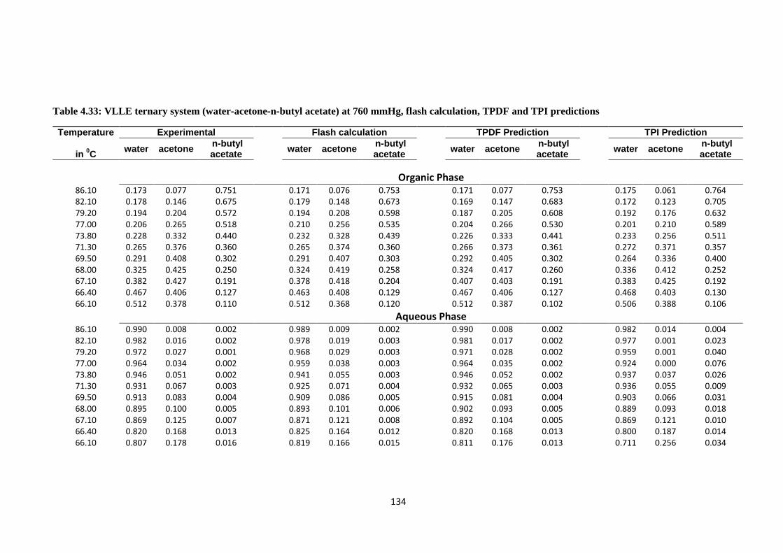
134
Table 4.33: VLLE ternary system (water-acetone-n-butyl acetate) at 760 mmHg, flash calculation, TPDF and TPI predictions
Temperature Experimental Flash calculation TPDF Prediction TPI Prediction
in 0C
water acetone n-butyl acetate
water acetone n-butyl acetate
water acetone n-butyl acetate
water acetone n-butyl acetate
Organic Phase
86.10 0.173 0.077 0.751
0.171 0.076 0.753
0.171 0.077 0.753
0.175 0.061 0.764 82.10 0.178 0.146 0.675
0.179 0.148 0.673
0.169 0.147 0.683
0.172 0.123 0.705
79.20 0.194 0.204 0.572
0.194 0.208 0.598
0.187 0.205 0.608
0.192 0.176 0.632 77.00 0.206 0.265 0.518
0.210 0.256 0.535
0.204 0.266 0.530
0.201 0.210 0.589
73.80 0.228 0.332 0.440
0.232 0.328 0.439
0.226 0.333 0.441
0.233 0.256 0.511 71.30 0.265 0.376 0.360
0.265 0.374 0.360
0.266 0.373 0.361
0.272 0.371 0.357
69.50 0.291 0.408 0.302
0.291 0.407 0.303
0.292 0.405 0.302
0.264 0.336 0.400 68.00 0.325 0.425 0.250
0.324 0.419 0.258
0.324 0.417 0.260
0.336 0.412 0.252
67.10 0.382 0.427 0.191
0.378 0.418 0.204
0.407 0.403 0.191
0.383 0.425 0.192 66.40 0.467 0.406 0.127
0.463 0.408 0.129
0.467 0.406 0.127
0.468 0.403 0.130
66.10 0.512 0.378 0.110
0.512 0.368 0.120
0.512 0.387 0.102
0.506 0.388 0.106
Aqueous Phase
86.10 0.990 0.008 0.002
0.989 0.009 0.002
0.990 0.008 0.002
0.982 0.014 0.004 82.10 0.982 0.016 0.002
0.978 0.019 0.003
0.981 0.017 0.002
0.977 0.001 0.023
79.20 0.972 0.027 0.001
0.968 0.029 0.003
0.971 0.028 0.002
0.959 0.001 0.040 77.00 0.964 0.034 0.002
0.959 0.038 0.003
0.964 0.035 0.002
0.924 0.000 0.076
73.80 0.946 0.051 0.002
0.941 0.055 0.003
0.946 0.052 0.002
0.937 0.037 0.026 71.30 0.931 0.067 0.003
0.925 0.071 0.004
0.932 0.065 0.003
0.936 0.055 0.009
69.50 0.913 0.083 0.004
0.909 0.086 0.005
0.915 0.081 0.004
0.903 0.066 0.031 68.00 0.895 0.100 0.005
0.893 0.101 0.006
0.902 0.093 0.005
0.889 0.093 0.018
67.10 0.869 0.125 0.007
0.871 0.121 0.008
0.892 0.104 0.005
0.869 0.121 0.010 66.40 0.820 0.168 0.013
0.825 0.164 0.012
0.820 0.168 0.013
0.800 0.187 0.014
66.10 0.807 0.178 0.016
0.819 0.166 0.015
0.811 0.176 0.013
0.711 0.256 0.034

135
Temperature Experimental Flash calculation TPDF Prediction TPI Prediction
in 0C
water acetone n-butyl acetate
water acetone n-butyl acetate
water acetone n-butyl acetate
water acetone n-butyl acetate
Vapour Phase
86.10 0.586 0.188 0.226
0.586 0.183 0.232
0.586 0.188 0.226
0.550 0.126 0.324 82.10 0.484 0.336 0.179
0.497 0.320 0.183
0.485 0.335 0.179
0.496 0.333 0.171
79.20 0.424 0.423 0.153
0.437 0.412 0.151
0.427 0.423 0.150
0.414 0.425 0.161 77.00 0.394 0.474 0.133
0.397 0.475 0.128
0.394 0.474 0.131
0.425 0.502 0.072
73.80 0.338 0.562 0.100
0.342 0.561 0.097
0.341 0.564 0.095
0.350 0.579 0.071 71.30 0.304 0.614 0.081
0.309 0.611 0.079
0.309 0.610 0.081
0.273 0.570 0.157
69.50 0.282 0.650 0.068
0.287 0.647 0.066
0.283 0.648 0.069
0.264 0.617 0.119 68.00 0.276 0.665 0.059
0.274 0.667 0.059
0.267 0.664 0.069
0.236 0.642 0.122
67.10 0.267 0.682 0.051
0.262 0.685 0.052
0.262 0.679 0.059
0.197 0.636 0.166 66.40 0.247 0.712 0.041
0.246 0.713 0.041
0.247 0.712 0.041
0.184 0.651 0.165
66.10 0.262 0.693 0.046
0.256 0.698 0.046
0.237 0.718 0.045
0.182 0.655 0.163

136
Table 4.34: Results for the SIG, TPI and TPDF methods on VLLE ternary system of water (1)-acetone (2)n-butyl acetate (3) at 760 mm Hg. Different sets of
fixed values of feed composition were chosen outside heterogeneous region with various temperatures
z1 z2 T in 0C Method
Phase I Phase II Phase III No Phases
x1 x2 x1 x2 y1 y2
0.200 0.500 86.10 SIG 0.0513 0.2153 0.0513 0.2153 0.2319 0.5611 2 TPI 0.0513 0.2153 0.2611 0.4681 0.2752 0.7007 3
TPDF 0.0514 0.2152 0.0514 0.2152 0.2319 0.5611 2
0.200 0.600 82.10
SIG 0.0572 0.2686 0.0572 0.2686 0.2110 0.6256 2 TPI 0.0981 0.1785 0.4384 0.5605 0.0894 0.8637 3
TPDF 0.0572 0.2686 0.0572 0.2686 0.2110 0.6255 2
0.200 0.700 79.20
SIG 0.0894 0.3817 0.0894 0.3817 0.2103 0.7360 2 TPI 0.1731 0.2043 0.2030 0.6961 0.0763 0.8279 3
TPDF 0.0894 0.3816 0.0894 0.3816 0.2003 0.7008 2
0.200 0.500 77.00
SIG 0.1043 0.3163 0.1043 0.3163 0.2622 0.6193 2 TPI 0.1974 0.2424 0.2053 0.2404 0.0885 0.7721 3
TPDF 0.1044 0.3162 0.1044 0.3162 0.2622 0.6193 2
0.200 0.600 73.80
SIG 0.1129 0.3787 0.1129 0.3787 0.2305 0.6775 2 TPI 0.1045 0.3766 0.2881 0.5728 0.0120 0.6950 3
TPDF 0.1128 0.3787 0.1128 0.3787 0.2305 0.6775 2
0.250 0.650 71.30
SIG 0.1692 0.4074 0.1692 0.4074 0.2566 0.6699 2 TPI 0.0978 0.4388 0.2933 0.5874 0.0193 0.6962 3
TPDF 0.1692 0.4074 0.1692 0.4074 0.2566 0.6699 2
0.100 0.650 69.50
SIG 0.0746 0.5025 0.0746 0.5025 0.1277 0.8108 2 TPI 0.0810 0.4891 0.2677 0.6222 0.0267 0.6976 3
TPDF 0.0746 0.5025 0.0746 0.5025 0.1277 0.8108 2

137
z1 z2 T in 0C Method
Phase I Phase II Phase III No Phases
x1 x2 x1 x2 y1 y2
0.150 0.750 68.00 SIG 0.1113 0.5181 0.1113 0.5181 0.1568 0.7908 2 TPI 0.0601 0.3867 0.1704 0.7428 0.0473 0.7717 3
TPDF 0.1113 0.5181 0.1113 0.5181 0.1568 0.7908 2
0.100 0.750 67.10 SIG 0.0768 0.5592 0.0768 0.5592 0.1111 0.8414 2 TPI 0.0649 0.4341 0.1327 0.7309 0.0093 0.7644 3
TPDF 0.0768 0.5592 0.0768 0.5592 0.1111 0.8414 2
0.150 0.800 66.40
SIG 0.1232 0.5528 0.1232 0.5528 0.1507 0.8061 2 TPI 0.1133 0.5080 0.1514 0.7185 0.1133 0.7342 3
TPDF 0.1232 0.5528 0.1232 0.5528 0.1507 0.8061 2
0.100 0.650 66.10
SIG 0.1997 0.5279 0.1997 0.5279 0.1974 0.7626 2 TPI 0.1996 0.4033 0.2411 0.3886 0.0884 0.7909 3
TPDF 0.1997 0.5279 0.1997 0.5279 0.1974 0.7626 2
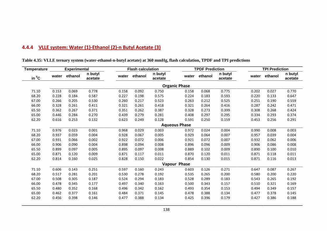
138
4.4.4 VLLE system: Water (1)-Ethanol (2)-n Butyl Acetate (3)
Table 4.35: VLLE ternary system (water-ethanol-n-butyl acetate) at 360 mmHg, flash calculation, TPDF and TPI predictions
Temperature Experimental Flash calculation TPDF Prediction TPI Prediction
in 0C
water ethanol n butyl acetate
water ethanol n butyl acetate
water ethanol n butyl acetate
water ethanol n butyl acetate
Organic Phase
71.10 0.153 0.069 0.778
0.158 0.092 0.750
0.158 0.068 0.775
0.202 0.027 0.770 68.20 0.228 0.184 0.587
0.227 0.198 0.575
0.224 0.183 0.593
0.220 0.133 0.647
67.00 0.266 0.205 0.530
0.260 0.217 0.523
0.263 0.212 0.525
0.251 0.190 0.559 66.00 0.328 0.261 0.411
0.321 0.261 0.418
0.321 0.264 0.416
0.287 0.242 0.471
65.50 0.362 0.267 0.371
0.351 0.262 0.387
0.328 0.273 0.399
0.308 0.268 0.424 65.00 0.446 0.284 0.270
0.439 0.279 0.281
0.408 0.297 0.295
0.334 0.293 0.374
62.20 0.616 0.253 0.132
0.623 0.249 0.128
0.591 0.250 0.159
0.453 0.256 0.291
Aqueous Phase
71.10 0.976 0.023 0.001
0.968 0.029 0.003
0.972 0.024 0.004
0.990 0.008 0.003 68.20 0.937 0.059 0.004
0.928 0.067 0.005
0.929 0.064 0.007
0.957 0.039 0.004
67.00 0.931 0.066 0.002
0.922 0.072 0.006
0.921 0.072 0.007
0.932 0.062 0.006 66.00 0.906 0.090 0.004
0.898 0.094 0.008
0.896 0.096 0.009
0.906 0.086 0.008
65.50 0.899 0.097 0.005
0.895 0.097 0.008
0.889 0.102 0.009
0.890 0.100 0.010 65.00 0.871 0.120 0.009
0.871 0.117 0.011
0.870 0.120 0.011
0.871 0.118 0.011
62.20 0.814 0.160 0.025
0.828 0.150 0.022
0.854 0.130 0.015
0.871 0.116 0.013
Vapour Phase
71.10 0.606 0.143 0.251
0.597 0.160 0.243
0.603 0.126 0.271
0.647 0.087 0.267 68.20 0.517 0.281 0.201
0.530 0.278 0.192
0.535 0.265 0.200
0.580 0.200 0.220
67.00 0.508 0.305 0.187
0.524 0.294 0.183
0.528 0.289 0.183
0.543 0.265 0.192 66.00 0.478 0.345 0.177
0.497 0.340 0.163
0.500 0.343 0.157
0.510 0.321 0.169
65.50 0.480 0.352 0.168
0.496 0.342 0.162
0.493 0.354 0.153
0.494 0.349 0.157 65.00 0.462 0.377 0.161
0.484 0.371 0.145
0.478 0.388 0.134
0.477 0.378 0.145
62.20 0.456 0.398 0.146
0.477 0.388 0.134
0.425 0.396 0.179
0.427 0.386 0.188

139
Table 4.36: SIG, TPI and TPDF results on VLLE ternary system of water (1)-ethanol (2) n-butyl acetate (3) at 360 mm Hg. Different sets of fixed values of
feed composition were chosen outside heterogeneous region with various temperatures
z1 z2 T in 0C Method
Phase I Phase II Phase III No Phases
x1 x2 x1 x2 y1 y2
0.100 0.600 71.10 SIG 0.0184 0.4408 0.0183 0.4408 0.1384 0.6736 2 TPI 0.0001 0.3027 0.1001 0.3983 0.0859 0.6620 3
TPDF 0.0165 0.4427 0.0165 0.4427 0.1379 0.6737 2
0.150 0.600 68.20
SIG 0.0328 0.4789 0.0328 0.4789 0.1985 0.6499 2 TPI 0.0364 0.6445 0.1560 0.4612 0.1552 0.8165 3
TPDF 0.0330 0.4787 0.0330 0.4787 0.1983 0.6499 2
0.150 0.650 67.00
SIG 0.0310 0.5324 0.0310 0.5324 0.1866 0.6851 2 TPI 0.1489 0.4211 0.3094 0.3800 0.1848 0.7597 3
TPDF 0.0314 0.5319 0.0314 0.5319 0.1857 0.6852 2
0.150 0.700 66.00
SIG 0.0282 0.5834 0.0283 0.5833 0.1737 0.7190 2 TPI 0.0094 0.6404 0.1607 0.4577 0.1607 0.6920 3
TPDF 0.0264 0.5852 0.0264 0.5852 0.1707 0.7196 2
0.100 0.700 65.50
SIG 0.0227 0.6233 0.0227 0.6232 0.1518 0.7510 2 TPI 0.0363 0.7312 0.1002 0.5746 0.1002 0.8003 3
TPDF 0.0217 0.6243 0.0217 0.6243 0.1515 0.7510 2
0.200 0.700 65.00
SIG 0.0377 0.5927 0.0378 0.5926 0.2023 0.7048 2 TPI 0.0653 0.6396 0.2000 0.4860 0.1993 0.7518 3
TPDF 0.0376 0.5928 0.0376 0.5928 0.2004 0.7003 2
0.150 0.700 62.20 SIG 0.0493 0.6701 0.0508 0.6689 0.2171 0.7188 2 TPI 0.0275 0.8054 0.1502 0.6085 0.1502 0.7750 3
TPDF 0.0488 0.6706 0.0488 0.6706 0.2152 0.7191 2
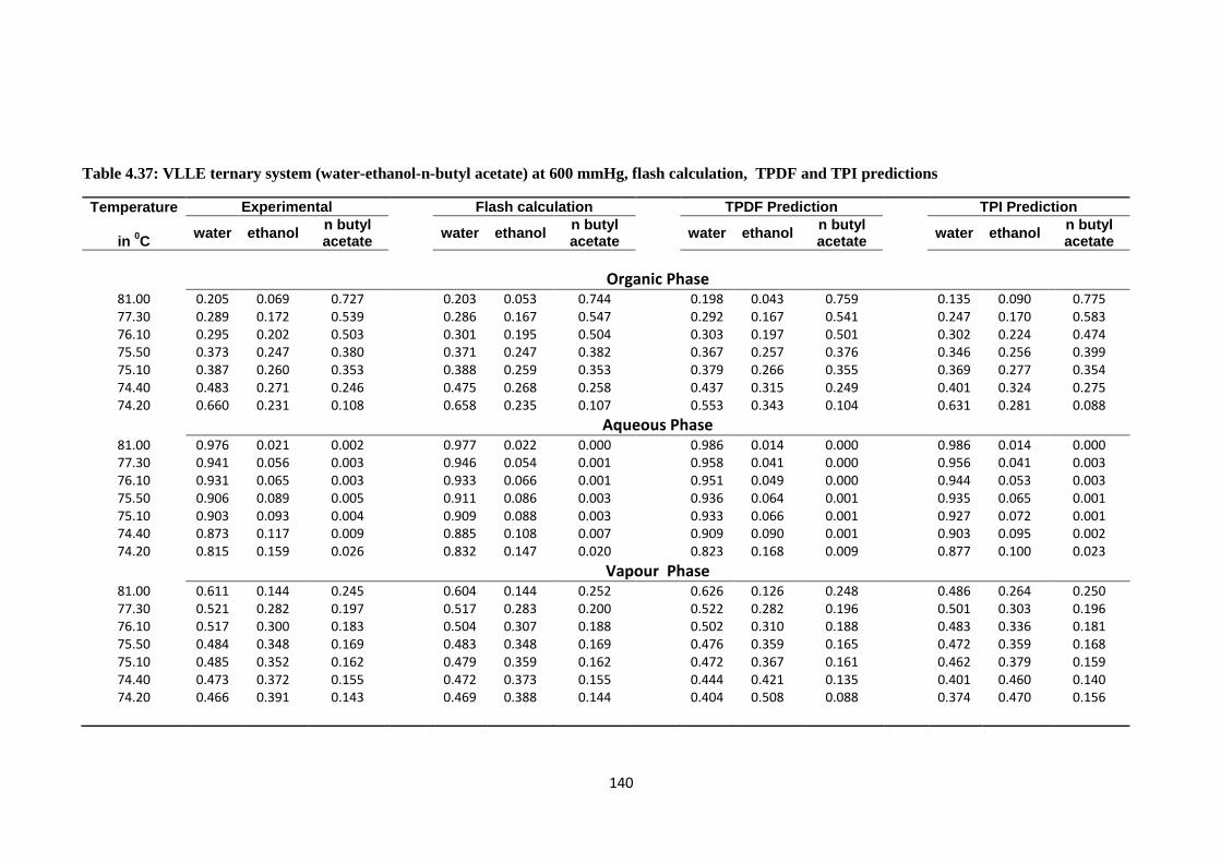
140
Table 4.37: VLLE ternary system (water-ethanol-n-butyl acetate) at 600 mmHg, flash calculation, TPDF and TPI predictions
Temperature Experimental Flash calculation TPDF Prediction TPI Prediction
in 0C
water ethanol n butyl acetate
water ethanol n butyl acetate
water ethanol n butyl acetate
water ethanol n butyl acetate
Organic Phase
81.00 0.205 0.069 0.727
0.203 0.053 0.744
0.198 0.043 0.759
0.135 0.090 0.775 77.30 0.289 0.172 0.539
0.286 0.167 0.547
0.292 0.167 0.541
0.247 0.170 0.583
76.10 0.295 0.202 0.503
0.301 0.195 0.504
0.303 0.197 0.501
0.302 0.224 0.474 75.50 0.373 0.247 0.380
0.371 0.247 0.382
0.367 0.257 0.376
0.346 0.256 0.399
75.10 0.387 0.260 0.353
0.388 0.259 0.353
0.379 0.266 0.355
0.369 0.277 0.354 74.40 0.483 0.271 0.246
0.475 0.268 0.258
0.437 0.315 0.249
0.401 0.324 0.275
74.20 0.660 0.231 0.108
0.658 0.235 0.107
0.553 0.343 0.104
0.631 0.281 0.088
Aqueous Phase
81.00 0.976 0.021 0.002
0.977 0.022 0.000
0.986 0.014 0.000
0.986 0.014 0.000 77.30 0.941 0.056 0.003
0.946 0.054 0.001
0.958 0.041 0.000
0.956 0.041 0.003
76.10 0.931 0.065 0.003
0.933 0.066 0.001
0.951 0.049 0.000
0.944 0.053 0.003 75.50 0.906 0.089 0.005
0.911 0.086 0.003
0.936 0.064 0.001
0.935 0.065 0.001
75.10 0.903 0.093 0.004
0.909 0.088 0.003
0.933 0.066 0.001
0.927 0.072 0.001 74.40 0.873 0.117 0.009
0.885 0.108 0.007
0.909 0.090 0.001
0.903 0.095 0.002
74.20 0.815 0.159 0.026
0.832 0.147 0.020
0.823 0.168 0.009
0.877 0.100 0.023
Vapour Phase
81.00 0.611 0.144 0.245
0.604 0.144 0.252
0.626 0.126 0.248
0.486 0.264 0.250 77.30 0.521 0.282 0.197
0.517 0.283 0.200
0.522 0.282 0.196
0.501 0.303 0.196
76.10 0.517 0.300 0.183
0.504 0.307 0.188
0.502 0.310 0.188
0.483 0.336 0.181 75.50 0.484 0.348 0.169
0.483 0.348 0.169
0.476 0.359 0.165
0.472 0.359 0.168
75.10 0.485 0.352 0.162
0.479 0.359 0.162
0.472 0.367 0.161
0.462 0.379 0.159 74.40 0.473 0.372 0.155
0.472 0.373 0.155
0.444 0.421 0.135
0.401 0.460 0.140
74.20 0.466 0.391 0.143
0.469 0.388 0.144
0.404 0.508 0.088
0.374 0.470 0.156

141
Table 4.38: SIG, TPI and TPDF results on VLLE ternary system of water (1)-ethanol (2) n-butyl acetate (3) at 600 mm Hg. Different sets of fixed values of
feed composition were chosen outside heterogeneous region with various temperatures
z1 z2 T in 0C Method
Phase I Phase II Phase III No Phases
x1 x2 x1 x2 y1 y2
0.100 0.600 81.00 SIG 0.0241 0.3926 0.0241 0.3926 0.1247 0.6678 2 TPI 0.0389 0.3311 0.1872 0.5946 0.1872 0.8020 3
TPDF 0.0194 0.3973 0.0194 0.3973 0.1248 0.6678 2
0.150 0.600 77.30
SIG 0.0528 0.4783 0.0528 0.4783 0.1906 0.6508 2 TPI 0.0702 0.4267 0.2323 0.5986 0.2447 0.7497 3
TPDF 0.0529 0.4782 0.0529 0.4782 0.1906 0.6508 2
0.150 0.650 76.10
SIG 0.0464 0.5131 0.0464 0.5131 0.1711 0.6779 2 TPI 0.0586 0.4741 0.2006 0.6390 0.2063 0.7477 3
TPDF 0.0464 0.5132 0.0464 0.5132 0.1711 0.6779 2
0.150 0.700 75.50
SIG 0.0497 0.6027 0.0497 0.6027 0.1650 0.7145 2 TPI 0.0524 0.6032 0.1612 0.6955 0.2620 0.7190 3
TPDF 0.0493 0.6031 0.0493 0.6031 0.1650 0.7145 2
0.100 0.700 75.10
SIG 0.0437 0.6482 0.0437 0.6482 0.1478 0.7440 2 TPI 0.0601 0.5938 0.1852 0.6976 0.2003 0.7320 3
TPDF 0.0437 0.6482 0.0437 0.6482 0.1478 0.7440 2
0.200 0.700 74.40
SIG 0.0769 0.6337 0.0769 0.6337 0.2042 0.7138 2 TPI 0.0922 0.5595 0.3034 0.6955 0.1075 0.7766 3
TPDF 0.0769 0.6337 0.0769 0.6337 0.2003 0.7002 2
0.200 0.600 74.20 SIG 0.1116 0.5449 0.1116 0.5449 0.2512 0.6319 2 TPI 0.1458 0.4921 0.2000 0.4534 0.1862 0.7716 3
TPDF 0.1116 0.5449 0.1116 0.5449 0.2512 0.6319 2

142
Table 4.39: VLLE ternary system (water-ethanol-n-butyl acetate) at 760 mmHg, flash calculation, TPDF and TPI predictions
Temperature Experimental Flash calculation TPDF Prediction TPI Prediction
in 0C water ethanol
n-butyl acetate
water ethanol n-butyl acetate
water ethanol n-butyl acetate
water ethanol n-butyl acetate
Organic Phase
88.20 0.188 0.058 0.754
0.191 0.068 0.741
0.189 0.068 0.743
0.213 0.060 0.727 86.10 0.226 0.118 0.656
0.229 0.125 0.645
0.224 0.126 0.650
0.228 0.109 0.663
85.00 0.290 0.188 0.522
0.294 0.185 0.521
0.279 0.184 0.537
0.250 0.188 0.562 84.50 0.303 0.206 0.491
0.310 0.206 0.485
0.311 0.206 0.483
0.274 0.209 0.517
84.10 0.385 0.253 0.362
0.386 0.248 0.365
0.384 0.248 0.368
0.291 0.225 0.485 83.50 0.408 0.256 0.336
0.406 0.252 0.342
0.410 0.254 0.337
0.292 0.262 0.446
83.20 0.500 0.265 0.235
0.497 0.266 0.237
0.490 0.281 0.230
0.370 0.273 0.357 83.10 0.533 0.265 0.202
0.531 0.266 0.203
0.504 0.277 0.218
0.422 0.278 0.300
82.80 0.650 0.233 0.117
0.647 0.242 0.111
0.608 0.292 0.100
0.482 0.301 0.217
Aqueous Phase
88.20 0.978 0.020 0.002
0.976 0.017 0.007
0.974 0.019 0.007
0.975 0.018 0.007 86.10 0.956 0.042 0.002
0.954 0.037 0.009
0.954 0.039 0.007
0.947 0.031 0.022
85.00 0.942 0.055 0.002
0.933 0.057 0.010
0.929 0.062 0.009
0.933 0.059 0.008 84.50 0.935 0.062 0.002
0.923 0.067 0.010
0.919 0.072 0.009
0.932 0.064 0.003
84.10 0.911 0.084 0.005
0.898 0.090 0.012
0.897 0.093 0.010
0.924 0.104 0.028 83.50 0.898 0.093 0.009
0.888 0.098 0.014
0.896 0.094 0.010
0.917 0.076 0.007
83.20 0.876 0.115 0.009
0.870 0.114 0.015
0.876 0.113 0.011
0.842 0.132 0.026 83.10 0.867 0.122 0.011
0.862 0.121 0.017
0.880 0.109 0.011
0.899 0.096 0.005
82.80 0.825 0.149 0.025
0.825 0.149 0.026
0.830 0.153 0.017
0.876 0.102 0.022
Vapour Phase
88.20 0.619 0.139 0.243
0.628 0.111 0.260
0.618 0.120 0.262
0.627 0.113 0.260 86.10 0.556 0.217 0.227
0.580 0.194 0.226
0.569 0.205 0.227
0.433 0.362 0.206
85.00 0.532 0.274 0.194
0.541 0.268 0.192
0.530 0.276 0.194
0.407 0.355 0.238 84.50 0.521 0.300 0.178
0.528 0.292 0.180
0.520 0.298 0.182
0.415 0.367 0.218
84.10 0.493 0.340 0.167
0.500 0.340 0.159
0.501 0.339 0.160
0.407 0.379 0.214 83.50 0.496 0.344 0.160
0.498 0.345 0.158
0.501 0.342 0.157
0.460 0.372 0.168
83.20 0.481 0.368 0.151
0.488 0.367 0.145
0.488 0.367 0.145
0.345 0.472 0.183 83.10 0.481 0.374 0.145
0.485 0.372 0.143
0.491 0.364 0.145
0.321 0.520 0.159
82.80 0.471 0.387 0.141 0.476 0.383 0.141 0.471 0.394 0.135 0.473 0.387 0.140
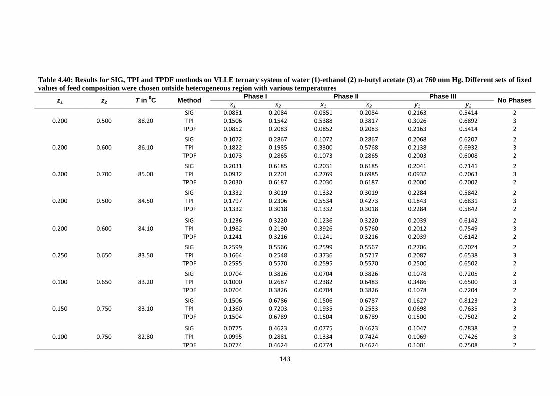
143
Table 4.40: Results for SIG, TPI and TPDF methods on VLLE ternary system of water (1)-ethanol (2) n-butyl acetate (3) at 760 mm Hg. Different sets of fixed
values of feed composition were chosen outside heterogeneous region with various temperatures
z1 z2 T in 0C Method
Phase I Phase II Phase III No Phases
x1 x2 x1 x2 y1 y2
0.200 0.500 88.20 SIG 0.0851 0.2084 0.0851 0.2084 0.2163 0.5414 2 TPI 0.1506 0.1542 0.5388 0.3817 0.3026 0.6892 3
TPDF 0.0852 0.2083 0.0852 0.2083 0.2163 0.5414 2
0.200 0.600 86.10
SIG 0.1072 0.2867 0.1072 0.2867 0.2068 0.6207 2 TPI 0.1822 0.1985 0.3300 0.5768 0.2138 0.6932 3
TPDF 0.1073 0.2865 0.1073 0.2865 0.2003 0.6008 2
0.200 0.700 85.00
SIG 0.2031 0.6185 0.2031 0.6185 0.2041 0.7141 2 TPI 0.0932 0.2201 0.2769 0.6985 0.0932 0.7063 3
TPDF 0.2030 0.6187 0.2030 0.6187 0.2000 0.7002 2
0.200 0.500 84.50
SIG 0.1332 0.3019 0.1332 0.3019 0.2284 0.5842 2 TPI 0.1797 0.2306 0.5534 0.4273 0.1843 0.6831 3
TPDF 0.1332 0.3018 0.1332 0.3018 0.2284 0.5842 2
0.200 0.600 84.10
SIG 0.1236 0.3220 0.1236 0.3220 0.2039 0.6142 2 TPI 0.1982 0.2190 0.3926 0.5760 0.2012 0.7549 3
TPDF 0.1241 0.3216 0.1241 0.3216 0.2039 0.6142 2
0.250 0.650 83.50
SIG 0.2599 0.5566 0.2599 0.5567 0.2706 0.7024 2 TPI 0.1664 0.2548 0.3736 0.5717 0.2087 0.6538 3
TPDF 0.2595 0.5570 0.2595 0.5570 0.2500 0.6502 2
0.100 0.650 83.20
SIG 0.0704 0.3826 0.0704 0.3826 0.1078 0.7205 2 TPI 0.1000 0.2687 0.2382 0.6483 0.3486 0.6500 3
TPDF 0.0704 0.3826 0.0704 0.3826 0.1078 0.7204 2
0.150 0.750 83.10
SIG 0.1506 0.6786 0.1506 0.6787 0.1627 0.8123 2 TPI 0.1360 0.7203 0.1935 0.2553 0.0698 0.7635 3
TPDF 0.1504 0.6789 0.1504 0.6789 0.1500 0.7502 2
0.100 0.750 82.80
SIG 0.0775 0.4623 0.0775 0.4623 0.1047 0.7838 2
TPI 0.0995 0.2881 0.1334 0.7424 0.1069 0.7426 3
TPDF 0.0774 0.4624 0.0774 0.4624 0.1001 0.7508 2
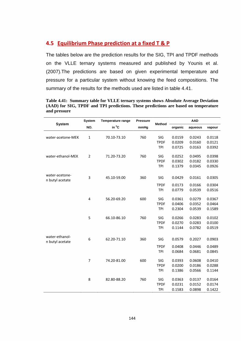
144
4.5 Equilibrium Phase prediction at a fixed T & P
The tables below are the prediction results for the SIG, TPI and TPDF methods
on the VLLE ternary systems measured and published by Younis et al.
(2007).The predictions are based on given experimental temperature and
pressure for a particular system without knowing the feed compositions. The
summary of the results for the methods used are listed in table 4.41.
Table 4.41: Summary table for VLLE ternary systems shows Absolute Average Deviation
(AAD) for SIG, TPDF and TPI predictions. These predictions are based on temperature
and pressure
System System Temperature range Pressure
Method AAD
NO. in 0C mmHg organic aqueous vapour
water-acetone-MEK 1 70.10-73.10 760 SIG 0.0159 0.0243 0.0118
TPDF 0.0209 0.0160 0.0121
TPI 0.0725 0.0163 0.0392
water-ethanol-MEK 2 71.20-73.20 760 SIG 0.0252 0.0495 0.0398
TPDF 0.0302 0.0182 0.0330
TPI 0.1379 0.0345 0.0926
water-acetone- n butyl acetate
3 45.10-59.00 360 SIG 0.0429 0.0161 0.0305
TPDF 0.0173 0.0166 0.0304
TPI 0.0779 0.0539 0.0516
4 56.20-69.20 600 SIG 0.0361 0.0279 0.0367
TPDF 0.0406 0.0352 0.0464
TPI 0.2304 0.0539 0.1589
5 66.10-86.10 760 SIG 0.0266 0.0283 0.0102
TPDF 0.0270 0.0283 0.0100
TPI 0.1144 0.0782 0.0519
water-ethanol- n butyl acetate
6 62.20-71.10 360 SIG 0.0579 0.2027 0.0903
TPDF 0.0408 0.0446 0.0489
TPI 0.0684 0.0681 0.0845
7 74.20-81.00 600 SIG 0.0393 0.0608 0.0410
TPDF 0.0200 0.0186 0.0288
TPI 0.1386 0.0566 0.1144
8 82.80-88.20 760 SIG 0.0363 0.0137 0.0164
TPDF 0.0231 0.0152 0.0174
TPI 0.1583 0.0898 0.1422
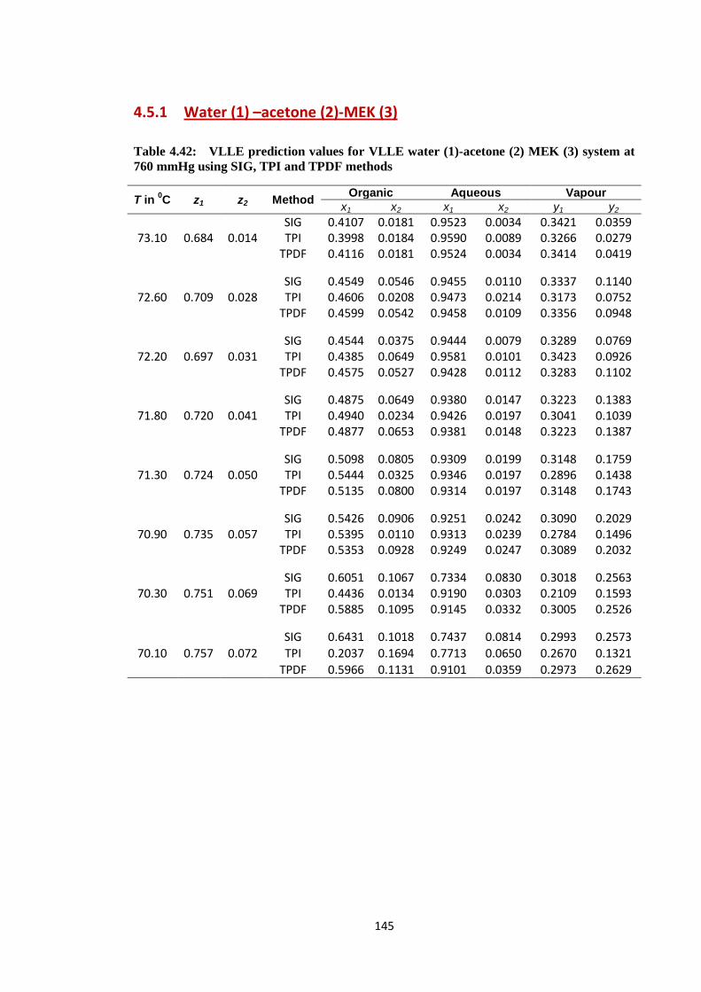
145
4.5.1 Water (1) –acetone (2)-MEK (3)
Table 4.42: VLLE prediction values for VLLE water (1)-acetone (2) MEK (3) system at
760 mmHg using SIG, TPI and TPDF methods
T in 0C z1 z2 Method
Organic Aqueous Vapour
x1 x2 x1 x2 y1 y2
73.10 0.684 0.014 SIG 0.4107 0.0181 0.9523 0.0034 0.3421 0.0359 TPI 0.3998 0.0184 0.9590 0.0089 0.3266 0.0279
TPDF 0.4116 0.0181 0.9524 0.0034 0.3414 0.0419
72.60 0.709 0.028
SIG 0.4549 0.0546 0.9455 0.0110 0.3337 0.1140 TPI 0.4606 0.0208 0.9473 0.0214 0.3173 0.0752
TPDF 0.4599 0.0542 0.9458 0.0109 0.3356 0.0948
72.20 0.697 0.031
SIG 0.4544 0.0375 0.9444 0.0079 0.3289 0.0769 TPI 0.4385 0.0649 0.9581 0.0101 0.3423 0.0926
TPDF 0.4575 0.0527 0.9428 0.0112 0.3283 0.1102
71.80 0.720 0.041
SIG 0.4875 0.0649 0.9380 0.0147 0.3223 0.1383 TPI 0.4940 0.0234 0.9426 0.0197 0.3041 0.1039
TPDF 0.4877 0.0653 0.9381 0.0148 0.3223 0.1387
71.30 0.724 0.050
SIG 0.5098 0.0805 0.9309 0.0199 0.3148 0.1759 TPI 0.5444 0.0325 0.9346 0.0197 0.2896 0.1438
TPDF 0.5135 0.0800 0.9314 0.0197 0.3148 0.1743
70.90 0.735 0.057
SIG 0.5426 0.0906 0.9251 0.0242 0.3090 0.2029 TPI 0.5395 0.0110 0.9313 0.0239 0.2784 0.1496
TPDF 0.5353 0.0928 0.9249 0.0247 0.3089 0.2032
70.30 0.751 0.069
SIG 0.6051 0.1067 0.7334 0.0830 0.3018 0.2563 TPI 0.4436 0.0134 0.9190 0.0303 0.2109 0.1593
TPDF 0.5885 0.1095 0.9145 0.0332 0.3005 0.2526
70.10 0.757 0.072
SIG 0.6431 0.1018 0.7437 0.0814 0.2993 0.2573
TPI 0.2037 0.1694 0.7713 0.0650 0.2670 0.1321
TPDF 0.5966 0.1131 0.9101 0.0359 0.2973 0.2629

146
4.5.2 Water (1) –ethanol (2)-MEK (3)
Table 4.43: VLLE prediction values for VLLE water (1)-ethanol (2) MEK (3) system at
760 mmHg using SIG, TPI and TPDF methods
T in 0C z1 z2 Method
Organic Aqueous Vapour
x1 x2 x1 x2 y1 y2
73.20 0.705 0.009
SIG 0.4594 0.0441 0.9432 0.0151 0.3389 0.0694
TPI 0.1376 0.0901 0.8970 0.0016 0.5242 0.0429
TPDF 0.4313 0.0463 0.9419 0.0166 0.3473 0.0198
72.80 0.726 0.021
SIG 0.5276 0.0460 0.9359 0.0159 0.3329 0.0661
TPI 0.1584 0.0818 0.9005 0.0014 0.5164 0.0411
TPDF 0.4954 0.0550 0.9344 0.0192 0.3382 0.0452
72.10 0.713 0.041
SIG 0.5190 0.0539 0.9137 0.0221 0.3222 0.0741
TPI 0.4915 0.0547 0.9537 0.0029 0.4441 0.0626
TPDF 0.5189 0.0575 0.9149 0.0231 0.3219 0.0791
71.60 0.695 0.055
SIG 0.5585 0.0686 0.5587 0.0686 0.3208 0.0922
TPI 0.5704 0.0142 0.8608 0.0643 0.3627 0.0944
TPDF 0.5692 0.0710 0.9024 0.0298 0.3206 0.0955
71.20 0.780 0.061
SIG 0.7441 0.0645 0.7778 0.0590 0.3086 0.1023
TPI 0.3819 0.1001 0.7629 0.0748 0.7826 0.0667
TPDF 0.6994 0.0690 0.7416 0.0633 0.3033 0.1045
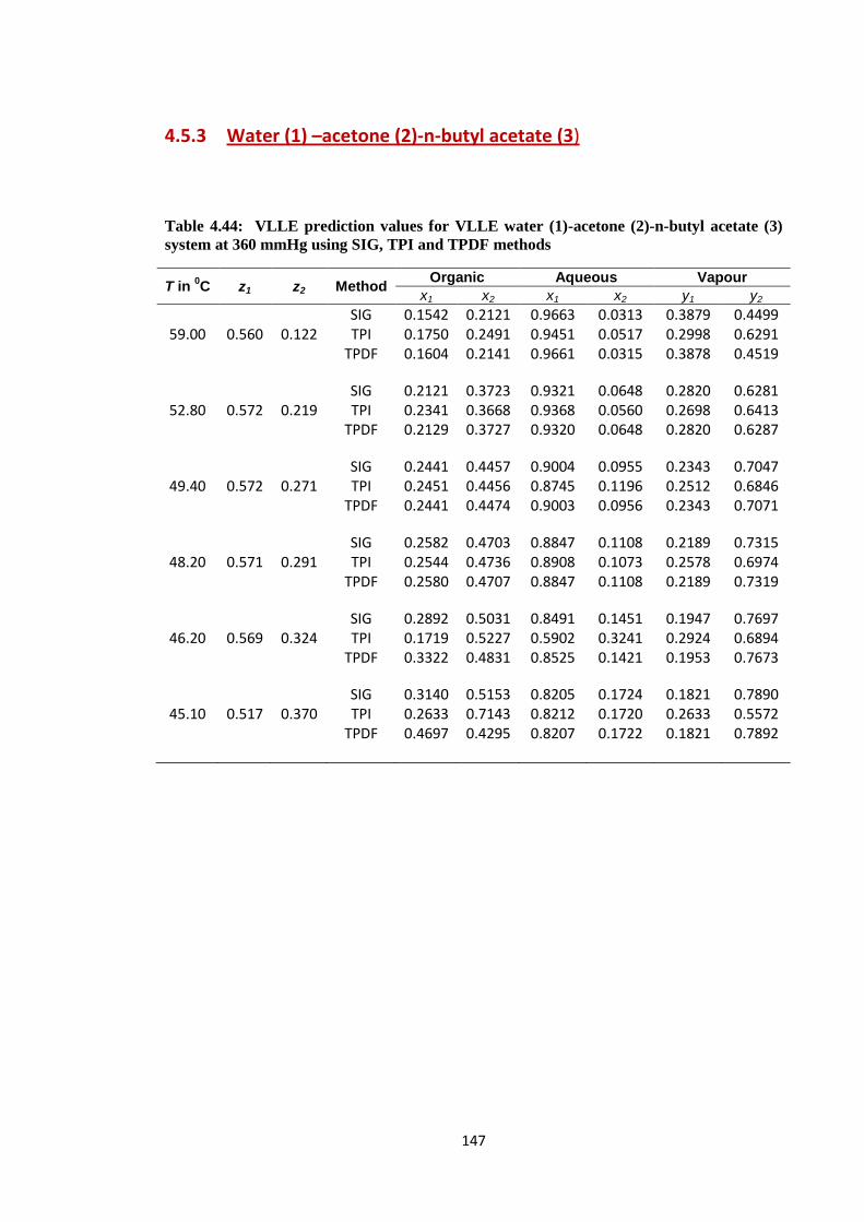
147
4.5.3 Water (1) –acetone (2)-n-butyl acetate (3)
Table 4.44: VLLE prediction values for VLLE water (1)-acetone (2)-n-butyl acetate (3)
system at 360 mmHg using SIG, TPI and TPDF methods
T in 0C z1 z2 Method
Organic Aqueous Vapour
x1 x2 x1 x2 y1 y2
59.00 0.560 0.122 SIG 0.1542 0.2121 0.9663 0.0313 0.3879 0.4499 TPI 0.1750 0.2491 0.9451 0.0517 0.2998 0.6291
TPDF 0.1604 0.2141 0.9661 0.0315 0.3878 0.4519
52.80 0.572 0.219 SIG 0.2121 0.3723 0.9321 0.0648 0.2820 0.6281 TPI 0.2341 0.3668 0.9368 0.0560 0.2698 0.6413
TPDF 0.2129 0.3727 0.9320 0.0648 0.2820 0.6287
49.40 0.572 0.271 SIG 0.2441 0.4457 0.9004 0.0955 0.2343 0.7047 TPI 0.2451 0.4456 0.8745 0.1196 0.2512 0.6846
TPDF 0.2441 0.4474 0.9003 0.0956 0.2343 0.7071
48.20 0.571 0.291 SIG 0.2582 0.4703 0.8847 0.1108 0.2189 0.7315 TPI 0.2544 0.4736 0.8908 0.1073 0.2578 0.6974
TPDF 0.2580 0.4707 0.8847 0.1108 0.2189 0.7319
46.20 0.569 0.324 SIG 0.2892 0.5031 0.8491 0.1451 0.1947 0.7697 TPI 0.1719 0.5227 0.5902 0.3241 0.2924 0.6894
TPDF 0.3322 0.4831 0.8525 0.1421 0.1953 0.7673
45.10 0.517 0.370
SIG 0.3140 0.5153 0.8205 0.1724 0.1821 0.7890 TPI 0.2633 0.7143 0.8212 0.1720 0.2633 0.5572
TPDF 0.4697 0.4295 0.8207 0.1722 0.1821 0.7892
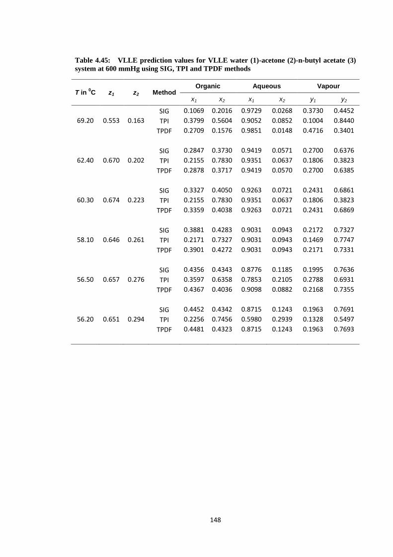
148
Table 4.45: VLLE prediction values for VLLE water (1)-acetone (2)-n-butyl acetate (3)
system at 600 mmHg using SIG, TPI and TPDF methods
T in 0C z1 z2 Method
Organic Aqueous Vapour
x1 x2 x1 x2 y1 y2
69.20 0.553 0.163
SIG 0.1069 0.2016 0.9729 0.0268 0.3730 0.4452
TPI 0.3799 0.5604 0.9052 0.0852 0.1004 0.8440
TPDF 0.2709 0.1576 0.9851 0.0148 0.4716 0.3401
62.40 0.670 0.202
SIG 0.2847 0.3730 0.9419 0.0571 0.2700 0.6376
TPI 0.2155 0.7830 0.9351 0.0637 0.1806 0.3823
TPDF 0.2878 0.3717 0.9419 0.0570 0.2700 0.6385
60.30 0.674 0.223
SIG 0.3327 0.4050 0.9263 0.0721 0.2431 0.6861
TPI 0.2155 0.7830 0.9351 0.0637 0.1806 0.3823
TPDF 0.3359 0.4038 0.9263 0.0721 0.2431 0.6869
58.10 0.646 0.261
SIG 0.3881 0.4283 0.9031 0.0943 0.2172 0.7327
TPI 0.2171 0.7327 0.9031 0.0943 0.1469 0.7747
TPDF 0.3901 0.4272 0.9031 0.0943 0.2171 0.7331
56.50 0.657 0.276
SIG 0.4356 0.4343 0.8776 0.1185 0.1995 0.7636
TPI 0.3597 0.6358 0.7853 0.2105 0.2788 0.6931
TPDF 0.4367 0.4036 0.9098 0.0882 0.2168 0.7355
56.20 0.651 0.294
SIG 0.4452 0.4342 0.8715 0.1243 0.1963 0.7691
TPI 0.2256 0.7456 0.5980 0.2939 0.1328 0.5497
TPDF 0.4481 0.4323 0.8715 0.1243 0.1963 0.7693

149
Table 4.46: VLLE prediction values for VLLE water (1)-acetone (2)-n-butyl acetate (3)
system at 760 mmHg using SIG, TPI and TPDF methods
T in 0C z1 z2 Method
Organic Aqueous Vapour
x1 x2 x1 x2 y1 y2
86.10 0.584 0.045
SIG 0.1819 0.0843 0.9908 0.0079 0.5906 0.1941
TPI 0.1075 0.1129 0.6543 0.3211 0.6899 0.2031
TPDF 0.1734 0.0766 0.9915 0.0072 0.5909 0.1827
82.10 0.585 0.084
SIG 0.1862 0.1510 0.9834 0.0152 0.5020 0.3193
TPI 0.1410 0.1694 0.7984 0.0399 0.4746 0.4273
TPDF 0.1915 0.1529 0.9833 0.0154 0.5019 0.3224
79.20 0.586 0.115
SIG 0.1966 0.2080 0.9764 0.0222 0.4444 0.4114
TPI 0.1966 0.2079 0.7916 0.0416 0.4444 0.4114
TPDF 0.2013 0.2093 0.9763 0.0224 0.4444 0.4122
77.00 0.589 0.141
SIG 0.2072 0.2524 0.9702 0.0284 0.4044 0.4736
TPI 0.1608 0.2115 0.9380 0.0395 0.4122 0.5571
TPDF 0.2097 0.2533 0.9701 0.0285 0.4044 0.4743
73.80 0.594 0.180
SIG 0.2289 0.3198 0.9591 0.0394 0.3514 0.5553
TPI 0.1952 0.2299 0.9473 0.0451 0.4114 0.5841
TPDF 0.2305 0.3209 0.9590 0.0395 0.3514 0.5562
71.30 0.601 0.212
SIG 0.2559 0.3740 0.9476 0.0507 0.3139 0.6133
TPI 0.2076 0.2727 0.9548 0.0362 0.3870 0.5940
TPDF 0.2556 0.3748 0.9476 0.0507 0.3139 0.6139
69.50 0.609 0.237
SIG 0.2824 0.4116 0.9369 0.0613 0.2889 0.6518
TPI 0.2105 0.2969 0.9518 0.0411 0.4139 0.5789
TPDF 0.2816 0.4124 0.9368 0.0613 0.2889 0.6524
68.00 0.618 0.256
SIG 0.3119 0.4398 0.9252 0.0728 0.2692 0.6825
TPI 0.1608 0.6740 0.8810 0.1135 0.2960 0.4281
TPDF 0.3109 0.4405 0.9252 0.0728 0.2691 0.6828
67.10 0.626 0.267
SIG 0.3345 0.4535 0.9163 0.0815 0.2578 0.7001
TPI 0.1147 0.7993 0.9267 0.0687 0.2848 0.6692
TPDF 0.3334 0.4542 0.9164 0.0815 0.2578 0.7003
66.40 0.632 0.276
SIG 0.3562 0.4615 0.9079 0.0898 0.2492 0.7137
TPI 0.2397 0.6988 0.9069 0.0904 0.2397 0.6988
TPDF 0.3548 0.4622 0.9080 0.0897 0.2492 0.7136
66.10 0.635 0.279
SIG 0.3669 0.4636 0.9037 0.0938 0.2455 0.7190
TPI 0.6350 0.3099 0.6898 0.2513 0.2210 0.6550
TPDF 0.3654 0.4645 0.9038 0.0937 0.2455 0.7193
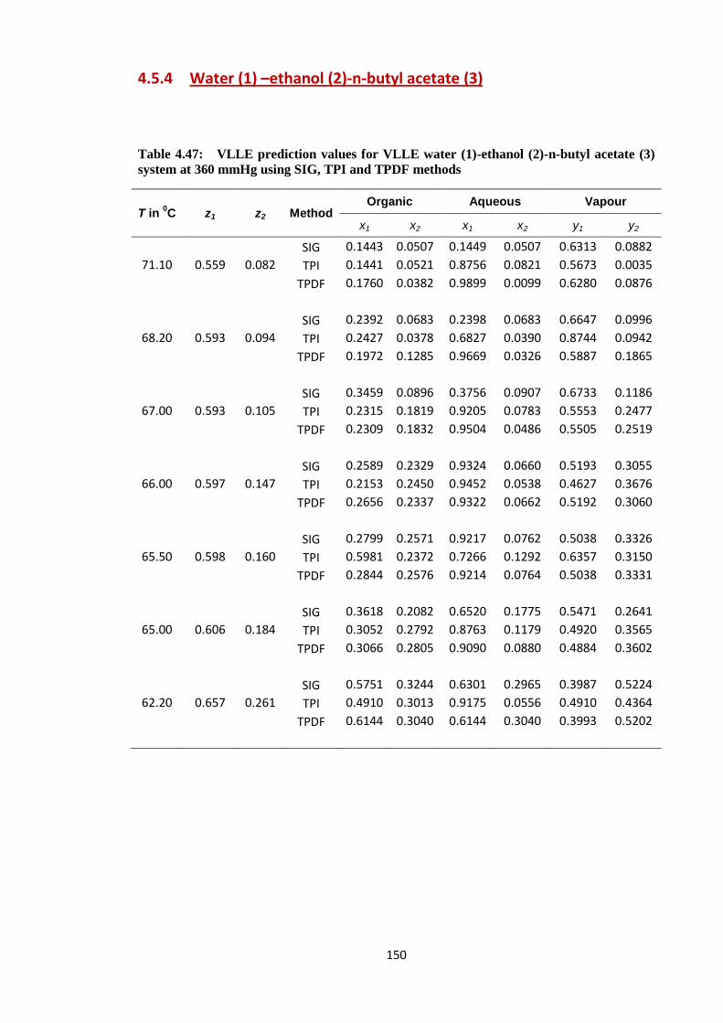
150
4.5.4 Water (1) –ethanol (2)-n-butyl acetate (3)
Table 4.47: VLLE prediction values for VLLE water (1)-ethanol (2)-n-butyl acetate (3)
system at 360 mmHg using SIG, TPI and TPDF methods
T in 0C z1 z2 Method
Organic Aqueous Vapour
x1 x2 x1 x2 y1 y2
71.10 0.559 0.082
SIG 0.1443 0.0507 0.1449 0.0507 0.6313 0.0882
TPI 0.1441 0.0521 0.8756 0.0821 0.5673 0.0035
TPDF 0.1760 0.0382 0.9899 0.0099 0.6280 0.0876
68.20 0.593 0.094
SIG 0.2392 0.0683 0.2398 0.0683 0.6647 0.0996
TPI 0.2427 0.0378 0.6827 0.0390 0.8744 0.0942
TPDF 0.1972 0.1285 0.9669 0.0326 0.5887 0.1865
67.00 0.593 0.105
SIG 0.3459 0.0896 0.3756 0.0907 0.6733 0.1186
TPI 0.2315 0.1819 0.9205 0.0783 0.5553 0.2477
TPDF 0.2309 0.1832 0.9504 0.0486 0.5505 0.2519
66.00 0.597 0.147
SIG 0.2589 0.2329 0.9324 0.0660 0.5193 0.3055
TPI 0.2153 0.2450 0.9452 0.0538 0.4627 0.3676
TPDF 0.2656 0.2337 0.9322 0.0662 0.5192 0.3060
65.50 0.598 0.160
SIG 0.2799 0.2571 0.9217 0.0762 0.5038 0.3326
TPI 0.5981 0.2372 0.7266 0.1292 0.6357 0.3150
TPDF 0.2844 0.2576 0.9214 0.0764 0.5038 0.3331
65.00 0.606 0.184
SIG 0.3618 0.2082 0.6520 0.1775 0.5471 0.2641
TPI 0.3052 0.2792 0.8763 0.1179 0.4920 0.3565
TPDF 0.3066 0.2805 0.9090 0.0880 0.4884 0.3602
62.20 0.657 0.261
SIG 0.5751 0.3244 0.6301 0.2965 0.3987 0.5224
TPI 0.4910 0.3013 0.9175 0.0556 0.4910 0.4364
TPDF 0.6144 0.3040 0.6144 0.3040 0.3993 0.5202

151
Table 4.48: VLLE prediction values for VLLE water (1)-ethanol (2)-n-butyl acetate (3)
system at 600 mmHg using SIG, TPI and TPDF methods
T in 0C z1 z2 Method
Organic Aqueous Vapour
x1 x2 x1 x2 y1 y2
81.00 0.591 0.045
SIG 0.2432 0.0215 0.2443 0.0215 0.6915 0.0527
TPI 0.2207 0.0513 0.7623 0.0880 0.6061 0.1212
TPDF 0.2220 0.0349 0.9887 0.0106 0.6099 0.1326
77.30 0.615 0.114
SIG 0.2813 0.1747 0.9457 0.0525 0.5126 0.2914
TPI 0.2737 0.1746 0.8855 0.0623 0.5102 0.2941
TPDF 0.2875 0.1765 0.9454 0.0528 0.5125 0.2926
76.10 0.613 0.134
SIG 0.3361 0.2318 0.9256 0.0716 0.4810 0.3460
TPI 0.4724 0.3971 0.9493 0.0141 0.4713 0.5277
TPDF 0.3371 0.2325 0.9254 0.0717 0.4810 0.3465
75.50 0.639 0.168
SIG 0.3727 0.2615 0.9121 0.0842 0.4652 0.3746
TPI 0.4573 0.4834 0.8652 0.1259 0.3077 0.6882
TPDF 0.3696 0.2620 0.9120 0.0843 0.4652 0.3749
75.10 0.645 0.176
SIG 0.3999 0.2803 0.9010 0.0944 0.4547 0.3943
TPI 0.4467 0.5070 0.8152 0.1826 0.4258 0.5671
TPDF 0.3952 0.2811 0.9009 0.0945 0.4546 0.3947
74.40 0.678 0.194
SIG 0.4552 0.3083 0.8747 0.1183 0.4357 0.4314
TPI 0.5514 0.4474 0.8379 0.1530 0.3753 0.6211
TPDF 0.4506 0.3095 0.8747 0.1183 0.4357 0.4316
74.20 0.738 0.195
SIG 0.4732 0.3144 0.8646 0.1273 0.4302 0.4427
TPI 0.3852 0.6000 0.8537 0.1442 0.5654 0.4335
TPDF 0.6889 0.2339 0.6889 0.2339 0.4354 0.4353
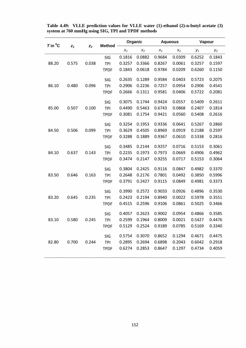
152
Table 4.49: VLLE prediction values for VLLE water (1)-ethanol (2)-n-butyl acetate (3)
system at 760 mmHg using SIG, TPI and TPDF methods
T in 0C z1 z2 Method
Organic Aqueous Vapour
x1 x2 x1 x2 y1 y2
88.20 0.575 0.038
SIG 0.1816 0.0882 0.9684 0.0309 0.6252 0.1843
TPI 0.3257 0.3366 0.8267 0.0061 0.3257 0.1597
TPDF 0.1843 0.0618 0.9784 0.0209 0.6260 0.1150
86.10 0.480 0.096
SIG 0.2635 0.1289 0.9584 0.0403 0.5723 0.2075
TPI 0.2906 0.2236 0.7257 0.0954 0.2906 0.4541
TPDF 0.2666 0.1311 0.9581 0.0406 0.5722 0.2081
85.00 0.507 0.100
SIG 0.3075 0.1744 0.9424 0.0557 0.5409 0.2611
TPI 0.4490 0.5463 0.6743 0.0868 0.2407 0.1814
TPDF 0.3081 0.1754 0.9421 0.0560 0.5408 0.2616
84.50
SIG 0.3254 0.1953 0.9336 0.0641 0.5267 0.2860
0.506 0.099 TPI 0.3629 0.4505 0.8969 0.0919 0.2188 0.2597
TPDF 0.3288 0.1889 0.9367 0.0610 0.5338 0.2816
84.10 0.637 0.143
SIG 0.3485 0.2144 0.9257 0.0716 0.5153 0.3061
TPI 0.2235 0.1973 0.7973 0.0669 0.4906 0.4962
TPDF 0.3474 0.2147 0.9255 0.0717 0.5153 0.3064
83.50 0.646 0.163
SIG 0.3804 0.2425 0.9116 0.0847 0.4982 0.3370
TPI 0.2648 0.2176 0.7801 0.0492 0.3850 0.5996
TPDF 0.3791 0.2427 0.9115 0.0849 0.4981 0.3373
83.20 0.645 0.235
SIG 0.3990 0.2572 0.9033 0.0926 0.4896 0.3530
TPI 0.2423 0.2194 0.8940 0.0022 0.5978 0.3551
TPDF 0.4515 0.2596 0.9106 0.0861 0.5025 0.3466
83.10 0.580 0.245
SIG 0.4057 0.2623 0.9002 0.0954 0.4866 0.3585
TPI 0.2599 0.1964 0.8009 0.0021 0.5427 0.4476
TPDF 0.5129 0.2524 0.9189 0.0785 0.5169 0.3340
82.80 0.700 0.244
SIG 0.5754 0.3070 0.8652 0.1294 0.4671 0.4475
TPI 0.2895 0.2694 0.6898 0.2043 0.6042 0.2918
TPDF 0.6274 0.2853 0.8647 0.1297 0.4734 0.4059
153
4.6 Discussion on VLLE ternary systems
The main intention of this section of research has been to apply the TPI
developed by Hodges et al. (1998) to recently available new VLLE ternary
experimental data. Further tests examine the reliability and efficiency of this
method in predicting the phase equilibrium for heterogeneous multicomponent
systems.
In the application of the TPI method to VLLE binary systems, (𝜏) was defined
as the part of the Tangent line bounded by the Gibbs energy curve (𝜙) and to
minimise the Gibbs free energy, the (𝜏) function has to be minimised.
There are two independent variables in binary systems (𝛼1, 𝛼2) when a 2-point
search method is used. This number increases to three if the direct 3-point
search method is used. However applying the TPI to ternary systems is more
complicated than binary systems, as the tangent changes to a 2D area of
intersection with the (𝜙) surface in a 3D composition space; in this environment
the (𝜏) function has to be minimised.
The number of variables required in a ternary 3-phase search increases to six
(𝛼1, 𝛼2, 𝛼3, 𝜃1, 𝜃2 and 𝜃3) , where 𝛼𝑖 represents the length of an arm extending
from the feed composition (𝑧𝑖) at an angle (𝜃𝑖) . The Nelder-Mead algorithm is
constrained to search for optimum values for both variables (𝛼𝑖 is constrained to
stay in the physical composition space and 𝜃𝑖values in a range of (0-360)). The
tangent plane now represents the area of a 2D composition plane and the
slopes of this tangent plane (𝑚1𝑇𝑃 , 𝑚2𝑇𝑃) are determined by solving the
objective function (𝜏 = 𝜏 + ∆𝜏). The Nelder-Mead technique requires a set of
initial values to set up the simplex. The minimisation algorithm evaluates the
value of the (𝜏) function for a number of iterations and generates new variables
based on four coefficient factors (reflection, expansion, contraction and
shrinkage). This process reduces the function value to zero by rejecting the
largest value and replacing the variables with new evaluated values. The initial
composition and the feed composition are used to calculate the starting values
for these variables(𝛼𝑖, 𝜃𝑖). If the (𝜏) value is reduced to zero, this indicates
solutions have been found and the global Gibbs free energy is at the minimum

154
level. The Nelder-Mead minimisation procedure is explained in a previous
chapter (3.12) and its algorithm can be found in appendix C.
The ∆𝜏 for ternary systems now takes the form of the following equation;
∆𝜏 = ℎ1√(1 + (𝑚1𝑇𝑃)2 ℎ2√(1 + (𝑚2𝑇𝑃)2 (4.9)
where ℎ1 and ℎ2 are the width of a unit of the search grid , 𝑚1𝑇𝑃 and 𝑚2𝑇𝑃
are the slopes of the tangent plane.
4.6.1 Application of the TPI and TPDF methods on artificial ternary systems
Shyu et al. (1995) designed two hypothetical ternary systems using the
Margules excess Gibbs energy model which is based on three binary constants.
Initially the TPI method was applied to these two ternary 3-phase systems
(artificial test systems; 1 and 2 of Shyu et.al (1995)), at a grid size (100x100)
using fixed initial compositions and various (𝑧1 , 𝑧2) overall feed compositions.
TPI requires the division of the composition space into a number of grids. A
number of sets of the grid were tested in a range of (50-500). It was found that
using the small grid number produces 𝜏 > 0 and the large number greatly
increases the computational time without further improvement in the results.
This work has selected the optimum grid number (100 x100). When the
selected grid failed in producing 𝜏 = 0 solution, the number was increased to a
higher value. Figure 4.18 shows various grid numbers versus overall AAD for
composition for both systems of Shyu et al. (1995).
Figure 4.18: A plot of the grid number against the Absolute Average Deviation for
composition for the artificial systems of Shyu et al. (1995)
0.0000
0.0005
0.0010
0.0015
0.0020
0.0025
0.0030
50 100 150 200 250 300 350 400 450 500 550
System 1
System 2
Grid No.
𝐴𝐴
𝐷 𝑥
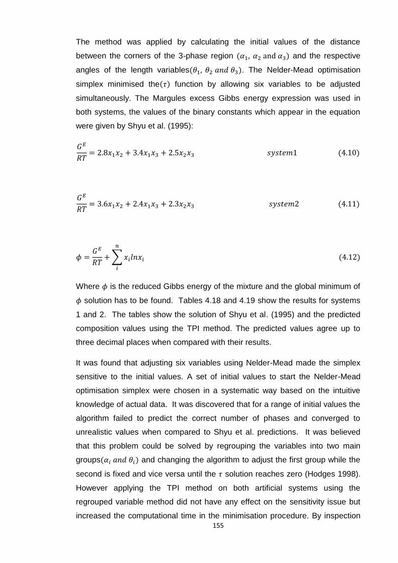
155
The method was applied by calculating the initial values of the distance
between the corners of the 3-phase region (𝛼1, 𝛼2 and 𝛼3) and the respective
angles of the length variables(𝜃1, 𝜃2 𝑎𝑛𝑑 𝜃3). The Nelder-Mead optimisation
simplex minimised the(𝜏) function by allowing six variables to be adjusted
simultaneously. The Margules excess Gibbs energy expression was used in
both systems, the values of the binary constants which appear in the equation
were given by Shyu et al. (1995):
𝐺𝐸
𝑅𝑇= 2.8𝑥1𝑥2 + 3.4𝑥1𝑥3 + 2.5𝑥2𝑥3 𝑠𝑦𝑠𝑡𝑒𝑚1 (4.10)
𝐺𝐸
𝑅𝑇= 3.6𝑥1𝑥2 + 2.4𝑥1𝑥3 + 2.3𝑥2𝑥3 𝑠𝑦𝑠𝑡𝑒𝑚2 (4.11)
𝜙 =𝐺𝐸
𝑅𝑇+ ∑ 𝑥𝑖𝑙𝑛𝑥𝑖
𝑛
𝑖
(4.12)
Where 𝜙 is the reduced Gibbs energy of the mixture and the global minimum of
𝜙 solution has to be found. Tables 4.18 and 4.19 show the results for systems
1 and 2. The tables show the solution of Shyu et al. (1995) and the predicted
composition values using the TPI method. The predicted values agree up to
three decimal places when compared with their results.
It was found that adjusting six variables using Nelder-Mead made the simplex
sensitive to the initial values. A set of initial values to start the Nelder-Mead
optimisation simplex were chosen in a systematic way based on the intuitive
knowledge of actual data. It was discovered that for a range of initial values the
algorithm failed to predict the correct number of phases and converged to
unrealistic values when compared to Shyu et al. predictions. It was believed
that this problem could be solved by regrouping the variables into two main
groups(𝛼𝑖 𝑎𝑛𝑑 𝜃𝑖) and changing the algorithm to adjust the first group while the
second is fixed and vice versa until the 𝜏 solution reaches zero (Hodges 1998).
However applying the TPI method on both artificial systems using the
regrouped variable method did not have any effect on the sensitivity issue but
increased the computational time in the minimisation procedure. By inspection

156
of these initial values shown in tables (4.18 & 4.19), a set of values was
selected to start the Nelder-Mead simplex and conclusions were drawn about
the behaviour of the TPI method. The necessity of a systematic approach to the
selection of Nelder-Mead initial values emphasised by this work and a
systematic approach is proposed for real systems later in this chapter.
Two different sets of feed compositions were selected for both systems; the
values of the first set were inside the 3-phase region and the second sets of
values were outside the 3-phase region. The TPI test results for the first region
showed that the prediction values are in the 3-phase heterogeneous region. It
was noticed that the TPI method procedure could converge to solutions that
gave two identical phase compositions when the feed compositions were
outside the 3-phase region. In this case the objective function produced shows
𝜏 > 0.
When the feed compositions are outside the 3-phase region, the results indicate
that the TPI predictions are consistent with a 2-phase region. However,
according to the phase diagram published by Shyu et al. (1995) for these
systems, some of these feed compositions are in the single phase region which
TPI fails to identify. These results show that the TPI method is capable of
differentiating between 3-phase and 2-phase regions. But there are problems
over the whole phase range.
In order to apply the TPDF method on both hypothetical systems, the excess
Gibbs energy equation should be changed to an activity coefficient form
because the TPDF Gibbs free minimisation function suggested by
Michelsen(1982 a) takes the following form:
𝐹(𝑦)
𝑅𝑇= ∑ 𝑦𝑖(𝑙𝑛𝑦𝑖 + 𝑙𝑛𝛾𝑖(𝑦) − 𝑙𝑛𝑧𝑖 − 𝑙𝑛𝛾𝑖(𝑧)) (4.13)
𝑖
The simplified Margules equation for excess Gibbs energy for a ternary system
is based on consideration of the three components being chemically similar and
the assumption that they have similar molecular size. The equation has three
binary constants (A12, A13 & A23):
gE
𝑅𝑇= 𝐴12 𝑥1𝑥2 + 𝐴13 𝑥1𝑥3 + 𝐴23 𝑥2𝑥3 (4.14)
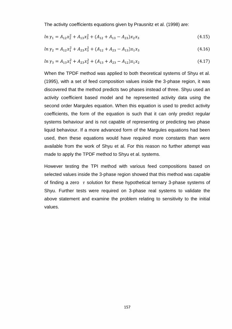
157
The activity coefficients equations given by Prausnitz et al. (1998) are:
𝑙𝑛 𝛾1 = 𝐴12𝑥22 + 𝐴13𝑥3
2 + (𝐴12 + 𝐴13 − 𝐴23)𝑥2𝑥3 (4.15)
𝑙𝑛 𝛾2 = 𝐴12𝑥12 + 𝐴23𝑥3
2 + (𝐴12 + 𝐴23 − 𝐴13)𝑥1𝑥3 (4.16)
𝑙𝑛 𝛾3 = 𝐴13𝑥12 + 𝐴23𝑥2
2 + (𝐴13 + 𝐴23 − 𝐴12)𝑥1𝑥2 (4.17)
When the TPDF method was applied to both theoretical systems of Shyu et al.
(1995), with a set of feed composition values inside the 3-phase region, it was
discovered that the method predicts two phases instead of three. Shyu used an
activity coefficient based model and he represented activity data using the
second order Margules equation. When this equation is used to predict activity
coefficients, the form of the equation is such that it can only predict regular
systems behaviour and is not capable of representing or predicting two phase
liquid behaviour. If a more advanced form of the Margules equations had been
used, then these equations would have required more constants than were
available from the work of Shyu et al. For this reason no further attempt was
made to apply the TPDF method to Shyu et al. systems.
However testing the TPI method with various feed compositions based on
selected values inside the 3-phase region showed that this method was capable
of finding a zero 𝜏 solution for these hypothetical ternary 3-phase systems of
Shyu. Further tests were required on 3-phase real systems to validate the
above statement and examine the problem relating to sensitivity to the initial
values.

158
Figure 4.19: A plot showing Gibbs energy surface and the tangent plane under the surface
for two ternary 3-phase systems of Shyu et al. (System 1 & System 2)
Figure 4.19 shows the Gibbs energy surface (𝜙) for the LLLE ternary artificial
systems of Shyu et al. (1995). Note that, in contrast to a binary, the 𝜙 curve is
now a surface in a 3 dimensional composition space. The tangent plane
(shaded triangle) lies under the Gibbs energy surface and the Global solution is

159
obtained when 𝜏 is zero. It is important to observe the difficulty of locating the
boundaries between these phases. The initialisation procedure used in the
binary system based on the location of phase boundaries is difficult to apply to
3-phase ternary systems. In the binary VLLE phase calculations for the majority
of the heterogeneous systems, the vapour phase lies between two other liquid
phases on the 𝜙 curve. Sometimes the location of the boundaries on the Gibbs
energy surface is not clearly defined, particularly in these types of LLLE
hypothetical mixtures and a mathematical approach to find the phase
boundaries is not available, especially when the activity coefficient model
(Margules) is used in describing the Gibbs energy surface.
In terms of applying the TPI and TPDF methods to real systems it should be
noted that Shyu only worked in theoretical phases and did not identify the
nature of the phase. The following work clearly works with vapour-liquid-liquid
systems.
160
4.6.2 The sensitivity of TPI method to initial values
One of the deficiencies of the TPI method when used in conjunction with the
Nelder-Mead simplex was found to be its sensitivity to the initial values. This
was found when applying the method to VLLE binary systems (Section
4.3.1).An Initial attempt to judge the effect of the starting values on the
performance of the TPI method on ternary VLLE data was carried out on three
ternary systems.
The TPI method was applied to the VLLE data for water(1)-acetone(2)-methyl
ethyl ketone(3) system [system 1] at 760 mmHg and six different temperatures
(range between 73.10 - 70.10 0C). The minimisation procedure (Nelder-Mead
simplex) allowed the adjustment of the six variables (𝛼𝑖, 𝜃𝑖) simultaneously.
The PRSV+WSMR was used to represent the Gibbs energy of the system
utilising the parameters obtained (table: 4.21) from 3-phase flash calculations.
This work has investigated the effect of different initial values on the
performance of the TPI method in ternary VLLE for the stated system. The initial
composition of the first component (water) is increased by (0.01 or 0.02)
increments whilst the second composition (acetone) is fixed at 0.01. This
scheme was applied to all the phases. Table (4.23) shows the initial values in
each phase at specified temperatures and the corresponding results of the TPI
method in absolute differences [𝛥𝑥𝑖 = |𝑥𝑖𝑒𝑥𝑝 − 𝑥𝑖
𝑝𝑟𝑒𝑑|], where 𝑒𝑥𝑝 is
experimental and 𝑝𝑟𝑒𝑑 is predicted using the TPI method. It can be seen from
table (4.23) that 10 different sets of initial values were used for each data point.
Observing the initial values used in table (4.23) and the final results of the TPI
method, it is obvious that if the initial values are closer to the actual solution the
differences, ∆𝑥𝑖 , are smaller and better results are produced. If the initial values
are not close to the actual solution the TPI simplex usually converges to an
incorrect solution for the stated physical conditions. The main reason for this
behaviour, as found by previous researchers(Hodges et al., 1998), is the
flattened shape of the (𝜙) surface around the solution compositions which
allows a zero 𝜏 solution to be obtained in areas which are significantly different
to the actual solution. Figure (4.20) shows the change of the 𝛥𝑥1 versus the
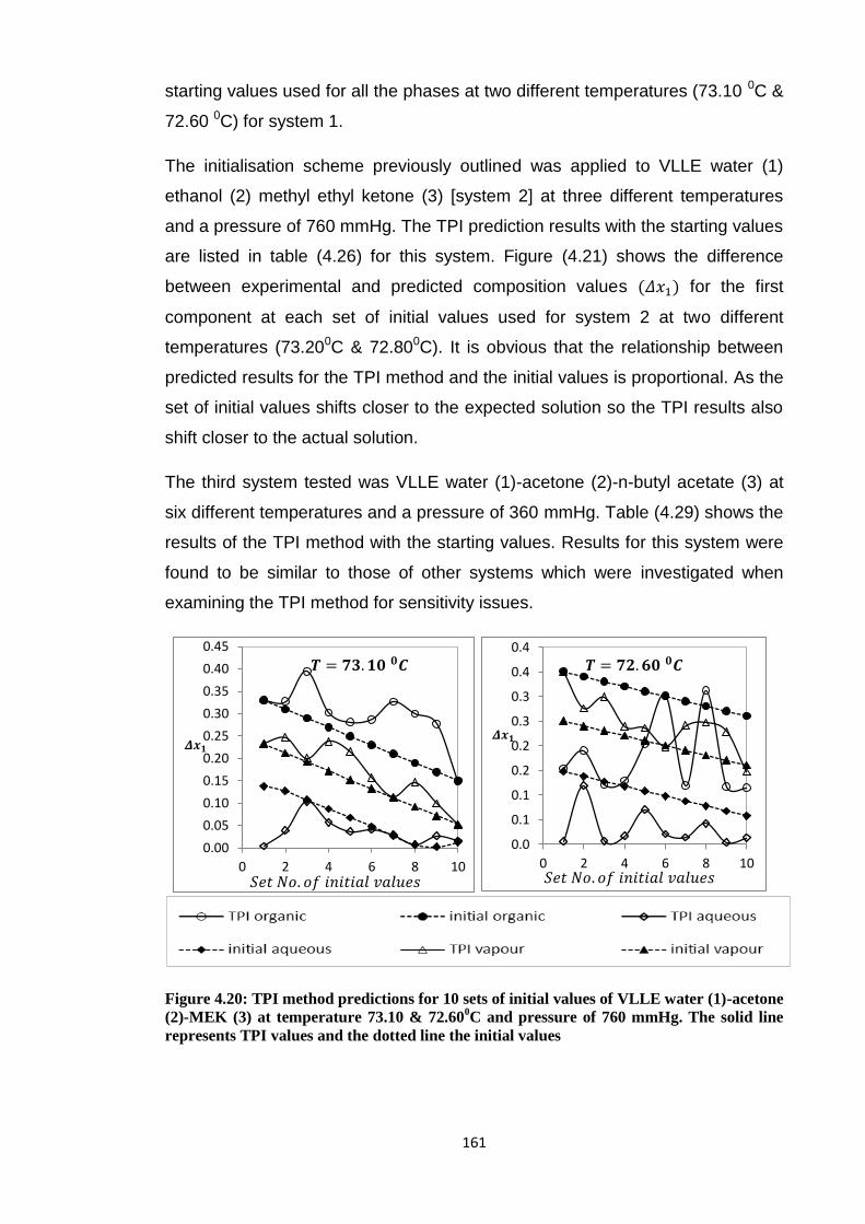
161
starting values used for all the phases at two different temperatures (73.10 0C &
72.60 0C) for system 1.
The initialisation scheme previously outlined was applied to VLLE water (1)
ethanol (2) methyl ethyl ketone (3) [system 2] at three different temperatures
and a pressure of 760 mmHg. The TPI prediction results with the starting values
are listed in table (4.26) for this system. Figure (4.21) shows the difference
between experimental and predicted composition values (𝛥𝑥1) for the first
component at each set of initial values used for system 2 at two different
temperatures (73.200C & 72.800C). It is obvious that the relationship between
predicted results for the TPI method and the initial values is proportional. As the
set of initial values shifts closer to the expected solution so the TPI results also
shift closer to the actual solution.
The third system tested was VLLE water (1)-acetone (2)-n-butyl acetate (3) at
six different temperatures and a pressure of 360 mmHg. Table (4.29) shows the
results of the TPI method with the starting values. Results for this system were
found to be similar to those of other systems which were investigated when
examining the TPI method for sensitivity issues.
Figure 4.20: TPI method predictions for 10 sets of initial values of VLLE water (1)-acetone
(2)-MEK (3) at temperature 73.10 & 72.600C and pressure of 760 mmHg. The solid line
represents TPI values and the dotted line the initial values
0.00
0.05
0.10
0.15
0.20
0.25
0.30
0.35
0.40
0.45
0 2 4 6 8 10𝑆𝑒𝑡 𝑁𝑜. 𝑜𝑓 𝑖𝑛𝑖𝑡𝑖𝑎𝑙 𝑣𝑎𝑙𝑢𝑒𝑠
𝜟𝒙𝟏
𝑻 = 𝟕𝟑. 𝟏𝟎 𝟎𝑪
0.0
0.1
0.1
0.2
0.2
0.3
0.3
0.4
0.4
0 2 4 6 8 10𝑆𝑒𝑡 𝑁𝑜. 𝑜𝑓 𝑖𝑛𝑖𝑡𝑖𝑎𝑙 𝑣𝑎𝑙𝑢𝑒𝑠
𝜟𝒙𝟏
𝑻 = 𝟕𝟐. 𝟔𝟎 𝟎𝑪
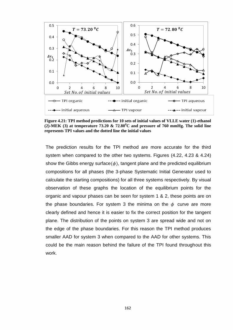
162
Figure 4.21: TPI method predictions for 10 sets of initial values of VLLE water (1)-ethanol
(2)-MEK (3) at temperature 73.20 & 72.800C and pressure of 760 mmHg. The solid line
represents TPI values and the dotted line the initial values
The prediction results for the TPI method are more accurate for the third
system when compared to the other two systems. Figures (4.22, 4.23 & 4.24)
show the Gibbs energy surface(𝜙), tangent plane and the predicted equilibrium
compositions for all phases (the 3-phase Systematic Initial Generator used to
calculate the starting compositions) for all three systems respectively. By visual
observation of these graphs the location of the equilibrium points for the
organic and vapour phases can be seen for system 1 & 2, these points are on
the phase boundaries. For system 3 the minima on the 𝜙 curve are more
clearly defined and hence it is easier to fix the correct position for the tangent
plane. The distribution of the points on system 3 are spread wide and not on
the edge of the phase boundaries. For this reason the TPI method produces
smaller AAD for system 3 when compared to the AAD for other systems. This
could be the main reason behind the failure of the TPI found throughout this
work.
0.0
0.1
0.2
0.3
0.4
0.5
0 2 4 6 8 10
𝑻 = 𝟕𝟑. 𝟐𝟎 𝟎𝑪
𝜟𝒙𝟏
𝑆𝑒𝑡 𝑁𝑜. 𝑜𝑓 𝑖𝑛𝑖𝑡𝑖𝑎𝑙 𝑣𝑎𝑙𝑢𝑒𝑠
0.0
0.1
0.2
0.3
0.4
0.5
0.6
0 2 4 6 8 10
𝑻 = 𝟕𝟐. 𝟖𝟎 𝟎𝑪
𝑆𝑒𝑡 𝑁𝑜. 𝑜𝑓 𝑖𝑛𝑖𝑡𝑖𝑎𝑙 𝑣𝑎𝑙𝑢𝑒𝑠
𝜟𝒙𝟏
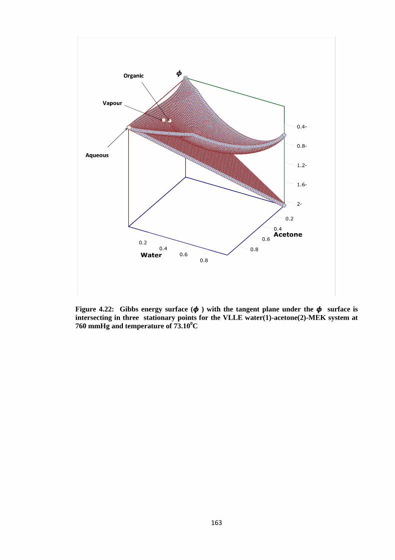
163
Figure 4.22: Gibbs energy surface (𝝓 ) with the tangent plane under the 𝝓 surface is
intersecting in three stationary points for the VLLE water(1)-acetone(2)-MEK system at
760 mmHg and temperature of 73.100C

164
Figure 4.23: Gibbs energy surface (𝝓 ) with the tangent plane under the 𝝓 surface is
intersecting in three stationary points, for the VLLE water(1)-ethanol(2)-MEK system at
760 mmHg and temperature of 73.200C
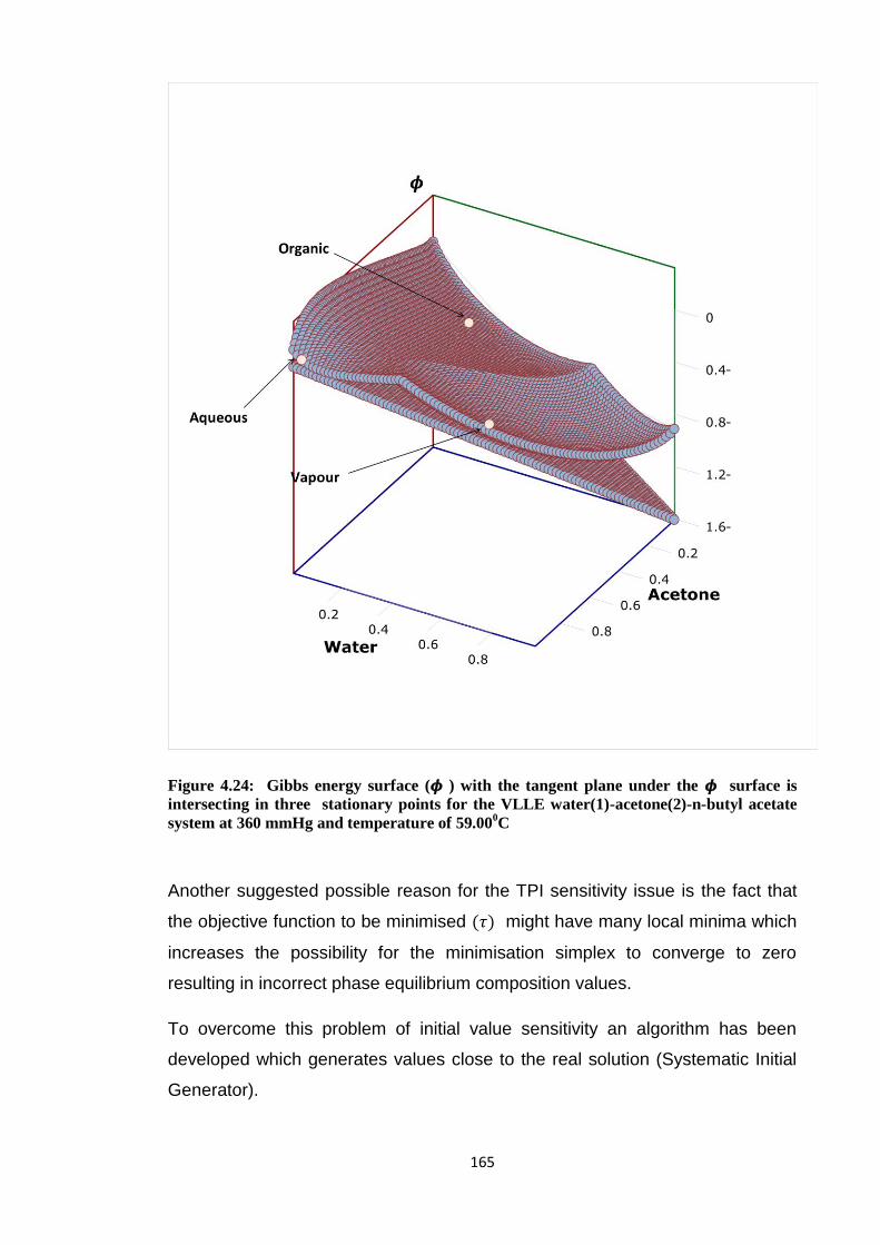
165
Figure 4.24: Gibbs energy surface (𝝓 ) with the tangent plane under the 𝝓 surface is
intersecting in three stationary points for the VLLE water(1)-acetone(2)-n-butyl acetate
system at 360 mmHg and temperature of 59.000C
Another suggested possible reason for the TPI sensitivity issue is the fact that
the objective function to be minimised (𝜏) might have many local minima which
increases the possibility for the minimisation simplex to converge to zero
resulting in incorrect phase equilibrium composition values.
To overcome this problem of initial value sensitivity an algorithm has been
developed which generates values close to the real solution (Systematic Initial
Generator).
166
4.6.3 Systematic Initial Generator (SIG)
The sensitivity of the TPI method to initial values is due to the method of
formulating this mathematical problem (Gibbs energy minimisation).The main
idea of the TPI method suggested by Hodges et al. (1998) is the calculation and
minimisation of a hyper-tangent plane that is bounded by Gibbs energy surface
quantity (𝜏) via the repeated search of a tangent distance function 𝐹(𝑥) value
to adjust the tangent position in relation to the (𝜙) surface.
In the literature survey section (2.5), it is clearly outlined that in Gibbs
minimisation methods of phase equilibrium calculations there is a possibility for
the optimisation to converge to a trivial or local rather than a global solution,
when a poor initial estimate is supplied. Many researchers have related this
problem to the non-convex non-linear properties of the objective function with
several local minima. The survey also concluded that the methods and
strategies selected depend on the type of phase calculations (LLE, VLE, and
VLLE), complexity of the systems (level of non-ideality) and the operating
conditions (temperature and pressure).
In phase equilibrium calculations on VLE hydrocarbon systems at low and
moderate pressures, Michelsen (1982 b) used two sets of initial estimates which
are calculated from a relative volatility (K-factor) expression using the Wilson
correlation. (See literature survey section (2.5.1)). This initial estimation is
based on the critical pressure, critical temperature and acentric factor for pure
component at the system temperature. Other researchers suggested a different
initialisation scheme for the LLE calculation on ternary systems; however the
initialisation scheme for VLLE multi-component calculations for the polar non-
ideal systems of interest has not been thoroughly investigated.
Some of the initialisation methods rely on a 2 phase stability test and phase split
as an initial estimate for 3 phase calculations; however the direct initialisation
method for VLLE multicomponent heterogeneous systems (in particular the
systems investigated in this work) is not covered in the literature. For this
reason and in an attempt to improve the reliability of the TPI method for 3-phase
calculations of ternary systems, this work suggests and applies a direct
initialisation algorithm for VLLE multicomponent systems. The details of the
167
suggested method of initialisation can be found in the theory section (3.11.2).
This work has adopted the VLLE initialisation method for 3-phase flash
calculations. This method combines the LLE and VLE initialisation strategies
using UNIQUAC as an activity coefficient model, PRSV+WSMR as EOS and
the Rachford-Rice equation as a 3-phase flash calculation. The main objective
function in the algorithm minimises relative volatilities of the component in the
mixture.
The initialisation method developed in this work was applied to the VLLE ternary
data for the systems listed at the beginning of this section. The systematic initial
values have a positive effect on the final results for the TPI method. The SIG
apparently supplies the TPI method with more realistic and logical starting
values.
The effect of SIG can be seen for system 1: water (1)-acetone (2)-MEK (3) at
760 mmHg; when the results for the TPI method (𝛥𝑥𝑖) in table (4.22) are
compared to (𝛥𝑥𝑖) in table (4.23). The prediction results for the TPI method with
embedded SIG are significantly improved if compared to the results when
arbitrary initial values are used. This statement can be applied to the other
systems investigated. Tables (4.25, 4.26) and (4.28, 4.29) show the results for
system 2: water (1)-ethanol (2)-MEK (3) at 760 mmHg and system 3: water (1)-
acetone (2) - n-butyl acetate (3) at pressure of 360 mmHg respectively.
This section shows that the accuracy of the final prediction results for the TPI
method strongly depends on initial estimates. This has been demonstrated
when a number of sets of initial values were tested using the TPI method on
three VLLE ternary systems at different temperatures. At each temperature data
point 10 sets of initial values were used to measure the sensitivity of the TPI
method. The effects of the Systematic Initial Generator on the final results of the
TPI method have been demonstrated.
This research has also examined another Gibbs minimisation method
suggested by Michelsen known as Tangent Plane Distance Function (TPDF).
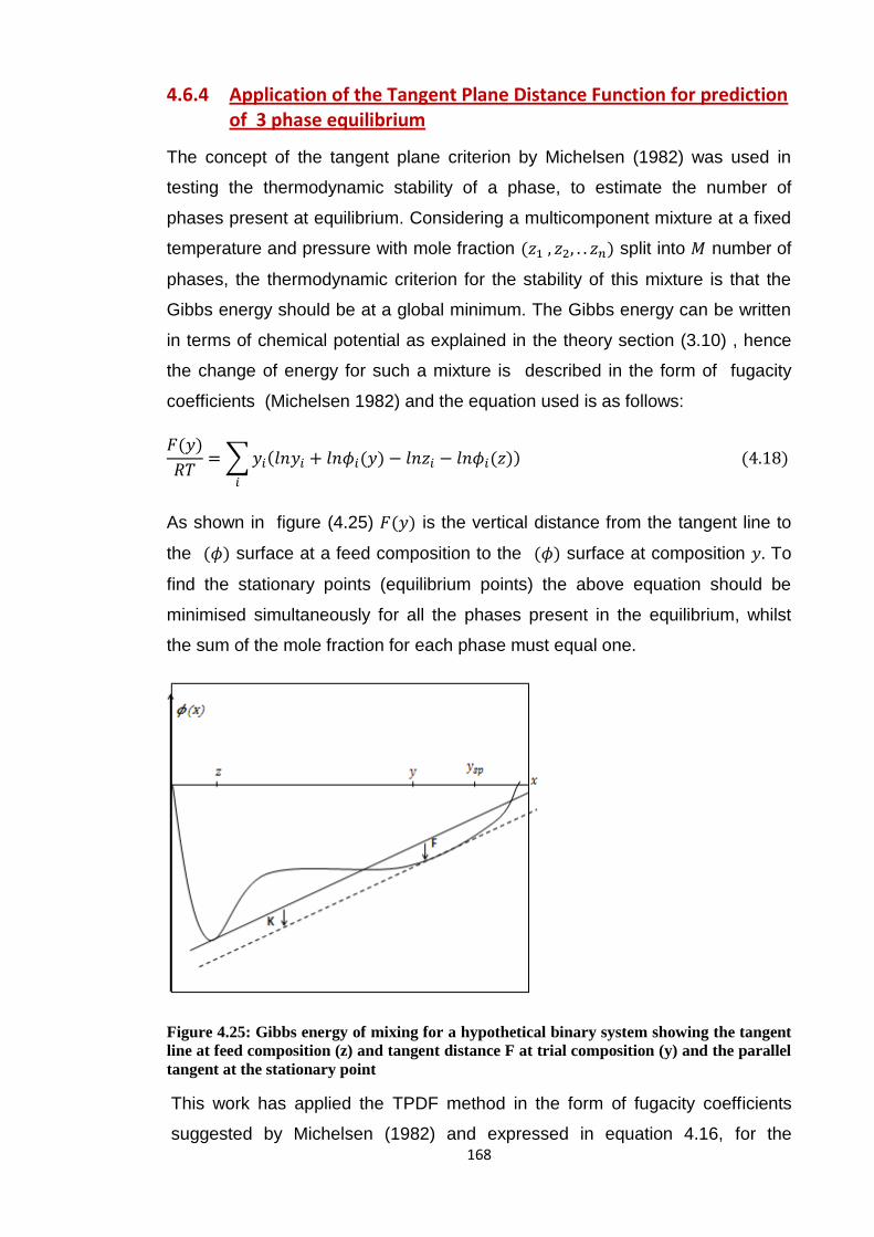
168
4.6.4 Application of the Tangent Plane Distance Function for prediction of 3 phase equilibrium
The concept of the tangent plane criterion by Michelsen (1982) was used in
testing the thermodynamic stability of a phase, to estimate the number of
phases present at equilibrium. Considering a multicomponent mixture at a fixed
temperature and pressure with mole fraction (𝑧1 , 𝑧2, . . 𝑧𝑛) split into 𝑀 number of
phases, the thermodynamic criterion for the stability of this mixture is that the
Gibbs energy should be at a global minimum. The Gibbs energy can be written
in terms of chemical potential as explained in the theory section (3.10) , hence
the change of energy for such a mixture is described in the form of fugacity
coefficients (Michelsen 1982) and the equation used is as follows:
𝐹(𝑦)
𝑅𝑇= ∑ 𝑦𝑖(𝑙𝑛𝑦𝑖 + 𝑙𝑛𝜙𝑖(𝑦) − 𝑙𝑛𝑧𝑖 − 𝑙𝑛𝜙𝑖(𝑧))
𝑖
(4.18)
As shown in figure (4.25) 𝐹(𝑦) is the vertical distance from the tangent line to
the (𝜙) surface at a feed composition to the (𝜙) surface at composition 𝑦. To
find the stationary points (equilibrium points) the above equation should be
minimised simultaneously for all the phases present in the equilibrium, whilst
the sum of the mole fraction for each phase must equal one.
Figure 4.25: Gibbs energy of mixing for a hypothetical binary system showing the tangent
line at feed composition (z) and tangent distance F at trial composition (y) and the parallel
tangent at the stationary point
This work has applied the TPDF method in the form of fugacity coefficients
suggested by Michelsen (1982) and expressed in equation 4.16, for the

169
prediction of VLLE for all the ternary systems previously cited. The TPDF
method was tested for sensitivity issues and the same initial values used for
the TPI were also used here.
The subsequent results were compared with the TPI method. Tables (4.23,
4.26 and 4.29) show the TPI and the TPDF results for three VLLE systems
investigated. These tables show at each temperature a set of 10 different initial
values used and the [𝛥𝑥𝑖 = |𝑥𝑖𝑒𝑥𝑝 − 𝑥𝑖
𝑝𝑟𝑒𝑑|] calculated from the predictions
using both methods.
Analysis of these tables shows that the TPDF predictions give consistently
more satisfactory results when compared to the TPI method which produces
significantly less accurate results. The Absolute Average Deviation (AAD) was
0.004 from the experimental data for the water (1) acetone (2)-MEK (3) [system
1] compared to an AAD for the TPI method of 0.128. The results for system1
are presented in table (4.23). The TPDF predictions for VLLE water (1)-ethanol
(2)-methyl ethyl ketone (3) [system 2] at 760 mmHg can be seen in table (4.26)
and the AAD for this system is 0.01, compared to an AAD of the TPI of 0.175
for the same system. Table (4.29) contains the TPDF and the TPI results for
VLLE water (1) acetone (2)-n-butyl acetate (3) [system 3] at 360 mmHg and the
AAD for all data points is 0.017 and 0.096 for TPDF and TPI respectively. It can
be seen that the AAD values produced by both methods are relatively low. This
is consistent with the nature of the 𝜙 surface for the systems which have been
discussed previously. The AAD values for the three systems studied indicate
that the TPDF method is more effective than the TPI method in prediction of
phase equilibrium compositions for heterogeneous high polar systems based
on the known experimental data. In addition a positive feature of the TPDF
method is it is less sensitive to the initial values which make this method
efficient and reliable in the prediction of phase equilibria.
170
4.6.5 The SIG ,TPI and TPDF as Phase predictors
The TPI, TPDF and SIG were tested on the four ternary VLLE systems of
Younis et al. (2007) at a specific temperature and at a system pressure with
different sets of overall feed composition outside the 3-phase region. The TPI
initial starting values were obtained from SIG results. The results for these
methods as phase predictor for four systems are shown: in table (4.24) for
water (1)-acetone (2)-MEK (3) at pressure of 760 mmHg, in table (4.27) for
water (1)-ethanol (2)-MEK (3) at pressure of 760 mmHg, in tables: (4.30,4.32
and 4.34) for water (1)-acetone (2)-n-butyl acetate (3) at pressures of 360, 600
and 760 mmHg respectively and in tables (4.36, 4.38 and 4.40) for water (1)-
ethanol (2)-n-butyl acetate (3) at pressures of 360, 600 and 760 mmHg
respectively.
The results indicate that the SIG and TPDF methods can predict the number of
phases when the feed composition is outside the 3-Phase region (by producing
the single liquid phase composition). However the TPI is not capable of
identifying the 2-phase region even though the TPI starting values were
obtained from the SIG which had already indicated the 2-phase region. The
reason for the failure of the TPI to predict the correct number of phases is due
to the search pattern of the TPI algorithm using the angle variable (𝜃𝑖) which is
related to the length variable(𝛼𝑖). Each angle is related to a phase which rotates
between (0 - 360) degrees and for the TPI to converge to a 3-phase solution
each angle has to be constrained in a range of values dependant on the prior
knowledge of the heterogeneous system whilst the (𝛼𝑖) values were
constrained between (0 -1).
The TPDF method was used as a phase predictor by testing a number of sets
of values of feed compositions outside the 3-phase region. The results indicate
a single liquid phase with compositions which differ from the feed composition
values for both of these systems of water-acetone-n-butyl acetate and water-
ethanol-n-butyl acetate. However the TPDF method displayed unpredictable
behaviour only outside the 3-phase region for the two systems water-acetone-
MEK and water-ethanol-MEK. The values of the single liquid phase results were
the same as the feed compositions. When an attempt at convergence for this
method was further explored it was found that the method pushed the initial

171
values to a range of different values but for these systems the values always
returned to the feed composition values initially supplied. It should be noted that
this behaviour was not observed for systems containing water-n-butyl acetate,
for these systems the TPDF method converged to results correctly predicting
the phases present.
For the systems containing the water-MEK binary, the TPDF method was
capable of correct phase predictions when the initial feed compositions lay
within the heterogeneous region. The problem with this system only arose when
the initial values lay outside the known heterogeneous region. It appears that
the representation of the 𝜙 curve for systems containing the MEK-water binary
is of such a nature that the TPDF method is not able to easily recognise the
phase boundaries. This aspect of these systems requires further research and
analysis.
A sub-procedure was developed based on minimisation of relative volatility
values ( 𝐾𝑖) in the Flash calculation. The values of phase compositions of the
TPDF method were used as initial values for this calculation and the 𝐾𝑖 are
calculated and stored. The fractions of molar rate of organic and aqueous liquid
phases were calculated in an internal loop then the new values of 𝐾𝑖 were
calculated and compared with the stored values |𝐾𝑖𝑜𝑙𝑑 − 𝐾𝑖
𝑛𝑒𝑤| and the value
(10-5) of the absolute difference was used as the stopping condition. The use of
the additional sub-procedure has improved the reliability of the TPDF as a
phase predictor.
4.6.6 The Flash ,TPI and TPDF Phase Equilibrium results
The VLLE flash calculation was applied to the ternary systems of interest and
the parameters obtained were used in the SIG, TPI and TPDF prediction
methods for VLLE phase equilibrium calculations. A set of feed compositions
were chosen inside the 3-Phase heterogeneous region for each experimental
temperature which lies on the experimental tie line. The results of the Flash ,
TPI and TPDF for these ternary systems can be found in: table (4.22) for water
(1)-acetone (2)-MEK (3) at pressure of 760 mmHg , table (4.25) for water (1)-
ethanol (2)-MEK (3) at pressure of 760 mmHg ,tables (4.28,4.31 and 4.33) for
water (1)-acetone (2)-n-butyl acetate(3) at pressures of 360, 600 760 mmHg
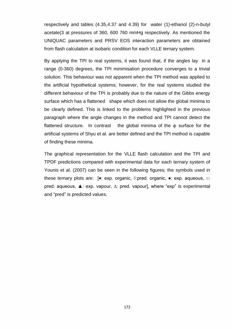
172
respectively and tables (4.35,4.37 and 4.39) for water (1)-ethanol (2)-n-butyl
acetate(3 at pressures of 360, 600 760 mmHg respectively. As mentioned the
UNIQUAC parameters and PRSV EOS interaction parameters are obtained
from flash calculation at isobaric condition for each VLLE ternary system.
By applying the TPI to real systems, it was found that, if the angles lay in a
range (0-360) degrees, the TPI minimisation procedure converges to a trivial
solution. This behaviour was not apparent when the TPI method was applied to
the artificial hypothetical systems; however, for the real systems studied the
different behaviour of the TPI is probably due to the nature of the Gibbs energy
surface which has a flattened shape which does not allow the global minima to
be clearly defined. This is linked to the problems highlighted in the previous
paragraph where the angle changes in the method and TPI cannot detect the
flattened structure. In contrast the global minima of the ϕ surface for the
artificial systems of Shyu et al. are better defined and the TPI method is capable
of finding these minima.
The graphical representation for the VLLE flash calculation and the TPI and
TPDF predictions compared with experimental data for each ternary system of
Younis et al. (2007) can be seen in the following figures; the symbols used in
these ternary plots are: [♦: exp. organic, ◊:pred. organic, ●: exp. aqueous, ○:
pred. aqueous, ▲: exp. vapour, ∆: pred. vapour], where “exp” is experimental
and “pred” is predicted values.
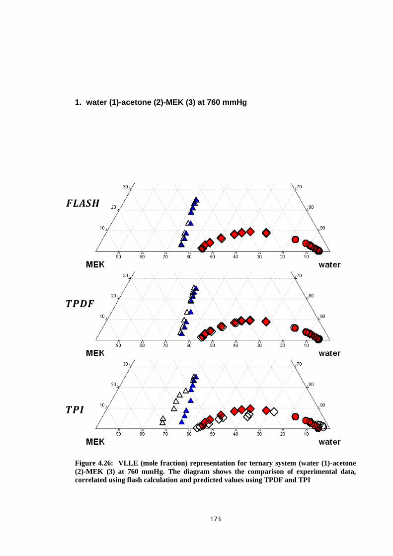
173
1. water (1)-acetone (2)-MEK (3) at 760 mmHg
Figure 4.26: VLLE (mole fraction) representation for ternary system (water (1)-acetone
(2)-MEK (3) at 760 mmHg. The diagram shows the comparison of experimental data,
correlated using flash calculation and predicted values using TPDF and TPI
𝑭𝑳𝑨𝑺𝑯
𝑻𝑷𝑫𝑭
𝑻𝑷𝑰

174
2. water (1)-acetone (2)-MEK (3) at 760 mmHg
Figure 4.27: VLLE (mole fraction) representation for ternary system (water (1)-ethanol
(2)-MEK (3) at 760 mmHg. The diagram shows the comparison of experimental data,
correlated using flash calculation and predicted values using TPDF and TPI
3. water (1)-acetone (2)-n-butyl acetate(3)
The flash calculation, the TPI and TPDF results for the third system VLLE
water (1) – acetone (2)-n-butyl acetate (3) at pressure 360, 600 and 760 mmHg
are listed in tables (4.28, 4.31 and 4.33) respectively. Figures 4.28 through
4.36 below present the graphical representation for calculated results using the
3-phase flash calculation values, the predicted composition values for the TPDF
and the TPI respectively.
FLASH
TPD
TPI
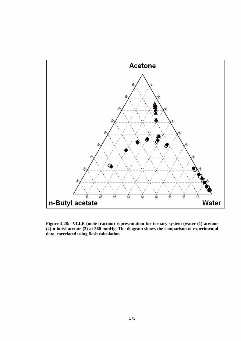
175
Figure 4.28: VLLE (mole fraction) representation for ternary system (water (1)-acetone
(2)-n-butyl acetate (3) at 360 mmHg. The diagram shows the comparison of experimental
data, correlated using flash calculation
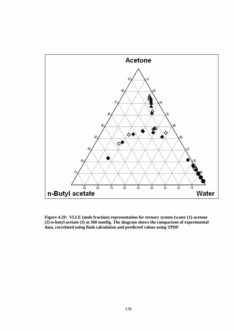
176
Figure 4.29: VLLE (mole fraction) representation for ternary system (water (1)-acetone
(2)-n-butyl acetate (3) at 360 mmHg. The diagram shows the comparison of experimental
data, correlated using flash calculation and predicted values using TPDF
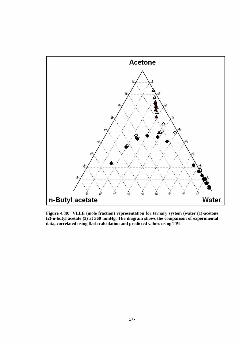
177
Figure 4.30: VLLE (mole fraction) representation for ternary system (water (1)-acetone
(2)-n-butyl acetate (3) at 360 mmHg. The diagram shows the comparison of experimental
data, correlated using flash calculation and predicted values using TPI

178
Figure 4.31: VLLE (mole fraction) representation for ternary system (water (1)-acetone
(2)-n-butyl acetate (3) at 600 mmHg. The diagram shows the comparison of experimental
data, correlated using flash calculation
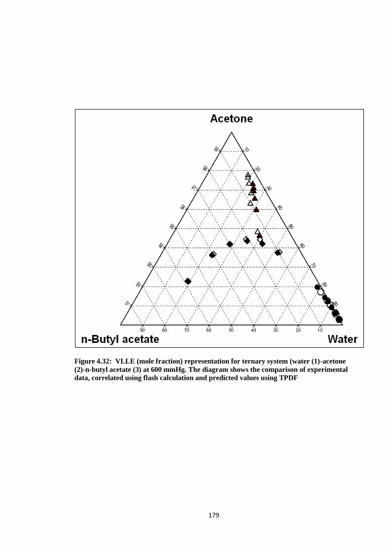
179
Figure 4.32: VLLE (mole fraction) representation for ternary system (water (1)-acetone
(2)-n-butyl acetate (3) at 600 mmHg. The diagram shows the comparison of experimental
data, correlated using flash calculation and predicted values using TPDF
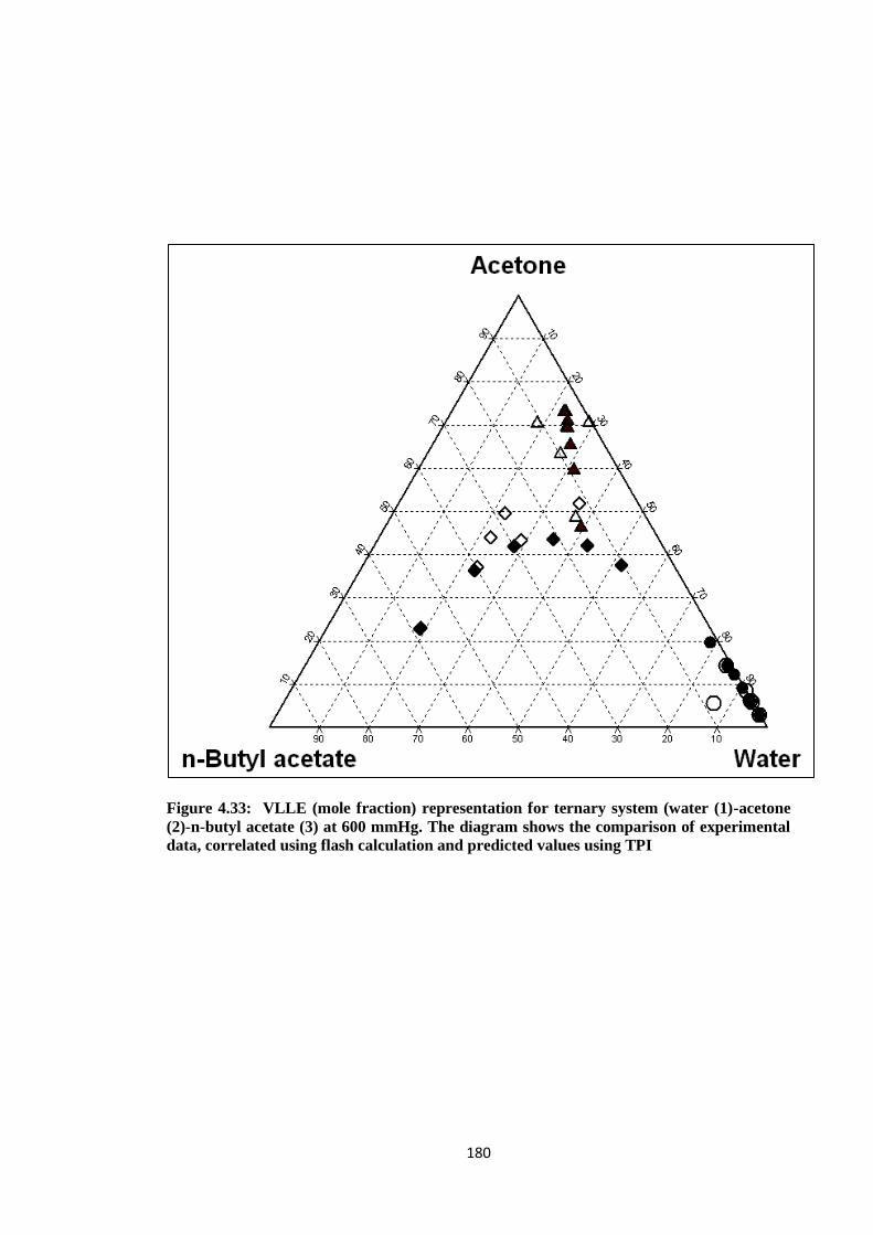
180
Figure 4.33: VLLE (mole fraction) representation for ternary system (water (1)-acetone
(2)-n-butyl acetate (3) at 600 mmHg. The diagram shows the comparison of experimental
data, correlated using flash calculation and predicted values using TPI

181
Figure 4.34: VLLE (mole fraction) representation for ternary system (water (1)-acetone
(2)-n-butyl acetate (3) at 760 mmHg. The diagram shows the comparison of experimental
data, correlated using flash calculation

182
Figure 4.35: VLLE (mole fraction) representation for ternary system (water (1)-acetone
(2)-n-butyl acetate (3) at 760 mmHg. The diagram shows the comparison of experimental
data , correlated using flash calculation and predicted values using TPDF

183
Figure 4.36: VLLE (mole fraction) representation for ternary system (water (1)-acetone
(2)-n-butyl acetate (3) at 760 mmHg. The diagram shows the comparison of experimental
data, correlated using flash calculation and predicted values using TPI
4. water (1)-ethanol (2)-n-butyl acetate(3)
The flash calculation, the TPI and TPDF results for the third system VLLE water
(1) – ethanol (2)-n-butyl acetate (3) at pressure 360, 600 and 760 mmHg are
listed in table (4.35, 4.37 and 4.39) respectively. Figures (4.37, 4.38 & 4.39)
below present the graphical representation for calculated results using the 3-
phase flash calculation, the predicted composition values for the TPDF and the
TPI respectively.
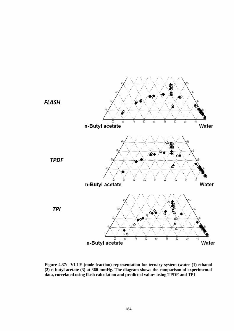
184
Figure 4.37: VLLE (mole fraction) representation for ternary system (water (1)-ethanol
(2)-n-butyl acetate (3) at 360 mmHg. The diagram shows the comparison of experimental
data, correlated using flash calculation and predicted values using TPDF and TPI
FLASH
TPDF
TPI
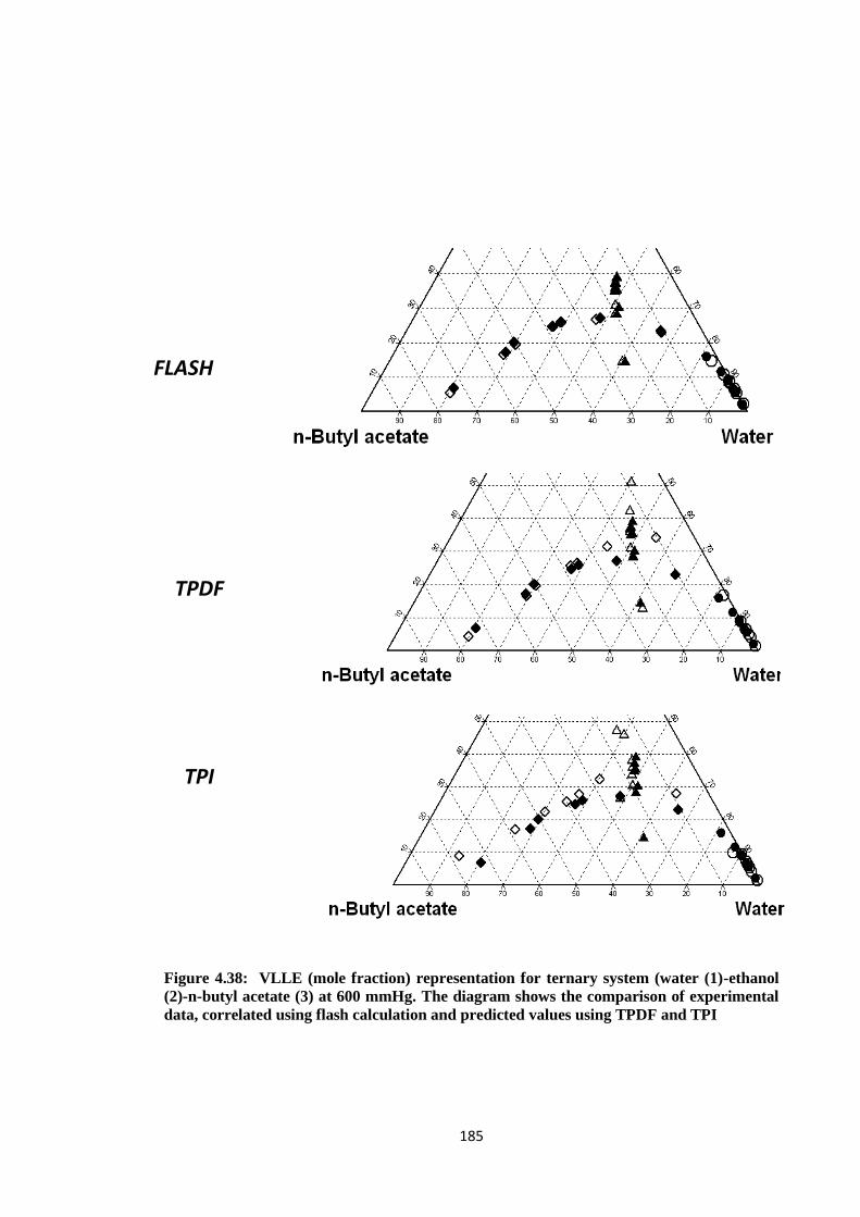
185
Figure 4.38: VLLE (mole fraction) representation for ternary system (water (1)-ethanol
(2)-n-butyl acetate (3) at 600 mmHg. The diagram shows the comparison of experimental
data, correlated using flash calculation and predicted values using TPDF and TPI
FLASH
TPDF
TPI

186
Figure 4.39: VLLE (mole fraction) representation for ternary system (water (1)-ethanol
(2)-n-butyl acetate (3) at 760 mmHg. The diagram shows the comparison of experimental
data, correlated using flash calculation and predicted values using TPDF and TPI
FLASH
TPDF
TPI
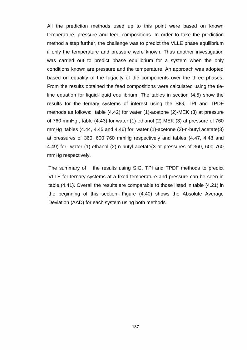
187
All the prediction methods used up to this point were based on known
temperature, pressure and feed compositions. In order to take the prediction
method a step further, the challenge was to predict the VLLE phase equilibrium
if only the temperature and pressure were known. Thus another investigation
was carried out to predict phase equilibrium for a system when the only
conditions known are pressure and the temperature. An approach was adopted
based on equality of the fugacity of the components over the three phases.
From the results obtained the feed compositions were calculated using the tie-
line equation for liquid-liquid equilibrium. The tables in section (4.5) show the
results for the ternary systems of interest using the SIG, TPI and TPDF
methods as follows: table (4.42) for water (1)-acetone (2)-MEK (3) at pressure
of 760 mmHg , table (4.43) for water (1)-ethanol (2)-MEK (3) at pressure of 760
mmHg ,tables (4.44, 4.45 and 4.46) for water (1)-acetone (2)-n-butyl acetate(3)
at pressures of 360, 600 760 mmHg respectively and tables (4.47, 4.48 and
4.49) for water (1)-ethanol (2)-n-butyl acetate(3 at pressures of 360, 600 760
mmHg respectively.
The summary of the results using SIG, TPI and TPDF methods to predict
VLLE for ternary systems at a fixed temperature and pressure can be seen in
table (4.41). Overall the results are comparable to those listed in table (4.21) in
the beginning of this section. Figure (4.40) shows the Absolute Average
Deviation (AAD) for each system using both methods.

188
Figure 4.40: AAD for VLLE predictions for ternary systems showing the TPI and TPDF
methods where TPI-1 and TPDF-1 indicates that the predicted values obtained at known
temperature , pressure and feed compositions , TPI-2 and TPDF-2 indicates that the
prediction values are obtained from knowing temperature and pressure of the system
0.000
0.005
0.010
0.015
0.020
0.025
0.030
0.035
0.040
0.045
0.050
0 1 2 3 4 5 6 7 8 9
TPDF-1
TPDF-2
AAD
System No.
0.00
0.02
0.04
0.06
0.08
0.10
0.12
0.14
0.16
0 1 2 3 4 5 6 7 8 9
TPI-1
TPI-2AAD
System No.
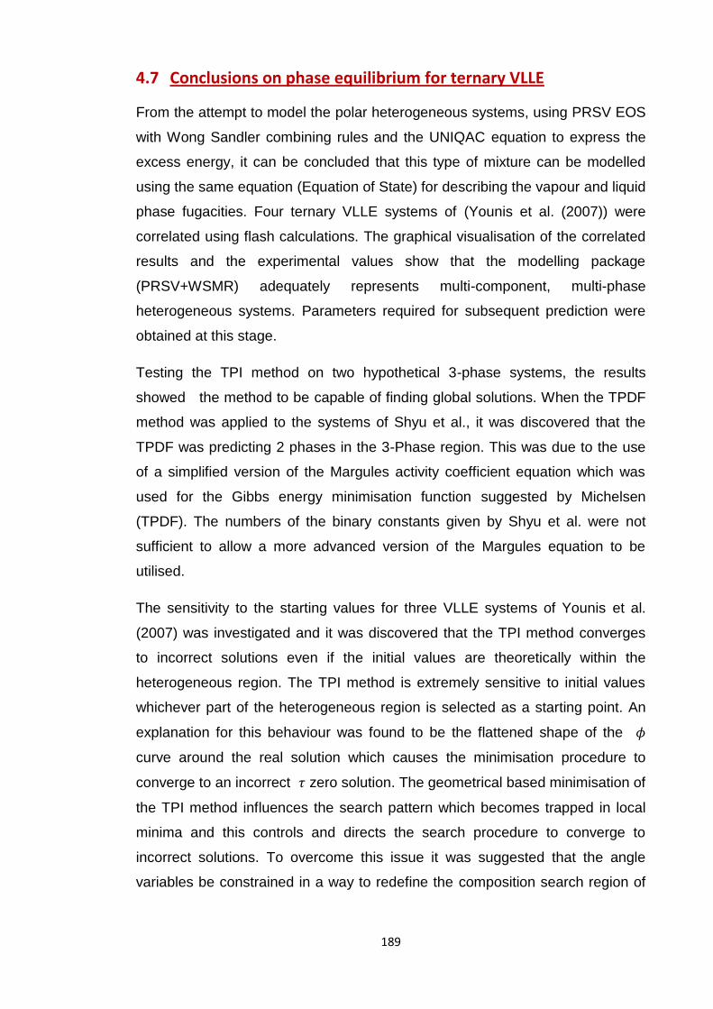
189
4.7 Conclusions on phase equilibrium for ternary VLLE
From the attempt to model the polar heterogeneous systems, using PRSV EOS
with Wong Sandler combining rules and the UNIQAC equation to express the
excess energy, it can be concluded that this type of mixture can be modelled
using the same equation (Equation of State) for describing the vapour and liquid
phase fugacities. Four ternary VLLE systems of (Younis et al. (2007)) were
correlated using flash calculations. The graphical visualisation of the correlated
results and the experimental values show that the modelling package
(PRSV+WSMR) adequately represents multi-component, multi-phase
heterogeneous systems. Parameters required for subsequent prediction were
obtained at this stage.
Testing the TPI method on two hypothetical 3-phase systems, the results
showed the method to be capable of finding global solutions. When the TPDF
method was applied to the systems of Shyu et al., it was discovered that the
TPDF was predicting 2 phases in the 3-Phase region. This was due to the use
of a simplified version of the Margules activity coefficient equation which was
used for the Gibbs energy minimisation function suggested by Michelsen
(TPDF). The numbers of the binary constants given by Shyu et al. were not
sufficient to allow a more advanced version of the Margules equation to be
utilised.
The sensitivity to the starting values for three VLLE systems of Younis et al.
(2007) was investigated and it was discovered that the TPI method converges
to incorrect solutions even if the initial values are theoretically within the
heterogeneous region. The TPI method is extremely sensitive to initial values
whichever part of the heterogeneous region is selected as a starting point. An
explanation for this behaviour was found to be the flattened shape of the 𝜙
curve around the real solution which causes the minimisation procedure to
converge to an incorrect 𝜏 zero solution. The geometrical based minimisation of
the TPI method influences the search pattern which becomes trapped in local
minima and this controls and directs the search procedure to converge to
incorrect solutions. To overcome this issue it was suggested that the angle
variables be constrained in a way to redefine the composition search region of
190
each phase in the minimisation to avoid the convergence to a local minima.
This was found to be effective and improved the results for the TPI method.
A further contributing factor to the TPI sensitivity issue is the location of the
stationary equilibrium points relative to the phase boundaries. The graphical
representation for the Gibbs energy surface for system 1 & 2 of Younis et al.
(2007) showed the stationary points for the organic and vapour phase
compositions to be on the phase boundaries (ternary systems which have
MEK). By contrast, for system 3 these points are relatively far apart on the 𝜙
surface.
In an attempt to provide the TPI minimisation method simplex with realistic initial
values, this research suggested a Systematic Initial Generator (SIG) as a direct
initialisation scheme for VLLE multi-component systems. The SIG method was
tested on four VLLE ternary systems and it has been demonstrated that this
method produces an overall improvement in the TPI results.
The differences between the two methods of Gibbs minimisation techniques
(TPI & TPDF) have been discussed. Both methods represent the
thermodynamic criterion aspect for equilibrium by constructing an objective
function to be minimised, but each method uses a different mathematical
approach. The TPI method converts the problem to a geometrical shape
through construction of the 𝜙 curve and tangent hyper-plane. The search
procedure finds the location of the tangent hyper-plane in relation to the 𝜙
surface. When the tangent is located under the 𝜙 surface a part of the tangent
which intersects with the 𝜙 will be reduced to zero.
Alternatively the TPDF method formulates the problem mathematically by
minimising the Gibbs energy of the mixture expressed in the form of fugacity
coefficients. This approach was developed by Michelsen (1982a) and was
essentially derived from chemical potential criteria. The function is expressed in
the form of the differences between the 𝜙 surface and the two parallel tangent
hyper planes at feed compositions and at trial compositions. The solution for
these rigorous mathematical problems is to minimise these differences with the
constraint that the sum of the compositions in each phase must be equal to one.
The results are the compositions of the stationary points for all phases.

191
From the analytical observation of both methods, the TPDF method apparently
has less local minima which allow the minimisation to converge to solutions with
less computational effort. A further advantage of the TPDF method is that it
can be applied to quaternary systems without any major change in the method
when compared to the TPI method. The TPDF method is robust and reliable
and can usually be applied successfully to systems of interest without showing
inconsistency and sensitivity to the initial values for the simplex.
The SIG, TPI and TPDF methods were investigated as phase predictors on the
systems of Younis et al (2007). A set of feed compositions were selected
outside the heterogeneous region. The results for SIG and TPDF methods
correctly indicated when the system forms a single liquid phase at a fixed
temperature and pressure. However the TPI results indicated that for the same
feed compositions the liquid splits into two phases when in fact only a single
liquid phase is present.
Applying the TPI to quaternary 3 phase systems introduces an extra degree of
freedom to the system according to phase rule and increases the total number
of variable compositions from 6 to 8. The base-case calculation is required to
calculate the global solution which splits into two ternary pseudo systems and
two hyper planes to be adjusted simultaneously as the Gibbs energy only exists
in a 3-dimensionl space. This increases the complexity of the method and also
increases the sensitivity to the initial values to start the simplex. For this reason
the TPI is only applied to VLLE ternary systems.
Overall, for ternary systems, this work has demonstrated that the PRSV
equation of state with WS mixing rules is capable of satisfactorily correlating
real heterogeneous system data. When attempting to use the Tangent Plane
Intersection (TPI) and the Tangent Plane Distance Function (TPDF) method it
has been demonstrated that, for four heterogeneous VLLE systems these
methods give variable prediction results. Usually the TPDF method is capable
of accurate predictions inside and outside the heterogeneous regions. The
behaviour of the TPI method was much more variable. This method is also
sensitive to the initial starting values supplied to the simplex method. Attempts
were carried out to supply more realistic starting values. The details of these
findings have been given in this conclusion section.

192
4.8 Quaternary systems
The correlation and predictions for two quaternary VLLE systems were carried
out using data published by Younis et al. (2007). The methods used were:
1. Flash calculation
2. Tangent Plane Distance Function (TPDF)
3. Systematic Initial Generator(SIG)
In the VLLE flash calculation using PRSV+WSMR, the objective function (AAD
between the correlated and experimental composition values) was minimised
with the Nelder-Mead simplex. The estimated parameters from this correlation
procedure were used in the TPDF prediction and the SIG methods. Table (4.50)
shows the summary of results for the Flash, TPDF and SIG methods for VLLE
quaternary systems. The estimated UNIQUAC and PRSV interaction
parameters are listed in table (4.51).
The VLLE quaternary systems modelled are:
1. Water(1)-ethanol(2)-acetone(3)-MEK(4) at 760 mmHg
2. Water(1)-ethanol(2)-acetone(3)-n-butyl acetate(4):
2.1 760 mmHg
2.2 600 mmHg
2.3 360 mmHg
The results for two VLLE heterogeneous quaternary systems are shown in the
tables below (n-butyl acetate is shown as n-BA in table header). The overall
feed composition was calculated from the mean average deviation of the
experimental data.
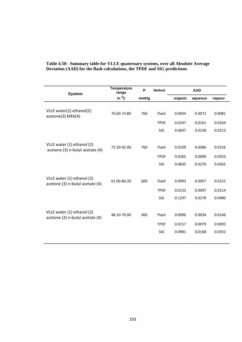
193
Table 4.50: Summary table for VLLE quaternary systems, over all Absolute Average
Deviation (AAD) for the flash calculations, the TPDF and SIG predictions
System
Temperature range
P Method AAD
in 0C mmHg
organic aqueous vapour
VLLE water(1) ethanol(2) acetone(3) MEK(4)
70.60-73.80 760 Flash 0.0044 0.0072 0.0081
TPDF 0.0247 0.0161 0.0164
SIG 0.0697 0.0158 0.0213
VLLE water (1) ethanol (2) acetone (3) n-butyl acetate (4)
72.20-92.00 760 Flash 0.0109 0.0086 0.0156
TPDF 0.0265 0.0099 0.0353
SIG 0.0835 0.0270 0.0362
VLLE water (1) ethanol (2) acetone (3) n-butyl acetate (4)
61.00-80.20 600 Flash 0.0093 0.0057 0.0152
TPDF 0.0133 0.0097 0.0114
SIG 0.1297 0.0278 0.0480
VLLE water (1) ethanol (2) acetone (3) n-butyl acetate (4)
48.10-70.00 360 Flash 0.0096 0.0034 0.0146
TPDF 0.0157 0.0079 0.0093
SIG 0.0981 0.0168 0.0352

194
Table 4.51: Shows UNIQUAC and PRSV EOS interaction parameters for two VLLE
quaternary systems using flash calculations
water(1) ethanol(2) acetone(3) MEK(4)
water (1) ethanol (2) acetone (3) n-butyl acetate (4)
760 mmHg
760 mmHg 600 mmHg 360 mmHg
Parameters
UN
IQU
AC
A12
74.396
-57.65 -18.66 -10.79
A21
-91.49
285.36 499.27 394.34
A23
-636.00
2644.90 -258.50 -193.20
A32
565.33
-278.50 1074.7 639.13
A31
-64.73
583.58 308.19 285.95
A13
770.30
-6.809 175.61 114.08
A24
199.50
-105.90 -145.30 -115.00
A42
421.71
238.41 485.55 379.63
A34
1211.20
-86.82 632.92 701.77
A43
-137.30
123.53 -289.30 -295.20
A14
280.52
626.47 441.94 428.63
A41
526.35
818.91 1176.10 958.92
PR
SV E
OS
k12
0.4779
0.2107 0.1348 0.0765
k23
3E-05
0.2617 1E-05 0.0450
k13
8E-05
0.0577 8E-05 4E-06
K14
1E-07
0.0699 0.1224 0.1069
K34
0.2925
0.0434 0.3132 0.1742
K24
0.0457
0.3303 0.1149 0.0897

195
4.8.1 VLLE water (1) ethanol(2) acetone(3) MEK(4)
Table 4.52: VLLE quaternary system water (1)-ethanol (2)-acetone (3)-MEK (4) at 760 mmHg, experimental Flash, TPDF and SIG predictions
Temperature Experimental Flash calculation TPDF Prediction SIG Prediction
in 0C water ethanol MEK
water ethanol MEK
water ethanol MEK
water ethanol MEK
Organic Phase 73.80 0.44924 0.00890 0.53944
0.45317 0.00833 0.53604
0.44625 0.00413 0.54719
0.39455 0.00329 0.60032
73.40 0.47183 0.01552 0.50844
0.47499 0.01623 0.50449
0.46562 0.00693 0.52401
0.37766 0.00485 0.61492 73.00 0.49451 0.02182 0.47772
0.49756 0.02403 0.47241
0.49450 0.01433 0.48483
0.37743 0.01054 0.60556
72.70 0.52253 0.02768 0.44238
0.52559 0.03175 0.43508
0.51614 0.02538 0.44939
0.38116 0.01822 0.59081 72.50 0.56038 0.03270 0.39862
0.56513 0.03929 0.38671
0.51549 0.03060 0.44388
0.38109 0.02360 0.58317
72.20 0.59520 0.03766 0.35788
0.59577 0.04801 0.34524
0.52037 0.03345 0.43418
0.38288 0.02503 0.57825 72.00 0.63979 0.04010 0.31028
0.63810 0.05583 0.29532
0.52973 0.02930 0.42795
0.38444 0.02148 0.57872
73.20 0.43084 0.00557 0.55942
0.42994 0.00320 0.56393
0.42591 0.00584 0.56436
0.37390 0.00563 0.61589 73.00 0.46087 0.01249 0.51739
0.46156 0.00760 0.52381
0.45580 0.00720 0.52840
0.38130 0.00652 0.60213
72.70 0.49983 0.01911 0.46882
0.50109 0.01223 0.47604
0.47553 0.01360 0.49905
0.38679 0.01203 0.58595 72.40 0.54560 0.02704 0.40864
0.55177 0.01942 0.41210
0.53451 0.01925 0.42804
0.40800 0.02092 0.54799
72.00 0.59385 0.03196 0.35231
0.59965 0.02460 0.35466
0.55422 0.03549 0.38852
0.43449 0.03754 0.50047 71.70 0.69458 0.03347 0.25115
0.70219 0.02922 0.24618
0.55282 0.02959 0.38238
0.42173 0.02862 0.50499
72.80 0.44568 0.00618 0.53796
0.44647 0.00376 0.54216
0.43800 0.00807 0.54127
0.39767 0.01687 0.57053 72.30 0.47550 0.01149 0.49378
0.47917 0.00741 0.49833
0.46997 0.01373 0.49444
0.39561 0.02565 0.55203
72.00 0.50381 0.01668 0.45231
0.51117 0.01130 0.45549
0.50390 0.02007 0.44801
0.41659 0.02331 0.52670 71.80 0.54129 0.02090 0.40440
0.54949 0.01524 0.40665
0.54074 0.02809 0.39958
0.42106 0.03026 0.50893
71.30 0.58878 0.02416 0.34942
0.60040 0.01914 0.34635
0.52817 0.01622 0.41695
0.39888 0.01705 0.53516 71.10 0.66484 0.02534 0.27237
0.67725 0.02243 0.26371
0.57009 0.05000 0.34026
0.44217 0.04809 0.45905
72.40 0.42993 0.00310 0.55902
0.42863 0.00185 0.56382
0.45901 0.00833 0.37197
0.45522 0.00835 0.38535 72.10 0.45538 0.00542 0.51894
0.45682 0.00346 0.52451
0.48471 0.01217 0.35999
0.44398 0.01435 0.38487
71.80 0.47431 0.00774 0.48632
0.47988 0.00526 0.49069
0.48372 0.01315 0.45003
0.40628 0.01517 0.51660 71.30 0.50064 0.01003 0.44822
0.50636 0.00704 0.45413
0.51649 0.02692 0.39597
0.43897 0.03024 0.45998
71.10 0.56792 0.01376 0.36233
0.57658 0.01122 0.36371
0.54331 0.01952 0.38324
0.39963 0.01842 0.51313 70.60 0.60641 0.01560 0.31803
0.61664 0.01355 0.31604
0.55813 0.01680 0.36559
0.47129 0.01312 0.43324
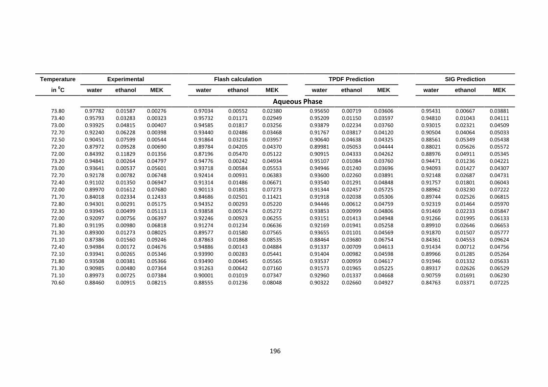
196
Temperature Experimental Flash calculation TPDF Prediction SIG Prediction
in 0C water ethanol MEK
water ethanol MEK
water ethanol MEK
water ethanol MEK
Aqueous Phase 73.80 0.97782 0.01587 0.00276
0.97034 0.00552 0.02380
0.95650 0.00719 0.03606
0.95431 0.00667 0.03881
73.40 0.95793 0.03283 0.00323
0.95732 0.01171 0.02949
0.95209 0.01150 0.03597
0.94810 0.01043 0.04111 73.00 0.93925 0.04815 0.00407
0.94585 0.01817 0.03256
0.93879 0.02234 0.03760
0.93015 0.02321 0.04509
72.70 0.92240 0.06228 0.00398
0.93440 0.02486 0.03468
0.91767 0.03817 0.04120
0.90504 0.04064 0.05033 72.50 0.90451 0.07599 0.00544
0.91864 0.03216 0.03957
0.90640 0.04638 0.04325
0.88561 0.05349 0.05438
72.20 0.87972 0.09528 0.00690
0.89784 0.04205 0.04370
0.89981 0.05053 0.04444
0.88021 0.05626 0.05572 72.00 0.84392 0.11829 0.01356
0.87196 0.05470 0.05122
0.90915 0.04333 0.04262
0.88976 0.04911 0.05345
73.20 0.94841 0.00264 0.04797
0.94776 0.00242 0.04934
0.95107 0.01084 0.03760
0.94471 0.01236 0.04221 73.00 0.93641 0.00537 0.05601
0.93718 0.00584 0.05553
0.94946 0.01240 0.03696
0.94093 0.01427 0.04307
72.70 0.92178 0.00782 0.06748
0.92414 0.00931 0.06383
0.93600 0.02260 0.03891
0.92148 0.02687 0.04731 72.40 0.91102 0.01350 0.06947
0.91314 0.01486 0.06671
0.93540 0.01291 0.04848
0.91757 0.01801 0.06043
72.00 0.89970 0.01612 0.07680
0.90113 0.01851 0.07273
0.91344 0.02457 0.05725
0.88962 0.03230 0.07222 71.70 0.84018 0.02334 0.12433
0.84686 0.02501 0.11421
0.91918 0.02038 0.05306
0.89744 0.02526 0.06815
72.80 0.94301 0.00291 0.05175
0.94352 0.00293 0.05220
0.94446 0.00612 0.04759
0.92319 0.01464 0.05970 72.30 0.93945 0.00499 0.05113
0.93858 0.00574 0.05272
0.93853 0.00999 0.04806
0.91469 0.02233 0.05847
72.00 0.92097 0.00756 0.06397
0.92246 0.00923 0.06255
0.93151 0.01413 0.04948
0.91266 0.01995 0.06133 71.80 0.91195 0.00980 0.06818
0.91274 0.01234 0.06636
0.92169 0.01941 0.05258
0.89910 0.02646 0.06653
71.30 0.89300 0.01273 0.08025
0.89577 0.01580 0.07565
0.93655 0.01101 0.04569
0.91870 0.01507 0.05777 71.10 0.87386 0.01560 0.09246
0.87863 0.01868 0.08535
0.88464 0.03680 0.06754
0.84361 0.04553 0.09624
72.40 0.94984 0.00172 0.04676
0.94886 0.00143 0.04884
0.91337 0.00709 0.04613
0.91434 0.00712 0.04756 72.10 0.93941 0.00265 0.05346
0.93990 0.00283 0.05441
0.91404 0.00982 0.04598
0.89966 0.01285 0.05264
71.80 0.93508 0.00381 0.05366
0.93490 0.00445 0.05565
0.93537 0.00959 0.04617
0.91946 0.01332 0.05633 71.30 0.90985 0.00480 0.07364
0.91263 0.00642 0.07160
0.91573 0.01965 0.05225
0.89317 0.02626 0.06529
71.10 0.89973 0.00725 0.07384
0.90001 0.01019 0.07347
0.92960 0.01337 0.04668
0.90759 0.01691 0.06230 70.60 0.88460 0.00915 0.08215
0.88555 0.01236 0.08048
0.90322 0.02660 0.04927
0.84763 0.03371 0.07225

197
Temperature Experimental Flash calculation TPDF Prediction SIG Prediction
in 0C water ethanol MEK
water ethanol MEK
water ethanol MEK
water ethanol MEK
Vapour Phase 73.80 0.35983 0.00869 0.62717
0.35582 0.01965 0.61700
0.35840 0.00695 0.62945
0.35114 0.00631 0.63859
73.40 0.35687 0.01536 0.61977
0.34835 0.03582 0.60334
0.35663 0.01101 0.62509
0.34375 0.00958 0.64112 73.00 0.35717 0.02206 0.60918
0.34246 0.04989 0.59095
0.34989 0.02050 0.61651
0.33354 0.02000 0.63289
72.70 0.35739 0.02872 0.59878
0.33807 0.06213 0.57956
0.33955 0.03309 0.60947
0.32354 0.03276 0.62382 72.50 0.35884 0.03556 0.58651
0.33677 0.07286 0.56743
0.33407 0.03920 0.60751
0.31657 0.04124 0.61810
72.20 0.35232 0.04181 0.58311
0.32846 0.08450 0.55960
0.33041 0.04151 0.60533
0.31387 0.04289 0.61588 72.00 0.35113 0.04699 0.57628
0.32448 0.09484 0.55387
0.33354 0.03565 0.60546
0.31643 0.03671 0.61606
73.20 0.35332 0.00517 0.63403
0.35154 0.00776 0.63146
0.35104 0.01015 0.63056
0.34012 0.01107 0.63896 73.00 0.35073 0.01224 0.61905
0.34583 0.01667 0.61648
0.35080 0.01128 0.61967
0.33662 0.01215 0.62967
72.70 0.34821 0.01902 0.60437
0.34126 0.02443 0.60404
0.34453 0.01958 0.61143
0.32819 0.02111 0.61880 72.40 0.34799 0.02798 0.58186
0.33619 0.03428 0.58452
0.34335 0.02943 0.60131
0.32914 0.03681 0.60683
72.00 0.33927 0.03461 0.57171
0.32959 0.03963 0.57571
0.33188 0.05053 0.58447
0.32095 0.05941 0.58536 71.70 0.33939 0.04131 0.55419
0.32446 0.04391 0.56986
0.33314 0.04306 0.56987
0.32010 0.04752 0.57702
72.80 0.35393 0.00611 0.61983
0.34865 0.00852 0.61910
0.34567 0.01438 0.62472
0.33123 0.03044 0.62110 72.30 0.34832 0.01145 0.60088
0.34131 0.01479 0.59881
0.34271 0.02294 0.60644
0.32183 0.04574 0.60137
72.00 0.34841 0.01635 0.57896
0.33558 0.02008 0.58101
0.33930 0.03151 0.59088
0.32643 0.03995 0.59323 71.80 0.34185 0.02093 0.56404
0.32949 0.02408 0.56676
0.33455 0.04145 0.57711
0.32228 0.05048 0.57846
71.30 0.34500 0.02514 0.54110
0.32761 0.02712 0.55153
0.34033 0.02524 0.57872
0.32488 0.03075 0.58578 71.10 0.34382 0.02895 0.52413
0.32495 0.02881 0.54141
0.31943 0.06757 0.54731
0.30961 0.07236 0.55157
72.40 0.35013 0.00286 0.63192
0.34940 0.00440 0.62801
0.32477 0.01462 0.43127
0.32505 0.01468 0.44798 72.10 0.34624 0.00539 0.60783
0.34104 0.00717 0.60450
0.32610 0.02037 0.44248
0.31895 0.02497 0.43713
71.80 0.34306 0.00776 0.58584
0.33399 0.00960 0.58299
0.33961 0.02180 0.56695
0.32664 0.02741 0.57029 71.30 0.33662 0.00987 0.56837
0.32563 0.01124 0.56684
0.32940 0.04087 0.54088
0.31854 0.04909 0.53995
71.10 0.32576 0.01398 0.53112
0.31450 0.01359 0.53218
0.33576 0.02968 0.55271
0.31885 0.03276 0.56383 70.60 0.32433 0.01567 0.51380
0.31128 0.01452 0.51911
0.31543 0.01288 0.54136
0.29880 0.01112 0.51396

198
4.8.2 VLLE water (1) ethanol (2) acetone (3) n-butyl acetate (4) at 760 mmHg
Table 4.53: VLLE quaternary system water (1)-ethanol (2)-acetone (3)-n butyl acetate (4) at 760 mmHg, experimental, Flash, TPDF and SIG predictions
Temperature Experimental Flash calculation TPD Prediction SIG Prediction
in 0C water ethanol n-BA
water ethanol n-BA
water ethanol n-BA
water ethanol n-BA
Organic Phase 92.00 0.16469 0.01355 0.80283
0.18537 0.01798 0.77699
0.17048 0.01942 0.79253
0.28224 0.03824 0.66530
89.50 0.19652 0.04823 0.72539
0.20837 0.06273 0.69783
0.19709 0.04550 0.71496
0.32743 0.10326 0.54945 88.50 0.27541 0.10092 0.58033
0.27183 0.12253 0.56213
0.27439 0.09491 0.53622
0.34279 0.13233 0.50236
87.10 0.26244 0.05023 0.65177
0.26542 0.06607 0.63105
0.26657 0.05202 0.63295
0.35909 0.12782 0.47551 84.50 0.28607 0.14653 0.51273
0.28950 0.16284 0.49576
0.29220 0.10553 0.49677
0.45132 0.19620 0.29139
84.20 0.25866 0.09718 0.59530
0.28042 0.11033 0.56247
0.25714 0.05235 0.64195
0.41200 0.16137 0.34618 83.10 0.36187 0.19826 0.37565
0.36285 0.20633 0.36991
0.36034 0.13580 0.36324
0.51344 0.21260 0.20365
82.00 0.26897 0.14371 0.52492
0.28700 0.15427 0.50019
0.26506 0.09804 0.54022
0.48137 0.18180 0.23598 81.00 0.36188 0.19797 0.37027
0.36383 0.20623 0.36307
0.36397 0.13142 0.37027
0.57670 0.19056 0.13786
79.50 0.48265 0.22013 0.23030
0.47523 0.22670 0.23410
0.48161 0.15849 0.19561
0.68267 0.17681 0.05909 90.20 0.20647 0.03665 0.71251
0.21599 0.04915 0.68844
0.20108 0.04743 0.70708
0.29519 0.06323 0.61072
85.40 0.23931 0.07160 0.61384
0.24739 0.08761 0.58861
0.23349 0.07821 0.61261
0.37041 0.12599 0.43201 82.10 0.26103 0.09985 0.54214
0.26686 0.11649 0.51969
0.26572 0.09805 0.53952
0.41683 0.14235 0.31809
81.20 0.29952 0.12445 0.46271
0.31246 0.13513 0.44623
0.29729 0.11602 0.46969
0.44932 0.15815 0.26504 80.10 0.33120 0.14454 0.39734
0.34419 0.15217 0.39004
0.33410 0.12889 0.40546
0.48531 0.16567 0.21419
79.50 0.36552 0.15907 0.34260
0.36667 0.16819 0.34267
0.36752 0.14763 0.33043
0.59412 0.15492 0.13098 79.20 0.40288 0.16801 0.29551
0.40046 0.17664 0.29744
0.39653 0.15845 0.27704
0.59999 0.16177 0.11970
78.00 0.45325 0.17248 0.24309
0.44804 0.18048 0.24963
0.46806 0.16345 0.19760
0.57350 0.16090 0.12443 92.50 0.21427 0.00569 0.76653
0.22358 0.00926 0.75206
0.21743 0.01404 0.75597
0.32658 0.01475 0.64915
88.50 0.21563 0.02924 0.69216
0.22324 0.04011 0.67032
0.21324 0.06459 0.66032
0.30220 0.04750 0.60855 84.10 0.26352 0.05227 0.58771
0.26334 0.06803 0.56739
0.26293 0.10016 0.53721
0.35236 0.09152 0.44775
80.20 0.25845 0.07241 0.53666
0.25847 0.09270 0.49619
0.25647 0.12942 0.47837
0.39547 0.10192 0.33011 79.10 0.28079 0.08924 0.47252
0.28021 0.10310 0.45385
0.28504 0.14634 0.41098
0.43225 0.12067 0.26924
77.00 0.32806 0.11432 0.36544
0.33191 0.12449 0.36269
0.32349 0.14860 0.37137
0.47669 0.12096 0.20282 75.00 0.40023 0.12822 0.27078
0.39967 0.13628 0.27483
0.39913 0.16570 0.25928
0.54486 0.11850 0.13159
73.50 0.48180 0.13083 0.19381
0.47749 0.13833 0.20191
0.48012 0.17397 0.16270
0.62181 0.11108 0.07552 88.10 0.17686 0.01749 0.74106
0.19519 0.02422 0.71253
0.17904 0.04905 0.72579
0.30378 0.03580 0.61477
80.10 0.22959 0.03780 0.56319
0.24239 0.04686 0.54387
0.23465 0.12271 0.51458
0.36016 0.06049 0.38573

199
Temperature Experimental Flash calculation TPD Prediction
SIG Prediction
in 0C water ethanol n-BA
water ethanol n-BA
water ethanol n-BA
water ethanol n-BA
79.30 0.24802 0.04594 0.50126
0.25758 0.05514 0.49118
0.23067 0.12228 0.51972
0.37429 0.06824 0.35377 78.00 0.25618 0.05308 0.45705
0.26829 0.06207 0.45285
0.26373 0.14475 0.43490
0.39386 0.07273 0.31149
77.00 0.29935 0.05937 0.39213
0.30750 0.06817 0.39501
0.29749 0.15691 0.37364
0.41202 0.07717 0.27716 76.20 0.30382 0.06385 0.35987
0.31789 0.07219 0.36615
0.29441 0.14994 0.39561
0.42208 0.07492 0.25746
75.00 0.33468 0.06753 0.31661
0.35226 0.07692 0.33176
0.32259 0.16259 0.33810
0.44133 0.07277 0.22521 74.10 0.39870 0.07429 0.24804
0.41560 0.08379 0.26620
0.40466 0.16346 0.26005
0.47622 0.07964 0.18398
72.20 0.45790 0.07523 0.18248
0.46148 0.08162 0.19266
0.46716 0.17127 0.18285
0.54222 0.07365 0.11712
Aqueous Phase 92.00 0.99098 0.00496 0.00116
0.98981 0.00606 0.00140
0.98972 0.00408 0.00334
0.98419 0.01203 0.00175
89.50 0.97927 0.01469 0.00232
0.96960 0.02313 0.00224
0.97948 0.00989 0.00352
0.95876 0.03508 0.00297 88.50 0.96068 0.03113 0.00189
0.94360 0.04554 0.00317
0.95353 0.02373 0.00460
0.94459 0.04757 0.00391
87.10 0.97672 0.01587 0.00172
0.96935 0.02243 0.00227
0.97977 0.01026 0.00278
0.94476 0.04503 0.00364 84.50 0.94223 0.04559 0.00320
0.91806 0.06662 0.00476
0.94940 0.02637 0.00421
0.88255 0.09086 0.00974
84.20 0.96105 0.02990 0.00216
0.94944 0.03945 0.00311
0.98029 0.01013 0.00255
0.90735 0.06724 0.00663 83.10 0.90928 0.06956 0.00696
0.88085 0.09541 0.00802
0.92228 0.04031 0.00544
0.83515 0.12041 0.01728
82.00 0.94491 0.04358 0.00214
0.92437 0.06025 0.00417
0.95561 0.02331 0.00371
0.85992 0.09388 0.01254 81.00 0.91178 0.06872 0.00493
0.88324 0.09280 0.00721
0.93054 0.03664 0.00451
0.80961 0.12311 0.02078
79.50 0.86849 0.09827 0.01156
0.84153 0.12255 0.01307
0.87713 0.06330 0.00762
0.68413 0.17635 0.05843 90.20 0.98171 0.01181 0.00102
0.97292 0.01750 0.00211
0.97842 0.01043 0.00363
0.97246 0.02063 0.00224
85.40 0.96646 0.02199 0.00176
0.95138 0.03232 0.00284
0.96506 0.01798 0.00373
0.93610 0.04617 0.00413 82.10 0.95164 0.03170 0.00236
0.93185 0.04552 0.00376
0.95563 0.02330 0.00373
0.90082 0.06143 0.00701
81.20 0.93670 0.04109 0.00322
0.91894 0.05403 0.00468
0.94342 0.02973 0.00418
0.87694 0.07571 0.00966 80.10 0.92136 0.05006 0.00426
0.90293 0.06454 0.00590
0.93353 0.03503 0.00443
0.84901 0.08926 0.01351
79.50 0.90691 0.05860 0.00549
0.88259 0.07732 0.00744
0.91021 0.04656 0.00581
0.84077 0.09243 0.01374 79.20 0.89141 0.06725 0.00738
0.86713 0.08632 0.00915
0.88914 0.05661 0.00733
0.81767 0.10500 0.01804
78.00 0.87296 0.07631 0.01052
0.85028 0.09566 0.01193
0.86924 0.06687 0.00824
0.78394 0.11271 0.02546 92.50 0.99498 0.00262 0.00084
0.99313 0.00306 0.00157
0.99273 0.00263 0.00282
0.99281 0.00451 0.00137
88.50 0.98159 0.00955 0.00150
0.97288 0.01418 0.00209
0.97026 0.01485 0.00393
0.97732 0.01477 0.00184 84.10 0.96862 0.01718 0.00147
0.95504 0.02436 0.00266
0.95210 0.02483 0.00423
0.94438 0.03236 0.00340
80.20 0.95565 0.02396 0.00210
0.93200 0.03544 0.00311
0.92405 0.03846 0.00618
0.91140 0.04212 0.00561 79.10 0.94239 0.03007 0.00253
0.92010 0.04146 0.00401
0.90282 0.04846 0.00777
0.88520 0.05610 0.00815
77.00 0.91472 0.04244 0.00432
0.89302 0.05522 0.00614
0.91039 0.04623 0.00591
0.85081 0.06528 0.01215
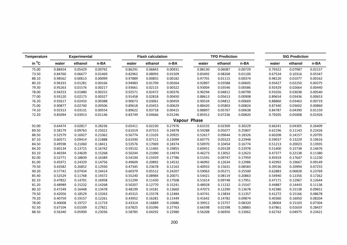
200
Temperature Experimental Flash calculation TPD Prediction
SIG Prediction
in 0C water ethanol n-BA
water ethanol n-BA
water ethanol n-BA
water ethanol n-BA
75.00 0.88454 0.05429 0.00792
0.86291 0.06843 0.00931
0.88130 0.06087 0.00729
0.79322 0.07987 0.02157 73.50 0.84760 0.06677 0.01469
0.82962 0.08093 0.01509
0.83492 0.08268 0.01100
0.67534 0.10316 0.05347
88.10 0.98562 0.00613 0.00099
0.97889 0.00855 0.00182
0.97701 0.01115 0.00374
0.98120 0.01077 0.00162 80.10 0.96333 0.01281 0.00166
0.94983 0.01709 0.00264
0.92897 0.03588 0.00605
0.93427 0.02250 0.00375
79.30 0.95263 0.01576 0.00217
0.93661 0.02115 0.00322
0.93004 0.03546 0.00586
0.92429 0.02664 0.00440 78.00 0.94253 0.01880 0.00252
0.92571 0.02472 0.00376
0.90294 0.04812 0.00799
0.91026 0.03038 0.00540
77.00 0.93120 0.02173 0.00327
0.91458 0.02818 0.00450
0.88613 0.05613 0.00908
0.89654 0.03436 0.00653 76.20 0.92617 0.02433 0.00388
0.90673 0.03061 0.00459
0.90534 0.04812 0.00669
0.88860 0.03463 0.00719
75.00 0.90877 0.02740 0.00506
0.89618 0.03453 0.00629
0.88420 0.05803 0.00824
0.87340 0.03602 0.00860 74.10 0.92313 0.03131 0.00554
0.89622 0.03718 0.00415
0.88897 0.05767 0.00638
0.84787 0.04390 0.01159
72.20 0.85094 0.03913 0.01146
0.83749 0.04666 0.01246
0.85912 0.07236 0.00820
0.79205 0.05008 0.01926
Vapour Phase 92.00 0.64474 0.02817 0.28236
0.65411 0.02230 0.27976
0.63155 0.02309 0.30229
0.66241 0.04305 0.26409
89.50 0.58179 0.09763 0.25022
0.61019 0.07315 0.24978
0.59288 0.05077 0.25807
0.62196 0.11143 0.22426 88.50 0.52579 0.16927 0.21062
0.56774 0.13103 0.20925
0.52617 0.09644 0.18326
0.60208 0.14157 0.20795
87.10 0.60571 0.09414 0.21888
0.61930 0.07111 0.23099
0.60775 0.05523 0.22948
0.59037 0.13229 0.19616 84.50 0.49598 0.21060 0.18411
0.53576 0.17069 0.18374
0.50970 0.10454 0.16774
0.51213 0.20023 0.13935
84.20 0.60134 0.13715 0.16742
0.59132 0.11465 0.19855
0.60451 0.05528 0.22978
0.51400 0.15738 0.14676 83.10 0.46594 0.24639 0.15268
0.50244 0.21090 0.14974
0.46273 0.13052 0.12623
0.47377 0.22138 0.11380
82.00 0.52771 0.18839 0.16389
0.54194 0.15929 0.17786
0.51591 0.09747 0.17959
0.45919 0.17647 0.11230 81.00 0.45971 0.24329 0.14756
0.49609 0.20892 0.14532
0.46992 0.12634 0.12986
0.42992 0.19667 0.09149
79.50 0.43582 0.26852 0.12930
0.47345 0.23678 0.12163
0.40933 0.15631 0.08583
0.39536 0.20994 0.07255 90.20 0.57741 0.07434 0.24414
0.60379 0.05512 0.24207
0.59063 0.05271 0.25500
0.62883 0.06828 0.23769
85.40 0.52529 0.11768 0.19372
0.55240 0.08984 0.20071
0.54421 0.08119 0.20863
0.54940 0.12356 0.17262 82.10 0.47852 0.14701 0.16958
0.51299 0.11430 0.17508
0.51614 0.09748 0.17951
0.47171 0.12967 0.12644
81.20 0.48989 0.15232 0.14268
0.50207 0.12770 0.15241
0.48928 0.11232 0.15547
0.44887 0.14443 0.11136 80.10 0.47249 0.16448 0.13478
0.48199 0.14181 0.13660
0.47073 0.12290 0.13678
0.42380 0.15138 0.09651
79.50 0.42056 0.18529 0.13263
0.45315 0.15578 0.12484
0.43741 0.13834 0.11357
0.41272 0.15166 0.08678 79.20 0.40759 0.19157 0.12261
0.43952 0.16281 0.11449
0.41642 0.14782 0.09874
0.40360 0.16050 0.08204
78.00 0.40008 0.19727 0.11719
0.43314 0.16889 0.10686
0.39912 0.15757 0.08320
0.38004 0.15103 0.07304 92.50 0.67104 0.01509 0.27821
0.67825 0.01096 0.27763
0.66598 0.01598 0.28883
0.67861 0.01659 0.28437
88.50 0.56340 0.05909 0.23036
0.58785 0.04292 0.22980
0.56208 0.06950 0.23062
0.62742 0.04975 0.23421

201
Temperature Experimental Flash calculation TPD Prediction
SIG Prediction
in 0C water ethanol n-BA
water ethanol n-BA
water ethanol n-BA
water ethanol n-BA
84.10 0.50587 0.09008 0.18594
0.53774 0.06594 0.19096
0.51150 0.09998 0.17861
0.52573 0.08440 0.16430 80.20 0.42253 0.11612 0.12972
0.46712 0.08261 0.15280
0.45022 0.12248 0.14832
0.44053 0.08493 0.11584
79.10 0.42230 0.11931 0.14483
0.44741 0.08994 0.14062
0.42472 0.13422 0.12627
0.41499 0.10045 0.09949 77.00 0.38926 0.12880 0.11980
0.41698 0.10458 0.11324
0.42854 0.13588 0.11883
0.37492 0.09790 0.07867
75.00 0.36480 0.13562 0.10219
0.39132 0.11264 0.09326
0.39771 0.15077 0.09174
0.33864 0.09646 0.06053 73.50 0.35416 0.13839 0.09152
0.37690 0.11641 0.08166
0.36756 0.16334 0.07099
0.31261 0.09506 0.04814
88.10 0.57500 0.03641 0.23621
0.59123 0.02676 0.23803
0.57576 0.05525 0.25964
0.63250 0.03700 0.23394 80.10 0.45988 0.05510 0.15534
0.47729 0.04108 0.15948
0.45484 0.11769 0.15894
0.44572 0.04832 0.12447
79.30 0.41673 0.06133 0.14439
0.44139 0.04584 0.13962
0.45391 0.11714 0.15986
0.42869 0.05371 0.11427 78.00 0.39762 0.06556 0.13331
0.41778 0.04975 0.12444
0.42058 0.13237 0.13066
0.40315 0.05566 0.10016
77.00 0.38454 0.06871 0.12201
0.40231 0.05278 0.11049
0.40504 0.14040 0.11343
0.38398 0.05806 0.08960 76.20 0.37545 0.06986 0.11147
0.38739 0.05472 0.09945
0.41928 0.13553 0.12133
0.37006 0.05531 0.08277
75.00 0.39004 0.07534 0.11129
0.38822 0.05861 0.09356
0.39819 0.14395 0.10477
0.34960 0.05246 0.07272 74.10 0.37108 0.07919 0.09873
0.37850 0.06397 0.08243
0.40144 0.14926 0.09332
0.33300 0.05767 0.06356
72.20 0.31902 0.07336 0.07489 0.32944 0.05931 0.06301 0.37558 0.15942 0.07662 0.29908 0.05296 0.04720

202
4.8.3 VLLE water (1) ethanol (2) acetone (3) n-butyl acetate (4) at 600 mmHg
Table 4.54: VLLE quaternary system water (1)-ethanol (2)-acetone (3)-n butyl acetate (4) at 600 mmHg, experimental, Flash, TPDF and SIG predictions
Temperature Experimental Flash calculation TPDF Prediction SIG Prediction
in 0C water ethanol n-BA
water ethanol n-BA
water ethanol n-BA
water ethanol n-BA
Organic Phase 80.20 0.17837 0.05833 0.73417
0.19193 0.04862 0.73006
0.17209 0.03623 0.76152
0.33343 0.07413 0.56804
77.10 0.23142 0.08733 0.64718
0.23997 0.08422 0.63554
0.23284 0.08369 0.64031
0.43962 0.14908 0.36312 74.00 0.27089 0.12788 0.55599
0.28288 0.12365 0.54227
0.28179 0.12642 0.53620
0.59864 0.15482 0.17698
73.00 0.27371 0.17160 0.49911
0.29793 0.15638 0.48725
0.27557 0.12757 0.54069
0.58589 0.15572 0.17312 72.10 0.31928 0.20500 0.41665
0.35044 0.18362 0.40912
0.32393 0.15004 0.46825
0.46626 0.17391 0.23747
71.10 0.48147 0.23427 0.22280
0.49853 0.21905 0.22030
0.48382 0.19367 0.27022
0.68553 0.15553 0.07718 80.00 0.16721 0.03265 0.76384
0.17439 0.03018 0.75077
0.17471 0.03512 0.75124
0.33084 0.07145 0.56665
76.20 0.21375 0.06469 0.65750
0.22253 0.06022 0.64267
0.21236 0.06702 0.63302
0.42322 0.12484 0.37377 74.10 0.23452 0.09786 0.57972
0.25198 0.08633 0.56892
0.23244 0.08313 0.58250
0.46385 0.14022 0.29156
73.10 0.26047 0.12160 0.51455
0.28102 0.10902 0.50197
0.27579 0.10529 0.50777
0.55939 0.14312 0.19941 69.50 0.30336 0.14145 0.44206
0.32220 0.12829 0.43129
0.30991 0.12920 0.44313
0.62977 0.13209 0.11175
68.30 0.39554 0.16886 0.31079
0.41216 0.15607 0.30621
0.40025 0.16083 0.32485
0.69036 0.12696 0.06690 67.20 0.51850 0.16708 0.19930
0.51883 0.16608 0.19696
0.52230 0.17461 0.19226
0.72741 0.12109 0.04212
66.10 0.59206 0.16670 0.13399
0.59492 0.16633 0.13243
0.57238 0.16449 0.14133
0.69581 0.12522 0.04591 79.50 0.14914 0.02279 0.77611
0.15821 0.02026 0.75923
0.14148 0.02190 0.77802
0.30319 0.05361 0.58697
75.40 0.17993 0.04322 0.68137
0.19126 0.03733 0.66297
0.17721 0.04052 0.66130
0.38340 0.09051 0.41052 73.10 0.20151 0.06218 0.60149
0.22070 0.05220 0.58975
0.22361 0.06708 0.56956
0.50655 0.11773 0.25525
70.50 0.22613 0.07936 0.53508
0.24652 0.06667 0.52211
0.24491 0.06701 0.50842
0.55079 0.10758 0.19153 69.10 0.25521 0.09225 0.46927
0.27764 0.07959 0.45956
0.25439 0.07515 0.48596
0.59405 0.10676 0.14076
65.40 0.38340 0.12677 0.27455
0.39983 0.11605 0.27144
0.38875 0.12002 0.28019
0.63150 0.11053 0.07770 64.10 0.45740 0.13289 0.20136
0.46743 0.12572 0.19938
0.43914 0.13098 0.22346
0.61188 0.11212 0.07041
77.00 0.15368 0.01205 0.76725
0.16232 0.00967 0.75380
0.15306 0.01057 0.73954
0.30153 0.03084 0.53848 74.50 0.16678 0.02231 0.68488
0.17970 0.01800 0.66787
0.16936 0.01457 0.65052
0.31655 0.03818 0.47139
71.40 0.18238 0.03139 0.61330
0.19879 0.02505 0.59695
0.18224 0.02042 0.60043
0.34261 0.05181 0.38443 68.30 0.20152 0.04024 0.54472
0.21912 0.03221 0.52845
0.19580 0.03110 0.53656
0.39465 0.07024 0.28086
66.20 0.22289 0.04533 0.49184
0.23979 0.03742 0.47746
0.21114 0.03505 0.49840
0.44138 0.07264 0.21405 64.00 0.27036 0.05757 0.38681
0.28936 0.04813 0.37996
0.24533 0.04130 0.41748
0.52704 0.07121 0.13367
63.00 0.31810 0.06603 0.30710
0.33537 0.05741 0.30371
0.30549 0.06113 0.32055
0.60519 0.07350 0.07988

203
Temperature Experimental Flash calculation TPD Prediction SIG Prediction
in 0C water ethanol n-BA
water ethanol n-BA
water ethanol n-BA
water ethanol n-BA
Organic Phase 62.10 0.37480 0.07027 0.24010
0.38876 0.06374 0.24035
0.35509 0.07939 0.26836
0.60648 0.08095 0.06827
61.00 0.43729 0.07155 0.18604
0.44110 0.06782 0.19119
0.38259 0.07628 0.23515
0.58670 0.07396 0.06581
Aqueous Phase 80.20 0.97880 0.01544 0.00279
0.97436 0.01821 0.00541
0.97464 0.01607 0.00703
0.96199 0.02750 0.00827
77.10 0.96206 0.02979 0.00302
0.95502 0.03322 0.00811
0.94846 0.03689 0.01038
0.91297 0.06353 0.01535 74.00 0.94665 0.04392 0.00192
0.93541 0.04880 0.01003
0.91709 0.05939 0.01597
0.87129 0.08391 0.02121
73.00 0.92919 0.05724 0.00364
0.91678 0.06326 0.01217
0.91602 0.06033 0.01603
0.86171 0.08670 0.02163 72.10 0.90958 0.07034 0.00722
0.89519 0.07898 0.01617
0.89906 0.07210 0.01946
0.79998 0.11318 0.04033
71.10 0.86039 0.10660 0.01171
0.84652 0.11193 0.02319
0.84488 0.10727 0.03241
0.80698 0.11540 0.02829 80.00 0.98308 0.01101 0.00151
0.97802 0.01276 0.00595
0.97433 0.01573 0.00697
0.96240 0.02667 0.00808
76.20 0.96578 0.02258 0.00278
0.95945 0.02597 0.00773
0.94827 0.03270 0.00995
0.92323 0.05231 0.01242 74.10 0.95031 0.03329 0.00268
0.94326 0.03741 0.00917
0.93459 0.04161 0.01173
0.89869 0.06484 0.01525
73.10 0.93781 0.04233 0.00232
0.92906 0.04724 0.01016
0.91638 0.05317 0.01462
0.88367 0.07196 0.01731 69.50 0.92272 0.05200 0.00311
0.91329 0.05696 0.01204
0.89448 0.06725 0.01812
0.83757 0.08396 0.02232
68.30 0.88041 0.07226 0.01409
0.86921 0.08117 0.02016
0.85719 0.08891 0.02596
0.81851 0.09205 0.02206 67.20 0.85699 0.08771 0.01224
0.84908 0.09125 0.02200
0.79998 0.11500 0.03901
0.73616 0.11875 0.03931
66.10 0.80871 0.10856 0.02544
0.80436 0.11196 0.03256
0.78098 0.11739 0.03981
0.70486 0.12310 0.04307 79.50 0.98344 0.00786 0.00269
0.98036 0.00922 0.00584
0.97770 0.01103 0.00669
0.96754 0.02060 0.00701
75.40 0.96965 0.01466 0.00347
0.96575 0.01776 0.00685
0.95809 0.02184 0.00820
0.93807 0.03755 0.00928 73.10 0.95725 0.02137 0.00290
0.95338 0.02498 0.00753
0.93741 0.03553 0.01046
0.91056 0.05265 0.01218
70.50 0.94182 0.02808 0.00451
0.93733 0.03348 0.00907
0.93048 0.03628 0.01012
0.89937 0.05138 0.01196 69.10 0.92687 0.03427 0.00610
0.92179 0.04134 0.01060
0.92244 0.04112 0.01103
0.89299 0.05211 0.01051
65.40 0.87695 0.05639 0.00766
0.87073 0.06372 0.01523
0.85435 0.07147 0.02024
0.79730 0.08012 0.02270 64.10 0.84324 0.06815 0.01348
0.83752 0.07595 0.02018
0.82594 0.08263 0.02500
0.76732 0.08590 0.02287
77.00 0.98683 0.00466 0.00127
0.98509 0.00438 0.00523
0.98207 0.00535 0.00535
0.97031 0.01265 0.00559 74.50 0.97513 0.00805 0.00157
0.97413 0.00890 0.00564
0.97098 0.00825 0.00586
0.96010 0.01641 0.00578
71.40 0.96383 0.01128 0.00217
0.96321 0.01319 0.00616
0.96297 0.01186 0.00601
0.94188 0.02365 0.00647 68.30 0.95209 0.01450 0.00223
0.95106 0.01775 0.00661
0.94559 0.01950 0.00728
0.91389 0.03413 0.00798
66.20 0.94148 0.01744 0.00267
0.94072 0.02127 0.00722
0.93987 0.02176 0.00721
0.89916 0.03605 0.00809 64.00 0.91815 0.02324 0.00371
0.91798 0.02836 0.00859
0.92420 0.02590 0.00772
0.88537 0.03573 0.00759
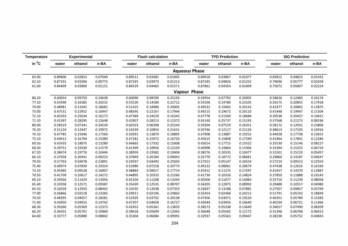
204
Temperature Experimental Flash calculation TPD Prediction SIG Prediction
in 0C water ethanol n-BA
water ethanol n-BA
water ethanol n-BA
water ethanol n-BA
Aqueous Phase 63.00 0.89606 0.02815 0.07040
0.89511 0.03481 0.01005
0.89018 0.03867 0.01077
0.82812 0.04823 0.01432
62.10 0.87191 0.03306 0.00773
0.87245 0.03973 0.01213
0.87245 0.04826 0.01252
0.79696 0.05777 0.01658 61.00 0.84409 0.03800 0.01131
0.84529 0.04465 0.01571
0.87861 0.04354 0.01009
0.75072 0.05897 0.02224
Vapour Phase 80.20 0.60054 0.09750 0.24638
0.60090 0.09590 0.25193
0.59954 0.07792 0.26905
0.58626 0.12483 0.24174
77.10 0.54390 0.16585 0.20232
0.55520 0.14580 0.22712
0.54196 0.14780 0.23105
0.50175 0.20855 0.17918 74.00 0.48981 0.21042 0.18682
0.51425 0.18986 0.20005
0.49532 0.19465 0.20142
0.43377 0.20802 0.12875
73.00 0.47531 0.22952 0.16947
0.48595 0.22167 0.17944
0.49215 0.19672 0.20110
0.41448 0.19947 0.11504 72.10 0.45293 0.25634 0.16173
0.47389 0.24529 0.16343
0.47778 0.21569 0.18684
0.39538 0.20437 0.10431
71.10 0.41397 0.28295 0.12648
0.42907 0.28213 0.12372
0.45140 0.25737 0.15193
0.37568 0.21273 0.08196 80.00 0.58319 0.07341 0.24539
0.60323 0.06398 0.25543
0.59204 0.07519 0.26351
0.58172 0.12031 0.23806
76.20 0.51124 0.12447 0.19972
0.54339 0.10854 0.21631
0.50746 0.12117 0.21126
0.48613 0.17193 0.16916 74.10 0.47785 0.15046 0.17260
0.50391 0.13870 0.18895
0.47908 0.13887 0.19252
0.44028 0.17738 0.13652
73.10 0.44913 0.16794 0.15389
0.47181 0.15972 0.16720
0.45615 0.15808 0.17290
0.41964 0.17841 0.12286 69.50 0.42435 0.18075 0.13280
0.44665 0.17332 0.15008
0.43014 0.17715 0.15522
0.35530 0.15146 0.08227
68.30 0.39751 0.19330 0.11579
0.41399 0.18956 0.12239
0.40998 0.19864 0.13306
0.33394 0.15255 0.06719 67.20 0.38474 0.19776 0.10446
0.38959 0.19582 0.10404
0.38276 0.20535 0.10477
0.31501 0.15219 0.05457
66.10 0.37658 0.20441 0.09223
0.37849 0.20184 0.09043
0.35779 0.18772 0.08681
0.29860 0.14187 0.04647 79.50 0.57763 0.04978 0.23891
0.59597 0.04493 0.25043
0.57552 0.05147 0.26554
0.57224 0.09313 0.22919
75.40 0.49974 0.07839 0.19324
0.52980 0.07218 0.20773
0.49132 0.08061 0.20679
0.47438 0.12616 0.16160 73.10 0.45485 0.09528 0.16907
0.48884 0.09017 0.17714
0.45412 0.11275 0.17597
0.42457 0.14370 0.12887
70.50 0.41709 0.10617 0.14272
0.44895 0.10333 0.15266
0.41730 0.10326 0.14824
0.37850 0.11888 0.10143 69.10 0.39356 0.11429 0.13056
0.42104 0.11208 0.13293
0.40506 0.11077 0.14083
0.35710 0.11239 0.08058
65.40 0.33358 0.12571 0.09387
0.35439 0.12535 0.08707
0.34205 0.12875 0.08992
0.29488 0.10557 0.04980 64.10 0.32018 0.12933 0.08442
0.33535 0.12638 0.07353
0.32837 0.13188 0.07881
0.27507 0.09857 0.03769
77.00 0.56866 0.02518 0.23283
0.59911 0.02196 0.24863
0.55454 0.02468 0.24212
0.51791 0.05192 0.18849 74.50 0.48395 0.04057 0.18281
0.52505 0.03702 0.20138
0.47456 0.03071 0.19220
0.46351 0.05789 0.15283
71.40 0.43050 0.04915 0.14742
0.47207 0.04658 0.16727
0.43644 0.03956 0.16640
0.40194 0.06721 0.11466 68.30 0.39260 0.05369 0.12373
0.42452 0.05361 0.13835
0.38573 0.05338 0.13649
0.34657 0.07490 0.08209
66.20 0.36501 0.05701 0.10960
0.39618 0.05699 0.12042
0.36648 0.05565 0.12172
0.31396 0.06768 0.06423 64.00 0.33777 0.05880 0.08842
0.35304 0.06084 0.09091
0.32937 0.05563 0.09447
0.28238 0.05752 0.04843
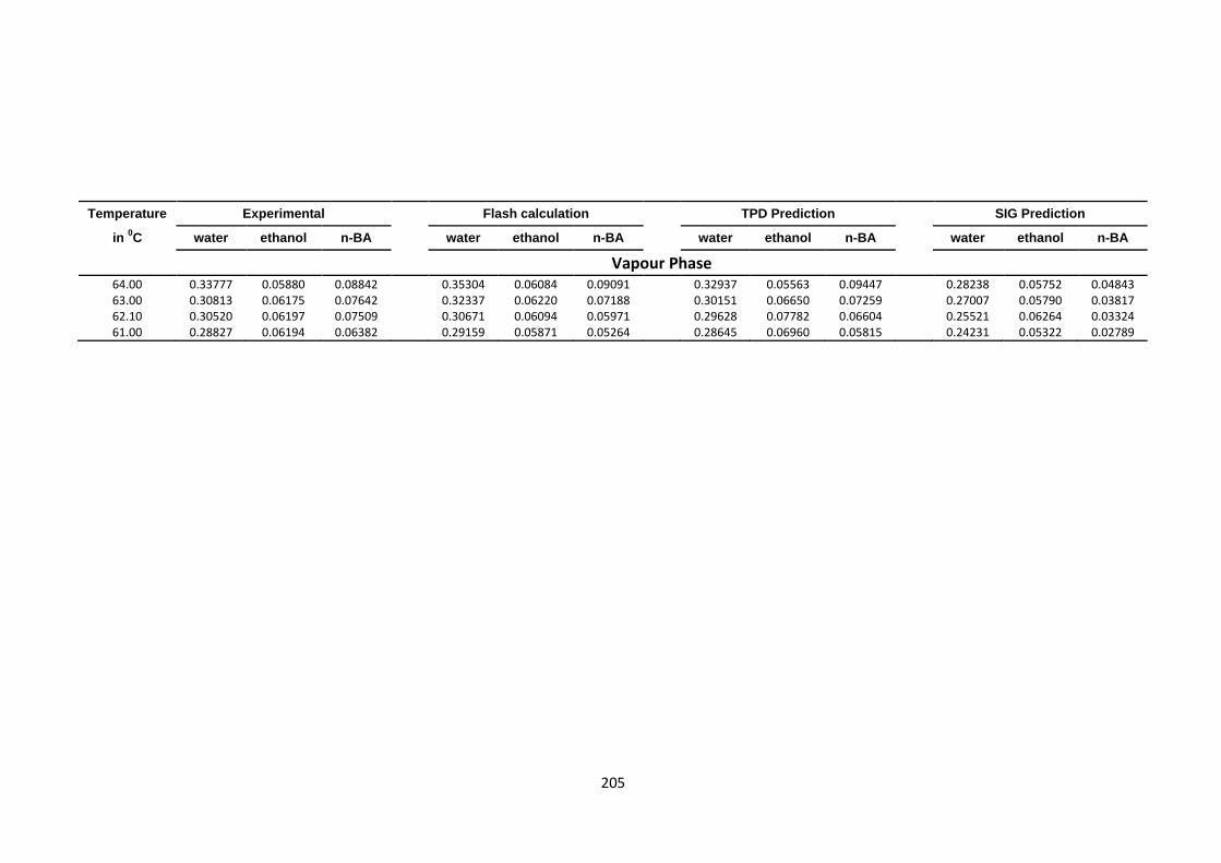
205
Temperature Experimental Flash calculation TPD Prediction SIG Prediction
in 0C water ethanol n-BA
water ethanol n-BA
water ethanol n-BA
water ethanol n-BA
Vapour Phase 64.00 0.33777 0.05880 0.08842
0.35304 0.06084 0.09091
0.32937 0.05563 0.09447
0.28238 0.05752 0.04843
63.00 0.30813 0.06175 0.07642
0.32337 0.06220 0.07188
0.30151 0.06650 0.07259
0.27007 0.05790 0.03817 62.10 0.30520 0.06197 0.07509
0.30671 0.06094 0.05971
0.29628 0.07782 0.06604
0.25521 0.06264 0.03324
61.00 0.28827 0.06194 0.06382 0.29159 0.05871 0.05264 0.28645 0.06960 0.05815 0.24231 0.05322 0.02789

206
4.8.4 VLLE water (1) ethanol (2) acetone (3) n-butyl acetate (4) at 360 mmHg
Table 4.55: VLLE quaternary system water (1)-ethanol (2)-acetone (3)-n butyl acetate (4) at 360 mmHg, experimental, Flash, TPDF and SIG predictions
Temperature Experimental Flash calculation TPDF Prediction SIG Prediction
in 0C water ethanol n-BA
water ethanol n-BA
water ethanol n-BA
water ethanol n-BA
Organic Phase 70.00 0.14377 0.04416 0.78578
0.16081 0.04264 0.76969
0.15432 0.04989 0.76908
0.26840 0.05748 0.66438
66.50 0.17470 0.09238 0.69352
0.19640 0.08341 0.68155
0.18054 0.09398 0.67884
0.37955 0.14123 0.45192 64.10 0.23522 0.13400 0.58052
0.25243 0.12741 0.56922
0.23264 0.12589 0.58409
0.66928 0.14104 0.15749
63.10 0.26314 0.17306 0.50515
0.28474 0.16154 0.49620
0.29744 0.16003 0.48168
0.55704 0.18505 0.20521 62.20 0.31052 0.20001 0.42807
0.33001 0.18834 0.41977
0.36187 0.17162 0.40303
0.57870 0.18355 0.17626
61.10 0.39213 0.22718 0.31596
0.40502 0.21817 0.31001
0.41336 0.18961 0.32940
0.58713 0.18881 0.15132 60.00 0.48229 0.23995 0.21497
0.49257 0.23041 0.21294
0.48088 0.20723 0.24648
0.65684 0.17770 0.09507
72.00 0.15625 0.03162 0.77872
0.17361 0.02902 0.76538
0.15993 0.03083 0.77556
0.25182 0.03450 0.70145 69.00 0.24326 0.05781 0.64329
0.24654 0.05941 0.63601
0.23879 0.06115 0.63734
0.29507 0.05855 0.62549
66.20 0.21561 0.09248 0.60684
0.23786 0.08678 0.59303
0.22410 0.08700 0.60610
0.36024 0.12036 0.47632 62.30 0.29191 0.10955 0.50243
0.29984 0.10832 0.49509
0.28975 0.10331 0.50532
0.41999 0.15240 0.32947
61.10 0.27286 0.14193 0.46923
0.30090 0.12500 0.46771
0.30976 0.10774 0.48596
0.43586 0.15396 0.29455 57.20 0.41687 0.17854 0.26928
0.42815 0.17206 0.26720
0.42297 0.16483 0.28105
0.58862 0.15914 0.12241
56.10 0.54924 0.18004 0.14924
0.55584 0.17536 0.15066
0.52605 0.18029 0.17015
0.67785 0.14687 0.06378 70.10 0.15883 0.02349 0.76789
0.17434 0.01958 0.75674
0.15510 0.02332 0.76391
0.26159 0.02767 0.68968
65.30 0.02474 0.03706 0.65409
0.08733 0.03309 0.79201
0.15233 0.03928 0.70662
0.32531 0.07956 0.51224 62.30 0.19185 0.05792 0.62519
0.20935 0.05351 0.61060
0.19387 0.04793 0.61030
0.34184 0.09209 0.43178
59.20 0.23281 0.07745 0.53325
0.25067 0.07108 0.52425
0.20196 0.06975 0.57159
0.41070 0.12097 0.30242 57.20 0.24561 0.08813 0.49099
0.26573 0.08129 0.48479
0.22431 0.08643 0.51284
0.41070 0.12097 0.30242
54.10 0.36118 0.12596 0.29405
0.37295 0.11939 0.29097
0.30140 0.11608 0.36638
0.74687 0.09160 0.04373 52.10 0.42339 0.13379 0.22356
0.43489 0.12804 0.22379
0.32448 0.12431 0.32993
0.73723 0.08938 0.03439
68.50 0.15421 0.01405 0.76583
0.16819 0.01100 0.75072
0.15313 0.01322 0.74849
0.27049 0.02316 0.65536 64.50 0.15511 0.01949 0.69938
0.17614 0.01775 0.68254
0.14947 0.01679 0.69573
0.29811 0.03803 0.53984
62.40 0.19132 0.02756 0.61040
0.20647 0.02602 0.59670
0.19212 0.02608 0.59873
0.30957 0.05285 0.48151 58.60 0.23197 0.03470 0.53351
0.24071 0.03270 0.52305
0.21319 0.03349 0.53346
0.33799 0.06638 0.37915
55.50 0.21603 0.04187 0.50074
0.23528 0.03843 0.49075
0.20383 0.03466 0.52594
0.36574 0.06827 0.30127 50.60 0.32271 0.06725 0.29422
0.33660 0.06250 0.29330
0.28663 0.05943 0.33876
0.50758 0.07884 0.12919
49.30 0.35732 0.07061 0.24950
0.36940 0.06592 0.25288
0.32668 0.06677 0.28968
0.52459 0.07637 0.10273 48.10 0.45312 0.07368 0.17832
0.44871 0.07135 0.18998
0.42290 0.07733 0.19486
0.54030 0.07172 0.08051
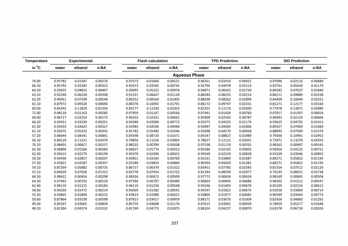
207
Temperature Experimental Flash calculation TPD Prediction SIG Prediction
in 0C water ethanol n-BA
water ethanol n-BA
water ethanol n-BA
water ethanol n-BA
Aqueous Phase 70.00 0.97782 0.01587 0.00276
0.97573 0.01660 0.00521
0.96351 0.02410 0.00921
0.97096 0.02116 0.00689
66.50 0.95793 0.03283 0.00323
0.95473 0.03345 0.00745
0.92795 0.04978 0.01513
0.92761 0.05630 0.01179 64.10 0.93925 0.04815 0.00407
0.93095 0.05222 0.00976
0.90871 0.06425 0.01730
0.89282 0.07637 0.01840
63.10 0.92240 0.06228 0.00398
0.91321 0.06647 0.01120
0.88284 0.08255 0.02214
0.86111 0.09889 0.02228 62.20 0.90451 0.07599 0.00544
0.89252 0.08160 0.01405
0.88500 0.08262 0.01899
0.84409 0.10640 0.02551
61.10 0.87972 0.09528 0.00690
0.86570 0.10092 0.01701
0.86172 0.09747 0.02331
0.81271 0.12177 0.03160 60.00 0.84392 0.11829 0.01356
0.83177 0.12330 0.02303
0.82201 0.12170 0.03300
0.77478 0.13871 0.03989
72.00 0.98118 0.01163 0.00285
0.97959 0.01167 0.00566
0.97441 0.01426 0.00760
0.97917 0.01307 0.00654 69.00 0.96717 0.02254 0.00172
0.96353 0.02331 0.00662
0.95909 0.02565 0.00787
0.96992 0.02124 0.00666
66.20 0.95051 0.03330 0.00251
0.94589 0.03589 0.00772
0.93375 0.04235 0.01174
0.93625 0.04735 0.01013 62.30 0.93433 0.04423 0.00327
0.92983 0.04596 0.00946
0.92897 0.04583 0.01006
0.89327 0.07069 0.01460
61.10 0.92075 0.05332 0.00342
0.91782 0.05400 0.01046
0.93098 0.04570 0.00928
0.88093 0.07509 0.01579 57.20 0.86644 0.08341 0.00841
0.85938 0.08720 0.01671
0.85547 0.08827 0.01989
0.79300 0.10991 0.02952
56.10 0.80129 0.11221 0.02470
0.79856 0.11526 0.03003
0.78627 0.12121 0.03501
0.72971 0.13270 0.04355 70.10 0.98401 0.00817 0.00157
0.98232 0.00789 0.00508
0.97538 0.01119 0.00701
0.98263 0.00997 0.00545
65.30 0.96894 0.01566 0.00260
0.96657 0.01774 0.00552
0.95580 0.02165 0.00892
0.95056 0.03125 0.00751 62.30 0.95615 0.02279 0.00190
0.95379 0.02396 0.00652
0.94569 0.02529 0.00838
0.93109 0.03946 0.00852
59.20 0.94436 0.02857 0.00207
0.93951 0.03183 0.00700
0.92531 0.03890 0.01087
0.89271 0.05822 0.01195 57.20 0.92821 0.03587 0.00357
0.92580 0.03859 0.00860
0.90293 0.05059 0.01381
0.89271 0.05822 0.01195
54.10 0.87269 0.05882 0.00735
0.86727 0.06379 0.01322
0.83451 0.07783 0.02583
0.81554 0.07512 0.02126 52.10 0.84039 0.07026 0.01252
0.83770 0.07454 0.01755
0.81344 0.08599 0.02977
0.76145 0.08421 0.02738
68.50 0.98412 0.00456 0.00298
0.98334 0.00472 0.00509
0.97775 0.00654 0.00624
0.98169 0.00845 0.00504 64.50 0.97462 0.00793 0.00129
0.97390 0.00797 0.00489
0.96603 0.00944 0.00686
0.96503 0.01512 0.00547
62.40 0.96110 0.01215 0.00183
0.96110 0.01234 0.00548
0.95436 0.01403 0.00676
0.95105 0.02216 0.00612 58.60 0.95020 0.01472 0.00219
0.95005 0.01582 0.00591
0.94297 0.01822 0.00675
0.92556 0.03069 0.00714
55.50 0.93845 0.01800 0.00232
0.93823 0.01980 0.00621
0.93805 0.01977 0.00682
0.90349 0.03404 0.00773 50.60 0.87864 0.03238 0.00598
0.87813 0.03617 0.00959
0.88171 0.03670 0.01004
0.82426 0.04860 0.01291
49.30 0.85597 0.03665 0.00839
0.85759 0.04008 0.01176
0.87615 0.03901 0.00939
0.78459 0.05277 0.01648 48.10 0.81394 0.04374 0.01532
0.81769 0.04773 0.01875
0.86324 0.04227 0.00870
0.62578 0.06718 0.05026

208
Temperature Experimental Flash calculation TPD Prediction SIG Prediction
in 0C water ethanol n-BA
water ethanol n-BA
water ethanol n-BA
water ethanol n-BA
Vapour Phase 70.00 0.57381 0.10075 0.25519
0.60451 0.08389 0.25482
0.57000 0.10075 0.27061
0.61812 0.10086 0.25999
66.50 0.51007 0.17071 0.21427
0.55558 0.14220 0.22103
0.50726 0.16376 0.22742
0.53340 0.20302 0.19735 64.10 0.47397 0.21179 0.18697
0.50969 0.19009 0.19090
0.48396 0.19295 0.19738
0.47137 0.21632 0.16701
63.10 0.45365 0.23545 0.17019
0.47984 0.22248 0.17017
0.46553 0.22136 0.17403
0.44342 0.24515 0.13581 62.20 0.43657 0.25173 0.15757
0.45784 0.24441 0.15365
0.46003 0.22580 0.15982
0.42345 0.23984 0.12334
61.10 0.40670 0.27581 0.13108
0.42768 0.26840 0.13111
0.44035 0.23940 0.14324
0.39829 0.23979 0.10633 60.00 0.39970 0.28252 0.12463
0.40974 0.28441 0.11293
0.42171 0.25784 0.12704
0.37527 0.23798 0.09186
72.00 0.63206 0.06312 0.22922
0.62121 0.05721 0.25476
0.58870 0.06369 0.27481
0.63077 0.06429 0.27854 69.00 0.53645 0.11591 0.20434
0.56113 0.09961 0.21760
0.54655 0.10314 0.21906
0.60618 0.09931 0.24862
66.20 0.49677 0.14022 0.18376
0.51131 0.13420 0.18433
0.48889 0.13904 0.19694
0.52921 0.17429 0.19555 62.30 0.46766 0.15864 0.15337
0.47543 0.15136 0.16425
0.46582 0.14599 0.16692
0.43369 0.18795 0.13406
61.10 0.49906 0.15067 0.12879
0.45581 0.16588 0.14763
0.46986 0.14963 0.16551
0.40829 0.18147 0.11887 57.20 0.35655 0.19455 0.11070
0.37718 0.19182 0.10061
0.37691 0.18499 0.10674
0.33114 0.17276 0.07342
56.10 0.34069 0.19832 0.09669
0.35335 0.19597 0.08237
0.34744 0.19656 0.08492
0.31063 0.17308 0.06068 70.10 0.59055 0.04337 0.23773
0.60878 0.03884 0.24899
0.56460 0.04839 0.26154
0.63589 0.05093 0.26794
65.30 0.48134 0.08025 0.19956
0.50729 0.07310 0.21664
0.48399 0.07522 0.21966
0.51335 0.11714 0.18631 62.30 0.43240 0.09447 0.17255
0.48150 0.08616 0.17491
0.44064 0.07861 0.17373
0.44282 0.12022 0.14285
59.20 0.41113 0.10433 0.14949
0.43999 0.10097 0.14583
0.41015 0.10586 0.15704
0.37608 0.13429 0.10307 57.20 0.38536 0.11291 0.13428
0.41709 0.10894 0.13165
0.37988 0.11871 0.13559
0.37608 0.13429 0.10307
54.10 0.31470 0.12271 0.09451
0.33002 0.12188 0.08059
0.32636 0.12715 0.09375
0.28835 0.10623 0.06068 52.10 0.30232 0.12406 0.08332
0.31500 0.12284 0.06881
0.31335 0.12853 0.08486
0.25855 0.09526 0.04357
68.50 0.54798 0.02379 0.24212
0.59028 0.02204 0.24088
0.54096 0.02743 0.24644
0.60542 0.04120 0.24410 64.50 0.46229 0.03737 0.19266
0.51883 0.03272 0.19582
0.46482 0.03267 0.20602
0.50066 0.05784 0.17834
62.40 0.41177 0.04525 0.15976
0.45734 0.04227 0.15962
0.42399 0.04295 0.16153
0.45077 0.07316 0.14831 58.60 0.37650 0.04956 0.13592
0.41727 0.04727 0.13459
0.38232 0.04906 0.13180
0.37234 0.07711 0.10345
55.50 0.35651 0.05284 0.12122
0.37988 0.05234 0.11388
0.35952 0.04964 0.12290
0.31792 0.06815 0.07472 50.60 0.27712 0.05964 0.07685
0.28876 0.05938 0.06117
0.27647 0.05926 0.06674
0.24352 0.05933 0.03901
49.30 0.26536 0.05800 0.06587
0.27626 0.05831 0.05394
0.26744 0.06077 0.05827
0.22638 0.05437 0.03145 48.10 0.25959 0.05882 0.06056
0.26263 0.05760 0.04951
0.25255 0.06082 0.04533
0.21147 0.04865 0.02529

209
4.9 Discussion
The correlation and predictions for two quaternary VLLE systems of: water (1)
ethanol (2) acetone (3) MEK (4) at pressure of 760 mmHg and water (1) ethanol
(2) acetone (3) n-butyl acetate (4) system at pressures of 360, 600 and 760
mmHg have been carried out using the PRSV+WSMR model. The Rachford-
Rice method is used in flash calculations and the interaction parameters for
PRSV EOS and the UNIQUAC energy parameters obtained were used in the
TPDF and SIG prediction methods. A quaternary system requires 18
parameters: 12 energy parameters for the UNIQUAC model and 6 interaction
parameters for PRSV EOS. Table (4.51) shows these parameters for both VLLE
systems of interest.
From the results obtained for binary and ternary LLE, VLE and VLLE
calculations it was found that the PRSV+WSMR combination is capable of
correlating the non-ideal polar heterogeneous mixtures and thus it would appear
that this can be extended to quaternary systems.
The results obtained for the quaternary systems using: Flash, TPDF and SIG
methods indicate the capability of these methods to correlate and hence predict
the phase behaviour for quaternary multiphase systems at low and moderate
pressures and moderate temperatures. The summary of the results in table
(4.50) shows the Absolute Average Deviations (AAD) from experimental values
for the Flash, TPDF and SIG in each phase. The TPI method has not been
tested on the quaternary systems and the reasons are discussed in the
previous section (4.7). Overall the AAD TPDF results for the quaternary system
with the constituent binary of MEK-water were less accurate than the system
with the constituent binary of n-butyl acetate-water. Table (4.52) shows the
results for the VLLE system water (1) ethanol (2) acetone (3) MEK (4) at 760
mmHg. Figure (4.41) gives a graphical representation of the composition of
water and MEK components for TPDF predicted values versus the experimental
values in three phases. An observation of the summary table (4.50) shows that
the TPDF AAD is lower than the SIG. Observation of table (4.50) immediately
indicates that the TPDF method gives consistently lower values than the SIG
method. As shown in sections (3.11 and 4.6.3) the SIG method can be used to
generate initial values for the TPI method and it is also capable of extension to
210
quaternary systems. The SIG method depends on an initial generation of phase
compositions using activity coefficients which are used to generate fugacity
coefficients which can then be used to calculate initial (K) values. These are
used to calculate relative volatilities which are employed in a flash calculation.
The SIG results contrast with the TPDF method which is essentially minimising
a function directly related to the Gibbs energy surface. Such an approach
emphasises that the TPDF method is reliable and efficient in predicting
quaternary data.
Observing the data for the quaternary systems it is noticeable that at all
temperatures and pressures there is a consistently high concentration of water
in the organic phase even at low concentrations of other organic components.
Although the TPDF method can produce acceptably low values of AAD for all
phases it is noticeable that the AAD values for the organic phase are
consistently higher than for the aqueous phase. This high water content of the
organic phase is present for all the measured data and is apparently higher than
the theoretical predictions. This is expected as the SIG method is based on the
calculation of the relative volatility of component 𝑖 in the mixture. The behaviour
of constituent heterogeneous binaries azeotrope of (water-MEK) and (water-n
butyl acetate) have the influence on pseudo ternary systems behaviour. The
overall AAD for this system is 0.0065 in Flash calculation, the value in TPDF
prediction is 0.019 and 0.035 for the SIG.
The results for the VLLE correlation and predictions using TPDF and SIG for the
system of water (1) ethanol (2) acetone (3) n-butyl acetate (4) at pressures of
760, 600, 360 mmHg can be found in tables (4.53, 4.54 and 4.55) respectively.
The graphical illustrations for water and n-butyl acetate predictions against
measured data are shown in figures (4.42, 4.43 and 4.44) for this system at
pressure of 760, 600, 360 mmHg respectively.

211
Figure 4.41: VLLE quaternary system water (1)-ethanol (2)-acetone (3)-MEK (4) at 760
mmHg, TPDF prediction versus experimental of water and MEK in the organic, aqueous
and vapour phases
0.0
0.1
0.2
0.3
0.4
0.5
0.6
0.7
0.8
0.9
1.0
0.0 0.2 0.4 0.6 0.8 1.0
organicAqueousVapour
water mole fraction experimental
wat
er m
ole
fra
ctio
n T
PD
F
0.0
0.1
0.2
0.3
0.4
0.5
0.6
0.7
0.8
0.9
1.0
0.0 0.2 0.4 0.6 0.8 1.0
organicAqueousVapour
MEK mole fraction experimental
MEK
mo
le f
ract
ion
TP
DF

212
Figure 4.42: VLLE quaternary system water(1)-ethanol(2)-acetone(3)-n-butyl
acetate(4) at 760 mmHg , TPDF prediction versus experimental of water and n-butyl
acetate in the organic ,aqueous and vapour phases
0.0
0.1
0.2
0.3
0.4
0.5
0.6
0.7
0.8
0.9
1.0
0.0 0.2 0.4 0.6 0.8 1.0
organic
Aqueous
Vapour
water mole fraction experimental
wat
er m
ole
fra
ctio
n T
PD
F
0.0
0.1
0.2
0.3
0.4
0.5
0.6
0.7
0.8
0.9
1.0
0.0 0.2 0.4 0.6 0.8 1.0
organic
Aqueous
Vapour
n-Butyl Acetate mole fraction experimental
n-B
uty
l Ace
tate
mo
le f
ract
ion
TP
DF
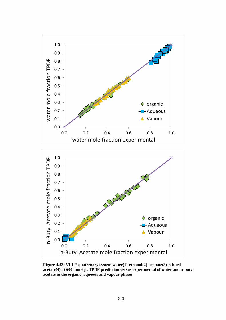
213
Figure 4.43: VLLE quaternary system water(1)-ethanol(2)-acetone(3)-n-butyl
acetate(4) at 600 mmHg , TPDF prediction versus experimental of water and n-butyl
acetate in the organic ,aqueous and vapour phases
0.0
0.1
0.2
0.3
0.4
0.5
0.6
0.7
0.8
0.9
1.0
0.0 0.2 0.4 0.6 0.8 1.0
organic
Aqueous
Vapour
water mole fraction experimental
wat
er m
ole
fra
ctio
n T
PD
F
0.0
0.1
0.2
0.3
0.4
0.5
0.6
0.7
0.8
0.9
1.0
0.0 0.2 0.4 0.6 0.8 1.0
organic
Aqueous
Vapour
n-Butyl Acetate mole fraction experimental
n-B
uty
l Ace
tate
mo
le f
ract
ion
TP
DF
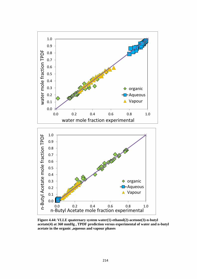
214
Figure 4.44: VLLE quaternary system water(1)-ethanol(2)-acetone(3)-n-butyl
acetate(4) at 360 mmHg , TPDF prediction versus experimental of water and n-butyl
acetate in the organic ,aqueous and vapour phases
0.0
0.1
0.2
0.3
0.4
0.5
0.6
0.7
0.8
0.9
1.0
0.0 0.2 0.4 0.6 0.8 1.0
organic
Aqueous
Vapour
water mole fraction experimental
wat
er m
ole
fra
ctio
n T
PD
F
0.0
0.1
0.2
0.3
0.4
0.5
0.6
0.7
0.8
0.9
1.0
0.0 0.2 0.4 0.6 0.8 1.0
organicAqueousVapour
n-Butyl Acetate mole fraction experimental n-B
uty
l Ace
tate
mo
le f
ract
ion
TP
DF

215
5. Conclusions and Future work
This work has investigated the possibility of thermodynamic modelling of
phase equilibria for a range of homogenous and heterogeneous systems
particularly for VLLE binary, ternary and quaternary systems by utilising the
PRSV EOS combined with WSMR. This modelling package combining PRSV
with WSMR was initially tested on the correlation of VLE binary systems
under isothermal and isobaric conditions. These mixtures have a range of
polar components from moderately polar (MEK, n-butyl acetate) to highly
polar (ethanol, propanol) components. The results obtained show that the
selected modelling package can successfully and adequately represent the
thermodynamic behaviour of fugacity in both liquid and vapour phases.
The Area Method and the TPI method were applied to predict the phase
equilibrium of two LLE and four binary VLLE systems and subsequently the
TPI method was extended to predict binary VLLE. This was achieved by
modifying a 2-point search and a direct 3-point search. Due to the sensitivity
of the TPI to initial conditions, this work developed and successfully applied a
new scheme of fixed initial values which depend on phase change (Cusps)
compositions. The AM method is computationally slower than the TPI due to
the integration part of the Gibbs energy curve, for this reason the AM was
only applied to LLE binary systems.
In the prediction of VLLE for ternary systems, it was outlined in the literature
survey (2.6) that the majority of the optimisation methods require a good
initial estimate to improve their reliability and efficiency. A significant
achievement of this work was in suggesting a Systematic Initial Generator
(SIG) to obtain initial values as close as possible to the real solution. This
had a positive effect in decreasing the fitting error of the TPI results. This
work has, through modelling, identified a problem (i.e. sensitivity to the
starting value) when applying the TPI on VLLE ternary systems. This
research has tested another method of Gibbs free minimisation called the
TPDF method which was used to predict using the VLLE ternary systems of
Younis et al. (2007). This work concludes that the TPDF method is less
sensitive to the initial values, computationally faster than the TPI method and
216
can also be extended to multicomponent multiphase systems with fewer
complications.
Another achievement of this work has been in testing the TPI, TPDF and SIG
methods as a phase predictor on ternary VLLE systems. The TPDF and SIG
method were capable of recognising the 2 and 3-Phase regions successfully,
however the TPI method failed to identify the 2-phase region. This work has
made a useful and effective thermodynamic tool available for engineers
working in design and optimisation of chemical process operation. The
parameters obtained for the VLLE ternary systems can be available for
designers in the field of separation processes within the chemical industry.
Finally this work has applied the thermodynamic package PRSV+WSMR
successfully to two quaternary systems measured by Younis et al. (2007)
using flash correlation whilst obtaining reasonable prediction results for the
TPDF and SIG methods. All multicomponent systems investigated in this
work display highly non-ideal behaviour in that the liquid phase is
heterogeneous for a range of compositions. To use an Equation of State for
such systems requires applicable and effective mixing rules. It is extremely
rare to find examples of an EOS approach to correlating and predicting
highly polar, non-ideal, organic-aqueous systems of low pressures. This work
has demonstrated that the Wong-Sandler mixing rules (WSMR) combined
with the Peng Robinson Styrjek Vera (PRSV) Equation of State, gives an
approach which is fully capable of representing such systems and this
method allows both liquid and vapour phases to be represented by the same
equations.
The Nelder-Mead optimisation simplex was used in correlation and prediction
methods. The main advantage of this optimisation is that it can be used
directly to an objective function without the need for derivative of the function.
It is well known in the thermodynamic field that the Gibbs free minimisation
has non-convex and non-linear properties which indicate that this type of
function has several local minima. It is recommended that further research
be undertaken to investigate the effect and effectiveness of different
optimisation methods on the overall results for VLLE ternary and quaternary

217
systems particularly the modified Nelder-Mead mentioned previously in the
theory chapter (section 3.2).
To evaluate the success of modelling the organic/aqueous heterogeneous
mixtures with partial miscibility using PRSV+WSMR at atmospheric pressure,
this work has used absolute average deviation values as defined at
appropriate points in the text. The results relating to binary, ternary and
quaternary VLLE systems can be found in tables 4.16, 4.20 and 4.50
respectively. In order to illustrate the level of success of the correlations and
the predictions of the TPI and TPDF methods, the AAD results for a complex
mixture of binary VLLE water - n-butyl acetate at 91.050C and 760 mmHg are
0.001 and 0.0005 for correlation and TPI prediction respectively. In the VLLE
ternary system of water-acetone-n butyl acetate for a temperature range
(66.1-86.1)0C and pressure 760 mmHg the overall AAD value related to
composition for the correlation results using flash is 0.004, the value is 0.004
for the TPDF method and 0.03 for the TPI prediction method. For VLLE
quaternary system of water-ethanol-acetone-n-butyl acetate for a
temperature range (48.1-70)0C and pressure 360 mmHg the overall AAD for
the correlation is 0.009 and 0.011 for the TPDF method. The AAD is used by
other researchers as a measure of success in terms of the correlations and
predictions. The smaller the AAD value the more successful the results. The
figures obtained in conjunction with an inspection of the data indicate the
claimed success and superiority of the TPDF method over the TPI method.
To further develop this work the TPDF should be applied to the prediction of
VLLE ternary and quaternary systems calculation using the UNIFAC and
NRTL equation in place of UNIQUAC to calculate the excess Gibbs energy
of mixing in the PRSV+WSMR.
This work has exclusively used Wong Sandler Mixing Rules (WSMR)
because an examination of the literature indicated that it is the most effective
mixing rule when polar molecules are present in a mixture. For future work it
is important that other mixing rules are investigated in order to find out the
effect on the overall correlation and prediction results.

218
This work has used the data available from Younis et al (2007) and the data
available from DECHEMA. It is noticeable that there is a shortage of data for
heterogeneous polar systems at relatively low pressure and yet these
systems are of both theoretical and practical importance. It would be useful
to produce more experimental data on such systems to allow theoretical
models to be tested against a wide range of data.
219
6. References
Abrams, D.S., Prausnitz, J.M., (1975) 'Statistical thermodynamics of liquid
mixture. A new expression for the excess Gibbs energy of partly or
completely miscible systems'. AIChE Journal, 21(1), pp. 116-128.
Alvarez, V. H., R. Larico, Y. Ianos, M. Aznar (2008) 'Parameter estimation for
VLE calculation by global minimization: the genetic algorithm', Braz. Journal
of Chem. Eng.,25, pp. 409-418.
Ammar, M.N., Renon,H.(1987) ' The isothermal flash problems: new
methods for phase split calculations', AIChE Journal, 33, pp. 926-939.
Babu, K. S., M.V.P. Kumar, N. Kaistha (2009) 'Controllable optimized
designs of an ideal reactive distillation system using genetic algorithm',
Chem. Eng. Sci., 64, pp. 4929-4942.
Bollas, G.M., Barton, P.I., Mitsos, A. (2009) 'Bilevel optimization formulation
for parameter estimation in vapor-liquid(-liquid) phase equilibrium problems',
Chemical Engineering Science, 64, pp. 1768-1783.
Bonilla-Petriciolet , A. (2007) ' Reliable Initialization Strategy for the Equal
Area Rule in Flash Calculations of Ternary Systems', Afinidad , 64 (530),pp.
529-534.
Bonilla-Petriciolet, A., Bravo-Sanchez, U.I. , Castillo-Borja,F., Zapiain-
Salinas, J.G., Soto Bernal,J.J. (2007) 'The performance of Simulated
Annealing in parameter estimation for vapor-liquid equilibrium modeling',
Braz. J. Chem. Eng., 24, pp. 151-162.
Bonilla-Petriciolet, A., Rangaiah, G.P., Segovia-Hernández, J.G. (2010)
'Evaluation of stochastic global optimization methods for modeling vapor-
liquid equilibrium data', Fluid Phase Equilibria. 287, pp. 111-125.
Burgos-Solorzano, Gabriela I., Brennecke, Joan F. & Stadtherr, Mark A.
(2004) 'Validated computing approach for high-pressure chemical and
multiphase equilibrium', Fluid Phase Equilibria 219, pp.245–255.
220
Carrier, B., Rogalski, M., Peneloux, A. (1988) 'Correlation and prediction of
physical properties of hydrocarbons with the modified Peng-Robinson
equation of state: 1. Low and medium vapor pressure', Ind. Eng. Chem. Res.
27, pp. 1714-1721.
Coutsikos,P.,Kalospiros,N.S., Tassios,D.P.(1995) 'Capabilities and
limitations of the Wong-Sandler mixing rules', Fluid Phase Equilibria, 108, pp.
59-78.
Desai, G.H.I, 1986. Measurement and correlation of vapour-liquid equilibrium
of heterogeneous system. Ph.D Thesis. Chemical Engineering Department ,
Teesside Polytechnic.
Eubank P.T., Hall K.R. (1995) ' Equal area rule and algorithm for determining
phase compositions', AIChE Journal, 41(4), pp. 924-927.
Eubank, P.T. and Barrufet, M.A. (1988) 'A simple algorithm for calculations of
phase separation', Chemical Engineering Education, 22, pp. 36.
Eubank, P.T. and Hall, K.R. (1995) 'An area rule and algorithm for
determining phase compositions', AIChE Journal, 41, pp. 924-927.
Eubank, P.T., Elhassan, A.E., Barrufet M.A. and Whiting, W.B. (1992) ' Area
method for prediction of fluid phase equilibria', Ind. Eng. Chem. Res., 31, pp.
942-949.
Gao, F., Han, L. (2012) 'Implementing the Nelder-Mead Simplex Algorithm
with Adaptive Parameters', Computational Optimization and Applications,
51(1), pp. 259-277
Garcia-Flores, B., ‘Águila-Hernández, J., García-Sánchez, F., Aquino-Olivos,
M.(2013)’(liquid–liquid) equilibria for ternary and quaternary systems of
representative compounds of gasoline + methanol at 293.15 K: Experimental
data and correlation’ , Fluid Phase Equilibria,348, pp. 60 – 69.
Gecegormez, H., Demirel, Y., (2005) 'Phase stability analysis using interval
Newton method with NRTL model', Fluid Phase Equilibria.237, pp. 48–58.
221
Geem, Z.W.; Kim, J.H. & Loganathan, G.V. (2001) ' A new heuristic
optimization algorithm: harmony search', Simulation, 76(2), pp. 60-68.
Ghosh, P., Taraphdar, T. (1998) 'Prediction of vapor-liquid equilibria of binary
systems using PRSV equation of state and Wong Sandler mixing rules',
Chemical Engineering Journal, 70, pp.15-24.
Gmehling, J., Onken, U. (1977) Vapor-Liquid Equilibrium Data Collection 1.
DECHEMA, Frankfurt.
Gmehling, J., Onken,U. and Arlt, W. (1981) Vapor-liquid equilibrium data
collection. aqueous-organic systems (Supplement 1). Frankfurt/ Main,
DECHEMA Chemistry Data Series Vol. 1a, DECHEMA.
Gmehling, J., Onken,U. and Arlt, W. (1982) Vapor-liquid equilibrium data
collection. Alcohols (Supplement 1). Frankfurt/Main DECHEMA Chemistry
Data Series Vol. 2, DECHEMA.
Gmehling, J., Onken,U. and Arlt, W. (1991) Vapor-liquid equilibrium data
collection. Aqueous-Organic systems (Supplement 1). Frankfurt/Main
DECHEMA Chemistry Data Series Vol I. Part 1 , DECHEMA.
Green, K.A., Zhou, S. and Luks, K.D. (1993) 'The fractal response of robust
solution techniques to the stationary point problem', Fluid Phase Equilibria,
84, pp. 49-78.
Haugen, Kjetil B. and Firoozabadi, A. (2011) 'Efficient and Robust Three-
Phase Split computations', AIChE Journal ,57(9),pp. 2555-2565.
Henderson, N., de Oliveira, J.R., Amaral Souto, H.P. & Pitanga, R. (2001) '
Modeling and analysis of the isothermal flash problem and its calculation with
the simulated annealing algorithm', Industrial Engineering Chemistry
Research, 40(25), pp. 6028-6038.
Hendriks, E.M., van Bergen, A.R.D. (1992) 'Application of a reduction
method to phase equilibria calculations', Fluid Phase Equilibria. 74, pp. 17–
34.
222
Hinojosa-Gomez, H., Barragan-Aroche J. Fernando , Bazua-Rueda Enrique
R. (2010) ' A modification to the Peng–Robinson-fitted equation of state for
pure substances', Fluid Phase Equilibria, 298, pp.12-23
Hodges, D., Pritchard, D.W., Anwar, M.M. (1997) 'Calculating binary and
ternary multiphase Equilibria: extensions of the integral area method', Fluid
Phase Equilibria, 130, pp. 101-116.
Hodges, D., Pritchard, D.W., Anwar, M.M. (1998) 'Calculating binary and
ternary multiphase Equilibria: the tangent plane intersection method', Fluid
Phase Equilibria, 152, pp. 187–208.
Hsieha, Cheng-Ting, Ming-JerLeeb, Ho-mu Linb, Ju-Chun Chengb, Wan-Yun
Ji (2011) 'Multiphase equilibria for mixtures containing water, isopropanol,
propionic acid, and isopropyl propionate', Fluid Phase Equilibria, 305 , pp.
53–61.
Huron, M. and J. Vidal(1979) 'New Mixing Rules in Simple Equation of State
for representing Vapor-Liquid Equilibrium of strongly non-ideal mixtures',
Fluid Phase Equilibria, 3, pp. 255-271.
Iglesias-Silva , Gustavo A. ,Bonilla-Petriciolet,A., Eubank, Philip T., Holste,
James C. , Kenneth R. H. (2003) 'An algebraic method that includes Gibbs
minimization for performing phase equilibrium calculations for any number of
components or phases ',Fluid Phase Equilibria, 210, pp. 229–245.
Justo-García, D., García-Sánchez, F., Díaz-Ramírez, N.,Díaz-Herrera,E.
(2010)‘ Modeling of three-phase vapor–liquid–liquid equilibria for a natural-
gas system rich in nitrogen with the SRK and PC-SAFT EoS’, Fluid Phase
Equilibria,298, pp. 92 – 96.
Kangas, J.,Malinen, I.,Tanskanen,J.(2011) 'Modified bounded homotopies in
the solving of phase stability problems for liquid–liquid phase-splitting
calculations.', Ind.Eng.Chem.Res, 50, pp.7003–7018.
Khodakarami, B., Modarress, H. and Lotfollahi,M. N.(2005) 'Study of the
High-Pressure Vapor-Liquid Equilibria for Strongly Non-Ideal Binary and

223
Ternary Mixtures', Canadian Journal of Chemical Engineering, 83(2), pp.
354-357.
Kirkpatrick, S., C. Gelatt, M. Vecci (1983) 'Optimization by Simulated
Annealing', Science, 220, pp. 671-680.
Kontogeorgis, Georgios M. and Rafiqul G. (2004) Computer Aided Property
Estimation for Process and Product Design. Computers Aided Chemical
Engineering, Volume 19, London, ELSEVIER.
Kosuge ,H., Iwakabe, K.(2005)‘Estimation of isobaric vapor–liquid–liquid
equilibria for partially miscible mixture of ternary system’ , Fluid Phase
Equilibria,233, pp. 47 – 55.
Lee, Ming-Tsung, Lin, Shiang-Tai (2007) 'Prediction of mixture vapor-liquid
equilibrium from the combined use of Peng-Robinson equation of state and
COSMO-SAC activity coefficient model through Wong-Sandler mixing rule',
Fluid Phase Equilibria , 254(1-2), pp. 28-34.
Lee, Y.P.; Rangaiah, G.P. & Luus, R. (1999) 'Phase and chemical
equilibrium calculations by direct search optimization', Computers and
Chemical Engineering, 23(9), pp. 1183-1191.
Leibovici, Claude F. (2006), 'Initialization of vapor–liquid equilibrium
constants for non-hydrocarbon liquid phases', Fluid Phase Equilibria, 248,
pp. 217–218.
Li, J., Chen,C., Wang, J.(2000)’Vapor–liquid equilibrium data and their
correlation for binary systems consisting of ethanol, 2-propanol, 1,2-
ethanediol and methyl benzoate’, Fluid Phase Equilibria,169, pp. 75 – 84.
Li, Z. and Firoozabadi, A. (2012) ' General strategy for stability testing and
phase split calculation in two and three phases', SPE Journal, 17 (4), pp.
1096-1107.
Li, Z., Firoozabadi, A. (2012) 'initialization of phase fractions in Rachford-
Rice equations for robust efficient three-phase split calculation', Fluid Phase
Equilibria, 332, pp. 21-27.
224
Lin, B., Miller, D.C. (2004) 'Tabu search algorithm for chemical process
optimization', Comp. Chem. Eng., 28, pp. 2287-2306.
Lin, Ming-Hua ,Tsai, Jung-Fa ,Yu, Chian-Son (2012) 'A Review of
Deterministic Optimization Methods in Engineering and management',
Mathematical Problems in Engineering , 2012, pp. 15.
Lin, Y., & Stadtherr, M. A. (2004) 'Advances in interval methods for
deterministic global optimization in chemical engineering', Journal of Global
Optimization, 29,pp. 281–296.
Liu, Y., Kusano,R., Iwai,Y.(2012) 'Correlation of Vapor-Liquid Equilibria of
Supercritical Methanol+ Glycerol System', Journal of Novel Carbon Resource
Sciences , 5, pp. 19-22.
Lopez, J.A., Trejos, V.M., Cardona, C.A. (2006) 'Objective functions analysis
in the minimization of binary VLE data for asymmetric mixtures at high
pressures ', Fluid Phase Equilibria, 248(2), pp. 147–157.
Lotfollahi, M. N., Modarress, H. and Khodakarami, B.(2007) ' VLE Predictions
of Strongly Non-Ideal Binary Mixtures by Modifying van Der Waals and
Orbey-Sandler Mixing Rules', Iran. J. Chem.Chem. Eng., 26(3), pp. 73-80.
Luus, R., Rangaiah, G.P.(2010) 'Stochastic Global Optimization: Techniques
and Applications in Chemical Engineering', World Scientific, pp. 17-56.
Malinen, I.,Kangas, J., Tanskanen,J.(2012) 'new Newton homotopy based
method for the robust determination of all the stationary points of the tangent
plane distance function', Chemical Engineering Science ,84 ,pp:266–275.
Mario, Llano-Restrepo, Y. Mauricio Munoz-Munoz, (2011) ' Combined
chemical and phase equilibrium for the hydration of ethylene to ethanol
calculated by means of the Peng–Robinson–Stryjek–Vera equation of state
and the Wong–Sandler mixing rules', Fluid Phase Equilibria ,307,pp. 45– 57.
McDonald, C. M. and Floudas, C. A. (1997) 'GLOPEQ: A new computational
tool for the phase and chemical equilibrium problem. Computers & Chemical
Engineering, 21 (1), pp. 1-23.
225
McDonald, C.M. and Floudas, C. A. (1995) 'Global optimization for the phase
and chemical equilibrium problem: Application to the NRTL equation',
Computers & Chemical Engineering, 19(11), pp. 1111-1139.
McDonald, C.M., Floudas, C.A.(1995) 'Global optimization for the phase
stability problem', AlChE,41,pp. 1798–1814.
Michelsen, M. L. (1986) 'Simplified flash calculations for cubic equation of
state', Ind. Eng. Chem. Proc. Des. Dev. 25(1), pp. 184–188.
Michelsen, M. L. (1990) 'A modified Huron-Vidal Mixing Rule for Cubic
Equations of State', Fluid Phase Equilibria, 60, pp.213-219.
Michelsen, M. L. (1993)' Phase equilibrium calculations: what is easy and
what is difficult ?', computers and chemical engineering,17, pp. 431-439.
Michelsen, M.L (1982 b) 'The isothermal flash problem. Part II. Phase split
calculation', Fluid Phase Equilibria , 9,pp. 21-40.
Michelsen, M.L. (1982 a) 'The isothermal flash problem. Part I. Stability',
Fluid Phase Equilibria, 9, pp. 1-19.
Mokhatab, S. (2003) ' Three-Phase Flash Calculation for Hydrocarbon
Systems Containing Water', Theoretical Foundations of Chemical
Engineering, 37(3), pp. 291-294.
Nasrifar, K.(2010) 'Comparative study of eleven equations of state in
predicting the thermodynamic properties of hydrogen', International journal of
hydrogen energy, 35, pp. 3802–3811.
Nelder, J. A. and Mead, R. (1965) ' A simplex method for function
minimization', Computer Journal, 7, pp. 308–313.
Nichita, D. V., Gomez, S. (2009) 'Efficient location of multiple global minima
for the phase stability problem', Chemical engineering Journal , 152, pp.251-
263.
226
Nichita, D., V., Daniel Broseta, Jean-Charles de Hemptinne (2006) '
Multiphase equilibrium calculation using reduced variables', Fluid Phase
Equilibria ,246, pp. 15–27.
Nichita, D.V. and Graciaa , A. (2011) 'A new reduction method for phase
equilibrium calculations' , Fluid Phase Equilibria, 302, pp. 226–233.
Nichita, D.V. and Minescu, F. (2004) 'Efficient phase equilibrium calculation
in a reduced flash context', Can. J. Chem. Eng. 82, pp. 1225–1238.
Nichita, D.V., Gomez, S., Luna, E.(2002) 'Multiphase equilibria calculation by
direct minimization of Gibbs free energy with a global optimization method',
Computer and Chemical Engineering, 26, pp.1703-1724.
Nishwan, S.M. , Hanif, G.S. Shyu, K.R. Hall, Eubank, P.T. (1996) 'Calculation
of multi-phase equilibria using the equal an application to hydrocarbon/water
mixtures', Fluid Phase Equilibria, 126, pp. 53-70.
Ohanomah, M. O. and Thompson, D. W. (1984) 'Computation of
multicomponent phase equilibria-Part II. Liquid–liquid and solid–liquid
equilibria', Computer and Chemical Engineering, 8, pp. 157–162.
Orbey, H. and Sandler, S. I. (1995 a) ' Reformulation of the Wong-Sandler
mixing rule for cubic equations of state',AlChE Journal, 41, pp. 683-90.
Orbey, H., Sandler, I.S. (1998) Modeling Vapor-Liquid Equilibria Cubic
Equation of State and Their Mixing Rules. USA: Cambridge University Press.
Orbey, H., Sandler, S.I. (1993) 'Accurate equation of state predictions at
high temperatures and pressures using the existing UNIFAC model', Fluid
Phase Equilibria, 85, pp. 41-54
Pan, H., & Firoozabadi, A. (1998)' Complex multiphase equilibrium
calculations by direct minimization of Gibbs free energy by use of simulated
annealing', SPE Reservoir Evaluation and Engineering ,1(1)pp. 36-42.
Pham, N., and Wilamowski, B. M. (2011) 'Improved Nelder Mead’s Simplex
Method and Applications', JOURNAL OF COMPUTING, 3(3), pp. 2151-9617.

227
Poling, B.E., Prausnitz, J.M., O’Connell, J.P. (2001) The Properties of Gases
and Liquids. Fifth Edition, McGraw-Hill.
Prausnitz, J. M. , Lichtenthaler, Ruediger N., Gomes de Azevedo E. (1999)
Molecular thermodynamics of fluid-phase equilibria. 3rd edn. USA: Prentice-
Hall, PTR.
Radzyminski, I.F. and Whiting, W.B. (1987) ' Fluid Phase Stability and
Equation of State', Fluid Phase Equilibria,34, pp. 101.
Rahman, I., Anwesh Kr. Dasb, Raju B. Mankarb, Kulkarnia, B.D. (2009)
'Evaluation of repulsive particle swarm method for phase equilibrium and
phase stability problems', Fluid Phase Equilibria, 282 , pp. 65–67.
Rangaiah, G.P. (2001) 'Evaluation of genetic algorithms and simulated
annealing for phase equilibrium and stability problems', Fluid Phase
Equilibria 187–188, pp. 83–109.
Renon, H., and Prausnitz ,J. M. (1968) 'Local composition in thermodynamic
excess functions for liquid mixtures' , AIChE Journal, 14, pp. 135-144.
Rilvia, S. Santiagoa, Geormenny R. Santosb, Martín Aznarc (2010) '
UNIQUAC correlation of liquid–liquid equilibrium in systems involving ionic
liquids: The DFT–PCM approach. Part II ', Fluid Phase Equilibria, 293, pp.
66–72.
Rogalski, M., Carrier, B., Solimando,R., Peneloux, A. (1990) 'Correlation
and prediction of physical properties of hydrocarbons with the modified
Peng-Robinson equation of state: 2. Representation of the vapor pressure
and of the molar volume', Ind. Eng. Chem. Res. 29,pp. 659-666.
Rossi, C.C.R.S., Berezuk,M.E., Cardoz-Filho, L., Guirardello,R. (2011)
'Simultaneous calculation of chemical and phase equilibria using convexity
analysis', Computers and Chemical Engineering,35, 1226-1237.
Sandler, Stanley I. (1989) Chemical and Engineering Thermodynamics.
Canada, John Wiley & Sons Inc.

228
Sandler, Stanley I. (2006) Chemical Biochemical and Engineering
Thermodynamics. 4th edn. USA, John Wiley & Sons Inc.
Schnepper, C.A. and Stadtherr, M.A.(1996) 'Robust process simulation using
interval methods', computer and chemical engineering,20, pp. 187-199.
Shyu, G.S., Hanif, N.S.M., Alvarado, J.F.J., Hall, K.R. and Eubank, P.T.
(1995) ' Equal area rule methods for ternary systems', Ind.Eng.Chem.Res.,
34, pp. 4562-4570.
Silva Pinheiro , R., Maia Bessa, A., Amaral de Queiroz, B., Duarte, A., Sant
Ana, H., Santiago-Aguiar, R.(2014) ‘Optimization of the methylic biodiesel
purification process by intermediate of liquid–liquid equilibrium data for
ternary systems containing methanol + water + (soybean, corn or brown shell
of coconut) biodiesel’, Fluid Phase Equilibria,361, pp. 30 – 36.
Sinnott, R.K. (2005) Chemical engineering Design. 4th edn. London,
ELSEVIER, Coulson and Richardson chemical engineering series Volume 6.
Sofyan, Y., Ghajar, A. J., Gasem, K. A. M. (2003) 'Multiphase Equilibrium
Calculations Using Gibbs Minimization Techniques', Industrial &Engineering
Chemistry Research, 42, pp. 3786.
Solorzano-Zavala, M., Barragan-Aroche, F., Bazua, E. R.(1996)
'Comparative study of mixing rules for cubic equation of state in the
prediction of multi-component vapor-liquid equilibria', Fluid Phase Equilibria,
122, pp. 99-116.
Sorensen, J.M. and Arlt,W. (1979) Liquid-liquid equilibrium data collection.
Frankfort, DECHEMA chemistry data series, Volume. 5, Part 1.
Stadtherr, Mark A. , Xu, G., Burgos-Solorzano,G.I., Haynes, W.D. (2007)
'Reliable computation of phase stability and equilibrium using interval
methods' International Journal of Reliability and Safety , 1(4), pp. 465-488.
Stryjek, R. and Vera, J. H. (1986) 'PRSV: An improved Peng—Robinson
equation of state for pure compounds and mixtures', The Canadian Journal
of Chemical Engineering, 64, pp. 323-333.

229
Stryjek, R. and Vera, J.H. (1986) ' PRSV - An improved Peng - Robinson
equation of state with new mixing rules for strongly non ideal mixtures', Can.
J. Chem. Eng. 64(2),pp. 334-340.
Stryjek, R., and Vera, H. (1986) 'PRSV2: A Cubic Equation of State for
Accurate Vapor-Liquid Equilibria Calculations', The Canadian Journal of
Chemical Engineering,64, pp.820-826.
Sun, Amy C., Seider, Warren D. (1995) 'Homotopy-continuation method for
stability analysis in the global minimization of the Gibbs free energy', Fluid
Phase Equilibria, 103, pp. 213-249.
Teh, Y. S., & Rangaiah, G. P. (2002) 'A study of equation-solving and Gibbs
free energy minimization methods for phase equilibrium calculations',
Institute of Chemical Engineers, 80, 745–759.
Teh, Y., G.P. Rangaiah (2003) 'Tabu search for global optimization of
continuous functions with application to phase equilibrium calculations',
Comp. Chem. Eng., 27, pp. 1665-1679.
Thomsen, K., Maria C. Iliuta, Peter Rasmussen (2004) 'Extended UNIQUAC
model for correlation and prediction of vapor–liquid–liquid–solid equilibria in
aqueous salt systems containing non-electrolytes. Part B. Alcohol (ethanol,
propanol, butanol)–water–salt systems', Chemical Engineering Science, 59,
pp. 3631 – 3647.
Trebble, M.A., (1989) 'A Preliminary Evaluation of Two and Three Phase
Flash Initiation Procedures', Fluid Phase Equilibria, 53, pp. 113-122.
Twu , C. H., Coon J. E., and Cunningham J. R. (1995a) 'A new generalized
alpha function for a cubic equation of state, Part 1. Peng-Robinson equation',
Fluid Phase Equilibria, 105, pp. 49–59.
Twu , C. H., Coon J. E., and Cunningham J. R. (1995b) 'A new generalized
alpha function for a cubic equation of state, Part 2. Redlich-Kwong equation',
Fluid Phase Equilibria. 105, pp. 61–69.
230
Wanga, P.C. and Shoup,T. E.(2011) 'Parameter sensitivity study of the
Nelder–Mead Simplex Method, Advances in Engineering Software', 42(7),pp.
529–533.
Wenchuan Wang, Yixin Qu, Chorng H. Twu, John E.Coon, 1996,
Comprehensive Comparison and Evaluation of the Mixing Rules of WS,
MHV2, Fluid Phase Equilibris 116, page 488-494.
Wisniak, J. (1993)' A New Test for the Thermodynamic Consistency of
Vapor-Liquid Equilibrium', Ind. Eng. Chem. Res., 32, pp.1531-1533.
Wong, D.S.H. and Sandler, I.S. (1992) ' A theoretically correct mixing rule for
cubic equations of state', AIChE Journal, 38(5), pp. 671-680.
Wong, D.S.H. and Sandler, S.I. (1992) 'A Theoretically Correct Mixing Rule
for Cubic Equations of State', AIChE Journal, 38,pp. 671.
Wyczesany, A. (2010) 'calculation of vapour-liquid-liquid equilibria', Chemical
and Process Engineering, 31, pp. 333-353.
Wyczesany, A. (2012) 'calculation of vapour-liquid-liquid equilibria in
quaternary systems', Chemical and Process Engineering, 33, pp. 463-477.
Xiang, H. W. (2005) The Corresponding-States Principle and its Practice
Thermodynamic, Transport and Surface Properties of Fluids. Netherlands:
ELSEVIER.
Xu, G., Haynes, W.D., Stadtherr, M.A. (2005) 'Reliable phase stability for
asymmetric models', Fluid Phase Equilibria .235,pp. 152–165.
Yan,W., Topphoff, M., Rose ,C., Gmehling, J.(1999) ‘Prediction of vapor–
liquid equilibria in mixed-solvent electrolyte systems using the group
contribution concept’ , Fluid Phase Equilibria,162, pp. 97 – 113.
Younis , O.A.D., D.W. Pritchard, M.M. Anwar (2007) 'Experimental isobaric
vapour–liquid–liquid equilibrium data for the quaternary systems water (1)–
ethanol (2)–acetone (3)–n-butyl acetate (4) and water (1)–ethanol (2)–
acetone (3)–methyl ethyl ketone (4) and their partially miscible-constituent
ternaries', Fluid Phase Equilibria,251, pp. 149–160.
231
Zhang, H, Kennedy, D.D., Rangaiah, G.P., Bonilla-Petriciolet, A. (2011)
'Novel bare-bones particle swarm optimization and its performance for
modeling vapor-liquid equilibrium data', Fluid Phase Equilibria, 301, pp. 33-
45.
Zhang, H. Bonilla-Petriciolet, A., Rangaiah, G.P(2011) 'review on Global
Optimization Methods for Phase Equilibrium Modeling and Calculations' ,
The Open Thermodynamics Journal, 5, pp. 71-92.
Zhu, Y., Wen, H., Xu, Z. (2000) 'Global stability analysis and phase
equilibrium calculations at high pressures using the enhanced simulated
annealing algorithm', Chem. Eng. Sci.,55, pp. 3451-3459.

232
7. Appendix
VLLE Flash Calculation Algorithm A.
Figure A: The simplex for three Phase Flash calculations
𝐼𝑛𝑝𝑢𝑡 𝑍𝑖 , 𝑃, 𝑇, 𝑇𝑐𝑖 , 𝑃𝑐𝑖,𝜔𝑖, 𝐴𝑖𝑗, 𝑘𝑖𝑗
𝐶𝑎𝑙𝑐𝑢𝑙𝑎𝑡𝑖𝑜𝑛 𝑜𝑓𝐿𝑜𝑟𝑔
𝐹,𝐿𝑎𝑞
𝐹
𝐸𝑠𝑡𝑖𝑚𝑎𝑡𝑖𝑜𝑛 𝑜𝑓 𝐾𝑖,𝑜𝑟𝑔,𝐾𝑖,𝑎𝑞
𝐶𝑎𝑙𝑐𝑢𝑙𝑎𝑡𝑖𝑜𝑛 𝑜𝑓 𝑥𝑖,𝑜𝑟𝑔, 𝑥𝑖,𝑎𝑞 , 𝑦𝑖
𝐷𝑒𝑡𝑟𝑚𝑖𝑛𝑎𝑡𝑖𝑜𝑛 𝑜𝑓𝜙𝑖𝑜𝑟𝑔
,𝜙𝑖𝑎𝑞
, 𝜙𝑖𝑣
𝐶𝑎𝑙𝑐𝑢𝑙𝑎𝑡𝑖𝑜𝑛 𝑜𝑓 𝐾𝑖 ,𝑜𝑟𝑔 =𝜙𝑖𝑜𝑟𝑔
𝜙𝑖𝑣 , 𝐾𝑖,𝑎𝑞 =
𝜙𝑖𝑎𝑞
𝜙𝑖𝑣
𝐸𝑠𝑡𝑖𝑚𝑎𝑡𝑖𝑜𝑛 𝑎𝑛𝑑
𝑐𝑎𝑙𝑐𝑢𝑙𝑎𝑡𝑖𝑜𝑛 𝑣𝑎𝑙𝑢𝑒𝑠 𝑓𝑜𝑟𝐾𝑖,𝑜𝑟𝑔,𝐾𝑖,𝑎𝑞
are the same?
𝐶𝑎𝑙𝑐𝑢𝑙𝑎𝑡𝑖𝑜𝑛 𝑜𝑓 𝑥𝑖,𝑜𝑟𝑔, 𝑥𝑖,𝑎𝑞 , 𝑦𝑖
𝑃𝑟𝑖𝑛𝑡 𝑣𝑎𝑙𝑢𝑒𝑠 𝑜𝑓 𝑥𝑖,𝑜𝑟𝑔, 𝑥𝑖,𝑎𝑞 , 𝑦𝑖
∑ 𝑥𝑖,𝑜𝑟𝑔 −
𝑛𝑐
𝑖=1
∑𝑦𝑖 = 0
𝑛𝑐
𝑖=1
, [∑𝑥𝑖,𝑎𝑞
𝑛𝑐
𝑖=1
] − 1 = 0
𝑅𝑒𝑝𝑙𝑎𝑐𝑒 𝑜𝑙𝑑 𝑣𝑎𝑙𝑢𝑒𝑠
𝑜𝑓 𝑥𝑖,𝑜𝑟𝑔, 𝑥𝑖,𝑎𝑞 , 𝑦𝑖
𝑤𝑖𝑡ℎ 𝑛𝑒𝑤 𝑜𝑛𝑒𝑠
𝑁𝑂
𝑁𝑂
𝑌𝐸𝑆
𝑌𝐸𝑆
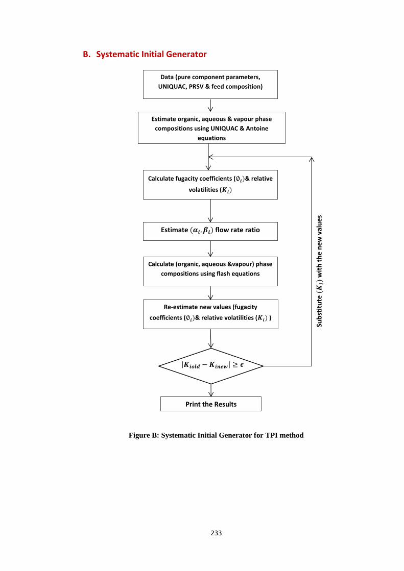
233
Systematic Initial Generator B.
Figure B: Systematic Initial Generator for TPI method
Data (pure component parameters,
UNIQUAC, PRSV & feed composition)
Re-estimate new values (fugacity
coefficients (∅𝒊)& relative volatilities (𝑲𝒊) )
Calculate (organic, aqueous &vapour) phase
compositions using flash equations
Calculate fugacity coefficients (∅𝒊)& relative
volatilities (𝑲𝒊)
Estimate (𝜶𝒊,𝜷𝒊) flow rate ratio
Print the Results
|𝑲𝒊𝒐𝒍𝒅 − 𝑲𝒊𝒏𝒆𝒘| ≥ 𝝐
Sub
stit
ute
(𝑲𝒊)
wit
h t
he
new
val
ues
Estimate organic, aqueous & vapour phase
compositions using UNIQUAC & Antoine
equations
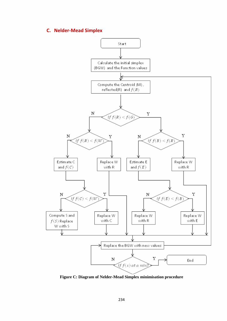
234
Nelder-Mead Simplex C.
Figure C: Diagram of Nelder-Mead Simplex minimisation procedure
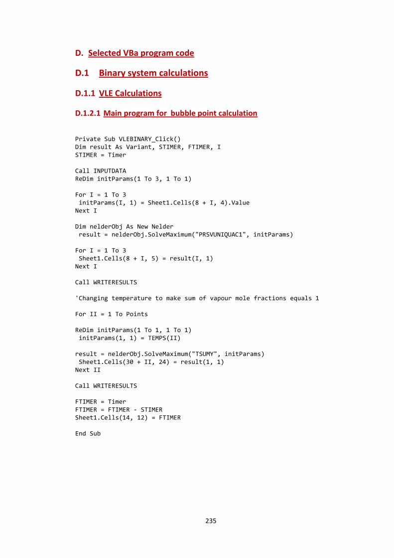
235
Selected VBa program code D.
D.1 Binary system calculations
D.1.1 VLE Calculations
Main program for bubble point calculation D.1.2.1
Private Sub VLEBINARY_Click() Dim result As Variant, STIMER, FTIMER, I STIMER = Timer Call INPUTDATA ReDim initParams(1 To 3, 1 To 1) For I = 1 To 3 initParams(I, 1) = Sheet1.Cells(8 + I, 4).Value Next I Dim nelderObj As New Nelder result = nelderObj.SolveMaximum("PRSVUNIQUAC1", initParams) For I = 1 To 3 Sheet1.Cells(8 + I, 5) = result(I, 1) Next I Call WRITERESULTS 'Changing temperature to make sum of vapour mole fractions equals 1 For II = 1 To Points ReDim initParams(1 To 1, 1 To 1) initParams(1, 1) = TEMPS(II) result = nelderObj.SolveMaximum("TSUMY", initParams) Sheet1.Cells(30 + II, 24) = result(1, 1) Next II Call WRITERESULTS FTIMER = Timer FTIMER = FTIMER - STIMER Sheet1.Cells(14, 12) = FTIMER End Sub
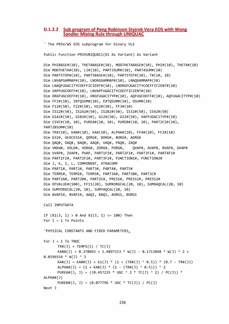
236
Sub program of Peng Robinson Styjrek Vera EOS with Wong D.1.2.2Sandler Mixing Rule through UNIQUAC
' The PRSV/WS EOS subprogram for binary VLE
Public Function PRSVUNIQUAC1(X1 As Variant) As Variant
Dim PHIBASE#(10), THETABASE#(10), MODTHETABASE#(10), PHI#(10), THETA#(10)
Dim MODTHETA#(10), LI#(10), PART3SUM#(10), PART4SUM#(10)
Dim PART5TOP#(10), PART5BASE#(10), PART5TOT#(10), T#(10, 10)
Dim LNVAPGAMMAP#(10), LNORGGAMMAP#(10), LNAQGAMMAP#(10)
Dim LNAQFUGACITYCOEFFICIENT#(10), LNORGFUGACITYCOEFFICIENT#(10)
Dim VAPFUGCOEFF#(10), LNVAPFUGACITYCOEFFICIENT#(10)
Dim ORGFUGCOEFF#(10), ORGFUGACITYP#(10), AQFUGCOEFF#(10), AQFUGACITYP#(10)
Dim FF1#(10), INTQSUM#(10), EXTQSUM#(10), DSUM#(10)
Dim F12#(50), F22#(50), H12#(50), FF3#(10)
Dim IS12#(50), IS2A2#(50), IS2B2#(50), IS32#(50), IS42#(50)
Dim G1A2#(50), G1B2#(50), G12#(50), G22#(50), VAPFUGACITYP#(10)
Dim CSVC#(10, 10), PUREA#(10, 10), PUREB#(10, 10), PART2C1#(10),
PART2BSUM#(10)
Dim TR#(10), KA0#(10), KA#(10), ALPHA#(10), FF4#(10), FF2#(10)
Dim G32#, GEXCESS#, QORG#, DORG#, BORG#, AORG#
Dim QAQ#, DAQ#, BAQ#, AAQ#, VAQ#, PAQ#, ZAQ#
Dim VNEW#, VOLD#, VORG#, ZORG#, PORG#, QVAP#, AVAP#, BVAP#, DVAP#
Dim VVAP#, ZVAP#, PVAP, PART1F1#, PART2F1#, PART3F1#, PART4F1#
Dim PART1F2#, PART2F2#, PART3F2#, FUNCTION1#, FUNCTION2#
Dim J, K, I, L, COMPONENT, XTRACOMP
Dim PART1#, PART2#, PART3#, PART4#, PART5#
Dim TERM1#, TERM2#, TERM3#, PART3A#, PART3B#, PART3C#
Dim PART2A#, PART2B#, PART2C#, PRESS#, PRESS1#, PRESS2#
Dim OFVALUE#(100), FF11(20), SUMXORGCAL(20, 10), SUMXAQCAL(20, 10)
Dim SUMYORGCAL(20, 10), SUMYAQCAL(20, 10)
Dim AVAP1#, BVAP1#, AAQ1, BAQ1, AORG1, BORG1
Call INPUTDATA
If (X1(3, 1) > 0 And X1(3, 1) <= 100) Then
For I = 1 To Points
'PHYSICAL CONSTANTS AND FIXED PARAMETERS.
For J = 1 To TNOC
TR#(J) = TEMPS(I) / TC(J)
KA0#(J) = 0.378893 + 1.4897153 * W(J) - 0.1713848 * W(J) ^ 2 +
0.0196554 * W(J) ^ 3
KA#(J) = KA0#(J) + k1(J) * (1 + (TR#(J) ^ 0.5)) * (0.7 - TR#(J))
ALPHA#(J) = (1 + KA#(J) * (1 - (TR#(J) ^ 0.5))) ^ 2
PUREA#(J, J) = ((0.457235 * UGC ^ 2 * TC(J) ^ 2) / PC(J)) *
ALPHA#(J)
PUREB#(J, J) = (0.077796 * UGC * TC(J)) / PC(J)
Next J
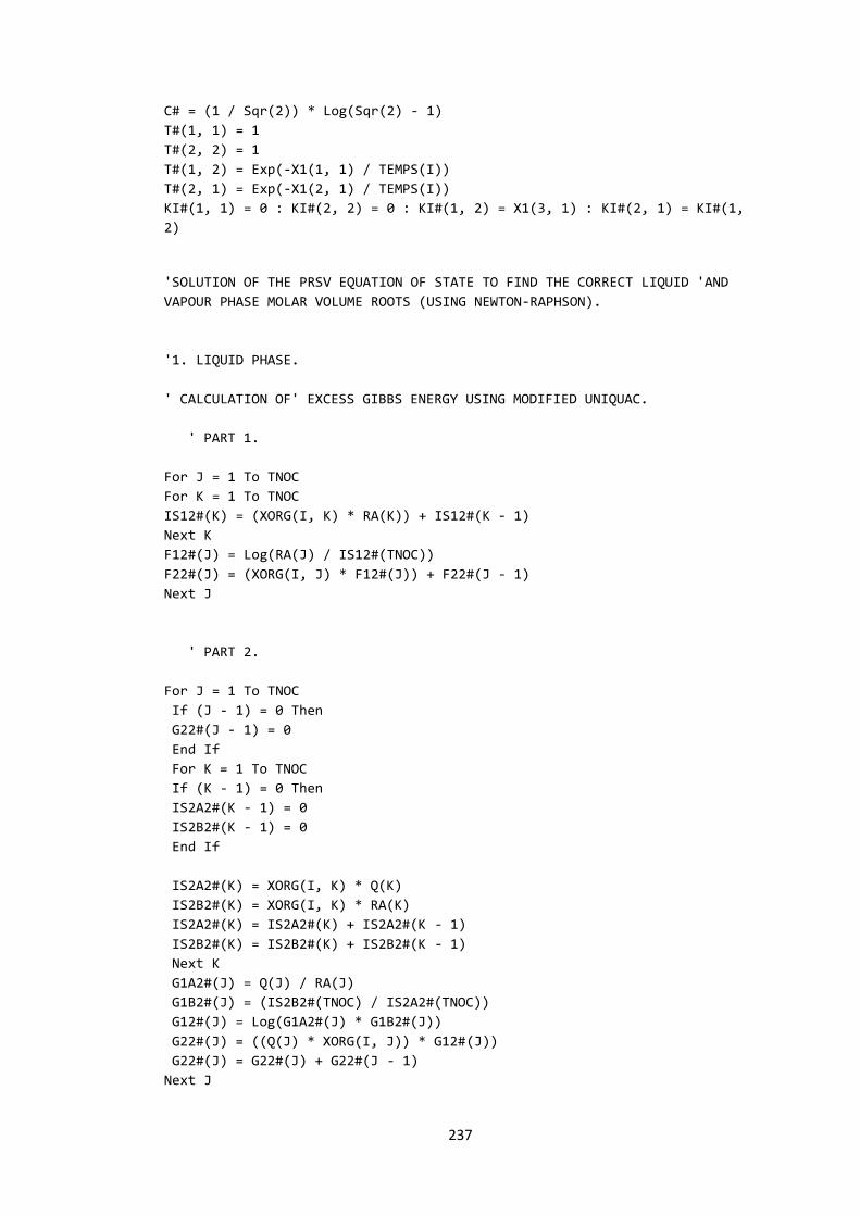
237
C# = (1 / Sqr(2)) * Log(Sqr(2) - 1)
T#(1, 1) = 1
T#(2, 2) = 1
T#(1, 2) = Exp(-X1(1, 1) / TEMPS(I))
T#(2, 1) = Exp(-X1(2, 1) / TEMPS(I))
KI#(1, 1) = 0 : KI#(2, 2) = 0 : KI#(1, 2) = X1(3, 1) : KI#(2, 1) = KI#(1,
2)
'SOLUTION OF THE PRSV EQUATION OF STATE TO FIND THE CORRECT LIQUID 'AND
VAPOUR PHASE MOLAR VOLUME ROOTS (USING NEWTON-RAPHSON).
'1. LIQUID PHASE.
' CALCULATION OF' EXCESS GIBBS ENERGY USING MODIFIED UNIQUAC.
' PART 1.
For J = 1 To TNOC
For K = 1 To TNOC
IS12#(K) = (XORG(I, K) * RA(K)) + IS12#(K - 1)
Next K
F12#(J) = Log(RA(J) / IS12#(TNOC))
F22#(J) = (XORG(I, J) * F12#(J)) + F22#(J - 1)
Next J
' PART 2.
For J = 1 To TNOC
If (J - 1) = 0 Then
G22#(J - 1) = 0
End If
For K = 1 To TNOC
If (K - 1) = 0 Then
IS2A2#(K - 1) = 0
IS2B2#(K - 1) = 0
End If
IS2A2#(K) = XORG(I, K) * Q(K)
IS2B2#(K) = XORG(I, K) * RA(K)
IS2A2#(K) = IS2A2#(K) + IS2A2#(K - 1)
IS2B2#(K) = IS2B2#(K) + IS2B2#(K - 1)
Next K
G1A2#(J) = Q(J) / RA(J)
G1B2#(J) = (IS2B2#(TNOC) / IS2A2#(TNOC))
G12#(J) = Log(G1A2#(J) * G1B2#(J))
G22#(J) = ((Q(J) * XORG(I, J)) * G12#(J))
G22#(J) = G22#(J) + G22#(J - 1)
Next J
238
G32# = (Z / 2) * G22#(TNOC)
' PART 3.
For J = 1 To TNOC
If (J - 1) = 0 Then
H12#(J - 1) = 0
End If
For K = 1 To TNOC
If (K - 1) = 0 Then
IS32#(K - 1) = 0
End If
For L = 1 To TNOC
If (L - 1) = 0 Then
IS42#(L - 1) = 0
End If
IS42#(L) = XORG(I, L) * QD(L)
IS42#(L) = IS42#(L) + IS42#(L - 1)
Next L
IS32#(K) = (XORG(I, K) * QD(K) * T#(K, J)) / IS42#(TNOC)
IS32#(K) = IS32#(K) + IS32#(K - 1)
Next K
H12#(J) = QD(J) * XORG(I, J) * (Log(IS32#(TNOC)))
H12#(J) = H12#(J) + H12#(J - 1)
Next J
GEXCESS# = F22#(TNOC) + G32# - H12#(TNOC)
'CALCULATION OF THE EXCLUDED VOLUME PARAMETER (bm).
For J = 1 To TNOC
For K = 1 To TNOC
CSVC#(J, K) = (((PUREB#(J, J) - (PUREA#(J, J) / (UGC * TEMPS(I)))) +
(PUREB#(K, K) - (PUREA#(K, K) / (UGC * TEMPS(I))))) / 2) * (1 - (KI#(J,
K) / 100))
Next K
Next J
For J = 1 To TNOC
For K = 1 To TNOC
INTQSUM#(K) = (XORG(I, J) * XORG(I, K) * CSVC#(J, K)) + INTQSUM#(K - 1)
Next K
EXTQSUM#(J) = INTQSUM#(TNOC) + EXTQSUM#(J - 1)
Next J
QORG# = EXTQSUM#(TNOC)
For J = 1 To TNOC
DSUM#(J) = ((XORG(I, J) * PUREA#(J, J)) / (PUREB#(J, J) * UGC *
TEMPS(I))) + DSUM#(J - 1)
Next J
DORG# = DSUM#(TNOC) + (GEXCESS# / C#)

239
BORG# = QORG# / (1 - DORG#)
'CALCULATION OF' THE ENERGY OF ATTRACTION PARAMETER (am) and
compressibility factor
AORG# = UGC * TEMPS(I) * BORG# * DORG#
AORG1 = AORG# * P / (UGC * TEMPS(I)) ^ 2
BORG1 = BORG# * P / (UGC * TEMPS(I))
ZORG# = Z3ROOT(AORG1, BORG1)
VORG# = ZORG# * (UGC * TEMPS(I)) / P
PORG = ((UGC * TEMPS(I)) / (VORG# - BORG#)) - (AORG# / (VORG# ^ 2 + (2 *
BORG# * VORG#) - BORG# ^ 2))
'2- VAPOUR-PHASE.
' CALCULATION OF EXCESS GIBBS ENERGY USING MODIFIED UNIQUAC.
' PART 1.
For K = 1 To TNOC
YEXP1(I, K) = (Exp(ANTA(K) - ANTB(K) / (ANTC(K) + TEMPS(I)))) / 750
YEXP1(I, K) = YEXP1(I, K) / P
YEXP1(I, K) = YEXP1(I, K) * XORG(I, K)
Next K
For J = 1 To TNOC
If (J - 1) = 0 Then
F22#(J - 1) = 0
End If
For K = 1 To TNOC
If (K - 1) = 0 Then
IS12#(K - 1) = 0
End If
IS12#(K) = YEXP1(I, K) * RA(K)
IS12#(K) = IS12#(K - 1) + IS12#(K)
Next K
F12#(J) = Log(RA(J) / IS12#(TNOC))
F22#(J) = (YEXP1(I, J) * F12#(J)) + F22#(J - 1)
Next J
' PART 2.
For J = 1 To TNOC
If (J - 1) = 0 Then
G22#(J - 1) = 0
End If
For K = 1 To TNOC
If (K - 1) = 0 Then
IS2A2#(K - 1) = 0
IS2B2#(K - 1) = 0
End If
IS2A2#(K) = YEXP1(I, K) * Q(K)

240
IS2B2#(K) = YEXP1(I, K) * RA(K)
IS2A2#(K) = IS2A2#(K) + IS2A2#(K - 1)
IS2B2#(K) = IS2B2#(K) + IS2B2#(K - 1)
Next K
G1A2#(J) = Q(J) / RA(J)
G1B2#(J) = (IS2B2#(TNOC) / IS2A2#(TNOC))
G12#(J) = Log(G1A2#(J) * G1B2#(J))
G22#(J) = ((Q(J) * YEXP1(I, J)) * G12#(J))
G22#(J) = G22#(J) + G22#(J - 1)
Next J
G32# = (Z / 2) * G22#(TNOC)
' PART 3.
For J = 1 To TNOC
If (J - 1) = 0 Then
H12#(J - 1) = 0
End If
For K = 1 To TNOC
If (K - 1) = 0 Then
IS32#(K - 1) = 0
End If
For L = 1 To TNOC
If (L - 1) = 0 Then
IS42#(L - 1) = 0
End If
IS42#(L) = YEXP1(I, L) * QD(L)
IS42#(L) = IS42#(L) + IS42#(L - 1)
Next L
IS32#(K) = (YEXP1(I, K) * QD(K) * T#(K, J)) / IS42#(TNOC)
IS32#(K) = IS32#(K) + IS32#(K - 1)
Next K
H12#(J) = QD(J) * YEXP1(I, J) * (Log(IS32#(TNOC)))
H12#(J) = H12#(J) + H12#(J - 1)
Next J
GEXCESS# = F22#(TNOC) + G32# - H12#(TNOC)
'EXCLUDED VOLUME PARAMETER (bm).
For J = 1 To TNOC
For K = 1 To TNOC
CSVC#(J, K) = (((PUREB#(J, J) - (PUREA#(J, J) / (UGC * TEMPS(I)))) +
(PUREB#(K, K) _- (PUREA#(K, K) / (UGC * TEMPS(I))))) / 2) * (1 - (KI#(J,
K) / 100))
Next K
Next J
For J = 1 To TNOC
For K = 1 To TNOC
INTQSUM#(K) = (YEXP1(I, J) * YEXP1(I, K) * CSVC#(J, K)) + INTQSUM#(K - 1)
Next K
241
EXTQSUM#(J) = INTQSUM#(TNOC) + EXTQSUM#(J - 1)
Next J
QVAP# = EXTQSUM#(TNOC)
For J = 1 To TNOC
DSUM#(J) = (YEXP1(1, J) * (PUREA#(J, J) / (PUREB#(J, J) * UGC *
TEMPS(I)))) + DSUM#(J - 1)
Next J
DVAP# = (DSUM#(TNOC) + (GEXCESS# / C#))
BVAP# = QVAP# / (1 - DVAP#)
'ATTRACTIVE PARAMETER (am) and compressibility factor
AVAP# = UGC * TEMPS(I) * BVAP# * DVAP#
ZVAP# = (P * VVAP#) / (UGC * TEMPS(I))
AVAP1# = AVAP# * P / (UGC * TEMPS(I)) ^ 2
BVAP1# = BVAP# * P / (UGC * TEMPS(I))
ZVAP# = ZVROOT(AVAP1#, BVAP1#)
VVAP# = (ZVAP# * UGC * TEMPS(I)) / P
PVAP = ((UGC * TEMPS(I)) / (VVAP# - BVAP#)) - (AVAP# / (VVAP# ^ 2 + (2 *
BVAP# * VVAP#) - BVAP# ^ 2))
' DETERMINATION OF THE FUGAC1TY COEFFICIENTS OF EACH COMPONENT IN EACH
PHASE.
'1. LIQUID PHASE.
'CALCULATION OF THE LIQUID PHASE ACTIVITY COEFFICIENTS AFTHIS P & T.
' THE UNIQUAC EXPANSION (CALCULATION OF ACTIVITY COEFFICIENTS FOR EACH
' COMPONENT IN THE LIQUID PHASE).
For COMPONENT = 1 To TNOC
PHIBASE#(COMPONENT) = RA(COMPONENT) * XORG(I, COMPONENT) +
PHIBASE#(COMPONENT - 1)
THETABASE#(COMPONENT) = Q(COMPONENT) * XORG(I, COMPONENT) +
THETABASE#(COMPONENT - 1)
MODTHETABASE#(COMPONENT) = QD(COMPONENT) * XORG(I, COMPONENT) +
MODTHETABASE#(COMPONENT - 1)
Next COMPONENT
For COMPONENT = 1 To TNOC
PHI#(COMPONENT) = (RA(COMPONENT) * XORG(I, COMPONENT)) / PHIBASE#(TNOC)
THETA#(COMPONENT) = (Q(COMPONENT) * XORG(I, COMPONENT)) / THETABASE#(TNOC)
MODTHETA#(COMPONENT) = (QD(COMPONENT) * XORG(I, COMPONENT)) /
MODTHETABASE(TNOC)
Next COMPONENT
242
For COMPONENT = 1 To TNOC
LI#(COMPONENT) = (Z / 2) * (RA(COMPONENT) - Q(COMPONENT)) -
(RA(COMPONENT) - 1)
Next COMPONENT
For COMPONENT = 1 To TNOC
PART1# = Log(PHI#(COMPONENT) / XORG(I, COMPONENT))
PART2# = (Z / 2) * Q(COMPONENT) * Log(THETA#(COMPONENT) /
PHI#(COMPONENT))
For J = 1 To TNOC
PART3SUM#(J) = XORG(I, J) * LI#(J) + PART3SUM#(J - 1)
PART4SUM#(J) = MODTHETA#(J) * T#(J, COMPONENT) + PART4SUM#(J - 1)
Next J
PART3# = (PHI#(COMPONENT) / XORG(I, COMPONENT)) * PART3SUM#(TNOC)
PART4# = QD(COMPONENT) * Log(PART4SUM#(TNOC))
For J = 1 To TNOC
PART5TOP#(J) = MODTHETA#(J) * T#(COMPONENT, J)
For K = 1 To TNOC
PART5BASE#(K) = MODTHETA#(K) * T#(K, J) + PART5BASE#(K - 1)
Next K
PART5TOT#(J) = (PART5TOP#(J) / PART5BASE#(TNOC)) + PART5TOT#(J - 1)
Next J
PART5# = QD(COMPONENT) * PART5TOT#(TNOC)
LNORGGAMMAP#(COMPONENT) = PART1# + PART2# + LI#(COMPONENT) - PART3# -
PART4# + QD(COMPONENT) - PART5#
Next COMPONENT
For XTRACOMP = 1 To TNOC
TERM1# = -Log((P * (VORG# - BORG#)) / (UGC * TEMPS(I)))
For J = 1 To TNOC
PART2BSUM#(J) = (XORG(I, J) * CSVC#(XTRACOMP, J)) + PART2BSUM#(J - 1)
Next J
PART2B# = (1 / (1 - DORG#)) * (2 * PART2BSUM#(TNOC))
PART2C1#(XTRACOMP) = ((PUREA#(XTRACOMP, XTRACOMP) / (PUREB#(XTRACOMP,
XTRACOMP) * UGC * TEMPS(I))) + (LNORGGAMMAP#(XTRACOMP) / C#))
PART2C# = (QORG# / ((1 - DORG#) ^ 2)) * (1 - PART2C1#(XTRACOMP))
PART2A# = PART2B# - PART2C#
TERM2# = (1 / BORG#) * PART2A# * (((P * VORG#) / (UGC * TEMPS(I))) - 1)
PART3A# = (1 / (2 * Sqr(2))) * (AORG# / (BORG# * UGC * TEMPS(I)))
PART3B# = ((((UGC * TEMPS(I) * DORG#) / AORG#) - (1 / BORG#)) * PART2A# +
((UGC * TEMPS(I) * BORG#) / AORG#) * PART2C1(XTRACOMP))
PART3C# = Log((VORG# + BORG# * (1 - Sqr(2))) / (VORG# + BORG# * (1 +
Sqr(2))))
TERM3# = PART3A# * PART3B# * PART3C#
LNORGFUGACITYCOEFFICIENT#(XTRACOMP) = TERM1# + TERM2# + TERM3#
ORGFUGCOEFF#(XTRACOMP) = Exp(LNORGFUGACITYCOEFFICIENT#(XTRACOMP))
Next XTRACOMP

243
'2- VAPOUR PHASE.
'CALCULATION OFT HE LIQUID PHASE ACTIVITY COEFFICIENTS AT THIS P & T.
'THE UNIQUAC EXPANSION (CALCULATION OF ACTIVITY COEFFICIENTS FOR EACH
' COMPONENT IN THE LIQUID PHASE).
For COMPONENT = I To TNOC
PHIBASE#(COMPONENT) = RA(COMPONENT) * YEXP1(I, COMPONENT) +
PHIBASE#(COMPONENT - 1)
THETABASE#(COMPONENT) = Q(COMPONENT) * YEXP1(I, COMPONENT) +
THETABASE#(COMPONENT - 1)
MODTHETABASE#(COMPONENT) = QD(COMPONENT) * YEXP1(I, COMPONENT) +
MODTHETABASE#(COMPONENT - 1)
Next COMPONENT
For COMPONENT = 1 To TNOC
PHI#(COMPONENT) = (RA(COMPONENT) * YEXP1(I, COMPONENT)) / PHIBASE#(TNOC)
THETA#(COMPONENT) = (Q(COMPONENT) * YEXP1(I, COMPONENT)) /
THETABASE#(TNOC)
MODTHETA#(COMPONENT) = (QD(COMPONENT) * YEXP1(I, COMPONENT)) /
MODTHETABASE#(TNOC)
Next COMPONENT
For COMPONENT = 1 To TNOC
LI#(COMPONENT) = (Z / 2) * (RA(COMPONENT) - Q(COMPONENT)) - (RA(COMPONENT)
- 1)
Next COMPONENT
For COMPONENT = 1 To TNOC
PART1# = Log(PHI#(COMPONENT) / YEXP1(I, COMPONENT))
PART2# = (Z / 2) * Q(COMPONENT) * Log(THETA#(COMPONENT) / PHI#(COMPONENT))
For J = 1 To TNOC
PART3SUM#(J) = YEXP1(I, J) * LI#(J) + PART3SUM#(J - 1)
PART4SUM#(J) = MODTHETA#(J) * T#(J, COMPONENT) + PART4SUM#(J - 1)
Next J
PART3# = (PHI#(COMPONENT) / YEXP1(I, COMPONENT)) * PART3SUM#(TNOC)
PART4# = QD(COMPONENT) * Log(PART4SUM#(TNOC))
For J = 1 To TNOC
PART5TOP#(J) = MODTHETA#(J) * T#(COMPONENT, J)
For K = 1 To TNOC
PART5BASE#(K) = MODTHETA#(K) * T#(K, J) + PART5BASE#(K - 1)
Next K
PART5TOT#(J) = (PART5TOP#(J) / PART5BASE#(TNOC)) + PART5TOT#(J - 1)
Next J
PART5# = QD(COMPONENT) * PART5TOT#(TNOC)
LNVAPGAMMAP#(COMPONENT) = PART1# + PART2# + LI#(COMPONENT) - PART3# -
PART4# + QD(COMPONENT) - PART5#
Next COMPONENT
For XTRACOMP = 1 To TNOC

244
TERM1# = -Log((P * (VVAP# - BVAP#)) / (UGC * TEMPS(I)))
For J = 1 To TNOC
PART2BSUM#(J) = (YEXP1(I, J) * CSVC#(XTRACOMP, J)) + PART2BSUM#(J - 1)
Next J
PART2B# = (1 / (1 - DVAP#)) * (2 * PART2BSUM#(TNOC))
PART2C1#(XTRACOMP) = ((PUREA#(XTRACOMP, XTRACOMP) / (PUREB#(XTRACOMP,
XTRACOMP) * UGC * TEMPS(I))) + (LNVAPGAMMAP#(XTRACOMP) / C#))
PART2C# = (QVAP# / (1 - DVAP#) ^ 2) * (1 - PART2C1#(XTRACOMP))
PART2A# = PART2B# - PART2C#
TERM2# = (1 / BVAP#) * PART2A# * (((P * VVAP#) / (UGC * TEMPS(I))) - 1)
PART3A# = (1 / (2 * Sqr(2))) * (AVAP# / (BVAP# * UGC * TEMPS(I)))
PART3B# = ((((UGC * TEMPS(I) * DVAP#) / AVAP#) - (1 / BVAP#)) * PART2A# +
((UGC * TEMPS(I) * BVAP#) / AVAP#) * PART2C1#(XTRACOMP))
PART3C# = Log((VVAP# + BVAP# * (1 - Sqr(2))) / (VVAP# + BVAP# * (1 +
Sqr(2))))
TERM3# = PART3A# * PART3B# * PART3C#
LNVAPFUGACITYCOEFFICIENT#(XTRACOMP) = TERM1# + TERM2# + TERM3#
VAPFUGCOEFF#(XTRACOMP) = Exp(LNVAPFUGACITYCOEFFICIENT#(XTRACOMP))
Next XTRACOMP
'CALCULATION OF THE OBECTIVE FUNCTION.
For COMPONENT = 1 To TNOC
ORGFUGACITYP#(COMPONENT) = ORGFUGCOEFF#(COMPONENT) * XORG(I, COMPONENT)
VAPFUGACITYP#(COMPONENT) = VAPFUGCOEFF#(COMPONENT) * YEXP1(I, COMPONENT)
YORGCAL(I, COMPONENT) = ORGFUGACITYP#(COMPONENT) /
VAPFUGCOEFF#(COMPONENT)
SUMYORGCAL(I, COMPONENT) = YORGCAL(I, COMPONENT) + SUMYORGCAL(I,
(COMPONENT - 1))
Sheet1.Cells(30 + I, COMPONENT + 30) = ORGFUGCOEFF#(COMPONENT)
Sheet1.Cells(30 + I, COMPONENT + 33) = VAPFUGCOEFF#(COMPONENT)
Next COMPONENT
For COMPONENT = 1 To (TNOC)
FF1#(COMPONENT) = Abs(YORGCAL(I, COMPONENT) - YEXP(I, COMPONENT)) +
FF1#(COMPONENT - 1)
Next COMPONENT
OFVALUE#(I) = FF1#(TNOC) + OFVALUE#(I - 1)
Next I
PRSVUNIQUAC1 = (OFVALUE#(Points) / (Points * TNOC)) * 1
Else
PRSVUNIQUAC1 = 100000
End If
Sheet1.Cells(9, 9) = PRSVUNIQUAC1
End Function

245
D.1.2 Area Method main program for binary LLE
Area Method main program for binary LLE D.1.2.1
Private Sub AreaMethod_Click()
Dim GMIXING, FAXA, FAXB, N, XA, XB
Dim XA22 As Double: Dim XB22 As Double
Dim start, finish
start = Timer
N = 100
AreaMax = -100000
‘Input the pure component properties for PRSV and UNIQUAC and the
interaction parameters
Call INPUTDATA
' Opening two “for-next” loops to search the entire composition &
estimating Gibbs energy at each point
For XA = 0.001 To 0.99 Step 0.001
XA22 = XA
Call PHICALCL(XA, GMIXING)
FAXA = GMIXING
For XB = 0.99 To XA Step -0.005
XB22 = XB
Call PHICALCL(XB, GMIXING)
FAXB = GMIXING
' Integration of the area under Gibbs free energy curve between XA & XB &
the string No.
INTEGRATION = IntegrateSimpson.Simpson(XA22, XB22, 100)
'Calculating the Maximum Positive Net Area M.P.N.A
AREA = Abs((FAXA + FAXB) * (XB - XA) / 2) - Abs(INTEGRATION)
'Searching for the M.P.N.A.
If AREA >= AreaMax Then
AreaMax = AREA
XAMax = XA
XBMax = XB
End If
Next XB
Next XA
'Finishing & writing the results to the sheet
finish = Timer
Sheet2.Cells(11, 19) = XAMax
Sheet2.Cells(11, 20) = XBMax
Sheet2.Cells(11, 18) = AreaMax
Sheet2.Cells(11, 21) = finish - start
End Sub
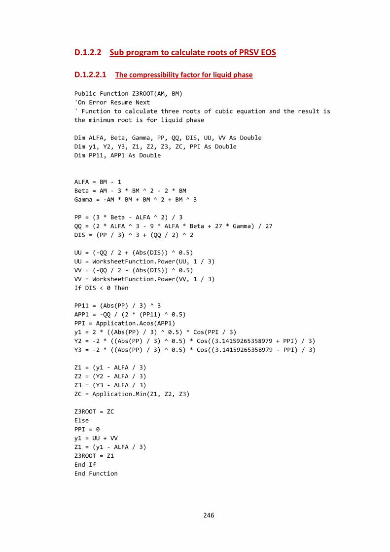
246
Sub program to calculate roots of PRSV EOS D.1.2.2
D.1.2.2.1 The compressibility factor for liquid phase
Public Function Z3ROOT(AM, BM)
'On Error Resume Next
' Function to calculate three roots of cubic equation and the result is
the minimum root is for liquid phase
Dim ALFA, Beta, Gamma, PP, QQ, DIS, UU, VV As Double
Dim y1, Y2, Y3, Z1, Z2, Z3, ZC, PPI As Double
Dim PP11, APP1 As Double
ALFA = BM - 1
Beta = AM - 3 * BM ^ 2 - 2 * BM
Gamma = -AM * BM + BM ^ 2 + BM ^ 3
PP = (3 * Beta - ALFA ^ 2) / 3
QQ = (2 * ALFA ^ 3 - 9 * ALFA * Beta + 27 * Gamma) / 27
DIS = (PP / 3) ^ 3 + (QQ / 2) ^ 2
UU = (-QQ / 2 + (Abs(DIS)) ^ 0.5)
UU = WorksheetFunction.Power(UU, 1 / 3)
VV = (-QQ / 2 - (Abs(DIS)) ^ 0.5)
VV = WorksheetFunction.Power(VV, 1 / 3)
If DIS < 0 Then
PP11 = (Abs(PP) / 3) ^ 3
APP1 = -QQ / (2 * (PP11) ^ 0.5)
PPI = Application.Acos(APP1)
y1 = 2 * ((Abs(PP) / 3) ^ 0.5) * Cos(PPI / 3)
Y2 = -2 * ((Abs(PP) / 3) ^ 0.5) * Cos((3.14159265358979 + PPI) / 3)
Y3 = -2 * ((Abs(PP) / 3) ^ 0.5) * Cos((3.14159265358979 - PPI) / 3)
Z1 = (y1 - ALFA / 3)
Z2 = (Y2 - ALFA / 3)
Z3 = (Y3 - ALFA / 3)
ZC = Application.Min(Z1, Z2, Z3)
Z3ROOT = ZC
Else
PPI = 0
y1 = UU + VV
Z1 = (y1 - ALFA / 3)
Z3ROOT = Z1
End If
End Function

247
D.1.2.2.2 The compressibility factor for Vapour Phase
Public Function ZVROOT(AM, BM)
' Function to calculate three roots of cubic equation and the result is
the maximum root is selected for vapour phase.
Dim ALFA, Beta, Gamma, PP, QQ, DIS, UU, VV As Double
Dim y1, Y2, Y3, Z1, Z2, Z3, ZC, PPI As Double
Dim PP11, APP1 As Double
ALFA = BM - 1
Beta = AM - 3 * BM ^ 2 - 2 * BM
Gamma = -AM * BM + BM ^ 2 + BM ^ 3
PP = (3 * Beta - ALFA ^ 2) / 3
QQ = (2 * ALFA ^ 3 - 9 * ALFA * Beta + 27 * Gamma) / 27
DIS = (PP / 3) ^ 3 + (QQ / 2) ^ 2
UU = (-QQ / 2 + (Abs(DIS)) ^ 0.5)
UU = WorksheetFunction.Power(UU, 1 / 3)
VV = (-QQ / 2 - (Abs(DIS)) ^ 0.5)
VV = WorksheetFunction.Power(VV, 1 / 3)
If DIS < 0 Then
PP11 = (Abs(PP) / 3) ^ 3
APP1 = -QQ / (2 * (PP11) ^ 0.5)
PPI = Application.Acos(APP1)
y1 = 2 * ((Abs(PP) / 3) ^ 0.5) * Cos(PPI / 3)
Y2 = -2 * ((Abs(PP) / 3) ^ 0.5) * Cos((3.14159265358979 + PPI) / 3)
Y3 = -2 * ((Abs(PP) / 3) ^ 0.5) * Cos((3.14159265358979 - PPI) / 3)
Z1 = (y1 - ALFA / 3)
Z2 = (Y2 - ALFA / 3)
Z3 = (Y3 - ALFA / 3)
ZC = Application.Max(Z1, Z2, Z3)
ZVROOT = ZC
Else
PPI = 0
y1 = UU + VV
Z1 = (y1 - ALFA / 3)
ZVROOT = Z1
End If
End Function

248
Calculation of pure component Gibbs free energy D.1.2.3
Public Sub PUREGCALC()
' Calculation of pure component Gibbs free energy at constant T& P.
Dim LOWPUREMIXG#(10), PUREV#(10, 10), TR#(10), K0#(10), K
Dim ALPHA#(10), KC#(10), GPURE1#(10, 10), GPURE2#(10, 10), GPURE3A#(10,
10), GPURE3B#(10, 10)
Dim DSUM#(10), PUREGSUM(10), GPURE3#(10, 10), GPURE4#(10, 10)
Dim J, CSVC1#, CSVC2#
Dim VNEW#, VCOUNT, VOLD#, PART1F1#, PART2F1#, PART3F1#, PART4F1#
Dim FUNCTION1#, FUNCTION2#, PART1F2#, PART2F2#, PART3F2#
Dim i, ZPP#, AP#, BP#
'CALCULATION OF PRSV EOS PURE COMPONENT PARAMETERS Ai AND Bi.
For J = 1 To TNOC
TR#(J) = TEMP / TC(J)
K0#(J) = 0.378893 + (1.4897153 * W(J)) - (0.17131848 * W(J) ^ 2) +
(0.0196554 * W(J) ^ 3)
KC#(J) = K0#(J) + (k1(J) * ((1 + Sqr(TR#(J))) * (0.7 - TR#(J))))
ALPHA#(J) = (1 + (KC#(J) * (1 - Sqr(TR#(J))))) ^ 2
PUREA#(J) = (((0.457235 * UGC ^ 2 * TC(J) ^ 2) / PC(J)) * ALPHA#(J))
PUREB#(J) = (0.077796 * UGC * TC(J)) / PC(J)
Next J
'CROSS SECOND VIRIAL COEFFICIENT CALCULATION.
For J = 1 To TNOC
For K = 1 To TNOC
CSVC1# = PUREB#(J) - (PUREA#(J) / (UGC * TEMP))
CSVC2# = PUREB#(K) - (PUREA#(K) / (UGC * TEMP))
CSVC#(J, K) = ((CSVC1# + CSVC2#) / 2) * (1 - KX#(J, K))
Next K
Next J
'CALCULATION OF THE PURE COMPONENT MOLAR VOLUMES AND GIBBS FREE ENERGIES
(AT FIXED T AND P)
' FOR EACH ROOT OF THE PRSV EOS. Newton–Raphson method is used
For J = 1 To 2
For K = 1 To TNOC
VNEW# = INITIALV#(J)
VCOUNT = 0
Do
VCOUNT = VCOUNT + 1

249
VOLD# = VNEW#
PART1F1# = P * (VOLD# ^ 3)
PART2F1# = ((P * PUREB#(K)) - (UGC * TEMP)) * VOLD# ^ 2
PART3F1# = ((3 * P * (PUREB#(K) ^ 2)) + (2 * UGC * TEMP * PUREB#(K)) -
PUREA#(K)) * VOLD#
PART4F1# = ((P * (PUREB#(K) ^ 3)) + (UGC * TEMP * (PUREB#(K) ^ 2)) -
(PUREA#(K) * PUREB#(K)))
FUNCTION1# = PART1F1# + PART2F1# - PART3F1# + PART4F1#
PART1F2# = 3 * P * (VOLD# ^ 2)
PART2F2# = 2 * ((P * PUREB#(K)) - (UGC * TEMP)) * VOLD#
PART3F2# = ((3 * P * (PUREB#(K) ^ 2)) + (2 * UGC * TEMP * PUREB#(K)) -
PUREA#(K))
FUNCTION2# = PART1F2# + PART2F2# - PART3F2#
VNEW# = VOLD# - (FUNCTION1# / FUNCTION2#)
If VCOUNT > 15 Then
GoTo VJUMP1
End If
Loop Until Abs(FUNCTION1#) < 1E-20
VJUMP1:
' OR the pure component molar volue can be estimated by calling the root
finder
AP# = PUREA#(K) * P / (UGC * TEMP) ^ 2
BP# = PUREB#(K) * P / (UGC * TEMP)
ZPP# = Z3ROOT(AP#, BP#)
VOLD# = (ZPP# * UGC * TEMP) / P
PUREV#(J, K) = VOLD#
GPURE1#(J, K) = (P * PUREV#(J, K)) / (UGC * TEMP)
GPURE2#(J, K) = Log(PUREV#(J, K) / (PUREV#(J, K) - PUREB#(K)))
GPURE3A#(J, K) = (PUREA#(K) / (2 * Sqr(2) * UGC * TEMP *
PUREB#(K)))
GPURE3B#(J, K) = (PUREV#(J, K) + ((1 - Sqr(2)) * PUREB#(K))) /
(PUREV#(J, K) + ((1 + Sqr(2)) * PUREB#(K)))
GPURE3#(J, K) = GPURE3A#(J, K) * Log(GPURE3B#(J, K))
'GPURE4#(J, K) = Log(100000! * (PUREV#(J, K) / (UGC * TEMP)))
GPURE4#(J, K) = Log((PUREV#(J, K) / (UGC * TEMP)))
PURECOMPG#(J, K) = GPURE1#(J, K) + GPURE2#(J, K) + GPURE3#(J,
K) - GPURE4#(J, K)
Next K
Next J
End Sub

250
Calculation of Gibbs free energy for the mixture D.1.2.4
Public Sub PHICALCL(x1, GMIXING)
Dim F12#(10), F22#(10), H12#(10)
Dim IS12#(10), IS2A2#(10), IS2B2#(10), IS32#(10), IS42#(10)
Dim G1A2#(10), G1B2#(10), G12#(10), G22#(10)
Dim T#(10, 10), TR#(10), K0#(10), KC#(10)
'Dim X(10), MIXTV#(10), ALPHA#(10), INTQSUM#(10), EXTQSUM#(10)
Dim MIXTV#(10), ALPHA#(10), INTQSUM#(10), EXTQSUM#(10)
Dim DSUM#(10), GPART1#(10), GPART2#(10), GPART3A#(10)
Dim GPART4#(10, 10), MIXTUREG(10), RADANGLE#(3), GPART3B#(10)
Dim GPART3#(10), QP#, AP#, YEXP, GEXCESS#, Z, L, i, J, K, G32#
Dim D#, b#, VNEW#, VCOUNT, VOLD#
Dim PART1F1#, PART2F1#, PART3F1#, PART4F1#
Dim FUNCTION1#, FUNCTION2#
Dim PART1F2#, PART2F2#, PART3F2#, PUREGMIX, LOWMIXG, LOWG
'Dim GMIXING, APV#
Dim APV#:Dim ZP#, BP#
Call PUREGCALC
'CALCULATION OF EXCESS GIBBS ENERGY USING MODIFIED UNIQUAC.
CX# = (1 / Sqr(2)) * Log(Sqr(2) - 1)
GEXCESS# = 0
For J = 1 To TNOC
For K = 1 To TNOC
IS12#(K) = (x(K) * R(K)) + IS12#(K - 1)
Next K
F12#(J) = Log(R(J) / IS12#(TNOC))
F22#(J) = (x(J) * F12#(J)) + F22#(J - 1)
Next J
For J = 1 To TNOC
For K = 1 To TNOC
IS2A2#(K) = (x(K) * Q(K)) + IS2A2#(K - 1)
IS2B2#(K) = (x(K) * R(K)) + IS2B2#(K - 1)
Next K
G1A2#(J) = Q(J) / R(J)
G1B2#(J) = (IS2B2#(TNOC) / IS2A2#(TNOC))
G12#(J) = Log(G1A2#(J) * G1B2#(J))
G22#(J) = ((Q(J) * x(J)) * G12#(J)) + G22#(J - 1)
Next J
G32# = (ZPAC / 2) * G22#(TNOC)
For J = 1 To TNOC
For K = 1 To TNOC
251
For L = 1 To TNOC
IS42#(L) = (x(L) * QD(L)) + IS42#(L - 1)
Next L
T#(K, J) = Exp(-AX#(K, J) / TEMP)
IS32#(K) = ((x(K) * QD(K) * T#(K, J)) / IS42#(TNOC)) + IS32#(K - 1)
Next K
H12#(J) = (QD(J) * x(J) * (Log(IS32#(TNOC)))) + H12#(J - 1)
Next J
GEXCESS# = F22#(TNOC) + G32# - H12#(TNOC)
'CALCULATION OF THE EXCLUDED VOLUME PARAMETER (BM).
For J = 1 To TNOC
For K = 1 To TNOC
INTQSUM#(K) = (x(J) * x(K) * CSVC#(J, K)) + INTQSUM#(K - 1)
Next K
EXTQSUM#(J) = INTQSUM#(TNOC) + EXTQSUM#(J - 1)
Next J
QP# = EXTQSUM#(TNOC)
For J = 1 To TNOC
DSUM#(J) = ((x(J) * PUREA#(J)) / (PUREB#(J) * UGC * TEMP)) + DSUM#(J - 1)
Next J
D# = DSUM#(TNOC) + (GEXCESS# / CX#)
b# = QP# / (1 - D#)
'CALCULATION OF THE ENERGY OF ATTRACTION PARAMETER (am).
AP# = (UGC * TEMP * b# * D#)
BP# = b# * P / (UGC * TEMP)
'CALCULATION OF THE MOLAR VOLUMES (AT FIXED T AND P), FOR EACH ROOT OF THE
PRSV EOS.
For J = 1 To 2 Step 1
VNEW# = INITIALV#(J)
VCOUNT = 0
Do
VCOUNT = VCOUNT + 1
VOLD# = VNEW#
PART1F1# = P * VOLD# ^ 3
PART2F1# = ((P * b#) - (UGC * TEMP)) * VOLD# ^ 2
PART3F1# = ((3 * P * (b# ^ 2)) + (2 * UGC * TEMP * b#) - AP#) * VOLD#
PART4F1# = ((P * (b# ^ 3)) + (UGC * TEMP * (b# ^ 2)) - (AP# * b#))
FUNCTION1# = PART1F1# + PART2F1# - PART3F1# + PART4F1#
PART1F2# = 3 * P * VOLD# ^ 2
PART2F2# = 2 * ((P * b#) - (UGC * TEMP)) * VOLD#
PART3F2# = ((3 * P * (b# ^ 2)) + (2 * UGC * TEMP * b#) - AP#)
FUNCTION2# = PART1F2# + PART2F2# - PART3F2#

252
VNEW# = VOLD# - (FUNCTION1# / FUNCTION2#)
If VCOUNT > 15 Then
GoTo VJUMP2
End If
Loop Until Abs(FUNCTION1#) < 1E-20
VJUMP2:
MIXTV#(J) = VOLD#
APV# = AP# * P / (UGC * TEMP) ^ 2
ZP# = Z3ROOT(APV#, BP#)
MIXTV#(J) = (ZP# * UGC * TEMP) / P
VOLML = Log(MIXTV#(J) * 10 ^ (-6))
'CALCULATION OF DIMENSIONLESS MIXTURE GIBBS FREE ENERGY.
GPART1#(J) = (P * MIXTV#(J)) / (UGC * TEMP)
GPART2#(J) = Log(MIXTV#(J) / (MIXTV#(J) - b#))
GPART3A#(J) = (AP# / (2 * Sqr(2) * UGC * TEMP * b#))
GPART3B#(J) = (MIXTV#(J) + ((1 - Sqr(2)) * b#)) / (MIXTV#(J) + ((1 +
Sqr(2)) * b#))
GPART3#(J) = GPART3A#(J) * Log(GPART3B#(J))
For K = 1 To TNOC
GPART4#(J, K) = (x(K) * Log((MIXTV#(J) / (x(K) * UGC * TEMP)))) +
GPART4#(J, K - 1)
Next K
MIXTUREG(J) = GPART1#(J) + GPART2#(J) + GPART3#(J) - GPART4#(J, TNOC)
Next J
PUREGMIX = 0
For i = 1 To TNOC
PUREGMIX = PUREGMIX + PURECOMPG#(1, i) * x(i)
Next i
PUREGMIX = PUREGMIX + PUREGINT
LOWMIXG = MIXTUREG(1)
LOWG = MIXTUREG(1) - PUREGMIX
If MIXTUREG(2) < LOWMIXG Then
LOWMIXG = MIXTUREG(2)
LOWG = MIXTUREG(2) - PUREGMIX
End If
GMIXING = LOWG
End Sub

253
Integration of Gibbs free energy curve using Simpson's rule D.1.2.5
Function Simpson(a As Double, b As Double, N As Integer) As Double
'n should be an even number
Dim J As Integer, s1 As Double, s2 As Double, h As Single
h = (b - a) / N
s1 = 0
s2 = 0
For J = 1 To N - 1 Step 2
s1 = s1 + f(a + J * h)
Next J
For J = 2 To N - 2 Step 2
s2 = s2 + f(a + J * h)
Next J
Simpson = h / 3 * (f(a) + 4 * s1 + 2 * s2 + f(b))
End Function
‘The Function code (f) is the same as PHICALCL
-------------------------------------------------------------------------------------------------------------------------------------
254
D.1.3 TPI for VLLE binary systems
D.1.3.1 Main program
Private Sub CommandButton2_Click()
Dim Z, GMIXINGV, GMIXING
Call INPUTDATA
Dim RESULT
' Gibbs free energy estimation at each grid considering the phase change
x(1) = -((1 / YLIM) / 2)
For Z = 1 To YLIM
x(1) = x(1) + 1 / YLIM
Call PHICALCL(x, GMIXING)
Call PHICALCV(x, GMIXINGV)
If GMIXINGV > GMIXING Then
GMIXINGF(Z) = GMIXING
VOLUME(Z) = VOLML
Else: GMIXINGF(Z) = GMIXINGV
VOLUME(Z) = VOLMV
End If
' Writting the results back to the sheet
Sheet1.Cells(3 + Z, 2) = x(1)
XXJ(Z) = x(1)
Sheet1.Cells(3 + Z, 3) = GMIXINGF(Z)
Sheet1.Cells(3 + Z, 4) = VOLUME(Z)
Next Z
' Calling the Nelder Mead Module to minimize the tau function
' Calculating the starting values
ReDim initParams(1 To 2, 1 To 1)
'initial values for XA & XB optimization
initParams(1, 1) = ZALFA - (1 / XGRID) * 2 ^ 0.5
initParams(2, 1) = 1 - (1 / XGRID) * 2 ^ 0.5 - ZALFA
Dim nelderObj As New Nelder
RESULT = nelderObj.SolveMaximum("fn", initParams)
Sheets("sheet2").Range("G12").Value = RESULT(1, 1)
Sheets("sheet2").Range("H12").Value = RESULT(2, 1)
' calling the Nelder Mead for the second time and with new starting
points
ReDim initParams(1 To 2, 1 To 1)

255
initParams(1, 1) = ZALFA - ((1 / XGRID) * 2 ^ 0.5) - XAH / 2
initParams(2, 1) = 1 - (1 / XGRID) * 2 ^ 0.5 - ZALFA
'Dim nelderObj As New Nelder
RESULT = nelderObj.SolveMaximum("fn", initParams)
Sheets("sheet2").Range("I12").Value = RESULT(1, 1)
Sheets("sheet2").Range("J12").Value = RESULT(2, 1)
End Sub
D.1.3.2 Sub procedure to calculate pure component Gibbs free energy
Public Sub PUREGCALC()
Dim LOWPUREMIXG#(10), PUREV#(10, 10), TR#(10), K0#(10), K
Dim ALPHA#(10), KC#(10), GPURE1#(10, 10), GPURE2#(10, 10), GPURE3A#(10,
10), GPURE3B#(10, 10)
Dim DSUM#(10), PUREGSUM(10), GPURE3#(10, 10), GPURE4#(10, 10)
Dim J, CSVC1#, CSVC2#
Dim VNEW#, VCOUNT, VOLD#, PART1F1#, PART2F1#, PART3F1#, PART4F1#
Dim FUNCTION1#, FUNCTION2#, PART1F2#, PART2F2#, PART3F2#
Dim I, ZPP#, AP#, BP#
'CALCULATION OF PRSV EOS PURE COMPONENT PARAMETERS Ai AND Bi.
For J = 1 To TNOC
TR#(J) = TEMP / TC(J)
K0#(J) = 0.378893 + (1.4897153 * W(J)) - (0.17131848 * W(J) ^ 2) +
(0.0196554 * W(J) ^ 3)
KC#(J) = K0#(J) + (k1(J) * ((1 + Sqr(TR#(J))) * (0.7 - TR#(J))))
ALPHA#(J) = (1 + (KC#(J) * (1 - Sqr(TR#(J))))) ^ 2
PUREA#(J) = (((0.457235 * UGC ^ 2 * TC(J) ^ 2) / PC(J)) * ALPHA#(J))
PUREB#(J) = (0.077796 * UGC * TC(J)) / PC(J)
Next J
'CROSS SECOND VIRIAL COEFFICIENT CALCULATION.
For J = 1 To TNOC
For K = 1 To TNOC
CSVC1# = PUREB#(J) - (PUREA#(J) / (UGC * TEMP))
CSVC2# = PUREB#(K) - (PUREA#(K) / (UGC * TEMP))
CSVC#(J, K) = ((CSVC1# + CSVC2#) / 2) * (1 - KX#(J, K))
Next K
Next J
'CALCULATION OF THE PURE COMPONENT MOLAR VOLUMES AND GIBBS FREE ENERGIES
(AT FIXED T AND P)
' FOR EACH ROOT OF THE PRSV EOS.
256
For J = 1 To 2
For K = 1 To TNOC
VNEW# = INITIALV#(J)
VCOUNT = 0
Do
VCOUNT = VCOUNT + 1
VOLD# = VNEW#
PART1F1# = P * (VOLD# ^ 3)
PART2F1# = ((P * PUREB#(K)) - (UGC * TEMP)) * VOLD# ^ 2
PART3F1# = ((3 * P * (PUREB#(K) ^ 2)) + (2 * UGC * TEMP * PUREB#(K))
- PUREA#(K)) * VOLD#
PART4F1# = ((P * (PUREB#(K) ^ 3)) + (UGC * TEMP * (PUREB#(K) ^ 2)) -
(PUREA#(K) * PUREB#(K)))
FUNCTION1# = PART1F1# + PART2F1# - PART3F1# + PART4F1#
PART1F2# = 3 * P * (VOLD# ^ 2)
PART2F2# = 2 * ((P * PUREB#(K)) - (UGC * TEMP)) * VOLD#
PART3F2# = ((3 * P * (PUREB#(K) ^ 2)) + (2 * UGC * TEMP * PUREB#(K))
- PUREA#(K))
FUNCTION2# = PART1F2# + PART2F2# - PART3F2#
VNEW# = VOLD# - (FUNCTION1# / FUNCTION2#)
If VCOUNT > 15 Then
GoTo VJUMP1
End If
Loop Until Abs(FUNCTION1#) < 1E-20
VJUMP1:
' AP# = PUREA#(K) * P / (UGC * TEMP) ^ 2
'BP# = PUREB#(K) * P / (UGC * TEMP)
'ZPP# = Z3ROOT(AP#, BP#)
'VOLD# = (ZPP# * UGC * TEMP) / P
PUREV#(J, K) = VOLD#
GPURE1#(J, K) = (P * PUREV#(J, K)) / (UGC * TEMP)
GPURE2#(J, K) = Log(PUREV#(J, K) / (PUREV#(J, K) - PUREB#(K)))
GPURE3A#(J, K) = (PUREA#(K) / (2 * Sqr(2) * UGC * TEMP * PUREB#(K)))
GPURE3B#(J, K) = (PUREV#(J, K) + ((1 - Sqr(2)) * PUREB#(K))) /
(PUREV#(J, K) + ((1 + Sqr(2)) * PUREB#(K)))
GPURE3#(J, K) = GPURE3A#(J, K) * Log(GPURE3B#(J, K))
'GPURE4#(J, K) = Log(100000! * (PUREV#(J, K) / (UGC * TEMP)))
GPURE4#(J, K) = Log((PUREV#(J, K) / (UGC * TEMP)))
PURECOMPG#(J, K) = GPURE1#(J, K) + GPURE2#(J, K) + GPURE3#(J, K) -
GPURE4#(J, K)
Next K
Next J
End Sub

257
D.1.3.3 Tau Objective Function
Public Function fn(x1 As Variant) As Variant
Dim XA(10), XB(10)
'CALCULATION FOR INITIAL VARIABLE VALUES(ALFA1,ALFA2)
XA(1) = ZALFA - x1(1, 1)
XA(2) = 1 - XA(1)
XB(1) = ZALFA + x1(2, 1)
XB(2) = 1 - XB(1)
If XA(1) > 0 And XA(1) < 1 And XB(1) > 0 And XB(1) < 1 Then
'CALCULATION FOR PURE COMPONENT GIBBS ENERGY PART2
Call PHICALCL(XA, GMIXING)
Call PHICALCV(XA, GMIXINGV)
If GMIXINGV > GMIXING Then
FAYXA = GMIXING
Else: FAYXA = GMIXINGV
End If
Call PHICALCL(XB, GMIXING)
Call PHICALCV(XB, GMIXINGV)
If GMIXINGV > GMIXING Then
FAYXB = GMIXING
Else: FAYXB = GMIXINGV
End If
'CALCULATION OF the tangent plane slope intercept and single delta tau
increment
fn = 0
TPS = (FAYXB - FAYXA) / (XB(1) - XA(1))
TPINT = FAYXA - (TPS * XA(1))
TPSCT = (1 / XGRID) * (1 + (TPS) ^ 2)
For J = 1 To XGRID
TPV = (TPS * XXJ(J)) + TPINT
If TPV > GMIXINGF(J) Then
fn = fn + TPSCT
End If
Next J
Else:
258
fn = 1000
End If
Sheet2.Cells(16, 9) = fn
XAL = ZALFA - x1(1, 1)
XAH = ZALFA + x1(2, 1)
End Function
D.1.3.4 Sub program of Gibbs free energy calculation for vapour phase
Public Sub PHICALCV(x, GMIXINGV)
Dim F12#(10), F22#(10), H12#(10)
Dim IS12#(10), IS2A2#(10), IS2B2#(10), IS32#(10), IS42#(10)
Dim G1A2#(10), G1B2#(10), G12#(10), G22#(10)
Dim T#(10, 10), TR#(10), K0#(10), KC#(10)
Dim MIXTV#(10), ALPHA#(10), INTQSUM#(10), EXTQSUM#(10)
Dim DSUM#(10), GPART1#(10), GPART2#(10), GPART3A#(10)
Dim GPART4#(10, 10), MIXTUREG(10), RADANGLE#(3), GPART3B#(10)
Dim GPART3#(10), QP#, AP#, YEXP, GEXCESS#, Z, L, I, J, K, G32#
Dim D#, B#, VNEW#, VCOUNT, VOLD#
Dim PART1F1#, PART2F1#, PART3F1#, PART4F1#
Dim FUNCTION1#, FUNCTION2#
Dim PART1F2#, PART2F2#, PART3F2#, PUREGMIX, LOWMIXG, LOWG
Dim APV#, ZP#, BP#
Call PUREGCALC
TPLIM = 0
x(2) = 1 - x(1)
'CALCULATION OF EXCESS GIBBS ENERGY USING MODIFIED UNIQUAC.
CX# = (1 / Sqr(2)) * Log(Sqr(2) - 1)
GEXCESS# = 0
For J = 1 To TNOC
For K = 1 To TNOC
IS12#(K) = (x(K) * R(K)) + IS12#(K - 1)
Next K
F12#(J) = Log(R(J) / IS12#(TNOC))
F22#(J) = (x(J) * F12#(J)) + F22#(J - 1)
Next J
For J = 1 To TNOC
For K = 1 To TNOC
IS2A2#(K) = (x(K) * Q(K)) + IS2A2#(K - 1)
IS2B2#(K) = (x(K) * R(K)) + IS2B2#(K - 1)
259
Next K
G1A2#(J) = Q(J) / R(J)
G1B2#(J) = (IS2B2#(TNOC) / IS2A2#(TNOC))
G12#(J) = Log(G1A2#(J) * G1B2#(J))
G22#(J) = ((Q(J) * x(J)) * G12#(J)) + G22#(J - 1)
Next J
G32# = (ZPAC / 2) * G22#(TNOC)
For J = 1 To TNOC
For K = 1 To TNOC
For L = 1 To TNOC
IS42#(L) = (x(L) * QD(L)) + IS42#(L - 1)
Next L
T#(K, J) = Exp(-AX#(K, J) / TEMP)
IS32#(K) = ((x(K) * QD(K) * T#(K, J)) / IS42#(TNOC)) + IS32#(K - 1)
Next K
H12#(J) = (QD(J) * x(J) * (Log(IS32#(TNOC)))) + H12#(J - 1)
Next J
GEXCESS# = F22#(TNOC) + G32# - H12#(TNOC)
'CALCULATION OF THE EXCLUDED VOLUME PARAMETER (BM).
For J = 1 To TNOC
For K = 1 To TNOC
INTQSUM#(K) = (x(J) * x(K) * CSVC#(J, K)) + INTQSUM#(K - 1)
Next K
EXTQSUM#(J) = INTQSUM#(TNOC) + EXTQSUM#(J - 1)
Next J
QP# = EXTQSUM#(TNOC)
For J = 1 To TNOC
DSUM#(J) = ((x(J) * PUREA#(J)) / (PUREB#(J) * UGC * TEMP)) + DSUM#(J - 1)
Next J
D# = DSUM#(TNOC) + (GEXCESS# / CX#)
B# = QP# / (1 - D#)
'CALCULATION OF THE ENERGY OF ATTRACTION PARAMETER (am).
AP# = (UGC * TEMP * B# * D#)
BP# = B# * P / (UGC * TEMP)
For J = 1 To 2 Step 1
VNEW# = INITIALV#(J)
VCOUNT = 0
Do
VCOUNT = VCOUNT + 1
VOLD# = VNEW#
PART1F1# = P * VOLD# ^ 3
PART2F1# = ((P * B#) - (UGC * TEMP)) * VOLD# ^ 2

260
PART3F1# = ((3 * P * (B# ^ 2)) + (2 * UGC * TEMP * B#) - AP#) * VOLD#
PART4F1# = ((P * (B# ^ 3)) + (UGC * TEMP * (B# ^ 2)) - (AP# * B#))
FUNCTION1# = PART1F1# + PART2F1# - PART3F1# + PART4F1#
PART1F2# = 3 * P * VOLD# ^ 2
PART2F2# = 2 * ((P * B#) - (UGC * TEMP)) * VOLD#
PART3F2# = ((3 * P * (B# ^ 2)) + (2 * UGC * TEMP * B#) - AP#)
FUNCTION2# = PART1F2# + PART2F2# - PART3F2#
VNEW# = VOLD# - (FUNCTION1# / FUNCTION2#)
If VCOUNT > 15 Then
GoTo VJUMP2
End If
Loop Until Abs(FUNCTION1#) < 1E-20
VJUMP2:
MIXTV#(J) = VOLD#
APV# = AP# * P / (UGC * TEMP) ^ 2
ZP# = ZVROOT(APV#, BP#)
MIXTV#(J) = (ZP# * UGC * TEMP) / P
VOLMV = Log(MIXTV#(J) * 10 ^ (-6))
'CALCULATION OF DIMENSIONLESS MIXTURE GIBBS FREE ENERGY.
GPART1#(J) = (P * MIXTV#(J)) / (UGC * TEMP)
GPART2#(J) = Log(MIXTV#(J) / (MIXTV#(J) - B#))
GPART3A#(J) = (AP# / (2 * Sqr(2) * UGC * TEMP * B#))
GPART3B#(J) = (MIXTV#(J) + ((1 - Sqr(2)) * B#)) / (MIXTV#(J) + ((1 +
Sqr(2)) * B#))
GPART3#(J) = GPART3A#(J) * Log(GPART3B#(J))
For K = 1 To TNOC
GPART4#(J, K) = (x(K) * Log((MIXTV#(J) / (x(K) * UGC * TEMP)))) +
GPART4#(J, K - 1)
Next K
MIXTUREG(J) = GPART1#(J) + GPART2#(J) + GPART3#(J) - GPART4#(J, TNOC)
Next J
PUREGMIX = 0
For I = 1 To TNOC
PUREGMIX = PUREGMIX + PURECOMPG#(1, I) * x(I)
Next I
PUREGMIX = PUREGMIX + PUREGINT
LOWMIXG = MIXTUREG(1)
LOWG = MIXTUREG(1) - PUREGMIX
If MIXTUREG(2) < LOWMIXG Then
LOWMIXG = MIXTUREG(2)
LOWG = MIXTUREG(2) - PUREGMIX
End If
GMIXINGV = LOWG

261
End Sub
‘ Sub program input data
Public Sub INPUTDATA()
Dim I As Integer: J As Integer
'Input #1, TNOC, NA, LINES, MAXITRS, Z
'TEMPS is the system temperature
'PRESSURE is the pressure for the system
'TNOC is number of components in the system
'POINTS is the number of the data sets
'MAXITRS is the maximum iteration used in the simplex or optimisation
function
'Z is the average coordination number usually equals 10 in
UNIQUAC activity equation
'TEMPS = Sheet1.Cells(3, 2).Value
TEMP = Sheet2.Cells(4, 4).Value
P = Sheet2.Cells(4, 5).Value
TNOC = Sheet2.Cells(4, 6).Value
NA = Sheet2.Cells(4, 7).Value
Points = Sheet2.Cells(4, 8).Value
MAXITRS = Sheet2.Cells(4, 9).Value
ZPAC = Sheet2.Cells(4, 10).Value
YLIM = Sheet2.Cells(4, 25).Value
ZLIM = Sheet2.Cells(4, 26).Value
XGRID = Sheet2.Cells(4, 31).Value
ZALFA = Sheet2.Cells(4, 32).Value
'RA is volume parameter for species i UNIQUAC
'Q is surface area parameter for species i UNIQUAC
'QD is surface area parameter for species i UNIQUAC for alcohols and
water
For J = 1 To TNOC
R(J) = Sheet2.Cells(3 + J, 12).Value
Q(J) = Sheet2.Cells(3 + J, 13).Value
QD(J) = Sheet2.Cells(3 + J, 14).Value
'TC is critical temperature for species i in PRSV equation of
state
'PC is critical pressure for species i in PRSV equation of state
'W is acentric factor in PRSV equation of state
'K1 is kappa value for species i in PRSV equation of state
262
TC(J) = Sheet2.Cells(3 + J, 16).Value
PC(J) = Sheet2.Cells(3 + J, 17).Value
W(J) = Sheet2.Cells(3 + J, 18).Value
k1(J) = Sheet2.Cells(3 + J, 19).Value
ANTA(J) = Sheet2.Cells(3 + J, 21).Value
ANTB(J) = Sheet2.Cells(3 + J, 22).Value
ANTC(J) = Sheet1.Cells(3 + J, 23).Value
Next J
AX#(1, 2) = Sheet2.Cells(9, 5).Value
AX#(2, 1) = Sheet2.Cells(10, 5).Value
KX#(1, 2) = Sheet2.Cells(11, 5).Value
KX#(2, 1) = KX#(1, 2)
'AX is the energy binary parameter used in UNIQUAC
AX11=AX22=AX33=0, AND THE
' RESULTS : U12,U21, U11=U22=1
'KX is interaction parameter between unlike molecules Kij=Kji ,
Kii=Kjj=0
For I = 1 To TNOC
For J = 1 To TNOC
If I = J Then
AX#(I, J) = 0
KX#(I, J) = 0
End If
Next J
Next I
End sub
263
D.2 Ternary systems
D.2.1 VLLE Flash calculation main program Private Sub VLLEFLASHTERNARY_Click()
Dim result As Variant
Dim i, STIME, FTIME, ALF1(20), ALF2(20), K, J, ZFSUM(10), COUNTER
STIME = Timer!
Call INPUTDATA
' CALCULATION FOR FEED COMPOSITION Zi
For i = 1 To Points
For K = 1 To TNOC
ZFSUM(K) = XORG(i, K) + XAQ(i, K) + YEXP(i, K)
Next K
For J = 1 To TNOC
ZF(i, J) = ZFSUM(J) / 3
Sheet3.Cells(3 + i, J + 3) = ZF(i, J)
Next J
'CALCULATION FOR ALFA AND BETA Lorg/F = alfa AND Laq/F = beta
ALF1(i) = (ZF(i, 1) - YEXP(i, 1)) * (XAQ(i, 2) - YEXP(i, 2)) + (YEXP(i,
2) - ZF(i, 2)) * (XAQ(i, 1) - YEXP(i, 1))
ALF2(i) = (XORG(i, 1) - YEXP(i, 1)) * (XAQ(i, 2) - YEXP(i, 2)) -
(XORG(i, 2) - YEXP(i, 2)) * (XAQ(i, 1) - YEXP(i, 1))
ALF(i) = ALF1(i) / ALF2(i)
BTA(i) = (ZF(i, 3) - YEXP(i, 3) - ALF(i) * (XORG(i, 3) - YEXP(i, 3)))
/ (XAQ(i, 3) - YEXP(i, 3))
Sheet2.Cells(2 + i, 5) = ALF(i)
Sheet2.Cells(2 + i, 6) = BTA(i)
Next i
' Part 1 UNIQUAC and PRSV parameters
ReDim initParams(1 To 9, 1 To 1)
For i = 1 To 9
initParams(i, 1) = Sheet1.Cells(8 + i, 5).Value
Next i
Dim nelderObj As New Nelder
result = nelderObj.SolveMaximum("PRSVUNIQUAC1", initParams)
For i = 1 To 9
Sheet1.Cells(8 + i, 7) = result(i, 1)
Next i
Call WRITERESULTS

264
'Part 2 Temperature estimation
For II = 1 To Points
ReDim initParams(1 To 1, 1 To 1)
initParams(1, 1) = TEMPS(II)
' Dim nelderObj As New Nelder
result = nelderObj.SolveMaximum("PRSVUNIQUAC4", initParams)
'
Sheet2.Cells(2 + II, 14) = result(1, 1)
Next II
' Part 3 Pressure estimation
Call WRITERESULTS
ReDim initParams(1 To 1, 1 To 1)
initParams(1, 1) = Sheet1.Cells(4, 5)
' Dim nelderObj As New Nelder
result = nelderObj.SolveMaximum("PRSVUNIQUAC5", initParams)
Sheet1.Cells(4, 3) = result(1, 1)
Call WRITERESULTS
'Part 4 Using Rachford Rice equation for alfa and beta estimation for
each point
For II = 1 To Points
ReDim initParams(1 To 2, 1 To 1)
initParams(1, 1) = ALF(II)
initParams(2, 1) = BTA(II)
result = nelderObj.SolveMaximum("PRZERO", initParams)
Sheet2.Cells(2 + II, 8) = ALF(II)
Sheet2.Cells(2 + II, 9) = BTA(II)
Next II
Call WRITERESULTS
FTIME = Timer!
Sheet1.Cells(24, 3) = FTIME - STIME
End Sub
265
D.2.2 VLLE Tangent Plane Intersection TPI
D.2.2.1 The main program Option Explicit
Private Sub CommandButton1_Click()
Dim i, result, MINVAL, GLOOP, start, finish
Dim PHIZ, PHIX, HZ(10), HX(10), HZX(10), HZXO(10), HZXA(10), X30, X10, X20
Dim GMIXING, J, kT(10), XXORG(10), SUMXXORG(10), SUMkT(10), STPD(10),
XXAQ(10)
Dim SUMXXAQ(10), SUMYYVAP(10), YYVAP(10), HZXV(10)
start = Timer
Call INPUTDATA: Call PHICALCL: Call PHICALCV: Call WRITING: Call INITALVAL
step1:
GLOOP = 0
Do
GLOOP = GLOOP + 1
ReDim initParams(1 To 6, 1 To 1)
initParams(1, 1) = Z1: initParams(2, 1) = Z2: initParams(3, 1) = Z3
initParams(4, 1) = ANG1: initParams(5, 1) = ANG2: initParams(6, 1) = ANG3
Dim nelderObj As New Nelder
result = nelderObj.SolveMaximum("AREACALC", initParams)
For i = 1 To 6
Sheet2.Cells(8 + i, 12) = result(i, 1)
Next i
MINVAL = OFVALUE#
If GLOOP > 1 Then
GoTo GJUMP
End If
MINVAL = OFVALUE#
Loop Until OFVALUE# < 0.0000001
Sheet2.Cells(18, 9) = OFVALUE#
Sheet2.Cells(9, 17) = x1: Sheet2.Cells(10, 17) = Y1
Sheet2.Cells(11, 17) = X2: Sheet2.Cells(12, 17) = Y2
Sheet2.Cells(13, 17) = X3: Sheet2.Cells(14, 17) = Y3
GJUMP:
finish = Timer
Sheet2.Cells(9, 15) = (finish - start)
Sheet2.Cells(18, 9) = OFVALUE#
266
Sheet2.Cells(9, 17) = x1: Sheet2.Cells(10, 17) = Y1
Sheet2.Cells(11, 17) = X2: Sheet2.Cells(12, 17) = Y2
Sheet2.Cells(13, 17) = X3: Sheet2.Cells(14, 17) = Y3
End Sub
D.2.2.2 Liquid phase fugacity coefficient Public Sub PHICALCL()
Dim F12#(10), F22#(10), H12#(10)
Dim IS12#(10), IS2A2#(10), IS2B2#(10), IS32#(10), IS42#(10)
Dim G1A2#(10), G1B2#(10), G12#(10), G22#(10)
Dim T#(10, 10), TR#(10), K0#(10), KC#(10)
Dim x(10), MIXTV#(10), ALPHA#(10), INTQSUM#(10), EXTQSUM#(10)
Dim DSUM#(10), GPART1#(10), GPART2#(10), GPART3A#(10)
Dim GPART4#(10, 10), MIXTUREG(10), RADANGLE#(3), GPART3B#(10)
Dim GPART3#(10), QP#, AP#, AP1#, YEXP, GEXCESS#, Z, L, i, J, K, G32#
Dim D#, B#, VNEW#, VCOUNT, VOLD#
Dim PART1F1#, PART2F1#, PART3F1#, PART4F1#
Dim FUNCTION1#, FUNCTION2#
Dim PART1F2#, PART2F2#, PART3F2#, PUREGMIX, LOWMIXG, LOWG
Dim GMIXING : Dim ZP#, BP#, ZP1#
Call PUREGCALC
TPLIM = 0
' (X1-X2)PLANE REPRESENTED BY RIGHT ANGLE TRIANGLE IS DIVIDED INTO A
GRID SIZE AND VALUES OF PHI IS CALCULATED AT THE CENTRE OF EACH GRID
MINAREA# = ((1 / ZLIM) * (1 / YLIM) * 3)
x(2) = -((1 / YLIM) / 2)
For YEXP = 1 To YLIM
x(2) = x(2) + (1 / YLIM)
x(1) = -((1 / ZLIM) / 2)
For Z = 1 To ZLIM
x(1) = x(1) + (1 / ZLIM)
x(3) = 1 - (x(1) + x(2))
If (x(1) + x(2)) > 1 Then
GoTo NEXTSEARCH
ElseIf x(3) = 0 Then
GoTo NEXTSEARCH
ElseIf (x(1) + x(2)) > (1 - (1 / ZLIM)) And x(3) < (1 / ZLIM)
Then GoTo NEXTSEARCH
End If
'CALCULATION OF EXCESS GIBBS ENERGY USING MODIFIED UNIQUAC.

267
CX# = (1 / Sqr(2)) * Log(Sqr(2) - 1)
GEXCESS# = 0
For J = 1 To TNOC
For K = 1 To TNOC
IS12#(K) = (x(K) * R(K)) + IS12#(K - 1)
Next K
F12#(J) = Log(R(J) / IS12#(TNOC))
F22#(J) = (x(J) * F12#(J)) + F22#(J - 1)
Next J
For J = 1 To TNOC
For K = 1 To TNOC
IS2A2#(K) = (x(K) * Q(K)) + IS2A2#(K - 1)
IS2B2#(K) = (x(K) * R(K)) + IS2B2#(K - 1)
Next K
G1A2#(J) = Q(J) / R(J)
G1B2#(J) = (IS2B2#(TNOC) / IS2A2#(TNOC))
G12#(J) = Log(G1A2#(J) * G1B2#(J))
G22#(J) = ((Q(J) * x(J)) * G12#(J)) + G22#(J - 1)
Next J
G32# = (ZPAC / 2) * G22#(TNOC)
For J = 1 To TNOC
For K = 1 To TNOC
For L = 1 To TNOC
IS42#(L) = (x(L) * QD(L)) + IS42#(L - 1)
Next L
T#(K, J) = Exp(-AX#(K, J) / TEMP)
IS32#(K) = ((x(K) * QD(K) * T#(K, J)) / IS42#(TNOC)) + IS32#(K - 1)
Next K
H12#(J) = (QD(J) * x(J) * (Log(IS32#(TNOC)))) + H12#(J - 1)
Next J
GEXCESS# = F22#(TNOC) + G32# - H12#(TNOC)
'CALCULATION OF THE EXCLUDED VOLUME PARAMETER (BM).
For J = 1 To TNOC
For K = 1 To TNOC
INTQSUM#(K) = (x(J) * x(K) * CSVC#(J, K)) + INTQSUM#(K - 1)
Next K
EXTQSUM#(J) = INTQSUM#(TNOC) + EXTQSUM#(J - 1)
Next J
QP# = EXTQSUM#(TNOC)
For J = 1 To TNOC
DSUM#(J) = ((x(J) * PUREA#(J)) / (PUREB#(J) * UGC * TEMP)) + DSUM#(J - 1)
Next J
268
D# = DSUM#(TNOC) + (GEXCESS# / CX#)
B# = QP# / (1 - D#)
'CALCULATION OF THE ENERGY OF ATTRACTION PARAMETER (am).
AP# = (UGC * TEMP * B# * D#)
' MY ADDING FOR CALCULATION OF Z ROOT
AP1# = AP# * P / (UGC * TEMP) ^ 2
BP# = B# * P / (UGC * TEMP)
For J = 1 To 2 Step 1
VNEW# = INITIALV#(J)
VCOUNT = 0
Do
VCOUNT = VCOUNT + 1
VOLD# = VNEW#
PART1F1# = P * VOLD# ^ 3
PART2F1# = ((P * B#) - (UGC * TEMP)) * VOLD# ^ 2
PART3F1# = ((3 * P * (B# ^ 2)) + (2 * UGC * TEMP * B#) - AP#) * VOLD#
PART4F1# = ((P * (B# ^ 3)) + (UGC * TEMP * (B# ^ 2)) - (AP# * B#))
FUNCTION1# = PART1F1# + PART2F1# - PART3F1# + PART4F1#
PART1F2# = 3 * P * VOLD# ^ 2
PART2F2# = 2 * ((P * B#) - (UGC * TEMP)) * VOLD#
PART3F2# = ((3 * P * (B# ^ 2)) + (2 * UGC * TEMP * B#) - AP#)
FUNCTION2# = PART1F2# + PART2F2# - PART3F2#
VNEW# = VOLD# - (FUNCTION1# / FUNCTION2#)
If VCOUNT > 15 Then
GoTo VJUMP2
End If
Loop Until Abs(FUNCTION1#) < 1E-20
VJUMP2:
MIXTV#(J) = VOLD#
'COMPARASION OF THE VALUES OF Z ROOT USING BOTH METHODS
ZP# = (P * VOLD#) / (UGC * TEMP)
ZP1# = Z3ROOT(AP1#, BP#)
'CALCULATION OF DIMENSIONLESS MIXTURE GIBBS FREE ENERGY.
GPART1#(J) = (P * MIXTV#(J)) / (UGC * TEMP)
GPART2#(J) = Log(MIXTV#(J) / (MIXTV#(J) - B#))
GPART3A#(J) = (AP# / (2 * Sqr(2) * UGC * TEMP * B#))
GPART3B#(J) = (MIXTV#(J) + ((1 - Sqr(2)) * B#)) / (MIXTV#(J) + ((1 +
Sqr(2)) * B#))
GPART3#(J) = GPART3A#(J) * Log(GPART3B#(J))
For K = 1 To TNOC
269
'GPART4#(J, K) = (x(K) * Log(100000! * (MIXTV#(J) / (x(K) * UGC * TEMP))))
+ GPART4#(J, K - 1)
GPART4#(J, K) = (x(K) * Log((MIXTV#(J) / (x(K) * UGC * TEMP)))) +
GPART4#(J, K - 1)
Next K
MIXTUREG(J) = GPART1#(J) + GPART2#(J) + GPART3#(J) - GPART4#(J, TNOC)
Next J
PUREGMIX = 0
For i = 1 To TNOC
PUREGMIX = PUREGMIX + x(i) * PURECOMPG#(1, i)
Next i
LOWG = MIXTUREG(1) - PUREGMIX
GMIXING = LOWG
TPLIM = TPLIM + 1
GMIX(1, TPLIM) = x(1)
GMIX(2, TPLIM) = x(2)
GMIX(3, TPLIM) = GMIXING
GMIXINGL(Z, YEXP) = GMIXING
Next Z
NEXTSEARCH:
Next YEXP
'Sheet1.Cells(4, 7) = TPLIM
End Sub
D.2.2.3 Estimation of Angles and length of the Arms of the search from
initial values
Public Sub INITALVAL()
Dim M11, M21, M31, RANG1, RANG2, RANG3
M11 = (Y11 - INITX(2)) / (X11 - INITX(1))
RANG1 = Atn(M11)
If M11 < 0 Then
ANG1 = (57.2957732099 * RANG1)
ElseIf M11 > 0 Then
ANG1 = (57.2957732099 * RANG1) + 180
End If
Z1 = (Sqr(1 + M11 ^ 2) * Abs(X11 - INITX(1))) * 1000
M21 = (Y21 - INITX(2)) / (X21 - INITX(1))
RANG2 = Atn(M21)
If M21 < 0 Then
ANG2 = (57.2957732099 * RANG2) + 180
ElseIf M21 > 0 Then
ANG2 = (57.2957732099 * RANG2)
End If

270
Z2 = (Sqr(1 + M21 ^ 2) * Abs(X21 - INITX(1))) * 1000
M31 = (Y31 - INITX(2)) / (X31 - INITX(1))
RANG3 = Atn(M31)
If M31 < 0 Then
ANG3 = (57.2957732099 * RANG3) + 360
ElseIf M31 > 0 Then
ANG3 = (57.2957732099 * RANG3)
End If
Z3 = (Sqr(1 + M31 ^ 2) * Abs(X31 - INITX(1))) * 1000
Sheet2.Cells(9, 11) = Z1: Sheet2.Cells(10, 11) = Z2
Sheet2.Cells(11, 11) = Z3: Sheet2.Cells(12, 11) = ANG1
Sheet2.Cells(13, 11) = ANG2: Sheet2.Cells(14, 11) = ANG3
End Sub
……………………………………………………………………………………………………………………………………………………
D.2.2.4 Calculation of the Area of intersection of the tangent plane with
Gibbs energy surface
Public Function AREACALC(X9 As Variant) As Variant
Dim F12#(10), F22#(10), H12#(10)
Dim IS12#(10), IS2A2#(10), IS2B2#(10), IS32#(10), IS42#(10)
Dim G1A2#(10), G1B2#(10), G12#(10), G22#(10)
Dim T#(10, 10), TR#(10), K0#(10)
Dim MIXIV#(10), ALPHA#(10), INTQSUM#(10), EXTQSUM#(10)
Dim DSUM#(10), GPART1#(10), GPART2#(10), GPART3A#(10), GPRT3B#(10)
Dim GPART3#(10)
Dim GPART4#(10, 10), MIXTUREG(10), x(10), RADANGLE#(3), GVAL(3)
Dim OPPOSITE, ADJACENT
Dim XLP, XHP, XMP, YLP, YHP, YMP
Dim X1LIM1, X1LIM2
Dim G32#, QP#, AP#, B#, D#
Dim VNEW#, VCOUNT, VOLD#
Dim PART1F1#, PART2F1#, PART3F1#, PART4F1#
Dim FUNCTION1#, FUNCTION2#, PART1F2#, PART2F2#, PART3F2#
Dim PUREGMIX, LOWMIXG, LOWG, GMIXING
Dim GCOUNT, i, J, K, L
Dim GEXCESS#, MIXTV#(10), GPART3B#(10)
Dim NUM, DENOM1, SLOPE1, SLOPE2, Intercept
Dim TPAREA#, GFLAG, LFLAG, XTRAREA#
Dim counter, TPVALUE
Dim M11, M21, M31
Dim RANG1, RANG2, RANG3
'Dim X1, Y1, X2, Y2, X3, Y3
Dim MIN1FLAG, X10, X20
Dim AAAA, GMIXINGLA, GMIXINGVA, ENDCOUNT
271
Dim SLOPE22, Intercept1, Intercept2, Intercept3, OB
'DETERMINATION OF THE CORNERS OF THE 3-PHASE REGION FROM ALL THE
INDEPENDENT VARIABLES.
A#(1) = X9(1, 1):A#(2) = X9(2, 1): A#(3) = X9(3, 1)
ANG1 = X9(4, 1):ANG2 = X9(5, 1): ANG3 = X9(6, 1)
If ANG1 > ANG2 And ANG3 > ANG1 And ANG1 > 180 And ANG1 < 360 And ANG2 > 0
And ANG2 < 180 _
And ANG3 > 0 And ANG3 < 330 And A#(1) > 0 And A#(1) < 560 And A#(2) > 0
And _
A#(2) < 400 And A#(3) > 0 And A#(3) < 200 Then
RADANGLE#(1) = 0.01745329444 * ANG1
RADANGLE#(2) = 0.01745329444 * ANG2
RADANGLE#(3) = 0.01745329444 * ANG3
If ANG1 = 0 Or ANG1 = 360 Then
x1 = INITX(1) + (A#(1) / 1000)
Y1 = INITX(2)
ElseIf ANG1 = 90 Then
x1 = INITX(1)
Y1 = INITX(2) + (A#(1) / 1000)
ElseIf ANG1 = 180 Then
x1 = INITX(1) - (A#(1) / 1000)
Y1 = INITX(2)
ElseIf ANG1 = 270 Then
x1 = INITX(1)
Y1 = INITX(2) - (A#(1) / 1000)
Else
OPPOSITE = (A#(1) / 1000) * Sin(RADANGLE#(1))
ADJACENT = (A#(1) / 1000) * Cos(RADANGLE#(1))
x1 = INITX(1) + ADJACENT
Y1 = INITX(2) + OPPOSITE
End If
If ANG2 = 0 Or ANG2 = 360 Then
X2 = INITX(1) + (A#(2) / 1000)
Y2 = INITX(2)
ElseIf ANG2 = 90 Then
X2 = INITX(1)
Y2 = INITX(2) + (A#(2) / 1000)
ElseIf ANG2 = 180 Then
X2 = INITX(1) - (A#(2) / 1000)
Y2 = INITX(2)
ElseIf ANG2 = 270 Then
X2 = INITX(1)
Y2 = INITX(2) - (A#(2) / 1000)

272
Else
OPPOSITE = (A#(2) / 1000) * Sin(RADANGLE#(2))
ADJACENT = (A#(2) / 1000) * Cos(RADANGLE#(2))
X2 = INITX(1) - ADJACENT
Y2 = INITX(2) - OPPOSITE
End If
If ANG3 = 0 Or ANG3 = 360 Then
X3 = INITX(1) + (A#(3) / 1000)
Y3 = INITX(2)
ElseIf ANG3 = 90 Then
X3 = INITX(1)
Y3 = INITX(2) + (A#(3) / 1000)
ElseIf ANG3 = 180 Then
X3 = INITX(1) - (A#(3) / 1000)
Y3 = INITX(2)
ElseIf ANG3 = 270 Then
X3 = INITX(1)
Y3 = INITX(2) - (A#(3) / 1000)
Else
OPPOSITE = (A#(3) / 1000) * Sin(RADANGLE#(3))
ADJACENT = (A#(3) / 1000) * Cos(RADANGLE#(3))
X3 = INITX(1) - ADJACENT
Y3 = INITX(2) - OPPOSITE
End If
If x1 > 0 And Y1 > 0 And (x1 + Y1) < 0.9999 And X2 > 0 And Y2 > 0 And
(X2 + Y2) < 0.9999 And X3 > 0 And Y3 > 0 And (X3 + Y3) < 0.9999 Then
' If ANG1 > 0 And ANG1 < 360 And ANG2 > 0 And ANG2 < 360 And ANG3 >
0 And ANG3 < 360 Then
'DETERMINATION OF THE LOWEST, MID AND HIGHEST X COMPOSITIONS
OFFHE 'CURRENTIHREE PHASE TRIANGLE.
XLP = x1:XMP = x1:XHP = x1
YLP = Y1: YMP = Y1:YHP = Y1
If X2 < XLP Then
XLP = X2:YLP = Y2: XMP = X2: YMP = Y2
End If
If X2 >= XHP Then
XHP = X2
YHP = Y2
End If
If X3 < XLP Then

273
XLP = X3
YLP = Y3
ElseIf X3 >= XHP Then
XMP = XHP:YMP = YHP: XHP = X3:YHP = Y3
Else
XMP = X3:YMP = Y3
End If
'CALCULATION OF THE (MIXING VALUES Pa VERTICES OF' 3-PHASE
‘TRIANGLE AND
'SUBSEQUENT DETERMINATION OF TANGENT PLANE SLOPES AND
INTERCEPT.
For GCOUNT = 1 To 3
If GCOUNT = 1 Then x(1) = XLP: x(2) = YLP
If GCOUNT = 2 Then x(1) = XMP: x(2) = YMP
If GCOUNT = 3 Then x(1) = XHP: x(2) = YHP
x(3) = 1 - (x(1) + x(2))
'CALCULATION OF EXCESS GIBBS ENERGY USING MODIFIED
UNIQUAC.
X10 = x(1)
X20 = x(2)
If GCOUNT = 2 Then
Call PHICALCVA(X10, X20, GMIXING)
GVAL(GCOUNT) = GMIXING
Else
Call PHICALCA(X10, X20, GMIXING)
GVAL(GCOUNT) = GMIXING
End If
Next GCOUNT
NUM = ((GVAL(1) - GVAL(3)) * (YMP - YHP)) - ((GVAL(2) - GVAL(3)) *
(YLP - YHP))
DENOM1 = ((XLP - XHP) * (YMP - YHP)) + ((XHP - XMP) * (YLP - YHP))
SLOPE1 = NUM / DENOM1
SLOPE2 = ((GVAL(2) - GVAL(3)) + (SLOPE1 * (XHP - XMP))) / (YMP - YHP)
Intercept = GVAL(3) - (SLOPE1 * XHP) - (SLOPE2 * YHP)
'DETERMINATION OF TOTAL TANGENT PLANE AREA WHEN TP > PHI.
'IE. SOLUTION AT MIN TP AREA ENCLOSED BY CURVE OR CURVES.
TPAREA# = 0
TPCOUNT1 = 0
274
TPCOUNT2 = TPCOUNT2 + 1
GFLAG = 0
LFLAG = 0
XTRAREA# = ((1 / YLIM) * (1 / ZLIM)) * (Sqr(1 + SLOPE1 ^ 2) *
Sqr(1 + SLOPE2 ^ 2))
'TPLIM = Sheet1.Cells(4, 7).Value
For counter = 1 To TPLIM
TPCOUNT1 = TPCOUNT1 + 1
TPVALUE = (SLOPE1 * GMIX(1, counter)) + (SLOPE2 * GMIX(2,
counter)) + Intercept
If TPVALUE > GMIX(3, counter) Then
TPAREA# = TPAREA# + XTRAREA#
End If
Next counter
AREACALC = TPAREA#
Sheet3.Cells(TPCOUNT2 + 11, 1) = TPCOUNT2
Sheet3.Cells(TPCOUNT2 + 11, 2) = AREACALC
OFVALUE# = TPAREA#
AREACALC = TPAREA#
'OB = Abs(X1 - X1E) + Abs(Y1 - Y1E) + Abs(X2 - X2E) + Abs(Y2 - Y2E) +
Abs(X3 - X3E) + Abs(Y3 - Y3E)
' AREACALC = TPAREA# + OB
Else
AREACALC = 10000
End If
Else
AREACALC = 10000
End If
End Function
275
D.2.2.5 Writing the results to the spread Sheet and storing them
Public Sub WRITING()
Dim GMIXINGF, YEXP, Z, GMIXINFL
Sheets("Sheet5").Range("I4:JC500").ClearContents
TPLIM = 0
MINAREA# = ((1 / ZLIM) * (1 / YLIM) * 3)
x(2) = -((1 / YLIM) / 2)
For YEXP = 1 To YLIM
x(2) = x(2) + (1 / YLIM)
x(1) = -((1 / ZLIM) / 2)
For Z = 1 To ZLIM
x(1) = x(1) + (1 / ZLIM)
x(3) = 1 - (x(1) + x(2))
If (x(1) + x(2)) > 1 Then
GoTo NEXTSEARCH
ElseIf x(3) = 0 Then
GoTo NEXTSEARCH
ElseIf (x(1) + x(2)) > (1 - (1 / ZLIM)) And x(3) < (1 /
ZLIM) Then
GoTo NEXTSEARCH
End If
Sheet5.Cells(4 + Z, 9) = x(1)
If GMIXINGV(Z, YEXP) > GMIXINGL(Z, YEXP) Then
GMIXINGF = GMIXINGL(Z, YEXP)
Else
GMIXINGF = GMIXINGV(Z, YEXP)
End If
Sheet5.Cells(4, 9 + YEXP) = x(2)
Sheet5.Cells(4 + Z, 9 + YEXP) = GMIXINGF
TPLIM = TPLIM + 1
GMIX(1, TPLIM) = x(1)
GMIX(2, TPLIM) = x(2)
GMIX(3, TPLIM) = GMIXINGF
Sheet1.Cells(3 + TPLIM, 3) = x(1)
Sheet1.Cells(3 + TPLIM, 4) = x(2)
Sheet1.Cells(3 + TPLIM, 5) = GMIXINGF
Next Z
NEXTSEARCH:
Next YEXP
End Sub
276
D.2.3 VLLE Tangent Plane Distance Function TPDF
D.2.3.1 TPDF Main program Private Sub CommandButton3_Click()
Dim i, result, MINVAL, GLOOP, start, finish
TPCOUNT3 = -1: TPCOUNT4 = -1: TPCOUNT5 = -1
Sheets("Sheet3").Range("B10:L1000").ClearContents
start = Timer
'TEST FOR ORGANIC PHASE
ReDim initParams(1 To 2, 1 To 1)
initParams(1, 1) = Sheet2.Cells(9, 13)
initParams(2, 1) = Sheet2.Cells(10, 13)
Dim nelderObj As New Nelder
result = nelderObj.SolveMaximum("TESTORG", initParams)
For i = 1 To 2
Sheet2.Cells(8 + i, 14) = result(i, 1)
Next i
' TEST FOR AQUEOUS PHASE
ReDim initParams(1 To 2, 1 To 1)
initParams(1, 1) = Sheet2.Cells(11, 13)
initParams(2, 1) = Sheet2.Cells(12, 13)
' Dim nelderObj As New Nelder
result = nelderObj.SolveMaximum("TESTAQ", initParams)
For i = 1 To 2
Sheet2.Cells(10 + i, 14) = result(i, 1)
Next i
' TEST FOR VAPOUR PHASE
ReDim initParams(1 To 2, 1 To 1)
initParams(1, 1) = Sheet2.Cells(13, 13)
initParams(2, 1) = Sheet2.Cells(14, 13)
'Dim nelderObj As New Nelder
result = nelderObj.SolveMaximum("TESTVAP", initParams)
For i = 1 To 2
Sheet2.Cells(12 + i, 14) = result(i, 1)
Next i
finish = Timer
Sheet2.Cells(9, 15) = (finish - start)
End Sub
277
D.2.3.2 Search in Organic Phase
Public Function TESTORG(X8 As Variant) As Variant
Dim i, result, MINVAL, GLOOP, start, finish
Dim PHIZ, PHIX, HZ(10), HX(10), HZX(10), HZXO(10), HZXA(10), X30, X10,
X20
Dim GMIXING, J, kT(10), XXORG(10), SUMXXORG(10), SUMkT(10), STPD(10),
XXAQ(10)
Dim SUMXXAQ(10), SUMYYVAP(10), YYVAP(10), HZXV(10)
XORG(1, 1) = X8(1, 1): XORG(1, 2) = X8(2, 1): _
XORG(1, 3) = 1 - 1.00001 * (XORG(1, 1) + XORG(1, 2))
If X8(1, 1) > 0 And X8(2, 1) > 0 And (X8(1, 1) + X8(2, 1)) < 1 Then
Call INPUTDATA
XZ(1, 1) = INITX(1): XZ(1, 2) = INITX(2):
XZ(1, 3) = 1 - (XZ(1, 1) + XZ(1, 2))
Call PHIXZ
HZ(1) = Log(XZ(1, 1)) + Log(FZCOF(1))
HZ(2) = Log(XZ(1, 2)) + Log(FZCOF(2))
HZ(3) = Log(XZ(1, 3)) + Log(FZCOF(3))
' ORGANIC PHASE TPD FUNCTION TEST
Call PHIXORG
HX(1) = Log(XORG(1, 1)) + Log(FORGCOF(1))
HX(2) = Log(XORG(1, 2)) + Log(FORGCOF(2))
HX(3) = Log(XORG(1, 3)) + Log(FORGCOF(3))
' NEW ADDING Yi AND SUM OF Yi
For J = 1 To TNOC
kT(J) = HX(J) - HZ(J)
kT(J) = kT(J) / (UGC * TEMP)
SUMkT(J) = kT(J) + SUMkT(J - 1)
Next J
For J = 1 To TNOC
XXORG(J) = Exp(-kT(J)) * XORG(1, J)
SUMXXORG(J) = XXORG(J) + SUMXXORG(J - 1)
Next J
For J = 1 To TNOC
XORG(1, J) = XXORG(J) / SUMXXORG(TNOC)
Next J
For J = 1 To TNOC
HZXO(J) = XORG(1, J) * (HX(J) - HZ(J))
278
Next J
For J = 1 To TNOC
HZXO(J) = XORG(1, J) * (HX(J) - HZ(J)) + HZXO(J - 1)
Next J
TESTORG = HZXO(TNOC)
TPCOUNT3 = 1 + TPCOUNT3
Sheet3.Cells(10 + TPCOUNT3, 1) = TPCOUNT3
Sheet3.Cells(10 + TPCOUNT3, 3) = TESTORG
Sheet3.Cells(10 + TPCOUNT3, 7) = XORG(1, 1)
Sheet3.Cells(10 + TPCOUNT3, 8) = XORG(1, 2)
Else
TESTORG = 100
End If
Sheet2.Cells(18, 10) = TESTORG
Sheet2.Cells(19, 10) = SUMXXORG(TNOC)
End Function
D.2.3.3 Sub program calculation of organic phase fugacity coefficients
Public Sub PHIXORG()
Dim PHIBASE#(10), THETABASE#(10), MODTHETABASE#(10), PHI#(10), THETA#(10)
Dim MODTHETA#(10), LI#(10), PART3SUM#(10), PART4SUM#(10)
Dim PART5TOP#(10), PART5BASE#(10), PART5TOT#(10), T#(10, 10)
Dim LNVAPGAMMAP#(10), LNORGGAMMAP#(10), LNAQGAMMAP#(10), VAPFUGCOEFF#(10)
Dim LNAQFUGACITYCOEFFICIENT#(10), LNORGFUGACITYCOEFFICIENT#(10),
LNVAPFUGACITYCOEFFICIENT#(10)
Dim ORGFUGCOEFF#(10), ORGFUGACITYP#(10), AQFUGCOEFF#(10), AQFUGACITYP#(10)
Dim FF1#(10), KI#(10, 10), INTQSUM#(10), EXTQSUM#(10), DSUM#(10)
Dim F12#(50), F22#(50), H12#(50), FF3#(10)
Dim IS12#(50), IS2A2#(50), IS2B2#(50), IS32#(50), IS42#(50)
Dim G1A2#(50), G1B2#(50), G12#(50), G22#(50), VAPFUGACITYP#(10)
Dim CSVC#(10, 10), PUREA#(10, 10), PUREB#(10, 10), PART2C1#(10),
PART2BSUM#(10)
Dim TR#(10), KA0#(10), KA#(10), ALPHA#(10), FF4#(10)
Dim G32#, GEXCESS#, QORG#, DORG#, BORG#, AORG#
Dim QAQ#, DAQ#, BAQ#, AAQ#, VAQ#, PAQ#, ZAQ#
Dim VNEW#, VOLD#, VORG#, ZORG#, PORG#
Dim QVAP#, AVAP#, BVAP#, DVAP#, VVAP#, ZVAP#, PVAP
Dim PART1F1#, PART2F1#, PART3F1#, PART4F1#
Dim PART1F2#, PART2F2#, PART3F2#, FUNCTION1#, FUNCTION2#
Dim J, K, i, L, COMPONENT, XTRACOMP

279
Dim PART1#, PART2#, PART3#, PART4#, PART5#
Dim TERM1#, TERM2#, TERM3#, PART3A#, PART3B#, PART3C#
Dim PART2A#, PART2B#, PART2C#, PRESS#, PRESS1#, PRESS2#
Dim OFVALUE#(100), FF11(20), SUMXORGCAL(20, 10), SUMXAQCAL(20, 10)
Dim SUMYORGCAL(20, 10), SUMYAQCAL(20, 10), FF2(20)
Dim AVAP1#, BVAP1#, TEMPS(10), C#, RA(10), Z
Call INPUTDATA
Z = 10
For i = 1 To 1
TEMPS(i) = TEMP
For J = 1 To TNOC
RA(J) = R(J)
Next J
'PHYSICAL CONSTANTS AND FIXED PARAMETERS.
For J = 1 To TNOC
TR#(J) = TEMPS(i) / TC(J)
KA0#(J) = 0.378893 + 1.4897153 * W(J) - 0.17131848 * W(J) ^ 2 +
0.0196554 * W(J) ^ 3
KA#(J) = KA0#(J) + k1(J) * (1 + (TR#(J) ^ 0.5)) * (0.7 - TR#(J))
ALPHA#(J) = (1 + KA#(J) * (1 - (TR#(J) ^ 0.5))) ^ 2
PUREA#(J, J) = ((0.457235 * UGC ^ 2 * TC(J) ^ 2) / PC(J)) *
ALPHA#(J)
PUREB#(J, J) = (0.077796 * UGC * TC(J)) / PC(J)
Next J
AX(1, 2) = Sheet2.Cells(9, 5): AX(2, 1) = Sheet2.Cells(10, 5)
AX(2, 3) = Sheet2.Cells(11, 5): AX(3, 2) = Sheet2.Cells(12, 5)
AX(3, 1) = Sheet2.Cells(13, 5): AX(1, 3) = Sheet2.Cells(14, 5)
C# = (1 / Sqr(2)) * Log(Sqr(2) - 1)
T#(1, 1) = 1: T#(2, 2) = 1: T#(3, 3) = 1
T#(1, 2) = Exp(-AX(1, 2) / TEMPS(i)): T#(2, 1) = Exp(-AX(2, 1) /
TEMPS(i))
T#(2, 3) = Exp(-AX(2, 3) / TEMPS(i)): T#(3, 2) = Exp(-AX(3, 2) /
TEMPS(i))
T#(3, 1) = Exp(-AX(3, 1) / TEMPS(i)): T#(1, 3) = Exp(-AX(1, 3) /
TEMPS(i))
KI#(1, 1) = 0: KI#(2, 2) = 0: KI#(3, 3) = 0
KI#(1, 2) = Sheet2.Cells(15, 5).Value

280
KI#(2, 3) = Sheet2.Cells(16, 5).Value
KI#(1, 3) = Sheet2.Cells(17, 5).Value
KI#(2, 1) = KI#(1, 2): KI#(3, 2) = KI#(2, 3): KI#(3, 1) = KI#(1, 3)
'SOLUTION OF THE PRSV EQUATION OF STATE TO FIND THE CORRECT LIQUID
'AND VAPOUR PHASE MOLAR VOLUME ROOTS (USING NEWTON-RAPHSON).
'1. ORGANIC PHASE.
' CALCULATION OF' EXCESS GIBBS ENERGY USING MODIFIED UNIQUAC.
For J = 1 To TNOC
For K = 1 To TNOC
IS12#(K) = (XORG(i, K) * RA(K)) + IS12#(K - 1)
Next K
F12#(J) = Log(RA(J) / IS12#(TNOC))
F22#(J) = (XORG(i, J) * F12#(J)) + F22#(J - 1)
Next J
' PART 2.
For J = 1 To TNOC
If (J - 1) = 0 Then
G22#(J - 1) = 0
End If
For K = 1 To TNOC
If (K - 1) = 0 Then
IS2A2#(K - 1) = 0
IS2B2#(K - 1) = 0
End If
IS2A2#(K) = XORG(i, K) * Q(K)
IS2B2#(K) = XORG(i, K) * RA(K)
IS2A2#(K) = IS2A2#(K) + IS2A2#(K - 1)
IS2B2#(K) = IS2B2#(K) + IS2B2#(K - 1)
Next K
G1A2#(J) = Q(J) / RA(J)
G1B2#(J) = (IS2B2#(TNOC) / IS2A2#(TNOC))
G12#(J) = Log(G1A2#(J) * G1B2#(J))
G22#(J) = ((Q(J) * XORG(i, J)) * G12#(J))
G22#(J) = G22#(J) + G22#(J - 1)
Next J
G32# = (Z / 2) * G22#(TNOC)
281
' PART 3.
For J = 1 To TNOC
If (J - 1) = 0 Then
H12#(J - 1) = 0
End If
For K = 1 To TNOC
If (K - 1) = 0 Then
IS32#(K - 1) = 0
End If
For L = 1 To TNOC
If (L - 1) = 0 Then
IS42#(L - 1) = 0
End If
IS42#(L) = XORG(i, L) * QD(L)
IS42#(L) = IS42#(L) + IS42#(L - 1)
Next L
IS32#(K) = (XORG(i, K) * QD(K) * T#(K, J)) / IS42#(TNOC)
IS32#(K) = IS32#(K) + IS32#(K - 1)
Next K
H12#(J) = QD(J) * XORG(i, J) * (Log(IS32#(TNOC)))
H12#(J) = H12#(J) + H12#(J - 1)
Next J
GEXCESS# = F22#(TNOC) + G32# - H12#(TNOC)
'CALCULATION OF THE EXCLUDED VOLUME PARAMETER (bm).
For J = 1 To TNOC
For K = 1 To TNOC
CSVC#(J, K) = (((PUREB#(J, J) - (PUREA#(J, J) / (UGC *
TEMPS(i)))) + _
(PUREB#(K, K) - (PUREA#(K, K) / (UGC * TEMPS(i))))) / 2) * (1
- (KI#(J, K) / 1))
'CSVC#(J, K) = (((PUREB#(J, J) - (PUREA#(J, J) / (UGC *
TEMPS(I)))) + (PUREB#(K, K) - (PUREA#(K, K) / (UGC * TEMPS(I))))) / 2) *
(1 - (KI#(J, K) / 1))
Next K
Next J
For J = 1 To TNOC
For K = 1 To TNOC
INTQSUM#(K) = (XORG(i, J) * XORG(i, K) * CSVC#(J, K)) +
INTQSUM#(K - 1)
Next K
EXTQSUM#(J) = INTQSUM#(TNOC) + EXTQSUM#(J - 1)
Next J
QORG# = EXTQSUM#(TNOC)
For J = 1 To TNOC

282
DSUM#(J) = ((XORG(i, J) * PUREA#(J, J)) / (PUREB#(J, J) * UGC *
TEMPS(i))) + DSUM#(J - 1)
Next J
DORG# = DSUM#(TNOC) + (GEXCESS# / C#)
BORG# = QORG# / (1 - DORG#)
'CALCULATION OF' THE ENERGY OF ATTRACTION PARAMETER (am).
AORG# = UGC * TEMPS(i) * BORG# * DORG#
VNEW# = 0.00005
Do
VOLD# = VNEW#
PART1F1# = P * (VOLD# ^ 3)
PART2F1# = ((P * BORG#) - (UGC * TEMPS(i))) * (VOLD# ^ 2)
PART3F1# = ((3 * P * (BORG# ^ 2)) + (2 * UGC * TEMPS(i) * BORG#) -
AORG#) * VOLD#
PART4F1# = ((P * (BORG# ^ 3)) + (UGC * TEMPS(i) * (BORG# ^ 2)) -
(AORG# * BORG#))
FUNCTION1# = PART1F1# + PART2F1# - PART3F1# + PART4F1#
PART1F2# = 3 * P * (VOLD# ^ 2)
PART2F2# = 2 * ((P * BORG#) - (UGC * TEMPS(i))) * VOLD#
PART3F2# = ((3 * P * (BORG# ^ 2)) + (2 * UGC * TEMPS(i) * BORG#) -
AORG#)
FUNCTION2# = PART1F2 + PART2F2# - PART3F2#
VNEW# = VOLD# - (FUNCTION1# / FUNCTION2#)
Loop Until Abs(FUNCTION1#) < 0.00001
VORG# = VOLD#
ZORG# = (P * VORG#) / (UGC * TEMPS(i))
PORG = ((UGC * TEMPS(i)) / (VORG# - BORG#)) - (AORG# / (VORG# ^ 2 + (2
* BORG# * VORG#) - BORG# ^ 2))
' DETERMINATION OF THE FUGAC1TY COEFFICIENTS OF EACH COMPONENT IN EACH
PHASE.
'1. ORGANIC PHASE.
'CALCULATION OF THE LIQUID PHASE ACTIVITY COEFFICIENTS AFTHIS P & T.
' THE UNIQUAC EXPANSION (CALCULATION OF ACTIVITY COEFFICIENTS FOR EACH
' COMPONENT IN THE LIQUID PHASE).
For COMPONENT = 1 To TNOC
PHIBASE#(COMPONENT) = RA(COMPONENT) * XORG(i, COMPONENT) +
PHIBASE#(COMPONENT - 1)
THETABASE#(COMPONENT) = Q(COMPONENT) * XORG(i, COMPONENT) +
THETABASE#(COMPONENT - 1)
MODTHETABASE#(COMPONENT) = QD(COMPONENT) * XORG(i, COMPONENT) +
MODTHETABASE#(COMPONENT - 1)
Next COMPONENT

283
For COMPONENT = 1 To TNOC
PHI#(COMPONENT) = (RA(COMPONENT) * XORG(i, COMPONENT)) /
PHIBASE#(TNOC)
THETA#(COMPONENT) = (Q(COMPONENT) * XORG(i, COMPONENT)) /
THETABASE#(TNOC)
MODTHETA#(COMPONENT) = (QD(COMPONENT) * XORG(i, COMPONENT)) /
MODTHETABASE(TNOC)
Next COMPONENT
For COMPONENT = 1 To TNOC
LI#(COMPONENT) = (Z / 2) * (RA(COMPONENT) - Q(COMPONENT)) -
(RA(COMPONENT) - 1)
Next COMPONENT
For COMPONENT = 1 To TNOC
PART1# = Log(PHI#(COMPONENT) / XORG(i, COMPONENT))
PART2# = (Z / 2) * Q(COMPONENT) * Log(THETA#(COMPONENT) /
PHI#(COMPONENT))
For J = 1 To TNOC
PART3SUM#(J) = XORG(i, J) * LI#(J) + PART3SUM#(J - 1)
PART4SUM#(J) = MODTHETA#(J) * T#(J, COMPONENT) +
PART4SUM#(J - 1)
Next J
PART3# = (PHI#(COMPONENT) / XORG(i, COMPONENT)) *
PART3SUM#(TNOC)
PART4# = QD(COMPONENT) * Log(PART4SUM#(TNOC))
For J = 1 To TNOC
PART5TOP#(J) = MODTHETA#(J) * T#(COMPONENT, J)
For K = 1 To TNOC
PART5BASE#(K) = MODTHETA#(K) * T#(K, J) +
PART5BASE#(K - 1)
Next K
PART5TOT#(J) = (PART5TOP#(J) / PART5BASE#(TNOC)) +
PART5TOT#(J - 1)
Next J
PART5# = QD(COMPONENT) * PART5TOT#(TNOC)
LNORGGAMMAP#(COMPONENT) = PART1# + PART2# + LI#(COMPONENT) -
PART3# - PART4# + QD(COMPONENT) - PART5#
Next COMPONENT
For XTRACOMP = 1 To TNOC
TERM1# = -Log((P * (VORG# - BORG#)) / (UGC * TEMPS(i)))
For J = 1 To TNOC
PART2BSUM#(J) = (XORG(i, J) * CSVC#(XTRACOMP, J)) +
PART2BSUM#(J - 1)
Next J
PART2B# = (1 / (1 - DORG#)) * (2 * PART2BSUM#(TNOC))
284
PART2C1#(XTRACOMP) = ((PUREA#(XTRACOMP, XTRACOMP) /
(PUREB#(XTRACOMP, XTRACOMP) * UGC * TEMPS(i))) + (LNORGGAMMAP#(XTRACOMP) /
C#))
PART2C# = (QORG# / ((1 - DORG#) ^ 2)) * (1 -
PART2C1#(XTRACOMP))
PART2A# = PART2B# - PART2C#
TERM2# = (1 / BORG#) * PART2A# * (((P * VORG#) / (UGC *
TEMPS(i))) - 1)
PART3A# = (1 / (2 * Sqr(2))) * (AORG# / (BORG# * UGC *
TEMPS(i)))
PART3B# = ((((UGC * TEMPS(i) * DORG#) / AORG#) - (1 / BORG#))
* PART2A# + ((UGC * TEMPS(i) * BORG#) / AORG#) * PART2C1(XTRACOMP))
PART3C# = Log((VORG# + BORG# * (1 - Sqr(2))) / (VORG# + BORG#
* (1 + Sqr(2))))
TERM3# = PART3A# * PART3B# * PART3C#
LNORGFUGACITYCOEFFICIENT#(XTRACOMP) = TERM1# + TERM2# + TERM3#
ORGFUGCOEFF#(XTRACOMP) =
Exp(LNORGFUGACITYCOEFFICIENT#(XTRACOMP))
FORGCOF(XTRACOMP) = ORGFUGCOEFF#(XTRACOMP)
Next XTRACOMP
Next i
End Sub
285
D.2.4 Initial generator
D.2.4.1 Main program
Private Sub InitialGenerator_Click()
Dim PHIBASE#(10), THETABASE#(10), MODTHETABASE#(10), PHI#(10), THETA#(10)
Dim MODTHETA#(10), LI#(10), PART3SUM#(10), PART4SUM#(10)
Dim PART5TOP#(10), PART5BASE#(10), PART5TOT#(10), T#(10, 10)
Dim LNVAPGAMMAP#(10), LNORGGAMMAP#(10), LNAQGAMMAP#(10), VAPFUGCOEFF#(10)
Dim LNAQFUGACITYCOEFFICIENT#(10), LNORGFUGACITYCOEFFICIENT#(10),
LNVAPFUGACITYCOEFFICIENT#(10)
Dim ORGFUGCOEFF#(10), ORGFUGACITYP#(10), AQFUGCOEFF#(10), AQFUGACITYP#(10)
Dim FF1#(10), INTQSUM#(10), EXTQSUM#(10), DSUM#(10)
Dim F12#(50), F22#(50), H12#(50), FF3#(10)
Dim IS12#(50), IS2A2#(50), IS2B2#(50), IS32#(50), IS42#(50)
Dim G1A2#(50), G1B2#(50), G12#(50), G22#(50), VAPFUGACITYP#(10)
Dim CSVC#(10, 10), PUREA#(10, 10), PUREB#(10, 10), PART2C1#(10),
PART2BSUM#(10)
Dim TR#(10), KA0#(10), KA#(10), ALPHA#(10), FF4#(10), C#
Dim PART1#, PART2#, PART3#, PART4#, PART5#, AQGAMMAP(10), ORGGAMMAP(10),
ORGACTIVITYP(10)
Dim i, PSTD(10), TOTP, COMPONENT, J, K, SMYCAL(10), SMXORG(10), result
Dim KORGD(10), KAQD(10), SMXAQ(10), start, finish
start = Timer
Sheets("Sheet4").Range("A2:B8000").ClearContents
Sheets("Sheet4").Range("T3:AH1000").ClearContents
TPCOUNT7 = 0: TPCOUNT6 = 0
Call INPUTDATA: Call UNIQUAC1: Call PRSVPHI
For J = 1 To TNOC
KORG(J) = KORGN(J)
KAQ(J) = KAQN(J)
Next J
step1:
ReDim initParams(1 To 2, 1 To 1)
For J = 1 To 2
initParams(J, 1) = Sheet3.Cells(2 + J, 10).Value
Next J
Dim nelderObj As New Nelder
result = nelderObj.SolveMaximum("ABTA", initParams)
For J = 1 To 2
Sheet3.Cells(2 + J, 12) = result(J, 1)
Next J
286
ALF(1) = result(1, 1): BTA(1) = result(2, 1)
Call PRSVPHI
For J = 1 To TNOC
KAQD(J) = Abs(KAQ(J) - KAQN(J)) + KAQD(J - 1)
KORGD(J) = Abs(KORG(J) - KORGN(J)) + KORGD(J - 1)
Next J
If KAQD(1) > 0.0001 And KORGD(1) > 0.001 And KAQD(2) > 0.0001 And KORGD(2)
> _
0.0001 And KAQD(3) > 0.0001 And KORGD(3) > 0.0001 Then
TPCOUNT7 = 1 + TPCOUNT7
Sheet4.Cells(2 + TPCOUNT7, 20) = KAQD(1): Sheet4.Cells(2 + TPCOUNT7, 24) =
KORGD(1)
Sheet4.Cells(2 + TPCOUNT7, 21) = KAQD(2): Sheet4.Cells(2 + TPCOUNT7, 25) =
KORGD(2)
Sheet4.Cells(2 + TPCOUNT7, 22) = KAQD(3): Sheet4.Cells(2 + TPCOUNT7, 26) =
KORGD(3)
Sheet4.Cells(2 + TPCOUNT7, 28) = KAQN(1): Sheet4.Cells(2 + TPCOUNT7, 32) =
KORGN(1)
Sheet4.Cells(2 + TPCOUNT7, 29) = KAQN(2): Sheet4.Cells(2 + TPCOUNT7, 33) =
KORGN(2)
Sheet4.Cells(2 + TPCOUNT7, 30) = KAQN(3): Sheet4.Cells(2 + TPCOUNT7, 34) =
KORGN(3)
For J = 1 To TNOC
KAQ(J) = KAQN(J)
KORG(J) = KORGN(J)
Next J
GoTo step1
Else
GoTo STEP2
End If
STEP2:
For J = 1 To TNOC
Sheet3.Cells(3 + J, 3) = KAQ(J): Sheet3.Cells(3 + J, 5) = KORG(J)
Sheet3.Cells(7 + J, 15) = XORG(1, J): Sheet3.Cells(7 + J, 16) = XAQ(1, J)
Sheet3.Cells(7 + J, 17) = YCAL(1, J)
Next J
Sheet2.Cells(9, 10) = XORG(1, 1): Sheet2.Cells(10, 10) = XORG(1, 2)
Sheet2.Cells(11, 10) = XAQ(1, 1): Sheet2.Cells(12, 10) = XAQ(1, 2)
Sheet2.Cells(13, 10) = YCAL(1, 1): Sheet2.Cells(14, 10) = YCAL(1, 2)
finish = Timer
Sheet2.Cells(9, 15) = (finish - start)
End Sub
287
D.2.4.2 The organic and aqueous ratio
Public Function ABTA(x1 As Variant) As Variant
Dim J, i, PARTBB(10, 10): ZF(10, 10), XORGCAL(10, 10), XAQCAL(10, 10)
Dim SUMXORG(10, 10), SUMXAQ(10, 10), SUMYCAL(10, 10), FF1#(10)
i = 1
ALF(1) = x1(1, 1): BTA(1) = x1(2, 1)
If ALF(1) > 0 And ALF(1) < 1 And BTA(1) < 1 And BTA(1) > 0 Then
For J = 1 To (TNOC - 1)
ZF(1, J) = INITX(J)
Next J
ZF(1, 3) = 1 - (INITX(1) + INITX(2))
For J = 1 To TNOC
PARTBB(i, J) = KORG(J) * KAQ(J) + ALF(i) * KAQ(J) * (1 - KORG(J))
+ BTA(i) * KORG(J) * (1 - KAQ(J))
XORG(i, J) = (ZF(i, J) * KAQ(J)) / PARTBB(i, J)
XAQ(i, J) = (ZF(i, J) * KORG(J)) / PARTBB(i, J)
YCAL(i, J) = (ZF(i, J) * KORG(J) * KAQ(J)) / PARTBB(i, J)
SUMXORG(i, J) = XORG(i, J) + SUMXORG(i, J - 1)
SUMXAQ(i, J) = XAQ(i, J) + SUMXAQ(i, J - 1)
SUMYCAL(i, J) = YCAL(i, J) + SUMYCAL(i, J - 1)
Next J
For J = 1 To TNOC
XORG(i, J) = XORG(i, J) / SUMXORG(i, TNOC)
XAQ(i, J) = XAQ(i, J) / SUMXAQ(i, TNOC)
YCAL(i, J) = YCAL(i, J) / SUMYCAL(i, TNOC)
Next J
FF1#(i) = Abs(SUMYCAL(i, TNOC) - 1) + Abs(SUMXORG(i, TNOC) - 1) +
Abs(SUMYCAL(i, TNOC) - 1) + Abs(SUMXAQ(i, TNOC) - 1)
ABTA = FF1#(i)
TPCOUNT6 = 1 + TPCOUNT6
Sheet4.Cells(1 + TPCOUNT6, 1) = TPCOUNT6: Sheet4.Cells(1 + TPCOUNT6,
2) = ABTA
Else
ABTA = 100
End If
End Function

288
D.2.5 Nelder Mead Simplex
D.2.5.1 Declaration and sub procedures
Private maxIterations_ As Single
Private objectMode_ As Boolean
Private callbackObject_ As Object
Public Tolerance_ As Double 'determines when to converge
Private FunctionName_ As String
Public Sub AssignObject(callbackObject As Object)
objectMode_ = True
Set callbackObject_ = callbackObject
End Sub
Private Function RunFunction(FunctionName As String, x As Variant) As
Double
If objectMode_ = False Then
RunFunction = Application.Run(FunctionName, x)
Else
RunFunction = CallByName(callbackObject_, FunctionName, VbMethod, x)
End If
End Function
D.2.5.2 Main minimisation function
Public Function SolveMaximum(FunctionName As String, x0 As Variant) As
Variant
' Sheets("sheet3").Range("A1:Z1000").Value = ""
FunctionName_ = FunctionName
initialSimplex = GetInitialSimplex(x0)
N = UBound(x0, 1)
simplexMat = initialSimplex
Dim counter As Single
ReDim TempVec(1 To N, 1 To 1)
counter = 2
For iter = 1 To maxIterations_
'check for convergence
ReDim tmpMat(1 To N, 1 To 1)
For i = 2 To N + 1 'looping over points
For J = 2 To N + 1 'looping over coordinates of a point
tmpMat(i - 1, 1) = tmpMat(i - 1, 1) + Abs(simplexMat(i, J) -
simplexMat(1, J))
Next J
Next i
SortMatrix tmpMat, 1
DENOM = 0
For i = 1 To N
DENOM = DENOM + Abs(simplexMat(1, i + 1))
Next i
289
If DENOM < 1 Then
DENOM = 1
End If
simplexSize = tmpMat(N, 1) / DENOM
If simplexSize < Tolerance_ Then
For i = 1 To N
TempVec(i, 1) = simplexMat(1, i + 1)
Next i
SolveMaximum = TempVec
Exit Function
End If
'best point of simplexMat is the first row and worst is the last row
'so lets reflect the worst point to go farthest away from it
'calculate centroid of the point excluding the worst point
ReDim CENTROID(1 To N, 1 To 1)
For i = 2 To N + 1 'columns
tmpsum = 0
For J = 1 To N 'rows
tmpsum = tmpsum + simplexMat(J, i)
Next J
CENTROID(i - 1, 1) = tmpsum / N
Next i
ReDim reflectedVec(1 To N, 1 To 1)
ReDim expandedVec(1 To N, 1 To 1)
ReDim contractedVec(1 To N, 1 To 1)
ReDim paramsBest(1 To N, 1 To 1)
ReDim paramsWorst(1 To N, 1 To 1)
For i = 1 To N
reflectedVec(i, 1) = 2 * CENTROID(i, 1) - simplexMat(N + 1, i + 1)
paramsWorst(i, 1) = simplexMat(N + 1, i + 1)
paramsBest(i, 1) = simplexMat(1, i + 1)
Next i
acceptedVec = reflectedVec
FvalReflected = RunFunction(FunctionName_, reflectedVec)
Fval2ndWorst = simplexMat(N, 1)
FvalBest = simplexMat(1, 1)
FvalWorst = simplexMat(N + 1, 1)
If FvalReflected < Fval2ndWorst Then
'we are doing good in moving towards this direction
'let us see if this new point outperforms our best point
If FvalReflected < FvalBest Then
'let us go more and expand in this direction
For i = 1 To N
expandedVec(i, 1) = 2 * reflectedVec(i, 1) - CENTROID(i, 1)
Next i
FvalExpanded = RunFunction(FunctionName_, expandedVec)
290
If FvalExpanded < FvalBest Then
acceptedVec = expandedVec
End If
End If
Else
If FvalReflected < FvalWorst Then
TempVec = reflectedVec
Else
TempVec = paramsWorst
End If
For i = 1 To N
contractedVec(i, 1) = 0.5 * TempVec(i, 1) + 0.5 * CENTROID(i, 1)
Next i
FvalContracted = RunFunction(FunctionName_, contractedVec)
If FvalContracted < Fval2ndWorst Then
acceptedVec = contractedVec
Else
'shrink all coordinates
For i = 2 To N
For J = 2 To N + 1
simplexMat(i, J) = (paramsBest(J - 1, 1) + simplexMat(i, J)) / 2
TempVec(J - 1, 1) = simplexMat(i, J)
Next J
simplexMat(i, 1) = RunFunction(FunctionName_, TempVec)
Next i
For i = 1 To N
TempVec(i, 1) = (simplexMat(1, i + 1) + simplexMat(N + 1, i + 1)) / 2
Next i
acceptedVec = TempVec
End If
End If
'replace worst parameters with new choice
For i = 1 To N
simplexMat(N + 1, i + 1) = acceptedVec(i, 1)
Next i
simplexMat(N + 1, 1) = RunFunction(FunctionName_, acceptedVec)
'ShowMatrix "sheet3", counter, 1, simplexMat
'tmpstr = "A" & counter - 1
'Sheets("sheet3").Range(tmpstr).Value = "iter=" & iter & " simplex
size=" & simplexSize
'counter = counter + 5
SortMatrix simplexMat, 1
Sheet2.Cells(9, 16) = iter
Next iter
291
MsgBox "iterations did not converge"
End Function
'returns initial matrix with simplex coordinates
D.2.5.3 Getting the initial ,storing and sorting the Matrix
Private Function GetInitialSimplex(paramVec As Variant) As Variant
N = UBound(paramVec, 1)
'first column of this structure will have function values
'rest of columns will have coordinates
ReDim outMat(1 To N + 1, 1 To N + 1)
'set first vector simply to initial params
outMat(1, 1) = RunFunction(FunctionName_, paramVec)
For i = 2 To N + 1
outMat(1, i) = paramVec(i - 1, 1)
Next i
'calc scaling factor by taking hightest value of input param
ReDim sortedVec(1 To N, 1 To 1)
For i = 1 To N
sortedVec(i, 1) = Abs(paramVec(i, 1))
Next i
SortMatrix sortedVec, 1
scalingfactor = sortedVec(N, 1)
If scalingfactor < 1 Then
scalingfactor = 1
End If
'set the remaining vectors to unit vectors
For i = 2 To N + 1 'loop over each row
For J = 2 To N + 1 'loop over cells in a row
outMat(i, J) = paramVec(J - 1, 1)
Next J
outMat(i, i) = outMat(i, i) + scalingfactor
ReDim tmpParam(1 To N, 1 To 1)
For J = 2 To N + 1
tmpParam(J - 1, 1) = outMat(i, J)
Next J
outMat(i, 1) = RunFunction(FunctionName_, tmpParam)
Next i
SortMatrix outMat, 1
GetInitialSimplex = outMat
End Function
Private Sub Class_Initialize()
maxIterations_ = 100000
Tolerance_ = 0.0001
objectMode_ = False
End Sub

292
'Sorts a given matrix in ascending order and up to a
' a number os columns specified by cols
Private Sub SortMatrix(ByRef inMatrix As Variant, cols As Single)
Dim i As Single, J As Single
Dim TempRecord As Variant
For i = LBound(inMatrix, 1) To UBound(inMatrix, 1) - 1
For J = i + 1 To UBound(inMatrix, 1)
Dim CompareFlag As Boolean
CompareFlag = False
Dim K As Single
For K = 1 To cols
If inMatrix(i, K) > inMatrix(J, K) Then
Dim k1 As Single
If K > 1 Then
'all columns to the left of the k column of ith row
'should be equal or more than corresponding
'columns of jth row to allow swap
Dim tmpflag As Boolean
tmpflag = False
For k1 = 1 To K - 1
If inMatrix(i, k1) < inMatrix(J, k1) Then
tmpflag = True
End If
Next k1
If tmpflag = False Then
CompareFlag = True
End If
Else
'the first column of ith row is more than first
'col of jth row =>allow swap
CompareFlag = True
End If
End If
Next K
If CompareFlag = True Then
TempRecord = GetMatrixRowAsColumn(inMatrix, J)
SetMatrixRow inMatrix, J, GetMatrixRowAsColumn(inMatrix, i)
SetMatrixRow inMatrix, i, TempRecord
End If
Next J
Next i
End Sub
Private Function GetMatrixRowAsColumn(ByVal x As Variant, row As Single)
As Variant
293
Dim TempMat As Variant
ReDim TempMat(1 To UBound(x, 2), 1 To 1)
Dim i As Single
For i = 1 To UBound(x, 2)
TempMat(i, 1) = x(row, i)
Next i
GetMatrixRowAsColumn = TempMat
End Function
Private Sub SetMatrixRow(ByRef x As Variant, J As Single, ByVal y As
Variant)
Dim i As Single
For i = 1 To UBound(x, 2)
x(J, i) = y(i, 1)
Next i
End Sub
Computer programs on a Compact Disc E.A Compact Disc is attached to this thesis containing a list of computer
programs in Vba excel for the methods and systems relevant to this work.