Rapport BIPM-1993/06: Technical directives for ... · complementary to the Subcommittee on Time of the Civil GPS Service Interface ... - the need for absolu te as weIl as relative

Rapport BIPM-93/6

TECHNICAL DffiECTIVES

FOR STANDARDlZATION OF GPS TIME RECEIVER SOFTWARE

to be imple7nented for improving the accuracy of GPS common-view Ume t:ransfer

by

the Group on GPS Time Transfer Standards

a Sub-Working Group of the cens Working Group on improvements to TAI

October 1993

Foreword

Signifïcant progress kas been rrwde by t/w Group on GPS Ti:me Transfer

Standards. Key experts from some of t/w principal timing centres along with some

representation from the GPS manufacruring community have worked together as

part of this Group toward t/w goal of one nanosecond accuracy for GPS common

view time transfer. This goal is necessary as we accommodate the improved clocks

contributing ta TAI and UFC.

TIw Group has identifi.ed two main areas contributing ta inaccuracy:

1) limitations in the software and hardware of the different GPS receiver

manufacrurers, and

2) limitations in past procedures as dictated by the past data format and

metlwds of acquiring the data.

Good cooperation has been found as the Group has shared the findings regarding

limitations in receiver design. In addition a new format and set of procedures

have been developed.. This approved format is being shared with the international

timing centres, the appropriate user community and with timing receiver

manufacturers.

We anticipate with continued cooperation we shaU continue ta move towards the

desired goaL

David W Allan

Chairman GGTTS

July 1993

CoNTENTS

Members of the Group on GPS Time Transfer Standards

Introduction

Technical Directives

Conclusions

ANNEX 1

p. 7

p.9

p. 10

p. 12

Structure of short-term observations p. 15

ANNEX II

Processing of GPS short-term data taken over a full track

ANNEX III

GGTTS GPS Data Format Version 01

1. File header

2. Une header 3. Unit header 4. Data line 5. Conclusions 6. Example

p. 17

p . 19 p. 20 p. 23 p . 24 p . 25 p. 29 p. 30

7

The members of the Group on GPS Time Transfer Standards are: (in alphabetica1 order)

Dr. D.W. Allan, Allan's TIME, Fountain Green, UT, USA, Chairman,

Mr. D. Davis, NIST, Boulder, CO, USA, Prof. T. Fukushima, NAO, Tokyo, Japan, Mr. M. Imae, CRL, Kashima, Japan, Ing. G. De Jong, VSL, Delft, The Netherlands, Dr. D. Kirchner, TUG, Graz, Austria, Prof. S. Leschiutta, Politecnico, Torino, Italy Dr. W. Lewandowski, BIPM, Sèvres, France, Mr. G. Petit, BIPM, Sèvres, France, Dr. C. Thomas, BIPM, Sèvres, France, Secretary, Dr. P. Uhrich, LPTF, Paris, France, Dr. M.A. Weiss, NIST, Boulder, CO, USA, Dr. G.M.R. Winkler, USNO, Washington, D.C., USA,

The following persons also gave their expert advice by participating to sorne of the meetings of the Group:

Mr J. Danaher, 3S NAVIGATION, Laguna HiUs, CA, USA, Dr. W. Klepczynski, USNO, Washington, D.C., USA, Dr N. B. Kosheyalevsky, VNIIFTRI, Mendeleevo, Russia, Mr. J. Levine, NIST, Boulder, CO, USA, Mr P. Moussay, BIPM, Sèvres, France. Dr. D. Sullivan, NIST, Boulder, CO, USA, Dr. F. Takahashi, CRL, Tokyo, Japan,

9

INTRODUCTION

The observation, using the common-view method [1]. of satellites of the Global

Positioning System, is one of the most precise and accu rate methods for time

comparison between remote clocks on the Earth or in ~ts close vicinity. This

method has already demonstrated the capability to provide accuracy at the

level of a few nanoseconds when using accu rate GPS antenna coordinates, post

processed precise satellite ephemerides, measured ionospheric delays and results

derived from exercises of differential receiver calibration [2).

Further improvement of the common-view method, towards a sub-nanosecond

level of accuracy, is threatened by:

- the effects of Selective Availability (SA), an intentional degradation of

GPS satellite signaIs now currently implemented on Block II satellites.

and

- the lack of standardization in commercial GPS time receiver software,

which do not treat short-term data according to unified procedures.

A group of experts has been formed to draw up standards to be observed by the

users and manufacturers concerned with the use of GPS time receivers for

common-view time transfer. This group, the Group on GPS Time Transfer

Standards (GGTTS) operates under the auspices of the permanent Working

Group on improvements of TAI, chaired by Dr G.M.R. Winkler, of the Comité

Consultatif pour la Définition de la Seconde (CCDS). The Group is

complementary to the Subcommittee on Time of the Civil GPS Service Interface

Committee (CGSIC) which is mainly a forum for the exchange of information

between the military operators of GPS and the civil timing community (3].

The Group organized an open forum on GPS standardization on 2 December 1991

in Pasadena, California, USA. and three formaI meetings on 5 December 1991 in

Pasadena, California, USA, on Il June 1992 in Paris, France, and on 23 March

1993 at the BIPM, in Sèvres, France. A summary of the activities of the Group

was presented during the 12th Session of the CCDS, on 24-26 March 1993 at the

BIPM, in Sèvres, France, which, in turn, adopted the following Recommendation:

GPS time transfer standardization

Recommendation S 6 (1993)

The Comité Consultatif pour la Définition de la Seconde,

considering

- that the common-view method for the observation of satellites of the

Global Positioning System (GPS), is one of the most precise and accu rate

10

methods for time comparison between remote clocks on the Earth or in

its close vicinity,

- that this method has the potential for reaching an accuracy

approaching 1 ns,

- the need for removing the effects of Selective Availability,

- the lack of standardization in GPS timing equipment,

- the need for absolu te as weIl as relative calibration of GPS timing

receiving equipment,

recommends

that GPS timing receiver manufacturers proceed towards the

implementation of the technical directive produced by the Group on GPS

Time Transfer Standards,

- that methods be developed and implemented for frequent and

systematic calibration of GPS timing receiving equipment.

The CCDS Recommendation S 6 (1993) is addressed to GPS timing receiver

manufacturers and recommends them to implement the decisions of the Group

on GPS Time Transfer Standards. It also emphasizes the need for both absolute

and relative calibration methods.

The present document makes explicit Technical Directives for software

standardization of single frequency CI A-Code GPS time receivers, eventually

operating in tandem with a Ionospheric Measurement System. and to be

implemented for improving the accuracy of GPS common-view time transfer

performed with such devices. It lists the definitive conclusions of the Group, a

more detaHed account of its work being given in Refs 3 to 9.

TECHNICAL DIRECTIVES

The Technical Directives issued by the Group on GPS Time Transfer Standards,

for standardization of GPS time receiver software, and to be implemented for

improving the accuracy of GPS common-view time transfer, are as follows:

1. The unique reference time scale to be used for monitoring GPS satellite tracks

is Universal Coordinated Time, UTC, as produced and distributed by the BIPM.

11

2. Each GPS common-view track is characterized by the date of the first observation, given as a Modified Julian Date (MJD) together with a urc hour, minute and second. The length of each track corresponds to the recording of 780 successive short-term observations, at intervals of 1 second, as described in Annex 1.

3. The regular International GPS Tracking Schedule, for observation of GPS

satellites in common-view, is prepared by the BIPM. The time of a track given in the BIPM International GPS Tracking Schedule is the date of the first observation.

Note:

A period of order 2 minutes is usuaUy required to lock the receiver onto the sateUite signaL The characteristic date of a track, as dejined by

Technical Directive No 2, is not given as the date of the beginning of the lock-on procedure, but as the date of the jirst actual obseroa.timt used in short-term data reduction as explained in A nnex 1 and A nnex Il. FoUowiTlB the practical impl.ementation of the Technical Directives given in the present document, the dates given in the BIPM International GPS

TrackiTlB Schedule thus have a different meaniTlB from that of earlier schedules.

4. The unique method approved for short-term data processing is that detailed in Annex II.

5. Ali modelled procedures, parameters and constants, needed in short-term

data processing are deduced from the information given in the Interface Control Document of the US Department of Defense or in the NATO Standardization Agreement (ST ANAG). These are updated at each new issue.

6. The receiver software allows the local antenna coordinates to be entered in the form X. y and Z.

7. An option in the operation of the receiver allows short-term data taken every second, data resulting from the standard treatment over 15 seconds detailed in

Annex II, parameters and constants used in the software for the GPS time receiver to be output according to the user's will.

8. The GPS time receiver should have the capability to coyer the twenty-four

hours of a day with regular tracks, the number of daily tracks not being subject to artificial limitation.

Note:

A full-kmgth track lasts 13 minutes, the receiver usuaUy needs about 2 minutes for lockiTlB onto the signal, and 1 additional minute is helpful for data-processing and preparation for a new track, so that two consecutive

12

tracks are reasonably distant by 16 minutes. The twenty-four lwurs of a day correspond to 90 successive intervals of 16 minutes and are then

covered with 89 full-length tracks, taking into account the 4-minute day-to

day recurrence of the sateUite observation which prevents to have another 90th full-length track.

9. The GPS data are recorded and transmitted in data files arranged according to the data file format given in Annex III, which comprises in particular:

- a file header with detailed information concerning the receiver operation, - a check-sum parameter for each data line in order to minimize errors in

data transmission, - most of the quantities reported at the actual mid-time of tracks, and - optional additional columns, not incIuded in the value of the check-su m,

for comments and additional data. Each line of the data file is terminated by a carriage-return and a line feed. For multichannel GPS time receivers, one data file is created for each channel.

CoNCLUSIONS

The technical directives listed in this document have been established by the members of the Group on GPS Time Transfer Standards after careful studies and numerous discussions. The Group is weil aware of the volume of work which is requested of the receiver manufacturers and also of consequential changes for national laboratories.

The implementation of these directives however, will unify GPS time receiver

software and avoid any misunderstandings concerning the content of GPS data files . Immediate consequences will be an improvement in the accuracy and

precision of GPS time links computed through strict common views, as used by the BIPM for the computation of TAI, and improvement in the short-term stability of reference time scales like UTC.

REFERENCES

1. ALLAN D.W. and WEISS M.A., Accurate time and Frequency Transfer during

Common-View of a GPS Satellite, In Proc. 34th Ann. Symp. on Frequency Control, 1980, 334-346.

2. LEWANDOWSKI W., PETIT G. and THOMAS C., Accuracy of GPS Time Transfer Verified by the Closure around the World, In Proc. 23rd PIT/, 1991,331-339.

3. LEWANDOWSKI W., THOMAS C. and ALLAN D.W., CGSIC Subcommittee on Time and CCDS Group of Experts on GPS Standardization, In Froc. ION GPS-91 4th International Technical Meeting, 1991, 207-214.

13

4. LEWANDOWSKI W., PETIT G. and THOMAS C., The need for GPS standardization, Proc. 23rd PITI, 1991, 1-13.

5. Minutes of the Open Forum on GPS Standardization, BIPM publication, 1991,6 pages.

6. LEWANDOWSKI W., PETIT G. and THOMAS C., GPS standardization for the needs of

time transfer, Proc. 6th EFI'F, 1992, 243-248.

7. THOMAS C., Report of the 2nd meeting of the CCOS Group on GPS Time Transfer Standards, BIPM publication, 1992, 22 pages.

8. THOMAS C. (on behalf of the CGGTTS members), Progress on GPS standardization, In Proc. 24th PITI, 1992, 17-30.

9. THOMAS C., Report of the 3rd meeting of the CCOS Group on GPS Time Transfer Standards, BIPM publication, 1993, 5 pages.

15

ANNEXI

STRUCTURE OF SHORT-TERM OBSERVATIONS

The GPS short-term observations are pseudo-range data ' taken every second. The pseudo-range data are measurements of a laboratory reference Ipps (1 pulseper-second) signal against the Ipps signal received from the satellite. obtained using a time-interval counter or sorne equivalent method. Each pseudo-range measurement includes a value of the received signal integrated over a time

which depends on the receiver hardware. This integration time should be 1 second or less.

ln the following one given pseudo-range data is characterized by its date. ie. by

a label with MJD and UTC hour, minute and second. corresponding to the date

of the laboratory Ipps. The start time of a tracl<. as given in the International GPS Tracking Schedule according to the Technical Directive No 3. is thus the date of the first pseudo-range data. which corresponds. in reality. to a received signal integrated over a time interval ending on this date. The International GPS Tracking Schedule is thus composed of a list of satellites to observe at a nominal start time referenced to UTC. Additional hexadecimal numbers. called commonview classes (CL) are added to characterize the common views between different regions of the Earth.

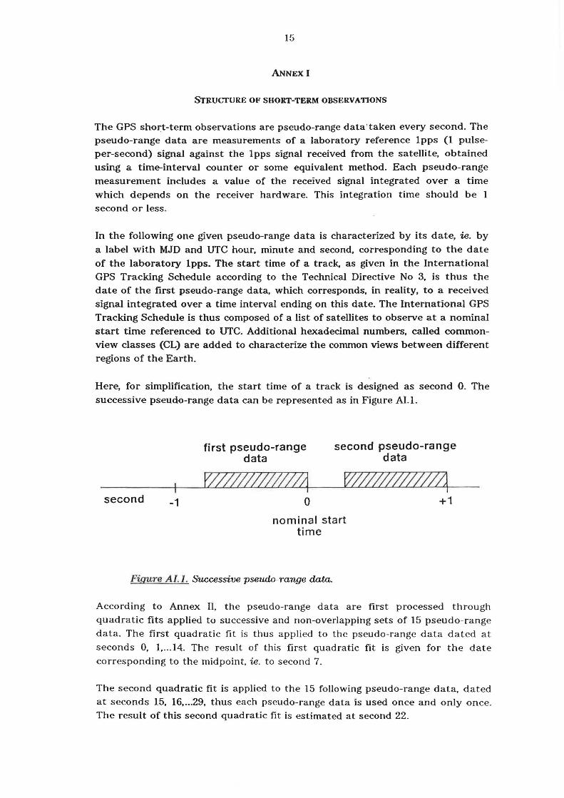
Here. for simplification. the start time of a track is designed as second O. The successive pseudo-range data can be represented as in Figure ALI.

second -1

first pseudo-range data

WllIII//IIIIL1 o

second pseudo-range data

[1"11/// ////// hl +1

nominal start time

Figure A l.I. Successive pseudo-range data.

According to Annex II. the pseudo-range data are first processed through quadratic fits applied to successive and non-overlapping sets of 15 pseudo-range data. The first quadratic fit is thus applied to the pseudo-range data dated at seconds O. 1 •... 14. The result of this first quadratic fit is given for the date

corresponding to the midpoint, ie. to second 7.

The second quadratic fit is applied to the 15 following pseudo-range data. dated at seconds 15. 16 •... 29. thus each pseudo-range data is used once and only once. The result of this second quadratic fit is estimated at second 22.

16

The first dates of quadratic fits are thus seconds 0 [mod 15], the last dates of quadratic fits are seconds 14 [mod 15] and the dates of quadratic fit results are

seconds 7 [modI5]. This can be represented as shown in Figure A1.2.

1st set 52nd set

111 111111 1111 111 1111 111111 III 11 111111 J 1111 1 J I l uu :J IIIIIIIIIIIII! 111 1 ,

second o 7 15 22 30 37 1 765

/// / 772 779

\ \ 52 results of quadratic fits

Figure AI.2. First dates of quadratic fits and dates of the results of quadratic fits.

According to Technical Directive No 2, each full track corresponds to the

recording of 780 pseudo-range data, which are dated from second 0 to second 779. The process thus uses 52 sets of 15 data and performs 52 quadratic fits,

whose results are dated at second 7, 22, ... 772. A linear fit is then applied to

these results (see Annex II).

Notes:

- From the above, it appears that the duratWn of a jull-length is equal to 779 s and 'lWt to 780 s, as is usuaUy said. ln fact, this is 'lWt true: as pseudo-range measurements are integrated over a time interval, the first begins before second 0 and the last ends at second 779. For simplification, the track length, appearing under the acronym TRKL, is taken to be 780 s for juU-length tracks, or to be the number of pseudo-range measurements for shorter tracks.

- Several linear fits are performed to jurther reduce the quadratic fit results. The results of these linear fits are then estimated at the date corresponding to the middle of the actual track (see Annex Ill). This particular date does 'lWt appear in the data file, as only the starting date is reported. Rigourously it should be labelled second 389,5 for jull-Length tracks and does 'lWt correspond ta an even second.

17

.rumExU

PROCESSING OF GPS SHORT-TERM DATA

TA.KEN OVER A FULL TRACK

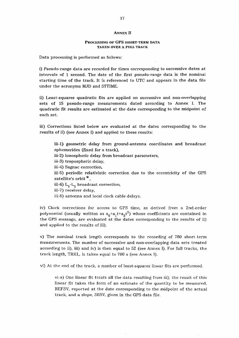
Data processing is performed as follows:

i) Pseudo-range data are recorded for times corresponding to successive dates at intervals of 1 second. The date of the first pseudo-range data is the nominal starting time of the track. It is referenced to UTC and appears in the data file under the acronyms MJD and STTIME.

ii) Least-squares quadratic fits are applied on successive and non-overlapping sets of 15 pseudo-range measurements dated according to Annex 1. The quadratic fit results are estimated at the date corresponding to the midpoint of each set.

iii) Corrections listed below are evaluated at the dates corresponding to the results of ii) (see Annex 1) and applied to these results:

iii-l) geometric delay from ground-antenna coordinates and broadcast

ephemerides (fixed for a track), iii-2) ionospheric delay from broadcast parameters, iii-3) tropospheric delay, iii-4) Sagnac correction, iii-5) periodic relativistic correction due to the eccentricity of the GPS

satellite's orbit * , iii-6) L

1-L

2 broadcast correction,

iii-7) receiver delay,

iii-8) antenna and local-dock cable delays.

iv) Clock corrections for access to GPS time, as derived from a 2nd-order polynomial (usually written as aO+a

l t+a

2t 2) whose coefficients are contained in

the GPS message, are evaluated at the dates corresponding to the results of ii) and applied to the results of iii).

v) The nominal track length corresponds to the recording of 780 short-term measurements. The number of successive and non-overlapping data sets treated according to ii), iii) and iv) is then equal to 52 (see Annex 1). For full tracks, the track length, TRKL, is taken equal to 780 s (see Annex 1).

vi) At the end of the track, a number of least-squares linear fits are performed.

vi-a) One linear fit treats aIl the data resulting from iii); the result of this linear fit takes the form of an estimate of the quantity to be measured,

REFSV, reported at the date corresponding to the midpoint of the actual track. and a slope, SRSV. given in the GPS data file.

18

vi-b) One linear fit treats all the data resulting from iv); the result of this linear fit takes the form of an estimate of the quantity to be measured, REFGPS, reported at the date corresponding to the midpoint of the actual track, a slope, SRGPS, and a rms, DSG, given in the GPS data file.

vi-c) One linear fit treats the modelled ionospheric corrections evaluated in iii-2); the result of this linear fit takes the form of an estimate of the

modelled ionospheric delay, MDIO, reported at the date corresponding to

the midpoint of the actual track, and a slope, SM DI, given in the GPS

data file.

vi-d) One linear fit treats the modelled tropospheric corrections

evaluated in iii-3); the result of this linear fit takes the form of an

estimate of the modelled tropospheric delay, MDTR, reported at the date

corresponding to the midpoint of the actual track, and a slope, SMDT, given in the GPS data file.

vi-e) One linear fit treats the measured ionospheric corrections obtained

from a Ionospheric Measurement System, if available, at the dates

corresponding to the results of ii); the result of this linear fit takes the form of an estimate of the measured ionospheric delay, MSIO, reported at

the date corresponding to the midpoint of the actual tracl<, a slope, SMSI,

and a rms, ISG, given in the GPS data file.

* The constant part of the relativistic correction to the frequency, consisting of

the gravitational red shift and the second order Doppler effect, is applied before launch to the satellite oscillators as a frequency offset.

Note:

TM Group on GPS Time Transfer Standards gives a tolerance for data

which is not in the form of pseudo-ranges at intervals of 1 second if the

hardware of the GPS time receiver currently in operation does not generate such data.

For existing receivers which takes short-term observations every 0,6

second, the data processing could copy closely the one given in this Annex, with quadratic fits over durations of about 15 s followed by a linear fit.

For existing receivers which takes short-term observations every 6 seconds,

it seems reasonable to process directly 6-second data through a linear fit.

ft is expected that new receivers will operate in accordance with the basic

1 second pseudo-range data.

19

ANNEXm

GGTfS GPS DATA FORMAT VERSION 01

The GGTTS GPS Data Format Version 01 comprises:

i) a file header with detaHed information on the GPS equipment (line 1 to 16).

ii) a blank line (line 17).

iii) a line header with the acronyms of the reported quantities Oine 18).

iv) a unit header with the units used for the reported quantities Oine 19).

v) a series of data lin es Oine 20. 21. 22 •...• (n-1). n, ... etc.). one line corresponding to one GPS track. The GPS tracks are ordered in chronological order. the track reported in line n occuring after the track reported in line (n-1).

Each line of the data file is limited to 128 columns and is terrninated by a carriage-return and a line feed.

Notes:

- A * stands for a space, ASCII value 20 (hexadecimal) . Text to be written in the data file is indicated by 1

- The line order described in v) does not correspond to the line order output by 11Wst receivers at present time.

20

1. File header

Line 1: 'GGTTS*GPS*DATA*FORMAT*VERSION*=*' N Title to be written. N = 01. 34 columns (as long as N < 100) .

Line 2: 'REV*DATE*=*' YYYY' - , MM' - , DD Revision date of the header data, changed when 1 parameter given in the header is changed. YYYY-MM-DD for year, month and day.

21 columns.

Line3: 'RCVR*=*' MAKER'*'TYPE'*'SERIAL NUMBER'*'YEAR'*' SOFTWARE NUMBER

Maker acronym, type, seriai number, first year of

operation, and eventually software number of the GPS

time receiver.

As many columns as necessary.

Line4: 'CH*=*' CHANNEL NUMBER Number of the channel used to produce the data

included in the file,

CH = 01 for a one-channel receiver.

7 columns (as long as CH < 100).

Line5: 'IMS*=*' MAKER'*'TYPE'*'SERIAL NUMBER'*'YEAR'*' SOFTWARE NUMBER

Maker acronym, type, seriai number, first year of

operation, and eventually software number of the Ionospheric Measurement System.

IMS = 99999 if none. Similar to Une 3 if included in the time receiver.


Line 6: 'LAB*=*' LABORATORY Acronym of the laboratory where observations are performed .


21

Line 7: 'X*=*' X COORDINATE '*m' X coordinate of the GPS antenna, in m and given with at least 2 decimals. As many columns as necessary.

Line 8: 'Y*=*' y COORDINATE '*m' y coordinate of the GPS antenna, in m and given with at least 2 decimals. As many columns as necessary.

Line 9: 'Z*=*' Z COORDINATE '*m' Z coordinate of the GPS antenna, in m and given with at least 2 decimals. As many columns as necessary.

LinelO: 'FRAME*=*' FRAME Designation of the reference frame of the GPS antenna

coordinates.


Linell: 'COMMENTS*=*' COMMENTS Any comments about the coordinates, for example the

method of determination or the estimated uncertainty. As many columns as necessary.

Line 12: 'INT*DLY*=*' INTERNAL DELAY '*ns' InternaI delay entered in the GPS time receiver, in ns

and given with 1 decimal. As many columns as necessary.

Une 13: 'CAB*DLY*=*' CABLE DELAY '*ns' Delay coming from the cable length from the GPS antenna to the main unit, entered in the CPS time

receiver, in ns and given with 1 decimal. As many columns as necessary.

Line 14: 'REF*DLY*=*' REFERENCE DELAY '*ns' Delay coming from the cable length from the reference output to the main unit, entered in the GPS time receiver, in ns and given with 1 decimal. As many columns as necessary.

22

Linel5: 'REF*=*' REFERENCE

Line 16: 'CKSUM*=*' XX

Line 17: blank line.

Identifier of the time reference entered in the GPS time receiver. For laboratories contributing to TAI it can be the 7-digit code of a dock or the 5-digit code of a local UTC, as attributed by the BIPM. As many columns as necessary.

Header check-sum: hexadecimal representation of the

sum, modulo 256, of the ASCII values of the characters which constitute the complete header, beginning with the first letter 'G' of 'GGTTS' in Line l, induding ail spaces indicated as * and corresponding to the ASCII value 20 (hexadecimal), ending with the space after '='

of Line 16 just preceding the actual check sum value, and excluding aU carriage returns or line feeds. 10 columns.

23

2. Line header

2 .1. No measured ionosphe ric delays ava ila ble

Line 5 of the header indicates: IMS = 99999

No ionospheric measurements are available, the specifie format of the line header is

as follows:

Line 18.1: 1 PRN*CL**MJD**STTIME*TRKL*ELV*AZTH***REFSV***** *SRSV*****REFGPS****SRGPS**DSG*IOE*MDTR*SMDT*MDIO*SMDI*CK'

Line to be written. The acronyms are explained in 4.

103 columns.

2.2. Measured ionosphe ric d elays a va ilab le

Line 5 of the header indicates, for instance:

IMS = AIR NIMS 003 1992 (Example with fictitious data of Section 6.)

Ionospheric measurements are avaiIable, the specifie format of the line header is as follows:

Line 18.2: 1 PRN*CL**MJD**STTIME*TRKL*ELV*AZTH***REFSV***** *SRSV*****REFGPS****SRGPS**DSG*IOE*MDTR*SMDT*MDIO*SMDI* MSIO*SMSI*ISG*CK'

Line to be written.

The acronyms are explained in 4 .

117 columns.

24

3. Unit header

3.1. No measured ionospheric delays available

Line 19.1: '*************hhmmss**s** .1dg* .1dg**** .1ns***** .1psjs*****.lns****.lpsjs*.lns*****.lns.lpsjs.lns.lpsjs**'

Line to be written 103 columns.

3.2. Measured ionospheric delays available

Line 19.2: '*************hhmmss**s** .1dg* .1dg**** .1ns***** .1ps/s*****.lns****.lps/s*.lns*****.lns.lps/s.lns.lpsls .1ns.lpsjs.lns**'

Line to be written

117 columns.

25

4. Data line

Line 20, column 1: space, ASCII value 20 (hexadecimal).

Une 20, columns 2-3: '12' PRN Satellite vehicle PRN number.

No unit.

Line 20, column 4: space, ASCII value 20 (hexadecimal) .

Line 20, columns 5-6: '12' CL Common-view hexadecimal class byte.

No unit.

Une 20, column 7: space, ASCII value 20 (hexadecimal).

Une 20, columns 8-12: '12345' MJD

Modified Julian Day.

No unit.

Une 20, column 13: space, ASCII value 20 (hexadecimal) .

Une 20, columns 14-19: '121212' STTIME Date of the start time of the track (see Annex 1).

In hour, minute and second referenced to UTC.


Line 20, columns 21-24: '1234' TRKL

Track length, 780 for full tracks (see Annex 1).

In s.

Une 20, column 25: space, ASCII value 20 (hexadecimal) .

Line 20, columns 26-28: '123' ELV

Satellite elevation at the date corresponding to the

midpoint of the track.

In 0.1 degree.

Une 20, column 29 : space. ASCII value 20 (hexadecimal) .

Une 20, columns 30-33: '1234' AZTH

Satellite azimuth at the date corresponding to the midpoint of the track.

In 0.1 degree.


26

Line 20, columns 35-45: 1 +1234567890 1 REFSV Time difference resulting from the treatment vi-a) of

Annex II. In 0.1 ns.


Line 20, columns 47-52: 1 +12345 1 SRSV Slope resulting from the treatment vi-a) of Annex II.

In 0.1 ps/s.


Line 20, columns 54-64: 1 +1234567890 1 REFGPS

Time difference resulting from the treatment vi-b) of

Annex II. In 0.1 ns.


Line 20, columns 66-71: 1 +12345 1 SRGPS

Slope resulting from the treatment vi-b) of Annex II.

In 0.1 ps/s.


Line 20, columns 73-76: 11234 1 DSG

[Data Sigma] Root mean square of the residuals to the

linear fit vi-b) of Annex II.

In 0.1 ns.


Line 20, columns 78-80: 1123' IOE

[Index of Ephemeris 1 Three digit decimal code (0-255)

indicating the ephemeris used for the computation. No unit.


Line 20, columns 82-85: '1234' MDTR

Modelled tropospheric delay resulting from the linear fit

vi-d) of Annex II.

In 0.1 ns.


27

Une 20, columns 87-90: '+123' SMOT Siope of the modelled tropospheric delay resulting from

the linear fit vi-d) of Annex Il.

In 0.1 ps/s.


Une 20. columns 92-95: '1234' MOIO Modelled ionospheric delay resulting from the linear fit

vi-c) of Annex Il. In 0.1 ns.

Une 20. column 96: space. ASCII value 20 (hexadecimal) .

Une 20. columns 97-100: '+123' SMOI Slope of the modelled ionospheric delay resulting from

the linear fit vi-c) of Annex II.

In 0.1 ps/s.

Une 20. column 101: space. ASCII value 20 (hexadecimal) .

4.1. No measured ionos phe ric d e la ys ava ila bl e

Une 20.1. columns 102-103: '12' CK Data Une check-sum: hexadecimal representation of the

sum. modulo 256. of the ASCII values of the characters

which constitute the data line, from column 1 to column

101 (both included).

Une 20.1. columns 104-128: '1234567890123456789012345'

Optional comments on the data line, constituted of

characters which are not included in the line check-sum

CK.

4 .2. Measured ionos phe r ic delays availa ble

Une 20.2, columns 102-105: 11234 1 MSIO

Measured ionospheric delay resulting from the linear fit

vi-e) of Annex II.

In 0.1 ns .

Une 20.2. column 106: space, ASCII value 20 (hexadecimal) .

Une 20.2, columns 107-110: '+123' SMSI

Slope of the measured ionospheric delay resulting from

the linear fit vi-e) of Annex II. ln 0.1 ps/s.

28

Une 20.2, column Ill: space, ASCII value 20 (hexadecimal).

Une 20.2, columns 112-114: '123' ISG [Ionospheric Sigma] Root mean square of the residuals to the linear fit vi-e) of Annex II.

In 0.1 ns.

Une 20.2, column 115: space, ASCII value 20 (hexadecimal) .

Une 20.2, columns 116-117: '12' CK Data line check-sum: hexadecimal representation of the

sum, modulo 256, of the ASCII values of the characters

which constitute the data line, from column 1 to column 115 (both included).

Une 20.2, columns 118-128: '12345678901'

Notes:

Optional comments on the data line, constituted of characters which are not included in the line check

sumo

- Any missing data slwuld be replaœd by series of 9.

- When the number of columns reserved for reporting a quantity is too large, the value of the corresponding quantity must be preceded by spaces, ASCII value 20 in hexadecimal (see Section 6 of Annex III).

5. Conclusions

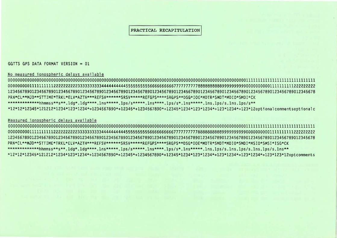
The format for one data line can be represented as follows:

5.1. No meas ur ed iono~ p h e ri c de l ays av a i l ab le

00000000000000000000000000000000000000000000000000000000000000000000000000000000000000000000000000011111111111111111111111111111 000000000111111111122222222223333333333444444444455555555556666666666777777777788888888889999999999000000000 01111111111222222222 12345678901234567890123456789012345678901234567890123456789012345678901234567890123456789012345678901234567890123456789012345678 PRN*CL**MJD**STTIME*TRKL*ELV*AZTH***REFSV******SRSV*****REFGPS****SRGPS**DSG*IOE*MDTR*SMOT*MDIO*SMDI*CK *************hhmmss**s**.1dg*.1dg****.1ns*****.1ps/s*****.1ns****.1ps/s*.lns*****.lns.1ps/s.1ns.1ps/s** *12*12*12345*121212*1234*123*1234*+1234567890*+12345*+1234567890*+12345*1234*123*1234*+123*1234*+123*12optionalcommentsopt1onalc

5.2. Measur ed i onos pheri c delays available

N ~

00000000000000000000000000000000000000000000000000000000000000000000000000000000000000000000000000011111111111111111111111111111 00000000011111111112222222222333333333344444444445555555555666666666677777777778888888888999999999900000000001111111111222222222 1234567890123456789Ô123456789012345678901234567890123456789012345678901234567890123456789012345678901234567890123456789012345678 PRN*CL**MJO**STTIME*TR KL*ELV*AZTH***REFSV******SRSV*****REFGPS****SRGPS**OSG*IOE*MOTR*SMOT*MOIO*SMDI*MSIO*SMSI*ISG*CK *************hhmmss**s**.ldg*.ldg****.lns*****.1ps/s*****.1ns****.1ps/s*.1ns*****.1ns.1ps/s.1ns.1ps/s.1ns.1ps/s.1ns** *12*12*12345*121212*1234*123*1234*+1234567890*+12345*+1234567890*+12345*1234*123*1234*+123*1234*+123*1234*+123*123*12optcomments

6. Example (fictitious data)

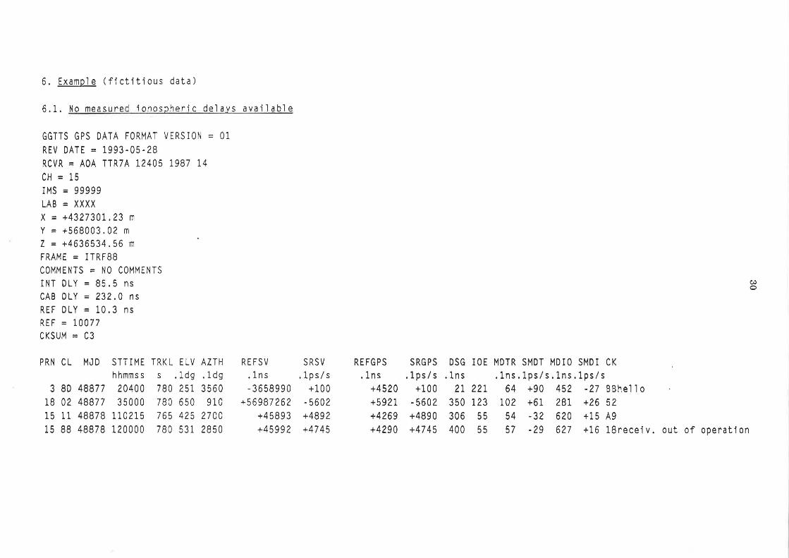
6.1. No measured ionospheric delays available

GGTTS GPS DATA FORMAT VERSION = 01 REV DATE = 1993-05-28 RCVR = AOA TTR7A 12405 1987 14 CH = 15 IMS = 99999 LAB = XXXX X = +4327301.23 m y = +568003.02 m Z = +4636534.56 m FRAME = ITRF88 COMMENTS = NO COMMENTS INT DLY = 85.5 ns CAB DLY = 232.0 ns REF DLY = 10.3 ns RH = 10077 CKSUM = C3

PRN CL MJO STTIME TRKL ELV AZTH hhmmss s .1dg .ldg

3 80 48877 20400 780 251 3560 18 02 48877 35000 780 650 910 15 Il 48878 110215 765 425 2700 15 88 48878 120000 780 531 2850

REFSV .lns -3658990

+56987262 +45893 +45992

SRSV REFGPS SRGPS .lps/s .lns .lps/s

+100 +4520 +100 -5602 +5921 -5602 +4892 +4269 +4890 +4745 +4290 +4745

DSG IOE MDTR SMDT MOrO SMDr CK .1ns .lns.lps/s.1ns.1ps/s

21 221 64 +90 452 -27 BBhello 350 123 102 +61 281 +26 52 306 55 54 -32 620 +15 A9 400 55 57 -29 627 +16 18receiv. out of operation

C,..) o

6.2. Mea sured i onospheric de l ays avaiJable

GGTTS GPS DATA FORMAT VERSION = 01 REV DATE = 1993-05-28 RCVR = AOA TTR7A 12405 1987 14 CH = 15 IMS = AIR NIMS 003 1992 LAB = XXXX X = +4327301.23 m y = +568003.02 m Z = +4636534.56 m FRAME = ITRF88 COMMENTS = NO COMMENTS INT DLY = 85.5 ns CAB OLY = 232.0 ns REF DLY = 10.3 ns REF = 10077 CKSUM = 49

PRN CL MJD STTIME TRKL ELV AZTH hhmmss 5 .1dg .1dg

3 8D 48877 20400 780 251 3560 18 02 48877 35000 780 650 910 15 11 48878 110215 765 425 2700 15 88 48878 120000 780 531 2850

REFSV .1ns -3658990

+56987262 +45893 +45992

SRSV .1ps/s

+100 -5602 +4892 +4745

~ -

REFGPS SRGPS DSG IDE MDTR SMDT MDIO SMDI MSIO SMSI ISG CK .1ns .1ps/s .1ns .lns.1ps/s.1ns.1ps/s.1ns.1p~/s.1ns

+4520 +100 21 221 64 +90 452 -27 480 -37 18 F4hell0 +5921 -5602 350 123 102 +61 281 +26 9999 9999 999 89no meas ion +4269 +4890 306 55 54 -32 620 +15 599 +16 33 29 +4290 +4745 400 55 57 -29 627 +16 601 +17 29 OOree out

1 ~M~TlCAL-REcAPITULATlo~J

GGTTS GPS DATA FORMAT VERSION = 01

No measured ionospheric delays available 00000000000000000000000000000000000000000000000000000000000000000000000000000000000000000000000000011111111111111111111111111111 00000000011111111112222222222333333333344444444445555555555666666666677777777778888888888999999999900000000001111111111222222222 12345678901234567890123456789012345678901234567890123456789012345678901234567890123456789012345678901234567890123456789012345678 PRN*CL**MJD**STTIME*TRKL*ELV*AZTH***REFSV******SRSV*****REFGPS****SRGPS**DSG*IOE*MDTR*SMDT*MDIO*SMDI*CK *************hhmmss**s**.1dg*.1dg****.1ns*****.1ps/s*****.1ns****.1ps/s*.1ns*****.1ns.1ps/s.1ns.1ps/s** *12*12*12345*121212*1234*123*1234*+1234567890*+12345*+1234567890*+12345*1234*123*1234*+123*1234*+123*12optionalcommentsoptionalc

Measured ionospheric delèys available 00000000000000000000000000000000000000000000000000000000000000000000000000000000000000000000000000011111111111111111111111111111 00000000011111111112222222222333333333344444444445555555555666666666677777777778888888888999999999900000000001111111111222222222 12345678901234567890123456789012345678901234567890123456789012345678901234567890123456789012345678901234567890123456789012345678 PRN*CL**MJD**STTIME*TRKL*ELV*AZTH***REFSV******SRSV*****REFGPS****SRGPS**DSG*IOE*MDTR*SMOT*MOIO*SMDI*MSIO*SMSI*ISG*CK *************hhmmss**s**.1dg*.1dg****.1ns*****.lps/s*****.1ns****.1ps/s*.1ns*****.1ns.1ps/s.1ns.1ps/s.1ns.1ps/s.1ns** *12*12*12345*121212*1234*123*1234*+1234567890*+12345*+1234567890*+12345*1234*123*1234*+123*1234*+123*1234*+123*123*12optcomments

Example (fietitious data) GGTTS GPS DATA FORMAT VERSION = 01 REV DATE = 1993-05-28 RCVR = AOA TTR7A 12405 1987 14 CH = 15 IMS = 99999 or IMS = AIR NIMS 003 1992 LAB = XXXX X = +4327301.23 m y = +568003.02 m Z = +4636534.56 m FRAME = ITRF88 COMMENTS = NO COMMENTS INT DLY = 85.5 ns CAB DLY = 232.0 ns REF DLY = 10.3 ns REF = 10077 CKSUM = C3 or CKSUM = 49

No measured ionospherie dela~s available PRN CL MJD STTIME TRKL ELV AZTH REFSV

hhmmss s .1dg .1dg .1ns 3 8D 48877 20400 780 251 3560 -3658990

18 02 48877 35000 780 650 910 +56987262 15 Il 48878 110215 765 425 2700 +45893 15 88 48878 120000 780 531 2850 +45992

Measured ionos pherie dela~s available PRN CL MJD STTIME TRKL ELV AZTH REFSV

hhmmss s .1dg .1dg .1ns 3 8D 48877 20400 780 251 3560 -3658990

18 02 48877 35000 780 650 910 +56987262 15 Il 48878 110215 765 425 2700 +45893 15 88 48878 120000 780 531 2850 +45992

SRSV .1ps/s

+100 -5602 +4892 +4745

SRSV .1ps/s

+100 -5602 +4892 +4745

REFGPS SRGPS DSG IOE MDTR SMDT MDIO SMDI CK .1ns .1ps/s .1ns .lns.1ps/s.1ns.1ps/s

+4520 +100 21 221 64 +90 452 -.27 BBhello +5921 -5602 350 123 102 +61 281 +26 52 +4269 +4890 306 55 54 -32 620 +15 A9 +4290 +4745 400 55 57 -29 627 +16 18reeeiv. out of operation

REFGPS SRGPS DSG IOE MDTR SMDT MDIO SMDI MSIO SMSI ISG CK .1ns .1ps/s .1ns .lns.1ps/s.1ns.1ps/s.1ns.1ps/s.1ns

+4520 +100 21 221 64 +90 452 -27 480 -37 18 F4hello +5921 -5602 350 123 102 +61 281 +26 9999 9999 999 89no meas ion +4269 +4890 306 55 54 -32 620 +15 599 +16 33 29 +4290 +4745 400 55 57 -29 627 +16 601 +17 29 OOree out

Documents

Rapport BIPM-1993/06: Technical directives for ... · complementary to the Subcommittee on Time of the Civil GPS Service Interface ... - the need for absolu te as weIl as relative