Random Variables, Distributions, and Expectations

ii

“WMMY-SmallBook-1” — 2011/10/27 — 9:12 — page 49 — #63 ii

ii

ii

Chapter 2

Random Variables, Distributions,and Expectations

2.1 Concept of a Random Variable

Statistics is concerned with making inferences about populations and populationcharacteristics. Experiments are conducted with results that are subject to chance.The testing of a number of electronic components is an example of a statisticalexperiment, a term that is used to describe any process by which several chanceobservations are generated. It is often important to allocate a numerical descriptionto the outcome. For example, the sample space giving a detailed description of eachpossible outcome when three electronic components are tested may be written

S = {NNN,NND,NDN,DNN,NDD,DND,DDN,DDD},

where N denotes nondefective and D denotes defective. One is naturally concernedwith the number of defectives that occur. Thus, each point in the sample space willbe assigned a numerical value of 0, 1, 2, or 3. These values are, of course, randomquantities determined by the outcome of the experiment. They may be viewed asvalues assumed by the random variable X , the number of defective items whenthree electronic components are tested.

Definition 2.1: A random variable is a variable that associates a real number with each elementin the sample space.

We shall use a capital letter, say X, to denote a random variable and its correspond-ing small letter, x in this case, for one of its values. In the electronic componenttesting illustration above, we notice that the random variable X assumes the value2 for all elements in the subset

E = {DDN,DND,NDD}

of the sample space S. That is, each possible value of X represents an event thatis a subset of the sample space for the given experiment.

49

ii


ii

ii

50 Chapter 2 Random Variables, Distributions, and Expectations

Example 2.1: Two balls are drawn in succession without replacement from an urn containing 4red balls and 3 black balls. The possible outcomes and the values y of the randomvariable Y , where Y is the number of red balls, are

Sample Space yRR 2RB 1BR 1BB 0

Example 2.2: A stockroom clerk returns three safety helmets at random to three steel millemployees who had previously checked them. If Smith, Jones, and Brown, in thatorder, receive one of the three hats, list the sample space for the possible ordersof returning the helmets, and find the value m of the random variable M thatrepresents the number of correct matches.

Solution : If S, J , and B stand for Smith’s, Jones’s, and Brown’s helmets, respectively, thenthe possible arrangements in which the helmets may be returned and the numberof correct matches are

Sample Space mSJB 3SBJ 1BJS 1JSB 1JBS 0BSJ 0

In each of the two preceding examples, the sample space contains a finite numberof elements. On the other hand, when a die is thrown until a 5 occurs, we obtaina sample space with an unending sequence of elements,

S = {F,NF,NNF,NNNF, . . . },

where F and N represent, respectively, the occurrence and nonoccurrence of a 5.But even in this experiment, the number of elements can be equated to the numberof whole numbers so that there is a first element, a second element, a third element,and so on, and in this sense can be counted.

Definition 2.2: If a sample space contains a finite number of possibilities or an unending sequencewith as many elements as there are whole numbers, it is called a discrete samplespace.

When the random variable is categorical in nature, it is often called a dummyvariable. A good illustration is the case in which the random variable is binary innature, as shown in the following example.

Example 2.3: Consider the simple experiment in which components are arriving from the pro-duction line and they are stipulated to be defective or not defective. Define the

ii


ii

ii

2.1 Concept of a Random Variable 51

random variable X by

X =

{1, if the component is defective,

0, if the component is not defective.

Clearly the assignment of 1 or 0 is arbitrary though quite convenient. This willbecome clear in later chapters. The random variable for which 0 and 1 are chosento describe the two possible values is called a Bernoulli random variable.

Further illustrations of random variables appear in the following examples.

Example 2.4: Statisticians use sampling plans to either accept or reject batches or lots ofmaterial. Suppose one of these sampling plans involves sampling independently 10items from a lot of 100 items in which 12 are defective.

Let X be the random variable defined as the number of items found defec-tive in the sample of 10. In this case, the random variable takes on the values0, 1, 2, . . . , 9, 10.

Example 2.5: Suppose a sampling plan involves sampling items from a process until a defectiveis observed. The evaluation of the process will depend on how many consecutivenondefective items are observed. In that regard, letX be a random variable definedby the number of items observed before a defective is found. With N a nondefectiveand D a defective, the outcomes in the sample space are D given X = 1, ND givenX = 2, NND given X = 3, and so on.

Example 2.6: Interest centers around the proportion of people who respond to a certain mailorder solicitation. Let X be that proportion. X is a random variable that takeson all values x for which 0 ≤ x ≤ 1.

Example 2.7: Let X be the random variable defined by the waiting time, in hours, betweensuccessive speeders spotted by a radar unit. The random variable X takes on allvalues x for which x ≥ 0.

The outcomes of some statistical experiments may be neither finite nor count-able. Such is the case, for example, when one conducts an investigation measuringthe distances that a certain make of automobile will travel over a prescribed testcourse on 5 liters of gasoline. Assuming distance to be a variable measured to anydegree of accuracy, then clearly we have an infinite number of possible distancesin the sample space that cannot be equated to the number of whole numbers. Or,if one were to record the length of time for a chemical reaction to take place, onceagain the possible time intervals making up our sample space would be infinite innumber and uncountable. We see now that all sample spaces need not be discrete.

Definition 2.3: If a sample space contains an infinite number of possibilities equal to the numberof points on a line segment, it is called a continuous sample space.

A random variable is called a discrete random variable if its set of possibleoutcomes is countable. The random variables in Examples 2.1 to 2.5 are discreterandom variables. But a random variable whose set of possible values is an entire

ii


ii

ii


interval of real numbers is not discrete. When a random variable can take onvalues on a continuous scale, it is called a continuous random variable. Oftenthe possible values of a continuous random variable are precisely the same valuesthat are contained in the continuous sample space. Obviously, the random variablesdescribed in Examples 2.6 and 2.7 are continuous random variables.

In most practical problems, continuous random variables represent measureddata, such as all possible heights, weights, temperatures, distances, or life periods,whereas discrete random variables represent count data, such as the number ofdefectives in a sample of k items or the number of highway fatalities per year ina given state. Note that the random variables Y and M of Examples 2.1 and 2.2both represent count data, Y the number of red balls and M the number of correcthat matches.

2.2 Discrete Probability Distributions

A discrete random variable assumes each of its values with a certain probability.In the case of tossing a coin three times, the variable X, representing the numberof heads, assumes the value 2 with probability 3/8, since 3 of the 8 equally likelysample points result in two heads and one tail. If one assumes equal weights for thesimple events in Example 2.2, the probability that no employee gets back the righthelmet, that is, the probability that M assumes the value 0, is 1/3. The possiblevalues m of M and their probabilities are

m 0 1 3

P(M = m) 13

12

16

Note that the values of m exhaust all possible cases and hence the probabilitiesadd to 1.

Frequently, it is convenient to represent all the probabilities of the values of arandom variable X by a formula. Such a formula would necessarily be a functionof the numerical values x that we shall denote by f(x), g(x), r(x), and so forth.Therefore, we write f(x) = P (X = x); that is, f(3) = P (X = 3). The set ofordered pairs (x, f(x)) is called the probability mass function, probabilityfunction, or probability distribution of the discrete random variable X.

Definition 2.4: The set of ordered pairs (x, f(x)) is a probability mass function, probabilityfunction, or probability distribution of the discrete random variable X if, foreach possible outcome x,

1. f(x) ≥ 0,

2.∑xf(x) = 1,

3. P (X = x) = f(x).

Example 2.8: A shipment of 20 similar laptop computers to a retail outlet contains 3 that aredefective. If a school makes a random purchase of 2 of these computers, find theprobability distribution for the number of defectives.

ii


ii

ii

2.2 Discrete Probability Distributions 53

Solution : Let X be a random variable whose values x are the possible numbers of defectivecomputers purchased by the school. Then x can only take the numbers 0, 1, and2. Now

f(0) = P (X = 0) =

(30

)(172

)(202

) =68

95, f(1) = P (X = 1) =

(31

)(171

)(202

) =51

190,

f(2) = P (X = 2) =

(32

)(170

)(202

) =3

190.

Thus, the probability distribution of X isx 0 1 2

f(x) 6895

51190

3190

Example 2.9: If a car agency sells 50% of its inventory of a certain foreign car equipped withside airbags, find a formula for the probability distribution of the number of carswith side airbags among the next 4 cars sold by the agency.

Solution : Since the probability of selling an automobile with side airbags is 0.5, the 24 = 16points in the sample space are equally likely to occur. Therefore, the denominatorfor all probabilities, and also for our function, is 16. To obtain the number ofways of selling 3 cars with side airbags, we need to consider the number of waysof partitioning 4 outcomes into two cells, with 3 cars with side airbags assignedto one cell and the model without side airbags assigned to the other. This can bedone in

(43

)= 4 ways. In general, the event of selling x models with side airbags

and 4− x models without side airbags can occur in(4x

)ways, where x can be 0, 1,

2, 3, or 4. Thus, the probability distribution f(x) = P (X = x) is

f(x) =1

16

(4

x

), for x = 0, 1, 2, 3, 4.

There are many problems where we may wish to compute the probability thatthe observed value of a random variable X will be less than or equal to some realnumber x. Writing F (x) = P (X ≤ x) for every real number x, we define F (x) tobe the cumulative distribution function of the random variable X.

Definition 2.5: The cumulative distribution function F (x) of a discrete random variable Xwith probability distribution f(x) is

F (x) = P (X ≤ x) =∑t≤x

f(t), for −∞ < x < ∞.

For the random variable M , the number of correct matches in Example 2.2, wehave

F (2) = P (M ≤ 2) = f(0) + f(1) =1

3+

1

2=

5

6.

The cumulative distribution function of M is

F (m) =

0, for m < 0,13 , for 0 ≤ m < 1,56 , for 1 ≤ m < 3,

1, for m ≥ 3.

ii


ii

ii


One should pay particular notice to the fact that the cumulative distribution func-tion is a monotone nondecreasing function defined not only for the values assumedby the given random variable but for all real numbers.

Example 2.10: Find the cumulative distribution function of the random variable X in Example2.9. Using F (x), verify that f(2) = 3/8.

Solution : Direct calculations of the probability distribution of Example 2.9 give f(0)= 1/16,f(1) = 1/4, f(2)= 3/8, f(3)= 1/4, and f(4)= 1/16. Therefore,

F (0) = f(0) =1

16,

F (1) = f(0) + f(1) =5

16,

F (2) = f(0) + f(1) + f(2) =11

16,

F (3) = f(0) + f(1) + f(2) + f(3) =15

16,

F (4) = f(0) + f(1) + f(2) + f(3) + f(4) = 1.

Hence,

F (x) =

0, for x < 0,116 , for 0 ≤ x < 1,516 , for 1 ≤ x < 2,1116 , for 2 ≤ x < 3,1516 , for 3 ≤ x < 4,

1 for x ≥ 4.

Now

f(2) = F (2)− F (1) =11

16− 5

16=

3

8.

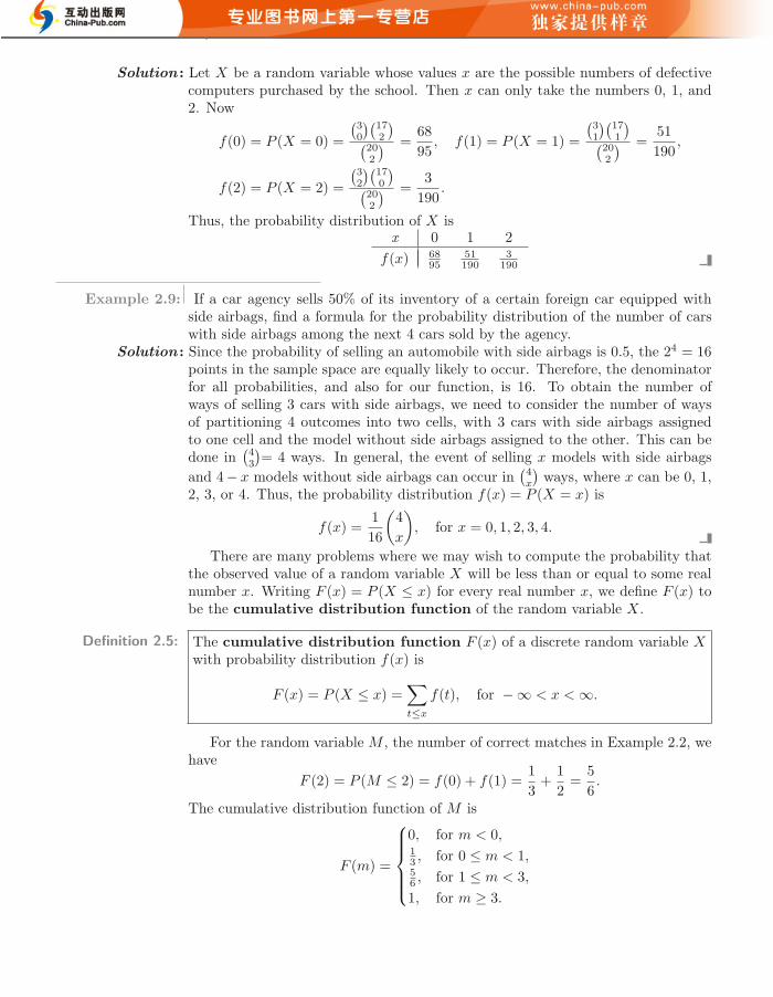
It is often helpful to look at a probability distribution in graphic form. Onemight plot the points (x, f(x)) of Example 2.9 to obtain Figure 2.1. By joiningthe points to the x axis either with a dashed or with a solid line, we obtain aprobability mass function plot. Figure 2.1 makes it easy to see what values of Xare most likely to occur, and it also indicates a perfectly symmetric situation inthis case.

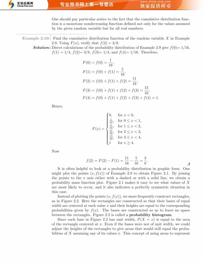
Instead of plotting the points (x, f(x)), we more frequently construct rectangles,as in Figure 2.2. Here the rectangles are constructed so that their bases of equalwidth are centered at each value x and their heights are equal to the correspondingprobabilities given by f(x). The bases are constructed so as to leave no spacebetween the rectangles. Figure 2.2 is called a probability histogram.

Since each base in Figure 2.2 has unit width, P (X = x) is equal to the areaof the rectangle centered at x. Even if the bases were not of unit width, we couldadjust the heights of the rectangles to give areas that would still equal the proba-bilities of X assuming any of its values x. This concept of using areas to represent

ii


ii

ii

2.3 Continuous Probability Distributions 55

x

f (x )

0 1 2 3 4

1/16

2/16

3/16

4/16

5/16

6/16

Figure 2.1: Probability mass function plot.

0 1 2 3 4x

f (x )

1/16

2/16

3/16

4/16

5/16

6/16

Figure 2.2: Probability histogram.

probabilities is necessary for our consideration of the probability distribution of acontinuous random variable.

The graph of the cumulative distribution function of Example 2.10, which ap-pears as a step function in Figure 2.3, is obtained by plotting the points (x, F (x)).

Certain probability distributions are applicable to more than one physical situa-tion. The probability distribution of Example 2.10, for example, also applies to therandom variable Y , where Y is the number of heads when a coin is tossed 4 times,or to the random variable W , where W is the number of red cards that occur when4 cards are drawn at random from a deck in succession with each card replaced andthe deck shuffled before the next drawing. Special discrete distributions that canbe applied to many different experimental situations will be considered in Chapter3.

F(x)

x

1/4

1/2

3/4

1

0 1 2 3 4

Figure 2.3: Discrete cumulative distribution function.

2.3 Continuous Probability Distributions

A continuous random variable has a probability of 0 of assuming exactly any of itsvalues. Consequently, its probability distribution cannot be given in tabular form.

ii


ii

ii


At first this may seem startling, but it becomes more plausible when we consider aparticular example. Let us discuss a random variable whose values are the heightsof all people over 21 years of age. Between any two values, say 163.5 and 164.5centimeters, or even 163.99 and 164.01 centimeters, there are an infinite numberof heights, one of which is 164 centimeters. The probability of selecting a personat random who is exactly 164 centimeters tall and not one of the infinitely largeset of heights so close to 164 centimeters that you cannot humanly measure thedifference is remote, and thus we assign a probability of 0 to the event. This is notthe case, however, if we talk about the probability of selecting a person who is atleast 163 centimeters but not more than 165 centimeters tall. Now we are dealingwith an interval rather than a point value of our random variable.

We shall concern ourselves with computing probabilities for various intervals ofcontinuous random variables such as P (a < X < b), P (W ≥ c), and so forth. Notethat when X is continuous,

P (a < X ≤ b) = P (a < X < b) + P (X = b) = P (a < X < b).

That is, it does not matter whether we include an endpoint of the interval or not.This is not true, though, when X is discrete.

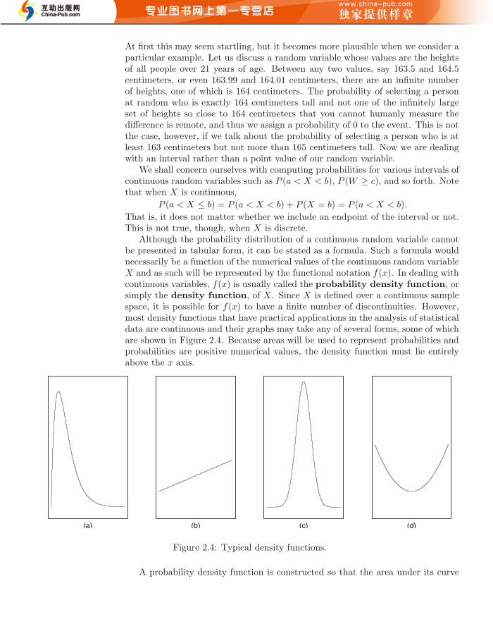
Although the probability distribution of a continuous random variable cannotbe presented in tabular form, it can be stated as a formula. Such a formula wouldnecessarily be a function of the numerical values of the continuous random variableX and as such will be represented by the functional notation f(x). In dealing withcontinuous variables, f(x) is usually called the probability density function, orsimply the density function, of X. Since X is defined over a continuous samplespace, it is possible for f(x) to have a finite number of discontinuities. However,most density functions that have practical applications in the analysis of statisticaldata are continuous and their graphs may take any of several forms, some of whichare shown in Figure 2.4. Because areas will be used to represent probabilities andprobabilities are positive numerical values, the density function must lie entirelyabove the x axis.

(a) (b) (c) (d)

Figure 2.4: Typical density functions.

A probability density function is constructed so that the area under its curve

ii


ii

ii

2.3 Continuous Probability Distributions 57

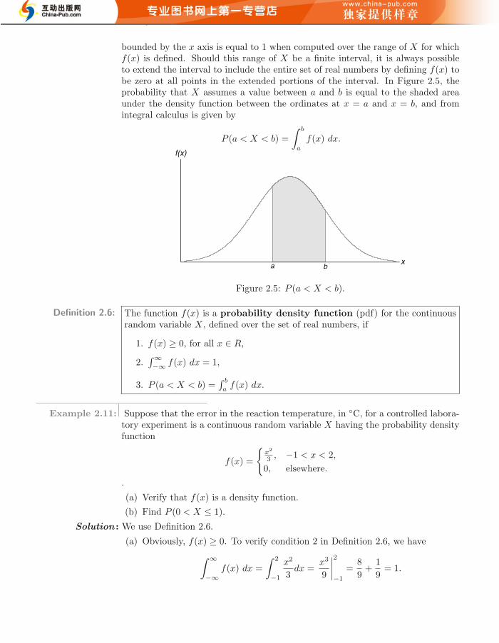
bounded by the x axis is equal to 1 when computed over the range of X for whichf(x) is defined. Should this range of X be a finite interval, it is always possibleto extend the interval to include the entire set of real numbers by defining f(x) tobe zero at all points in the extended portions of the interval. In Figure 2.5, theprobability that X assumes a value between a and b is equal to the shaded areaunder the density function between the ordinates at x = a and x = b, and fromintegral calculus is given by

P (a < X < b) =

∫ b

a

f(x) dx.

a bx

f(x)

Figure 2.5: P (a < X < b).

Definition 2.6: The function f(x) is a probability density function (pdf) for the continuousrandom variable X, defined over the set of real numbers, if

1. f(x) ≥ 0, for all x ∈ R,

2.∫∞−∞ f(x) dx = 1,

3. P (a < X < b) =∫ b

af(x) dx.

Example 2.11: Suppose that the error in the reaction temperature, in ◦C, for a controlled labora-tory experiment is a continuous random variable X having the probability densityfunction

f(x) =

{x2

3 , −1 < x < 2,

0, elsewhere.

.

(a) Verify that f(x) is a density function.

(b) Find P (0 < X ≤ 1).

Solution : We use Definition 2.6.

(a) Obviously, f(x) ≥ 0. To verify condition 2 in Definition 2.6, we have∫ ∞

−∞f(x) dx =

∫ 2

−1

x2

3dx =

x3

9

∣∣∣∣2−1

=8

9+

1

9= 1.

ii


ii

ii


(b) Using formula 3 in Definition 2.6, we obtain

P (0 < X ≤ 1) =

∫ 1

0

x2

3dx =

x3

9

∣∣∣∣10

=1

9.

Definition 2.7: The cumulative distribution function F (x) of a continuous random variableX with density function f(x) is

F (x) = P (X ≤ x) =

∫ x

−∞f(t) dt, for −∞ < x < ∞.

As an immediate consequence of Definition 2.7, one can write the two results

P (a < X < b) = F (b)− F (a)

and

f(x) =dF (x)

dx,

if the derivative exists.

Example 2.12: For the density function of Example 2.11, find F (x), and use it to evaluateP (0 < X ≤ 1).

Solution : For −1 < x < 2,

F (x) =

∫ x

−∞f(t) dt =

∫ x

−1

t2

3dt =

t3

9

∣∣∣∣x−1

=x3 + 1

9.

Therefore,

F (x) =

0, x < −1,x3+1

9 , −1 ≤ x < 2,

1, x ≥ 2.

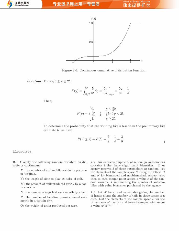
The cumulative distribution function F (x) is expressed in Figure 2.6. Now

P (0 < X ≤ 1) = F (1)− F (0) =2

9− 1

9=

1

9,

which agrees with the result obtained by using the density function in Example2.11.

Example 2.13: The Department of Energy (DOE) puts projects out on bid and generally estimateswhat a reasonable bid should be. Call the estimate b. The DOE has determinedthat the density function of the winning (low) bid is

f(y) =

{58b ,

25b ≤ y ≤ 2b,

0, elsewhere.

Find F (y) and use it to determine the probability that the winning bid is less thanthe DOE’s preliminary estimate b.

ii


ii

ii

Exercises 59

f (x )

x0 221 1

0.5

1.0

Figure 2.6: Continuous cumulative distribution function.

Solution : For 2b/5 ≤ y ≤ 2b,

F (y) =

∫ y

2b/5

5

8bdy =

5t

8b

∣∣∣∣y2b/5

=5y

8b− 1

4.

Thus,

F (y) =

0, y < 2

5b,5y8b − 1

4 ,25b ≤ y < 2b,

1, y ≥ 2b.

To determine the probability that the winning bid is less than the preliminary bidestimate b, we have

P (Y ≤ b) = F (b) =5

8− 1

4=

3

8.

Exercises

2.1 Classify the following random variables as dis-crete or continuous:

X: the number of automobile accidents per yearin Virginia.

Y : the length of time to play 18 holes of golf.

M : the amount of milk produced yearly by a par-ticular cow.

N : the number of eggs laid each month by a hen.

P : the number of building permits issued eachmonth in a certain city.

Q: the weight of grain produced per acre.

2.2 An overseas shipment of 5 foreign automobilescontains 2 that have slight paint blemishes. If anagency receives 3 of these automobiles at random, listthe elements of the sample space S, using the letters Band N for blemished and nonblemished, respectively;then to each sample point assign a value x of the ran-dom variable X representing the number of automo-biles with paint blemishes purchased by the agency.

2.3 Let W be a random variable giving the numberof heads minus the number of tails in three tosses of acoin. List the elements of the sample space S for thethree tosses of the coin and to each sample point assigna value w of W .

ii


ii

ii


2.4 A coin is flipped until 3 heads in succession oc-cur. List only those elements of the sample space thatrequire 6 or less tosses. Is this a discrete sample space?Explain.

2.5 Determine the value c so that each of the follow-ing functions can serve as a probability distribution ofthe discrete random variable X:

(a) f(x) = c(x2 + 4), for x = 0, 1, 2, 3;

(b) f(x) = c(2x

)(3

3−x

), for x = 0, 1, 2.

2.6 The shelf life, in days, for bottles of a certainprescribed medicine is a random variable having thedensity function

f(x) =

{20,000

(x+100)3, x > 0,

0, elsewhere.

Find the probability that a bottle of this medicine willhave a shell life of

(a) at least 200 days;

(b) anywhere from 80 to 120 days.

2.7 The total number of hours, measured in units of100 hours, that a family runs a vacuum cleaner over aperiod of one year is a continuous random variable Xthat has the density function

f(x) =

x, 0 < x < 1,

2− x, 1 ≤ x < 2,

0, elsewhere.

Find the probability that over a period of one year, afamily runs their vacuum cleaner

(a) less than 120 hours;

(b) between 50 and 100 hours.

2.8 The proportion of people who respond to a certainmail-order solicitation is a continuous random variableX that has the density function

f(x) =

{2(x+2)

5, 0 < x < 1,

0, elsewhere.

(a) Show that P (0 < X < 1) = 1.

(b) Find the probability that more than 1/4 but fewerthan 1/2 of the people contacted will respond tothis type of solicitation.

2.9 A shipment of 7 television sets contains 2 defec-tive sets. A hotel makes a random purchase of 3 of thesets. If x is the number of defective sets purchased bythe hotel, find the probability distribution of X. Ex-press the results graphically as a probability histogram.

2.10 An investment firm offers its customers munici-pal bonds that mature after varying numbers of years.Given that the cumulative distribution function of T ,the number of years to maturity for a randomly se-lected bond, is

F (t) =

0, t < 1,14, 1 ≤ t < 3,

12, 3 ≤ t < 5,

34, 5 ≤ t < 7,

1, t ≥ 7,

find

(a) P (T = 5);

(b) P (T > 3);

(c) P (1.4 < T < 6);

(d) P (T ≤ 5 | T ≥ 2).

2.11 The probability distribution of X, the numberof imperfections per 10 meters of a synthetic fabric incontinuous rolls of uniform width, is given by

x 0 1 2 3 4f(x) 0.41 0.37 0.16 0.05 0.01

Construct the cumulative distribution function of X.

2.12 The waiting time, in hours, between successivespeeders spotted by a radar unit is a continuous ran-dom variable with cumulative distribution function

F (x) =

{0, x < 0,

1− e−8x, x ≥ 0.

Find the probability of waiting less than 12 minutesbetween successive speeders

(a) using the cumulative distribution function of X;

(b) using the probability density function of X.

2.13 Find the cumulative distribution function of therandom variable X representing the number of defec-tives in Exercise 2.9. Then using F (x), find

(a) P (X = 1);

(b) P (0 < X ≤ 2).

2.14 Construct a graph of the cumulative distributionfunction of Exercise 2.13.

2.15 Consider the density function

f(x) =

{k√x, 0 < x < 1,

0, elsewhere.

(a) Evaluate k.

(b) Find F (x) and use it to evaluate

P (0.3 < X < 0.6).

ii


ii

ii

Exercises 61

2.16 Three cards are drawn in succession from a deckwithout replacement. Find the probability distributionfor the number of spades.

2.17 From a box containing 4 dimes and 2 nickels,3 coins are selected at random without replacement.Find the probability distribution for the total T of the3 coins. Express the probability distribution graphi-cally as a probability histogram.

2.18 Find the probability distribution for the numberof jazz CDs when 4 CDs are selected at random froma collection consisting of 5 jazz CDs, 2 classical CDs,and 3 rock CDs. Express your results by means of aformula.

2.19 The time to failure in hours of an importantpiece of electronic equipment used in a manufacturedDVD player has the density function

f(x) =

{1

2000exp(−x/2000), x ≥ 0,

0, x < 0.

(a) Find F (x).

(b) Determine the probability that the component (andthus the DVD player) lasts more than 1000 hoursbefore the component needs to be replaced.

(c) Determine the probability that the component failsbefore 2000 hours.

2.20 A cereal manufacturer is aware that the weightof the product in the box varies slightly from boxto box. In fact, considerable historical data have al-lowed the determination of the density function thatdescribes the probability structure for the weight (inounces). Letting X be the random variable weight, inounces, the density function can be described as

f(x) =

{25, 23.75 ≤ x ≤ 26.25,

0, elsewhere.

(a) Verify that this is a valid density function.

(b) Determine the probability that the weight issmaller than 24 ounces.

(c) The company desires that the weight exceeding 26ounces be an extremely rare occurrence. What isthe probability that this rare occurrence does ac-tually occur?

2.21 An important factor in solid missile fuel is theparticle size distribution. Significant problems occur ifthe particle sizes are too large. From production datain the past, it has been determined that the particlesize (in micrometers) distribution is characterized by

f(x) =

{3x−4, x > 1,

0, elsewhere.

(a) Verify that this is a valid density function.

(b) Evaluate F (x).

(c) What is the probability that a random particlefrom the manufactured fuel exceeds 4 micrometers?

2.22 Measurements of scientific systems are alwayssubject to variation, some more than others. Thereare many structures for measurement error, and statis-ticians spend a great deal of time modeling these errors.Suppose the measurement error X of a certain physicalquantity is decided by the density function

f(x) =

{k(3− x2), −1 ≤ x ≤ 1,

0, elsewhere.

(a) Determine k that renders f(x) a valid density func-tion.

(b) Find the probability that a random error in mea-surement is less than 1/2.

(c) For this particular measurement, it is undesirableif the magnitude of the error (i.e., |x|) exceeds 0.8.What is the probability that this occurs?

2.23 Based on extensive testing, it is determined bythe manufacturer of a washing machine that the timeY (in years) before a major repair is required is char-acterized by the probability density function

f(y) =

{14e−y/4, y ≥ 0,

0, elsewhere.

(a) Critics would certainly consider the product a bar-gain if it is unlikely to require a major repair beforethe sixth year. Comment on this by determiningP (Y > 6).

(b) What is the probability that a major repair occursin the first year?

2.24 The proportion of the budget for a certain typeof industrial company that is allotted to environmentaland pollution control is coming under scrutiny. A datacollection project determines that the distribution ofthese proportions is given by

f(y) =

{5(1− y)4, 0 ≤ y ≤ 1,

0, elsewhere.

(a) Verify that the above is a valid density function.

(b) What is the probability that a company chosen atrandom expends less than 10% of its budget on en-vironmental and pollution controls?

(c) What is the probability that a company selectedat random spends more than 50% of its budget onenvironmental and pollution controls?

ii


ii

ii


2.25 Suppose a certain type of small data processingfirm is so specialized that some have difficulty makinga profit in their first year of operation. The probabil-ity density function that characterizes the proportionY that make a profit is given by

f(y) =

{ky4(1− y)3, 0 ≤ y ≤ 1,

0, elsewhere.

(a) What is the value of k that renders the above avalid density function?

(b) Find the probability that at most 50% of the firmsmake a profit in the first year.

(c) Find the probability that at least 80% of the firmsmake a profit in the first year.

2.26 Magnetron tubes are produced on an automatedassembly line. A sampling plan is used periodically toassess quality of the lengths of the tubes. This mea-surement is subject to uncertainty. It is thought thatthe probability that a random tube meets length spec-ification is 0.99. A sampling plan is used in which thelengths of 5 random tubes are measured.

(a) Show that the probability function of Y , the num-ber out of 5 that meet length specification, is givenby the following discrete probability function:

f(y) =5!

y!(5− y)!(0.99)y(0.01)5−y,

for y = 0, 1, 2, 3, 4, 5.

(b) Suppose random selections are made off the lineand 3 are outside specifications. Use f(y) above ei-ther to support or to refute the conjecture that theprobability is 0.99 that a single tube meets specifi-cations.

2.27 Suppose it is known from large amounts of his-torical data that X, the number of cars that arrive ata specific intersection during a 20-second time period,is characterized by the following discrete probabilityfunction:

f(x) = e−6 6x

x!, for x = 0, 1, 2, . . . .

(a) Find the probability that in a specific 20-secondtime period, more than 8 cars arrive at theintersection.

(b) Find the probability that only 2 cars arrive.

2.28 On a laboratory assignment, if the equipment isworking, the density function of the observed outcome,X, is

f(x) =

{2(1− x), 0 < x < 1,

0, otherwise.

(a) Calculate P (X ≤ 1/3).

(b) What is the probability that X will exceed 0.5?

(c) Given that X ≥ 0.5, what is the probability thatX will be less than 0.75?

2.4 Joint Probability Distributions

Our study of random variables and their probability distributions in the preced-ing sections was restricted to one-dimensional sample spaces, in that we recordedoutcomes of an experiment as values assumed by a single random variable. Therewill be situations, however, where we may find it desirable to record the simulta-neous outcomes of several random variables. For example, we might measure theamount of precipitate P and volume V of gas released from a controlled chemicalexperiment, giving rise to a two-dimensional sample space consisting of the out-comes (p, v), or we might be interested in the hardness H and tensile strength Tof cold-drawn copper, resulting in the outcomes (h, t). In a study to determine thelikelihood of success in college based on high school data, we might use a three-dimensional sample space and record for each individual his or her aptitude testscore, high school class rank, and grade-point average at the end of freshman yearin college.

If X and Y are two discrete random variables, the probability distribution fortheir simultaneous occurrence can be represented by a function with values f(x, y)for any pair of values (x, y) within the range of the random variables X and Y . Itis customary to refer to this function as the joint probability distribution of

ii


ii

ii

2.4 Joint Probability Distributions 63

X and Y .Hence, in the discrete case,

f(x, y) = P (X = x, Y = y);

that is, the values f(x, y) give the probability that outcomes x and y occur atthe same time. For example, if an 18-wheeler is to have its tires serviced and Xrepresents the number of miles these tires have been driven and Y represents thenumber of tires that need to be replaced, then f(30000, 5) is the probability thatthe tires are used over 30,000 miles and the truck needs 5 new tires.

Definition 2.8: The function f(x, y) is a joint probability distribution or probability massfunction of the discrete random variables X and Y if

1. f(x, y) ≥ 0, for all (x, y),

2.∑x

∑yf(x, y) = 1,

3. P (X = x, Y = y) = f(x, y).

For any region A in the xy plane, P [(X,Y ) ∈ A] =∑∑

A

f(x, y).

Example 2.14: Two ballpoint pens are selected at random from a box that contains 3 blue pens,2 red pens, and 3 green pens. If X is the number of blue pens selected and Y isthe number of red pens selected, find

(a) the joint probability function f(x, y),

(b) P [(X,Y ) ∈ A], where A is the region {(x, y)|x+ y ≤ 1}.

Solution : The possible pairs of values (x, y) are (0, 0), (0, 1), (1, 0), (1, 1), (0, 2), and (2, 0).

(a) Now, f(0, 1), for example, represents the probability that a red and a greenpen are selected. The total number of equally likely ways of selecting any 2pens from the 8 is

(82

)= 28. The number of ways of selecting 1 red from 2

red pens and 1 green from 3 green pens is(21

)(31

)= 6. Hence, f(0, 1) = 6/28

= 3/14. Similar calculations yield the probabilities for the other cases, whichare presented in Table 2.1. Note that the probabilities sum to 1. In Chapter3, it will become clear that the joint probability distribution of Table 2.1 canbe represented by the formula

f(x, y) =

(3x

)(2y

)(3

2−x−y

)(82

) ,

for x = 0, 1, 2; y = 0, 1, 2; and 0 ≤ x+ y ≤ 2.

(b) The probability that (X,Y ) fall in the region A is

P [(X,Y ) ∈ A] = P (X + Y ≤ 1) = f(0, 0) + f(0, 1) + f(1, 0)

=3

28+

3

14+

9

28=

9

14.

ii


ii

ii


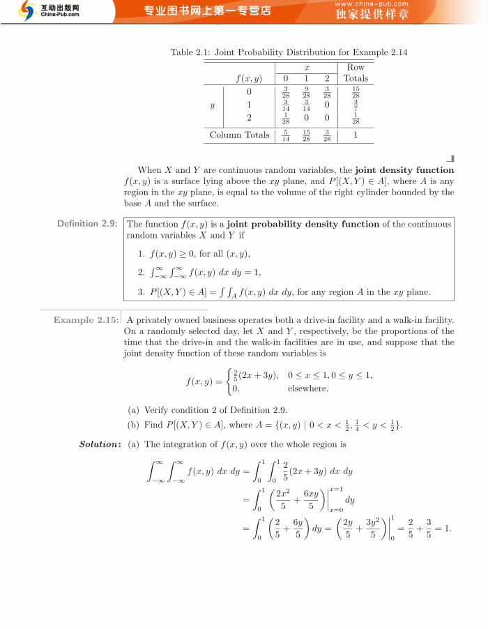
Table 2.1: Joint Probability Distribution for Example 2.14

x Rowf(x, y) 0 1 2 Totals

0 328

928

328

1528

y 1 314

314 0 3

7

2 128 0 0 1

28

Column Totals 514

1528

328 1

When X and Y are continuous random variables, the joint density functionf(x, y) is a surface lying above the xy plane, and P [(X,Y ) ∈ A], where A is anyregion in the xy plane, is equal to the volume of the right cylinder bounded by thebase A and the surface.

Definition 2.9: The function f(x, y) is a joint probability density function of the continuousrandom variables X and Y if

1. f(x, y) ≥ 0, for all (x, y),

2.∫∞−∞

∫∞−∞ f(x, y) dx dy = 1,

3. P [(X,Y ) ∈ A] =∫ ∫

Af(x, y) dx dy, for any region A in the xy plane.

Example 2.15: A privately owned business operates both a drive-in facility and a walk-in facility.On a randomly selected day, let X and Y , respectively, be the proportions of thetime that the drive-in and the walk-in facilities are in use, and suppose that thejoint density function of these random variables is

f(x, y) =

{25 (2x+ 3y), 0 ≤ x ≤ 1, 0 ≤ y ≤ 1,

0, elsewhere.

(a) Verify condition 2 of Definition 2.9.

(b) Find P [(X,Y ) ∈ A], where A = {(x, y) | 0 < x < 12 ,

14 < y < 1

2}.

Solution : (a) The integration of f(x, y) over the whole region is∫ ∞

−∞

∫ ∞

−∞f(x, y) dx dy =

∫ 1

0

∫ 1

0

2

5(2x+ 3y) dx dy

=

∫ 1

0

(2x2

5+

6xy

5

)∣∣∣∣x=1

x=0

dy

=

∫ 1

0

(2

5+

6y

5

)dy =

(2y

5+

3y2

5

)∣∣∣∣10

=2

5+

3

5= 1.

ii


ii

ii


(b) To calculate the probability, we use

P [(X,Y ) ∈ A] = P

(0 < X <

1

2,1

4< Y <

1

2

)=

∫ 1/2

1/4

∫ 1/2

0

2

5(2x+ 3y) dx dy

=

∫ 1/2

1/4

(2x2

5+

6xy

5

)∣∣∣∣x=1/2

x=0

dy =

∫ 1/2

1/4

(1

10+

3y

5

)dy

=

(y

10+

3y2

10

)∣∣∣∣1/21/4

=1

10

[(1

2+

3

4

)−(1

4+

3

16

)]=

13

160.

Given the joint probability distribution f(x, y) of the discrete random variablesX and Y , the probability distribution g(x) of X alone is obtained by summingf(x, y) over all the values of Y at each value of x. Similarly, the probabilitydistribution h(y) of Y alone is obtained by summing f(x, y) over the values ofX. We define g(x) and h(y) to be the marginal distributions of X and Y ,respectively. When X and Y are continuous random variables, summations arereplaced by integrals. We can now make the following general definition.

Definition 2.10: The marginal distributions of X alone and of Y alone are

g(x) =∑y

f(x, y) and h(y) =∑x

f(x, y)

for the discrete case, and

g(x) =

∫ ∞

−∞f(x, y) dy and h(y) =

∫ ∞

−∞f(x, y) dx

for the continuous case.

The term marginal is used here because, in the discrete case, the values of g(x)and h(y) are just the marginal totals of the respective columns and rows when thevalues of f(x, y) are displayed in a rectangular table.

Example 2.16: Show that the column and row totals of Table 2.1 give the marginal distributionof X alone and of Y alone.

Solution : For the random variable X, we see that

g(0) = f(0, 0) + f(0, 1) + f(0, 2) =3

28+

3

14+

1

28=

5

14,

g(1) = f(1, 0) + f(1, 1) + f(1, 2) =9

28+

3

14+ 0 =

15

28,

and

g(2) = f(2, 0) + f(2, 1) + f(2, 2) =3

28+ 0 + 0 =

3

28,

ii


ii

ii


which are just the column totals of Table 2.1. In a similar manner we could showthat the values of h(y) are given by the row totals. In tabular form, these marginaldistributions may be written as follows:

x 0 1 2

g(x) 514

1528

328

y 0 1 2

h(y) 1528

37

128

Example 2.17: Find g(x) and h(y) for the joint density function of Example 2.15.Solution : By definition,

g(x) =

∫ ∞

−∞f(x, y) dy =

∫ 1

0

2

5(2x+ 3y) dy =

(4xy

5+

6y2

10

)∣∣∣∣y=1

y=0

=4x+ 3

5,

for 0 ≤ x ≤ 1, and g(x) = 0 elsewhere. Similarly,

h(y) =

∫ ∞

−∞f(x, y) dx =

∫ 1

0

2

5(2x+ 3y) dx =

2(1 + 3y)

5,

for 0 ≤ y ≤ 1, and h(y) = 0 elsewhere.The fact that the marginal distributions g(x) and h(y) are indeed the proba-

bility distributions of the individual variables X and Y alone can be verified byshowing that the conditions of Definition 2.4 or Definition 2.6 are satisfied. Forexample, in the continuous case∫ ∞

−∞g(x) dx =

∫ ∞

−∞

∫ ∞

−∞f(x, y) dy dx = 1,

and

P (a < X < b) = P (a < X < b,−∞ < Y < ∞)

=

∫ b

a

∫ ∞

−∞f(x, y) dy dx =

∫ b

a

g(x) dx.

In Section 2.1, we stated that the value x of the random variable X representsan event that is a subset of the sample space. If we use the definition of conditionalprobability as stated in Chapter 1,

P (B|A) =P (A ∩B)

P (A), provided P (A) > 0,

where A and B are now the events defined by X = x and Y = y, respectively, then

P (Y = y | X = x) =P (X = x, Y = y)

P (X = x)=

f(x, y)

g(x), provided g(x) > 0,

where X and Y are discrete random variables.It is not difficult to show that the function f(x, y)/g(x), which is strictly a func-

tion of y with x fixed, satisfies all the conditions of a probability distribution. Thisis also true when f(x, y) and g(x) are the joint density and marginal distribution,respectively, of continuous random variables. As a result, it is extremely important

ii


ii

ii


that we make use of the special type of distribution of the form f(x, y)/g(x) inorder to be able to effectively compute conditional probabilities. This type of dis-tribution is called a conditional probability distribution; the formal definitionfollows.

Definition 2.11: Let X and Y be two random variables, discrete or continuous. The conditionaldistribution of the random variable Y given that X = x is

f(y|x) = f(x, y)

g(x), provided g(x) > 0.

Similarly, the conditional distribution of X given that Y = y is

f(x|y) = f(x, y)

h(y), provided h(y) > 0.

If we wish to find the probability that the discrete random variable X falls betweena and b when it is known that the discrete variable Y = y, we evaluate

P (a < X < b | Y = y) =∑

a<x<b

f(x|y),

where the summation extends over all values of X between a and b. When X andY are continuous, we evaluate

P (a < X < b | Y = y) =

∫ b

a

f(x|y) dx.

Example 2.18: Referring to Example 2.14, find the conditional distribution of X, given thatY = 1, and use it to determine P (X = 0 | Y = 1).

Solution : We need to find f(x|y), where y = 1. First, we find that

h(1) =

2∑x=0

f(x, 1) =3

14+

3

14+ 0 =

3

7.

Now

f(x|1) = f(x, 1)

h(1)=

(7

3

)f(x, 1), x = 0, 1, 2.

Therefore,

f(0|1) =(7

3

)f(0, 1) =

(7

3

)(3

14

)=

1

2, f(1|1) =

(7

3

)f(1, 1) =

(7

3

)(3

14

)=

1

2,

f(2|1) =(7

3

)f(2, 1) =

(7

3

)(0) = 0,

and the conditional distribution of X, given that Y = 1, is

ii


ii

ii


x 0 1 2

f(x|1) 12

12 0

Finally,

P (X = 0 | Y = 1) = f(0|1) = 1

2.

Therefore, if it is known that 1 of the 2 pens selected is red, we have a probabilityequal to 1/2 that the other pen is not blue.

Example 2.19: The joint density for the random variables (X,Y ), where X is the temperaturechange and Y is the proportion of the spectrum that shifts for a certain atomicparticle, is

f(x, y) =

{10xy2, 0 < x < y < 1,

0, elsewhere.

(a) Find the marginal densities g(x), h(y), and the conditional density f(y|x).(b) Find the probability that the spectrum shifts more than half of the total

observations, given that the temperature is increased by 0.25 unit.

Solution : (a) By definition,

g(x) =

∫ ∞

−∞f(x, y) dy =

∫ 1

x

10xy2 dy

=10

3xy3∣∣∣∣y=1

y=x

=10

3x(1− x3), 0 < x < 1,

h(y) =

∫ ∞

−∞f(x, y) dx =

∫ y

0

10xy2 dx = 5x2y2∣∣x=y

x=0= 5y4, 0 < y < 1.

Now

f(y|x) = f(x, y)

g(x)=

10xy2

103 x(1− x3)

=3y2

1− x3, 0 < x < y < 1.

(b) Therefore,

P

(Y >

1

2

∣∣∣∣ X = 0.25

)=

∫ 1

1/2

f(y | x = 0.25) dy =

∫ 1

1/2

3y2

1− 0.253dy =

8

9.

Example 2.20: Given the joint density function

f(x, y) =

{x(1+3y2)

4 , 0 < x < 2, 0 < y < 1,

0, elsewhere,

find g(x), h(y), f(x|y), and evaluate P ( 14 < X < 12 | Y = 1

3 ).Solution : By the definition of the marginal density, for 0 < x < 2,

g(x) =

∫ ∞

−∞f(x, y) dy =

∫ 1

0

x(1 + 3y2)

4dy

=

(xy

4+

xy3

4

)∣∣∣∣y=1

y=0

=x

2,

ii


ii

ii


and for 0 < y < 1,

h(y) =

∫ ∞

−∞f(x, y) dx =

∫ 2

0

x(1 + 3y2)

4dx

=

(x2

8+

3x2y2

8

)∣∣∣∣x=2

x=0

=1 + 3y2

2.

Therefore, using the conditional density definition, for 0 < x < 2,

f(x|y) = f(x, y)

h(y)=

x(1 + 3y2)/4

(1 + 3y2)/2=

x

2,

and

P

(1

4< X <

1

2

∣∣∣∣ Y =1

3

)=

∫ 1/2

1/4

x

2dx =

3

64.

Statistical Independence

If f(x|y) does not depend on y, as is the case for Example 2.20, then f(x|y) = g(x)and f(x, y) = g(x)h(y). The proof follows by substituting

f(x, y) = f(x|y)h(y)

into the marginal distribution of X. That is,

g(x) =

∫ ∞

−∞f(x, y) dy =

∫ ∞

−∞f(x|y)h(y) dy.

If f(x|y) does not depend on y, we may write

g(x) = f(x|y)∫ ∞

−∞h(y) dy.

Now ∫ ∞

−∞h(y) dy = 1,

since h(y) is the probability density function of Y . Therefore,

g(x) = f(x|y) and then f(x, y) = g(x)h(y).

It should make sense to the reader that if f(x|y) does not depend on y, then ofcourse the outcome of the random variable Y has no impact on the outcome of therandom variable X. In other words, we say that X and Y are independent randomvariables. We now offer the following formal definition of statistical independence.

ii


ii

ii


Definition 2.12: Let X and Y be two random variables, discrete or continuous, with joint proba-bility distribution f(x, y) and marginal distributions g(x) and h(y), respectively.The random variables X and Y are said to be statistically independent if andonly if

f(x, y) = g(x)h(y)

for all (x, y) within their range.

The continuous random variables of Example 2.20 are statistically indepen-dent, since the product of the two marginal distributions gives the joint densityfunction. This is obviously not the case, however, for the continuous variables ofExample 2.19. Checking for statistical independence of discrete random variablesrequires a more thorough investigation, since it is possible to have the product ofthe marginal distributions equal to the joint probability distribution for some butnot all combinations of (x, y). If you can find any point (x, y) for which f(x, y)is defined such that f(x, y) = g(x)h(y), the discrete variables X and Y are notstatistically independent.

Example 2.21: Show that the random variables of Example 2.14 are not statistically independent.Proof : Let us consider the point (0, 1). From Table 2.1 we find the three probabilities

f(0, 1), g(0), and h(1) to be

f(0, 1) =3

14,

g(0) =2∑

y=0

f(0, y) =3

28+

3

14+

1

28=

5

14,

h(1) =

2∑x=0

f(x, 1) =3

14+

3

14+ 0 =

3

7.

Clearly,

f(0, 1) = g(0)h(1),

and therefore X and Y are not statistically independent.All the preceding definitions concerning two random variables can be general-

ized to the case of n random variables. Let f(x1, x2, . . . , xn) be the joint probabilityfunction of the random variables X1, X2, . . . , Xn. The marginal distribution of X1,for example, is

g(x1) =∑x2

· · ·∑xn

f(x1, x2, . . . , xn)

for the discrete case, and

g(x1) =

∫ ∞

−∞· · ·∫ ∞

−∞f(x1, x2, . . . , xn) dx2 dx3 · · · dxn

ii


ii

ii


for the continuous case. We can now obtain joint marginal distributions suchas g(x1, x2), where

g(x1, x2) =

∑x3

· · ·∑xn

f(x1, x2, . . . , xn) (discrete case),∫∞−∞ · · ·

∫∞−∞ f(x1, x2, . . . , xn) dx3 dx4 · · · dxn (continuous case).

We could consider numerous conditional distributions. For example, the joint con-ditional distribution of X1, X2, and X3, given that X4 = x4, X5 = x5, . . . , Xn =xn, is written

f(x1, x2, x3 | x4, x5, . . . , xn) =f(x1, x2, . . . , xn)

g(x4, x5, . . . , xn),

where g(x4, x5, . . . , xn) is the joint marginal distribution of the random variablesX4, X5, . . . , Xn.

A generalization of Definition 2.12 leads to the following definition for the mu-tual statistical independence of the variables X1, X2, . . . , Xn.

Definition 2.13: Let X1, X2, . . . , Xn be n random variables, discrete or continuous, withjoint probability distribution f(x1, x2, . . . , xn) and marginal distributionf1(x1), f2(x2), . . . , fn(xn), respectively. The random variablesX1, X2, . . . , Xn aresaid to be mutually statistically independent if and only if

f(x1, x2, . . . , xn) = f1(x1)f2(x2) · · · fn(xn)

for all (x1, x2, . . . , xn) within their range.

Example 2.22: Suppose that the shelf life, in years, of a certain perishable food product packagedin cardboard containers is a random variable whose probability density function isgiven by

f(x) =

{e−x, x > 0,

0, elsewhere.

Let X1, X2, and X3 represent the shelf lives for three of these containers selectedindependently and find P (X1 < 2, 1 < X2 < 3, X3 > 2).

Solution : Since the containers were selected independently, we can assume that the randomvariables X1, X2, and X3 are statistically independent, having the joint probabilitydensity

f(x1, x2, x3) = f(x1)f(x2)f(x3) = e−x1e−x2e−x3 = e−x1−x2−x3 ,

for x1 > 0, x2 > 0, x3 > 0, and f(x1, x2, x3) = 0 elsewhere. Hence

P (X1 < 2, 1 < X2 < 3, X3 > 2) =

∫ ∞

2

∫ 3

1

∫ 2

0

e−x1−x2−x3 dx1 dx2 dx3

= (1− e−2)(e−1 − e−3)e−2 = 0.0372.

ii


ii

ii


What Are Important Characteristics of Probability Distributionsand Where Do They Come From?

This is an important point in the text to provide the reader with a transition intothe next three chapters. We have given illustrations in both examples and exercisesof practical scientific and engineering situations in which probability distributionsand their properties are used to solve important problems. These probability dis-tributions, either discrete or continuous, were introduced through phrases like “it isknown that” or “suppose that” or even in some cases “historical evidence suggeststhat.” These are situations in which the nature of the distribution and even a goodestimate of the probability structure can be determined through historical data,data from long-term studies, or even large amounts of planned data. However, notall probability functions and probability density functions are derived from largeamounts of historical data. There are a substantial number of situations in whichthe nature of the scientific scenario suggests a distribution type. For example,when independent repeated observations are binary in nature (e.g., defective ornot, survive or not, allergic or not) with value 0 or 1, the distribution coveringthis situation is called the binomial distribution and the probability function isknown and will be demonstrated in its generality in Chapter 3.

A second part of this transition to material in future chapters deals with thenotion of population parameters or distributional parameters. We willdiscuss later in this chapter the notions of a mean and variance and provide avision for the concepts in the context of a population. Indeed, the population meanand variance are easily found from the probability function for the discrete caseor the probability density function for the continuous case. These parameters andtheir importance in the solution of many types of real-world problems will providemuch of the material in Chapters 4 through 9.

Exercises

2.29 Determine the values of c so that the follow-ing functions represent joint probability distributionsof the random variables X and Y :

(a) f(x, y) = cxy, for x = 1, 2, 3; y = 1, 2, 3;

(b) f(x, y) = c|x− y|, for x = −2, 0, 2; y = −2, 3.

2.30 If the joint probability distribution of X and Yis given by

f(x, y) =x+ y

30, for x = 0, 1, 2, 3; y = 0, 1, 2,

find

(a) P (X ≤ 2, Y = 1);

(b) P (X > 2, Y ≤ 1);

(c) P (X > Y );

(d) P (X + Y = 4).

(e) Find the marginal distribution of X; of Y .

2.31 From a sack of fruit containing 3 oranges, 2 ap-ples, and 3 bananas, a random sample of 4 pieces offruit is selected. If X is the number of oranges and Yis the number of apples in the sample, find

(a) the joint probability distribution of X and Y ;

(b) P [(X,Y ) ∈ A], where A is the region that is givenby {(x, y) | x+ y ≤ 2};

(c) P (Y = 0 | X = 2);

(d) the conditional distribution of y, given X = 2.

2.32 A fast-food restaurant operates both a drive-through facility and a walk-in facility. On a randomlyselected day, let X and Y , respectively, be the propor-tions of the time that the drive-through and walk-infacilities are in use, and suppose that the joint densityfunction of these random variables is

f(x, y) =

{23(x+ 2y), 0 ≤ x ≤ 1, 0 ≤ y ≤ 1,

0, elsewhere.

ii


ii

ii

Exercises 73

(a) Find the marginal density of X.

(b) Find the marginal density of Y .

(c) Find the probability that the drive-through facilityis busy less than one-half of the time.

2.33 A candy company distributes boxes of choco-lates with a mixture of creams, toffees, and cordials.Suppose that the weight of each box is 1 kilogram, butthe individual weights of the creams, toffees, and cor-dials vary from box to box. For a randomly selectedbox, let X and Y represent the weights of the creamsand the toffees, respectively, and suppose that the jointdensity function of these variables is

f(x, y) =

{24xy, 0 ≤ x ≤ 1, 0 ≤ y ≤ 1, x+ y ≤ 1,

0, elsewhere.

(a) Find the probability that in a given box the cordialsaccount for more than 1/2 of the weight.

(b) Find the marginal density for the weight of thecreams.

(c) Find the probability that the weight of the toffeesin a box is less than 1/8 of a kilogram if it is knownthat creams constitute 3/4 of the weight.

2.34 Let X and Y denote the lengths of life, in years,of two components in an electronic system. If the jointdensity function of these variables is

f(x, y) =

{e−(x+y), x > 0, y > 0,

0, elsewhere,

find P (0 < X < 1 | Y = 2).

2.35 Let X denote the reaction time, in seconds, toa certain stimulus and Y denote the temperature (◦F)at which a certain reaction starts to take place. Sup-pose that two random variables X and Y have the jointdensity

f(x, y) =

{4xy, 0 < x < 1, 0 < y < 1,

0, elsewhere.

Find

(a) P (0 ≤ X ≤ 12and 1

4≤ Y ≤ 1

2);

(b) P (X < Y ).

2.36 Each rear tire on an experimental airplane issupposed to be filled to a pressure of 40 pounds persquare inch (psi). Let X denote the actual air pressurefor the right tire and Y denote the actual air pressurefor the left tire. Suppose that X and Y are randomvariables with the joint density function

f(x, y) =

{k(x2 + y2), 30 ≤ x < 50, 30 ≤ y < 50,

0, elsewhere.

(a) Find k.

(b) Find P (30 ≤ X ≤ 40 and 40 ≤ Y < 50).

(c) Find the probability that both tires are underfilled.

2.37 Let X denote the diameter of an armored elec-tric cable and Y denote the diameter of the ceramicmold that makes the cable. Both X and Y are scaledso that they range between 0 and 1. Suppose that Xand Y have the joint density

f(x, y) =

{1y, 0 < x < y < 1,

0, elsewhere.

Find P (X + Y > 1/2).

2.38 The amount of kerosene, in thousands of liters,in a tank at the beginning of any day is a randomamount Y from which a random amount X is sold dur-ing that day. Suppose that the tank is not resuppliedduring the day so that x ≤ y, and assume that thejoint density function of these variables is

f(x, y) =

{2, 0 < x ≤ y < 1,

0, elsewhere.

(a) Determine if X and Y are independent.

(b) Find P (1/4 < X < 1/2 | Y = 3/4).

2.39 Let X denote the number of times a certain nu-merical control machine will malfunction: 1, 2, or 3times on any given day. Let Y denote the number oftimes a technician is called on an emergency call. Theirjoint probability distribution is given as

xf(x, y) 1 2 3

y135

0.050.050.00

0.050.100.20

0.100.350.10

(a) Evaluate the marginal distribution of X.

(b) Evaluate the marginal distribution of Y .

(c) Find P (Y = 3 | X = 2).

2.40 Suppose that X and Y have the following jointprobability distribution:

xf(x, y) 2 4

1 0.10 0.15y 3 0.20 0.30

5 0.10 0.15

(a) Find the marginal distribution of X.

(b) Find the marginal distribution of Y .

ii


ii

ii


2.41 Given the joint density function

f(x, y) =

{ 6−x−y8

, 0 < x < 2, 2 < y < 4,

0, elsewhere,

find P (1 < Y < 3 | X = 1).

2.42 A coin is tossed twice. Let Z denote the numberof heads on the first toss and W the total number ofheads on the 2 tosses. If the coin is unbalanced and ahead has a 40% chance of occurring, find

(a) the joint probability distribution of W and Z;

(b) the marginal distribution of W ;

(c) the marginal distribution of Z;

(d) the probability that at least 1 head occurs.

2.43 Determine whether the two random variables ofExercise 2.40 are dependent or independent.


2.45 Let X, Y , and Z have the joint probability den-sity function

f(x, y, z) =

{kxy2z, 0 < x, y < 1, 0 < z < 2,

0, elsewhere.

(a) Find k.

(b) Find P (X < 14, Y > 1

2, 1 < Z < 2).

2.46 The joint density function of the random vari-ables X and Y is

f(x, y) =

{6x, 0 < x < 1, 0 < y < 1− x,

0, elsewhere.

(a) Show that X and Y are not independent.

(b) Find P (X > 0.3 | Y = 0.5).


2.48 The joint probability density function of the ran-dom variables X, Y , and Z is

f(x, y, z) =

{4xyz2

9, 0 < x, y < 1, 0 < z < 3,

0, elsewhere.

Find

(a) the joint marginal density function of Y and Z;

(b) the marginal density of Y ;

(c) P ( 14< X < 1

2, Y > 1

3, 1 < Z < 2);

(d) P (0 < X < 12| Y = 1

4, Z = 2).


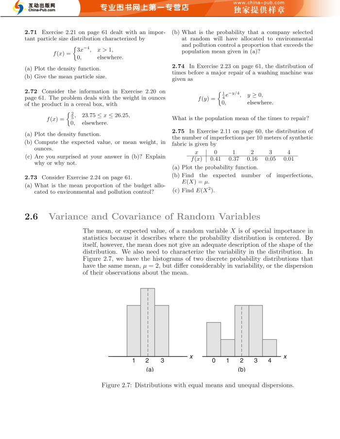
2.5 Mean of a Random Variable

We can refer to the population mean of the random variable X or the meanof the probability distribution of X and write it as µx, or simply as µ when itis clear to which random variable we refer. It is also common among statisticiansto refer to this mean as the mathematical expectation, or the expected value ofthe random variable X, and denote it as E(X).

Assuming that one fair coin was tossed twice, we find that the sample space forour experiment is

S = {HH,HT, TH, TT}.

Denote by X the number of heads. Since the 4 sample points are all equally likely,it follows that

P (X = 0) = P (TT ) =1

4, P (X = 1) = P (TH) + P (HT ) =

1

2,

and

P (X = 2) = P (HH) =1

4,

ii


ii

ii

2.5 Mean of a Random Variable 75

where a typical element, say TH, indicates that the first toss resulted in a tailfollowed by a head on the second toss. Now, these probabilities are just the relativefrequencies for the given events in the long run. Therefore,

µ = E(X) = (0)

(1

4

)+ (1)

(1

2

)+ (2)

(1

4

)= 1.

This result means that a person who tosses 2 coins over and over again will, on theaverage, get 1 head per toss.

Definition 2.14: Let X be a random variable with probability distribution f(x). The mean, orexpected value, of X is

µ = E(X) =∑x

xf(x)

if X is discrete, and

µ = E(X) =

∫ ∞

−∞xf(x) dx

if X is continuous.

Example 2.23: A lot containing 7 components is sampled by a quality inspector; the lot contains4 good components and 3 defective components. A sample of 3 is taken by theinspector. Find the expected value of the number of good components in thissample.

Solution : Let X represent the number of good components in the sample. The probabilitydistribution of X is

f(x) =

(4x

)(3

3−x

)(73

) , x = 0, 1, 2, 3.

Simple calculations yield f(0) = 1/35, f(1) = 12/35, f(2) = 18/35, and f(3) =4/35. Therefore,

µ = E(X) = (0)

(1

35

)+ (1)

(12

35

)+ (2)

(18

35

)+ (3)

(4

35

)=

12

7= 1.7.

Thus, if a sample of size 3 is selected at random over and over again from a lotof 4 good components and 3 defective components, it will contain, on average, 1.7good components.

Example 2.24: A salesperson for a medical device company has two appointments on a givenday. At the first appointment, he believes that he has a 70% chance to make thedeal, from which he can earn $1000 commission if successful. On the other hand,he thinks he only has a 40% chance to make the deal at the second appointment,from which, if successful, he can make $1500. What is his expected commissionbased on his own probability belief? Assume that the appointment results areindependent of each other.

ii


ii

ii


Solution : First, we know that the salesperson, for the two appointments, can have 4 possiblecommission totals: $0, $1000, $1500, and $2500. We then need to calculate theirassociated probabilities. By independence, we obtain

f($0) = (1− 0.7)(1− 0.4) = 0.18, f($2500) = (0.7)(0.4) = 0.28,

f($1000) = (0.7)(1− 0.4) = 0.42, and f($1500) = (1− 0.7)(0.4) = 0.12.

Therefore, the expected commission for the salesperson is

E(X) = ($0)(0.18) + ($1000)(0.42) + ($1500)(0.12) + ($2500)(0.28)

= $1300.Examples 2.23 and 2.24 are designed to allow the reader to gain some insight

into what we mean by the expected value of a random variable. In both cases therandom variables are discrete. We follow with an example involving a continuousrandom variable, where an engineer is interested in the mean life of a certaintype of electronic device. This is an illustration of a time to failure problem thatoccurs often in practice. The expected value of the life of a device is an importantparameter for its evaluation.

Example 2.25: Let X be the random variable that denotes the life in hours of a certain electronicdevice. The probability density function is

f(x) =

{20,000x3 , x > 100,

0, elsewhere.

Find the expected life of this type of device.Solution : Using Definition 2.14, we have

µ = E(X) =

∫ ∞

100

x20, 000

x3dx =

∫ ∞

100

20, 000

x2dx = 200.

Therefore, we can expect this type of device to last, on average, 200 hours.Now let us consider a new random variable g(X), which depends on X; that

is, each value of g(X) is determined by the value of X. For instance, g(X) mightbe X2 or 3X − 1, and whenever X assumes the value 2, g(X) assumes the valueg(2). In particular, if X is a discrete random variable with probability distributionf(x), for x = −1, 0, 1, 2, and g(X) = X2, then

P [g(X) = 0] = P (X = 0) = f(0),

P [g(X) = 1] = P (X = −1) + P (X = 1) = f(−1) + f(1),

P [g(X) = 4] = P (X = 2) = f(2),

and so the probability distribution of g(X) may be written

g(x) 0 1 4P [g(X) = g(x)] f(0) f(−1) + f(1) f(2)

By the definition of the expected value of a random variable, we obtain

µg(X) = E[g(x)] = 0f(0) + 1[f(−1) + f(1)] + 4f(2)

= (−1)2f(−1) + (0)2f(0) + (1)2f(1) + (2)2f(2) =∑x

g(x)f(x).

ii


ii

ii

2.5 Mean of a Random Variable 77

This result is generalized in Theorem 2.1 for both discrete and continuous randomvariables.

Theorem 2.1: Let X be a random variable with probability distribution f(x). The expectedvalue of the random variable g(X) is

µg(X) = E[g(X)] =∑x

g(x)f(x)


µg(X) = E[g(X)] =

∫ ∞

−∞g(x)f(x) dx

if X is continuous.

Example 2.26: Suppose that the number of cars X that pass through a car wash between 4:00P.M. and 5:00 P.M. on any sunny Friday has the following probability distribution:

x 4 5 6 7 8 9

P (X = x) 112

112

14

14

16

16

Let g(X) = 2X−1 represent the amount of money, in dollars, paid to the attendantby the manager. Find the attendant’s expected earnings for this particular timeperiod.

Solution : By Theorem 2.1, the attendant can expect to receive

E[g(X)] = E(2X − 1) =

9∑x=4

(2x− 1)f(x)

= (7)

(1

12

)+ (9)

(1

12

)+ (11)

(1

4

)+ (13)

(1

4

)+ (15)

(1

6

)+ (17)

(1

6

)= $12.67.

Example 2.27: Let X be a random variable with density function

f(x) =

{x2

3 , −1 < x < 2,

0, elsewhere.

Find the expected value of g(X) = 4X + 3.Solution : By Theorem 2.1, we have

E(4X + 3) =

∫ 2

−1

(4x+ 3)x2

3dx =

1

3

∫ 2

−1

(4x3 + 3x2) dx = 8.

We shall now extend our concept of mathematical expectation to the case oftwo random variables X and Y with joint probability distribution f(x, y).

ii


ii

ii


Definition 2.15: Let X and Y be random variables with joint probability distribution f(x, y). Themean, or expected value, of the random variable g(X,Y ) is

µg(X,Y ) = E[g(X,Y )] =∑x

∑y

g(x, y)f(x, y)

if X and Y are discrete, and

µg(X,Y ) = E[g(X,Y )] =

∫ ∞

−∞

∫ ∞

−∞g(x, y)f(x, y) dx dy

if X and Y are continuous.

Generalization of Definition 2.15 for the calculation of mathematical expecta-tions of functions of several random variables is straightforward.

Example 2.28: Let X and Y be the random variables with joint probability distribution indicatedin Table 2.1 on page 64. Find the expected value of g(X,Y ) = XY . The table isreprinted here for convenience.

x Rowf(x, y) 0 1 2 Totals

0 3/28 9/28 3/28 15/28

y 1 3/14 3/14 0 3/7

2 1/28 0 0 1/28

Column Totals 5/14 15/28 3/28 1

Solution : By Definition 2.15, we write

E(XY ) =2∑

x=0

2∑y=0

xyf(x, y)

= (0)(0)f(0, 0) + (0)(1)f(0, 1)

+ (1)(0)f(1, 0) + (1)(1)f(1, 1) + (2)(0)f(2, 0)

= f(1, 1) =3

14.

Example 2.29: Find E(Y/X) for the density function

f(x, y) =

{x(1+3y2)

4 , 0 < x < 2, 0 < y < 1,

0, elsewhere.

Solution : We have

E

(Y

X

)=

∫ 1

0

∫ 2

0

y(1 + 3y2)

4dx dy =

∫ 1

0

y + 3y3

2dy =

5

8.

ii


ii

ii

Exercises 79

Note that if g(X,Y ) = X in Definition 2.15, we have

E(X) =

∑x

∑yxf(x, y) =

∑xxg(x) (discrete case),∫∞

−∞∫∞−∞ xf(x, y) dy dx =

∫∞−∞ xg(x) dx (continuous case),

where g(x) is the marginal distribution of X. Therefore, in calculating E(X) overa two-dimensional space, one may use either the joint probability distribution ofX and Y or the marginal distribution of X. Similarly, we define

E(Y ) =

∑y

∑xyf(x, y) =

∑yyh(y) (discrete case),∫∞

−∞∫∞−∞ yf(x, y) dx dy =

∫∞−∞ yh(y) dy (continuous case),

where h(y) is the marginal distribution of the random variable Y .

Exercises

2.50 The probability distribution of the discrete ran-dom variable X is

f(x) =

(3

x

)(1

4

)x(3

4

)3−x

, x = 0, 1, 2, 3.

Find the mean of X.

2.51 The probability distribution of X, the numberof imperfections per 10 meters of a synthetic fabric incontinuous rolls of uniform width, is given in Exercise2.11 on page 60 as

x 0 1 2 3 4f(x) 0.41 0.37 0.16 0.05 0.01

Find the average number of imperfections per 10 me-ters of this fabric.

2.52 A coin is biased such that a head is three timesas likely to occur as a tail. Find the expected numberof tails when this coin is tossed twice.

2.53 Find the mean of the random variable T repre-senting the total of the three coins in Exercise 2.17 onpage 61.

2.54 In a gambling game, a woman is paid $3 if shedraws a jack or a queen and $5 if she draws a king oran ace from an ordinary deck of 52 playing cards. Ifshe draws any other card, she loses. How much shouldshe pay to play if the game is fair?

2.55 By investing in a particular stock, a person canmake a profit in one year of $4000 with probability 0.3or take a loss of $1000 with probability 0.7. What isthis person’s expected gain?

2.56 Suppose that an antique jewelry dealer is inter-ested in purchasing a gold necklace for which the prob-abilities are 0.22, 0.36, 0.28, and 0.14, respectively, thatshe will be able to sell it for a profit of $250, sell it fora profit of $150, break even, or sell it for a loss of $150.What is her expected profit?

2.57 The density function of coded measurements ofthe pitch diameter of threads of a fitting is

f(x) =

{4

π(1+x2), 0 < x < 1,

0, elsewhere.

Find the expected value of X.

2.58 Two tire-quality experts examine stacks of tiresand assign a quality rating to each tire on a 3-pointscale. Let X denote the rating given by expert A andY denote the rating given by B. The following tablegives the joint distribution for X and Y .

yf(x, y) 1 2 3

1 0.10 0.05 0.02x 2 0.10 0.35 0.05

3 0.03 0.10 0.20

Find µX and µY .

2.59 The density function of the continuous randomvariable X, the total number of hours, in units of 100hours, that a family runs a vacuum cleaner over a pe-riod of one year, is given in Exercise 2.7 on page 60

ii


ii

ii


as

f(x) =

x, 0 < x < 1,

2− x, 1 ≤ x < 2,

0, elsewhere.

Find the average number of hours per year that familiesrun their vacuum cleaners.

2.60 If a dealer’s profit, in units of $5000, on a newautomobile can be looked upon as a random variableX having the density function

f(x) =

{2(1− x), 0 < x < 1,

0, elsewhere,

find the average profit per automobile.

2.61 Assume that two random variables (X,Y ) areuniformly distributed on a circle with radius a. Thenthe joint probability density function is

f(x, y) =

{1

πa2 , x2 + y2 ≤ a2,

0, otherwise.

Find µX , the expected value of X.

2.62 Find the proportion X of individuals who can beexpected to respond to a certain mail-order solicitationif X has the density function

f(x) =

{2(x+2)

5, 0 < x < 1,

0, elsewhere.

2.63 Let X be a random variable with the followingprobability distribution:

x −3 6 9f(x) 1/6 1/2 1/3

Find µg(X), where g(X) = (2X + 1)2.

2.64 Suppose that you are inspecting a lot of 1000light bulbs, among which 20 are defectives. You choosetwo light bulbs randomly from the lot without replace-ment. Let

X1 =

{1, if the 1st light bulb is defective,

0, otherwise,

X2 =

{1, if the 2nd light bulb is defective,

0, otherwise.

Find the probability that at least one light bulb chosenis defective. [Hint: Compute P (X1 +X2 = 1).]

2.65 A large industrial firm purchases several newword processors at the end of each year, the exact num-ber depending on the frequency of repairs in the previ-ous year. Suppose that the number of word processors,X, purchased each year has the following probabilitydistribution:

x 0 1 2 3f(x) 1/10 3/10 2/5 1/5

If the cost of the desired model is $1200 per unit andat the end of the year a refund of 50X2 dollars will beissued, how much can this firm expect to spend on newword processors during this year?

2.66 The hospitalization period, in days, for patientsfollowing treatment for a certain type of kidney disor-der is a random variable Y = X + 4, where X has thedensity function

f(x) =

{32

(x+4)3, x > 0,

0, elsewhere.

Find the average number of days that a person is hos-pitalized following treatment for this disorder.

2.67 Suppose that X and Y have the following jointprobability function:

xf(x, y) 2 4

1 0.10 0.15y 3 0.20 0.30

5 0.10 0.15

(a) Find the expected value of g(X,Y ) = XY 2.

(b) Find µX and µY .

2.68 Referring to the random variables whose jointprobability distribution is given in Exercise 2.31 onpage 72,

(a) find E(X2Y − 2XY );

(b) find µX − µY .

2.69 In Exercise 2.19 on page 61, a density functionis given for the time to failure of an important compo-nent of a DVD player. Find the mean number of hoursto failure of the component and thus the DVD player.

2.70 Let X and Y be random variables with jointdensity function

f(x, y) =

{4xy, 0 < x, y < 1,

0, elsewhere.

Find the expected value of Z =√X2 + Y 2.

ii


ii

ii

2.6 Variance and Covariance of Random Variables 81

2.71 Exercise 2.21 on page 61 dealt with an impor-tant particle size distribution characterized by

f(x) =

{3x−4, x > 1,

0, elsewhere.

(a) Plot the density function.

(b) Give the mean particle size.

2.72 Consider the information in Exercise 2.20 onpage 61. The problem deals with the weight in ouncesof the product in a cereal box, with

f(x) =

{25, 23.75 ≤ x ≤ 26.25,

0, elsewhere.

(a) Plot the density function.

(b) Compute the expected value, or mean weight, inounces.

(c) Are you surprised at your answer in (b)? Explainwhy or why not.

2.73 Consider Exercise 2.24 on page 61.

(a) What is the mean proportion of the budget allo-cated to environmental and pollution control?

(b) What is the probability that a company selectedat random will have allocated to environmentaland pollution control a proportion that exceeds thepopulation mean given in (a)?

2.74 In Exercise 2.23 on page 61, the distribution oftimes before a major repair of a washing machine wasgiven as

f(y) =

{14e−y/4, y ≥ 0,

0, elsewhere.

What is the population mean of the times to repair?

2.75 In Exercise 2.11 on page 60, the distribution ofthe number of imperfections per 10 meters of syntheticfabric is given by

x 0 1 2 3 4f(x) 0.41 0.37 0.16 0.05 0.01

(a) Plot the probability function.

(b) Find the expected number of imperfections,E(X) = µ.

(c) Find E(X2).

2.6 Variance and Covariance of Random Variables

The mean, or expected value, of a random variable X is of special importance instatistics because it describes where the probability distribution is centered. Byitself, however, the mean does not give an adequate description of the shape of thedistribution. We also need to characterize the variability in the distribution. InFigure 2.7, we have the histograms of two discrete probability distributions thathave the same mean, µ = 2, but differ considerably in variability, or the dispersionof their observations about the mean.

1 2 3 0 1 2 3 4x

(a) (b)

x

Figure 2.7: Distributions with equal means and unequal dispersions.

ii


ii

ii


The most important measure of variability of a random variable X is obtainedby applying Theorem 2.1 with g(X) = (X − µ)2. The quantity is referred to asthe variance of the random variable X or the variance of the probabilitydistribution of X and is denoted by Var(X) or the symbol σ2

X , or simply by σ2

when it is clear to which random variable we refer.

Definition 2.16: Let X be a random variable with probability distribution f(x) and mean µ. Thevariance of X is

σ2 = E[(X − µ)2] =∑x

(x− µ)2f(x), if X is discrete, and

σ2 = E[(X − µ)2] =

∫ ∞

−∞(x− µ)2f(x) dx, if X is continuous.

The positive square root of the variance, σ, is the standard deviation of X.

The quantity x−µ in Definition 2.16 is called the deviation of an observationfrom its mean. Since the deviations are squared and then averaged, σ2 will be muchsmaller for a set of x values that are close to µ than it will be for a set of valuesthat vary considerably from µ.

Example 2.30: Let the random variable X represent the number of automobiles that are used forofficial business purposes on any given workday. The probability distribution forcompany A [Figure 2.7(a)] is

x 1 2 3f(x) 0.3 0.4 0.3

and that for company B [Figure 2.7(b)] is

x 0 1 2 3 4f(x) 0.2 0.1 0.3 0.3 0.1

Show that the variance of the probability distribution for company B is greaterthan that for company A.

Solution : For company A, we find that

µA = E(X) = (1)(0.3) + (2)(0.4) + (3)(0.3) = 2.0,

and then

σ2A =

3∑x=1

(x− 2)2 = (1− 2)2(0.3) + (2− 2)2(0.4) + (3− 2)2(0.3) = 0.6.

For company B, we have

µB = E(X) = (0)(0.2) + (1)(0.1) + (2)(0.3) + (3)(0.3) + (4)(0.1) = 2.0,

and then

σ2B =

4∑x=0

(x− 2)2f(x)

= (0− 2)2(0.2) + (1− 2)2(0.1) + (2− 2)2(0.3)

+ (3− 2)2(0.3) + (4− 2)2(0.1) = 1.6.

ii


ii

ii


Clearly, the variance of the number of automobiles that are used for official businesspurposes is greater for company B than for company A.

An alternative and preferred formula for finding σ2, which often simplifies thecalculations, is stated in the following theorem and its proof is left to the reader.

Theorem 2.2: The variance of a random variable X is

σ2 = E(X2)− µ2.

Example 2.31: Let the random variable X represent the number of defective parts for a machinewhen 3 parts are sampled from a production line and tested. The following is theprobability distribution of X.

x 0 1 2 3f(x) 0.51 0.38 0.10 0.01

Using Theorem 2.2, calculate σ2.Solution : First, we compute

µ = (0)(0.51) + (1)(0.38) + (2)(0.10) + (3)(0.01) = 0.61.

Now,

E(X2) = (0)(0.51) + (1)(0.38) + (4)(0.10) + (9)(0.01) = 0.87.

Therefore,

σ2 = 0.87− (0.61)2 = 0.4979.

Example 2.32: The weekly demand for bottled water, in thousands of liters, from a local chain ofefficiency stores is a continuous random variable X having the probability density

f(x) =

{2(x− 1), 1 < x < 2,

0, elsewhere.

Find the mean and variance of X.Solution : Calculating E(X) and E(X2), we have

µ = E(X) = 2

∫ 2

1

x(x− 1) dx =5

3

and

E(X2) = 2

∫ 2

1

x2(x− 1) dx =17

6.

Therefore,

σ2 =17

6−(5

3

)2

=1

18.

At this point, the variance or standard deviation has meaning only when wecompare two or more distributions that have the same units of measurement.

ii


ii

ii


Therefore, we could compare the variances of the distributions of contents, mea-sured in liters, of bottles of orange juice from two companies, and the larger valuewould indicate the company whose product was more variable or less uniform. Itwould not be meaningful to compare the variance of a distribution of heights tothe variance of a distribution of aptitude scores.

We shall now extend our concept of the variance of a random variable X toinclude random variables related to X. For the random variable g(X), the varianceis denoted by σ2

g(X) and is calculated by means of the following theorem.

Theorem 2.3: Let X be a random variable with probability distribution f(x). The variance ofthe random variable g(X) is

σ2g(X) = E{[g(X)− µg(X)]

2} =∑x

[g(x)− µg(X)]2f(x)


σ2g(X) = E{[g(X)− µg(X)]

2} =

∫ ∞

−∞[g(x)− µg(X)]

2f(x) dx

if X is continuous.

Proof : Since g(X) is itself a random variable with mean µg(X) and probability distributionf(x), as indicated in Theorem 2.1, the result follows directly from Definition 2.16that

σ2g(X) = E{[g(X)− µg(X)]}.

Now, applying Theorem 2.1 again to the random variable [g(X)−µg(X)]2 completes

the proof.

Example 2.33: Calculate the variance of g(X) = 2X + 3, where X is a random variable withprobability distribution

x 0 1 2 3

f(x) 14

18

12

18

Solution : First, we find the mean of the random variable 2X+3. According to Theorem 2.1,

µ2X+3 = E(2X + 3) =

3∑x=0

(2x+ 3)f(x) = 6.

Now, using Theorem 2.3, we have

σ22X+3 = E{[(2X + 3)− µ2x+3]

2} = E[(2X + 3− 6)2]

= E(4X2 − 12X + 9) =3∑

x=0

(4x2 − 12x+ 9)f(x) = 4.

Example 2.34: Let X be a random variable having the density function given in Example 2.27on page 77. Find the variance of the random variable g(X) = 4X + 3.

ii


ii

ii


Solution : In Example 2.27, we found that µ4X+3 = 8. Now, using Theorem 2.3,

σ24X+3 = E{[(4X + 3)− 8]2} = E[(4X − 5)2]

=

∫ 2

−1

(4x− 5)2x2

3dx =

1

3

∫ 2

−1

(16x4 − 40x3 + 25x2) dx =51

5.

If g(X,Y ) = (X−µX)(Y −µY ), where µX = E(X) and µY = E(Y ), Definition2.15 yields an expected value called the covariance of X and Y , which we denoteby σXY or Cov(X,Y ).

Definition 2.17: Let X and Y be random variables with joint probability distribution f(x, y). Thecovariance of X and Y is

σXY = E[(X − µX)(Y − µY )] =∑x

∑y

(x− µX)(y − µy)f(x, y)

if X and Y are discrete, and

σXY = E[(X − µX)(Y − µY )] =

∫ ∞

−∞

∫ ∞

−∞(x− µX)(y − µy)f(x, y) dx dy

if X and Y are continuous.

The covariance between two random variables is a measure of the nature of theassociation between the two. If large values of X often result in large values of Yor small values of X result in small values of Y , positive X−µX will often result inpositive Y −µY and negative X−µX will often result in negative Y −µY . Thus, theproduct (X − µX)(Y − µY ) will tend to be positive. On the other hand, if large Xvalues often result in small Y values, the product (X−µX)(Y −µY ) will tend to benegative. The sign of the covariance indicates whether the relationship between twodependent random variables is positive or negative. WhenX and Y are statisticallyindependent, it can be shown that the covariance is zero (see Corollary 2.5). Theconverse, however, is not generally true. Two variables may have zero covarianceand still not be statistically independent. Note that the covariance only describesthe linear relationship between two random variables. Therefore, if a covariancebetween X and Y is zero, X and Y may have a nonlinear relationship, which meansthat they are not necessarily independent.

The alternative and preferred formula for σXY is stated by Theorem 2.4 andthe proof of the theorem is left to the reader.

Theorem 2.4: The covariance of two random variables X and Y with means µX and µY , respec-tively, is given by

σXY = E(XY )− µXµY .

Example 2.35: Example 2.14 on page 63 describes a situation involving the number of blue pensX and the number of red pens Y selected from a box. Two pens are selected atrandom from a box, and the following is the joint probability distribution:

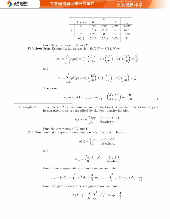
ii


ii

ii


xf(x, y) 0 1 2 h(y)

0 3/28 9/28 3/28 15/28

y 1 3/14 3/14 0 3/7

2 1/28 0 0 1/28

g(x) 5/14 15/28 3/28 1

Find the covariance of X and Y .Solution : From Example 2.28, we see that E(XY ) = 3/14. Now

µX =

2∑x=0

xg(x) = (0)

(5

14

)+ (1)

(15

28

)+ (2)

(3

28

)=

3

4,

and

µY =2∑

y=0

yh(y) = (0)

(15

28

)+ (1)

(3

7

)+ (2)

(1

28

)=

1

2.

Therefore,

σXY = E(XY )− µXµY =3

14−(3

4

)(1

2

)= − 9

56.

Example 2.36: The fraction X of male runners and the fraction Y of female runners who competein marathon races are described by the joint density function

f(x, y) =

{8xy, 0 ≤ y ≤ x ≤ 1,

0, elsewhere.

Find the covariance of X and Y .Solution : We first compute the marginal density functions. They are

g(x) =

{4x3, 0 ≤ x ≤ 1,

0, elsewhere,

and

h(y) =

{4y(1− y2), 0 ≤ y ≤ 1,

0, elsewhere.

From these marginal density functions, we compute

µX = E(X) =

∫ 1

0

4x4 dx =4

5and µY =

∫ 1

0

4y2(1− y2) dy =8

15.

From the joint density function given above, we have

E(XY ) =

∫ 1

0

∫ 1

y

8x2y2 dx dy =4

9.

ii


ii

ii


Then

σXY = E(XY )− µXµY =4

9−(4

5

)(8

15

)=

4

225.

Although the covariance between two random variables does provide informa-tion regarding the nature of the linear relationship, the magnitude of σXY doesnot indicate anything regarding the strength of the relationship, since σXY is notscale-free. Its magnitude will depend on the units used to measure both X and Y .There is a scale-free version of the covariance called the correlation coefficientthat is used widely in statistics.

Definition 2.18: Let X and Y be random variables with covariance σXY and standard deviationsσX and σY , respectively. The correlation coefficient of X and Y is

ρXY =σXY

σXσY

.

It should be clear to the reader that ρXY is free of the units of X and Y . Thecorrelation coefficient satisfies the inequality −1 ≤ ρXY ≤ 1. It assumes a value ofzero when σXY = 0. Where there is an exact linear dependency, say Y ≡ a+ bX,ρXY = 1 if b > 0 and ρXY = −1 if b < 0. (See Exercise 2.86.) The correlationcoefficient is the subject of more discussion in Chapter 7, where we deal with linearregression.

Example 2.37: Find the correlation coefficient between X and Y in Example 2.35.Solution : Since

E(X2) = (02)

(5

14

)+ (12)

(15

28

)+ (22)

(3

28

)=

27

28

and

E(Y 2) = (02)

(15

28

)+ (12)

(3

7

)+ (22)

(1

28

)=

4

7,

we obtain

σ2X =

27

28−(3

4

)2

=45

112and σ2

Y =4

7−(1

2

)2

=9

28.

Therefore, the correlation coefficient between X and Y is

ρXY =σXY

σXσY=

−9/56√(45/112)(9/28)

= − 1√5.

Example 2.38: Find the correlation coefficient of X and Y in Example 2.36.Solution : Because

E(X2) =

∫ 1

0

4x5 dx =2

3and E(Y 2) =

∫ 1

0

4y3(1− y2) dy = 1− 2

3=

1

3,

we conclude that

σ2X =

2

3−(4

5

)2

=2

75and σ2

Y =1

3−(

8

15

)2

=11

225.

ii


ii

ii


Hence,

ρXY =4/225√

(2/75)(11/225)=

4√66

.

Note that although the covariance in Example 2.37 is larger in magnitude (dis-regarding the sign) than that in Example 2.38, the relationship of the magnitudesof the correlation coefficients in these two examples is just the reverse. This isevidence that we cannot look at the magnitude of the covariance to decide on howstrong the relationship is.

Exercises

2.76 Use Definition 2.16 on page 82 to find the vari-ance of the random variable X of Exercise 2.55 on page79.

2.77 The random variable X, representing the num-ber of errors per 100 lines of software code, has thefollowing probability distribution:

x 2 3 4 5 6f(x) 0.01 0.25 0.4 0.3 0.04

Using Theorem 2.2 on page 83, find the variance of X.

2.78 Suppose that the probabilities are 0.4, 0.3, 0.2,and 0.1, respectively, that 0, 1, 2, or 3 power failureswill strike a certain subdivision in any given year. Findthe mean and variance of the random variable X repre-senting the number of power failures striking this sub-division.

2.79 A dealer’s profit, in units of $5000, on a newautomobile is a random variable X having the densityfunction given in Exercise 2.60 on page 80. Find thevariance of X.

2.80 The proportion of people who respond to a cer-tain mail-order solicitation is a random variable X hav-ing the density function given in Exercise 2.62 on page80. Find the variance of X.

2.81 The total number of hours, in units of 100 hours,that a family runs a vacuum cleaner over a period ofone year is a random variable X having the densityfunction given in Exercise 2.59 on page 79. Find thevariance of X.

2.82 Referring to Exercise 2.62 on page 80, find σ2g(X)

for the function g(X) = 3X2 + 4.

2.83 The length of time, in minutes, for an airplaneto obtain clearance for takeoff at a certain airport is arandom variable Y = 3X− 2, where X has the densityfunction

f(x) =

{14e−x/4, x > 0

0, elsewhere.

Find the mean and variance of the random variable Y .

2.84 Find the covariance of the random variables Xand Y of Exercise 2.36 on page 73.

2.85 For the random variables X and Y whose jointdensity function is given in Exercise 2.32 on page 72,find the covariance.

2.86 Given a random variable X, with standard de-viation σX , and a random variable Y = a + bX, showthat if b < 0, the correlation coefficient ρXY = −1, andif b > 0, ρXY = 1.

2.87 Consider the situation in Exercise 2.75 on page81. The distribution of the number of imperfectionsper 10 meters of synthetic fabric is given by

x 0 1 2 3 4f(x) 0.41 0.37 0.16 0.05 0.01

Find the variance and standard deviation of the num-ber of imperfections.

2.88 For a laboratory assignment, if the equipment isworking, the density function of the observed outcomeX is

f(x) =

{2(1− x), 0 < x < 1,

0, otherwise.

Find the variance and standard deviation of X.

2.89 For the random variables X and Y in Exercise2.31 on page 72, determine the correlation coefficientbetween X and Y .

2.90 Random variables X and Y follow a joint distri-bution

f(x, y) =

{2, 0 < x ≤ y < 1,

0, otherwise.

Determine the correlation coefficient between X andY .

ii


ii

ii

2.7 Means and Variances of Linear Combinations of Random Variables 89

2.7 Means and Variances of Linear Combinations ofRandom Variables

We now develop some useful properties that will simplify the calculations of meansand variances of random variables that appear in later chapters. These propertieswill permit us to deal with expectations in terms of other parameters that areeither known or easily computed. All the results that we present here are validfor both discrete and continuous random variables. Proofs are given only for thecontinuous case. We begin with a theorem and two corollaries that should be,intuitively, reasonable to the reader.

Theorem 2.5: If a and b are constants, then

E(aX + b) = aE(X) + b.

Proof : By the definition of expected value,

E(aX + b) =

∫ ∞

−∞(ax+ b)f(x) dx = a

∫ ∞

−∞xf(x) dx+ b

∫ ∞

−∞f(x) dx.

The first integral on the right is E(X) and the second integral equals 1. Therefore,we have

E(aX + b) = aE(X) + b.

Corollary 2.1: Setting a = 0, we see that E(b) = b.

Corollary 2.2: Setting b = 0, we see that E(aX) = aE(X).

Example 2.39: Applying Theorem 2.5 to the discrete random variable h(X) = 2X − 1, reworkExample 2.26 on page 77.

Solution : According to Theorem 2.5, we can write

E(2X − 1) = 2E(X)− 1.

Now

µ = E(X) =

9∑x=4

xf(x)

= (4)

(1

12

)+ (5)

(1

12

)+ (6)

(1

4

)+ (7)

(1

4

)+ (8)

(1

6

)+ (9)

(1

6

)=

41

6.

Therefore,

µ2X−1 = (2)

(41

6

)− 1 = $12.67,

as before.

ii


ii

ii


For the addition or subtraction of two functions of the random variable X, wehave the following theorem to compute its mean. The proof of the theorem is leftto the reader.

Theorem 2.6: The expected value of the sum or difference of two or more functions of a randomvariable X is the sum or difference of the expected values of the functions. Thatis,

E[g(X)± h(X)] = E[g(X)]± E[h(X)].

Example 2.40: Let X be a random variable with probability distribution as follows:x 0 1 2 3

f(x) 13

12 0 1

6

Find the expected value of Y = (X − 1)2.Solution : Applying Theorem 2.6 to the function Y = (X − 1)2, we can write

E[(X − 1)2] = E(X2 − 2X + 1) = E(X2)− 2E(X) + E(1).

From Corollary 2.1, E(1) = 1, and by direct computation,

E(X) = (0)

(1

3

)+ (1)

(1

2

)+ (2)(0) + (3)

(1

6

)= 1 and

E(X2) = (0)

(1

3

)+ (1)

(1

2

)+ (4)(0) + (9)

(1

6

)= 2.

Hence,

E[(X − 1)2] = 2− (2)(1) + 1 = 1.

Example 2.41: The weekly demand for a certain drink, in thousands of liters, at a chain ofconvenience stores is a continuous random variable g(X) = X2 +X − 2, where Xhas the density function

f(x) =

{2(x− 1), 1 < x < 2,

0, elsewhere.

Find the expected value of the weekly demand for the drink.Solution : By Theorem 2.6, we write

E(X2 +X − 2) = E(X2) + E(X)− E(2).

From Corollary 2.1, E(2) = 2, and by direct integration,

E(X) =

∫ 2

1

2x(x− 1) dx =5

3and E(X2) =

∫ 2

1

2x2(x− 1) dx =17

6.

Now

E(X2 +X − 2) =17

6+

5

3− 2 =

5

2,

ii


ii

ii


so the average weekly demand for the drink from this chain of efficiency stores is2500 liters.

Suppose that we have two random variables X and Y with joint probabilitydistribution f(x, y). Two additional properties that will be very useful in succeed-ing chapters involve the expected values of the sum, difference, and product ofthese two random variables. First, however, let us give a theorem on the expectedvalue of the sum or difference of functions of the given variables. This, of course, ismerely an extension of Theorem 2.6. The proof follows from the use of Definition2.15 and will be left to the reader.

Theorem 2.7: The expected value of the sum or difference of two or more functions of therandom variables X and Y is the sum or difference of the expected values of thefunctions. That is,

E[g(X,Y )± h(X,Y )] = E[g(X,Y )]± E[h(X,Y )].

Corollary 2.3: Setting g(X,Y ) = g(X) and h(X,Y ) = h(Y ), we see that

E[g(X)± h(Y )] = E[g(X)]± E[h(Y )].

Corollary 2.4: Setting g(X,Y ) = X and h(X,Y ) = Y , we see that

E[X ± Y ] = E[X]± E[Y ].

If X represents the daily production of some item from machine A and Y thedaily production of the same kind of item from machine B, then X +Y representsthe total number of items produced daily by both machines. Corollary 2.4 statesthat the average daily production for both machines is equal to the sum of theaverage daily production of each machine.

Theorem 2.8: Let X and Y be two independent random variables. Then

E(XY ) = E(X)E(Y ).

Proof : By Definition 2.15,

E(XY ) =

∫ ∞

−∞

∫ ∞

−∞xyf(x, y) dx dy.

Since X and Y are independent, we may write

f(x, y) = g(x)h(y),

where g(x) and h(y) are the marginal distributions ofX and Y , respectively. Hence,

E(XY ) =

∫ ∞

−∞

∫ ∞

−∞xyg(x)h(y) dx dy =

∫ ∞

−∞xg(x) dx

∫ ∞

−∞yh(y) dy

= E(X)E(Y ).

ii


ii

ii


Corollary 2.5: Let X and Y be two independent random variables. Then σXY = 0.

Proof : The proof can be carried out using Theorems 2.4 and 2.8, and Definition 2.14.

Example 2.42: It is known that the ratio of gallium to arsenide does not affect the functioningof gallium-arsenide wafers, which are the main components of some microchips.Let X denote the ratio of gallium to arsenide and Y denote the functional wafersretrieved during a 1-hour period. X and Y are independent random variables withthe joint density function

f(x, y) =

{x(1+3y2)

4 , 0 < x < 2, 0 < y < 1,

0, elsewhere.

Show that E(XY ) = E(X)E(Y ), as Theorem 2.8 suggests.Solution : By definition,

E(XY ) =

∫ 1

0

∫ 2

0

x2y(1 + 3y2)

4dx dy =

5

6, E(X) =

4

3, and E(Y ) =

5

8.

Hence,

E(X)E(Y ) =

(4

3

)(5

8

)=

5

6= E(XY ).

We conclude this section by proving one theorem and presenting several corol-laries that are useful for calculating variances or standard deviations.

Theorem 2.9: If X and Y are random variables with joint probability distribution f(x, y) anda, b, and c are constants, then

σ2aX+bY+c = a2σ2

X + b2σ2Y + 2abσXY .

Proof : By definition, σ2aX+bY+c = E{[(aX + bY + c)− µaX+bY+c]

2}. Now

µaX+bY+c = E(aX + bY + c) = aE(X) + bE(Y ) + c = aµX + bµY + c,

by using Corollary 2.4 followed by Corollary 2.2. Therefore,

σ2aX+bY+c = E{[a(X − µX) + b(Y − µY )]

2}= a2E[(X − µX)

2] + b2E[(Y − µY )2] + 2abE[(X − µX)(Y − µY )]

= a2σ2X + b2σ2

Y + 2abσXY .

Using Theorem 2.9, we have the following corollaries.

ii


ii

ii


Corollary 2.6: Setting b = 0, we see that

σ2aX+c = a2σ2

X = a2σ2.

Corollary 2.7: Setting a = 1 and b = 0, we see that

σ2X+c = σ2

X = σ2.

Corollary 2.8: Setting b = 0 and c = 0, we see that

σ2aX = a2σ2

X = a2σ2.

Corollaries 2.6 and 2.7 state that the variance is unchanged if a constant isadded to or subtracted from a random variable. The addition or subtraction ofa constant simply shifts the values of X to the right or to the left but does notchange their variability. However, if a random variable is multiplied or divided bya constant, then Corollaries 2.6 and 2.8 state that the variance is multiplied ordivided by the square of the constant.

Corollary 2.9: If X and Y are independent random variables, then

σ2aX+bY = a2σ2

X + b2σ2Y .

The result stated in Corollary 2.9 is obtained from Theorem 2.9 by invokingCorollary 2.5.

Corollary 2.10: If X and Y are independent random variables, then

σ2aX−bY = a2σ2

X + b2σ2Y .

Corollary 2.10 follows when b in Corollary 2.9 is replaced by −b. Generalizingto a linear combination of n independent random variables, we have Corollary 2.11.

Corollary 2.11: If X1, X2, . . . , Xn are independent random variables, then

σ2a1X1±a2X2±···±anXn

= a21σ2X1

+ a22σ2X2

+ · · ·+ a2nσ2Xn

.

Example 2.43: If X and Y are random variables with variances σ2X = 2 and σ2

Y = 4 and covarianceσXY = −2, find the variance of the random variable Z = 3X − 4Y + 8.

Solution :σ2Z = σ2

3X−4Y+8 = σ23X−4Y (by Corollary 2.6)

= 9σ2X + 16σ2

Y − 24σXY (by Theorem 2.9)

= (9)(2) + (16)(4)− (24)(−2) = 130.

ii


ii

ii


Example 2.44: Let X and Y denote the amounts of two different types of impurities in a batchof a certain chemical product. Suppose that X and Y are independent randomvariables with variances σ2

X = 2 and σ2Y = 3. Find the variance of the random

variable Z = 3X − 2Y + 5.Solution :

σ2Z = σ2

3X−2Y+5 = σ23X−2Y (by Corollary 2.6)

= 9σ2x + 4σ2

y (by Corollary 2.10)

= (9)(2) + (4)(3) = 30.

Exercises

2.91 Suppose that a grocery store purchases 5 car-tons of skim milk at the wholesale price of $1.20 percarton and retails the milk at $1.65 per carton. Afterthe expiration date, the unsold milk is removed fromthe shelf and the grocer receives a credit from the dis-tributor equal to three-fourths of the wholesale price.If the probability distribution of the random variableX, the number of cartons that are sold from this lot,is

x 0 1 2 3 4 5

f(x) 115

215

215

315

415

315

find the expected profit.

2.92 Repeat Exercise 2.83 on page 88 by applyingTheorem 2.5 and Corollary 2.6.

2.93 If a random variable X is defined such that

E[(X − 1)2] = 10 and E[(X − 2)2] = 6,

find µ and σ2.

2.94 The total time, measured in units of 100 hours,that a teenager runs her hair dryer over a period of oneyear is a continuous random variable X that has thedensity function

f(x) =

x, 0 < x < 1,

2− x, 1 ≤ x < 2,

0, elsewhere.

Use Theorem 2.6 to evaluate the mean of the randomvariable Y = 60X2 + 39X, where Y is equal to thenumber of kilowatt hours expended annually.

2.95 Use Theorem 2.7 to evaluate E(2XY 2 − X2Y )for the joint probability distribution shown in Table2.1 on page 64.

2.96 If X and Y are independent random variableswith variances σ2

X = 5 and σ2Y = 3, find the variance

of the random variable Z = −2X + 4Y − 3.

2.97 Repeat Exercise 2.96 if X and Y are not inde-pendent and σXY = 1.

2.98 Suppose that X and Y are independent randomvariables with probability densities and

g(x) =

{8x3 , x > 2,

0, elsewhere,

and

h(y) =

{2y, 0 < y < 1,

0, elsewhere.

Find the expected value of Z = XY .

2.99 Consider Review Exercise 2.117 on page 97. Therandom variables X and Y represent the number of ve-hicles that arrive at two separate street corners duringa certain 2-minute period in the day. The joint distri-bution is

f(x, y) =

(1

4(x+y)

)(9

16

),

for x = 0, 1, 2, . . . and y = 0, 1, 2, . . . .

(a) Give E(X), E(Y ), Var(X), and Var(Y ).

(b) Consider Z = X + Y , the sum of the two. FindE(Z) and Var(Z).

2.100 Consider Review Exercise 2.106 on page 95.There are two service lines. The random variables Xand Y are the proportions of time that line 1 and line2 are in use, respectively. The joint probability densityfunction for (X,Y ) is given by

f(x, y) =

{32(x2 + y2), 0 ≤ x, y ≤ 1,

0, elsewhere.

(a) Determine whether or not X and Y are indepen-dent.

ii


ii

ii

Review Exercises 95

(b) It is of interest to know something about the pro-portion of Z = X + Y , the sum of the two propor-tions. Find E(X + Y ). Also find E(XY ).

(c) Find Var(X), Var(Y ), and Cov(X,Y ).

(d) Find Var(X + Y ).

2.101 The length of time Y , in minutes, required togenerate a human reflex to tear gas has the densityfunction

f(y) =

{14e−y/4, 0 ≤ y < ∞,

0, elsewhere.

(a) What is the mean time to reflex?

(b) Find E(Y 2) and Var(Y ).

2.102 A manufacturing company has developed amachine for cleaning carpet that is fuel-efficient be-cause it delivers carpet cleaner so rapidly. Of inter-est is a random variable Y , the amount in gallons perminute delivered. It is known that the density functionis given by

f(y) =

{1, 7 ≤ y ≤ 8,

0, elsewhere.

(a) Sketch the density function.

(b) Give E(Y ), E(Y 2), and Var(Y ).

Review Exercises

2.103 A tobacco company produces blends of to-bacco, with each blend containing various proportionsof Turkish, domestic, and other tobaccos. The propor-tions of Turkish and domestic in a blend are randomvariables with joint density function (X = Turkish andY = domestic)

f(x, y) =

{24xy, 0 ≤ x, y ≤ 1, x+ y ≤ 1,

0, elsewhere.

(a) Find the probability that in a given box the Turkishtobacco accounts for over half the blend.

(b) Find the marginal density function for the propor-tion of the domestic tobacco.

(c) Find the probability that the proportion of Turk-ish tobacco is less than 1/8 if it is known that theblend contains 3/4 domestic tobacco.

2.104 An insurance company offers its policyholdersa number of different premium payment options. For arandomly selected policyholder, let X be the number ofmonths between successive payments. The cumulativedistribution function of X is

F (x) =

0, if x < 1,

0.4, if 1 ≤ x < 3,

0.6, if 3 ≤ x < 5,

0.8, if 5 ≤ x < 7,

1.0, if x ≥ 7.

(a) What is the probability mass function of X?

(b) Compute P (4 < X ≤ 7).

2.105 Two electronic components of a missile systemwork in harmony for the success of the total system.

Let X and Y denote the life in hours of the two com-ponents. The joint density of X and Y is

f(x, y) =

{ye−y(1+x), x, y ≥ 0,

0, elsewhere.

(a) Give the marginal density functions for both ran-dom variables.

(b) What is the probability that the lives of both com-ponents will exceed 2 hours?

2.106 A service facility operates with two servicelines. On a randomly selected day, let X be the pro-portion of time that the first line is in use whereas Yis the proportion of time that the second line is in use.Suppose that the joint probability density function for(X,Y ) is

f(x, y) =

{32(x2 + y2), 0 ≤ x, y ≤ 1,

0, elsewhere.

(a) Compute the probability that neither line is busymore than half the time.

(b) Find the probability that the first line is busy morethan 75% of the time.

2.107 Let the number of phone calls received by aswitchboard during a 5-minute interval be a randomvariable X with probability function

f(x) =e−22x

x!, for x = 0, 1, 2, . . . .

(a) Determine the probability that X equals 0, 1, 2, 3,4, 5, and 6.

(b) Graph the probability mass function for these val-ues of x.

ii


ii

ii


(c) Determine the cumulative distribution function forthese values of X.

2.108 An industrial process manufactures items thatcan be classified as either defective or not defective.The probability that an item is defective is 0.1. Anexperiment is conducted in which 5 items are drawnrandomly from the process. Let the random variable Xbe the number of defectives in this sample of 5. Whatis the probability mass function of X?

2.109 The life span in hours of an electrical compo-nent is a random variable with cumulative distributionfunction

F (x) =

{1− e−

x50 , x > 0,

0, eleswhere.

(a) Determine its probability density function.

(b) Determine the probability that the life span of sucha component will exceed 70 hours.

2.110 Pairs of pants are being produced by a particu-lar outlet facility. The pants are checked by a group of10 workers. The workers inspect pairs of pants takenrandomly from the production line. Each inspector isassigned a number from 1 through 10. A buyer selectsa pair of pants for purchase. Let the random variableX be the inspector number.

(a) Give a reasonable probability mass function for X.

(b) Plot the cumulative distribution function for X.

2.111 The shelf life of a product is a random variablethat is related to consumer acceptance. It turns outthat the shelf life Y in days of a certain type of bakeryproduct has a density function

f(y) =

{12e−y/2, 0 ≤ y < ∞,

0, elsewhere.

What fraction of the loaves of this product stocked to-day would you expect to be sellable 3 days from now?

2.112 Passenger congestion is a service problem inairports. Trains are installed within the airport to re-duce the congestion. With the use of the train, thetime X in minutes that it takes to travel from the mainterminal to a particular concourse has density function

f(x) =

{110, 0 ≤ x ≤ 10,

0, elsewhere.

(a) Show that the above is a valid probability densityfunction.

(b) Find the probability that the time it takes a pas-senger to travel from the main terminal to the con-course will not exceed 7 minutes.

2.113 Impurities in a batch of final product of achemical process often reflect a serious problem. Fromconsiderable plant data gathered, it is known that theproportion Y of impurities in a batch has a densityfunction given by

f(y) =

{10(1− y)9, 0 ≤ y ≤ 1,

0, elsewhere.

(a) Verify that the above is a valid density function.

(b) A batch is considered not sellable and then notacceptable if the percentage of impurities exceeds60%. With the current quality of the process, whatis the percentage of batches that are notacceptable?

2.114 The time Z in minutes between calls to an elec-trical supply system has the probability density func-tion

f(z) =

{110e−z/10, 0 < z < ∞,

0, elsewhere.

(a) What is the probability that there are no callswithin a 20-minute time interval?

(b) What is the probability that the first call comeswithin 10 minutes of opening?

2.115 A chemical system that results from a chemicalreaction has two important components among othersin a blend. The joint distribution describing the pro-portions X1 and X2 of these two components is givenby

f(x1, x2) =

{2, 0 < x1 < x2 < 1,

0, elsewhere.

(a) Give the marginal distribution of X1.

(b) Give the marginal distribution of X2.

(c) What is the probability that component propor-tions produce the results X1 < 0.2 and X2 > 0.5?

(d) Give the conditional distribution fX1|X2(x1|x2).

2.116 Consider the situation of Review Exercise2.115. But suppose the joint distribution of the twoproportions is given by

f(x1, x2) =

{6x2, 0 < x2 < x1 < 1,

0, elsewhere.

(a) Give the marginal distribution fX1(x1) of the pro-portion X1 and verify that it is a valid densityfunction.

(b) What is the probability that proportion X2 is lessthan 0.5, given that X1 is 0.7?

ii


ii

ii

Review Exercises 97

2.117 Consider the random variables X and Y thatrepresent the number of vehicles that arrive at two sep-arate street corners during a certain 2-minute period.These street corners are fairly close together so it is im-portant that traffic engineers deal with them jointly ifnecessary. The joint distribution of X and Y is knownto be

f(x, y) =9

16· 1

4(x+y),

for x = 0, 1, 2, . . . and y = 0, 1, 2, . . . .

(a) Are the two random variables X and Y indepen-dent? Explain why or why not.

(b) What is the probability that during the time pe-riod in question less than 4 vehicles arrive at thetwo street corners?

2.118 The behavior of series of components plays ahuge role in scientific and engineering reliability prob-lems. The reliability of the entire system is certainlyno better than that of the weakest component in theseries. In a series system, the components operate in-dependently of each other. In a particular system con-taining three components, the probabilities of meetingspecifications for components 1, 2, and 3, respectively,are 0.95, 0.99, and 0.92. What is the probability thatthe entire system works?

2.119 Another type of system that is employed in en-gineering work is a group of parallel components or aparallel system. In this more conservative approach,the probability that the system operates is larger thanthe probability that any component operates. The sys-tem fails only when all components fail. Consider a sit-uation in which there are 4 independent components ina parallel system with probability of operation given by

Component 1: 0.95; Component 2: 0.94;

Component 3: 0.90; Component 4: 0.97.

What is the probability that the system does not fail?

2.120 Consider a system of components in whichthere are 5 independent components, each of whichpossesses an operational probability of 0.92. The sys-tem does have a redundancy built in such that it doesnot fail if 3 out of the 5 components are operational.What is the probability that the total system is oper-ational?

2.121 Project: Take 5 class periods to observe theshoe color of individuals in class. Assume the shoecolor categories are red, white, black, brown, and other.Complete a frequency table for each color category.

(a) Estimate and interpret the meaning of the proba-bility distribution.

(b) What is the estimated probability that in the nextclass period a randomly selected student will bewearing a red or a white pair of shoes?

2.122 Referring to the random variables whose jointprobability density function is given in Exercise 2.38on page 73, find the average amount of kerosene left inthe tank at the end of the day.

2.123 Assume the length X, in minutes, of a particu-lar type of telephone conversation is a random variablewith probability density function

f(x) =

{15e−x/5, x > 0,

0, elsewhere.

(a) Determine the mean length E(X) of this type oftelephone conversation.

(b) Find the variance and standard deviation of X.

(c) Find E[(X + 5)2].

2.124 Suppose it is known that the life X of a par-ticular compressor, in hours, has the density function

f(x) =

{1

900e−x/900, x > 0,

0, elsewhere.

(a) Find the mean life of the compressor.

(b) Find E(X2).

(c) Find the variance and standard deviation of therandom variable X.

2.125 Referring to the random variables whose jointdensity function is given in Exercise 2.32 on page 72,

(a) find µX and µY ;

(b) find E[(X + Y )/2].

2.126 Show that Cov(aX, bY ) = ab Cov(X,Y ).

2.127 Consider Exercise 2.58 on page 79. Can it besaid that the ratings given by the two experts are in-dependent? Explain why or why not.

2.128 A company’s marketing and accounting de-partments have determined that if the company mar-kets its newly developed product, the contribution ofthe product to the firm’s profit during the next 6months will be described by the following:

Profit Contribution Probability

−$5, 000$10, 000$30, 000

0.20.50.3

What is the company’s expected profit?

ii


ii

ii


2.129 In a support system in the U.S. space program,a single crucial component works only 85% of the time.In order to enhance the reliability of the system, it isdecided that 3 components will be installed in parallelsuch that the system fails only if they all fail. Assumethe components act independently and that they areequivalent in the sense that all 3 of them have an 85%success rate. Consider the random variable X as thenumber of components out of 3 that fail.

(a) Write out a probability function for the randomvariable X.

(b) What is E(X) (i.e., the mean number of compo-nents out of 3 that fail)?

(c) What is Var(X)?

(d) What is the probability that the entire system issuccessful?

(e) What is the probability that the system fails?

(f) If the desire is to have the system be successfulwith probability 0.99, are three components suffi-cient? If not, how many are required?

2.130 It is known through data collection and con-siderable research that the amount of time in secondsthat a certain employee of a company is late for workis a random variable X with density function

f(x) =

{3

(4)(503)(502 − x2), −50 ≤ x ≤ 50,

0, elsewhere.

In other words, he not only is slightly late at times,but also can be early to work.

(a) Find the expected value of the time in seconds thathe is late.

(b) Find E(X2).

(c) What is the standard deviation of the amount oftime he is late?

2.131 A delivery truck travels from point A to pointB and back using the same route each day. There arefour traffic lights on the route. Let X1 denote the num-ber of red lights the truck encounters going from A toB and X2 denote the number encountered on the re-turn trip. Data collected over a long period suggestthat the joint probability distribution for (X1, X2) isgiven by

x2

x1 0 1 2 3 4

0 0.01 0.01 0.03 0.07 0.011 0.03 0.05 0.08 0.03 0.022 0.03 0.11 0.15 0.01 0.013 0.02 0.07 0.10 0.03 0.014 0.01 0.06 0.03 0.01 0.01

(a) Give the marginal density of X1.

(b) Give the marginal density of X2.

(c) Give the conditional density distribution of X1

given X2 = 3.

(d) Give E(X1).

(e) Give E(X2).

(f) Give E(X1 | X2 = 3).

(g) Give the standard deviation of X1.

2.132 A convenience store has two separate locationswhere customers can be checked out as they leave.These locations each have two cash registers and twoemployees who check out customers. Let X be thenumber of cash registers being used at a particular timefor location 1 and Y the number being used at the sametime for location 2. The joint probability function isgiven by

y

x 0 1 2

0 0.12 0.04 0.041 0.08 0.19 0.052 0.06 0.12 0.30

(a) Give the marginal density of both X and Y as wellas the probability distribution of X given Y = 2.

(b) Give E(X) and Var(X).

(c) Give E(X | Y = 2) and Var(X | Y = 2).

2.133 As we shall illustrate in Chapter 7, statisticalmethods associated with linear and nonlinear modelsare very important. In fact, exponential functions areoften used in a wide variety of scientific and engineeringproblems. Consider a model that is fit to a set of datainvolving measured values k1 and k2 and a certain re-sponse Y to the measurements. The model postulatedis

Y = eb0+b1k1+b2k2 ,

where Y denotes the estimated value of Y, k1 andk2 are fixed values, and b0, b1, and b2 are estimatesof constants and hence are random variables. Assumethat these random variables are independent and usethe approximate formula for the variance of a nonlinearfunction of more than one variable. Give an expression

for Var(Y ). Assume that the means of b0, b1, and b2are known and are β0, β1, and β2, and assume that thevariances of b0, b1, and b2 are known and are σ2

0 , σ21 ,

and σ22 .

2.134 Consider Review Exercise 2.113 on page 96. Itinvolved Y , the proportion of impurities in a batch,and the density function is given by

f(y) =

{10(1− y)9, 0 ≤ y ≤ 1,

0, elsewhere.

ii


ii

ii

2.8 Potential Misconceptions and Hazards 99

(a) Find the expected percentage of impurities.

(b) Find the expected value of the proportion of qualitymaterial (i.e., find E(1− Y )).

(c) Find the variance of the random variable Z = 1−Y .

2.135 Project: Let X = number of hours each stu-dent in the class slept the night before. Create a dis-crete variable by using the following arbitrary intervals:X < 3, 3 ≤ X < 6, 6 ≤ X < 9, and X ≥ 9.

(a) Estimate the probability distribution for X.

(b) Calculate the estimated mean and variance for X.

2.8 Potential Misconceptions and Hazards;Relationship to Material in Other Chapters

The material in this chapter is extremely fundamental in nature. We focused ongeneral characteristics of a probability distribution and defined important quanti-ties or parameters that characterize the general nature of the system. The mean ofa distribution reflects central tendency, and the variance or standard deviationreflects variability in the system. In addition, covariance reflects the tendency fortwo random variables to “move together” in a system. These important parameterswill remain fundamental to all that follows in this text.

The reader should understand that the distribution type is often dictated bythe scientific scenario. However, the parameter values often need to be estimatedfrom scientific data. For example, in the case of Review Exercise 2.124, the manu-facturer of the compressor may know (material that will be presented in Chapter3) from experience and knowledge of the type of compressor that the nature of thedistribution is as indicated in the exercise. The mean µ would not be known butestimated from experimentation on the machine. Though the parameter value of900 is given as known here, it will not be known in real-life situations without theuse of experimental data.

ii


ii

ii

Documents

Random Variables, Distributions, and Expectations