Discrete Random Variables & Distributions

stat 430Heike Hofmann

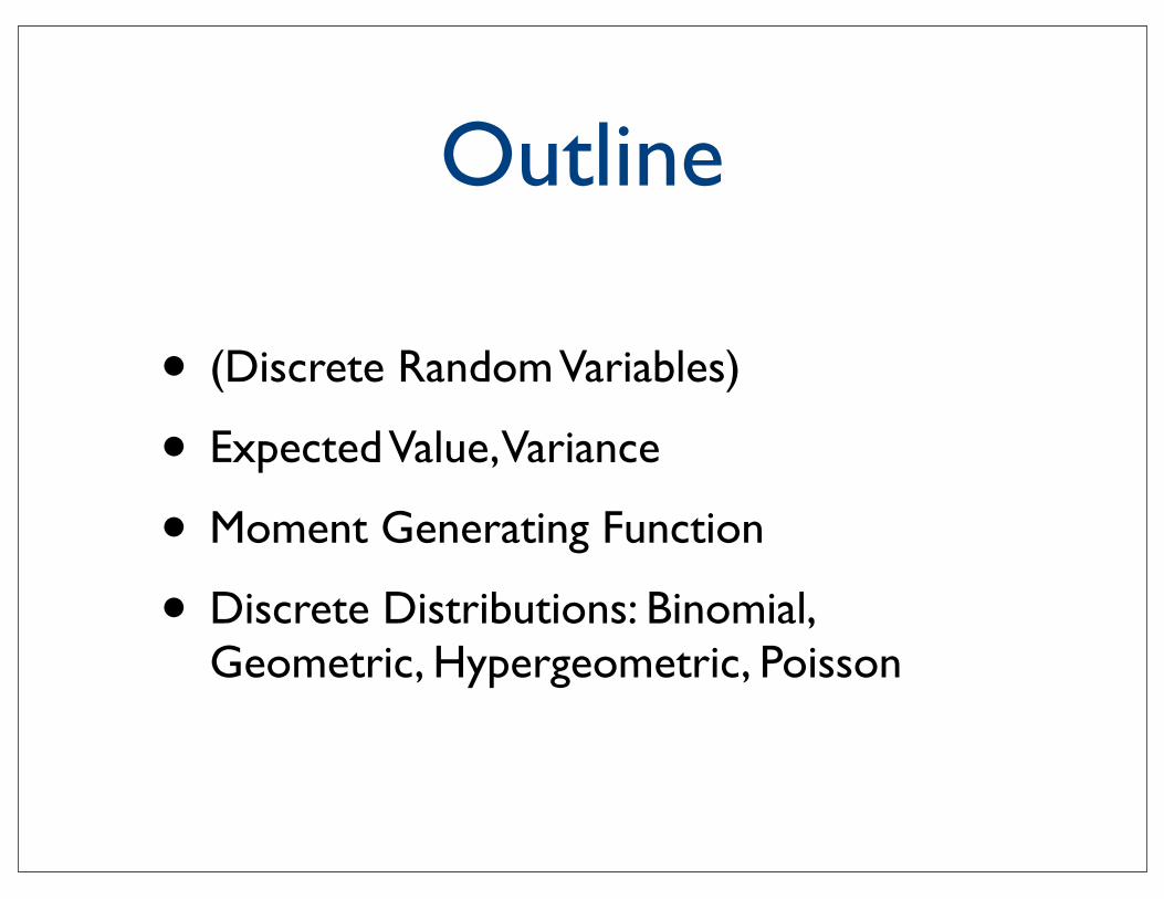
Outline

• (Discrete Random Variables)

• Expected Value, Variance

• Moment Generating Function

• Discrete Distributions: Binomial, Geometric, Hypergeometric, Poisson

V ar[X] =

i

(xi − E[X])2 · pX(xi)

The function pX(x) := P (X = x) is called the probability mass function of X. Aprobability mass function has two main properties: Properties of a pmf pX is the pmf ofX, if and only if

(i) all values must be between 0 and 1 0 ≤ pX(x) ≤ 1 for all x ∈ x1, x2, x3, . . .

(ii) the sum of all values is 1

i pX(xi) = 1

E[h(X)] =

i

h(xi) · pX(xi) =: µ

Ωk = 00...00, 00...01, 00...10, 00...11,

...,

11...00, 11...01, 11...10, 11...11

A function X : Ω → R is called a random variable.

k

i

P (X = k) =

n

k

pk(1− p)n−k

(i) 0 ≤ P (A) ≤ 1

(ii) P (∅) = 0

(iii) for pairwise disjoint events A1, A2, A3, ...

P (A1 ∪A2 ∪A3 ∪ ...) = P (A1) + P (A2) + P (A3) + ...

P (Ω) = 1

P (A) = 1− P (A)

P (A ∪B) = P (A) + P (B)− P (A ∩B)

Ω1 =

(1, 1), (1, 2) ... (1, 6)(2, 1), (2, 2) ... (2, 6)

......

. . ....

(6, 1), (6, 2) ... (6, 6)

5

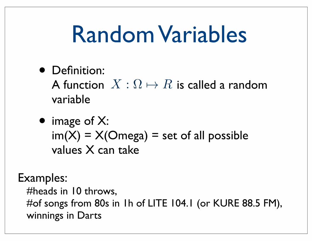
Random Variables• Definition:

A function is called a random variable

• image of X: im(X) = X(Omega) = set of all possible values X can take

Examples: #heads in 10 throws, #of songs from 80s in 1h of LITE 104.1 (or KURE 88.5 FM), winnings in Darts

V ar[X] =

i

(xi − E[X])2 · pX(xi)

The function pX(x) := P (X = x) is called the probability mass function of X. Aprobability mass function has two main properties: Properties of a pmf pX is the pmf ofX, if and only if

(i) all values must be between 0 and 1 0 ≤ pX(x) ≤ 1 for all x ∈ x1, x2, x3, . . .

(ii) the sum of all values is 1

i pX(xi) = 1

E[h(X)] =

i

h(xi) · pX(xi) =: µ

Ωk = 00...00, 00...01, 00...10, 00...11,

...,

11...00, 11...01, 11...10, 11...11

A function X : Ω → R is called a random variable.

k

i

P (X = k) =

n

k

pk(1− p)n−k

(i) 0 ≤ P (A) ≤ 1

(ii) P (∅) = 0

(iii) for pairwise disjoint events A1, A2, A3, ...

P (A1 ∪A2 ∪A3 ∪ ...) = P (A1) + P (A2) + P (A3) + ...

P (Ω) = 1

P (A) = 1− P (A)

P (A ∪B) = P (A) + P (B)− P (A ∩B)

Ω1 =

(1, 1), (1, 2) ... (1, 6)(2, 1), (2, 2) ... (2, 6)

......

. . ....

(6, 1), (6, 2) ... (6, 6)

5

V ar[X] =

i

(xi − E[X])2 · pX(xi)

The function pX(x) := P (X = x) is called the probability mass function of X. Aprobability mass function has two main properties: Properties of a pmf pX is the pmf ofX, if and only if

(i) all values must be between 0 and 1 0 ≤ pX(x) ≤ 1 for all x ∈ x1, x2, x3, . . .

(ii) the sum of all values is 1

i pX(xi) = 1

E[h(X)] =

i

h(xi) · pX(xi) =: µ

Ωk = 00...00, 00...01, 00...10, 00...11,

...,

11...00, 11...01, 11...10, 11...11

A function X : Ω → R is called a random variable.

k

i

P (X = k) =

n

k

pk(1− p)n−k

(i) 0 ≤ P (A) ≤ 1

(ii) P (∅) = 0

(iii) for pairwise disjoint events A1, A2, A3, ...

P (A1 ∪A2 ∪A3 ∪ ...) = P (A1) + P (A2) + P (A3) + ...

P (Ω) = 1

P (A) = 1− P (A)

P (A ∪B) = P (A) + P (B)− P (A ∩B)

Ω1 =

(1, 1), (1, 2) ... (1, 6)(2, 1), (2, 2) ... (2, 6)

......

. . ....

(6, 1), (6, 2) ... (6, 6)

5

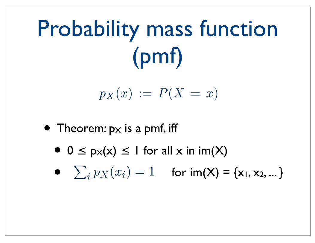
Probability mass function (pmf)

• Theorem: pX is a pmf, iff

• 0 ≤ pX(x) ≤ 1 for all x in im(X)

• for im(X) = x1, x2, ...

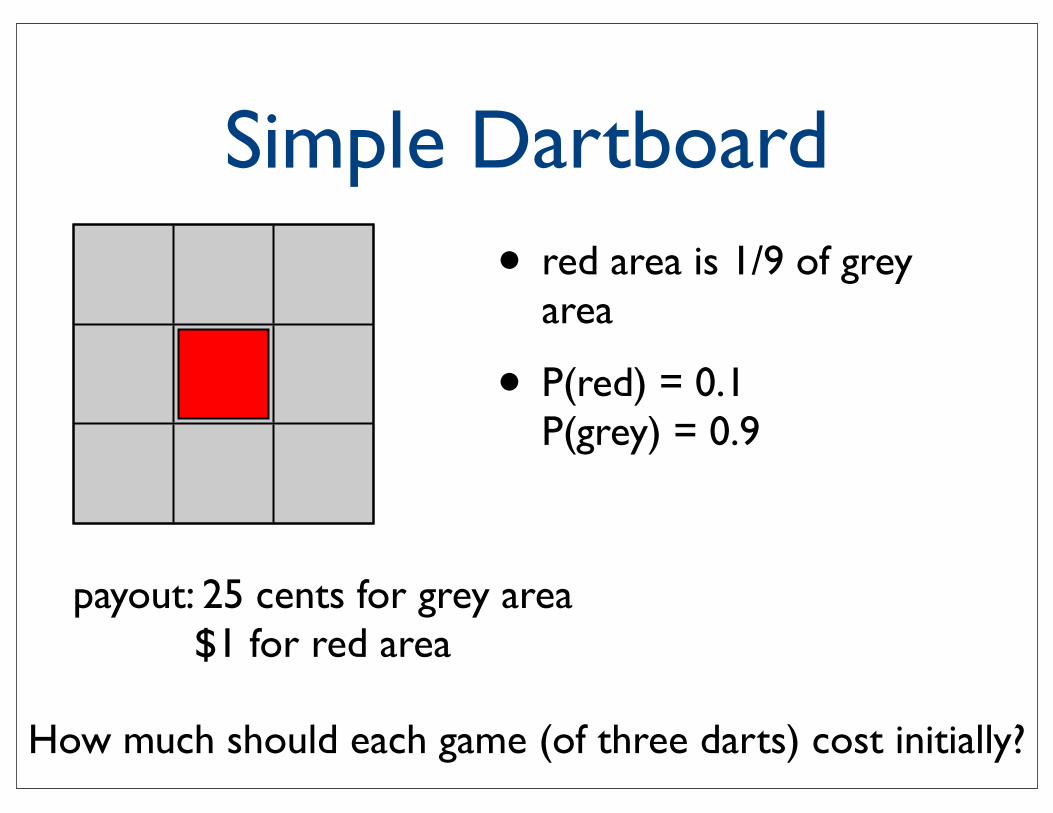
Simple Dartboard• red area is 1/9 of grey

area

• P(red) = 0.1P(grey) = 0.9

payout: 25 cents for grey area$1 for red area

How much should each game (of three darts) cost initially?

Expectation

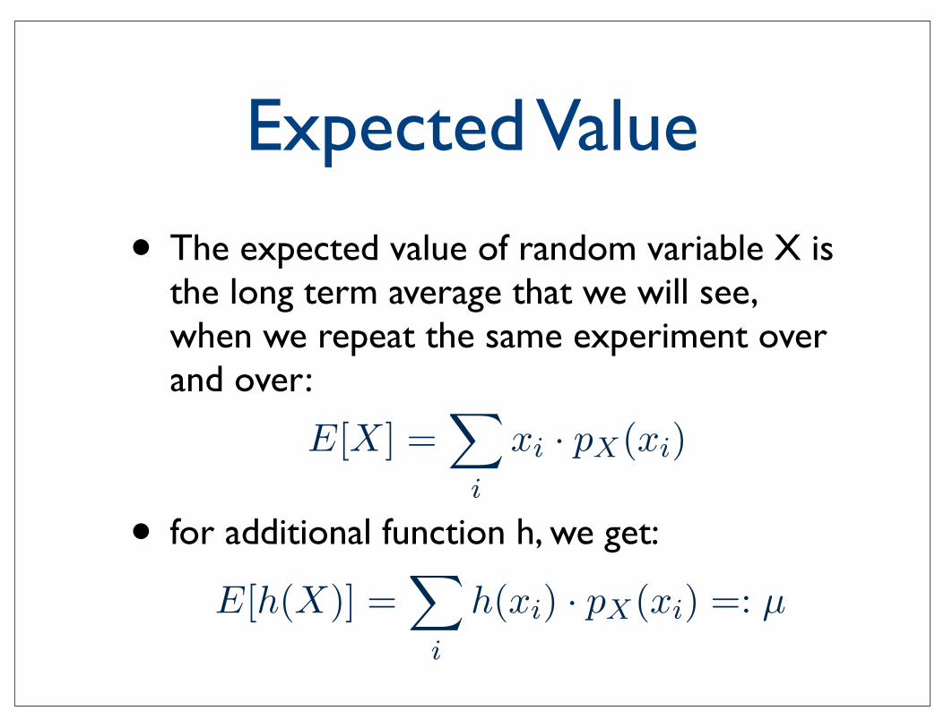
Expected Value

• The expected value of random variable X is the long term average that we will see, when we repeat the same experiment over and over:

• for additional function h, we get:

V ar[X] =

i

(xi − E[X])2 · pX(xi)

The function pX(x) := P (X = x) is called the probability mass function of X. Aprobability mass function has two main properties: Properties of a pmf pX is the pmf ofX, if and only if

(i) all values must be between 0 and 1 0 ≤ pX(x) ≤ 1 for all x ∈ x1, x2, x3, . . .

(ii) the sum of all values is 1

i pX(xi) = 1

E[h(X)] =

i

h(xi) · pX(xi) =: µ

Ωk = 00...00, 00...01, 00...10, 00...11,

...,

11...00, 11...01, 11...10, 11...11

A function X : Ω → R is called a random variable.

k

i

P (X = k) =

n

k

pk(1− p)n−k

(i) 0 ≤ P (A) ≤ 1

(ii) P (∅) = 0

(iii) for pairwise disjoint events A1, A2, A3, ...

P (A1 ∪A2 ∪A3 ∪ ...) = P (A1) + P (A2) + P (A3) + ...

P (Ω) = 1

P (A) = 1− P (A)

P (A ∪B) = P (A) + P (B)− P (A ∩B)

Ω1 =

(1, 1), (1, 2) ... (1, 6)(2, 1), (2, 2) ... (2, 6)

......

. . ....

(6, 1), (6, 2) ... (6, 6)

5

V ar[X] =

i

(xi − E[X])2 · pX(xi)

The function pX(x) := P (X = x) is called the probability mass function of X. Aprobability mass function has two main properties: Properties of a pmf pX is the pmf ofX, if and only if

(i) all values must be between 0 and 1 0 ≤ pX(x) ≤ 1 for all x ∈ x1, x2, x3, . . .

(ii) the sum of all values is 1

i pX(xi) = 1

E[h(X)] =

i

h(xi) · pX(xi) =: µ

E[X] =

i

xi · pX(xi) =: µ

Ωk = 00...00, 00...01, 00...10, 00...11,

...,

11...00, 11...01, 11...10, 11...11

A function X : Ω → R is called a random variable.

k

i

P (X = k) =

n

k

pk(1− p)n−k

(i) 0 ≤ P (A) ≤ 1

(ii) P (∅) = 0

(iii) for pairwise disjoint events A1, A2, A3, ...

P (A1 ∪A2 ∪A3 ∪ ...) = P (A1) + P (A2) + P (A3) + ...

P (Ω) = 1

P (A) = 1− P (A)

P (A ∪B) = P (A) + P (B)− P (A ∩B)

5

Variance

V ar[X] =

i

(xi − E[X])2 · pX(xi)

The function pX(x) := P (X = x) is called the probability mass function of X. Aprobability mass function has two main properties: Properties of a pmf pX is the pmf ofX, if and only if

(i) all values must be between 0 and 1 0 ≤ pX(x) ≤ 1 for all x ∈ x1, x2, x3, . . .

(ii) the sum of all values is 1

i pX(xi) = 1

E[h(X)] =

i

h(xi) · pX(xi) =: µ

E[X] =

i

xi · pX(xi) =: µ

Ωk = 00...00, 00...01, 00...10, 00...11,

...,

11...00, 11...01, 11...10, 11...11

A function X : Ω → R is called a random variable.

k

i

P (X = k) =

n

k

pk(1− p)n−k

(i) 0 ≤ P (A) ≤ 1

(ii) P (∅) = 0

(iii) for pairwise disjoint events A1, A2, A3, ...

P (A1 ∪A2 ∪A3 ∪ ...) = P (A1) + P (A2) + P (A3) + ...

P (Ω) = 1

P (A) = 1− P (A)

P (A ∪B) = P (A) + P (B)− P (A ∩B)

5

Variance

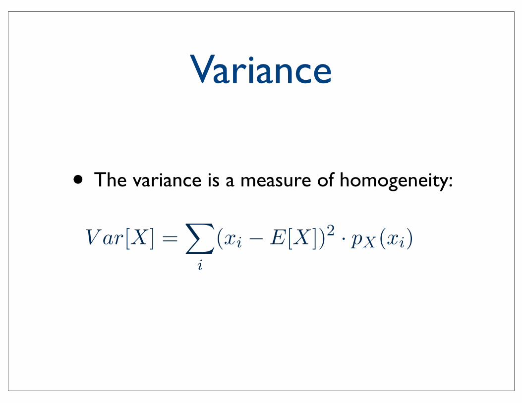
• The variance is a measure of homogeneity:

Rules for E[X] and Var[X]

• Let X and Y be two random variables, and a,b two real values, then

• E[aX+bY] = a E[X] + b E[Y]E[XY] = E[X]E[Y], if X, Y are independent

• Var[X] = E[X2] - (E[X])2

• Var[aX] = a2 Var[X]Var[X+Y] = Var[X] + Var[Y], if X,Y are ind.

Moment Generating Function

discrete random variable continuous random variableimage Im(X) finite or countable infinite image Im(X) uncountable

probability distribution function:

FX(t) = P (X ≤ t) =

k≤t pX(k) FX(t) = P (X ≤ t) = t∞ f(x)dx

probability mass function:pX(x) = P (X = x)

probability density function:fX(x) = F

X(x)

expected value:E[h(X)] =

x h(x) · pX(x) E[h(X)] =

x h(x) · fX(x)

variance:V ar[X] = E[(X − E[X])2] =

x(x −

E[X])2pX(x)V ar[X] = E[(X − E[X])2] =

=

∞

−∞(x− E[X])2fX(x)dx

ρ :=Cov(X,Y )

V ar(X) · V ar(Y )

read: “rho” Facts about ρ:

• ρ is between -1 and 1

• if ρ = 1 or -1, Y is a linear function of X

ρ = 1 → Y = aX + b with a > 0,ρ = −1 → Y = aX + b with a < 0,

ρ is a measure of linear association between X and Y . ρ near ±1 indicates a strong linearrelationship, ρ near 0 indicates lack of linear association.

E[h(X,Y )] :=

x,y

h(x, y)pX,Y (x, y)

Cov(X,Y ) = E[(X − E[X])(Y − E[Y ])]

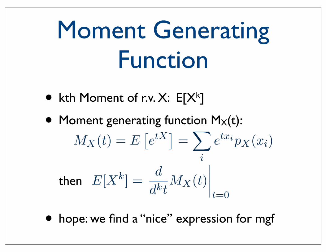
E[Xk] =d

dktMX(t)

t=0

MX(t) = EetX

=

i

etxipX(xi)

4

discrete random variable continuous random variableimage Im(X) finite or countable infinite image Im(X) uncountable

probability distribution function:

FX(t) = P (X ≤ t) =

k≤t pX(k) FX(t) = P (X ≤ t) = t∞ f(x)dx

probability mass function:pX(x) = P (X = x)

probability density function:fX(x) = F

X(x)

expected value:E[h(X)] =

x h(x) · pX(x) E[h(X)] =

x h(x) · fX(x)

variance:V ar[X] = E[(X − E[X])2] =

x(x −

E[X])2pX(x)V ar[X] = E[(X − E[X])2] =

=

∞

−∞(x− E[X])2fX(x)dx

ρ :=Cov(X,Y )

V ar(X) · V ar(Y )

read: “rho” Facts about ρ:

• ρ is between -1 and 1

• if ρ = 1 or -1, Y is a linear function of X

ρ = 1 → Y = aX + b with a > 0,ρ = −1 → Y = aX + b with a < 0,

ρ is a measure of linear association between X and Y . ρ near ±1 indicates a strong linearrelationship, ρ near 0 indicates lack of linear association.

E[h(X,Y )] :=

x,y

h(x, y)pX,Y (x, y)

Cov(X,Y ) = E[(X − E[X])(Y − E[Y ])]

E[Xk] =d

dktMX(t)

t=0

MX(t) = EetX

=

i

etxipX(xi)

4

Moment Generating Function

• kth Moment of r.v. X: E[Xk]

• Moment generating function MX(t):

then

• hope: we find a “nice” expression for mgf

Special Distributions

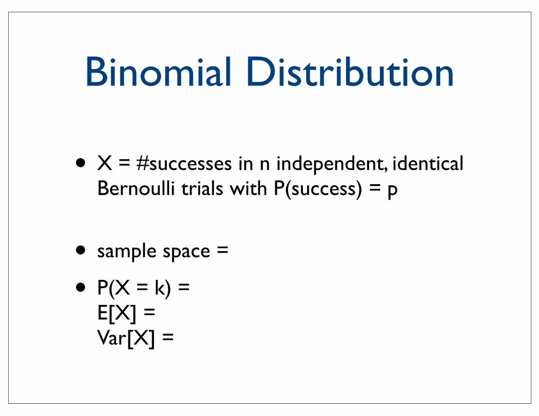
Binomial Distribution

• X = #successes in n independent, identical Bernoulli trials with P(success) = p

• sample space =

• P(X = k) = E[X] = Var[X] =

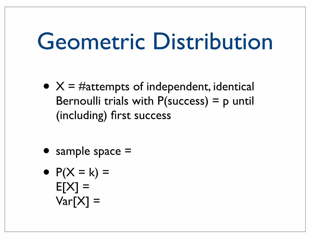
Geometric Distribution

• X = #attempts of independent, identical Bernoulli trials with P(success) = p until (including) first success

• sample space =

• P(X = k) = E[X] = Var[X] =

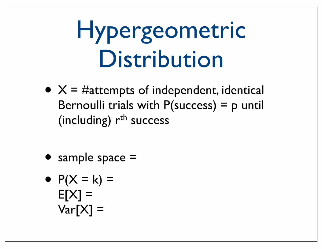
Hypergeometric Distribution

• X = #attempts of independent, identical Bernoulli trials with P(success) = p until (including) rth success

• sample space =

• P(X = k) = E[X] = Var[X] =

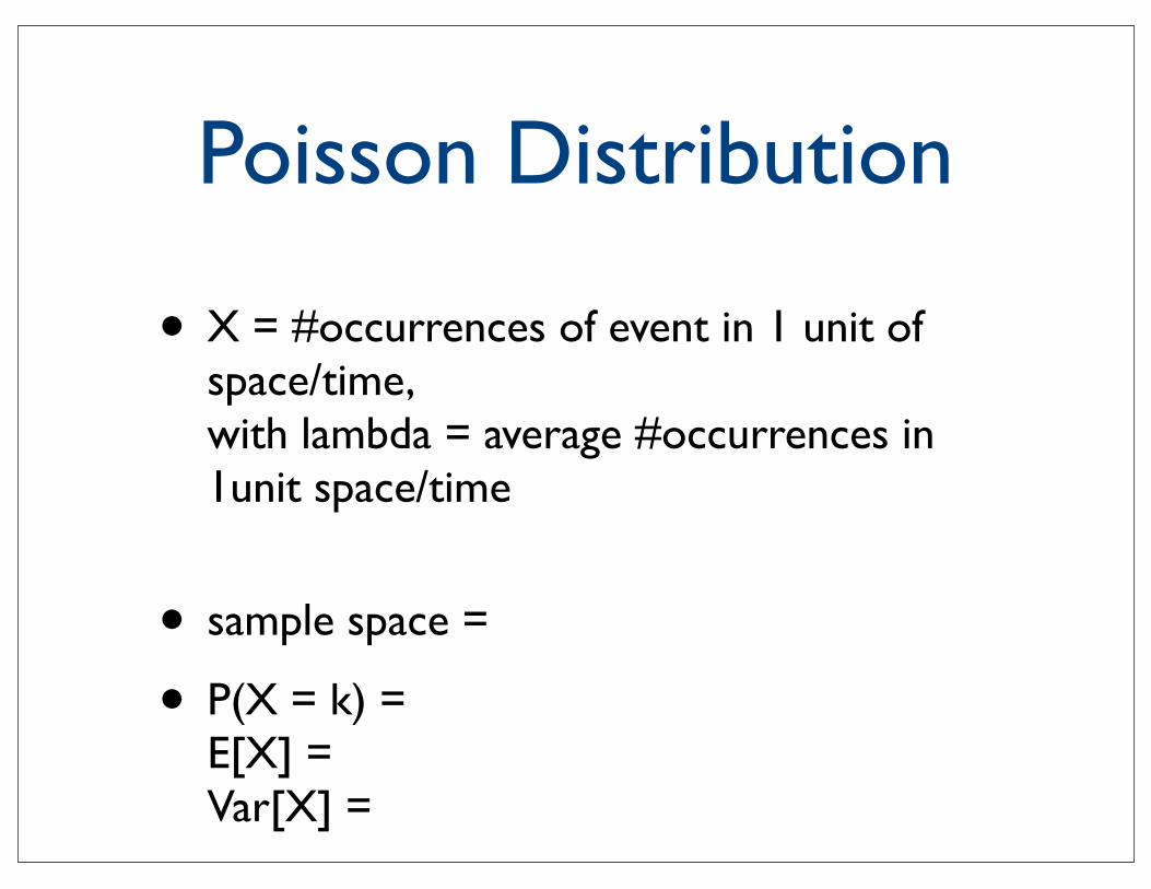
Poisson Distribution

• X = #occurrences of event in 1 unit of space/time,with lambda = average #occurrences in 1unit space/time

• sample space =

• P(X = k) = E[X] = Var[X] =

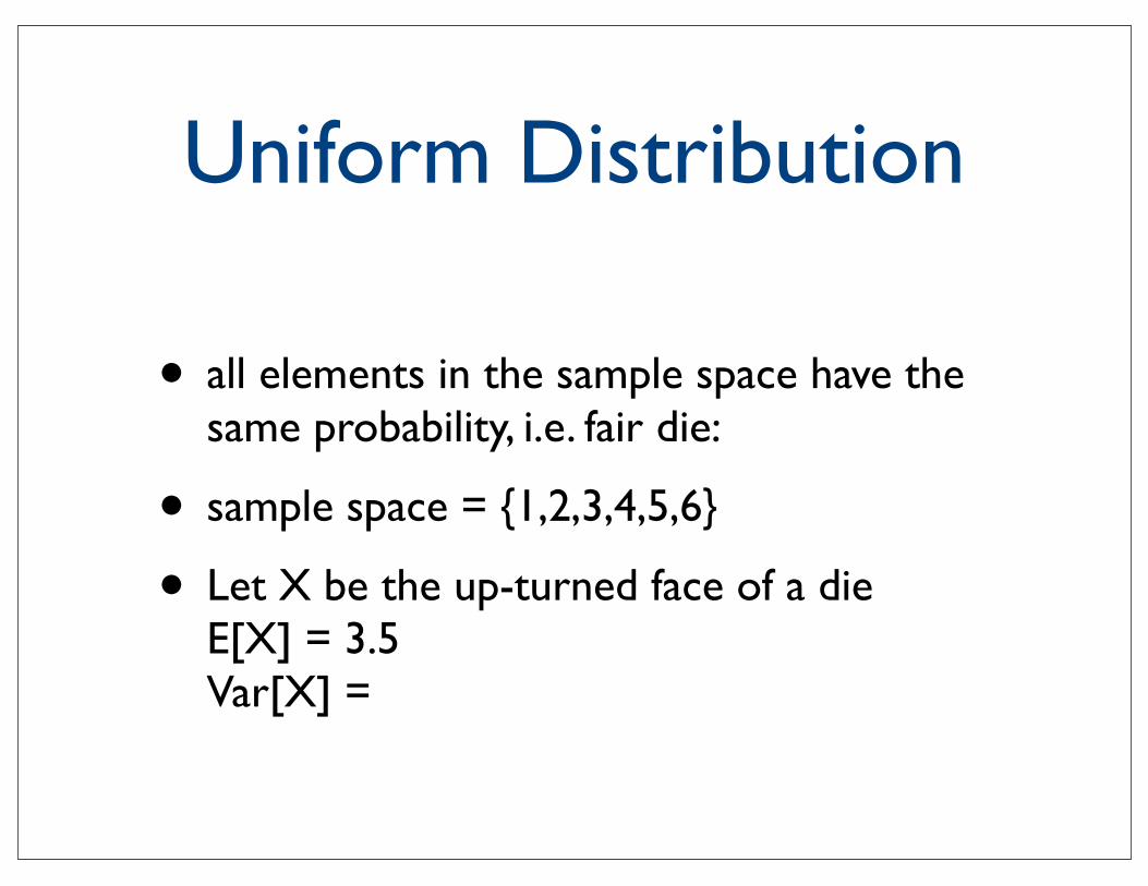
Uniform Distribution

• all elements in the sample space have the same probability, i.e. fair die:

• sample space = 1,2,3,4,5,6

• Let X be the up-turned face of a dieE[X] = 3.5Var[X] =