Embed Size (px)
Citation preview
1
Random Regret-based discrete choice modeling:
A tutorial
Caspar Chorus
Section of Transport and Logistics / Department of Infrastructure Systems and Services /
Faculty of Technology, Policy and Management / Delft University of Technology
Jaffalaan 5, 2628BX, Delft, The Netherlands, T: +31152788546, E: [email protected]
Version: February 20th
, 2012
Please cite as:
Chorus CG (2012) Random Regret-based discrete choice modeling: A tutorial. Springer, Heidelberg, Germany

2
3
Abstract
This tutorial presents a hands-on introduction to a new discrete choice modeling approach based on the
behavioral notion of regret-minimization. This so-called Random Regret Minimization-approach (RRM)
forms a counterpart of the Nobel prize winning Random Utility Maximization-approach (RUM) to
discrete choice modeling, which has for decades dominated the field of choice modeling and adjacent
fields such as transportation, marketing and environmental economics. Being as parsimonious as
conventional RUM-models and compatible with popular software packages, the RRM-approach provides
an alternative and appealing account of choice behavior. A variety of empirically well-established
behavioral phenomena that are not captured by conventional RUM-models readily emerge from the
RRM-model’s structure in a way that is consistent with the model’s underlying behavioral premises.
Since its introduction in 2010, the RRM-approach has been used by a growing number of leading choice
modelers in a variety of decision-making contexts, showing a promising potential in terms of model fit
and predictive ability.
Rather than providing highly technical discussions as usually encountered in scholarly journals covering
discrete choice models, this tutorial aims to allow readers to explore the RRM-approach and its potential
and limitations hands-on and based on a detailed discussion of examples. This tutorial is written for
students, scholars and practitioners who have a basic background in choice modeling in general and
RUM-modeling in particular. It has been taken care of that all concepts and results should be clear to
readers that do not have an advanced knowledge of econometrics.
Following a brief introduction, Chapter 2 presents the RRM-approach to discrete choice modeling.
Comparisons with the RUM-based Multinomial Logit-model are provided where relevant. In Chapter 3,
the focus is on how to estimate RRM-models and how to interpret estimation results and use them for
forecasting – the Chapter discusses data-requirements and software issues, and presents an empirical
example in-depth. In Chapter 4, the general applicability of the RRM-model is discussed, and its strong
points and limitations are highlighted. Chapter 5 presents a selection of recent developments in RRM-
modeling.

4
5
Contents
1. Introduction .......................................................................................................................................... 7
2. A Random Regret Minimization-based discrete choice model ........................................................... 11
2.1. A Random Regret-function .......................................................................................................... 11
2.2. A comparison with (linear-additive) utility maximization ........................................................... 16
2.3. Regret-based choice probabilities and a RRM-based MNL-model .............................................. 21
3. Empirical application of Random Regret Minimization-models ......................................................... 25
3.1. The data ...................................................................................................................................... 25
3.2 Model estimation ........................................................................................................................ 27
3.3. Model fit ...................................................................................................................................... 30
3.4. Interpretation of parameters ...................................................................................................... 32
3.5. Market share forecasting ............................................................................................................ 40
3.6. Out-of-sample validity................................................................................................................. 45
4. Applicability of Random Regret Minimization-models , and their strong and weak points .............. 47
4.1. General applicability ................................................................................................................... 47
4.1.1. Non-generic attributes ........................................................................................................ 47
4.1.2. Constants ............................................................................................................................ 48
4.1.3. Non-continuous (categorical) attributes ............................................................................. 49
4.1.4. Hybrid RUM-RRM models ................................................................................................... 50
4.1.5. Interactions with socio-demographic variables .................................................................. 50
4.2. RRM: strong points...................................................................................................................... 51
4.3. RRM: weak points ....................................................................................................................... 52
5. Selection of recent developments in RRM-modeling ......................................................................... 55
5.1. Random regret minimization for decision-making under uncertainty ........................................ 55
5.2 RRM for modeling household or group decision-making ............................................................ 58
5.3 The expected regret of a choice-situation: An RRM-based Logsum ........................................... 61
5.4 An RRM-based formulation of ‘Value of Time’ ........................................................................... 64
References .................................................................................................................................................. 67
Appendix: Investigating the assumption of i.i.d. errors in RRM-models ............................................. 69

6
7
1. Introduction
Since their inception in the 1970s (McFadden 1974), Discrete Choice Models (DCMs from here on) have
been used to explain choice-behavior of individuals and predict market shares for products and services
in a wide variety of contexts. Numerous studies worldwide have been performed over the years to
provide quantitative analyses and forecasts of choice behavior and market shares in fields as diverse as
transportation, health care, consumer choice, and environmental economics – to name a few. DCMs use
observed choices between different options (for example: stated or revealed choices between different
travel modes on a given route) to derive the underlying preferences of individuals. When one has
information about the characteristics of the different choice options – such as the travel times and costs
of the different travel modes – DCMs make it possible to estimate the weights that decision-makers
attach to these different characteristics when making decisions. Knowing these weights is valuable in
itself. However, they can also be put to use to predict the effect on market shares of, say, an increase in
bus-fare of a particular magnitude. This ability of DCMs to provide quantitative estimates of decision-
makers’ preferences, and of the market shares that are the aggregate result of these preferences, has
made them very popular among scholars and practitioners alike.
Basically, each DCM is defined in terms of a combination of an assumed decision rule and an assumed
error term structure. The error terms that enter DCMs represent the fact that the researcher cannot
‘look into the heads’ of decision-makers, so that part of what drives their choice-behavior remains
unobserved. Lately, the DCM-field has seen numerous innovations in error term specifications, allowing
for an ever more realistic representation of the unobserved part of behavior. This tutorial will not pay
much attention to these developments; note that excellent textbooks exist that cover them in much
detail (e.g., Train 2003). Instead, the tutorial will mainly focus on the decision rule assumed in DCMs.
In terms of the assumed decision-rule, DCMs, like every model, present a simplified version of reality:
although it is well known that choice-behavior may be the result of numerous interrelated processes
and impulses, a DCM must reduce this complexity to a great extent in order to be of practical use. One
of the ways in which DCMs reduce the complexity of actual behavior is by assuming a relatively
straightforward decision-rule which translates decision makers’ preferences and tastes (e.g., a dislike of
long travel times), in combination with the characteristics of choice-options (e.g., a bus service’s travel
time), into predicted choice patterns (e.g., a particular bus service’s market share on a given route).
8
More specifically, the overwhelming majority of DCMs are based on a so-called utility maximization-
based decision rule. This decision rule postulates that when choosing between different options,
decision makers attach a utility to each option and choose the one that has the highest utility. Apart
from an error term, this utility usually consists of a linear-additive function of characteristics of the
choice-option and associated parameters (the latter represent decision weights associated with these
characteristics). DCMs that are based on such utility maximization-based decision rules are called
Random Utility Maximization-models (the term ‘Random’ stands for the error term that is added). This
utilitarian category of DCMs (from here on: RUM-models or RUM-based DCMs1) has been by far the
most used DCM since its inception, earning the main developer (Daniel McFadden) a Nobel Prize. The
popularity of RUM-models both in- and outside academia is a direct result of their tractability, ease of
use and solid foundation in microeconomic axioms.
Notwithstanding this popularity of the utility-based modeling approach, interest in the incorporation of
alternative decision rules in DCMs has existed for as long as RUM-models have. This tutorial focuses on
such a non-utilitarian DCM called Random Regret Minimization or RRM, which has been recently
proposed by the author of this tutorial (Chorus 2010)2. This regret-based DCM-approach is based on the
notion that when choosing, people anticipate and aim to minimize regret rather than maximize utility.
Regret arises when one or more non-chosen alternatives perform better than the chosen one in terms
of one or more attributes. The notion that people are regret-minimizers has been very well established
empirically in a variety of fields (e.g., Zeelenberg & Pieters 2007), but the translation of this behavioral
notion in an operational DCM that enables the econometric analysis of multi-attribute alternatives in
multi-alternative choice sets is recent. RRM distinguishes itself from other extensions of and alternatives
for RUM-models by presenting a tractable, parsimonious model form that is easily estimable using
standard software packages. In other words: the model consumes no more parameters than
conventional (linear-additive) RUM-based DCMs, and it is user-friendly. Notwithstanding that the model
1 Unless explicitly stated otherwise, a reference to RUM-models in this tutorial implies a reference to linear-
additive RUM-based multinomial logit (or MNL) models as presented in section 2.2.
2 Note that an earlier version of the RRM-model has been presented in (Chorus et al. 2008). However, the RRM-
model form presented in that paper featured a non-smooth likelihood-function which hampered the model’s
applicability and usability (for example: it relied on handwritten code). This manual focuses on a more recent
model form, published in 2010 (Chorus 2010); this latter model form features a smooth likelihood-function and can
be estimated using standard software-packages.
9
has only been introduced very recently, it has already been successfully applied by a rapidly growing
number of researchers from a variety of leading research groups worldwide3. Applications include but
are not limited to travelers’ choices between destinations, travel modes, routes, departure times,
parking lots, and travel information services; tourists’ choices between recreational activities; patients’
choices between medical treatments; consumers’ choices between vehicle-types; politicians’ choices
between policy-options; and singles’ choices between on-line dating profiles.
Motivated by the growing popularity of RRM-based DCMs, this tutorial aims to provide an introduction
to regret-based choice modeling for students and practitioners, as well as for scholars with a basic
understanding of discrete choice-modeling and an interest in RRM. In contrast with published scholarly
papers on RRM, whose main aim is to communicate new research findings to fellow discrete choice-
modelers, the tutorial has an educational purpose. It aims to help the reader (i) understand the RRM-
approach to discrete choice modeling (ii) appreciate how RRM-models differ from RUM-models
conceptually and operationally, (iii) understand how the RRM-model can be used in practice to analyze
choice-data, and (iv) appreciate its potential and limitations. Although equations are presented
wherever relevant, the manual is written in a way that facilitates understanding of RRM-models and
their properties also for readers that have only moderate experience in working with mathematical
formulations. However, a working knowledge of discrete choice modeling in general and the RUM-based
MNL-model is required, as is a basic understanding of stated choice-data collection methods4. The
majority of examples used is obtained from the field of transportation in general and travel behavior in
particular. However, applicability of derivations, results and discussions in other fields than
transportation will be obvious and intuitive.
Chapter 2 presents the RRM-approach to discrete choice modeling. Comparisons with the RUM-based
MNL-model are provided where relevant. In Chapter 3, the focus is on how to estimate RRM-models and
how to use estimation results for forecasting – it discusses data-requirements, software issues and
presents an empirical example in-depth. In Chapter 4, the general applicability of the RRM-model is
3 See Chorus (2012) for a recent overview of empirical applications.
4 See Ben-Akiva & Lerman (1985) and Train (2003) for examples of textbooks that provide excellent introductions
to discrete choice-modeling and RUM’s MNL-model (besides offering much material for more advanced choice-
modelers as well). Hensher et al. (2005) provide an excellent introduction to stated choice methods, as well as
much material at a more advanced level.
10
discussed, and its strong points and limitations are discussed. Chapter 5 presents a selection of recent
developments in RRM-modeling.
I would like to thank Eric Molin for reading and commenting an earlier version of the first four chapters
of this tutorial. Furthermore, I have had many very fruitful discussions about RRM with a variety of
choice modelers, especially with people with whom I have been or currently am doing research and
writing papers on this topic: Jan Anne Annema, Theo Arentze, Richard Batley, Matthew Beck, Shlomo
Bekhor, Esther de Bekker-Grob, Michel Bierlaire, Michiel Bliemer, Marco Boeri, Bill Greene, David
Hensher, Stephane Hess, Anco Hoen, Gerard de Jong, Mark Koetse, Niek Mouter, John Nellthorp, John
Rose, Ric Scarpa, Mara Thiene, Harry Timmermans, Tomer Toledo, and Bert van Wee. Discussions with
these scholars have no doubt refined my own thinking on RRM, and I would like to thank them for that.
Support from the Netherlands Organization for Scientific Research (NWO), in the form of VENI-grant
451-10-001, is gratefully acknowledged.
11
2. A Random Regret Minimization-based discrete choice model
This Chapter presents the RRM-model. First, the Random Regret function is presented and explained
(Section 2.1). Subsequently, this function is compared with the classical linear-additive Random Utility-
function (Section 2.2). Finally, it is shown how the Random Regret-function translates into MNL-type
choice probabilities for a particular distribution of the random error terms (Section 2.3).
2.1. A Random Regret-function
The key behavioral notion on which the RRM-model is built is that people, when choosing, compare a
considered alternative with each of the other available alternatives in terms of each characteristic (or
from here on: attribute), and that they wish to avoid the situation where a chosen alternative is
outperformed by one or more other alternatives on one or more attributes (which would cause regret)5.
Importantly, in contrast with other models and theories that are based on regret-minimization, the
RRM-model postulates that anticipated regret is also a determinant of choices when there is no
uncertainty about the performance of alternatives. The RRM-model postulates that as long as
alternatives are characterized in terms of multiple attributes, which implies that trade-offs have to be
made by the decision-maker, there will be regret in the sense that there will generally be at least one
non-chosen alternative that outperforms a chosen one in terms of one or more attributes.
More specifically, the RRM-model is designed to incorporate the following seven behavioral intuitions
relating to the anticipated regret associated with a considered alternative:
5 Obviously, the level of anticipated regret that is associated with a particular alternative will vary between
individuals. More specifically, different individuals may have different tastes and perceptions regarding
alternatives and their attributes. Mathematically, this heterogeneity across individuals can be expressed by making
relevant terms in the regret equation presented below (such as � and �) individual-specific by means of an index
(usually ‘n’). In this tutorial, for reasons of readability, no such indices are used. As a result, equations refer to (the
tastes and perceptions of) an average or ‘representative’ individual.
12
1. when a considered alternative outperforms another alternative in terms of a particular attribute, the
comparison of the considered alternative with the other alternative on that attribute does not
generate anticipated regret.
2. when a considered alternative is outperformed by another alternative in terms of a particular
attribute, the comparison of the considered alternative with the other alternative on that attribute
generates anticipated regret.
3. anticipated regret increases with the importance of the attribute on which a considered alternative
is outperformed by another alternative.
4. anticipated regret increases with the magnitude of the extent to which a considered alternative is
outperformed by another alternative on a particular attribute.
5. anticipated regret increases with the number of attributes on which the considered alternative is
outperformed by another alternative.
6. anticipated regret increases with the number of alternatives that outperform a considered one on a
particular attribute.
7. anticipated regret is, from the perspective of the analyst, partially ‘observable’ (in the sense that it
can be explicitly linked to observed variables) and partially ‘unobservable’.
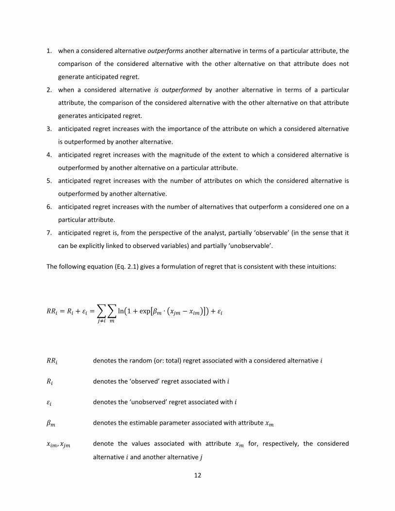
The following equation (Eq. 2.1) gives a formulation of regret that is consistent with these intuitions:
��� � �� � �� ���ln1 � exp��� ∙ ��� � ���������� � ��
��� denotes the random (or: total) regret associated with a considered alternative � �� denotes the ‘observed’ regret associated with � �� denotes the ‘unobserved’ regret associated with � �� denotes the estimable parameter associated with attribute ��
���, ��� denote the values associated with attribute �� for, respectively, the considered
alternative � and another alternative�
13
Before discussing this function in more depth, it should be noted that of course, constants can be added
to regret-functions, to represent the mean unobserved regrets associated with particular alternatives.
Also, note that attributes may take the form of continuous variables as well as variables of categorical
measurement level. Furthermore note that socio-demographic variables (such as age, gender, income
and education level) may enter the regret-function to express segmentations of the population in terms
of preferences for alternatives and tastes for attributes. Finally, note that in this chapter the focus is on
attributes that are common, or shared, or generic, across alternatives. See chapter 4 for an in-depth
discussion of how the RRM-model deals with constants, interactions with socio-demographic variables,
non-continuous variables, and with attributes that are specific to particular alternatives.
Returning to the regret-equation presented above: the term ln1 � exp��� ∙ ��� � ������ is the core
of this equation: it forms a measure of the amount of regret that is associated with comparing a
considered alternative � with another alternative� in terms of a particular attribute ��. This attribute-
level regret is computed for each of the bilateral comparisons with other alternatives, and for all
available attributes; the summation of these attribute-level regret terms (totaling � * (� – 1) terms in a
situation where there are � attributes and the choice set contains � alternatives) forms the observed
regret that is associated with the considered alternative. In light of the important role of attribute-level
regret, also when it comes to deriving and interpreting the properties of the RRM-model, it is worth
paying additional attention to this regret-kernel.
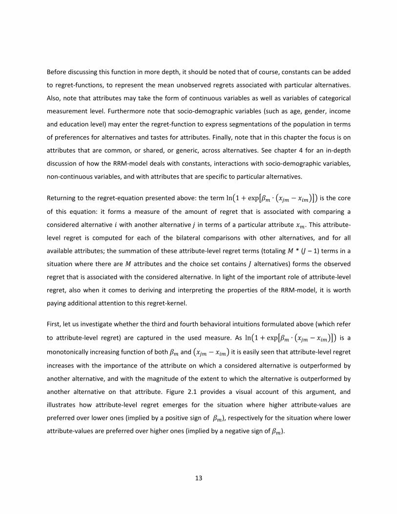
First, let us investigate whether the third and fourth behavioral intuitions formulated above (which refer
to attribute-level regret) are captured in the used measure. As ln1 � exp��� ∙ ��� � ������ is a
monotonically increasing function of both �� and ��� � ���� it is easily seen that attribute-level regret
increases with the importance of the attribute on which a considered alternative is outperformed by
another alternative, and with the magnitude of the extent to which the alternative is outperformed by
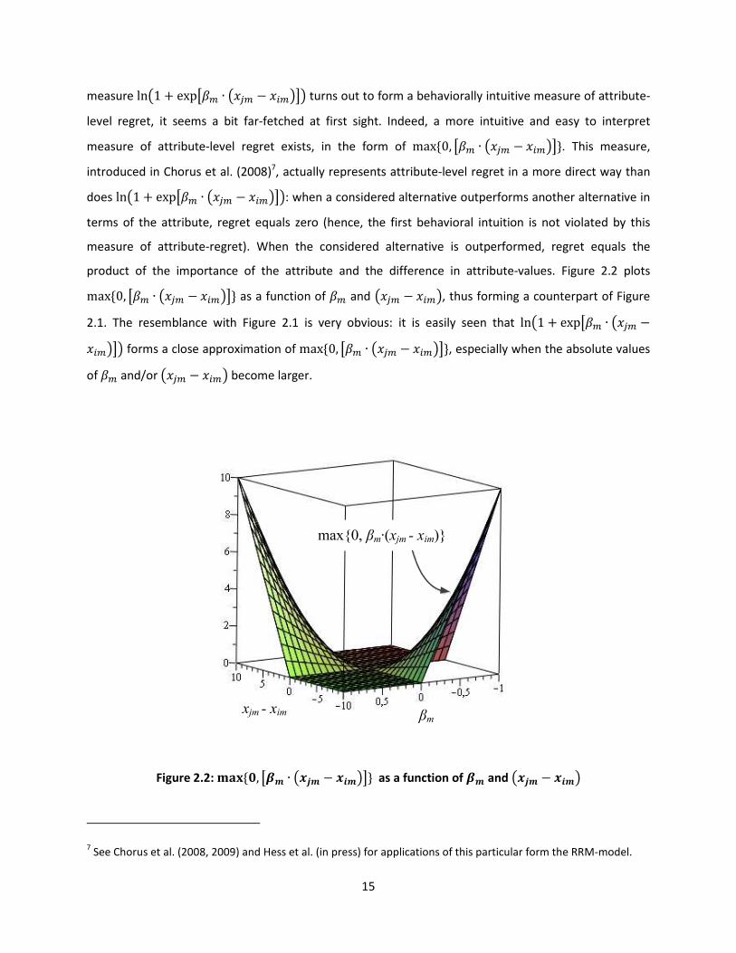
another alternative on that attribute. Figure 2.1 provides a visual account of this argument, and
illustrates how attribute-level regret emerges for the situation where higher attribute-values are
preferred over lower ones (implied by a positive sign of ��), respectively for the situation where lower
attribute-values are preferred over higher ones (implied by a negative sign of ��).
14
xjm - xim βm
ln(1+exp[βm·(xjm - xim)])
Figure 2.1: Attribute-level regret as a function of �� and !� � "��
More specifically, when higher attribute-values are preferred over lower ones, regret emerges to the
extent that ��� becomes larger than ��� and to the extent that �� becomes more positive. In contrast,
when lower attribute-values are preferred over higher ones, regret emerges to the extent that ���
becomes smaller than ��� and to the extent that �� becomes more negative. When the product �� ∙ ��� � ���� becomes negative (i.e., when the considered alternative outperforms the other
alternative with which it is compared in terms of the attribute), attribute-regret starts to approach zero6.
Note that strictly speaking, the fact that attribute-regret approaches rather than equals zero when the
considered alternative outperforms the other alternative implies that the first of the seven behavioral
intuitions formulated at the beginning of this Chapter is violated. More generally speaking, although the
6 It should be noted at this point that during the estimation process the sign of parameters is estimated together
with their magnitude. That is, no a priori expectations need to be formulated by the analyst in terms of whether
higher attribute-values are preferred by the decision-maker over lower ones, or vice versa.
15
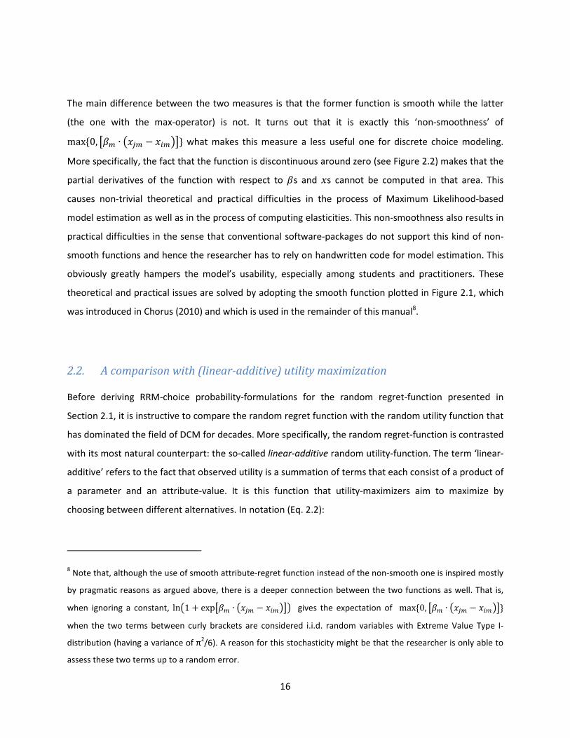
measure ln1 � exp��� ∙ ��� � ������ turns out to form a behaviorally intuitive measure of attribute-
level regret, it seems a bit far-fetched at first sight. Indeed, a more intuitive and easy to interpret
measure of attribute-level regret exists, in the form of max%0, ��� ∙ ��� � �����'. This measure,
introduced in Chorus et al. (2008)7, actually represents attribute-level regret in a more direct way than
does ln1 � exp��� ∙ ��� � ������: when a considered alternative outperforms another alternative in
terms of the attribute, regret equals zero (hence, the first behavioral intuition is not violated by this
measure of attribute-regret). When the considered alternative is outperformed, regret equals the
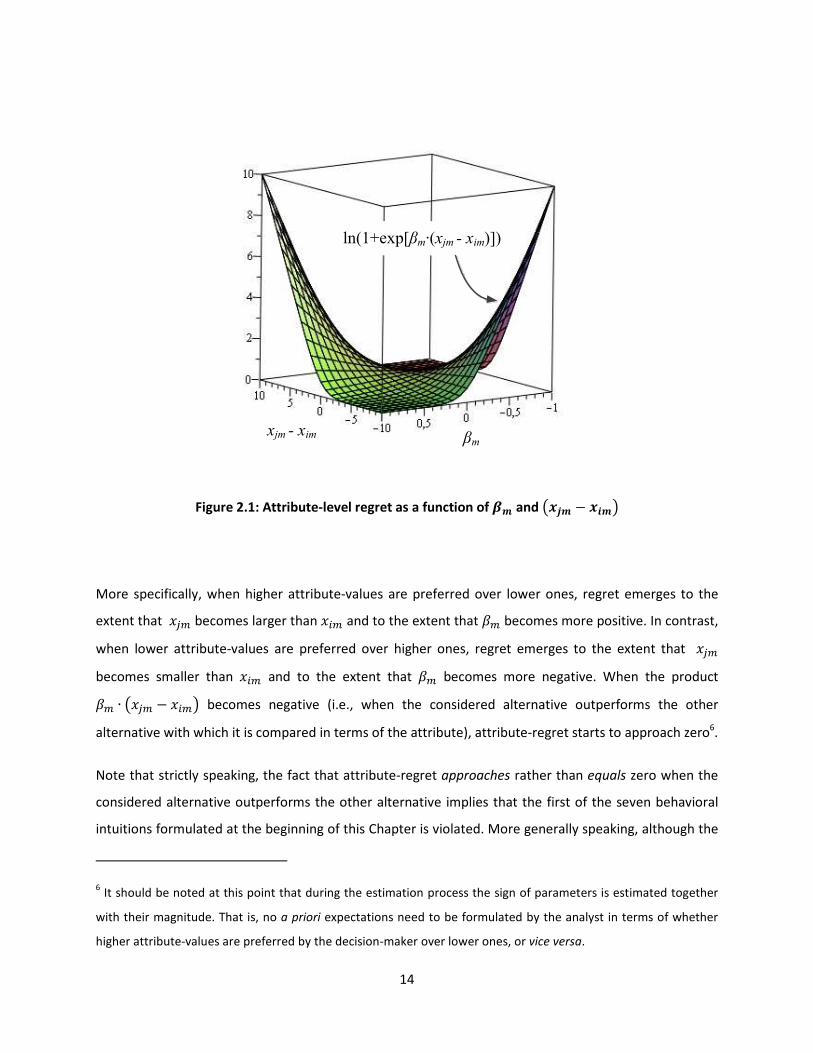
product of the importance of the attribute and the difference in attribute-values. Figure 2.2 plots max%0, ��� ∙ ��� � �����' as a function of �� and ��� � ����, thus forming a counterpart of Figure
2.1. The resemblance with Figure 2.1 is very obvious: it is easily seen that ln1 � exp��� ∙ ��� ������� forms a close approximation of max%0, ��� ∙ ��� � �����', especially when the absolute values
of �� and/or ��� � ���� become larger.
xjm - xim βm
max{0, βm·(xjm - xim)}
Figure 2.2: ()*%+, ��� ∙ !� � "���' as a function of �� and !� � "��
7 See Chorus et al. (2008, 2009) and Hess et al. (in press) for applications of this particular form the RRM-model.
16
The main difference between the two measures is that the former function is smooth while the latter
(the one with the max-operator) is not. It turns out that it is exactly this ‘non-smoothness’ of max%0, ��� ∙ ��� � �����' what makes this measure a less useful one for discrete choice modeling.
More specifically, the fact that the function is discontinuous around zero (see Figure 2.2) makes that the
partial derivatives of the function with respect to �s and �s cannot be computed in that area. This
causes non-trivial theoretical and practical difficulties in the process of Maximum Likelihood-based
model estimation as well as in the process of computing elasticities. This non-smoothness also results in
practical difficulties in the sense that conventional software-packages do not support this kind of non-
smooth functions and hence the researcher has to rely on handwritten code for model estimation. This
obviously greatly hampers the model’s usability, especially among students and practitioners. These
theoretical and practical issues are solved by adopting the smooth function plotted in Figure 2.1, which
was introduced in Chorus (2010) and which is used in the remainder of this manual8.
2.2. A comparison with (linear-additive) utility maximization
Before deriving RRM-choice probability-formulations for the random regret-function presented in
Section 2.1, it is instructive to compare the random regret function with the random utility function that
has dominated the field of DCM for decades. More specifically, the random regret-function is contrasted
with its most natural counterpart: the so-called linear-additive random utility-function. The term ‘linear-
additive’ refers to the fact that observed utility is a summation of terms that each consist of a product of
a parameter and an attribute-value. It is this function that utility-maximizers aim to maximize by
choosing between different alternatives. In notation (Eq. 2.2):
8 Note that, although the use of smooth attribute-regret function instead of the non-smooth one is inspired mostly
by pragmatic reasons as argued above, there is a deeper connection between the two functions as well. That is,
when ignoring a constant, ln1 � exp��� ∙ ��� � ������ gives the expectation of max%0, ��� ∙ ��� � �����' when the two terms between curly brackets are considered i.i.d. random variables with Extreme Value Type I-
distribution (having a variance of π2/6). A reason for this stochasticity might be that the researcher is only able to
assess these two terms up to a random error.
17
,� � -� � �� ���� ∙� ��� � ��
,� denotes the random (or: total) utility associated with a considered alternative � -� denotes the ‘observed’ utility associated with � �� denotes the ‘unobserved’ utility associated with � �� denotes the estimable parameter associated with attribute ��
��� denotes the value associated with attribute �� for the considered alternative �
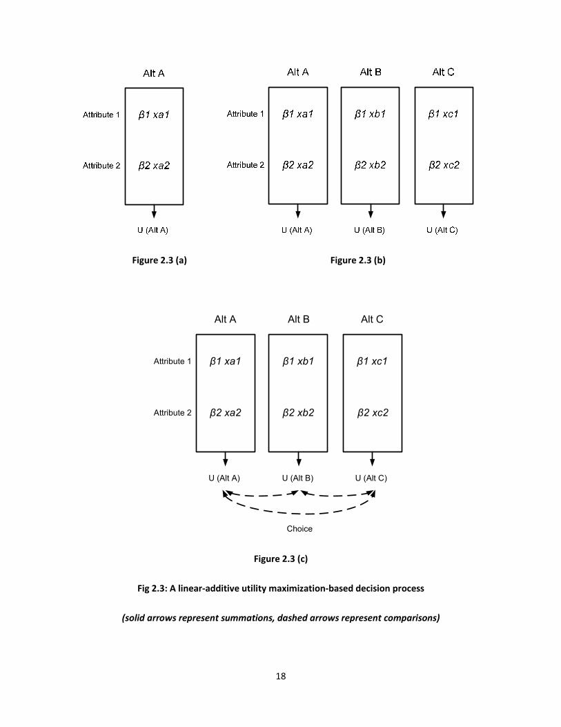
The conceptual differences between the utility-function presented directly above and the regret-
function presented in Section 2.1 can be understood by inspecting Figure 2.3: the Figure depicts the
decision-process assumed in linear-additive RUM-models9, in the context of the following example: a
decision-maker chooses between three alternatives A, B, and C (say, a train, car and bus-mode), and
alternatives are evaluated in terms of two attributes (1 and 2, say, travel time and travel cost). Linear-
additive RUM-models assume that before a choice is made, the utility of each alternative is computed.
Figure 2.3 (a) depicts this process for alternative A (the train mode).
9 Note that strictly speaking, DCMs do not really assume particular processes (in the sense that they do not
postulate a particular order of decision-making steps). Rather, the mathematical formulation of the linear-additive
RUM- model is in fact consistent with a range of underlying decision processes. Nonetheless, throughout the
literature the linear-additive RUM-model form is generally considered to be the mathematical representation of
the decision process described and visualized on the next pages. It is instructive at this point to assume this
particular order in decision-making steps as it highlights the ways in which RRM- and RUM-based decision rules
differ in a conceptual sense.
18
Figure 2.3 (a) Figure 2.3 (b)
Alt A Alt B Alt C
Attribute 1
Attribute 2
β1 xa1
β2 xa2 β2 xb2
β1 xc1
β2 xc2
U (Alt A) U (Alt B) U (Alt C)
Choice
β1 xb1
Figure 2.3 (c)
Fig 2.3: A linear-additive utility maximization-based decision process
(solid arrows represent summations, dashed arrows represent comparisons)
19
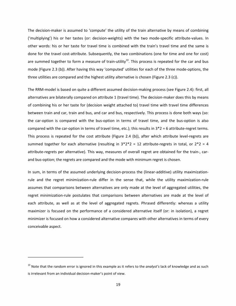
The decision-maker is assumed to ‘compute’ the utility of the train alternative by means of combining
(‘multiplying’) his or her tastes (or: decision-weights) with the two mode-specific attribute-values. In
other words: his or her taste for travel time is combined with the train’s travel time and the same is
done for the travel cost-attribute. Subsequently, the two combinations (one for time and one for cost)
are summed together to form a measure of train-utility10
. This process is repeated for the car and bus
mode (Figure 2.3 (b)). After having this way ‘computed’ utilities for each of the three mode-options, the
three utilities are compared and the highest utility alternative is chosen (Figure 2.3 (c)).
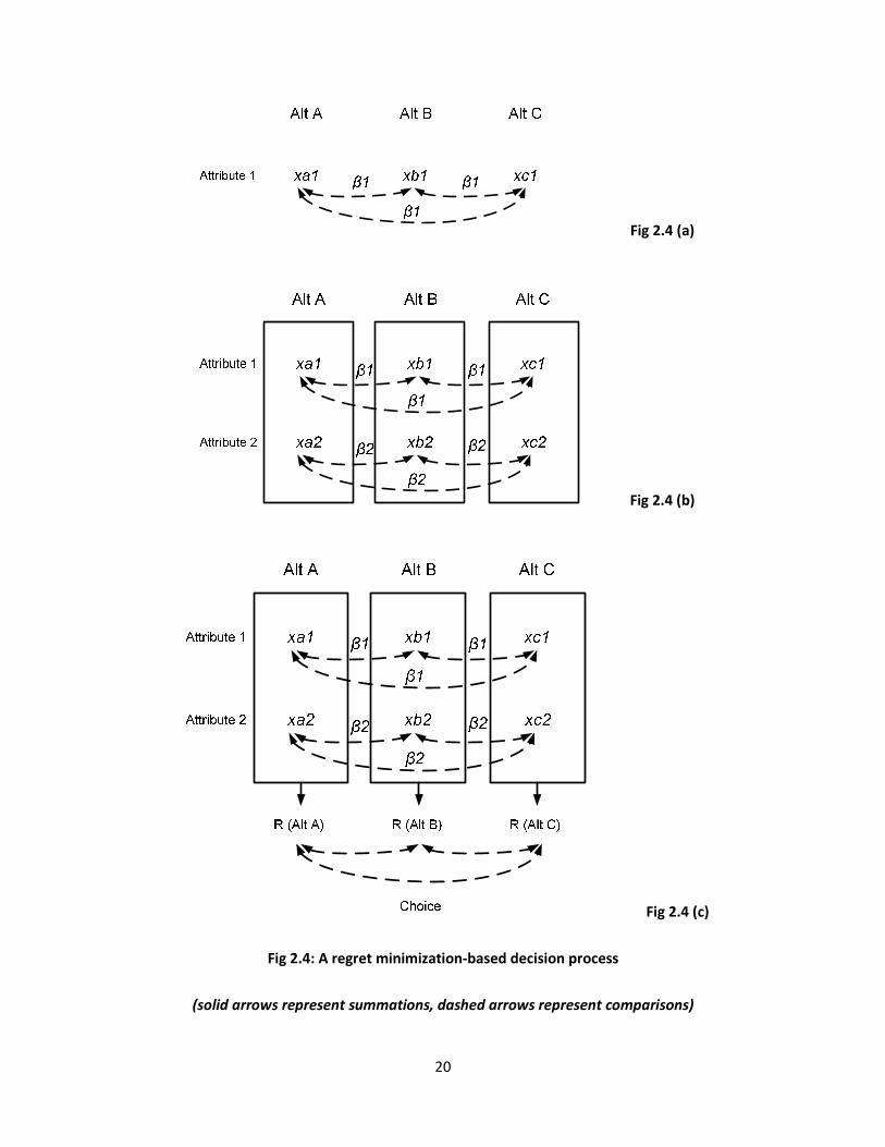
The RRM-model is based on quite a different assumed decision-making process (see Figure 2.4): first, all
alternatives are bilaterally compared on attribute 1 (travel time). The decision-maker does this by means
of combining his or her taste for (decision weight attached to) travel time with travel time differences
between train and car, train and bus, and car and bus, respectively. This process is done both ways (so:
the car-option is compared with the bus-option in terms of travel time, and the bus-option is also
compared with the car-option in terms of travel time, etc.); this results in 3*2 = 6 attribute-regret terms.
This process is repeated for the cost attribute (Figure 2.4 (b)), after which attribute level-regrets are
summed together for each alternative (resulting in 3*2*2 = 12 attribute-regrets in total, or 2*2 = 4
attribute-regrets per alternative). This way, measures of overall regret are obtained for the train-, car-
and bus-option; the regrets are compared and the mode with minimum regret is chosen.
In sum, in terms of the assumed underlying decision-process the (linear-additive) utility maximization-
rule and the regret minimization-rule differ in the sense that, while the utility maximization-rule
assumes that comparisons between alternatives are only made at the level of aggregated utilities, the
regret minimization-rule postulates that comparisons between alternatives are made at the level of
each attribute, as well as at the level of aggregated regrets. Phrased differently: whereas a utility
maximizer is focused on the performance of a considered alternative itself (or: in isolation), a regret
minimizer is focused on how a considered alternative compares with other alternatives in terms of every
conceivable aspect.
10 Note that the random error is ignored in this example as it refers to the analyst’s lack of knowledge and as such
is irrelevant from an individual decision-maker’s point of view.
20
Fig 2.4 (a)
Fig 2.4 (b)
Fig 2.4 (c)
Fig 2.4: A regret minimization-based decision process
(solid arrows represent summations, dashed arrows represent comparisons)
21
However, it should at this point again be noted that to a considerable extent the differences highlighted
above are artificial: strictly speaking, choice models do not assumed particular decision processes, and
the same mathematical model-formulation is generally consistent with a range of underlying processes.
The only formal difference between the RRM-model and a linear-additive RUM-model is that in the
former, attributes of other alternatives codetermine the utility (called regret) of a considered
alternative, and that they do so in an asymmetric, non-linear way.
As a consequence of the slightly fuzzy nature of the conceptual differences between the two models in
terms of their assumed decision processes, it is more important to discuss how the two models differ in
terms of their predictions (i.e., in terms of the choice probabilities they assign to different alternatives).
The next chapter will provide such a comparison. However, before this comparison can be made, choice
probabilities have to be derived for the RRM-model.
2.3. Regret-based choice probabilities and a RRM-based MNL-model
Having established and discussed in-depth the random regret-function (as well as how it contrasts
conceptually with its natural RUM-counterpart, the linear-additive random utility-function), the next
step is to present a regret-based choice probability-formulation which gives the probability that a
regret-minimizer chooses a particular alternative from a choice set. Obviously, should a researcher know
the total (or: random) regret associated with each alternative, then he or she can readily determine the
chosen alternative (which is the one with minimum regret). However, since part of the regret that is
associated with a particular alternative is ‘unobserved’ by the analyst as is represented by the random
error term, he or she can only predict choices up to a probability. Like is the case for RUM-models, this
formulation of this probability depends on the particular distribution assumed for the error terms. For
RUM-models it has been found (McFadden 1974) that the most convenient (because: closed form)
formulation of choice probabilities is obtained when errors are assumed to be i.i.d. Extreme Value Type
I-distributed11
. This result (leading to the RUM-based MNL-or Multinomial Logit-model of discrete
11 The term i.i.d. stands for identically and independently distributed. This means that errors assigned to different
alternatives are uncorrelated, and are drawn from the same distribution (with the same variance). This variance is
usually fixed to π2/6, which indirectly implies a normalization of systematic utility. In this tutorial, the scale of the
utility or regret is always normalized this way, and is therefore not explicitly mentioned in equations.
22
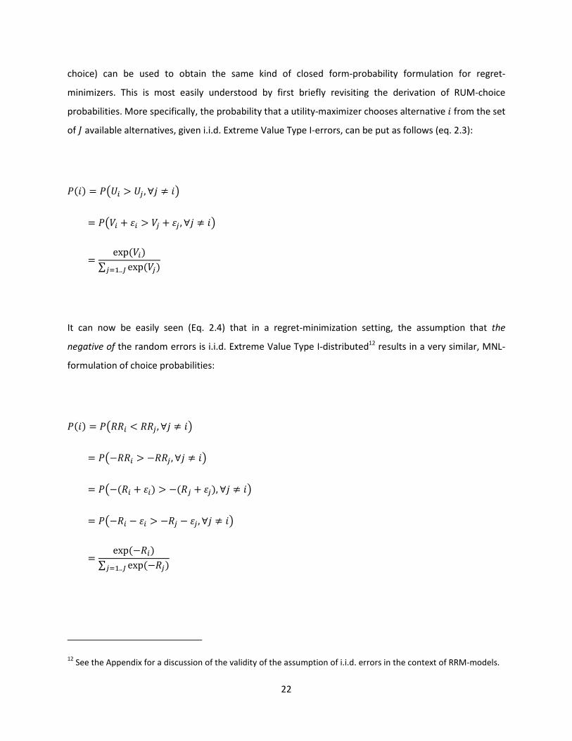
choice) can be used to obtain the same kind of closed form-probability formulation for regret-
minimizers. This is most easily understood by first briefly revisiting the derivation of RUM-choice
probabilities. More specifically, the probability that a utility-maximizer chooses alternative � from the set
of � available alternatives, given i.i.d. Extreme Value Type I-errors, can be put as follows (eq. 2.3):
./�0 � .,� 1 ,� , ∀� 3 ��
� .-� � �� 1 -� � �� , ∀� 3 ��
� exp/-�0∑ exp/-�0�56..8
It can now be easily seen (Eq. 2.4) that in a regret-minimization setting, the assumption that the
negative of the random errors is i.i.d. Extreme Value Type I-distributed12
results in a very similar, MNL-
formulation of choice probabilities:
./�0 � .��� 9 ���, ∀� 3 ��
� .���� 1 ����, ∀� 3 ��
� .�/�� � ��0 1 �/�� � ��0, ∀� 3 ��
� .��� � �� 1 ��� � ��, ∀� 3 ��
� exp/���0∑ exp/���0�56..8
12 See the Appendix for a discussion of the validity of the assumption of i.i.d. errors in the context of RRM-models.
23
The fact that the RRM-model features MNL-type choice probabilities (in combination with the fact that it
has a smooth regret-function) comes with many potential benefits. Particularly it implies that, although
the underlying behavioral premises of the RRM-model are fundamentally different from those of
conventional RUM-models (see Section 2.2), the RRM-based MNL-model can use many of the
econometric tools contained in the very comprehensive and well-understood ‘toolbox’ that has been
developed over the past three decades in the context of the RUM-based MNL-model. This includes the
use of estimation routines embedded in standard software packages.
It should be noted that, although in the remainder of this tutorial the focus will be on the MNL-model
form presented above, extension towards so-called Mixed Logit-model forms is straightforward. That is,
by adding error terms or by allowing parameters or the scale factor to vary randomly across individuals,
so-called nesting and panel effects as well as random taste- and/or scale-heterogeneity can be
accommodated in RRM-based Mixed Logit models. Translation of RRM-based MNL-models towards
RRM-based Mixed Logit models is equivalent to the translation of RUM-based MNL-models towards
RUM-based Mixed Logit models and hence will not be covered in this manual (see for example Train
(2003) for an excellent treatment of RUM-based Mixed Logit models).
Finally, it should be noted that in binary choice situations (containing only two alternatives), the RRM-
based MNL and the RUM-based MNL result in the same choice probabilities. For the interested reader, a
formal proof is provided in the appendix of Chorus (2010).

24
25
3. Empirical application of Random Regret Minimization-models
This chapter presents an in-depth discussion of how the RRM-based MNL-model is estimated, and how
estimation results are interpreted and used for forecasting. This is done by means of a comprehensive
discussion of one running example. Section 3.1 presents the dataset used for empirical analyses, while
Section 3.2 discusses RRM-model estimation. Sections 3.3 and 3.4 discuss model fit, respectively the
interpretation of estimation results, and section 3.5 shows how estimated models can be used to
forecast market shares (highlighting some of the RRM-model’s important empirical properties). Section
3.6 concludes by discussing the out-of-sample validity of the RRM-model on the given dataset.
Comparisons with the RUM-based MNL-model are provided throughout.
3.1. The data13
The data collection effort focused on route choice behavior among commuters who travel from home to
work by car. A total of 550 people were sampled from an internet panel maintained by IntoMart, in April
2011. Sampled individuals were at least 18 years old, owned a car, and were employed. It was taken
care of that the sample was representative for the Dutch commuter in terms of gender, age and
education level. Of these 550 people, 390 filled out the survey (implying a response rate of 71%).
Respondents to the survey were asked to imagine the hypothetical situation where they were planning a
new commute from home to work (either because they had recently moved, or because their employer
had recently moved, or because they had started a new job). They were asked to choose between three
different routes that differed in terms of the following four attributes, with three levels each: average
door-to-door travel time (45, 60, 75 minutes), percentage of travel time spent in traffic jams (10%, 25%,
40%), travel time variability (± 5, ± 15, ± 25 minutes), and total costs (€5.5, €9, €12.5). Using the Ngene-
software package, a so-called ‘optimal orthogonal in the differences’-design of choice sets was created
to ensure a statistically efficient data collection. This design resulted in nine choice tasks per respondent
(implying 3510 choice observations in total). An example of a route-choice task is shown in Figure 3.1.
13 See Chorus and Bierlaire (under review) for an empirical comparison of several models (including a linear-
additive RUM-model and an RRM-model) in the context of this dataset.
26
1 Route A Route B Route C
Average travel time (minutes) 45 60 75
Percentage of travel time in congestion (%) 10% 25% 40%
Travel time variability (minutes) ±5 ±15 ±25
Travel costs (Euros) €12,5 €9 €5,5
YOUR CHOICE
□
□
□
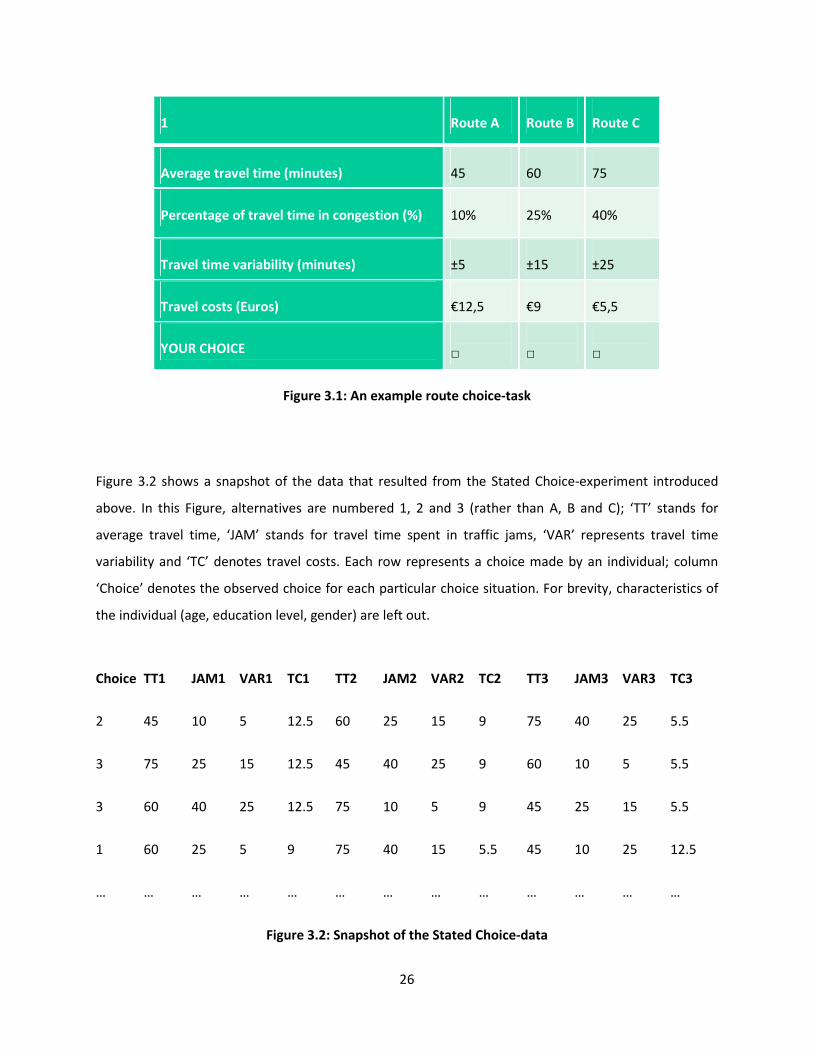
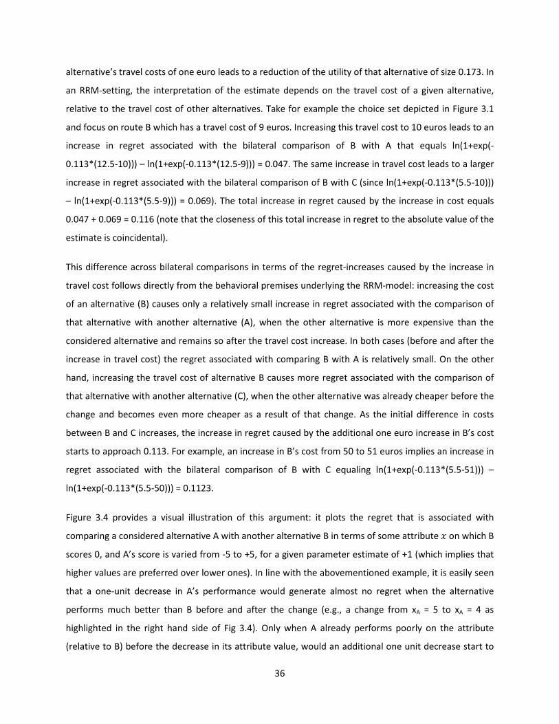
Figure 3.1: An example route choice-task
Figure 3.2 shows a snapshot of the data that resulted from the Stated Choice-experiment introduced
above. In this Figure, alternatives are numbered 1, 2 and 3 (rather than A, B and C); ‘TT’ stands for
average travel time, ‘JAM’ stands for travel time spent in traffic jams, ‘VAR’ represents travel time
variability and ‘TC’ denotes travel costs. Each row represents a choice made by an individual; column
‘Choice’ denotes the observed choice for each particular choice situation. For brevity, characteristics of
the individual (age, education level, gender) are left out.
Choice TT1 JAM1 VAR1 TC1 TT2 JAM2 VAR2 TC2 TT3 JAM3 VAR3 TC3
2 45 10 5 12.5 60 25 15 9 75 40 25 5.5
3 75 25 15 12.5 45 40 25 9 60 10 5 5.5
3 60 40 25 12.5 75 10 5 9 45 25 15 5.5
1 60 25 5 9 75 40 15 5.5 45 10 25 12.5
… … … … … … … … … … … … …
Figure 3.2: Snapshot of the Stated Choice-data
27
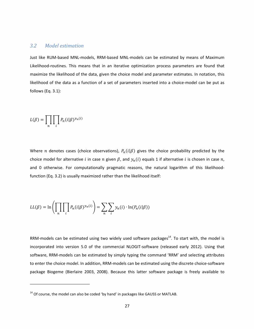
3.2 Model estimation
Just like RUM-based MNL-models, RRM-based MNL-models can be estimated by means of Maximum
Likelihood-routines. This means that in an iterative optimization process parameters are found that
maximize the likelihood of the data, given the choice model and parameter estimates. In notation, this
likelihood of the data as a function of a set of parameters inserted into a choice-model can be put as
follows (Eq. 3.1):
:/�0 �;;.</�|�0>?/�0�<
Where @ denotes cases (choice observations), .</�|�0 gives the choice probability predicted by the
choice model for alternative � in case @ given �, and A</�0 equals 1 if alternative � is chosen in case @,
and 0 otherwise. For computationally pragmatic reasons, the natural logarithm of this likelihood-
function (Eq. 3.2) is usually maximized rather than the likelihood itself:
::/�0 � ln B;;.</�|�0>?/�0�< C ���A</�0 ∙ ln/.</�|�00�<
RRM-models can be estimated using two widely used software packages14
. To start with, the model is
incorporated into version 5.0 of the commercial NLOGIT-software (released early 2012). Using that
software, RRM-models can be estimated by simply typing the command ‘RRM’ and selecting attributes
to enter the choice model. In addition, RRM-models can be estimated using the discrete choice-software
package Biogeme (Bierlaire 2003, 2008). Because this latter software package is freely available to
14 Of course, the model can also be coded ‘by hand’ in packages like GAUSS or MATLAB.
28
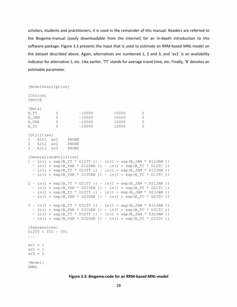
scholars, students and practitioners, it is used in the remainder of this manual. Readers are referred to
the Biogeme-manual (easily downloadable from the internet) for an in-depth introduction to this
software-package. Figure 3.3 presents the input that is used to estimate an RRM-based MNL-model on
the dataset described above. Again, alternatives are numbered 1, 2 and 3, and ‘av1’ is an availability
indicator for alternative 1, etc. Like earlier, ‘TT’ stands for average travel time, etc. Finally, ‘B’ denotes an
estimable parameter.
[ModelDescription] [Choice] CHOICE [Beta] B_TT 0 -10000 10000 0 B_JAM 0 -10000 10000 0 B_VAR 0 -10000 10000 0 B_TC 0 -10000 10000 0 [Utilities] 1 Alt1 av1 $NONE 2 Alt2 av2 $NONE 3 Alt3 av3 $NONE [GeneralizedUtilities] 1 - ln(1 + exp(B_TT * D12TT )) - ln(1 + exp(B_JAM * D12JAM )) - ln(1 + exp(B_VAR * D12VAR )) - ln(1 + exp(B_TC * D12TC )) - ln(1 + exp(B_TT * D13TT )) - ln(1 + exp(B_JAM * D13JAM )) - ln(1 + exp(B_VAR * D13VAR )) - ln(1 + exp(B_TC * D13TC )) 2 - ln(1 + exp(B_TT * D21TT )) - ln(1 + exp(B_JAM * D21JAM )) - ln(1 + exp(B_VAR * D21VAR )) - ln(1 + exp(B_TC * D21TC )) - ln(1 + exp(B_TT * D23TT )) - ln(1 + exp(B_JAM * D23JAM )) - ln(1 + exp(B_VAR * D23VAR )) - ln(1 + exp(B_TC * D23TC )) 3 - ln(1 + exp(B_TT * D31TT )) - ln(1 + exp(B_JAM * D31JAM )) - ln(1 + exp(B_VAR * D31VAR )) - ln(1 + exp(B_TC * D31TC )) - ln(1 + exp(B_TT * D32TT )) - ln(1 + exp(B_JAM * D32JAM )) - ln(1 + exp(B_VAR * D32VAR )) - ln(1 + exp(B_TC * D32TC )) [Expressions] D12TT = TT2 – TT1 ... av1 = 1 av2 = 1 av3 = 1 [Model] $MNL
Figure 3.3: Biogeme-code for an RRM-based MNL-model
29
Users acquainted with Biogeme in the context of RUM-based models will note that this code resembles
that of a RUM-based MNL-model. Note however, that the regret-function is entered under
‘GeneralizedUtilities’, rather than under ‘Utilities’. This is needed to facilitate the use of ln- and exp-
operators. Note also that minus-signs are needed to ensure that the negative of regret is maximized in
the estimation process.
Although one may insert the actual attribute-values directly in the regret-function (under
‘GeneralizedUtilities’) this results in relatively long expressions that are more cumbersome to debug
when applicable. It may be more convenient to create new variables (under ‘Expressions’) which give
the differences in attribute values that are needed in the regret-function. These new variables can then
be inserted in the regret-function, leading to a more concise and manageable formulation. Figure 3.3
shows how these new variables are constructed, for the first attribute-difference: D12TT = TT2 – TT1,
being the travel time difference relevant for the comparison of alternative 1 with 2 (note that the
difference that is relevant for the comparison of alternative 2 with 1 would read D21TT = TT1 – TT2).
It is worth noting at this point that RRM-MNL models generally take longer to estimate than RUM-MNL-
models. The reason for this difference in speed is twofold: first, RRM-MNL models generally require a
few more iteration steps before reaching convergence, although this difference tends to be small.
Secondly, and more importantly, each single iteration step consumes more computation time for a
RRM-MNL model than for its RUM-based counterpart. This is due to the simple fact that the regret-
function, with its sequence of binary comparisons and its ln- and exp-operators, involves more (and
more complicated) computations than a linear-additive utility function. Although the difference in
runtimes between RRM and RUM is inconsequential in the context of MNL-models (which generally
need seconds or at most minutes to converge), it may lead to more substantial time losses when more
complicated Mixed Logit-models are estimated, especially when datasets are very large.
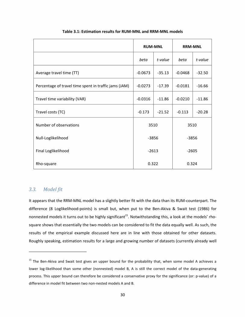
A number of observations can be made, based on the estimation results which are reported in Table 3.1.
These observations relate to either model fit or parameter estimations and significance levels.
30
Table 3.1: Estimation results for RUM-MNL and RRM-MNL models
RUM-MNL RRM-MNL
beta t-value beta t-value
Average travel time (TT) -0.0673 -35.13 -0.0468 -32.50
Percentage of travel time spent in traffic jams (JAM) -0.0273 -17.39 -0.0181 -16.66
Travel time variability (VAR) -0.0316 -11.86 -0.0210 -11.86
Travel costs (TC) -0.173 -21.52 -0.113 -20.28
Number of observations
Null-Loglikelihood
Final Loglikelihood
Rho-square
3510
-3856
-2613
0.322
3510
-3856
-2605
0.324
3.3. Model fit
It appears that the RRM-MNL model has a slightly better fit with the data than its RUM-counterpart. The
difference (8 Loglikelihood-points) is small but, when put to the Ben-Akiva & Swait test (1986) for
nonnested models it turns out to be highly significant15
. Notwithstanding this, a look at the models’ rho-
square shows that essentially the two models can be considered to fit the data equally well. As such, the
results of the empirical example discussed here are in line with those obtained for other datasets.
Roughly speaking, estimation results for a large and growing number of datasets (currently already well
15 The Ben-Akiva and Swait test gives an upper bound for the probability that, when some model A achieves a
lower log-likelihood than some other (nonnested) model B, A is still the correct model of the data-generating
process. This upper bound can therefore be considered a conservative proxy for the significance (or: p-value) of a
difference in model fit between two non-nested models A and B.
31
over 30) reveal that the RRM-MNL model outperforms its RUM-counterpart in about 50% of cases, the
RUM-MNL model doing better on the other 50%. Differences in fit are generally small, but tend to be
significant. See Chorus (2012) for a recent overview of empirical comparisons16
. Note however that, as
will be shown further below, the fact that differences in model fit are small does not imply that
parameters, predictions and policy-implications derived from estimated models are similar across the
two model types as well.
It is worth noting at this point that progress is being made to gain an understanding of what causes the
RRM-MNL model to fit some datasets better than others (when compared to RUM). Although no
definitive answers can be provided yet, empirical evidence based on sample-segmentation exercises
seems to indicate that RRM fits choice-data better than RUM to the extent that participants are
motivated and take the choice experiment seriously (in the case of Stated Choice data) and more
generally to the extent that decision-makers consider it important to make the ‘right’ decision17
.
Respondents’ motivation and their inclination to make the right decisions can be easily measured
‘directly’ using Likert-scale questions in the debriefing part of a Stated Choice experiment, for example
involving questions like “How important was it for you to make the right decision in the hypothetical
choice tasks presented to you during the experiment?”. Alternatively, respondent motivation can be
measured indirectly by means of the time taken by decision-makers to choose in the different choice
tasks (RRM-models generally fit relatively well with choice-data generated by those individuals that have
spent more time making decisions). Preliminary evidence also seems to suggest that RRM-MNL models
generally perform somewhat worse when choice-situations include a so-called ‘no-choice’ or ‘opt out’
16 Published (or in press) papers have presented empirical applications of the RRM-model and comparisons with
linear-additive RUM-models in the context of travelers’ parking choices, information acquisition, shopping
destination choices, mode-route choices (Chorus 2010), and departure time choices (Chorus & de Jong 2011);
politicians’ policy choices (Chorus et al. 2011); nature park visitors’ site choices (Thiene et al. 2012; Boeri et al. in
press); consumers’ vehicle type choices (Hensher et al. in press); and dating website-visitors’ choices among date-
profiles (Chorus & Rose in press). Studies comparing RRM and linear-additive RUM involving choices between
leisure activities by senior citizens, and choices between medical treatments by patients, are underway.
17 These empirical findings are in line with the more general notion, for which much empirical evidence exists, that
the minimization of anticipated regret is an especially important determinant of choices when decision-makers feel
that a choice is difficult and/or important (Zeelenberg & Pieters 2007).
32
option, especially when that option cannot be characterized in terms of the attributes of the actual
choice alternatives. See Chorus (2012) for a possible explanation for this preliminary finding.
3.4. Interpretation of parameters
Whereas in a RUM-setting, a parameter estimate refers to the increase or decrease in utility associated
with an alternative caused by a one-unit increase in an attribute’s value, in an RRM-setting a parameter
estimate refers to the potential (or: maximum) increase or decrease in regret associated with comparing
a considered alternative with another alternative, caused by a one unit increase in an attribute’s value.
As will be illustrated further below, whether or not this potential level of regret is indeed attained by the
increase in the attribute’s value depends on the performance of the alternative in terms of the attribute,
relative to the competition. In light of this conceptual difference between RUM- and RRM-parameters, a
number of observations can be made in terms of the interpretation of parameters presented in Table
3.1:
First, as expected, parameters have the same sign in both models and estimates are of roughly the same
order of magnitude across model types. However, these observations about magnitudes are not
particularly interesting, nor do they necessarily hold in the context of other datasets. In fact, the size of
RRM-estimates is inversely related to the size of the choice set. To see why this is the case, it should
again be noted that the regret-function used in the RRM-model (Eq. 2.1) is the sum of all the strictly
positive regrets that are generated by a series of binary comparisons with each of the other alternatives
in the set in terms of every shared attribute. Therefore, if RRM-parameters would always be of the same
size irrespective of the size of the choice set, this would imply the unrealistic scenario where in a large
choice set, regret-levels and choice probabilities are more sensitive to changes in attribute values than
they are in a smaller choice set. A much more realistic scenario would be that the degree of sensitivity of
regret-levels and choice probabilities to changes in attribute values does not depend on the choice set
size. This latter scenario implies that in the context of larger choice sets, smaller RRM-parameter
estimates should be obtained and vice versa.
This conceptual expectation can be easily confirmed empirically: first, one estimates an RRM-model on
actual or synthetic data. Then, one iteratively re-estimates the same model while, for each choice
situation, randomly selecting an increasing number of non-chosen alternatives to be unavailable for
33
choice (by doing so one gradually decreases the size of the choice set). The smaller the resulting choice
set, the larger will be the estimated RRM-parameters.
As a result of this choice set size-sensitivity of RRM-parameters, direct comparisons with their RUM-
counterparts are not particularly meaningful. Moreover, the choice set size-sensitivity of RRM-
parameters implies that when RRM-estimates are smaller (larger) than RUM-estimates on a particular
dataset, this does not mean to say that there is more (less) unobserved heterogeneity in the RRM-model
than in the RUM-model, nor that particular attributes are less (more) important in the RRM-model than
they are in the RUM-model.
Another consequence of this choice set size-dependency of RRM-estimates is that when an RRM-model
is used for market share simulation purposes (see further below for an example), the choice set used for
simulation should be of the same size as the one used for estimation in order to obtain unbiased
predictions. When the size of the choice set that is used for forecasting is (much) larger than that of the
choice set used for estimation, forecasted choice probabilities are biased towards overestimation of the
sensitivity of choice probabilities to changes in attribute values. Similarly, when the size of the choice set
that is used for forecasting is (much) smaller than that of the choice set used for estimation, forecasted
choice probabilities are biased towards underestimation of the sensitivity of choice probabilities to
changes in attribute values18
.
One would expect the abovementioned choice set size-effect not to relate to ratios of parameters as the
choice set size should affect every single parameter to the same extent. Again, this intuition can be
easily confirmed19
using synthetic data or actual choice data, by means of first estimating an RRM-model
on the actual dataset and subsequently re-estimating the same model while, for each choice situation,
randomly selecting one of the non-chosen alternatives to be unavailable for choice. Parameter ratios
obtained in the context of the two estimation processes will be of roughly the same magnitude (one
18 A particularly fruitful direction for further research would be to explore – either empirically (by means of
induction) or analytically (by means of deduction) – whether a mathematical function (or alternatively: a rule of
thumb) exists that is able to map changes in choice set-size to changes in the size of RRM-based parameter
estimates. Such a mapping or rule of thumb, if it exists, may then be used to correct parameters and eliminate
biases in forecasted probabilities, when the forecast-choice set is of a different size than the estimation-choice set.
19 This suggests that in order to attain unbiased ratios of parameter estimates in an RRM-MNL setting, one only
needs to sample the chosen alternative and a small number of non-chosen alternatives.
34
should of course allow for a small deviation which results from the randomness that is involved in the
data generation process).
As a result of this choice set-insensitivity, parameter ratios in an RRM-model can be compared in a
meaningful way with their RUM-counterparts: such a comparison gives a measurement of the
differences across model types in terms of the relative importance of one attribute relative to that of
another attribute20
. Suppose that attributes � and A have associated parameters in the context of a
RUM- and an RRM-model: �DEFG , �>EFG, �DEEG, �>EEG. Then the following result can be established in the
context of a RUM-model: for a given alternative, an increase in �’s value of ∆D units adds or removes as
much utility to or from the alternative as does an increase in A’s value of ∆D ∙ �DEFG/�>EFG units21
.
Likewise, in the context of an RRM-model, it holds that, for a given alternative, an increase in �’s value
of ∆D units has as much potential to generate or remove regret (associated with comparing the
alternative with another alternative) as does an increase in A’s value of ∆D ∙ �DEEG/�>EEG units. It is then
easily understood that parameter ratios �DEFG/�>EFG and �DEEG/�>EEG provide an indication of relative
importance of � and A in the context of the estimated RUM- and RRM-model, respectively.
To see how this type of comparison may be performed based on model estimation results, the relative
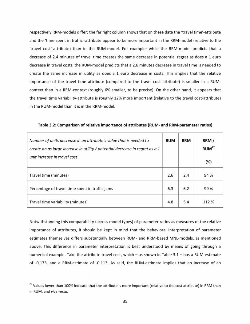
importance of RUM- and RRM-parameters presented in Table 3.1 is provided in Table 3.2. The focus is
on the situation where an alternative’s travel cost is decreased by 1 Euro. This creates an increase in
utility of 0.173 units, or a potential decrease in regret associated with comparing the alternative with
another alternative of 0.113 units. Table 3.2 presents the equivalent number of units of decrease in
other attributes that is needed to generate an as large increase in utility or potential decrease in regret.
The table clearly shows that the relative importance of attributes as implied by the estimated RUM-,
20 Of course, parameter ratios are not particularly suitable for assessing the relative importance of attributes
within the context of one and the same estimated model, since parameter ratios are sensitive to the scale of
measurement of the attributes. As such, the relative importance of for example travel time could be influenced by
simply changing the scale from minutes to hours (which would imply a sixty-fold increase of the magnitude of the
associated parameter and parameter ratios). However, as long as the same scales are used across model types,
parameter ratios can be meaningfully compared between models types, to highlight differences between model
types in terms of the relative importance of attributes.
21 In fact, when A is a cost-attribute, �DEFG/�>EFG gives the negative of the willingness-to-pay for a one unit change
in attribute �. See Chapter 5 for a discussion of an RRM-based equivalent of this willingness-to-pay concept.
35
respectively RRM-models differ: the far right column shows that on these data the ‘travel time’-attribute
and the ‘time spent in traffic’-attribute appear to be more important in the RRM-model (relative to the
‘travel cost’-attribute) than in the RUM-model. For example: while the RRM-model predicts that a
decrease of 2.4 minutes of travel time creates the same decrease in potential regret as does a 1 euro
decrease in travel costs, the RUM-model predicts that a 2.6 minutes decrease in travel time is needed to
create the same increase in utility as does a 1 euro decrease in costs. This implies that the relative
importance of the travel time attribute (compared to the travel cost attribute) is smaller in a RUM-
context than in a RRM-context (roughly 6% smaller, to be precise). On the other hand, it appears that
the travel time variability-attribute is roughly 12% more important (relative to the travel cost-attribute)
in the RUM-model than it is in the RRM-model.
Table 3.2: Comparison of relative importance of attributes (RUM- and RRM-parameter ratios)
Number of units decrease in an attribute’s value that is needed to
create an as large increase in utility / potential decrease in regret as a 1
unit increase in travel cost
RUM RRM RRM /
RUM22
(%)
Travel time (minutes) 2.6 2.4 94 %
Percentage of travel time spent in traffic jams 6.3 6.2 99 %
Travel time variability (minutes) 4.8 5.4 112 %
Notwithstanding this comparability (across model types) of parameter ratios as measures of the relative
importance of attributes, it should be kept in mind that the behavioral interpretation of parameter
estimates themselves differs substantially between RUM- and RRM-based MNL-models, as mentioned
above. This difference in parameter interpretation is best understood by means of going through a
numerical example. Take the attribute travel cost, which – as shown in Table 3.1 – has a RUM-estimate
of -0.173, and a RRM-estimate of -0.113. As said, the RUM-estimate implies that an increase of an
22 Values lower than 100% indicate that the attribute is more important (relative to the cost attribute) in RRM than
in RUM, and vice versa.
36
alternative’s travel costs of one euro leads to a reduction of the utility of that alternative of size 0.173. In
an RRM-setting, the interpretation of the estimate depends on the travel cost of a given alternative,
relative to the travel cost of other alternatives. Take for example the choice set depicted in Figure 3.1
and focus on route B which has a travel cost of 9 euros. Increasing this travel cost to 10 euros leads to an
increase in regret associated with the bilateral comparison of B with A that equals ln(1+exp(-
0.113*(12.5-10))) – ln(1+exp(-0.113*(12.5-9))) = 0.047. The same increase in travel cost leads to a larger
increase in regret associated with the bilateral comparison of B with C (since ln(1+exp(-0.113*(5.5-10)))
– ln(1+exp(-0.113*(5.5-9))) = 0.069). The total increase in regret caused by the increase in cost equals
0.047 + 0.069 = 0.116 (note that the closeness of this total increase in regret to the absolute value of the
estimate is coincidental).
This difference across bilateral comparisons in terms of the regret-increases caused by the increase in
travel cost follows directly from the behavioral premises underlying the RRM-model: increasing the cost
of an alternative (B) causes only a relatively small increase in regret associated with the comparison of
that alternative with another alternative (A), when the other alternative is more expensive than the
considered alternative and remains so after the travel cost increase. In both cases (before and after the
increase in travel cost) the regret associated with comparing B with A is relatively small. On the other
hand, increasing the travel cost of alternative B causes more regret associated with the comparison of
that alternative with another alternative (C), when the other alternative was already cheaper before the
change and becomes even more cheaper as a result of that change. As the initial difference in costs
between B and C increases, the increase in regret caused by the additional one euro increase in B’s cost
starts to approach 0.113. For example, an increase in B’s cost from 50 to 51 euros implies an increase in
regret associated with the bilateral comparison of B with C equaling ln(1+exp(-0.113*(5.5-51))) –
ln(1+exp(-0.113*(5.5-50))) = 0.1123.
Figure 3.4 provides a visual illustration of this argument: it plots the regret that is associated with
comparing a considered alternative A with another alternative B in terms of some attribute � on which B
scores 0, and A’s score is varied from -5 to +5, for a given parameter estimate of +1 (which implies that
higher values are preferred over lower ones). In line with the abovementioned example, it is easily seen
that a one-unit decrease in A’s performance would generate almost no regret when the alternative
performs much better than B before and after the change (e.g., a change from xA = 5 to xA = 4 as
highlighted in the right hand side of Fig 3.4). Only when A already performs poorly on the attribute
(relative to B) before the decrease in its attribute value, would an additional one unit decrease start to
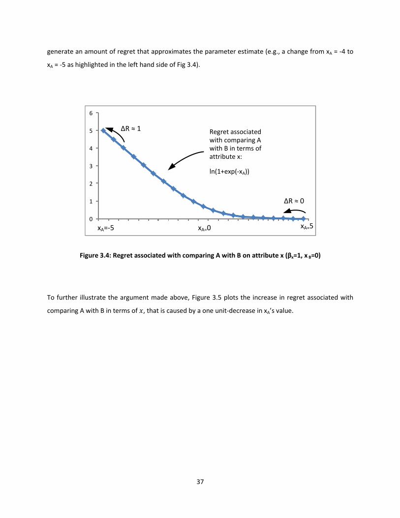
37
generate an amount of regret that approximates the parameter estimate (e.g., a change from xA = -4 to
xA = -5 as highlighted in the left hand side of Fig 3.4).
0
1
2
3
4
5
6
1 2 3 4 5 6 7 8 9 10 11 12 13 14 15 16 17 18 19 20 21xA=-5 xA=0 xA=5
Regret associated
with comparing A
with B in terms of
attribute x:
ln(1+exp(-xA))
ΔR ≈ 0
ΔR ≈ 1
Figure 3.4: Regret associated with comparing A with B on attribute x (βx=1, x B=0)
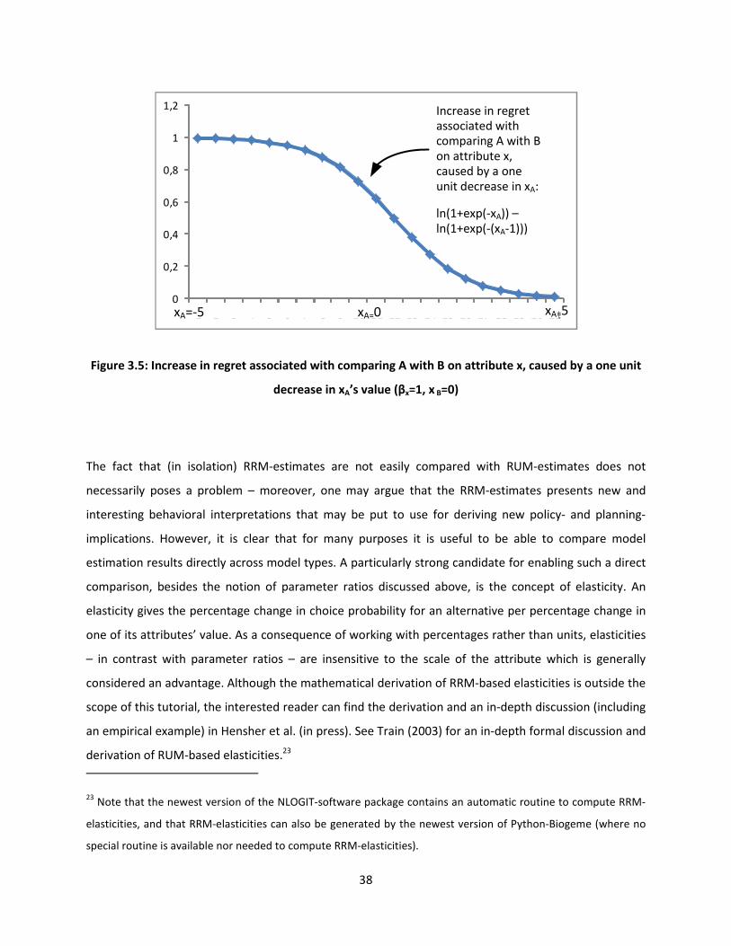
To further illustrate the argument made above, Figure 3.5 plots the increase in regret associated with
comparing A with B in terms of �, that is caused by a one unit-decrease in xA’s value.
38
0
0,2
0,4
0,6
0,8
1
1,2
1 2 3 4 5 6 7 8 9 10 11 12 13 14 15 16 17 18 19 20 21xA=-5 xA=0 xA=5
Increase in regret
associated with
comparing A with B
on attribute x,
caused by a one
unit decrease in xA:
ln(1+exp(-xA)) –
ln(1+exp(-(xA-1)))
Figure 3.5: Increase in regret associated with comparing A with B on attribute x, caused by a one unit
decrease in xA’s value (βx=1, x B=0)
The fact that (in isolation) RRM-estimates are not easily compared with RUM-estimates does not
necessarily poses a problem – moreover, one may argue that the RRM-estimates presents new and
interesting behavioral interpretations that may be put to use for deriving new policy- and planning-
implications. However, it is clear that for many purposes it is useful to be able to compare model
estimation results directly across model types. A particularly strong candidate for enabling such a direct
comparison, besides the notion of parameter ratios discussed above, is the concept of elasticity. An
elasticity gives the percentage change in choice probability for an alternative per percentage change in
one of its attributes’ value. As a consequence of working with percentages rather than units, elasticities
– in contrast with parameter ratios – are insensitive to the scale of the attribute which is generally
considered an advantage. Although the mathematical derivation of RRM-based elasticities is outside the
scope of this tutorial, the interested reader can find the derivation and an in-depth discussion (including
an empirical example) in Hensher et al. (in press). See Train (2003) for an in-depth formal discussion and
derivation of RUM-based elasticities.23
23 Note that the newest version of the NLOGIT-software package contains an automatic routine to compute RRM-
elasticities, and that RRM-elasticities can also be generated by the newest version of Python-Biogeme (where no
special routine is available nor needed to compute RRM-elasticities).
39
In both a RUM- and an RRM-setting, elasticities depend on the choice probability associated with an
alternative in a particular choice situation. As such, they are alternative- and choice situation-specific.
This is a result of the fact that the logit-model postulates (in line with intuition) that the largest impact
of a change in an attribute’s value on an alternative’s choice probability will be achieved when the
alternative is a close competitor to one or more other alternatives in the set (i.e., when the alternatives
have choice probabilities of similar magnitude). In contrast, when an alternative has a very low or a very
high choice probability, changes in its attributes’ values only have a small impact on the alternative’s
choice probability. This is why elasticities in a discrete choice-context are always computed for each
alternative and for every choice situation, after which the average is taken to obtain a sample-wide
estimate of elasticity.
In this respect, the notion of elasticity clearly contrasts with that of parameter ratios discussed further
above, since the latter are not dependent on the choice probabilities of alternatives in particular choice
situations. As such, one would not expect differences in elasticities between RRM- and RUM-based
models to fully equal differences in parameter ratios. Nevertheless, it is instructive to show the RRM-
and RUM-elasticities here (see Table 3.3) and briefly compare differences across model types with
results presented in Table 3.2. Note that since the elasticity for the ‘travel cost’ attribute is the same for
both the RRM- and RUM-model, the elasticity-ratios between model-types presented in the far-right
column of Table 3.3 for the other attributes can be compared to the ‘relative-to-cost’ ratios between
model types presented in the far-right column of Table 3.2.
40
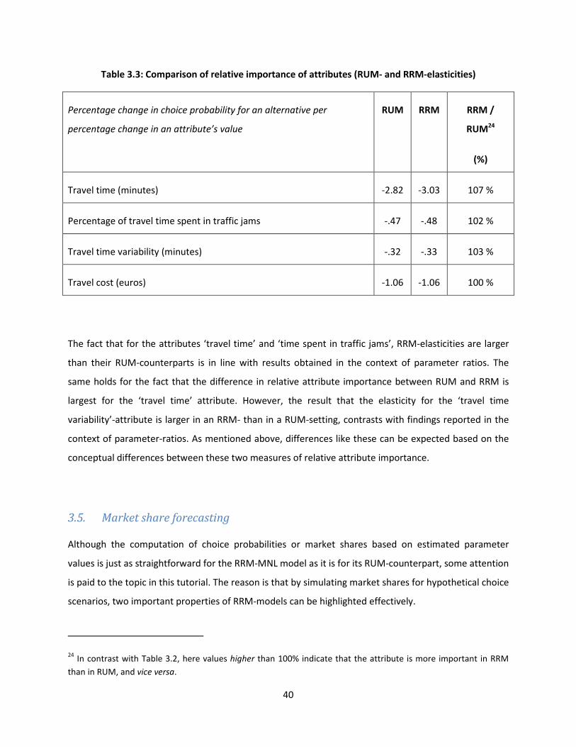
Table 3.3: Comparison of relative importance of attributes (RUM- and RRM-elasticities)
Percentage change in choice probability for an alternative per
percentage change in an attribute’s value
RUM RRM RRM /
RUM24
(%)
Travel time (minutes) -2.82 -3.03 107 %
Percentage of travel time spent in traffic jams -.47 -.48 102 %
Travel time variability (minutes) -.32 -.33 103 %
Travel cost (euros) -1.06 -1.06 100 %
The fact that for the attributes ‘travel time’ and ‘time spent in traffic jams’, RRM-elasticities are larger
than their RUM-counterparts is in line with results obtained in the context of parameter ratios. The
same holds for the fact that the difference in relative attribute importance between RUM and RRM is
largest for the ‘travel time’ attribute. However, the result that the elasticity for the ‘travel time
variability’-attribute is larger in an RRM- than in a RUM-setting, contrasts with findings reported in the
context of parameter-ratios. As mentioned above, differences like these can be expected based on the
conceptual differences between these two measures of relative attribute importance.
3.5. Market share forecasting
Although the computation of choice probabilities or market shares based on estimated parameter
values is just as straightforward for the RRM-MNL model as it is for its RUM-counterpart, some attention
is paid to the topic in this tutorial. The reason is that by simulating market shares for hypothetical choice
scenarios, two important properties of RRM-models can be highlighted effectively.
24 In contrast with Table 3.2, here values higher than 100% indicate that the attribute is more important in RRM
than in RUM, and vice versa.
41
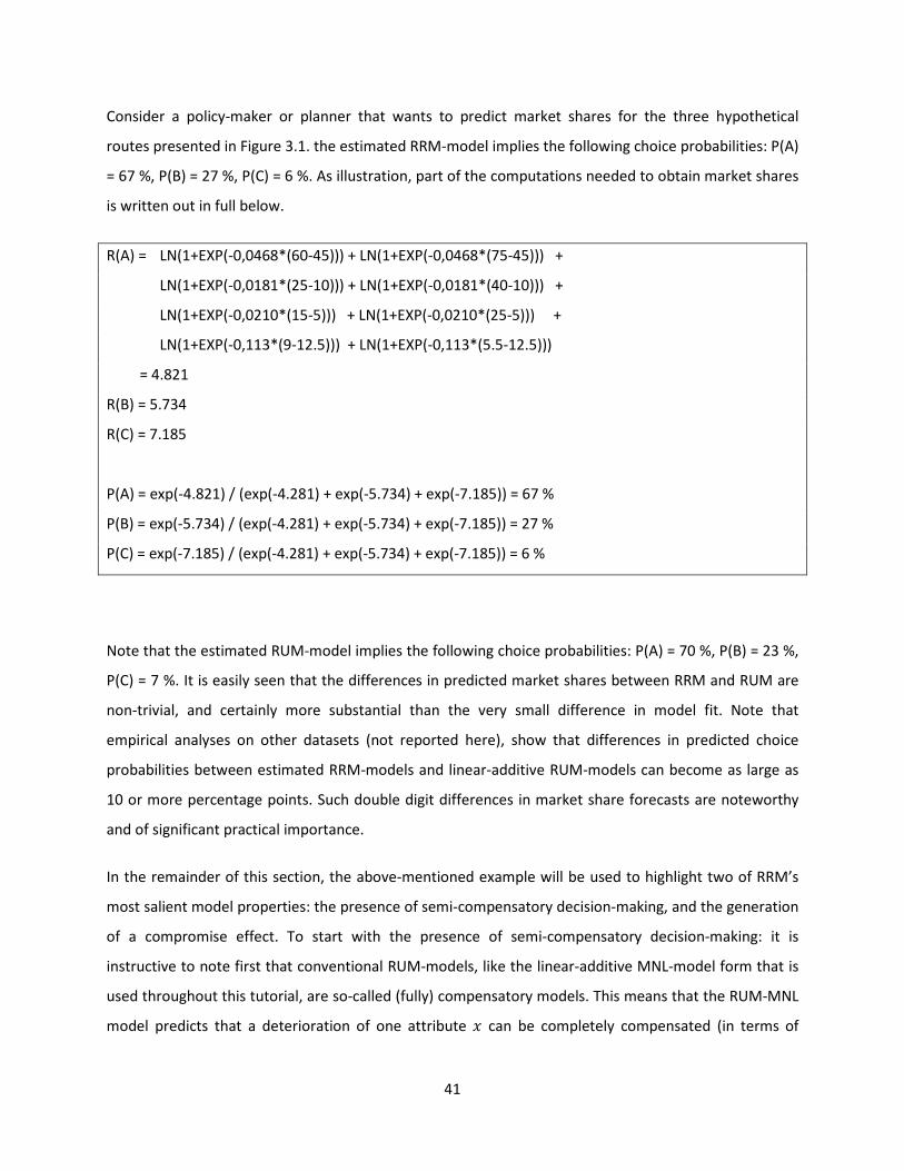
Consider a policy-maker or planner that wants to predict market shares for the three hypothetical
routes presented in Figure 3.1. the estimated RRM-model implies the following choice probabilities: P(A)
= 67 %, P(B) = 27 %, P(C) = 6 %. As illustration, part of the computations needed to obtain market shares
is written out in full below.
R(A) = LN(1+EXP(-0,0468*(60-45))) + LN(1+EXP(-0,0468*(75-45))) +
LN(1+EXP(-0,0181*(25-10))) + LN(1+EXP(-0,0181*(40-10))) +
LN(1+EXP(-0,0210*(15-5))) + LN(1+EXP(-0,0210*(25-5))) +
LN(1+EXP(-0,113*(9-12.5))) + LN(1+EXP(-0,113*(5.5-12.5)))
= 4.821
R(B) = 5.734
R(C) = 7.185
P(A) = exp(-4.821) / (exp(-4.281) + exp(-5.734) + exp(-7.185)) = 67 %
P(B) = exp(-5.734) / (exp(-4.281) + exp(-5.734) + exp(-7.185)) = 27 %
P(C) = exp(-7.185) / (exp(-4.281) + exp(-5.734) + exp(-7.185)) = 6 %
Note that the estimated RUM-model implies the following choice probabilities: P(A) = 70 %, P(B) = 23 %,
P(C) = 7 %. It is easily seen that the differences in predicted market shares between RRM and RUM are
non-trivial, and certainly more substantial than the very small difference in model fit. Note that
empirical analyses on other datasets (not reported here), show that differences in predicted choice
probabilities between estimated RRM-models and linear-additive RUM-models can become as large as
10 or more percentage points. Such double digit differences in market share forecasts are noteworthy
and of significant practical importance.
In the remainder of this section, the above-mentioned example will be used to highlight two of RRM’s
most salient model properties: the presence of semi-compensatory decision-making, and the generation
of a compromise effect. To start with the presence of semi-compensatory decision-making: it is
instructive to note first that conventional RUM-models, like the linear-additive MNL-model form that is
used throughout this tutorial, are so-called (fully) compensatory models. This means that the RUM-MNL
model predicts that a deterioration of one attribute � can be completely compensated (in terms of
42
market share) by an equally large improvement of another, equally important attribute A. Furthermore,
when the deteriorated attribute � is twice as ‘important’ as the attribute A that is improved (as would
be implied by a twice as large parameter-estimate), a twice as large improvement of A is needed to
compensate, in terms of market share, for a given deterioration of attribute �.
Take for example the two attributes travel time (RUM-parameter = -0.0673 / minute) and travel costs
(RUM-parameter = -0.173 / euro). By simulating market shares, it can be seen that 0.39 euros are
needed to compensate, in terms of market share, for a one minute increase in travel time. Note that it is
no coincidence that this value equals the ratio of parameters for time and cost (0.39 = 0.0673 / 0.173).
Importantly, in a linear-additive RUM-model, needed levels of compensation do not depend on the
initial relative performance of the alternatives in terms of the relevant attributes (travel time and cost).
In other words, the obtained value of 0.39 euros which is needed to compensate for a one minute
increase in travel time holds for each of the alternatives A, B and C in the choice situation depicted in
Figure 3.1, irrespective of their differences in performance in terms of travel time and costs.
In an RRM-MNL model things are quite different. To see this, let’s compute in the context of the
estimated RRM-MNL model the reduction in travel costs that is needed to offset a loss in market share
caused by a one minute increase in travel time. It will become clear that the needed level of
compensation depends on how the alternative performs (in terms of time and costs) relative to the
other alternatives in the set. Take for example alternative A, which is a fast but expensive route. A one
minute increase in travel time would require a 0.3 euro reduction in travel costs to compensate for this
loss in market share. Now take alternative C, which is a slow but cheap route. A one minute increase in
travel time would require a 0.5 euro reduction in travel costs to compensate for this loss in market
share. It is directly seen that this difference between the two alternatives, in terms of the level of
compensation needed to offset a one minute increase in travel time, is substantial. Yet, the difference is
easily explained by building on the reasoning presented earlier in this chapter.
More specifically, it should be noted first that the one minute increase in travel time of route A causes
only a small increase in regret, since that route is by far the fastest one, and remains so after the
marginal increase in travel time. In contrast, the alternative is a poor performer in terms of travel costs
(relative to the other two alternatives), and as such a decrease in cost causes a relatively large decrease
in regret. This implies that a (relatively) small cost decrease can compensate for the one minute increase
in travel time. For alternative C, the situation is exactly opposite: it is already the slowest route in the
43
choice set, and as such a further increase in travel time causes a relatively large increase in regret. On
the other hand, because it is the cheapest route, further reductions in travel costs result in only small
reductions in regret. In combination, this implies that a relatively large reduction in travel cost is needed
to compensate for the one minute increase in travel time.
The above-mentioned difference is arguably the most important difference between RRM and linear-
additive RUM in terms of predicted choice probabilities: in contrast with the linear-additive RUM-model,
the RRM-model predicts that the level of improvement of one attribute that is needed to compensate
(in terms of market share) a deterioration of another attribute depends on how the alternative
performs, relative to the other alternatives, in terms of both attributes. This also implies that when
some attribute (�) that is deteriorated is equally important as another one (A) that is improved (i.e.,
parameter estimates are the same), and the magnitude of the deterioration equals the magnitude of the
improvement, the improvement in A does not necessarily compensate for deterioration in �. As such,
RRM is a so-called semi-compensatory model. As illustrated by the above example, the particular type of
semi-compensatory nature exhibited by RRM-models makes that they can lead to markedly different
policy implications when compared to linear-additive RUM-models, also when model fits and even
parameter ratios are very similar across models.
The existence of so-called compromise effects, which is the second distinguishing RRM-model property
that will be discussed in this chapter, follows directly from this particular brand of semi-compensatory
behavior exhibited by RRM. The compromise effect, which is widely documented in empirical studies in
consumer choice (e.g., Kivetz et al. 2004), states that there is a market share-bonus associated with
being positioned ‘in between’ other available alternatives in terms of attribute-performance. In the
choice situation depicted in Figure 3.1, alternative B is such an ‘in between’ or ‘compromise’ alternative:
while alternatives A and C have ‘extreme’ values for each of the attributes relative to the competition,
alternative B always scores right in between: it is not the fastest route (which is A), but also not the
slowest one (C); it is not the cheapest route (C), but also not the most expensive one (A), etc. when
comparing market shares between model types, it becomes clear that the RRM-MNL model predicts a
higher market share (27 %) for this compromise alternative than does the RUM-MNL model (23 %). This
difference in predicted shares (4 percentage points or roughly 17%) suggests that the RRM-model
predicts a compromise effect (i.e., a market share bonus for the compromise alternative).
44
To see that this is indeed the case, the following line of argumentation may be used: as argued
extensively in section 3.3, the RRM-model predicts that having a (very) poor performance on one
attribute causes much regret, while having a (very) strong performance on another attribute does not
necessarily compensate for this (very) poor performance. As a result, it is more efficient (in terms of
avoiding regret and as such gaining market share) to ‘move to the center’ of the choice set: an
alternative that fails to have a really strong performance on any of the attributes (relative to the other
alternatives) still only generates modest levels of regret as long as it does not have a particularly poor
performance on any of the attributes either. This implies that alternative B, being a compromise
alternative with a moderate performance on each attribute, has a relatively high market share in the
context of an RRM-model (27 %) when compared to a linear-additive RUM-model (23 %).25
Note that the fact that RRM-models feature the compromise effect also implies that they do not exhibit
the so-called IIA-property that characterizes linear-additive RUM-MNL models, even when errors are
assumed to be i.i.d. (as is the case in the RRM-MNL model form). The IIA property says that the ratio of
choice probabilities of any two alternatives is not affected by having a new alternative enter the choice
set, nor by changing the performance of another alternative in the choice set. In contrast, RRM-models
(including the MNL-model form) postulate that any ratio of choice-probabilities can be, and even is likely
to be, affected by the presence of new alternatives or by changes in performance of any third
alternative. For example, RRM-models postulate that when the attribute-levels of alternative B are
changed to make alternative C a compromise alternative (i.e., positioned in between A and B), this leads
to an increase of the choice probability ratio P(C) / P(A).
It is important to note here that by not exhibiting the IIA-property, RRM-MNL models do not yet deal
with the type of IIA-property commonly referred to as the ‘red bus-blue bus problem’. This latter type of
IIA – from which RRM’s MNL also suffers, just like RUM’s linear-additive MNL-model – originates from
ignored correlations between the error terms of competing alternatives, and can be addressed in an
RRM-framework in a similar way as in a RUM-framework: by creating nests in Nested or Mixed Logit
model-extensions.
25 See Chorus & Bierlaire (under review) for an in-depth analysis of models that are able to capture compromise
effects (including the RRM-model), based on these data.
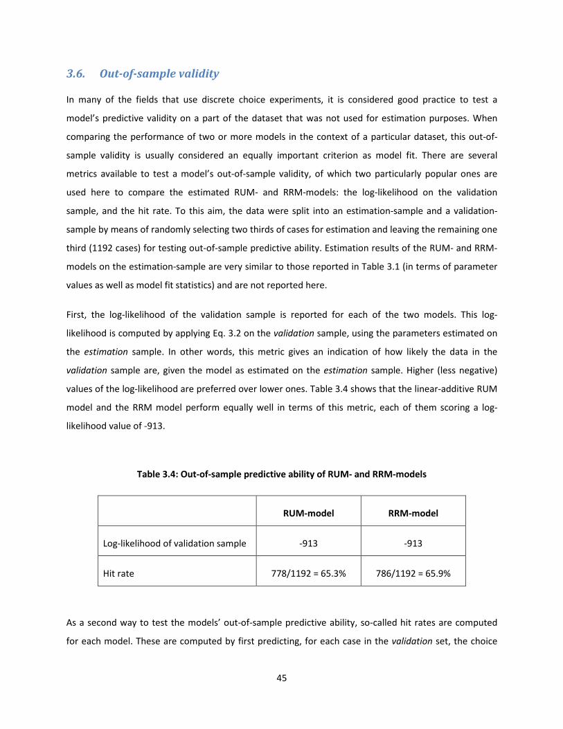
45
3.6. Out-of-sample validity
In many of the fields that use discrete choice experiments, it is considered good practice to test a
model’s predictive validity on a part of the dataset that was not used for estimation purposes. When
comparing the performance of two or more models in the context of a particular dataset, this out-of-
sample validity is usually considered an equally important criterion as model fit. There are several
metrics available to test a model’s out-of-sample validity, of which two particularly popular ones are
used here to compare the estimated RUM- and RRM-models: the log-likelihood on the validation
sample, and the hit rate. To this aim, the data were split into an estimation-sample and a validation-
sample by means of randomly selecting two thirds of cases for estimation and leaving the remaining one
third (1192 cases) for testing out-of-sample predictive ability. Estimation results of the RUM- and RRM-
models on the estimation-sample are very similar to those reported in Table 3.1 (in terms of parameter
values as well as model fit statistics) and are not reported here.
First, the log-likelihood of the validation sample is reported for each of the two models. This log-
likelihood is computed by applying Eq. 3.2 on the validation sample, using the parameters estimated on
the estimation sample. In other words, this metric gives an indication of how likely the data in the
validation sample are, given the model as estimated on the estimation sample. Higher (less negative)
values of the log-likelihood are preferred over lower ones. Table 3.4 shows that the linear-additive RUM
model and the RRM model perform equally well in terms of this metric, each of them scoring a log-
likelihood value of -913.
Table 3.4: Out-of-sample predictive ability of RUM- and RRM-models
RUM-model RRM-model
Log-likelihood of validation sample -913 -913
Hit rate 778/1192 = 65.3% 786/1192 = 65.9%
As a second way to test the models’ out-of-sample predictive ability, so-called hit rates are computed
for each model. These are computed by first predicting, for each case in the validation set, the choice
46
probabilities for every alternative using the RUM- and RRM-models as estimated on the estimation set
(see the previous section for an explanation of how these choice probabilities or ‘market shares’ are
computed). Subsequently, for each case in the validation sample and for both the RUM and the RRM
model, the alternative that has the highest predicted choice probability is compared with the actually
chosen alternative. If the two alternatives (predicted and observed) coincide, a score of one is obtained
for that case, and otherwise a score of zero. Higher hit rates are of course preferred over lower ones.
Results are as follows: the linear-additive RUM model has a hit rate of 778/1192 = 65.3%, while the
RRM-model achieves a hit rate of 786/1192 = 65.9%. Although differences are fairly small, it does appear
that the RRM-model slightly outperforms the linear-additive MNL-model when it comes to identifying
the most popular alternative in the choice sets.
To conclude, it should be noted here that – as was the case with model fit comparisons – the relative
out-of-sample performance of RUM- and RRM-models differs across datasets. As of now, there is no
conclusive evidence of one model performing consistently better than another model in terms of, for
example, out-of-sample log-likelihood or hit rate (nor is such evidence to be expected). It is found,
moreover, that differences in model fit between RUM- and RRM-models are not necessarily good
predictors for the direction of differences in out-of-sample predictive ability; i.e., many situations occur
where one model does better in terms of model fit, while the other model does better in terms of one
or more out-of-sample predictive ability metrics. This is in a way to be expected, given the probabilistic
nature of discrete choice models.
47
4. Applicability of Random Regret Minimization-models , and their
strong and weak points
This chapter starts (section 4.1) with discussing the applicability of the RRM-model in other than the
quite straightforward choice context presented in Chapter 3. More specifically, it is explained how RRM
can be applied to model non-generic attributes, constants, non-continuous attributes, and interactions
with socio-demographic variables. Subsequently, section 4.2 and 4.3 present strong, respectively weak
points of the RRM-model.
4.1. General applicability
The empirical example presented in Chapter 3 was based on a choice situation that is particularly
intuitive to explain the working of RRM-models, in the sense that it featured a choice situation where
alternatives were presented in terms of generic attributes (i.e., attributes that are shared by all
alternatives) that were also continuous. The notion of regret is particularly easy to understand and
model in such a context, as illustrated in that Chapter. However, the RRM-approach can also be readily
applied in choice situations where one or more attributes are non-generic and/or non-continuous; in
these situations, a number of approaches can be chosen.
4.1.1. Non-generic attributes
Sometimes, the analyst might want to specify one or more attributes in a way that they are specific to
only one or a subset of the alternatives in the choice set: take for example the situation where a choice
set contains car and train alternatives and a researcher wants to estimate travel time-parameters for
each of these two modes separately (i.e., he or she wants to estimate �JJKLM, �JJNML�<), to account for the
fact that train-travel time may be valued differently than car-travel time. In such a situation, the RRM-
model can be applied by simply constructing the following function for, for example, the regret
associated with comparing a car option with a train option in terms of their travel times: �JJKLM �ln1 � exp��JJNML�< ∙ OONML�< � �JJKLM ∙ OOKLM��. When considering that ln1 � exp��� ∙ ��� � ������ =
ln1 � exp��� ∙ ��� � �� ∙ ������, it is easily seen that the implementation of non-generic attributes
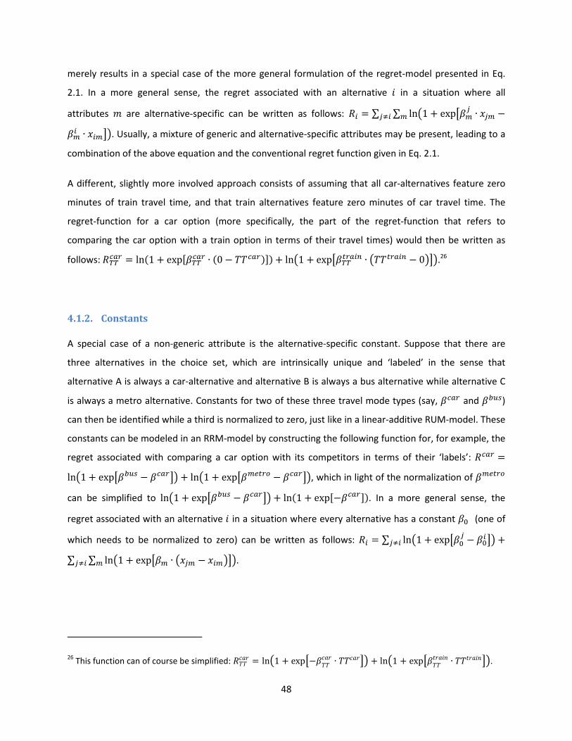
48
merely results in a special case of the more general formulation of the regret-model presented in Eq.
2.1. In a more general sense, the regret associated with an alternative � in a situation where all
attributes P are alternative-specific can be written as follows: �� � ∑ ∑ ln1 � exp���� ∙ ��� �������� ∙ �����. Usually, a mixture of generic and alternative-specific attributes may be present, leading to a
combination of the above equation and the conventional regret function given in Eq. 2.1.
A different, slightly more involved approach consists of assuming that all car-alternatives feature zero
minutes of train travel time, and that train alternatives feature zero minutes of car travel time. The
regret-function for a car option (more specifically, the part of the regret-function that refers to
comparing the car option with a train option in terms of their travel times) would then be written as
follows:�JJKLM � ln/1 � expQ�JJKLM ∙ /0 � OOKLM0R0 � ln1 � exp��JJNML�< ∙ OONML�< � 0���.26
4.1.2. Constants
A special case of a non-generic attribute is the alternative-specific constant. Suppose that there are
three alternatives in the choice set, which are intrinsically unique and ‘labeled’ in the sense that
alternative A is always a car-alternative and alternative B is always a bus alternative while alternative C
is always a metro alternative. Constants for two of these three travel mode types (say, �KLM and �STU)
can then be identified while a third is normalized to zero, just like in a linear-additive RUM-model. These
constants can be modeled in an RRM-model by constructing the following function for, for example, the
regret associated with comparing a car option with its competitors in terms of their ‘labels’: �KLM �ln1 � exp��STU � �KLM�� � ln1 � exp���VNMW � �KLM��, which in light of the normalization of ��VNMW
can be simplified to ln1 � exp��STU � �KLM�� � ln/1 � expQ��KLMR0. In a more general sense, the
regret associated with an alternative � in a situation where every alternative has a constant �X (one of
which needs to be normalized to zero) can be written as follows: �� � ∑ ln1 � exp��X� � �X� ����� �∑ ∑ ln1 � exp��� ∙ ��� � ���������� .
26 This function can of course be simplified: �OOYZ[ � ln1 � exp���OOYZ[ ∙ OOYZ[�� � ln1 � exp��OO\[Z�@ ∙ OO\[Z�@��.
49
4.1.3. Non-continuous (categorical) attributes
Next is the issue of the implementation of non-continuous attributes: take for example the situation
where a choice set contains a number of train options, which differ in terms of – among other attributes
– the availability of wireless internet. More specifically, suppose that the internet-availability attribute
can take on the value ‘no internet’, ‘internet for a 1 euro fee’ and ‘internet for free’. In this case, the
attribute is clearly non-continuous and there is no single parameter that is likely to describe the
preference of travelers for the entire attribute-range. This kind of variables can be dealt with in an RRM-
model as follows: first, like is the case in a linear-additive RUM-model, two dummy variables (0/1-
variables) are created to represent the three-category non-continuous attribute internet availability’,
and whose associated parameters will be estimated. More specifically: each category is represented by a
dummy, minus one category (parameter) which needs to be normalized (to zero) to ensure
identification.
Suppose that ‘no internet’ is considered the base level, implying that an ‘internet for a 1 euro fee’-
dummy (�]VV) and an ‘internet for free’-dummy (�]MVV) are created for each alternative. This in turn
implies that parameters �]VV and �]MVV are estimated. Assume a particular trinary choice-situation
where alternative A is of type ‘no access’, and that B is of type ‘access for a 1 euro fee’, while C is of type
‘free access’.27
Now, just like would the case in a linear-additive RUM-setting, the following dummies are
created: �]VV^ � �]MVV^ � 0; �]VV` � 1, �]MVV` � 0; �]VVa � 0, �]MVVa � 1. The part the regret-function of
alternative A (‘no access’) that relates to comparing the alternative with, for example, alternative B
(‘access for a 1 euro fee’) in terms of internet-availability then can be written as follows: ��<N^ �ln1 � exp��]VV` ∙ �]VV` � �]MVV` ∙ �]MVV` � �]VV^ ∙ �]VV^ � �]MVV^ ∙ �]MVV^ ���, which for this particular case
can be simplified to ��<N^ � ln1 � exp��]VV` ��. In the above formulation the term ‘�]VV` ∙ �]VV` � �]MVV` ∙�]MVV` ’ refers to the performance of B in terms of internet-availability (higher values lead to more regret
for A) and the term ‘�]VV^ ∙ �]VV^ � �]MVV^ ∙ �]MVV^ ’ refers to the performance of A in terms of internet-
availability (higher values lead to less regret for A). Regrets associated with comparing A with C, B with
A, B with C, C with A and C with B are derived in a similar fashion.
27 It is important to note here that if type A would always be of type ‘no access’, etc., this would imply that
experiment is de facto labeled and that the approache outlined in 4.1.2 should be used instead: preferences for
types are then treated as constants. The text in 4.1.3 refers to the situation where A’s type (as well as that of B and
C) varies across cases in the dataset.
50
4.1.4. Hybrid RUM-RRM models
Notwithstanding that the approaches outlined above provide effective means to deal with non-generic
variables (including constants) and/or non-continuous variables in regret-functions, it is instructive to
note that these kinds of variables can also be treated ‘outside’ the regret-function, as utilitarian
variables. More generally speaking, one may choose to position one or more attributes outside the
regret-function while having others enter the regret-function. Behaviorally, such a hybrid model implies
that some attributes are assumed by the researcher to be processed by the decision-maker in a linear-
additive RUM-way, while others are assumed to be processed in a RRM-fashion. If there are b attributes
being implemented outside the regret function, and � � b inside the regret function, the systematic
part of such a hybrid utility/regret-function would look like this (Eq. 4.1):
-� � � �� ∙�56..c ��� �� � ln1 � exp��� ∙ ��� � �������5cd6..G���
Choice probabilities are given by the utility-based MNL formulation given in Eq. 2.3. Preliminary
empirical analyses (Chorus et al. under review) show that for approximately one out of every three
datasets, a hybrid model-specification achieves a higher model fit and/or out-of-sample validity than a
model that assumes only RUM-heuristics or only RRM-heuristics for each and every attribute.
4.1.5. Interactions with socio-demographic variables
Besides being able to deal with non-generic and non-continuous variables as shown above, the RRM-
model also readily applies to situations where individual-level or socio-demographic variables are
interacted with constants and/or attribute-level parameters. More specifically, this is done in almost the
exact same way as in linear-additive RUM: take for example a parameter referring to a price-attribute
(�eM�KV), which is interacted with the individual-level variable ‘Zfg’ to represent the fact that different
age-segments may have different tastes for that attribute. This is simply done by replacing in the all
regret functions �eM�KV by �eM�KV � �eM�KVLhV ∙ Zfg. Parameter �eM�KVLhV then refers to the additional regret
that is caused by a particular price-difference between two alternatives, for a one-year age increase. A
51
similar formulation holds for interactions with constants. Hensher et al. (in press) provide an empirical
example of an RRM-model including socio-demographic interactions.
4.2. RRM: strong points
It is increasingly acknowledged that the RRM-model in a number of ways provides an appealing
alternative to conventional RUM-models. First, its regret-based premises provide a behaviorally intuitive
alternative to the utility-maximization paradigm that has dominated the field of choice modeling and
related fields for decades. Many feel that it pays off (in terms of insights gained) to study discrete
choice-behavior from different behavioral perspectives, and the RRM-model provides an intuitive and
formally tractable way of doing so. The RRM-model ‘tells a story’ that is fundamentally different from
the linear-additive RUM-storyline, and as such it may lead to new behavioral insights and new policy-
and planning-implications.
Furthermore, there is ample evidence from all corners of the social sciences (see Zeelenberg & Pieters
(2007) for an overview) that the anticipation of regret is an important determinant of choice behavior;
the RRM paradigm provides an opportunity to translate this notion into an operational discrete choice-
modeling perspective. In addition, two of RRM’s most important properties (semi-compensatory
decision-making and the existence of a compromise-effect) have been well-established empirically in
numerous studies. In a RRM-model context, these properties readily emerge from the model’s
underlying behavioral premises.
In addition, the RRM-model appears to do well empirically: on many datasets (around 50% of those
studies so far) RRM-models achieve a better model fit and/or out-of-sample validity than their RUM-
counterparts. At the aggregate level of the dataset, differences between RRM and linear-additive RUM
in terms of model fit and out-of-sample validity are generally small. However, estimation results and
derived quantities – such as parameter ratios, elasticities and simulated choice probabilities for
particular policy scenarios – may differ quite substantially across models. As such, the RRM-approach
presents a new behavioral model perspective that has a considerable policy-relevance.
When compared to other so-called non-RUM models, RRM-models have the advantage of being very
parsimonious (they consume no additional parameters compared to RUM’s most basic linear-additive
model form), while at the same time remaining quite user-friendly and compatible with (or:
52
incorporated in) some of the field’s most-used software packages. As such, perhaps more than many
other non-RUM models, the RRM-model is a viable option also for those modelers that lack the time or
econometric experience to code and apply highly complex choice models.
4.3. RRM: weak points
Having mentioned these strong points, it is clear that the RRM-model has its drawbacks and limitations
as well. The issue of run-times was mentioned earlier in this tutorial: especially in the context of Mixed
Logit models and very large datasets, RRM-models take considerably more time to converge than their
RUM-counterparts. The author’s experience suggests that RRM run-times may become twice or three
times as high as RUM run-times, depending on the error term specification in Mixed Logit models, the
number of attributes, and the choice set size. For some applications, this might limit the applicability of
RRM-models. Note however, that in the context of most MNL-models, run-times are not an issue at all.
A related issue is that of combinatorial explosion: since RRM’s regret functions involve comparisons with
each alternative in the choice set on every attribute, there is a risk of combinatorial explosion: run-times
grow faster than linearly as a function of choice set size. Although most choice sets encountered in
discrete choice studies deal with choice sets of small or moderate size, some studies (e.g. some
destination choice studies) involve very large choice sets of hundreds or even thousands of alternatives,
which would lead to prohibitively high run-times for RRM-models28
.
More generally speaking, the RRM-MNL model – while being more ‘simple’ than most other non-RUM
models – is still slightly more complex than RUM’s workhorse, the linear additive MNL-model. As is
shown in chapter 3, the difference in complexity between the two paradigms is hardly noticeable when
dealing with small choice sets, small numbers of attributes and simple specifications involving no
interactions with socio-demographic variables. However, for the analysis of more involved choice
28 However, it may be noted that the behavioral realism of the assumption that decision-makers would actually
consider dozens, let alone hundreds, of alternatives when choosing is increasingly debated in fields like travel
behavior as well as consumer psychology. As a result, more and more researchers call for the use of small choice
sets in choice model estimation and application, even when in practice the universal set of alternatives may be
very large.
53
situations, the RRM-model can become somewhat more cumbersome to code and interpret than the
RUM-MNL model.
Finally, the fact that the RRM-model is relatively new – which is an appealing characteristic for some
modelers, especially in academia – may prove a disadvantage as well, for example when it comes to
communicating results to policy-makers and planners. Furthermore, it is obvious that the RRM-model is
not yet as well understood as its counterpart, the linear-additive RUM-MNL model. For example, it is not
yet completely clear how the RRM-model can be used for economic appraisal, although progress is
being made in this regard (e.g., Chorus & de Jong 2011; Chorus 2012; Chorus under review (b) – see also
sections 5.3 and 5.4 in the next Chapter). This clearly contrasts with linear-additive RUM-models’ level of
applicability for economic appraisal, which has been well-documented over the past few decades. The
topic of economic appraisal is just one example of the still considerable knowledge-gap that exists
between RRM and linear-additive RUM-models.
However, considering the amount of attention currently being devoted to the RRM-model by a growing
number of choice-modelers it may be expected that in time this knowledge gap will diminish, making
the RRM-model an increasingly competitive alternative to linear-additive RUM-models. Take for
example Bekhor et al. (in press), who derive and apply an RRM-based Stochastic User Equilibrium (as a
counterpart of the conventional RUM-based Stochastic User Equilibrium) which enables the regret-
based prediction of equilibrium traffic flows on transport networks. The next chapter discusses a
number of research areas where recent attempts have been made to further increase the scope and
usefulness of RRM.

54
55
5. Selection of recent developments in RRM-modeling
Very recently, a number of developments have taken place that have further broadened the scope of
the Random Regret Minimization approach to discrete choice modeling. This chapter provides brief
introductions to some of these developments, without aiming to be complete with respect to the
number of developments covered nor the amount of detail provided for any one particular
development. Instead, this chapter’s sections aim to provide some first insights into these recent
developments. Wherever relevant, references are provided to research papers providing more
elaborate discussions. Avenues for further research are discussed at the end of each section. Finally note
that these recent developments are discussed here in the context of transportation-related choices.
However, relevance and implications for other fields can be easily seen. Sections 5.1, 5.3, and 5.4 draw
from recently published papers or papers that are currently in press. Citations are provided wherever
relevant.
5.1. Random regret minimization for decision-making under uncertainty29
The term ‘uncertainty’ here refers to situations where decision-makers, at the time they make a
decision, are not certain about the values of (some of) the attributes of alternatives under
consideration. Take for example a traveler that chooses between different routes, but cannot assess
with full certainty what travel times he or she may encounter during the trip. Therefore, the choice
between routes is generally a choice under uncertainty, and the traveler is then assumed to take into
account this uncertainty when making decisions.
Extending the RRM-approach towards the context of analyzing decisions made under uncertainty is
relatively straightforward, and similar to the extension of (Random) Utility Theory to (Random) Expected
Utility Theory. Assume that a traveler conceives uncertainty in terms of the possibility of occurrence of
different states of the world i, where each state has a (perceived) probability of occurrence. These
29 This section draws from Chorus (2012).
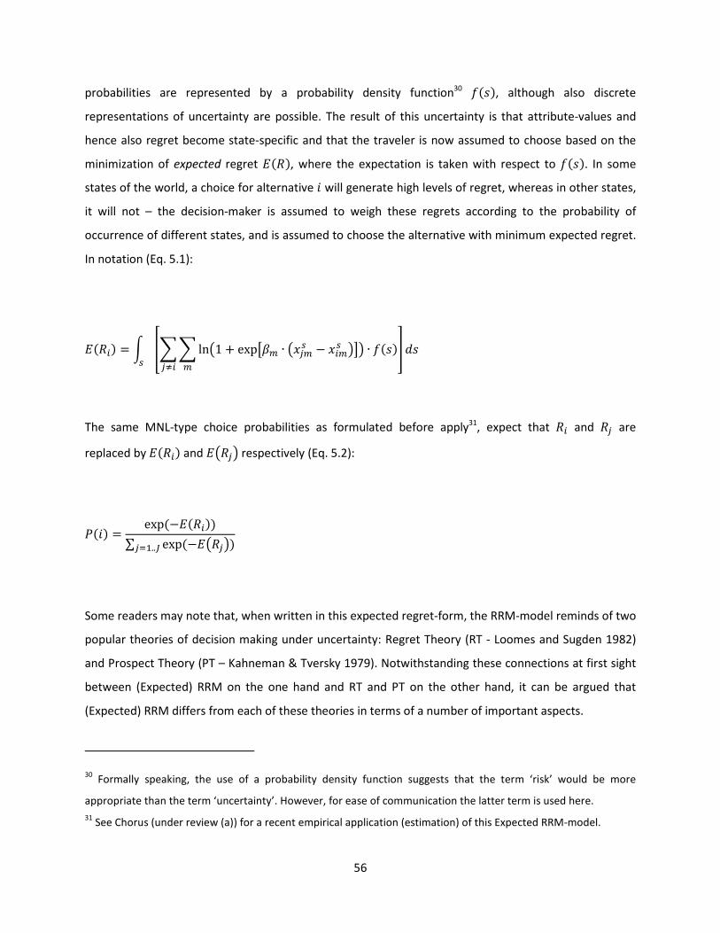
56
probabilities are represented by a probability density function30
j/i0, although also discrete
representations of uncertainty are possible. The result of this uncertainty is that attribute-values and
hence also regret become state-specific and that the traveler is now assumed to choose based on the
minimization of expected regret k/�0, where the expectation is taken with respect to j/i0. In some
states of the world, a choice for alternative � will generate high levels of regret, whereas in other states,
it will not – the decision-maker is assumed to weigh these regrets according to the probability of
occurrence of different states, and is assumed to choose the alternative with minimum expected regret.
In notation (Eq. 5.1):
k/��0 � l m��ln1 � exp��� ∙ ���U � ���U ������� ∙ j/i0n oiU
The same MNL-type choice probabilities as formulated before apply31
, expect that �� and �� are
replaced by k/��0 and k���respectively (Eq. 5.2):
./�0 � exp/�k/��00∑ exp/�k���0�56..8
Some readers may note that, when written in this expected regret-form, the RRM-model reminds of two
popular theories of decision making under uncertainty: Regret Theory (RT - Loomes and Sugden 1982)
and Prospect Theory (PT – Kahneman & Tversky 1979). Notwithstanding these connections at first sight
between (Expected) RRM on the one hand and RT and PT on the other hand, it can be argued that
(Expected) RRM differs from each of these theories in terms of a number of important aspects.
30 Formally speaking, the use of a probability density function suggests that the term ‘risk’ would be more
appropriate than the term ‘uncertainty’. However, for ease of communication the latter term is used here.
31 See Chorus (under review (a)) for a recent empirical application (estimation) of this Expected RRM-model.
57
First, RT focuses on decision-making under uncertainty only and is designed with the aim to capture
choice-anomalies that are not being dealt with in neoclassical Expected Utility-theory, like preference
reversals and common ratio effects. In contrast, while RRM may be extended towards the analysis of
decision-making under uncertainty as shown above, it is primarily developed for the analysis of choice
under conditions of full certainty, where it captures semi-compensatory choice behavior and choice set-
composition effects. Second, while RT is focused on the study of single-attribute choices often used in
the field of behavioral and experimental economics (mostly involving monetary gambles), RRM is
explicitly designed to model choices between multi-attribute alternatives like those presented in Stated
Choice-experiments often used in the field of, for example, travel demand and consumer choice
analysis. Thirdly, where RT postulates that regret arises by comparing the utilities of alternatives, RRM
postulates that regret by comparing alternatives in terms of each of their attributes: the essence of RRM
lies in its hypothesis that when making multi-attribute choices, regret arises from the likely situation
where one has to put up with a relatively poor performance on one or more attributes to arrive at a
relatively strong performance on other attributes. These three conceptual differences between RRM
and RT in combination translate into substantial differences in formal regret-functions, predictions and
scope / applicability. As a result, it makes more sense conceptually to position RRM-theory as a regret-
based counterpart of linear-additive RUM-theory, rather than a discrete choice-counterpart of Regret
Theory.
The connection between RRM and Prospect Theory (PT) follows from the fact that both postulate that
the evaluation of an alternative depends on its performance relative to a reference point, and that
losses compared to that reference point loom larger than gains of the same magnitude. But also here,
the differences between the two choice-theories are larger than the seemingly unifying concept of
reference-dependency would suggest. Firstly, RRM’s reference points are given by the attribute-level
performance of foregone alternatives, whereas PT’s reference point is generally given by some
operationalization of the status quo (or: current wealth). As a result, whereas PT postulates that
preferences are context-dependent, RRM claims that they are choice set-dependent. Secondly, RRM
captures loss aversion in a different way than does PT, beyond the difference in adopted reference
point. More specifically, RRM assumes that the consideration of gains does not matter at all while PT
assumes that perceived gains are still a substantial determinant of choice behavior. Furthermore, the
RRM-model features no additional parameter(s), like PT does, to measure the degree of loss aversion.
Thirdly, whereas PT is explicitly positioned as a model of decision-making under uncertainty (featuring a
58
probability-weighting function to represent potential probability-distortions), RRM is tailored for choice-
situations where attribute-values are known to the decision-maker and as such it features no behavioral
postulates concerning how people deal with probabilities beyond the use of a probability density
function as outlined above. In sum: although at first sight RRM’s use of a reference point may suggest a
deep connection between RRM and PT, this connection is not that intuitive and persuasive when more
profoundly inspecting the two theories of choice.
An important avenue for further research is to empirically test how RRM (using the notion of expected
regret) compares to linear-additive RUM (using the notion of expected utility) in the context of decision-
making under uncertainty. In addition, empirical comparisons with non-Expected Utility models such as
Prospect Theory-based models are needed to determine how each of these decision-making models
performs empirically.
5.2 RRM for modeling household or group decision-making
Many choices are made a group or household level, rather than by one individual in isolation. Take for
example the situation where a household decides where to go on vacation. In a RUM-setting, this
household decision making process has been traditionally modeled by assuming a household utility
function which represents the aggregated utilities of all members. It is assumed that the household
trades off the utilities assigned by different household members to various choice options, using weights
that represent the ‘importance’ or ‘bargaining power’ of different members. Recent work suggests that
the RRM-framework can provide a particularly intuitive alternative modeling framework for these
household (or: group) decision-making processes. The focus is here on the modeling framework at a
conceptual level, rather than on data-issues and model estimation processes.
In notation: denote choice-alternatives by �, �. Denote individuals by p (and assume there are q
individuals in the household). Denote the regret that an individual member of the household p attaches
to an alternative � by ��r. Denote the importance, or bargaining power, of individual p within the
household by sr. It may then be postulated that, when choosing between alternatives, households aim
to minimize (anticipated) random household regret, and that the level of random household regret that
is associated with a considered alternative � is composed of an i.i.d. random error, which represents
unobserved heterogeneity in household regret and whose negative is Extreme Value Type I-distributed,
59
and a systematic household regret t��. The core of this systematic household regret is the following
term (Eq. 5.3):
t��↔�r � ln1 � exp�sr ∙ ��r � ��r���
t��↔�r gives the amount of household regret that is associated with comparing the regrets that are
associated with alternative � and � respectively, as anticipated by member p. Here, ��r � ∑ ∑ ln1 �����exp���r ∙ ���r � ���r ��� gives the amount of regret that is associated with alternative �, as anticipated
by member p. If � has a lower regret than � in the eye of this particular household member, then the
comparison of ��r with ��r generates (almost) zero household regret. When � has a higher regret than � in the eye of the household member, then the comparison of ��r with ��r generates a level of household
regret that grows as a semi-linear function of the importance of the household member and the
difference between ��r and ��r (in the eye of that member). Note that the indexation of ���r , ���r and ��r
with respect to p implies that perceptions and preferences of members with respect to the attributes of
alternatives are member specific. Note furthermore, that the above formulation does not specify
random errors at the level of the regret anticipated by individual household members. However, these
can be added and accommodated by using an error component Mixed Logit formulation at the
household member level32
.
The term t��↔�r discussed above is computed for each household member, and for all binary
comparisons between the considered alternative � and every other alternative � 3 �. Systematic over-all
household regret is then the sum of all these terms (Eq. 5.4):
32
At this point it may also be noted that rather than assuming regret-minimization calculus at both the level of the
household and the level of the household member, one may assume that while a household minimizes regret,
every member of the household maximizes a linear-additive utility function. In that case the term ��r � ��r in Eq.
5.3 becomes -�r � -�r, and these utilities can be written as in Eq. 2.2, with indexation for the household member.
60
t�� �� � t��↔�rr56..v��� �� � ln1 � exp�sr ∙ ��r � ��r���r56..v���
The same MNL-type choice-probabilities as given in Eq. 2.4 apply. The difference between this
household regret function and the individual-level regret function discussed earlier in this tutorial can be
put as follows: the individual-level regret function that is discussed throughout this tutorial refers to
weighing the performance of different alternatives in terms of their attributes. Weights represent the
importance of attributes. In contrast, the household level formulation of the regret function discussed in
this section refers to weighing the performance of different alternatives in terms of the regret (or:
utility) they generate for particular household members. Weights represent the importance or
bargaining power of those members. The household regret function incorporates the individual level
regret function to represent the preferences of its members, although this individual level regret
function may also be replaced by an individual level utility function.
Conceptually, the difference between an RRM and a linear-additive RUM approach to modeling group
decision making is that the former assumes that a group aims to minimize regret at a group level, and as
such is likely to choose compromise alternatives which are not extremely disliked by any of the
household members. In contrast, using a compensatory decision rule at the group level like that of
linear-additive RUM-models would presuppose that the dislike of one household member can be readily
compensated for by the satisfaction of another member. Intuitively, one would expect that many group
decision making processes result in compromises to make sure that no particular group member is
deeply unsatisfied with the outcome of the decision-making process. As such the RRM-approach is likely
to be a particularly effective and intuitive modeling paradigm for such group decision-making processes.
However, a very obvious direction for further research is to empirically compare the performance of the
RRM-based group decision making model with that of the mainstream linear-additive RUM-based
approach. Work is underway to perform such a test, using data on household decision-making in the
context of vehicle purchases.
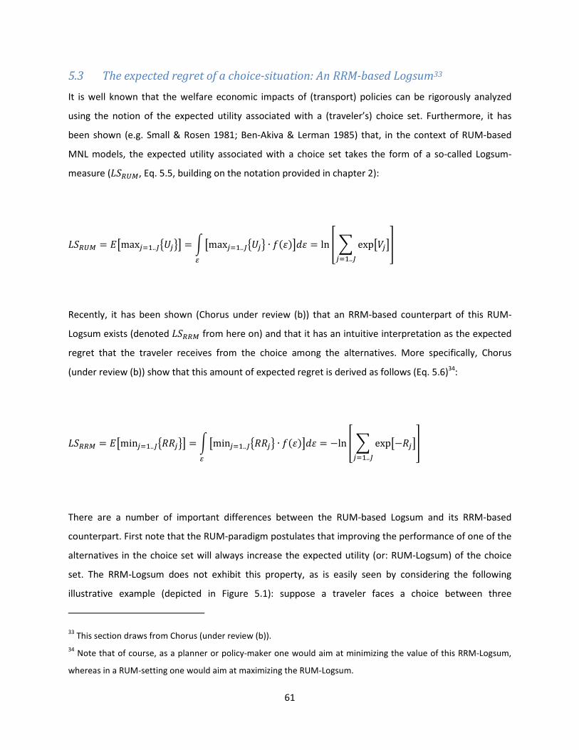
61
5.3 The expected regret of a choice-situation: An RRM-based Logsum33
It is well known that the welfare economic impacts of (transport) policies can be rigorously analyzed
using the notion of the expected utility associated with a (traveler’s) choice set. Furthermore, it has
been shown (e.g. Small & Rosen 1981; Ben-Akiva & Lerman 1985) that, in the context of RUM-based
MNL models, the expected utility associated with a choice set takes the form of a so-called Logsum-
measure (:wEFG, Eq. 5.5, building on the notation provided in chapter 2):
:wEFG � k�max�56..8x,�y� � l�max�56..8x,�y ∙ j/�0�o�z � ln m � exp�-���56..8 n
Recently, it has been shown (Chorus under review (b)) that an RRM-based counterpart of this RUM-
Logsum exists (denoted :wEEG from here on) and that it has an intuitive interpretation as the expected
regret that the traveler receives from the choice among the alternatives. More specifically, Chorus
(under review (b)) show that this amount of expected regret is derived as follows (Eq. 5.6)34
:
:wEEG � k�min�56..8x���y� � l�min�56..8x���y ∙ j/�0�o�z � �ln m � exp������56..8 n
There are a number of important differences between the RUM-based Logsum and its RRM-based
counterpart. First note that the RUM-paradigm postulates that improving the performance of one of the
alternatives in the choice set will always increase the expected utility (or: RUM-Logsum) of the choice
set. The RRM-Logsum does not exhibit this property, as is easily seen by considering the following
illustrative example (depicted in Figure 5.1): suppose a traveler faces a choice between three
33 This section draws from Chorus (under review (b)).
34 Note that of course, as a planner or policy-maker one would aim at minimizing the value of this RRM-Logsum,
whereas in a RUM-setting one would aim at maximizing the RUM-Logsum.
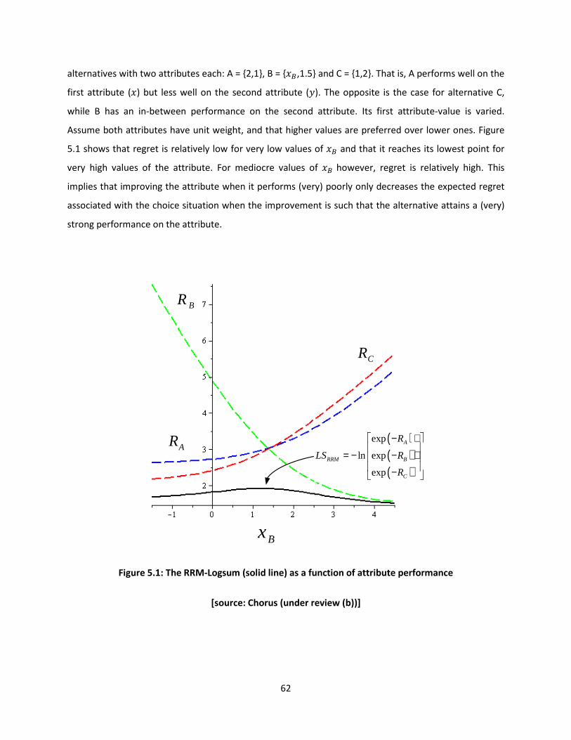
62
alternatives with two attributes each: A = {2,1}, B = {�`,1.5} and C = {1,2}. That is, A performs well on the
first attribute (�) but less well on the second attribute (A). The opposite is the case for alternative C,
while B has an in-between performance on the second attribute. Its first attribute-value is varied.
Assume both attributes have unit weight, and that higher values are preferred over lower ones. Figure
5.1 shows that regret is relatively low for very low values of �` and that it reaches its lowest point for
very high values of the attribute. For mediocre values of �` however, regret is relatively high. This
implies that improving the attribute when it performs (very) poorly only decreases the expected regret
associated with the choice situation when the improvement is such that the alternative attains a (very)
strong performance on the attribute.
( )( )( )
exp
ln exp
exp
A
RRM B
C
R
LS R
R
− +
= − − + −
AR
BR
CR
Bx
Figure 5.1: The RRM-Logsum (solid line) as a function of attribute performance
[source: Chorus (under review (b))]
63
The behavioral intuition behind this non-monotonicity of the RRM-Logsum can be put as follows: when
alternative B has a very poor performance on attribute �, this makes that there is a very high level of
regret associated with that alternative. However, this very high level of regret for the alternative does
not translate into a high level of expected regret for the choice situation, because there are alternatives
with much lower regrets available. Furthermore, the fact that B performs poorly on � implies that
alternatives A and C have relatively low regrets (since comparisons with B barely generate regret at all).
When �` attains a more intermediate value, B’s regret decreases but the regrets associated with the
other two alternatives increase since now, the comparison of A and C with B does generate some regret.
The result is a situation where all regrets are of roughly similar magnitude, and that the expected regret
associated with the choice situation increases – because the regret associated with the alternative(s)
with lowest regrets (A, C) increases. Only when �` becomes very large, does the expected regret
associated with the choice situation start to decline: in that situation, the regret associated with A and C
grows, but since B’s regret is now (much) lower than these two regrets this increase in A’s and B’s regret
becomes more and more irrelevant. The fact that B’s regret declines therefore finally starts resulting in a
lower level of expected regret associated with the choice situation as a whole. Only when �` becomes
very high, a lower level of expected regret is obtained than was associated with the situation when B
performed very poorly on �.
In general, in can be said that a change in the choice set that makes the traveler’s decision more difficult
– in the sense that due to the change there is no clear ‘winner’ among the alternatives – will increase
the expected regret associated with the choice situation. Changes that do create clear winners, even
when this comes at the cost of a deteriorating the performance of one or more alternatives, will lead to
a decrease in expected regret associated with the choice situation. Note that this property of the RRM-
Logsum is in fact in line with consumer research that suggests that larger choice sets without clear
‘winners’ may be considered less attractive by decision-makers than small sets containing a clear
‘winner’ (e.g., Schwartz et al. 2002).
A particularly interesting direction for further research would be to investigate how the RRM-Logsum
relates to welfare economic principles. As mentioned above, it has been well-established that the RUM-
Logsum has a strong and very elegant foundation in neoclassical welfare theory. This rigorous
connection has led to a substantial popularity of the RUM-Logsum in transport project (infrastructure
investment) evaluations. It is at this point not yet clear to what extent the RRM-Logsum can be
considered a valid and useful welfare measure (beyond its natural interpretation of the expected regret
64
associated with a choice situation), and establishing to what extent it is (in-)consistent with welfare
economics may be considered a potentially very fruitful research direction.
5.4 An RRM-based formulation of ‘Value of Time’35
It is very well known that in a linear-additive RUM-MNL model context involving travel choices, the ratio
of partial derivatives of the utility function with respect to the travel time attribute (denoted TT) and the
travel cost attribute (TC) has an intuitive interpretation as the Value of Time (VoT from here on). This
VoT gives the amount of money that a traveler is willing to pay for a one unit decrease in travel time36
.
As such, the notion of VoT is crucial input in quantitative evaluations of transport policies such as
policies aimed at decreasing congestion (travel times) in traffic networks. In the context of linear-
additive RUM-MNL models, this ratio of partial derivatives results in a very easy-to-compute and
interpret formulation (Eq. 5.7):
-|OEFG � }-�}OO� }-�}O~�� � �JJ�Ja
In other words, VoT in a linear-additive RUM-MNL context is given by the ratio of the parameters
estimated for the travel time and travel cost-attributes. The RRM-counterpart of this ratio of partial
derivatives takes on a quite different form (Eq. 5.8):
35 This sections draws from Chorus (2012).
36 More in general, the ratio of partial derivatives of a utility function with respect to one of its attributes and the
cost attribute gives the (negative of the) willingness to pay for a one unit increase in the non-cost attribute.
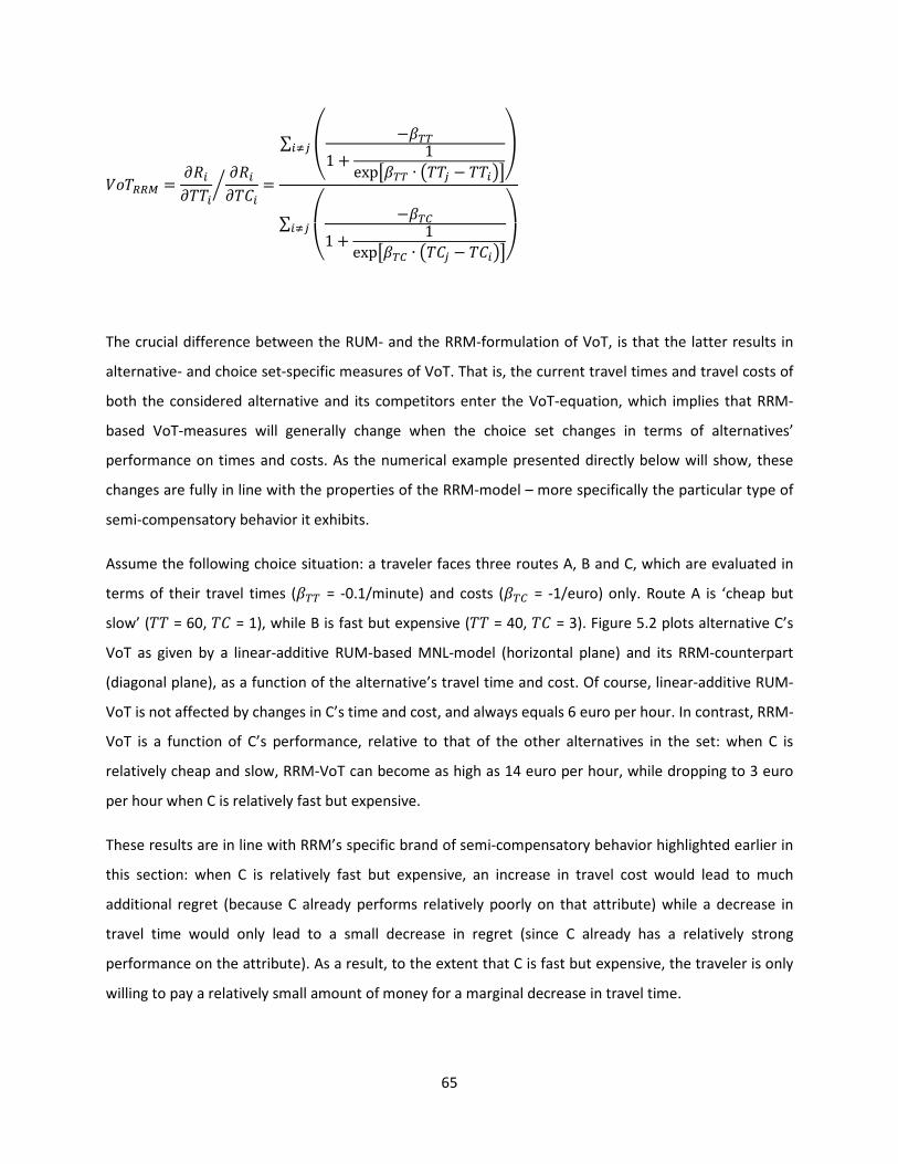
65
-|OEEG � }��}OO� }��}O~�� �∑
�� ��JJ1 � 1exp��JJ ∙ OO� � OO����
����
∑�� ��Ja1 � 1exp��Ja ∙ O~� � O~����
����
The crucial difference between the RUM- and the RRM-formulation of VoT, is that the latter results in
alternative- and choice set-specific measures of VoT. That is, the current travel times and travel costs of
both the considered alternative and its competitors enter the VoT-equation, which implies that RRM-
based VoT-measures will generally change when the choice set changes in terms of alternatives’
performance on times and costs. As the numerical example presented directly below will show, these
changes are fully in line with the properties of the RRM-model – more specifically the particular type of
semi-compensatory behavior it exhibits.
Assume the following choice situation: a traveler faces three routes A, B and C, which are evaluated in
terms of their travel times (�JJ = -0.1/minute) and costs (�Ja = -1/euro) only. Route A is ‘cheap but
slow’ (OO = 60, O~ = 1), while B is fast but expensive (OO = 40, O~ = 3). Figure 5.2 plots alternative C’s
VoT as given by a linear-additive RUM-based MNL-model (horizontal plane) and its RRM-counterpart
(diagonal plane), as a function of the alternative’s travel time and cost. Of course, linear-additive RUM-
VoT is not affected by changes in C’s time and cost, and always equals 6 euro per hour. In contrast, RRM-
VoT is a function of C’s performance, relative to that of the other alternatives in the set: when C is
relatively cheap and slow, RRM-VoT can become as high as 14 euro per hour, while dropping to 3 euro
per hour when C is relatively fast but expensive.
These results are in line with RRM’s specific brand of semi-compensatory behavior highlighted earlier in
this section: when C is relatively fast but expensive, an increase in travel cost would lead to much
additional regret (because C already performs relatively poorly on that attribute) while a decrease in
travel time would only lead to a small decrease in regret (since C already has a relatively strong
performance on the attribute). As a result, to the extent that C is fast but expensive, the traveler is only
willing to pay a relatively small amount of money for a marginal decrease in travel time.
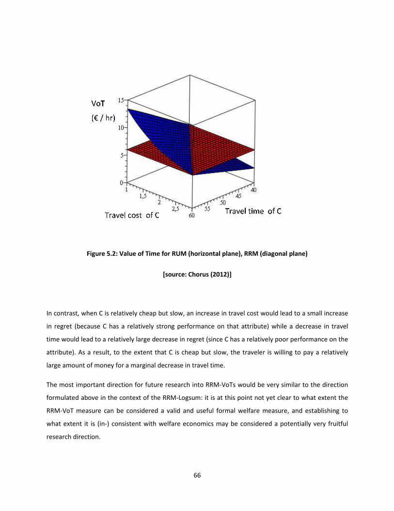
66
Figure 5.2: Value of Time for RUM (horizontal plane), RRM (diagonal plane)
[source: Chorus (2012)]
In contrast, when C is relatively cheap but slow, an increase in travel cost would lead to a small increase
in regret (because C has a relatively strong performance on that attribute) while a decrease in travel
time would lead to a relatively large decrease in regret (since C has a relatively poor performance on the
attribute). As a result, to the extent that C is cheap but slow, the traveler is willing to pay a relatively
large amount of money for a marginal decrease in travel time.
The most important direction for future research into RRM-VoTs would be very similar to the direction
formulated above in the context of the RRM-Logsum: it is at this point not yet clear to what extent the
RRM-VoT measure can be considered a valid and useful formal welfare measure, and establishing to
what extent it is (in-) consistent with welfare economics may be considered a potentially very fruitful
research direction.
67
References
Bekhor S, Chorus CG, Toledo T (in press) A Stochastic User Equilibrium formulation for the Random
Regret Minimization-based route choice model. Transport Res Rec
Ben-Akiva ME, Lerman SR (1985) Discrete choice analysis: theory and application to travel demand. The
MIT Press, Cambridge, Mass
Ben-Akiva ME, Swait J (1986) The Akaike likelihood ratio index. Transport Sci 20:133-136
Bierlaire M (2003) Biogeme: A free package for the estimation of discrete choice models, Proceedings of
the 3rd Swiss Transportation Research Conference, Ascona, Switzerland.
Bierlaire M (2008) An introduction to BIOGEME Version 1.7, biogeme.epfl.ch
Boeri M, Longo A, Doherty E, Hynes S (in press) Site choices in recreational demand: A matter of utility
maximization or regret minimization? J Env Econ Pol. doi:10.1080/21606544.2011.640844
Chorus CG, Arentze TA, Timmermans HJP (2008) A Random Regret Minimization model of travel choice.
Transport Res B 42:1-18
Chorus CG, Arentze TA, Timmermans HJP (2009) Spatial choice: A matter of utility or regret? Environ
Plann B 36:538-551
Chorus CG (2010) A new model of Random Regret Minimization. Eur J of Transp Infrast 10:181-196
Chorus CG, de Jong GC (2011) Modeling experienced accessibility for utility-maximizers and regret-
minimizers. J Transp Geog 19:1155-1162
Chorus, CG, Annema, JA, Mouter, N, van Wee, GP (2011) Modeling politicians' preferences for road
pricing policies: A regret-based and utilitarian perspective. Transp Policy 18:856-861
Chorus CG (2012) Random Regret Minimization: An overview of model properties and empirical
evidence. Transport Rev 32:75-92
Chorus CG, Rose JK (in press) Selecting a date: A matter of regret and compromises. In: Hess S & Daly A
(Eds.) Choice modelling: the state of the art and the state of practice: Selected papers from the Second
International Choice Modelling Conference, Edward Elgar, UK
Chorus CG (under review (a)) Valuating ex-post travel information: A matter of balancing regrets
Chorus CG (under review (b)) Logsums for utility-maximizers and regret-minimizers, and their relation
with desirability and satisfaction
68
Chorus CG, Rose JM, Hensher DA (under review) Regret minimization or utility maximization: It depends
on the attribute.
Chorus CG, Bierlaire M (under review) An empirical comparison of travel choice models that generate
compromise effects
Hensher DA, Rose JM, Greene WH (2005) Applied choice analysis: A primer. Cambridge University Press,
Cambridge, United Kingdom
Hensher DA, Greene W, Chorus CG (in press) Random Regret Minimisation or Random Utility
Maximisation: An exploratory analysis in the context of automobile fuel choice. J Adv Transport. doi:
10.1002/atr.188
Hess S, Stathopoulos A, Daly A (in press) Mixing of behavioral processes: A modeling framework and
three case-studies. Transportation. doi:10.1007/s11116-011-9365-6
Kivetz R, Netzer O, Srinivasan V (2004) Alternative models for capturing the compromise effect. J
Marketing Res 41:237-257
Kahneman D, Tversky A (1979) Prospect Theory: An analysis of decision under risk. Econometrica
47:263-291
Loomes G, Sugden R (1982) Regret Theory: An alternative theory of rational choice under uncertainty.
Econ J 92:805-824
McFadden D (1974) Conditional logit analysis of qualitative choice-behavior. In Zarembka P, (Ed.)
Frontiers in econometrics, Academic Press, New York
Schwartz B, Ward A, Monterosso J, Lyubomirsky S, White K, Lehman DR (2002) Maximizing versus
satisficing: Happiness is a matter of choice. J Pers Soc Psychol 83:1178-1197
Small KA, Rosen HS (1981) Applied welfare economics with discrete choice models. Econometrica
49:105-130
Thiene M, Boeri M, Chorus CG (2012) Random Regret Minimization: Exploration of a new choice model
for environmental and resource economics. Environ Resour Econ 51:413-429
Train KE (2003) Discrete choice methods with simulations. Cambridge University Press, Cambridge UK
Zeelenberg M, Pieters R (2007) A theory of regret regulation 1.0. J Consum Psychol 17:3-18
69
Appendix: Investigating the assumption of i.i.d. errors in RRM-models
Like RUM-based MNL-models, RRM’s MNL-model assumes that random errors are independent
(uncorrelated) across alternatives. This assumption, which is a crucial condition for obtaining closed
form choice probabilities, may appear counterintuitive at first sight because of the fact that an
alternative’s observed regret is a function of the performance of the alternative relative to that of all
other alternatives in the choice set. One may ask: how can the random component of a considered
alternative’s regret be safely assumed to be independent from other alternatives’ random regrets, when
the observed regret of the considered alternative is a function of the performance of all alternatives in
terms of observed attributes? More specifically, one may be inclined to expect that if one alternative’s
unobserved regret decreases, the unobserved regret of a randomly selected competing alternative must
increase. In this Appendix, an argumentation is provided for the use of independent (or: uncorrelated)
errors in RRM-models.
Before investigating to what extent the assumption of independent errors in RRM-models is
appropriate, it is important to clearly state what these errors actually are assumed to represent. It is
generally understood that random errors in a choice model aim to represent unobserved heterogeneity
in regret (or, for that matter, utility) that is the result of a combination of one or more of the following
three factors: (i) measurement error37
from the side of the analyst in terms of the decision-makers’
perceptions and tastes; (ii) omission of relevant attributes by the analyst; (iii) random behavior by
decision-makers. It is directly seen that this latter source – randomness in behavior – does not lead to
correlations between random errors of competing alternatives in RRM-models. Below, each of the two
remaining sources of random errors will be discussed in terms of their potential contribution to
correlations between random errors in RRM models.
37 Alternatively, one may refer to this category as representing unobserved heterogeneity in perceptions and tastes
of decision-makers.
70
Regarding source (i), consider the situation where the perception38
of one of the decision-makers
concerning one of the attributes of one of the alternatives – say, alternative A – is incorrectly measured
by the analyst. It can be easily verified that in the context of an RRM-model this causes a negative
covariation between the random error associated with alternative A and that of a randomly selected
competing alternative B: when higher values of the attributes are preferred over lower ones,
overestimation39
by the analyst of A’s attribute value causes an underestimation of A’s regret and
therefore an increase in the random error associated with A; simultaneously it causes an overestimation
of B’s regret and therefore a decrease in the random error associated with B. However, it is also easily
seen that this covariation is of limited magnitude. This is a direct result of the fact that the attribute-
regret function has a convex, rather than a linear, shape (see Figures 2.1 and 3.4 for visualizations). This
convexity implies that the extent to which overestimation of A’s attribute value causes an increase in A’s
random error does not equal the extent to which it causes a decrease in B’s random error. For example,
suppose without loss of general applicability that – under the condition that alternative A’s attribute is
incorrectly measured – the alternative performs less well than B in terms of that attribute. In that case,
correcting the overestimation of A’s performance on that attribute (which is what the random error in
fact does) will lead to a relatively large increase in A’s regret and a relatively small decrease in B’s regret.
Given that the sign and magnitude of measurement errors will vary across cases (decision-makers),
these measurement errors will induce a negative correlation between random errors of alternatives at
the aggregate level of the dataset.40
The size of this correlation will depend on the number of
measurement errors and there magnitudes.
Regarding the omission of attributes – source (ii) – consider the situation where a decision-maker
considers a particular attribute as relevant and includes it in his or her regret function, whereas the
38 It can be easily verified that a similar line of argumentation holds for measurement error (or: unobserved
heterogeneity) regarding tastes of decision-makers.
39 It is easily seen that a similar argument applies to the situation where lower values of the attribute are preferred
over higher ones, and for the situation where the attribute’s value is underestimated, rather than overestimated.
40 Note that when the attribute-value is also measured incorrectly for alternative B this may lead to either a partial
or full cancellation of the correlation (when the measurement errors have the same sign, for example when the
performance of both alternatives in terms of the attribute is overestimated) or to an amplification of the
covariance (when the signs of the measurement errors differ between A and B).
71
analyst ignores the attribute. Interestingly and perhaps counterintuitively at first sight, it turns out that
irrespective of how each of the alternatives in the choice set performs in terms of the attribute and
irrespective of the (sign and magnitude of the) associated taste of the individual, ignoring the attribute
results in an underestimation of the regret for each alternative in the set. Therefore, omitting the
attribute results in an increase in the random errors that are associated with each alternative. The
reason for this lies in the fact that by definition, an alternative’s regret consists of an additive function of
attribute-regrets, which themselves are strictly positive (see Eq. 2.1). As a result, there will be a positive
covariation between all random errors in the individual’s choice set, due to the omission of the attribute
by the analyst. However, the magnitude of this covariation will be limited, since obviously the level of
‘ignored’ or omitted regret will be smaller for alternatives that perform relatively well in terms of the
omitted attribute, than for alternatives with a relatively poor performance on that attribute.
As long as there is variation across decision-makers in terms of whether they take into account the
omitted attribute in their individual regret-function, omitting a relevant attribute will therefore induce a
positive correlation between random errors of alternatives at the aggregate level of the dataset. The
size of this correlation will depend on the number of omitted attributes.
The above discussion clearly indicates that while measurement errors result in negative correlations
between random errors in RRM-models, the omission of attributes that are relevant for a subset of
decision-makers results in positive correlations. In both cases, correlations are not perfect (i.e., they
differ from -1 and 1, respectively). Of course, this does not yet give an indication of the level of overall
correlation between random errors in RRM-models since the relative importance of each of the two
sources is not known and as such it is not known to what extent the two correlations cancel each other
out. Although it seems unlikely that the two sources of correlation will completely cancel each other
out, it also seems unlikely that one of the two sources will strongly dominate (causing positive or
negative correlations in random errors). Furthermore, it should be noted that the third source of
random error (random behavior by decision-makers) generates i.i.d. errors and as such will dampen the
effect of any correlation resulting from the combination of correlations caused by sources (i) and (ii).
In the end it seems likely that the extent to which random errors in RRM-models can be safely assumed
to be independent, will depend to a large extent on the data used for model estimation. This leads to an
important final remark: the question to what extent the assumption of independent errors is realistic in
the context of RRM-models remains largely an empirical one. That is, if an RRM-model assumes
72
independent errors while the corresponding data generation process (i.e., observed choice behavior) in
combination with the analyst’s measurement and modeling process involves negatively (or: positively)
correlated errors, this will result in a relatively low fit between the estimated model and the data. In
other words, to the extent that an RRM-model with independent errors (like the RRM-MNL model)
achieves a good model fit on a particular dataset, this can be considered evidence that the assumption
of independent errors was in fact justified in the context of that dataset.

73