Basic Concepts Random Variables { discrete random …kosorok/bios760sub/ChapA_Slide+Note.pdf · { discrete random variable: probability mass function { continuous random variable:

$Page 1: Basic Concepts Random Variables { discrete random …kosorok/bios760sub/ChapA_Slide+Note.pdf · { discrete random variable: probability mass function { continuous random variable:$
CHAPTER 1 DISTRIBUTION THEORY 1'

&

$

%

Basic Concepts

• Random Variables

– discrete random variable: probability mass function

– continuous random variable: probability density

function


&

$

%

[comments]


&

$

%

• Definition of Random Variables

– R.V.s are some measurable functions from a

probability measure space to a real space;

– probability is some non-negative value assigned to

sets of a σ-field ;

– probability mass ≡ the Radon-Nykodym derivative of

the random variable-induced measure w.r.t. to a

counting measure;

– probability density function ≡ the derivative w.r.t.

Lebesgue measure.


&

$

%

[comments]


&

$

%

• Descriptive quantities of univariate distribution

– cumulative distribution function: P (X ≤ x)

– moments (mean): E[Xk]

– quantiles

– mode

– centralized moments (variance): E[(X − µ)k]

– the skewness: E[(X − µ)3]/V ar(X)3/2

– the kurtosis: E[(X − µ)4]/V ar(X)2


&

$

%

[comments]


&

$

%

• Characteristic function (c.f.)

– φX(t) = E[exp{itX}]– c.f. uniquely determines the distribution

FX(b)− FX(a) = limT→∞

1

2π

∫ T

−T

e−ita − e−itb

itφX(t)dt

fX(x) =1

2π

∫ ∞

−∞e−itxφ(t)dt.


&

$

%

[comments]


&

$

%

• Descriptive quantities of multivariate R.V.s

– Cov(X,Y ), corr(X,Y )

– fX|Y (x|y) = fX,Y (x, y)/fY (y)

– E[X|Y ] =∫xfX|Y (x|y)dx

– Independence:

P (X ≤ x, Y ≤ y) = P (X ≤ x)P (Y ≤ y),

fX,Y (x, y) = fX(x)fY (y)


&

$

%

[comments]


&

$

%

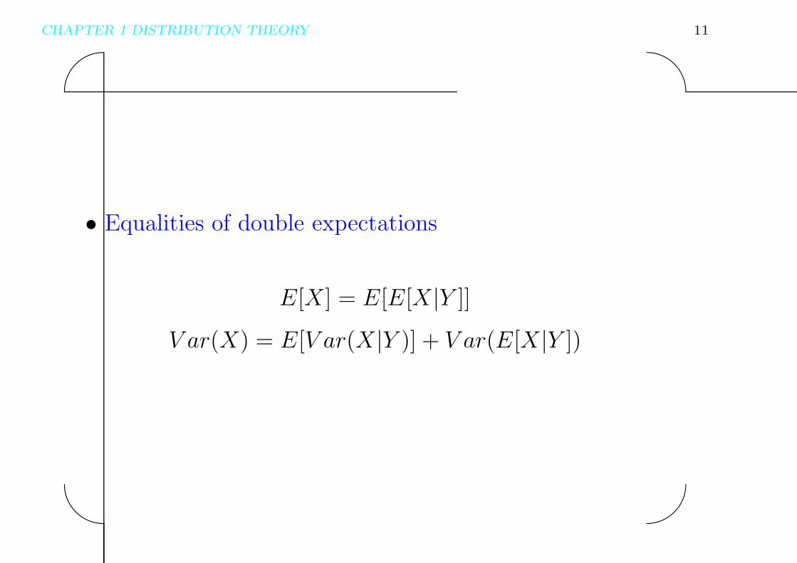
• Equalities of double expectations

E[X] = E[E[X|Y ]]

V ar(X) = E[V ar(X|Y )] + V ar(E[X|Y ])


&

$

%

[comments]


&

$

%

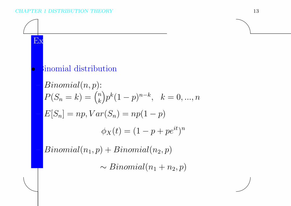
Examples of Discrete Distributions

• Binomial distribution

– Binomial(n, p):

P (Sn = k) =(nk

)pk(1− p)n−k, k = 0, ..., n

– E[Sn] = np, V ar(Sn) = np(1− p)

φX(t) = (1− p+ peit)n

– Binomial(n1, p) +Binomial(n2, p)

∼ Binomial(n1 + n2, p)


&

$

%

[comments]


&

$

%

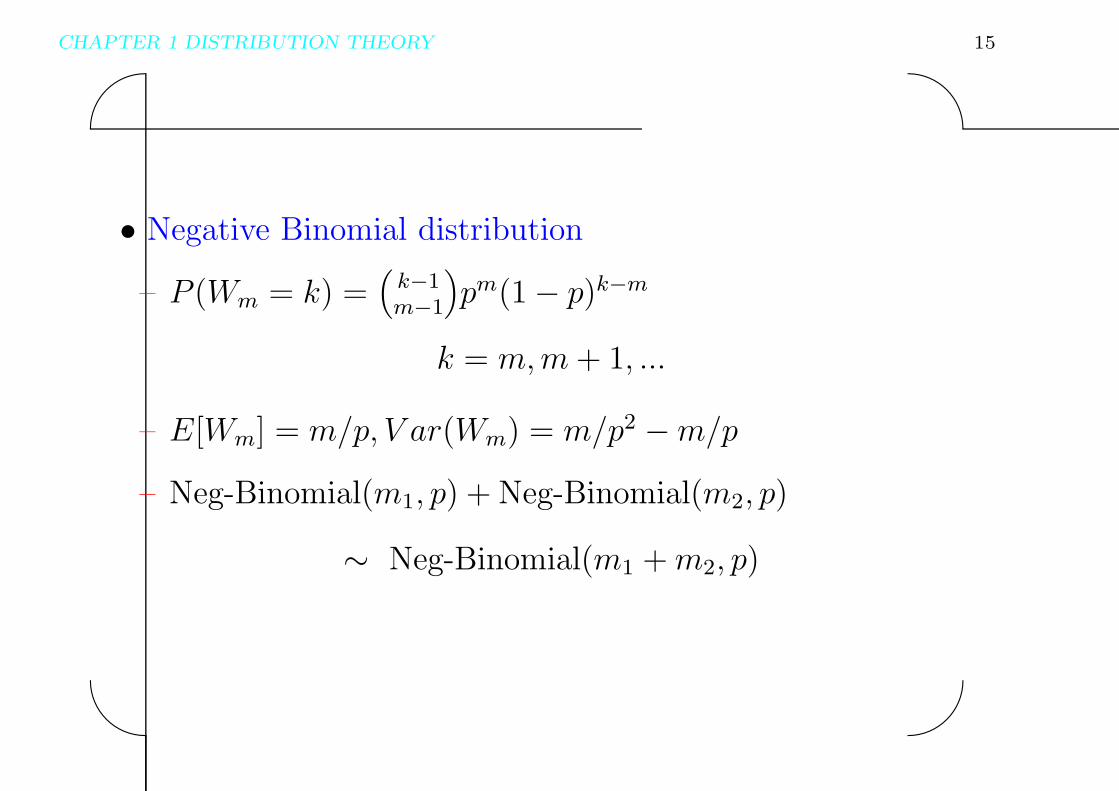
• Negative Binomial distribution

– P (Wm = k) =(k−1m−1

)pm(1− p)k−m

k = m,m+ 1, ...

– E[Wm] = m/p, V ar(Wm) = m/p2 −m/p– Neg-Binomial(m1, p) + Neg-Binomial(m2, p)

∼ Neg-Binomial(m1 +m2, p)


&

$

%

[comments]


&

$

%

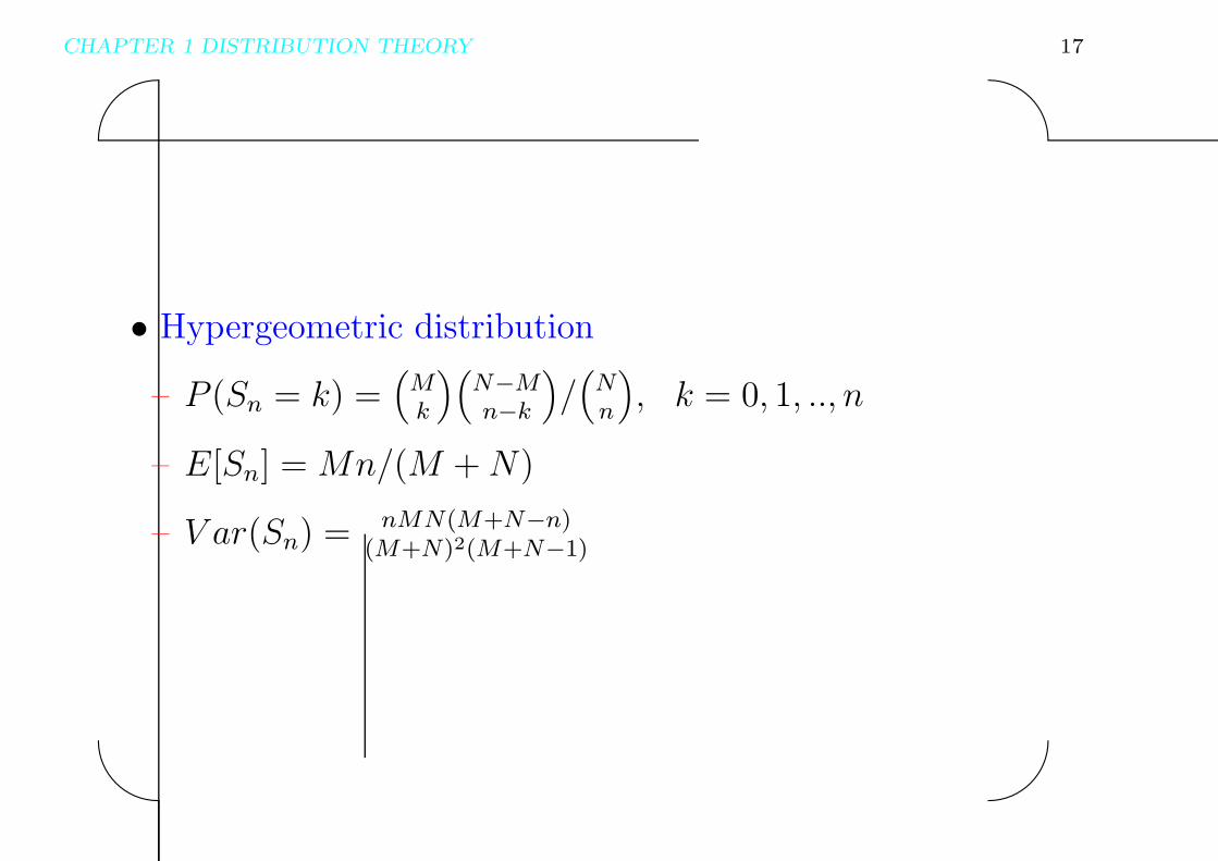
• Hypergeometric distribution

– P (Sn = k) =(Mk

)(N−Mn−k

)/(Nn

), k = 0, 1, .., n

– E[Sn] = Mn/(M + N)

– V ar(Sn) = nMN(M+N−n)(M+N)2(M+N−1)


&

$

%

[comments]


&

$

%

• Poisson distribution

– P (X = k) = λke−λ/k!, k = 0, 1, 2, ...

– E[X] = V ar(X) = λ,

φX(t) = exp{−λ(1− eit)}

– Poisson(λ1) + Poisson(λ2) ∼ Poisson(λ1 + λ2)


&

$

%

[comments]


&

$

%

• Poisson vs Binomial

– X1|X1 +X2 = n ∼ Binomial(n, λ1

λ1+λ2)

– if Xn1, ..., Xnn are i.i.d Bernoulli(pn) and npn → λ,

then

P (Sn = k) =n!

k!(n− k)!pkn(1− pn)n−k → λk

k!e−λ.


&

$

%

[comments]


&

$

%

• Multinomial Distribution

– Nl, 1 ≤ l ≤ k counts the number of times that

{Y1, ..., Yn} fall into Bl

– P (N1 = n1, ..., Nk = nk) =(

nn1,...,nk

)pn1

1 · · · pnkkn1 + ...+ nk = n

– the covariance matrix for (N1, ..., Nk)

n

p1(1− p1) . . . −p1pk...

. . ....

−p1pk . . . pk(1− pk)


&

$

%

[comments]


&

$

%

Examples of Continuous Distributions

• Uniform distribution

– Uniform(a, b): fX(x) = I[a,b](x)/(b− a)

– E[X] = (a+ b)/2 and V ar(X) = (b− a)2/12


&

$

%

[comments]


&

$

%

• Normal distribution

– N(µ, σ2): fX(x) = 1√2πσ2

exp{− (x−µ)2

2σ2 }

– E[X] = µ and V ar(X) = σ2

– φX(t) = exp{itµ− σ2t2/2}


&

$

%

[comments]


&

$

%

• Gamma distribution

– Gamma(θ, β): fX(x) = 1βθΓ(θ)

xθ−1 exp{−xβ}, x > 0

– E[X] = θβ and V ar(X) = θβ2

– θ = 1 equivalent to Exp(β)

– θ = n/2, β = 2 equivalent to χ2n


&

$

%

[comments]


&

$

%

• Cauchy distribution

– Cauchy(a, b): fX(x) = 1bπ{1+(x−a)2/b2}

– E[|X|] =∞, φX(t) = exp{iat− |bt|}– often used as counter example


&

$

%

[comments]


&

$

%

Algebra of Random Variables

• Assumption

– X and Y are independent and Y > 0

– interested in d.f. of X + Y,XY,X/Y


&

$

%

[comments]


&

$

%

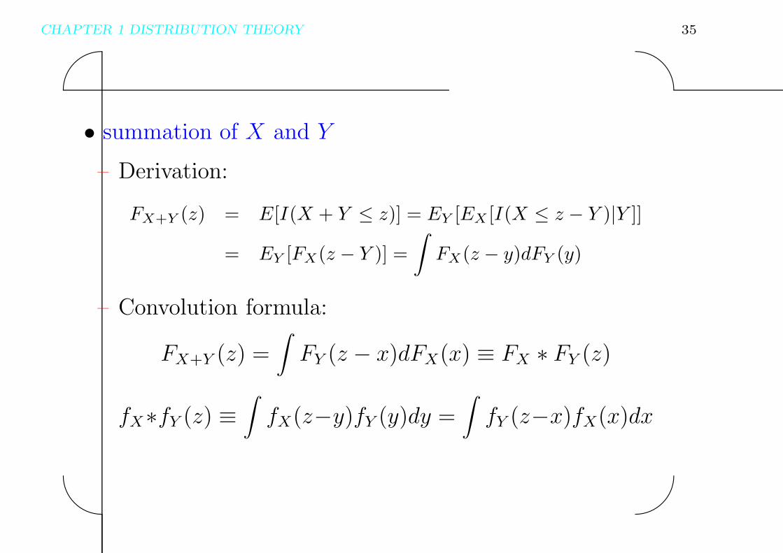
• summation of X and Y

– Derivation:

FX+Y (z) = E[I(X + Y ≤ z)] = EY [EX [I(X ≤ z − Y )|Y ]]

= EY [FX(z − Y )] =

∫FX(z − y)dFY (y)

– Convolution formula:

FX+Y (z) =∫FY (z − x)dFX(x) ≡ FX ∗ FY (z)

fX∗fY (z) ≡∫fX(z−y)fY (y)dy =

∫fY (z−x)fX(x)dx


&

$

%

[comments]


&

$

%

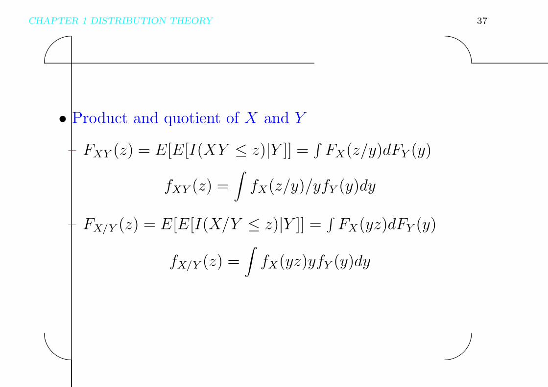
• Product and quotient of X and Y

– FXY (z) = E[E[I(XY ≤ z)|Y ]] =∫FX(z/y)dFY (y)

fXY (z) =∫fX(z/y)/yfY (y)dy

– FX/Y (z) = E[E[I(X/Y ≤ z)|Y ]] =∫FX(yz)dFY (y)

fX/Y (z) =∫fX(yz)yfY (y)dy


&

$

%

[comments]


&

$

%

• Application of formulae

– N(µ1, σ21) +N(µ2, σ

22) ∼ N(µ1 + µ2, σ

21 + σ2

2)

– Gamma(r1, θ) +Gamma(r2, θ) ∼ Gamma(r1 + r2, θ)

– Poisson(λ1) + Poisson(λ2) ∼ Poisson(λ1 + λ2)

– Negative Binomial(m1, p) + Negative Binomial(m2, p)

∼ Negative Binomial(m1 + m2, p)


&

$

%

[comments]


&

$

%

• Summation of R.V.s using c.f.

– Result: if X and Y are independent, then

φX+Y (t) = φX(t)φY (t)

– Example: X and Y are normal with

φX(t) = exp{iµ1t− σ21t

2/2},φY (t) = exp{iµ2t− σ2

2t2/2}

⇒φX+Y (t) = exp{i(µ1 + µ2)t− (σ21 + σ2

2)t2/2}


&

$

%

[comments]


&

$

%

• Further examples of special distribution

– assume X ∼ N(0, 1), Y ∼ χ2m and Z ∼ χ2

n are

independent;

–X√Y/m

∼ Student’s t(m),

Y/m

Z/n∼ Snedecor’s Fm,n,

Y

Y + Z∼ Beta(m/2, n/2).


&

$

%

[comments]


&

$

%

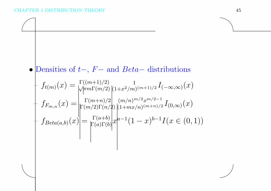
• Densities of t−, F− and Beta− distributions

– ft(m)(x) = Γ((m+1)/2)√πmΓ(m/2)

1(1+x2/m)(m+1)/2 I(−∞,∞)(x)

– fFm,n(x) = Γ(m+n)/2Γ(m/2)Γ(n/2)

(m/n)m/2xm/2−1

(1+mx/n)(m+n)/2 I(0,∞)(x)

– fBeta(a,b)(x) = Γ(a+b)Γ(a)Γ(b)

xa−1(1− x)b−1I(x ∈ (0, 1))


&

$

%

[comments]


&

$

%

• Exponential vs Beta- distributions

– assume Y1, ..., Yn+1 are i.i.d Exp(θ);

– Zi = Y1+...+YiY1+...+Yn+1

∼ Beta(i, n− i+ 1);

– (Z1, . . . , Zn) has the same joint distribution as that of

the order statistics (ξn:1, ..., ξn:n) of n Uniform(0,1)

r.v.s.


&

$

%

[comments]


&

$

%

Transformation of Random Vector

Theorem 1.3 Suppose that X is a k-dimensional

random vector with density function fX(x1, ..., xk). Let g

be a one-to-one and continuously differentiable map from

Rk to Rk. Then Y = g(X) is a random vector with

density function

fX(g−1(y1, ..., yk))|Jg−1(y1, ..., yk)|,

where g−1 is the inverse of g and Jg−1 is the Jacobian of

g−1.


&

$

%

[comments]


&

$

%

• Example

– let R2 ∼ Exp{2}, R > 0 and Θ ∼ Uniform(0, 2π) be

independent;

– X = R cos Θ and Y = R sin Θ are two independent

standard normal random variables;

– it can be applied to simulate normally distributed

data.


&

$

%

[comments]


&

$

%

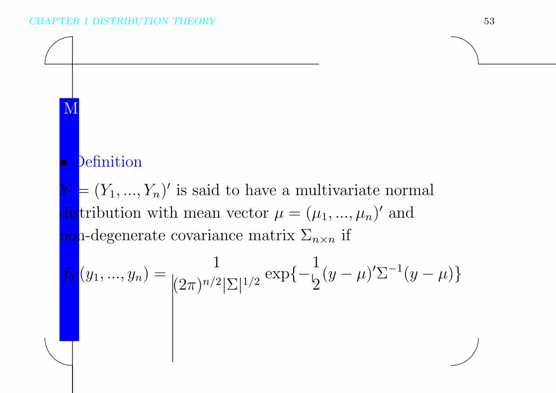
Multivariate Normal Distribution

• Definition

Y = (Y1, ..., Yn)′ is said to have a multivariate normal

distribution with mean vector µ = (µ1, ..., µn)′ and

non-degenerate covariance matrix Σn×n if

fY (y1, ..., yn) =1

(2π)n/2|Σ|1/2 exp{−1

2(y − µ)′Σ−1(y − µ)}


&

$

%

[comments]


&

$

%

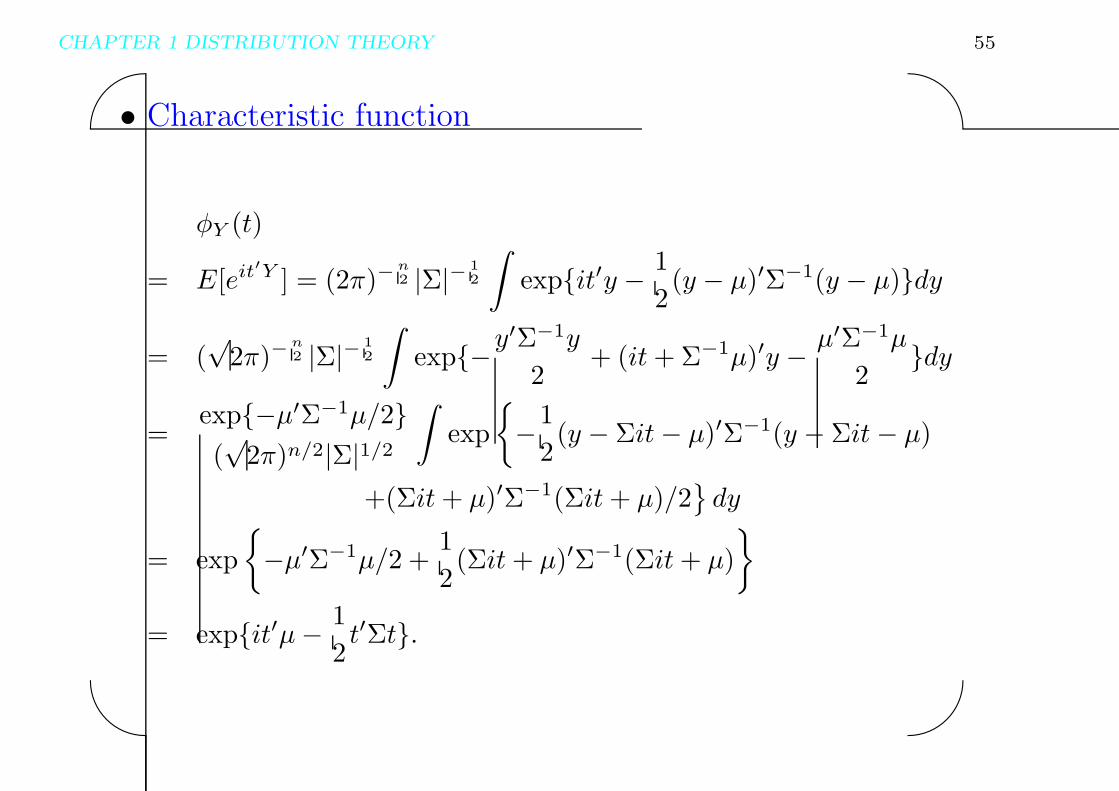
• Characteristic function

φY (t)

= E[eit′Y ] = (2π)−

n2 |Σ|− 1

2

∫exp{it′y − 1

2(y − µ)′Σ−1(y − µ)}dy

= (√

2π)−n2 |Σ|− 1

2

∫exp{−y

′Σ−1y

2+ (it+ Σ−1µ)′y − µ′Σ−1µ

2}dy

=exp{−µ′Σ−1µ/2}(√

2π)n/2|Σ|1/2∫

exp

{−1

2(y − Σit− µ)′Σ−1(y − Σit− µ)

+(Σit+ µ)′Σ−1(Σit+ µ)/2}dy

= exp

{−µ′Σ−1µ/2 +

1

2(Σit+ µ)′Σ−1(Σit+ µ)

}

= exp{it′µ− 1

2t′Σt}.


&

$

%

[comments]


&

$

%

• Conclusions

– multivariate normal distribution is uniquely

determined by µ and Σ

– for standard multivariate normal distribution,

φX(t) = exp{−t′t/2}– the moment generating function for Y is

exp{t′µ+ t′Σt/2}


&

$

%

[comments]


&

$

%

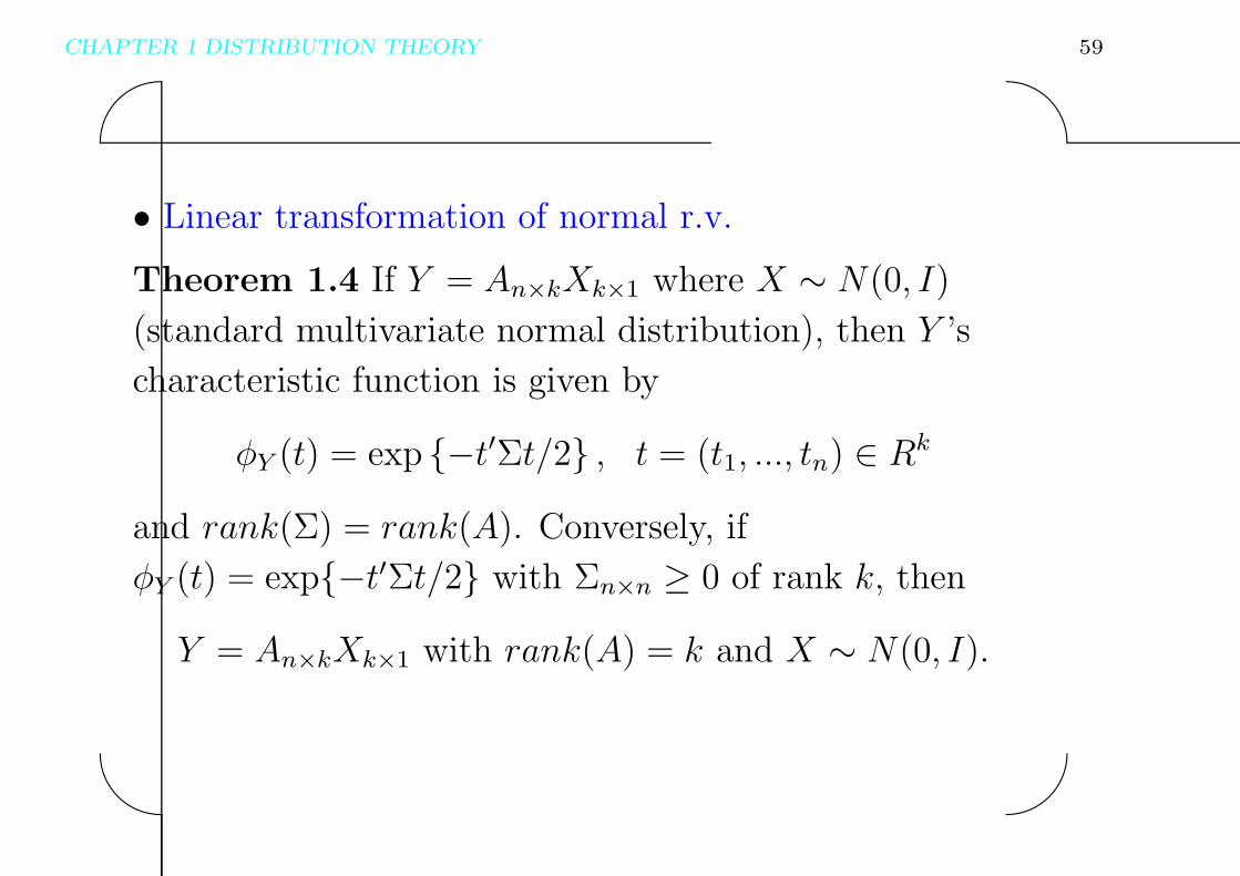
• Linear transformation of normal r.v.

Theorem 1.4 If Y = An×kXk×1 where X ∼ N(0, I)

(standard multivariate normal distribution), then Y ’s

characteristic function is given by

φY (t) = exp {−t′Σt/2} , t = (t1, ..., tn) ∈ Rk

and rank(Σ) = rank(A). Conversely, if

φY (t) = exp{−t′Σt/2} with Σn×n ≥ 0 of rank k, then

Y = An×kXk×1 with rank(A) = k and X ∼ N(0, I).


&

$

%

[comments]


&

$

%

Proof

Y = AX and X ∼ N(0, I) ⇒

φY (t) = E[exp{it′(AX)}] = E[exp{i(A′t)′X}]

= exp{−(A′t)′(A′t)/2} = exp{−t′AA′t/2}

⇒Y ∼ N(0, AA′).

Note that rank(AA′) = rank(A).


&

$

%

[comments]


&

$

%

Conversely, suppose φY (t) = exp{−t′Σt/2}. There exists O, an

orthogonal matrix, such that

Σ = O′DO, D = diag((d1, ..., dk, 0, ..., 0)′), d1, ..., dk > 0.

Define Z = OY

⇒φZ(t) = E[exp{it′(OY )}] = E[exp{i(O′t)′Y }]

= exp{− (O′t)′Σ(O′t)2

} = exp{−d1t21/2− ...− dkt2k/2}.

⇒ Z1, ..., Zk are independent N(0, d1), ..., N(0, dk) and Zk+1, ..., Zn

are zeros.

⇒ Let Xi = Zi/√di, i = 1, ..., k and O′ = (Bn×k, Cn×(n−k)).

Y = O′Z = Bdiag{(√d1, ...,

√dk)}X ≡ AX.

Clearly, rank(A) = k.


&

$

%

[comments]


&

$

%

• Conditional normal distributions

Theorem 1.5 Suppose that Y = (Y1, ..., Yk, Yk+1, ..., Yn)′

has a multivariate normal distribution with mean

µ = (µ(1)′, µ(2)′)′ and a non-degenerate covariance matrix

Σ =

(Σ11 Σ12

Σ21 Σ22

).

Then

(i) (Y1, ..., Yk)′ ∼ Nk(µ

(1),Σ11).

(ii) (Y1, ..., Yk)′ and (Yk+1, ..., Yn)′ are independent if and

only if Σ12 = Σ21 = 0.

(iii) For any matrix Am×n, AY has a multivariate normal

distribution with mean Aµ and covariance AΣA′.


&

$

%

[comments]


&

$

%

(iv) The conditional distribution of Y (1) = (Y1, ..., Yk)′

given Y (2) = (Yk+1, ..., Yn)′ is a multivariate normal

distribution given as

Y (1)|Y (2) ∼ Nk(µ(1)+Σ12Σ−1

22 (Y (2)−µ(2)),Σ11−Σ12Σ−122 Σ21).


&

$

%

[comments]


&

$

%

Proof

Prove (iii) first. φY (t) = exp{it′µ− t′Σt/2}.

⇒ φAY (t) = E[eit′AY ] = E[ei(A

′t)′Y ]

= exp{i(A′t)′µ− (A′t)′Σ(A′t)/2}

= exp{it′(Aµ)− t′(AΣA′)t/2}

⇒ AY ∼ N(Aµ,AΣA′).


&

$

%

[comments]


&

$

%

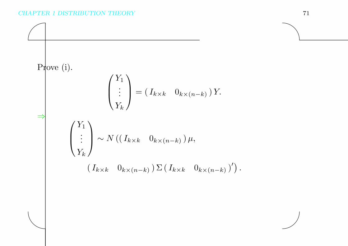
Prove (i). Y1...

Yk

= ( Ik×k 0k×(n−k) )Y.

⇒ Y1...

Yk

∼ N (( Ik×k 0k×(n−k) )µ,

( Ik×k 0k×(n−k) ) Σ ( Ik×k 0k×(n−k) )′).


&

$

%

[comments]


&

$

%

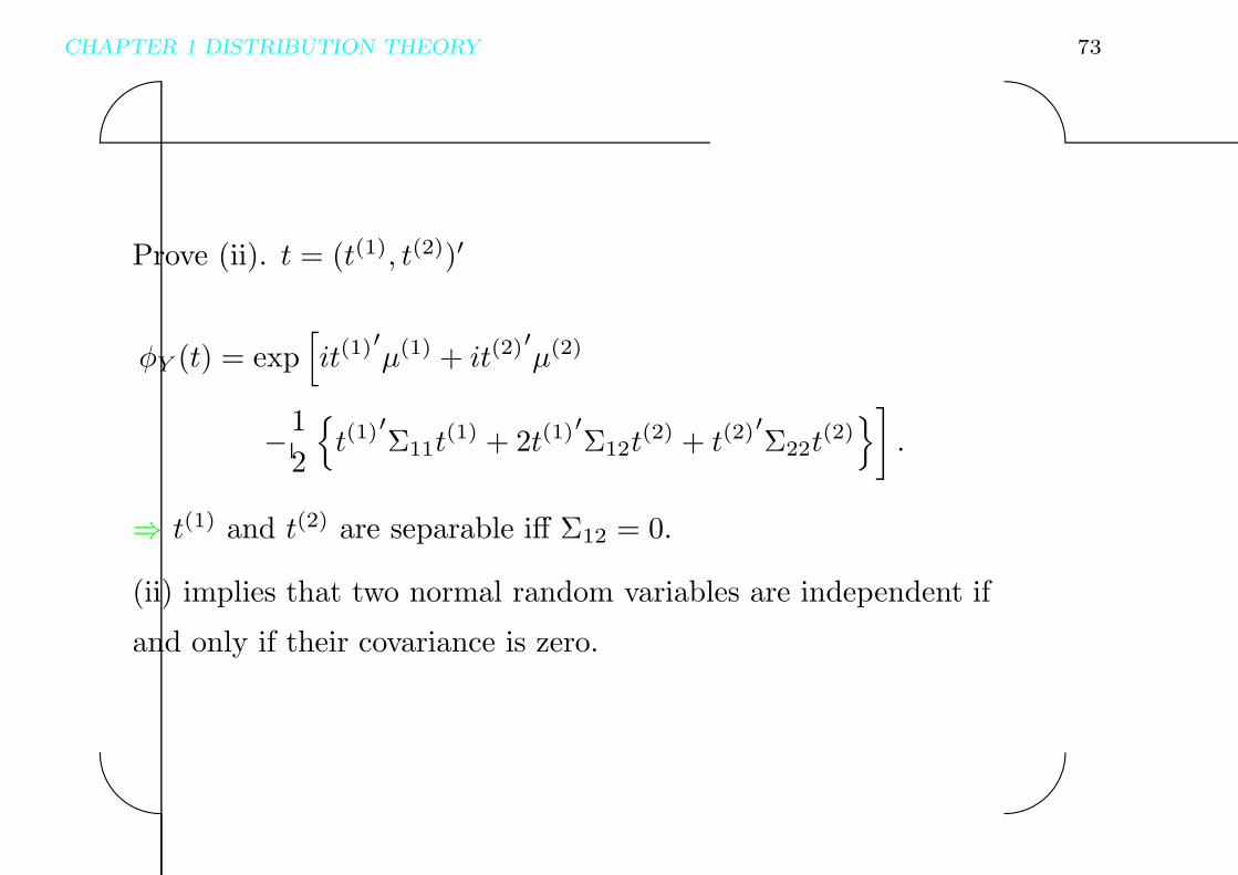
Prove (ii). t = (t(1), t(2))′

φY (t) = exp[it(1)′µ(1) + it(2)′µ(2)

−1

2

{t(1)′Σ11t

(1) + 2t(1)′Σ12t(2) + t(2)′Σ22t

(2)}]

.

⇒ t(1) and t(2) are separable iff Σ12 = 0.

(ii) implies that two normal random variables are independent if

and only if their covariance is zero.


&

$

%

[comments]


&

$

%

Prove (iv). Consider

Z(1) = Y (1) − µ(1) − Σ12Σ−122 (Y (2) − µ(2)).

⇒ Z(1) ∼ N(0,ΣZ)

ΣZ = Cov(Y (1), Y (1))− 2Σ12Σ−122 Cov(Y (2), Y (1))

+Σ12Σ−122 Cov(Y (2), Y (2))Σ−1

22 Σ21 = Σ11 − Σ12Σ−122 Σ21.

Cov(Z(1), Y (2)) = Cov(Y (1), Y (2))− Σ12Σ−122 Cov(Y (2), Y (2)) = 0.

⇒ Z(1) is independent of Y (2).

⇒ The conditional distribution of Z(1) given Y (2) is the same as

the unconditional distribution of Z(1)

⇒ Z(1)|Y (2) ∼ Z(1) ∼ N(0,Σ11 − Σ12Σ−122 Σ21).


&

$

%

[comments]


&

$

%

• Remark on Theorem 1.5

– The constructed Z in (iv) has a geometric

interpretation using the projection of (Y (1) − µ(1)) on

the normalized variable Σ−1/222 (Y (2) − µ(2)).


&

$

%

[comments]


&

$

%

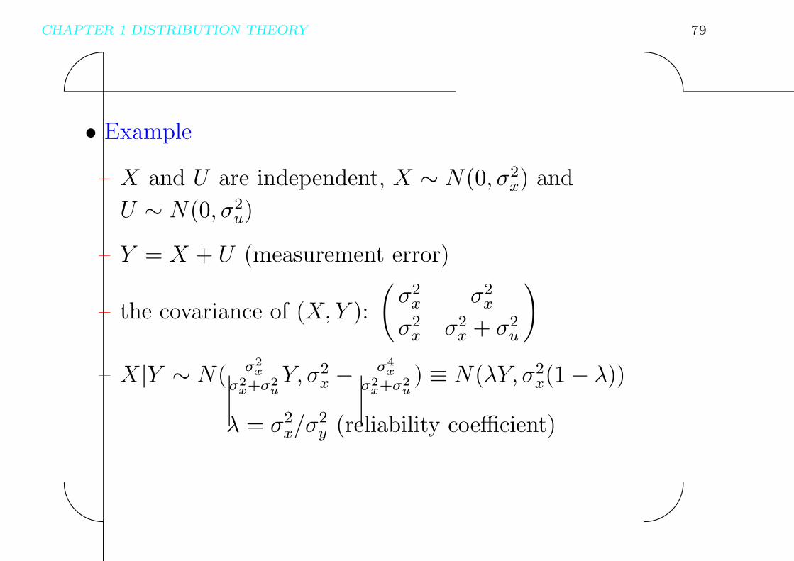
• Example

– X and U are independent, X ∼ N(0, σ2x) and

U ∼ N(0, σ2u)

– Y = X + U (measurement error)

– the covariance of (X,Y ):

(σ2x σ2

x

σ2x σ2

x + σ2u

)

– X|Y ∼ N( σ2x

σ2x+σ2

uY, σ2

x − σ4x

σ2x+σ2

u) ≡ N(λY, σ2

x(1− λ))

λ = σ2x/σ

2y (reliability coefficient)


&

$

%

[comments]


&

$

%

• Quadratic form of normal random variables

– N(0, 1)2 + ...+ N(0, 1)2 ∼ χ2n ≡ Gamma(n/2, 2).

– If Y ∼ Nn(0,Σ) with Σ > 0, then Y ′Σ−1Y ∼ χ2n.

– Proof:

Y = AX where X ∼ N(0, I) and Σ = AA′.

Y ′Σ−1Y = X ′A′(AA′)−1AX = X ′X ∼ χ2n.


&

$

%

[comments]


&

$

%

• Noncentral Chi-square distribution

– assume X ∼ N(µ, I)

– Y = X ′X ∼ χ2n(δ) and δ = µ′µ.

– Y ’s density:

fY (y) =∞∑

k=0

exp{−δ/2}(δ/2)k

k!g(y; (2k + n)/2, 1/2).


&

$

%

[comments]


&

$

%

• Additional notes on normal distributions

– noncentral t-distribution: N(δ, 1)/√χ2n/n

noncentral F -distribution: χ2n(δ)/n/(χ2

m/m)

– how to calculate E[X ′AX] where X ∼ N(µ,Σ):

E[X ′AX] = E[tr(X ′AX)] = E[tr(AXX ′)]

= tr(AE[XX ′]) = tr(A(µµ′ + Σ))

= µ′Aµ+ tr(AΣ)


&

$

%

[comments]


&

$

%

Families of Distributions

• location-scale family

– aX + b: fX((x− b)/a)/a, a > 0, b ∈ R– mean aE[X] + b and variance a2V ar(X)

– examples: normal distribution, uniform distribution,

gamma distributions, etc.


&

$

%

[comments]


&

$

%

• Exponential family

– examples: binomial, Poisson distributions for discrete

variables and normal distribution, gamma

distribution, Beta distribution for continuous

variables

– has a general expression of densities

– possesses nice statistical properties


&

$

%

[comments]


&

$

%

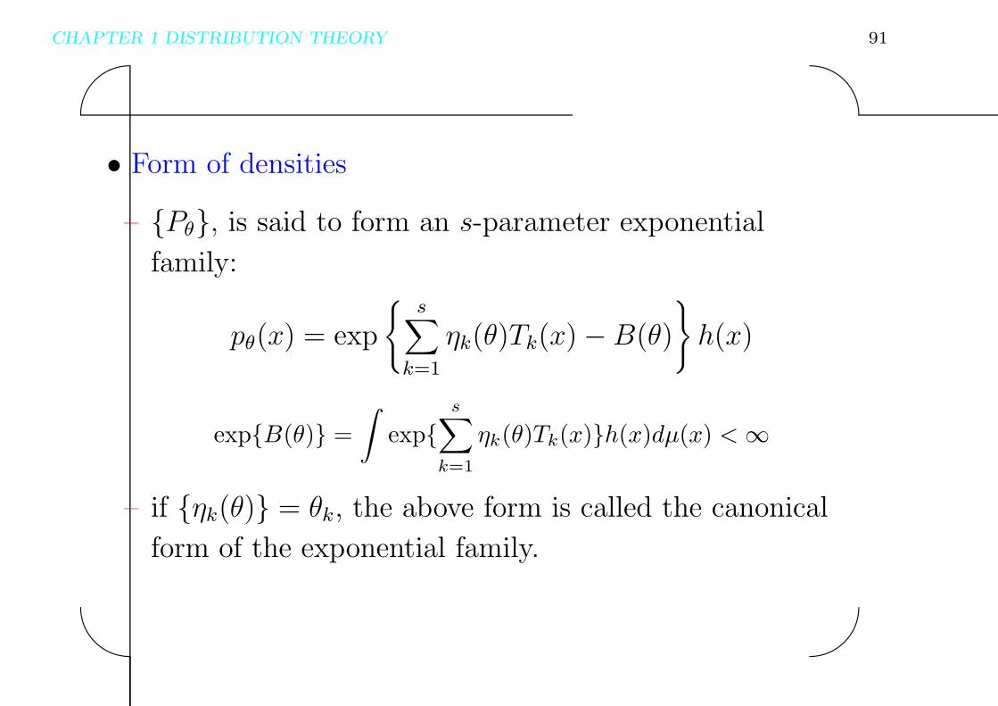
• Form of densities

– {Pθ}, is said to form an s-parameter exponential

family:

pθ(x) = exp

{s∑

k=1

ηk(θ)Tk(x)−B(θ)

}h(x)

exp{B(θ)} =

∫exp{

s∑

k=1

ηk(θ)Tk(x)}h(x)dµ(x) <∞

– if {ηk(θ)} = θk, the above form is called the canonical

form of the exponential family.


&

$

%

[comments]


&

$

%

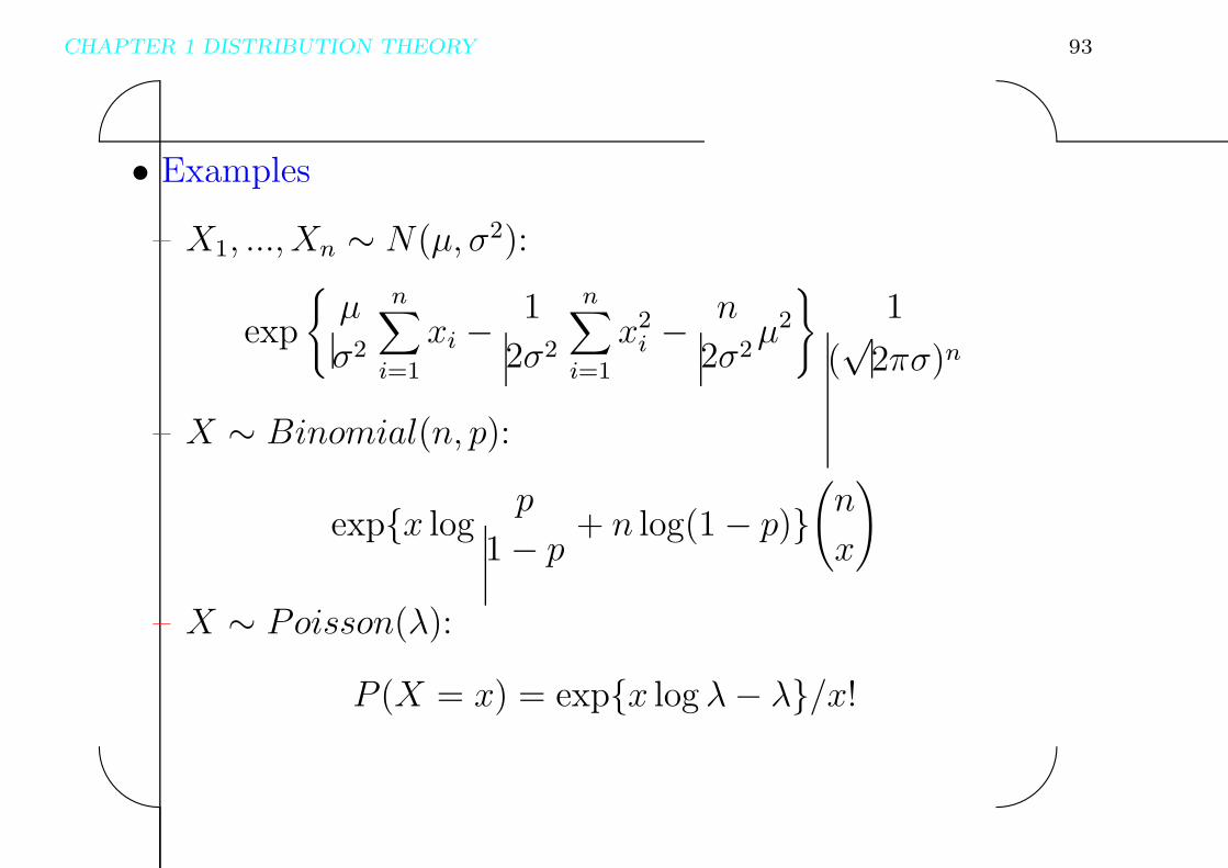
• Examples

– X1, ..., Xn ∼ N(µ, σ2):

exp

{µ

σ2

n∑

i=1

xi −1

2σ2

n∑

i=1

x2i −

n

2σ2µ2

}1

(√

2πσ)n

– X ∼ Binomial(n, p):

exp{x logp

1− p + n log(1− p)}(n

x

)

– X ∼ Poisson(λ):

P (X = x) = exp{x log λ− λ}/x!


&

$

%

[comments]


&

$

%

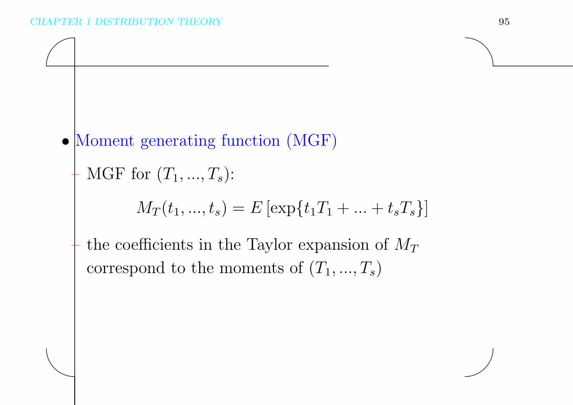
• Moment generating function (MGF)

– MGF for (T1, ..., Ts):

MT (t1, ..., ts) = E [exp{t1T1 + ...+ tsTs}]

– the coefficients in the Taylor expansion of MT

correspond to the moments of (T1, ..., Ts)


&

$

%

[comments]


&

$

%

• Calculate MGF in the exponential family

Theorem 1.6 Suppose the densities of an exponential

family can be written as the canonical form

exp{s∑

k=1

ηkTk(x)− A(η)}h(x),

where η = (η1, ..., ηs)′. Then for t = (t1, ..., ts)

′,

MT (t) = exp{A(η + t)− A(η)}.


&

$

%

[comments]


&

$

%

Proof

exp{A(η)} =∫

exp{∑sk=1 ηiTi(x)}h(x)dµ(x).

⇒MT (t) = E [exp{t1T1 + ...+ tsTs}]

=

∫exp{

s∑

k=1

(ηi + ti)Ti(x)−A(η)}h(x)dµ(x)

= exp{A(η + t)−A(η)}.


&

$

%

[comments]


&

$

%

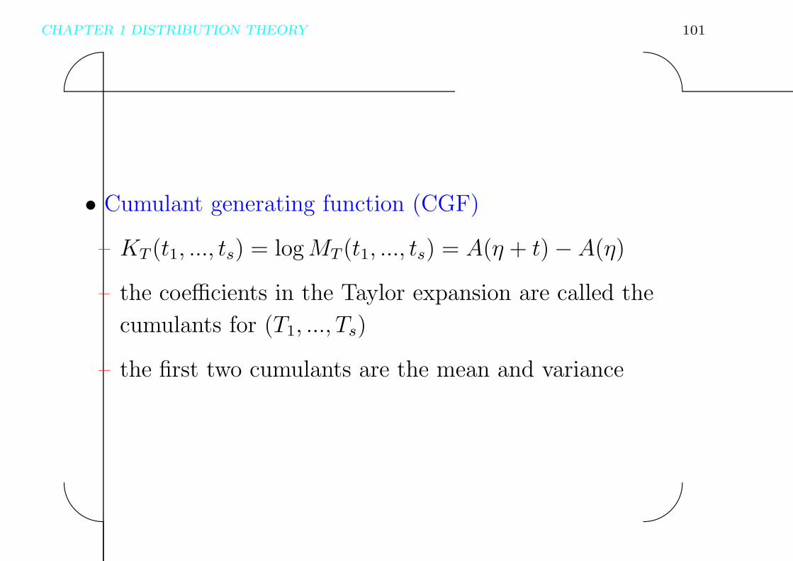
• Cumulant generating function (CGF)

– KT (t1, ..., ts) = logMT (t1, ..., ts) = A(η + t)− A(η)

– the coefficients in the Taylor expansion are called the

cumulants for (T1, ..., Ts)

– the first two cumulants are the mean and variance


&

$

%

[comments]


&

$

%

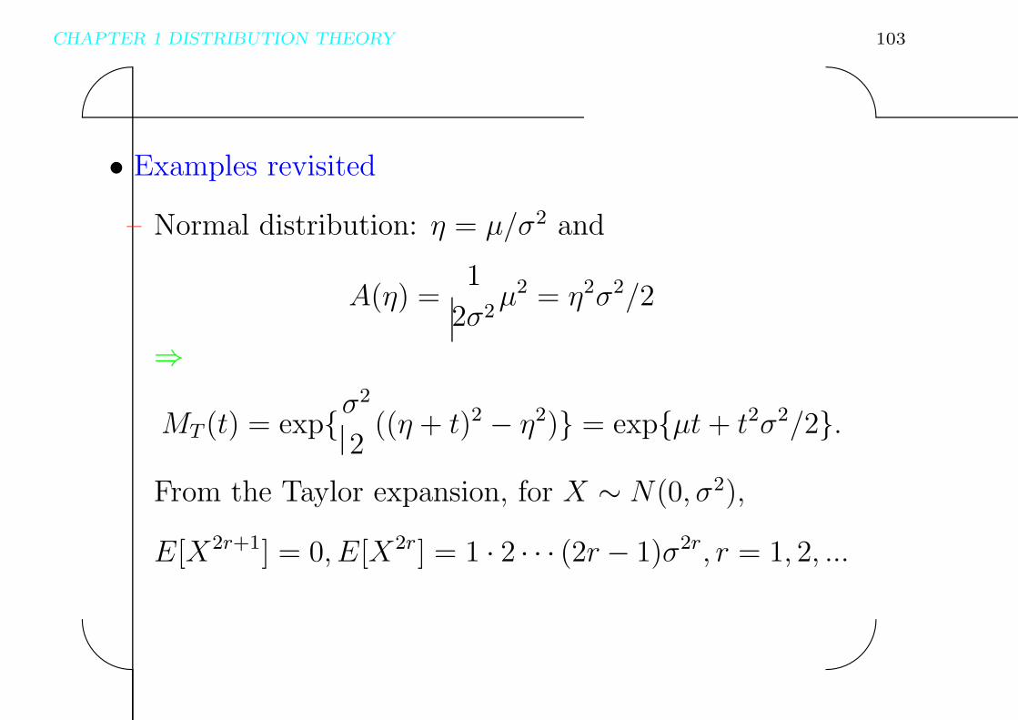
• Examples revisited

– Normal distribution: η = µ/σ2 and

A(η) =1

2σ2µ2 = η2σ2/2

⇒

MT (t) = exp{σ2

2((η + t)2 − η2)} = exp{µt+ t2σ2/2}.

From the Taylor expansion, for X ∼ N(0, σ2),

E[X2r+1] = 0, E[X2r] = 1 · 2 · · · (2r − 1)σ2r, r = 1, 2, ...


&

$

%

[comments]


&

$

%

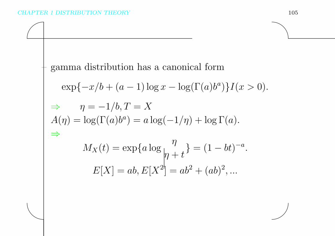
– gamma distribution has a canonical form

exp{−x/b + (a− 1) log x− log(Γ(a)ba)}I(x > 0).

⇒ η = −1/b, T = X

A(η) = log(Γ(a)ba) = a log(−1/η) + log Γ(a).

⇒MX(t) = exp{a log

η

η + t} = (1− bt)−a.

E[X] = ab, E[X2] = ab2 + (ab)2, ...


&

$

%

[comments]


&

$

%

READING MATERIALS : Lehmann and Casella,

Sections 1.4 and 1.5

Documents

Basic Concepts Random Variables { discrete random …kosorok/bios760sub/ChapA_Slide+Note.pdf · { discrete random variable: probability mass function { continuous random variable: